Combining homogeneous and heterogeneous chemistry to model inorganic compound concentrations in indoor environments: the H²I model (v1.0)

Homogeneous reactivity has been extensively studied in recent years through outdoor air-quality simulations. However, indoor atmospheres are known to be largely influenced by another type of chemistry, which is their reactivity with surfaces. Despite progress in the understanding of heterogeneous reactions, such reactions remain barely integrated into numerical models. In this paper, a room-scale, indoor air-quality (IAQ) model is developed to represent both heterogeneous and homogeneous chemistry. Thanks to the introduction of sorbed species, deposition and surface reactivity are treated as two separate processes, and desorption reactions are incorporated. The simulated concentrations of inorganic species are compared with experimental measurements acquired in a real room, thus allowing calibration of the model's undetermined parameters. For the duration of the experiments, the influence of the simulation's initial conditions is strong. The model succeeds in simulating the four inorganic species concentrations that were measured, namely NO, NO₂, HONO and O₃. Each parameter is then varied to estimate its sensitivity and to identify the most prevailing processes. The air-mixing velocity and the building filtration factor are uncertain parameters that appear to have a strong influence on deposition and on the control of transport from outdoors, respectively. As expected, NO₂ surface hydrolysis plays a key role in the production of secondary species. The secondary production of NO by the reaction of sorbed HONO with sorbed HNO₃ stands as an essential component to integrate into IAQ models.

1 Introduction

At a time when sustainable development requires more effort than ever, the improvement of building isolation has become a major concern in the field of construction and renovation. Apart from being necessary for the health and comfort of the occupants, airtight conceptions are needed to curb the energy consumption of accommodations and offices and thus decrease their carbon footprint. However, as air remains more confined with a lower exchange rate with the outdoors, the pollutants generated indoors have fewer possibilities to escape, which raises health issues. It is now established that indoor atmospheres are more polluted than those outdoors, while we spend most of our time in indoor environments: up to 90 % in developed countries (Carslaw, 2007). In this context, indoor air quality (IAQ) is bound to be an increasingly important issue.

Whereas numerical simulations appear to be a standard approach for the study of outdoor atmospheres, they are less common in the field of indoor environments. Indoor environments are complex, and processes relying on the surface-to-volume ratio, which are still not fully understood but often negligible outdoors, are predominantly important in indoor environments (Weschler, 2011).

Historically, early attempts to model indoor atmospheres focused on the correct assessment of primary emissions, considering each chemical component independently. The model of Nazaroff and Cass (1986) provided the first description of the indoor environment as a chemically reactive homogeneous system, taking into account the interactions of about 30 species and groups of species based on a modified version of the Falls and Seinfeld (1978) mechanism. They included photolytic reactions and a simple form of deposition, considering decomposition and irreversible absorption reactions. Sarwar et al. (2002) adapted the chemical mechanism SAPRC-99 in order to take into account newer advances in O₃ reactions with alkene. In particular, they introduced the chemistry of 40 volatile organic compounds (VOCs) recognized as atmospheric pollutants. Deposition was modelled as in Nazaroff and Cass (1986), and no deposition was assumed for species for which no deposition velocity was available. A more detailed chemical mechanism was tested by Carslaw (2007), who adapted the Master Chemical Mechanism (MCM) to indoor environments, including about 4600 species and 15 400 reactions. Deposition was modelled similarly to Nazaroff and Cass (1986), and for the first time, a heterogeneous reaction on indoor surfaces was considered by introducing a production rate accounting for HONO secondary formation. Later, Mendez et al. (2015) implemented a simplified version of the SAPRC-07 mechanism and described deposition as a two-step process by making a distinction between transport from free space to a surface and reactivity with the surface. Further details were provided by Mendez et al. (2017), who parameterized the mass transfer effect using a model of transport-limited deposition velocity.

As highlighted by Weschler (2011), surface chemistry is responsible for secondary pollutant formation that can be of greater importance for IAQ than primary emissions. Because heterogeneous reactions can be faster than their equivalent gas-phase homogeneous reaction, their importance relative to the air exchange rate and thus their influence on indoor atmospheres are large. Secondary pollutants can persist a long time after the reagent species have been reduced to negligible levels and are very difficult to anticipate due to their strong dependence on ambient conditions.

The heterogeneous hydrolysis of NO₂ is one of these reactions and is recognized as the main source of HONO in indoor environments. There is evidence that certain surfaces can act as a reservoir of sorbed NO₂ and that these surfaces can release HONO long after the decay of NO₂ (Wainman et al., 2001). Presumably, this HONO surface release depends on the ambient NO₂ concentration, ambient relative humidity and the surface ability to retain water.

As a rule, it is assumed that the heterogeneous hydrolysis of NO₂ leads to the formation of HONO and HNO₃ following the stoichiometry proposed by Febo and Perrino (1991):

$$\begin{array}{}\text{(R1)}& \mathrm{2}{\mathrm{NO}}_{\mathrm{2}}+{\mathrm{H}}_{\mathrm{2}}\mathrm{O}\to \mathrm{HONO}+{\mathrm{HNO}}_{\mathrm{3}}.\end{array}$$

Contrary to HONO, HNO₃ is not observed as a gas-phase product in this process due to its strong adsorption capacity. HNO₃ remains on the surface and can react with other species. Namely, Mochida and Finlayson-Pitts (2000) studied the production of NO₂ by the reaction of HNO₃ with gaseous NO on porous glass. They showed that the NO concentration cannot decay below a threshold value, suggesting NO regeneration pathways. Coherently, NO formation was pointed out during NO₂ hydrolysis experiments, simultaneously to NO₂ exposure or at longer reaction times. Finlayson-Pitts et al. (2003) measured for this reaction a HONO yield that was much less than 50 % of the NO₂ loss and observed that the yield of NO relative to HONO increased with time. Based on their own and previously reported observations, they suggested NO could be formed by the secondary auto-ionization of the sorbed HONO as

$$\begin{array}{}\text{(R2)}& \mathrm{2}\mathrm{HONO}\to \mathrm{NO}+{\mathrm{NO}}_{\mathrm{2}}+{\mathrm{H}}_{\mathrm{2}}\mathrm{O}\end{array}$$

and also by conversion of the sorbed HONO following a mechanism that involves HNO₃ and simplifies to the net reaction

$$\begin{array}{}\text{(R3)}& \mathrm{HONO}+{\mathrm{HNO}}_{\mathrm{3}}\to \mathrm{2}\mathrm{NO}+{\mathrm{H}}_{\mathrm{2}}\mathrm{O}+{\mathrm{O}}_{\mathrm{2}}.\end{array}$$

Considering longer reaction times, NO could also react with HNO₃ following the reaction (Finlayson-Pitts et al., 2003)

$$\begin{array}{}\text{(R4)}& \mathrm{NO}+{\mathrm{HNO}}_{\mathrm{3}}\to \mathrm{HONO}+{\mathrm{NO}}_{\mathrm{2}}.\end{array}$$

Finally, the photochemical enhancement of HONO production during NO₂ hydrolysis was investigated by Ramazan et al. (2004), who showed that NO₂ hydrolysis was not photo-enhanced but that HONO production was fostered by another process, which was likely the photolysis of sorbed HNO₃ caused by UV rays. Other heterogeneous reactions could be pointed out, especially those involving O₃, which is known to have a significant adsorption capacity.

Reviewing the state of the art of surface reactions unveils a serious void in the modelling of indoor atmospheres. Current models incorporate these phenomena very incompletely due to the strong uncertainties they are subjected to. In particular, the ratio of the production of NO compared with HONO during NO₂ hydrolysis derives from mechanisms that are still unclear. The detailed scheme proposed by Finlayson-Pitts et al. (2003) involves reactions of several intermediate species whose reaction rates are unknown. As a test, they introduced this scheme in the kinetic programme REACT to compute the loss of NO₂ and formation of HONO and NO, and they adjusted the required rate constants to obtain a good match with their cell experimental data. In this model, uptake and reactions on surfaces were not explicitly treated, which caused heterogeneous reactions to be implemented as gas-phase reactions. Ramazan et al. (2004) conducted similar work, and the parameterization they proposed was later used by Courtey et al. (2009) to model confined atmospheres, i.e. without including ventilation and primary emissions.

In this work, a room-scale IAQ model is developed to incorporate the heterogeneous chemistry described above, in addition to the homogeneous chemistry already considered by box models. The concentrations simulated by this model are compared with measurements that were performed in a real office (Gandolfo, 2018; Gandolfo et al., 2021) from 27 to 31 October 2016 in Martigues (France). The aim of these measurements was to study the impact of photocatalytic paints characterized in laboratory experiments (Gandolfo et al., 2015, 2017) on indoor atmosphere health. Whereas laboratory tests had been conducted with paints containing up to 7 % TiO₂ nanoparticles, this campaign was restricted to a non-photocatalytic paint (reference paint) and to the same paint enriched with a commercially viable amount of 3.5 % TiO₂ nanoparticles. Two types of measurements were obtained using either UV-blocking or borosilicate windows. The simulations presented in this paper are compared with the data obtained with the UV-blocking window only to minimize the effect of photo-induced processes, which will be studied in a separate paper. The organic compound concentrations are fixed to their measured values to focus on the modelling of inorganic species.

The present model, called the H²I (homogeneous heterogeneous indoor) model, assumes a uniformly mixed environment, taking into account emissions, ventilation, chemistry and deposition processes. The chemical mechanism solving the gas-phase chemistry is a version of the RACM2 chemical scheme (Goliff et al., 2013) based upon the earlier Regional Atmospheric Chemistry Mechanism (RACM; Stockwell et al., 1997) implemented in the Polyphemus air-quality modelling platform (Kim et al., 2009). Deposition is modelled as in Mendez et al. (2017). As in Finlayson-Pitts et al. (2003) and Ramazan et al. (2004), the rate constants of the heterogeneous reactions are adjusted to obtain a reasonable match to the experimental data. Contrary to other box models (Nazaroff and Cass, 1986; Sarwar et al., 2002; Carslaw, 2007; Courtey et al., 2009; Mendez et al., 2015), this model does not assume that the light is homogeneous throughout the room. Here, two different parts are considered: one irradiated by direct light and another illuminated indirectly. This is one of the first models to consider the evolution of light intensity in each part through the day, as well as the volumes that they occupy, without making use of computational fluid dynamics (CFD) simulations (Won et al., 2019).

First, this paper provides a detailed description of the H²I model. The input data and the tuneable parameters of the model are then described. These parameters are calibrated by comparing the simulation results to the concentration profiles that were acquired in Martigues (France). For each experiment, the set of parameters leading to the best simulation, called the reference simulation, is provided. Each of the parameters is then varied to estimate its sensitivity, thereby identifying the most impacting processes. Finally, a surface saturation limit is implemented to test the model in high NO₂ conditions.

2 Presentation of the H²I (homogeneous heterogeneous indoor) model

2.1 Mass balance equation

The room is divided into two volumes: a volume illuminated by the light of the sun and a darker volume illuminated by indirect light. As the light in these two volumes has different intensities, the magnitudes of the photolytic reactions occurring inside these volumes are different, leading to different concentrations in each volume (see Fig. 1 for a schema). $m_i^j$ [μg] is the mass of species i in the box j, with j = {L,G}, L denoting the sunlit box illuminated by direct light, and G denoting the gloomy box illuminated indirectly by diffuse and reflected light (see Appendix A for a summary of the symbols used). The evolution of $m_i^j$ with time is given by the classical box model equation (e.g. Sarwar et al., 2002; Carslaw, 2007) complemented by a box exchange term (Furtaw et al., 1996):

$$\begin{array}{}\text{(1)}& \begin{array}{rl}{\displaystyle \frac{\text{d}{m}_i^j}{\text{d}t}}=& k_{\mathrm{AER}}f{m}_i^{\mathrm{Out},j}-k_{\mathrm{AER}}{m}_i^j-k_{\mathrm{DEP},i}^j{m}_i^j\\ & +k_{\mathrm{BOX}}^j{\mathrm{\Delta }}_j{m}_i+\sum _p{Q}_{pi}^j+\sum _q{R}_{iq}^j,\end{array}\end{array}$$

where t is the time [s], k_AER is the air exchange rate between the room and outside the room [s⁻¹], including the rest of the building, f is the outdoor-to-indoor filtration factor [–] (i.e. the fraction of air exchange with outdoors), $m_i^{\mathrm{Out},j}$ is the outdoor mass of species i introduced in box j [µg], $k_{\mathrm{DEP},i}^j$ is the deposition rate of species i [s⁻¹], k_BOX is the air exchange rate between the boxes [s⁻¹], Δ_jm_i is the corresponding mass transfer [µg], Q_pi is the emission rate of source p [µg s⁻¹], and $R_{iq}^j$ is the mass reaction rate between species i and species q [µg s⁻¹].

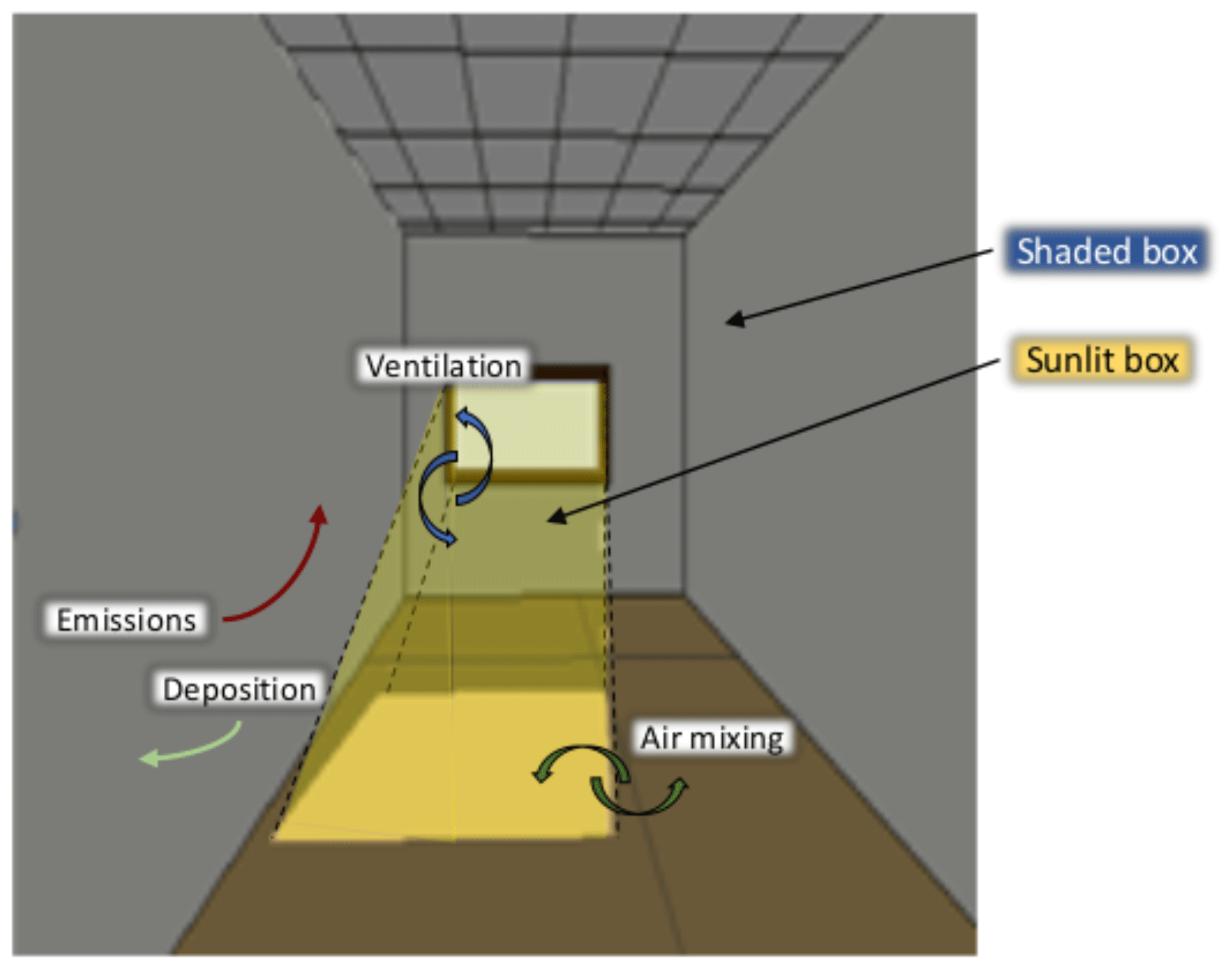
Figure 1 Schema of the sunlit and shaded boxes in the experiment room at 13:00 on 30 October.

By denoting $V_{\mathrm{box}}^j$ as the volume of the box j [m³], the mass transfer from box L to box S is expressed as

$$\begin{array}{}\text{(2)}& {\mathrm{\Delta }}_L{m}_i=-m_i^L+{\displaystyle \frac{V_{\mathrm{box}}^L}{V_{\mathrm{box}}^G}}{m}_i^G,\end{array}$$

and the mass transfer from box S to box L is expressed as

$$\begin{array}{}\text{(3)}& {\mathrm{\Delta }}_G{m}_i={\displaystyle \frac{V_{\mathrm{box}}^G}{V_{\mathrm{box}}^L}}{m}_i^L-m_i^G.\end{array}$$

The evolution of the species concentrations is obtained by dividing Eq. (1) by the box volume. This yields

$$\begin{array}{}\text{(4)}& \begin{array}{rl}{\displaystyle \frac{\text{d}{C}_i^j}{\text{d}t}}=& k_{\mathrm{AER}}f{C}_i^{\mathrm{Out}}-k_{\mathrm{AER}}{C}_i^j-k_{\mathrm{DEP},i}^j{C}_i^j+k_{\mathrm{BOX}}^j{\mathrm{\Delta }}_j{C}_i\\ & +\sum _p{\displaystyle \frac{Q_{pi}^j}{V_{\mathrm{box}}^j}}+\sum _q{\displaystyle \frac{R_{iq}^j}{V_{\mathrm{box}}^j}},\end{array}\end{array}$$

where $C_i^j=m_i^j/V_{\mathrm{box}}^j$ is the indoor concentration of species i in volume j [µg m⁻³], $C_i^{\mathrm{Out}}$ is the outdoor concentration of species i [µg m⁻³] and Δ_jC_i is the concentration variation caused by the gas transfers between boxes [µg m⁻³], given by

$$\begin{array}{}\text{(5)}& \begin{array}{rl}{\mathrm{\Delta }}_L{C}_i& =-C_i^L+C_i^G,\\ {\mathrm{\Delta }}_G{C}_i& =C_i^L-C_i^G.\end{array}\end{array}$$

On the right-hand side of Eq. (4), the first term is the intake of species coming from outdoors. The second term is the concentration loss due to the leakages not only to the outdoors but also to the other rooms in the building. The third term is deposition. The fourth term represents the mixing between the two volumes. The fifth term represents the indoor sources that release species i, and the last term is the contribution of the reactions involving species i.

The two types of sources encountered in the experiments of this campaign are the emissions of the paint boards placed on the walls (Q_paint,i) and the emissions from the building (Q_room,i) released by the building materials, furniture and appliances of the neighbouring rooms. The room emissions in the box j can be written as

$$\begin{array}{}\text{(6)}& Q_{\mathrm{room},i}^j=Q_{\mathrm{room},i}{\displaystyle \frac{V_{\mathrm{box}}^j}{V_{\mathrm{room}}}},\end{array}$$

where V_room=32.8 m³ is the total volume of the room. The paint emissions are derived from their surface emission rates:

$$\begin{array}{}\text{(7)}& Q_{\mathrm{paint},i}^j=E_{\mathrm{paint},i}^j{S}_{\mathrm{paint}}^j,\end{array}$$

where E_paint,i represents the paint surface emission rates obtained experimentally [$\mathrm{\mu }\mathrm{g}{\mathrm{m}}^{-\mathrm{2}}{\mathrm{s}}^{-\mathrm{1}}$], and $S_{\mathrm{paint}}^j$ is the surface of paint in the box j [m²]. In the box illuminated by direct light, Eq. (4) thus gives

$$\begin{array}{}\text{(8)}& \begin{array}{rl}{\displaystyle \frac{\text{d}{C}_i^L}{\text{d}t}}=& k_{\mathrm{AER}}(f{C}_i^{\mathrm{Out}}-C_i^L)-k_{\mathrm{DEP},i}^L{C}_i^L\\ & +k_{\mathrm{BOX}}^L(-C_i^L+C_i^G)+{\displaystyle \frac{Q_{\mathrm{room},i}}{V_{\mathrm{room}}}}\\ & +{\displaystyle \frac{E_{\mathrm{paint},i}^L{S}_{\mathrm{paint},i}^L}{V_{\mathrm{box}}^L}}+\sum _q{\displaystyle \frac{R_{iq}^L}{V_{\mathrm{box}}^L}},\end{array}\end{array}$$

and in the shaded box, Eq. (4) gives

$$\begin{array}{}\text{(9)}& \begin{array}{rl}{\displaystyle \frac{\text{d}{C}_i^G}{\text{d}t}}=& k_{\mathrm{AER}}(f{C}_i^{\mathrm{Out}}-C_i^G)-k_{\mathrm{DEP},i}^G{C}_i^G\\ & +k_{\mathrm{BOX}}^G(C_i^L-C_i^G)+{\displaystyle \frac{Q_{\mathrm{room},i}}{V_{\mathrm{room}}}}+{\displaystyle \frac{E_{\mathrm{paint},i}^G{S}_{\mathrm{paint},i}^G}{V_{\mathrm{box}}^G}}\\ & +\sum _q{\displaystyle \frac{R_{iq}^G}{V_{\mathrm{box}}^G}}.\end{array}\end{array}$$

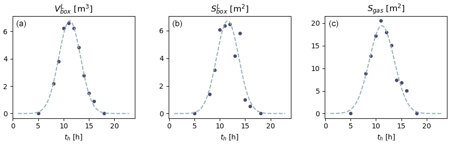
Figure 2 From the left to the right: evolution of (a) $V_{\mathrm{box}}^L$, (b) $S_{\mathrm{box}}^L$ and (c) S_gas with GMT hour. The solid circles denote the values estimated numerically, and the dashed lines are the Gaussian laws they allow for the inference of. These parameterizations are representative of the time period (27 to 31 October) and location (Martigues, France) of the experiments.

2.2 Box evolution and exchanges between the boxes

We denote $V_{\mathrm{box}}^L$ and $V_{\mathrm{box}}^G$ as the volumes of the sunlit and shaded boxes, respectively. Accordingly, the total surface of the room S_room=62.7 m² is split into two parts, $S_{\mathrm{box}}^L$ and $S_{\mathrm{box}}^G$. Their evolution through the day is constrained by the relationships

$$\begin{array}{}\text{(10)}& \begin{array}{rl}{V}_{\mathrm{room}}& =V_{\mathrm{box}}^L+V_{\mathrm{box}}^G,\\ S_{\mathrm{room}}& =S_{\mathrm{box}}^L+S_{\mathrm{box}}^G.\end{array}\end{array}$$

Hourly values of $V_{\mathrm{box}}^L$ and $S_{\mathrm{box}}^L$ were estimated by modelling the solar flux in the room (Tlili et al., 2021). The position of the sun and extrapolation of its beams from the windows were assessed using the Revit 2018 software; the irradiated surface and beam volume were then calculated by vertical and horizontal projections of the indoor solar flux using Autocad 2016 (see http://www.autodesk.fr, last access: 12 May 2021, for both software). The evolution of $V_{\mathrm{box}}^L$ and $S_{\mathrm{box}}^L$ as a function of time t_h [h] is inferred from these values by fitting a Gaussian law (Fig. 2):

$$\begin{array}{}\text{(11)}& V_{\mathrm{box}}^L\left(t_{\mathrm{h}}\right)={\displaystyle \frac{A_{\mathrm{v}}}{{\mathit{\sigma }}_{\mathrm{v}}\sqrt{\mathrm{2}\mathit{\pi }}}}{\text{e}}^{-\frac{(t_{\mathrm{h}}-{\mathit{\mu }}_{\mathrm{v}}{)}^{\mathrm{2}}}{\mathrm{2}{\mathit{\sigma }}_{\mathrm{v}}^{\mathrm{2}}}},\end{array}$$

with A_v=36.505 m³ h, σ_v=2.154 h and μ_v=11.199 h,

$$\begin{array}{}\text{(12)}& S_{\mathrm{box}}^L\left(t_{\mathrm{h}}\right)={\displaystyle \frac{A_{\mathrm{b}}}{{\mathit{\sigma }}_{\mathrm{b}}\sqrt{\mathrm{2}\mathit{\pi }}}}{\text{e}}^{-\frac{(t_{\mathrm{h}}-{\mathit{\mu }}_{\mathrm{b}}{)}^{\mathrm{2}}}{\mathrm{2}{\mathit{\sigma }}_{\mathrm{b}}^{\mathrm{2}}}}\end{array}$$

with A_b=36.958 m² h, σ_b=2.1950 h and μ_b=11.555 h. $V_{\mathrm{box}}^G$ and $S_{\mathrm{box}}^G$ are deduced from $V_{\mathrm{box}}^L$ and $S_{\mathrm{box}}^L$ using Eq. (10). We stress that Eqs. (11) and (12) are valid only for the geometry of the room where the measurements were acquired (building orientation and window position) and for the period during which the campaign was performed (end of October).

$S_{\mathrm{box}}^L$ and $S_{\mathrm{box}}^G$ divide the total solid surface of the experimental room, including the walls, window, floor and ceiling. The complement of $S_{\mathrm{box}}^L$ to obtain the total surface of the sunlit box is the same as the complement of $S_{\mathrm{box}}^G$, which is necessary to obtain the total surface of the shaded box. This complement is the surface allowing gas transfer between the boxes and is denoted as S_gas. This latter complement was estimated with the same method as the one used for $V_{\mathrm{box}}^L$ and $S_{\mathrm{box}}^L$ (Tlili et al., 2021), giving (Fig. 2)

$$\begin{array}{}\text{(13)}& S_{\mathrm{gas}}\left(t_{\mathrm{h}}\right)={\displaystyle \frac{A_{\mathrm{g}}}{{\mathit{\sigma }}_{\mathrm{g}}\sqrt{\mathrm{2}\mathit{\pi }}}}{\text{e}}^{-\frac{(t_{\mathrm{h}}-{\mathit{\mu }}_{\mathrm{g}}{)}^{\mathrm{2}}}{\mathrm{2}{\mathit{\sigma }}_{\mathrm{g}}^{\mathrm{2}}}},\end{array}$$

where A_g=120.04 m² h, σ_g=2.4683 h and μ_g=11.154 h.

The variation of mass within the boxes due to the air mixing is proportional to the surface S_gas. This proportionality is expressed by the air exchange constant k_BOX, defined as (Furtaw et al., 1996)

$$\begin{array}{}\text{(14)}& k_{\mathrm{BOX}}^j=u_{\inf }{\displaystyle \frac{S_{\mathrm{gas}}}{V_{\mathrm{box}}^j}},\end{array}$$

where u_inf is the average velocity of air in the room [m s⁻¹]. This velocity was estimated based on a tracer injection experiment and numerical tests (see Sects. 3.2 and 5.1.1).

2.3 Chemical mechanism

Numerical simulations cannot afford the computation of the millions of reactions occurring in real atmospheres. Approximations are required to reduce this complexity and to alleviate computational efforts. Modellers can opt for different types of kinetic chemical mechanisms, depending on the targeted accuracy. In particular, the lumped-species approach allows the use of a reduced number of compounds, with each compound representing several species having similar properties (Gery et al., 1989; Stockwell et al., 1990; Yarwood et al., 2005; Carter, 2010; Goliff et al., 2013), such as reactivity with OH or carbon bounds. A given species can be represented by a single model compound or by the combination of several model compounds. Mendez et al. (2015) compared the concentrations they obtained with this kind of lumped-species model, SAPRC-07 (Carter, 2010), to the concentrations Carslaw (2007) simulated with the detailed chemistry model MCM and concluded that their overall behaviours were consistent with respect to the O₃, NO_x (NO + NO₂) and HO_x (HO + HO₂) variations. Considering that the general dynamics of homogeneous indoor chemistry can be reproduced by semi-explicit models initially developed for outdoor atmospheres, RACM2, which is also a lumped-species-based model, is used in this paper to solve the chemical reactivity.

To introduce the surface chemistry highlighted by laboratory studies but hardly present in current indoor models, the RACM2 scheme is modified to take into account the heterogeneous reactions listed in Table 1. The resulting modified version of the RACM2 scheme comprises 117 species and 389 reactions, among which 34 are photolytic and 38 heterogeneous. To further investigate the reactions highlighted in the Introduction, some surface species are introduced, namely NO_(ad), NO_2 (ad), HONO_(ad) and HNO_3 (ad). These species can either sorb, desorb or react together. HNO_3 (ad) is not allowed to desorb based on the experimental observation that NO₂ hydrolysis never yields gaseous HNO₃ (Finlayson-Pitts et al., 2003). The kinetic constants of desorption and surface reactions are uncertain and are thus considered tuneable parameters. Adsorption and decomposition reactions are modelled by combining transport to the boundary layer and surface adhesion (Mendez et al., 2015; Morrison et al., 2019), as detailed below.

Table 1 Heterogeneous reactions added to the RACM2 model. The symbol χ designates the species that undergo unimolecular decomposition. These species are O₃, NO₃, HNO₄ and H₂O₂. Reactions (S₁), (S₂), (S₃) and (S₄) (surface reactions) are the model equivalent of Reactions (R1), (R3), (R2) and (R4), respectively.

2.4 Deposition and surface reactivity

This section presents the computation of the kinetic constants of the adsorption and decomposition reactions. The local deposition rate $k_{\mathrm{DEP},i}^j$ is modelled as the equivalent of two resistances in parallel, one corresponding to the transport-limited deposition rate $k_{\mathrm{tran},i}^j$ and the other corresponding to the surface adhesion rate $k_{\mathrm{react},i}^j$:

$$\begin{array}{}\text{(15)}& {\displaystyle \frac{\mathrm{1}}{k_{\mathrm{DEP},i}^j}}={\displaystyle \frac{\mathrm{1}}{k_{\mathrm{tran},i}^j}}+{\displaystyle \frac{\mathrm{1}}{k_{\mathrm{react},i}^j}}.\end{array}$$

When $k_{\mathrm{react},i}^j$ is larger than $k_{\mathrm{tran},i}^j$ the species loss is limited by the transport to the surface boundary layer. In contrast, when $k_{\mathrm{tran},i}^j$ is larger than $k_{\mathrm{react},i}^j$, species removal is limited by surface reactivity (Grøntoft and Raychaudhuri, 2004).

2.4.1 Transport-limited deposition rate

The rate constant $k_{\mathrm{tran},i}^j$ can be expressed as

$$\begin{array}{}\text{(16)}& k_{\mathrm{tran},i}^j=v_{\mathrm{trd},i}{\displaystyle \frac{S_{\mathrm{box}}^j}{V_{\mathrm{box}}^j}},\end{array}$$

where v_trd,i is the deposition velocity limited by transport. It is computed using the method of Lai and Nazaroff (2000), following the same approach as Mendez et al. (2017) to model the heterogeneous production of HONO:

$$\begin{array}{}\text{(17)}& v_{\mathrm{trd},i}=v_{\mathrm{trd},i}^{\mathrm{ad}}{u}^{*},\end{array}$$

where $v_{\mathrm{trd},i}^{\mathrm{ad}}$ is a dimensionless deposition velocity whose computation is detailed below, and u^* is the friction velocity defined by

$$\begin{array}{}\text{(18)}& u^{*}={\left(\mathit{\nu }{\left.{\displaystyle \frac{\text{d}U}{\text{d}y}}\right|}_{y=\mathrm{0}}\right)}^{\mathrm{1}/\mathrm{2}},\end{array}$$

with U the mean air velocity parallel to the surface [m s⁻¹], y the distance from the surface [m] and ν the air kinematic viscosity [m² s⁻¹], defined by $\mathit{\nu }=\mathit{\eta }/\mathit{\rho }$ with η the air dynamic viscosity [kg m⁻¹ s⁻¹] and ρ the air volumetric mass [kg m⁻³]. Considering the narrow temperature range encountered in these experiments, ρ is approximated with the ideal gas law. The viscosity η is expressed as a function of temperature T [K] using the semi-empirical Sutherland relationship:

$$\begin{array}{}\text{(19)}& \mathit{\eta }\left(T\right)={\mathit{\eta }}_{\mathrm{0}}{\left({\displaystyle \frac{T}{T_{\mathrm{0}}}}\right)}^{\mathrm{3}/\mathrm{2}}{\displaystyle \frac{T_{\mathrm{0}}+S_{\mathit{\eta }}}{T+S_{\mathit{\eta }}}},\end{array}$$

where the Sutherland's constant for air is S_η=113 K (Kaper and Ferziger, 1972), and ${\mathit{\eta }}_{\mathrm{0}}=\mathrm{1.783}\times {\mathrm{10}}^{-\mathrm{5}}$ kg m⁻¹ s⁻¹ at T₀=288.15 K.

The derivative of U is given by

$$\begin{array}{}\text{(20)}& {\left.{\displaystyle \frac{\text{d}U}{\text{d}y}}\right|}_{y=\mathrm{0}}=\left({\displaystyle \frac{\mathrm{0.074}}{\mathit{\rho }\mathit{\nu }}}\right)\left({\displaystyle \frac{\mathit{\rho }{u}_{\inf }^{\mathrm{2}}}{\mathrm{2}}}\right){\left({\displaystyle \frac{u_{\inf }l}{\mathit{\nu }}}\right)}^{-\mathrm{1}/\mathrm{5}},\end{array}$$

where l is a characteristic length of the room surface, typically $l=(V_{\mathrm{room}}{)}^{\mathrm{1}/\mathrm{3}}$.

As in Mendez et al. (2017), gravity is assumed to be negligible for gases; i.e. the dimensionless deposition velocity $v_{\mathrm{trd},i}^{\mathrm{ad}}$ is the same for horizontal and vertical surfaces. Assuming that the molecule eddy diffusivity equals the fluid turbulent viscosity ν_t in indoor environments, Lai and Nazaroff (2000) showed that

$$\begin{array}{}\text{(21)}& {\displaystyle \frac{\mathrm{1}}{v_{\mathrm{trd},i}^{\mathrm{ad}}}}=\underset{r_{\mathrm{0}}}{\overset{\mathrm{30}}{\int }}\left({\displaystyle \frac{\mathrm{1}}{\frac{{\mathit{\nu }}_t}{\mathit{\nu }}+\frac{D_i}{\mathit{\nu }}}}\right)\text{d}{y}^{\mathrm{ad}},\end{array}$$

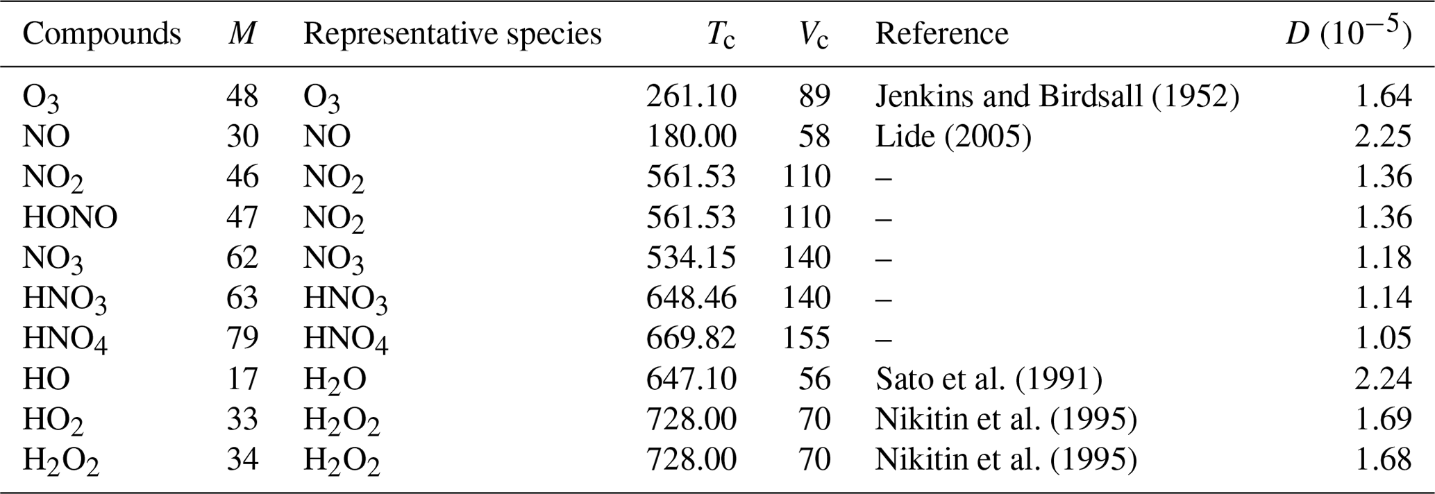
where D_i is the diffusion coefficient of species i [m² s⁻¹], y^ad is the nondimensional distance from the surface and r₀ is the radius of the particle, taken here as zero. The ratio ${\mathit{\nu }}_{\mathrm{t}}/\mathit{\nu }$ is given by Lai and Nazaroff (2000) for several intervals of y^ad. The diffusion coefficient can be estimated based on the species critical temperature T_c [K] and critical volume V_c [cm³ mol⁻¹] following various models. Among all models tested in the comparative study of Ravindran et al. (1979), the model of Chen and Othmer (1962) is the one that showed the best agreement with their experimental data. Considering a species i diffusing in air, this model gives

$$\begin{array}{}\text{(22)}& D_i={\displaystyle \frac{\mathrm{4.3}\times {\mathrm{10}}^{-\mathrm{5}}{\left(\frac{T}{\mathrm{100}}\right)}^{\mathrm{1.81}}\left[\right(M_{\mathrm{air}}+M_i)/(M_{\mathrm{air}}{M}_i){]}^{\mathrm{1}/\mathrm{2}}}{P{\left(\frac{T_{\mathrm{c},\mathrm{air}}{T}_{\mathrm{c},i}}{{\mathrm{10}}^{\mathrm{4}}}\right)}^{\mathrm{0.1406}}{\left[{\left(\frac{V_{\mathrm{c},\mathrm{air}}}{\mathrm{100}}\right)}^{\mathrm{0.4}}+{\left(\frac{V_{\mathrm{c},i}}{\mathrm{100}}\right)}^{\mathrm{0.4}}\right]}^{\mathrm{2}}}},\end{array}$$

where P is the ambient pressure [atm], M_i is the species molar mass and M_air=28.97 g mol⁻¹.

Table 2 presents the diffusion coefficients computed with this method for a list of RACM2 compounds, with the parameters used for this calculation. In this table, T_c and V_c are the critical temperatures and volumes of representative species. The references from which the T_c values are taken are specified. When there is no reference, T_c is computed with the method of Joback and Reid (1987). As experimental values of V_c are difficult to find for a variety of species, all are computed with the method of Joback and Reid (1987).

Jenkins and Birdsall (1952)Lide (2005)Sato et al. (1991)Nikitin et al. (1995)Nikitin et al. (1995)

Table 2 Diffusion coefficients D [m² s⁻¹] and parameters used for their calculation following the procedure described in Sect. 2.4.1: RACM2 molar mass M [g mol⁻¹], critical temperature T_c [K] and critical molar volume V_c [cm³ mol⁻¹] of representative species.

2.4.2 Surface reaction rate

Surface adhesion is modelled with the rate constants $k_{\mathrm{react},i}^j$, which are defined as

$$\begin{array}{}\text{(23)}& k_{\mathrm{react},i}^j={\displaystyle \frac{{\mathit{\gamma }}_i{\mathit{\omega }}_i}{\mathrm{4}}}{\displaystyle \frac{S_{\mathrm{box}}^j}{V_{\mathrm{box}}^j}},\end{array}$$

where γ_i is the uptake coefficient [–] and ω_i the thermal velocity [m s⁻¹] of species i. γ_i is the ratio of collisions of species i with the surface that yield a reaction or simple deposition to the total number of collisions. ω_i depends on the temperature and can be expressed as

$$\begin{array}{}\text{(24)}& {\mathit{\omega }}_i=\sqrt{\mathrm{2.1171}\times {\mathrm{10}}^{\mathrm{4}}{\displaystyle \frac{T}{M_i}}}.\end{array}$$

The uptake coefficient is characteristic of the relationship between the species and the surface. It has been determined experimentally with the paints used in this study for two species, NO₂ and xylene, indicating that uptake coefficients of other species are unknown. The deposition of organic species is beyond the scope of this paper, as organic concentrations are set to the measured values here. The uptake coefficients of NO, HONO and O₃ are uncertain and thus considered tuneable parameters. Since the simulated concentrations of NO₃, HNO₃, HNO₄ and H₂O₂ are low, they are given an infinite uptake for simplicity so that their deposition is only controlled by transport ($k_{\mathrm{DEP},i}^j=k_{\mathrm{tran},i}^j$). By default, the same procedure is applied to the HO₂ radical, noting that when its deposition is neglected, the resulting difference in the average NO_x concentration is of the order of 0.1 µg m⁻³. Likewise, the deposition of the OH radical is considered negligible compared with its consumption by homogeneous reactivity (Sarwar et al., 2002). There is evidence that low-volatility species sorbed on surfaces can be subject to OH oxidation (Alwarda et al., 2018), but chemical variations of surface films caused by indoor oxidants are beyond the scope of this work.

2.4.3 Parameterization of ${\mathit{\gamma }}_{{\mathrm{NO}}_{\mathrm{2}}}$

The uptake coefficient ${\mathit{\gamma }}_{{\mathrm{NO}}_{\mathrm{2}}}$ was measured in various laboratory conditions by Gandolfo et al. (2015, 2017). This section explains how parameterizations are inferred from these measurements and how they are used to calculate ${\mathit{\gamma }}_{{\mathrm{NO}}_{\mathrm{2}}}$ as a function of ambient conditions.

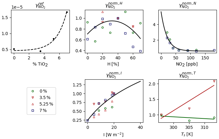
The measurements made as a function of the relative humidity, denoted as H, are normalized by the measurement made at H_ref=40 %. This gives the following using a polynomial fitting:

$$\begin{array}{}\text{(25)}& {\mathit{\gamma }}_{{\mathrm{NO}}_{\mathrm{2}}}^{\mathrm{norm},H}\left(H\right)=\sum _{k=\mathrm{0}}^{\mathrm{2}}{a}_k{H}^k,\end{array}$$

where a₀=0.706, $a_{\mathrm{1}}=\mathrm{1.50}\times {\mathrm{10}}^{-\mathrm{2}}$ and $a_{\mathrm{2}}=-\mathrm{2.31}\times {\mathrm{10}}^{-\mathrm{4}}$.

Considering that ${\mathit{\gamma }}_{{\mathrm{NO}}_{\mathrm{2}}}$ varies with the NO₂ concentration in the room, measurements were made as a function of the NO₂ concentration in parts per billion (ppb), denoted as N. By normalizing these measurements by the measurement made at N_ref=40 ppb, an exponential fitting gives

$$\begin{array}{}\text{(26)}& {\mathit{\gamma }}_{{\mathrm{NO}}_{\mathrm{2}}}^{\mathrm{norm},N}\left(N\right)=\mathrm{118.06}{\exp }^{\frac{-(N+\mathrm{64.52})}{\mathrm{20.41}}}+\mathrm{0.61}.\end{array}$$

Measurements were also made as a function of the light intensity irradiating the surface, denoted as I. The light intensity produced by the reactor covered a spectrum ranging from 340 to 400 nm. Because the paint photocatalytic effect reaches saturation above a certain light threshold, a function type that does not increase too much at high intensity is chosen to express ${\mathit{\gamma }}_{{\mathrm{NO}}_{\mathrm{2}}}^{\mathrm{norm},I}$. Using the measurements normalized by the measurement made at I_ref=8.5 W cm⁻², a logarithmic fitting gives

$$\begin{array}{}\text{(27)}& {\mathit{\gamma }}_{{\mathrm{NO}}_{\mathrm{2}}}^{\mathrm{norm},I}\left(I\right)=\ln (I+\mathrm{19.63})-\mathrm{2.74}.\end{array}$$

Contrary to the other measurements, the measurements made as a function of temperature were performed at I=20 W m⁻². By dividing the measurements as a function of I by the measurement made at I=20 W m⁻², a relationship similar to Eq. (27) is obtained and denoted as ${\mathit{\gamma }}_{{\mathrm{NO}}_{\mathrm{2}}}^{\mathrm{norm},I_{\mathrm{2}}}$. By multiplying the measurements as a function of temperature by ${\mathit{\gamma }}_{{\mathrm{NO}}_{\mathrm{2}}}^{\mathrm{norm},I_{\mathrm{2}}}\left(I_{\mathrm{ref}}\right)$, these measurements are brought to the same conditions of irradiance as the other measurements. They are then divided by the measurement made at T_ref=296 K. Finally, a polynomial fitting gives

$$\begin{array}{}\text{(28)}& {\mathit{\gamma }}_{{\mathrm{NO}}_{\mathrm{2}}}^{\mathrm{norm},T}\left(T\right)=b_{\mathrm{1}}{T}_{\mathrm{s}}\left(T\right)+b_{\mathrm{0}},\end{array}$$

where $b_{\mathrm{0}}=-\mathrm{17.62}$ and $b_{\mathrm{1}}=\mathrm{6.25}\times {\mathrm{10}}^{-\mathrm{2}}$ K⁻¹ for the paint containing 3.5 % TiO₂. The values b₀=1 and b₁=0 are preferred for the reference paint, considering that the observed decreasing trend falls within the measurement's uncertainty. T_s is the temperature of the surface of paint [K]. In a real room, T_s depends on a variety of factors, including location, season, orientation, ambient temperature and surface coating (Shen et al., 2011). For the simulations, T_s is set such that T_s=T in the shaded box and $T_{\mathrm{s}}=\mathrm{1.2}\times (T-\mathrm{273.15})+\mathrm{273.15}$ in the sunlit box.

The ${\mathit{\gamma }}_{{\mathrm{NO}}_{\mathrm{2}}}$ at a given set of parameters H, N and T is calculated from the reference uptake coefficient ${\mathit{\gamma }}_{{\mathrm{NO}}_{\mathrm{2}}}^{\mathrm{ref}}$ measured at T_ref=296 K, H_ref=40 %, I_ref=8.5 W m⁻² and N_ref=40 ppb, according to

$$\begin{array}{}\text{(29)}& \begin{array}{rl}{\mathit{\gamma }}_{{\mathrm{NO}}_{\mathrm{2}}}(H,N,T)& ={\mathit{\gamma }}_{{\mathrm{NO}}_{\mathrm{2}}}^{\mathrm{ref}}{\mathit{\gamma }}_{{\mathrm{NO}}_{\mathrm{2}}}^{\mathrm{norm},N}\left(N\right){\mathit{\gamma }}_{{\mathrm{NO}}_{\mathrm{2}}}^{\mathrm{norm},H}\left(H\right)\\ & \cdot {\mathit{\gamma }}_{{\mathrm{NO}}_{\mathrm{2}}}^{\mathrm{norm},T}\left(T\right).\end{array}\end{array}$$

The parameterization ${\mathit{\gamma }}_{{\mathrm{NO}}_{\mathrm{2}}}^{\mathrm{norm},I}$ is not considered in Eq. (29), given that it was established based on measurements with a light spectrum ranging from 340 to 400 nm and that the measurements presented in this paper were obtained with a light spectrum starting from 395 nm.

The dependence of ${\mathit{\gamma }}_{{\mathrm{NO}}_{\mathrm{2}}}^{\mathrm{ref}}$ with the percentage of TiO₂ nanoparticles contained by the paint and the parameterizations of ${\mathit{\gamma }}_{{\mathrm{NO}}_{\mathrm{2}}}^{\mathrm{norm}}$ are presented in Fig. 3. ${\mathit{\gamma }}_{{\mathrm{NO}}_{\mathrm{2}}}^{\mathrm{ref}}$ increases with the percent of TiO₂, but the values at 0 % and 3.5 % are very close. In the simulations, ${\mathit{\gamma }}_{{\mathrm{NO}}_{\mathrm{2}}}^{\mathrm{ref}}=\mathrm{5}\times {\mathrm{10}}^{-\mathrm{6}}$ is used for both paints and for the surface that is not covered by paint (floor, ceiling, rest of the walls).

Figure 3 Evolution of ${\mathit{\gamma }}_{{\mathrm{NO}}_{\mathrm{2}}}$. The dots denote measurements, and the open symbols denote normalized measurements (see text for details). The solid lines denote the parameterization as a function of H, N, I and T_s (Eqs. 25–28).

2.5 Desorption rates

According to Ramazan et al. (2004), water competes with HONO_(ad) for surface sites and displaces HONO_(ad) towards a gas phase as the surface water vapour increases. The higher the water vapour is, the more HONO_(ad) desorbs. On the other hand, the lower the water vapour is, the more HONO_(ad) is available to react with other sorbed species such as NO. In this study, it is assumed that the same holds for the other adsorbed compounds. As no information on the surface water concentration is available, the desorption reactions are parameterized as a function of the room humidity. The desorption kinetic constants are defined as

$$\begin{array}{}\text{(30)}& k_{i,\text{(ad)}}={\mathit{\alpha }}_i{k}_{\mathrm{H},i}{n}_{{\mathrm{H}}_{\mathrm{2}}\mathrm{O}},\end{array}$$

where $n_{{\mathrm{H}}_{\mathrm{2}}\mathrm{O}}$ is the number of water molecules in the room computed from the water mass fraction (absolute humidity), k_H,i is the Henry's law constant of compound i [bar mol kg⁻¹] and α_i is a tuneable variable [kg bar⁻¹ mol⁻¹ s⁻¹ molec.⁻¹]. The value of k_H,i characterizes the compound affinity for water. The temperature range of these experiments (see Table 3) is considered sufficiently narrow to neglect the dependence of k_H,i on temperature. At T=298.15 K, $k_{\mathrm{H},\mathrm{NO}}=\mathrm{0.0019}$ bar mol kg⁻¹, $k_{\mathrm{H},{\mathrm{NO}}_{\mathrm{2}}}=\mathrm{0.012}$ bar mol kg⁻¹ and $k_{\mathrm{H},\mathrm{HONO}}=\mathrm{49}$ bar mol kg⁻¹ (, ). For simplicity, in the rest of this paper, we will use $k_{i,\text{(ad)}}^{\prime }={\mathit{\alpha }}_i{k}_{\mathrm{H},i}$.

2.6 Photolysis

In all indoor models presented in the Introduction, light was assumed to have two origins: sunlight and artificial light. Using the indoor light intensity recommended for reading purposes, Sarwar et al. (2002) assumed that each light source accounted for 50 % of the total light and accordingly combined spectral power distributions obtained from the literature to obtain the total spectral distribution. Nazaroff and Cass (1986), Mendez et al. (2015), and Carslaw (2007) computed their own outdoor photon fluxes and applied attenuation factors to account for window filtration. Carslaw (2007) and Mendez et al. (2015) used the same indoor light fluxes as Nazaroff and Cass (1986) and started with the same attenuation factors before varying them.

Whereas light intensity can be considered homogeneous in direct light whatever the distance from the window (Kowal et al., 2017), it decreases rapidly moving away from the direct sunlight (Gandolfo et al., 2016). The distribution of light intensity in the shaded volume is strongly location-specific and thus hard to predict. However, light intensity in the shaded volume is much lower than the intensity of direct light; therefore, the impact of the photolytic reactions occurring in the shaded volume is minor compared with that occurring in the sunlit volume. As an approximation, the photolytic constants in the shaded box are computed using a unique actinic flux that was measured close to the area illuminated by the sunlight. This model does not represent the light decrease when moving away from the window because only two boxes are considered: shaded and sunlit.

Let ζ be the indoor actinic flux [photons cm⁻² s⁻¹ nm⁻¹] measured at t=t_ref. Let λ_min and λ_max be the minimum and maximum wavelengths of the light spectrum [nm]. The photolytic constants associated with this actinic flux are given by (Nazaroff and Cass, 1986)

$$\begin{array}{}\text{(31)}& J_i^{\mathrm{ref}}=\underset{{\mathit{\lambda }}_{\min }}{\overset{{\mathit{\lambda }}_{\max }}{\int }}\mathit{\zeta }\left(\mathit{\lambda }\right){\mathit{\kappa }}_i\left(\mathit{\lambda }\right){\mathit{\varphi }}_i\left(\mathit{\lambda }\right)\text{d}\mathit{\lambda },\end{array}$$

where $J_i^{\mathrm{ref}}$ is the photolytic constant of species i [photons cm⁻² s⁻¹] at t=t_ref, κ_i the species cross section [–] and ϕ_i the species quantum yield [–]. The actinic flux used to calculate $J_i^{\mathrm{ref}}$ in the indirect light was measured at t_ref=11:00 (GMT) on 27 October (Experiment 1), and the one used to calculate $J_i^{\mathrm{ref}}$ in the direct light was measured at t_ref=11:00 (GMT) on 29 October (Experiment 3). The light spectrum starts at λ_min=390 nm in the direct light and λ_min=394 nm in the indirect light. Both spectra end at 660 nm.

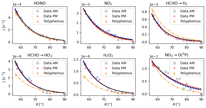
Figure 4 Photolysis rates as a function of zenith angle. The symbols ◦ and + denote the experimental rates acquired on 30 October in the morning and in the afternoon. The blue and red dashed lines are their parameterization using Eq. (32). The black solid line is the curve obtained by fitting the data from both the morning and those from the afternoon. The △ symbols are the photolysis rates calculated with Eq. (31) with the cross sections and quantum yields taken from Polyphemus. The yellow dash-dotted line is the deriving evolution of J with θ according to Eq. (34).

To account for the evolution of the photolytic constants with the time of day, a parameterization is inferred from the HONO, NO₂, HCHO, H₂O₂ and NO₃ photolytic rates measured by a spectroradiometer in direct light on 30 October with windows that did not cut UV rays (Fig. 4):

$$\begin{array}{}\text{(32)}& J_i\left(\mathit{\theta }\right)=A_i{\exp }^{\frac{-(\mathit{\theta }-C)}{B}},\end{array}$$

where θ is the zenith angle and J_i is the photolytic constant of species i as a function of θ. The evolution of θ with the hour of the day is presented in Fig. 5. The curves fitting the J_i rates measured in the morning and those fitting the ones measured in the afternoon are superimposed in Fig. 4, indicating no hysteresis. For each compound, the values of B and C are very close, with an average of B=10.7 and C=50. For a given compound, the prefactor A is given by

$$\begin{array}{}\text{(33)}& A_i=J_i^{\mathrm{ref}}{\exp }^{\frac{{\mathit{\theta }}_{\mathrm{ref}}-C}{B}},\end{array}$$

where θ_ref is the zenith angle corresponding to t_ref. This yields

$$\begin{array}{}\text{(34)}& J_i\left(\mathit{\theta }\right)=J_i^{\mathrm{ref}}{\exp }^{\frac{-(\mathit{\theta }-{\mathit{\theta }}_{\mathrm{ref}})}{B}}.\end{array}$$

Equation (34) is plotted in Fig. 4 using the $J_i^{\mathrm{ref}}$ calculated with the ϕ and κ values available for the RACM2 chemical mechanism (Kim et al., 2009) in the Polyphemus air-quality modelling platform. We observe reasonable agreement between the measured and calculated photolytic rates.

Figure 5 Zenith angle θ as a function of the hour of the day on 27 October at latitude 43.41^∘ and longitude 5.06^∘ (Martigues area). The ◦ symbols denote the hours of the J_i measurements by the spectroradiometer.

2.7 Numerical resolution

The simulations start and end at the times fixed by the user (see Sect. 3.1). The time step Δt of the main loop of time in the programme is set to 100 s. It corresponds to an input–output time step: at the beginning of each iteration of the main loop, input data such as temperature, humidity and outdoor concentrations are read from a file, and at the end of each iteration, the concentrations are written to a file. Variables characterizing the environment and the source and sink terms are also initialized and updated in the main loop, namely box volumes and surfaces (Eqs. 10–12), box air exchange (Eq. 14), ventilation, supply from outdoors, and emissions.

The resolution of Eq. (4) is performed using operator splitting: the evolution of the concentrations due to emissions, air exchanges between boxes, and between the room and the outside is first solved using the explicit trapezoidal rule (ETR), which is an explicit second-order solver corresponding to a two-stage Runge–Kutta method (Ascher and Petzold, 1998). The time step is adapted as described in Sartelet et al. (2006): each main time step Δt of 100 s is decomposed in sub-time steps δt_k determined by the ETR method, such as $\mathrm{\Delta }t={\sum }_k\mathit{\delta }{t}_k$. After each sub-time step δt_k, the third and last terms of the right-hand side of Eq. (4) are solved together. The evolution of the concentrations due to homogeneous and heterogeneous reactions and deposition is computed using the Rosenbrock 2 (ROS2) algorithm (Rosenbrock, 1963; Sandu et al., 1997), with time steps automatically adapted between δt_k and δt_k+1 by the ROS2 algorithm.

In this paper, the VOC concentrations are assigned to their experimental values at each iteration of the main loop. By imposing the VOC concentrations at each main iteration, no drift is observed between experimental and calculated values, indicating that the characteristic time of their evolution caused by chemical reactivity, sources and sinks is lower than the model time step Δt. Note that this is not the case with more reactive species, such as NO and NO₂, which may evolve significantly between two iterations.

3 Input data and parameters for model evaluation

3.1 Measurements used as input and model–measurement comparisons

Three experiments were conducted with anti-UV windows in an office room in a new building situated in the suburban area of Martigues (France) less than 6 months after its construction. The first one was conducted without any paint board (“naked” walls), the second one with walls covered by the reference paint and the third one with walls covered by the 3.5 % TiO₂ paint. The complete description of these experiments is provided by Gandolfo et al. (2021) (see also Gandolfo, 2018). This section provides a brief introduction of the data used in this paper.

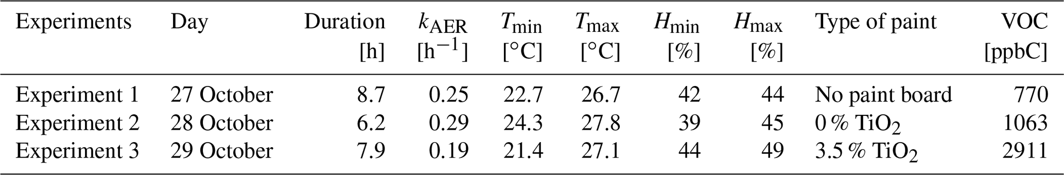
The room was ventilated before each experiment. The start time of the simulation is chosen to match the beginning of the VOC concentration increase caused by the closing of the windows. When the windows were closed, the air exchange rate k_AER was determined by continued analysis of an inert gaseous tracer (CO₂) injected into the room at the beginning of the experiment. For a given day, the measured k_AER values were almost constant, which allows running the simulations with a daily average value for each experiment. Indoor temperature and humidity were measured every 10 s. They are involved in the computation of air viscosity, friction velocity, species diffusivities, thermal and deposition velocities, and uptake values. The durations of the experiments, average ventilation rates, minimum and maximum temperatures and humidities, and average total VOC concentrations recorded are summarized in Table 3.

Table 3 Parameters of the experiments: total duration, k_AER, minimum and maximum temperature and humidity, type of paint, average total VOC concentration.

Outdoor concentrations, used as model input, are estimated by linear interpolation of outdoor measurements. VOCs were measured with a PTR-ToF-MS (proton transfer reaction time-of-flight mass spectrometer) equipped with a motorized valve rotating alternatively for 5 min outdoors and 10 min indoors, providing an outdoor VOC measurement every 15 min. The O₃ outdoor concentrations were measured at a rate of one measurement per minute. The NO and NO₂ outdoor concentrations were recorded on a quarter-hourly basis by the regional air-quality network AtmoSud at a station located approximately 1.5 km away and for which the NO_x concentrations are expected to be representative of the concentrations close to the building. Outdoor HONO, OH and HO₂ were not measured. They are thus fixed at a constant and realistic value of 20 ppt for HONO, 10⁶ molecules per cubic centimetre (molec. cm⁻³) for OH and 10⁸ molec. cm⁻³ for HO₂ (Holland et al., 2003).

Due to the PTR-ToF-MS valve rotations, an indoor VOC measurement every 15 min was performed with a shift of 5 and 10 min with the previous and subsequent outdoor VOC measurement, respectively. Indoor NO_x was measured by chemiluminescence, HONO using a LOPAP (long-path absorption photometer) and O₃ by spectrophotometry. All instruments were placed in a separate room. The presence of instruments in the experiment room would have increased the surface available for heterogeneous reactivity in a hardly quantifiable way, thus introducing uncertainty. O₃ was captured at the centre of the room at a rate of one measurement per minute. NO_x was measured every second and HONO every 15 s. The modelled O₃, HONO and NO_x are compared with these experimental records. The sources of these species are infiltration from the outdoors and chemical reactivity; therefore, no emission rate is considered for them.

3.2 Model parameters

The inorganic species measurements are considered a benchmark to estimate the model's undetermined parameters. These parameters are the building filtration factor f, the kinetic constants of the surface and desorption reactions (see Table 1), the uptake coefficients of O₃, NO and HONO, the initial concentrations of the surface species NO_(ad), NO_2 (ad), HONO_(ad) and HNO_3(ad), and, to a lesser extent, the velocity of air in the room u_inf.

The velocity of air in the room is assessed by measuring the homogenization time of a tracer gas injection. A styrene injection indicated that this velocity could range between 0.05 and 0.4 m s⁻¹. Furtaw et al. (1996) and references therein have suggested the same admissible bounds for this parameter, with a value of 0.15 m s⁻¹ identified as a reference for comfortable indoor conditions (McQuiston et al., 2004). In the experiments listed in Table 3, two fans were placed on both sides of the room, providing active air mixing and thus a u_inf value likely exceeding 0.15 m s⁻¹.

The building filtration factor controls the fluxes of outdoor pollutants that enter the room through the cracks and gaps of the building's structure. Its value derives from the routes available for transport and from the pollutant's reactivity with the materials of the building's enclosure assembly, which can scavenge components that are infiltrating (Zhao et al., 2019). Its value is component-specific and ranges from 0 (no intrusion) to 1. In the absence of measurements, it is omitted or taken as unity in most models (Sarwar et al., 2002; Carslaw, 2007; Mendez et al., 2015). For the present study, no filtration factor measurement was made. The filtration factor is thus considered to be completely undetermined. For convenience, the same value is used for all compounds.

Among the surface species introduced in this model, NO₂ is the only one whose uptake value was determined experimentally; the other ones are adjusted by the user. The value of γ_NO is expected to be low given that all models consider a zero deposition velocity for NO, following Nazaroff and Cass (1986). The uptake coefficients provided for NO, HONO and O₃ are supposed to be the uptake values at T_ref=296 K, H_ref=40 % and I_ref = 8.5 W m⁻² at a concentration of 40 ppb. Their variations are parameterized with the same relationships as the ones obtained for NO₂ (see Sect. 2.4.3).

Another element that can be considered uncertain is the stoichiometry of the NO₂ hydrolysis reaction. Generally, it is assumed that HONO_(ad) and HNO_3(ad) are formed with equal yields (Febo and Perrino, 1991). Finlayson-Pitts et al. (2003) measured the yields of gas-phase HONO, NO and N₂O, expressed relative to the measured losses of NO₂ in the course of NO₂ heterogeneous hydrolysis experiments in laboratory systems. The measured yield of HONO was less than 50 % of the NO₂ loss, but the NO yield was attributed to secondary reaction of the HONO formed by NO₂ on surfaces. The sum of the yields of gas-phase HONO and secondary reaction products such as NO was close to 50 %, but not exactly 50 %. Furthermore, there is, to the authors' knowledge, no available measurement of the HNO₃ yield, since no HNO₃ production is observed in the gas phase in the course of this type of experiment. By using NO${}_{\mathrm{2}\text{(ad)}}\to {\mathit{\beta }}_{{\mathrm{HNO}}_{\mathrm{3}}}$ HNO_3(ad)+β_HONO HONO_(ad), small variations of ${\mathit{\beta }}_{{\mathrm{HNO}}_{\mathrm{3}}}$ and β_HONO are considered, with the constraint that ${\mathit{\beta }}_{{\mathrm{HNO}}_{\mathrm{3}}}+{\mathit{\beta }}_{\mathrm{HONO}}=\mathrm{1}$, to ensure nitrogen conservation.

3.3 Initial conditions

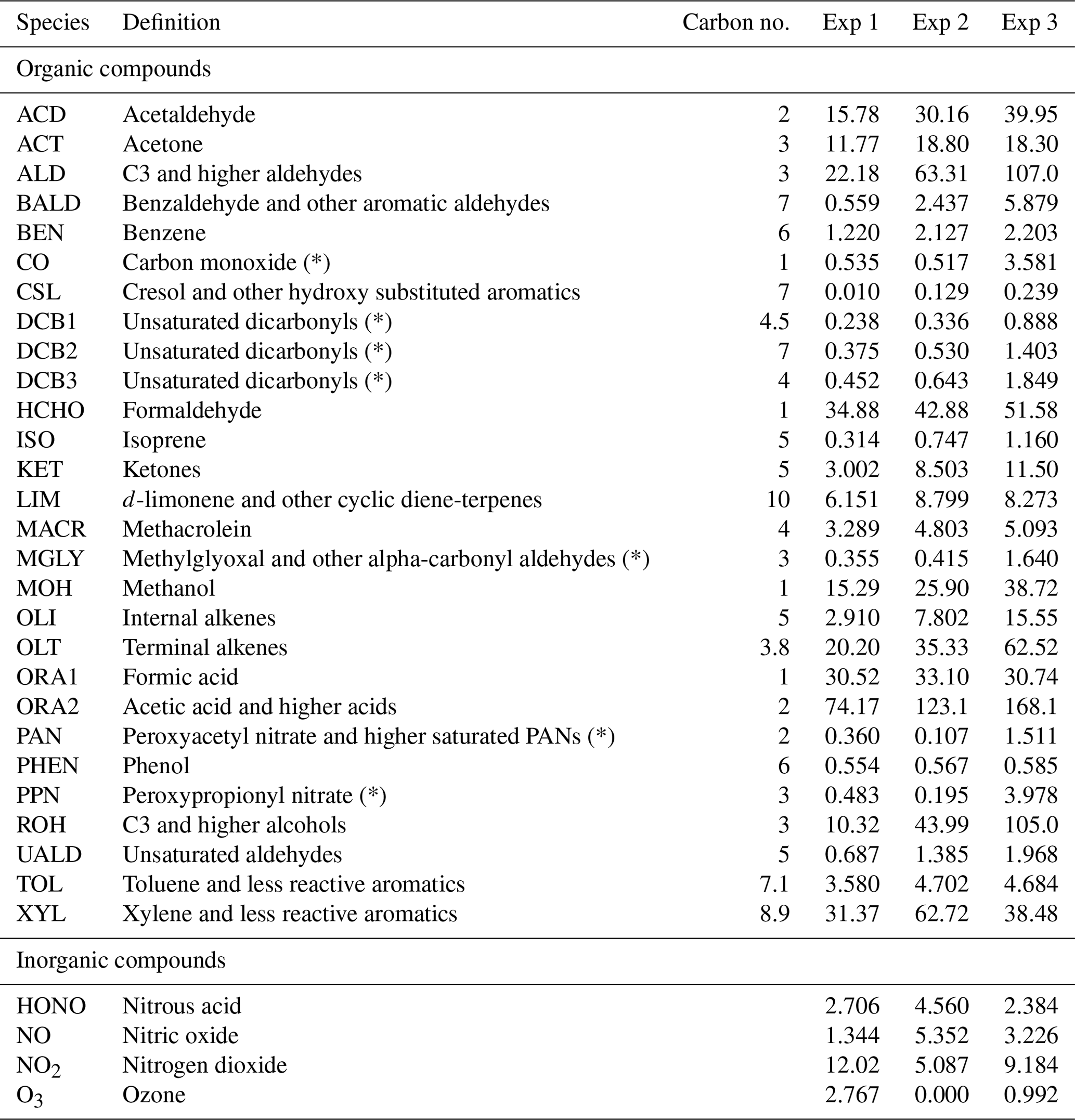
According to Nazaroff and Cass (1986), simulations can be sensitive to changes in initial conditions over a characteristic time period that can be considered proportional to the inverse of the air exchange rate. When the simulated period extends over several days (Sarwar et al., 2002; Carslaw, 2007; Courtey et al., 2009), the influence of initial conditions can be neglected. In the present study, the air renewal time ($k_{\mathrm{AER}}^{-\mathrm{1}}$), i.e. the minimum time needed to break free from the initial conditions, represents about half of the simulated periods, which thus requires careful setting of the initial concentrations. The RACM2 organic and inorganic compound concentrations are initialized using the concentrations measured at the start time of the experiments, which are shown in Table 4. However, this is not sufficient to initiate the radical's chemistry, which is influenced by a variety of species, including VOCs that were not measured because they were unidentifiable or under the detection limit of the PTR-ToF-MS. Without proper initialization, the chemistry of radicals is absent from the start of the experiment, which damages the inorganic chemistry and thus the comparison between the model and experiments.

Table 4 List of the RACM2 compounds initialized. The table shows the definition, carbon valence and concentrations at the start of the experiments; concentrations are in micrograms per cubic metre (µg m⁻³). Compounds marked with a symbol (*) were not measured experimentally, but were estimated based on simulations to assess their importance regarding initial conditions (see Sect. 3.1).

To assess the initial concentrations of the species that were not detected, a simulation is run while forcing the organic and inorganic compounds to follow their measured values for a duration d_init. Then, a new simulation is launched by assigning the concentrations obtained at the end of d_init to the compounds that were not measured; the other ones are again initiated using the concentrations measured at the start time of the experiments, which are shown in Table 4. With these new initial conditions, the simulated concentrations of radicals are higher than in the initial simulation, as shown by the variations in the NO_x profiles (see Figs. B1–B3 in the Appendix), which are strongly influenced by the concentrations of radical species. This procedure is repeated iteratively. The correspondence between these simulation runs and the NO_x concentrations is assessed by computing the mean normalized gross error (MNGE) over the first 5000 s of the simulation run. The time d_init is not the same for all experiments but is fixed for a given experiment. This time is chosen depending on the rate of convergence of the simulation runs, which increases with increasing k_AER and decreases with increasing VOC concentration (see Table 3). This duration amounts to 2300 s for Experiment 1, 1900 s for Experiment 2 and 4200 s for Experiment 3. Proper initial concentrations are considered to be achieved when the MNGE with respect to NO and NO₂ stabilizes or reaches a minimum.

In Fig. 6, the simulations performed by initializing only the compounds that were quantified experimentally are labelled as “without radical initialization”. The simulations performed by initializing all species, following the procedure explained above, are labelled as “full initialization”. The full initialization completely modifies the NO and HONO profiles, as well as the first part of the NO₂ profile.

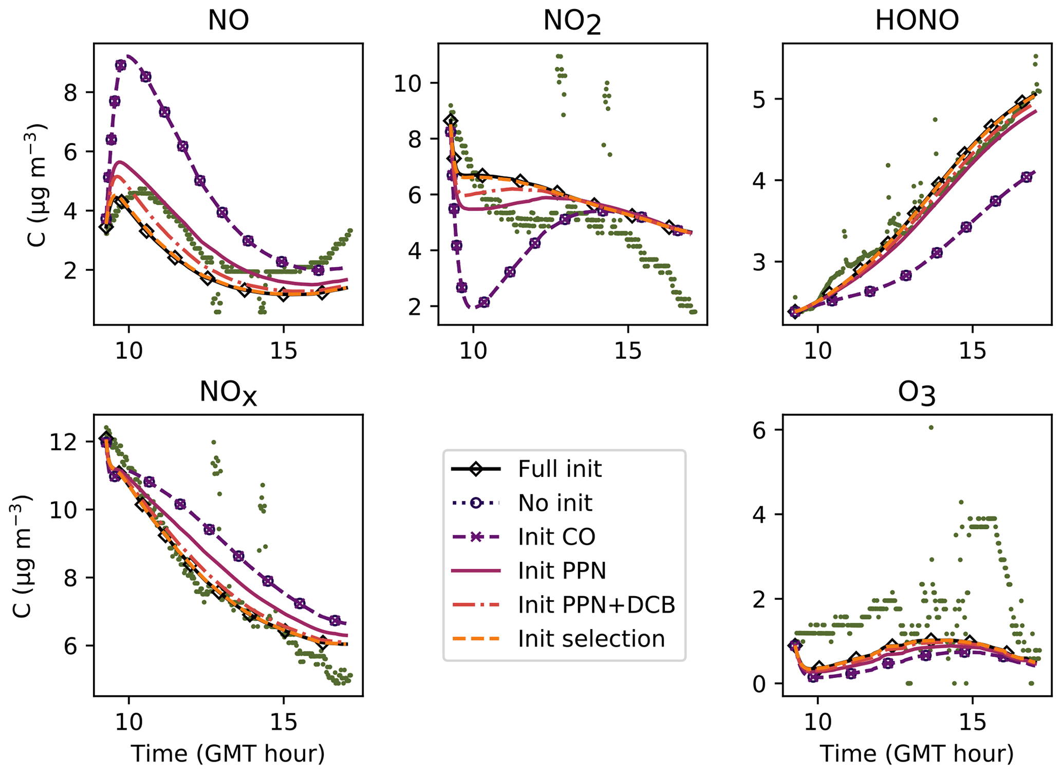
Figure 6 Inorganic concentration profiles for different initial conditions. The dots denote the experimental measurements (Experiment 3). “No init” means that all the compounds which were not detected during the campaign are a given a zero concentration at the start of the simulation. “Full init” means that all the compounds are initialized, even those which were not experimentally detected (see text for details). “Init CO” is like “No init” but with CO initialized. “Init PPN” is like “No init” but with PPN initialized . “Init PPN+DCB” is like “No init” but with PPN, DCB1, DCB2 and DCB3 initialized. “Init selection” is like “No init” but with PPN, DCB1, DCB2, DCB3, MGLY and PAN initialized. The curves corresponding to “Full init” and “Init selection” are close to being superimposed.

It is clear that all compounds do not contribute equally to the radical chemistry. Namely, the initialization of compound PPN (peroxyl propionyl nitrate) bridges about half of the gap between the simulations without radical initialization and the simulations with full initialization. Among the 68 RACM2 compounds that were not detected during the experiments but for which the model predicts a non-zero concentration, only six need to be initialized to attain proper radical chemistry. These are PAN (peroxyacetyl nitrate and higher saturated PANs), MGLY (methylglyoxal and other alpha-carbonyl aldehydes), DCB1, DCB2 and DCB3 (unsaturated dicarbonyls), and PPN. The initialization of these compounds in addition to the species measured experimentally provides the same effect on the inorganic compounds as the full initialization.

It can be inferred from this section that a careful assessment of the initial concentrations, including for compounds that were not experimentally detected, is mandatory for this type of study.

4 Reference simulations

The parameters presented in Sect. 3.2 are calibrated to reach the best correspondence between experimental data and simulations as possible. The filtration factor f varies between experiments depending on wind conditions. The air-mixing velocity and the stoichiometry of the NO₂ heterogeneous hydrolysis do not vary between experiments. However, the values of the surface kinetic reaction rates, desorption rates and uptake coefficients may vary between experiments because of differences in wall covering. Therefore, the parameters are first adjusted for each experiment independently. This set of optimized parameters is denoted as Set 1. To determine parameter values usable in a wide range of conditions, the parameters are then varied to use the same values of surface kinetic reaction rates k_S for all experiments, but letting the desorption rates $k_{i,\text{(ad)}}^{\prime }$ vary with experiment. This leads to the set of parameters denoted as Set 2. Finally, the set of parameters denoted as Set 3 corresponds to parameters adjusted to use the same values for all experiments. Note that in the first experiment, the desorption constant $k_{\mathrm{NO}\left(\mathrm{ad}\right)}^{\prime }$ still requires a lower value than the common one. In the rest of this paper, “reference simulations” will denote the simulations obtained with the Set 3 parameter values, while “optimized simulations” will denote the simulations obtained with the Set 1 parameter values. All parameter values are listed in Table 5.

Figures 7, 8 and 9 present the three sets of simulations for the three experiments. In these graphs, the solid lines denote the concentrations simulated in the sunlit box and the dashed lines the concentrations in the shaded box. These two curves are identical. The NO, NO₂ and NO_x outlying dots observed at 10:20 and 12:10 for Experiment 1, as well as 12:45 and 14:20 for Experiment 3, are sporadic outdoor measurements and are thus not simulated by the model. During Experiment 1, an artificial NO₂ injection of about 56 ppb (including a few parts per billion of NO) was performed at 13:30. The simulated NO and HONO outbreaks generated by this NO₂ injection exceed the concentrations measured experimentally; they arise from surface chemistry and cannot be cancelled out by changing the parameters without damaging the simulated profiles before the injection.

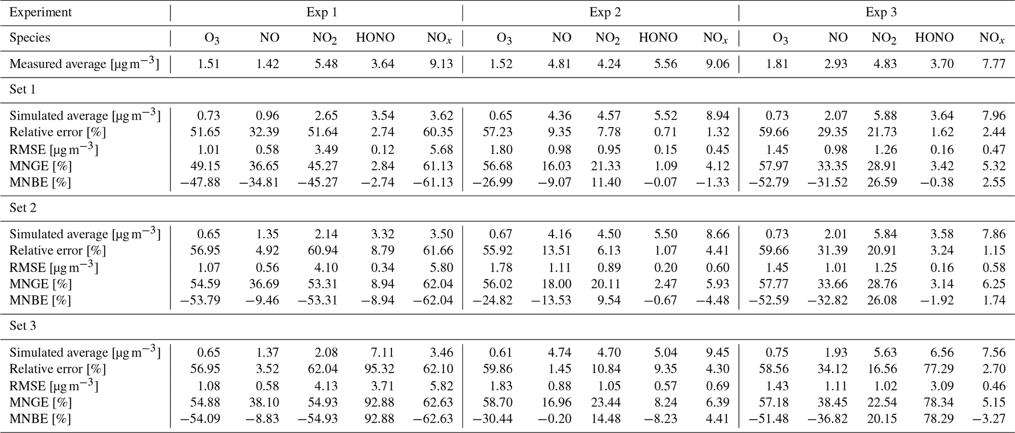
The similarity between simulations and experiments is quantified by computing, for the four modelled inorganic compounds, the relative error between the average measured and simulated concentrations, the root mean square error (RMSE), the mean normalized gross error (MNGE), and the mean normalized bias error (MNBE), as presented in Table 6. For the first experiment, these indicators are computed over the period preceding the NO₂ injection only.

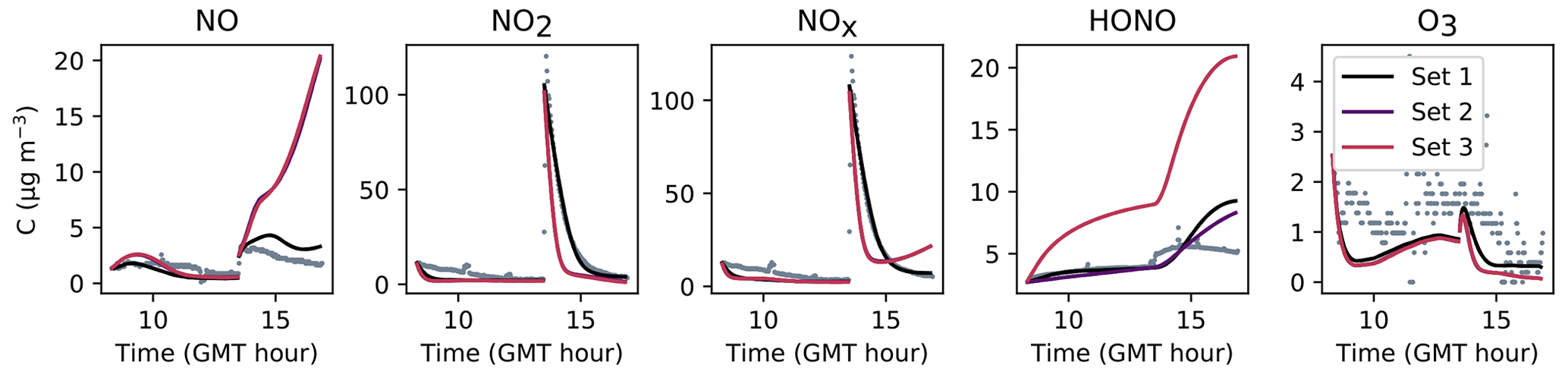
Figure 7 Simulation of Experiment 1 for the three sets of parameters. The dots denote the experimental records. The concentrations simulated in the sunlit box (solid lines) and the concentrations simulated in the shaded box (dashed lines) are superimposed.

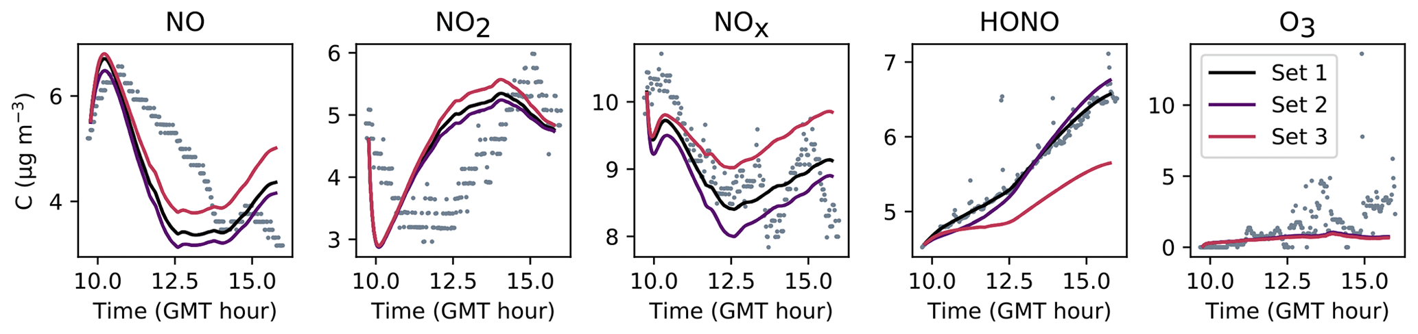
Figure 8 Simulation of Experiment 2 for the three sets of parameters. The dots denote the experimental records. The concentrations simulated in the sunlit box (solid lines) and the concentrations simulated in the shaded box (dashed lines) are superimposed.

Figure 9 Simulation of Experiment 3 for the three sets of parameters. The dots denote the experimental records. The concentrations simulated in the sunlit box (solid lines) and the concentrations simulated in the shaded box (dashed lines) are superimposed.

The NO_x concentration is modelled very well in Experiments 2 and 3, with an MNGE of 4 %–6 %. For NO₂, the MNGE is about 22 % in Experiment 2, while it reaches about 28 % in Experiment 3. Regarding NO, the MNGE is about 17 % in Experiment 2 and 35 % in Experiment 3. In Experiment 1, the NO_x concentrations are systematically underestimated, with an MNBE of −62 % in the first part of the simulation. In the second part, the NO₂ decay following the NO₂ injection is replicated very well using the optimized parameters. For all experiments and all sets of parameters, O₃ is underestimated with a relative error ranging between 50 % and 60 %. HONO exhibits excellent statistics for Set 1 and Set 2, with an MNGE from 1 % to 9 % in the three experiments. However, using the common parameters (Set 3), HONO is underestimated in Experiment 2 (−8 % MNBE) and strongly overestimated in Experiments 1 and 3 (94 % and 78 % MNBE, respectively).

By comparing the simulations by sets of parameters, we can observe that for Experiments 2 and 3, the Set 1 and Set 2 parameters lead to very similar concentrations, whereas the use of common values for desorption constants (Set 3) increases the error in HONO. The Set 1 results represent the best correspondence that can be achieved. In these experiments, the discrepancy between the model and measurements observed using common parameters (Set 3) can be cancelled out by varying the NO and HONO desorption constants (Set 2). In the first experiment, the NO_x curves are identical for Set 2 and Set 3. They differ from the Set 1 curves because, in that case, the parameters were optimized to replicate the NO₂ decay and to mitigate the NO release following the injection.

It can be concluded from this section that by combining homogeneous and heterogeneous reactivity, the H² I model is able to replicate the inorganic chemistry. The model parameters that could not be determined experimentally were treated as tuneable parameters. The model yields satisfying results using the same parameter values for all experiments (Set 3), apart from the NO profile in Experiment 1, for which a lower $k_{\mathrm{NO}\left(\mathrm{ad}\right)}^{\prime }$ is needed. The model results can be improved to the best achievable results (Set 1) by merely varying the NO and HONO desorption rates (Set 2).

Table 5 Parameter values for each type of simulation and each experiment. The parameters are as follows: filtration factor [–], velocity of air [m s⁻¹], NO₂ hydrolysis stoichiometric coefficients [–], uptake coefficients γ_i [–], surface reactions kinetic rates k_S [s⁻¹], desorption reactions kinetic rates $k_{i,\text{(ad)}}^{\prime }$ [s⁻¹ molec.⁻¹]. Set 1 refers to the simulations with optimized parameters, Set 2 refers to the simulations with common k_S constants, and Set 3 refers to the simulations with common parameter values. The factor f is allowed to vary between experiments; for the rest of the parameters, all of the values that differ from the Set 3 solution are denoted in bold.

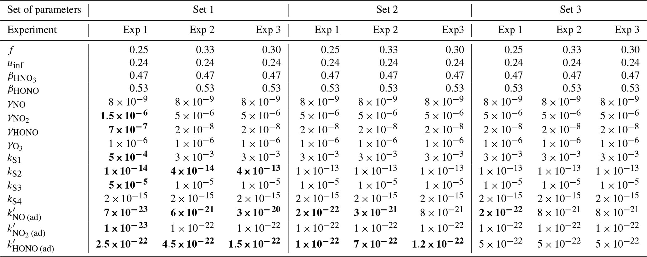
Table 6 Simulation evaluations with respect to the four modelled inorganic compounds: simulated average, relative error between simulated and measured average, root mean square error (RMSE), mean normalized gross error (MNGE), and mean normalized bias error (MNBE).

5 Sensitivity study

The purpose of this section is to investigate the relative influence of the model parameters. This section focuses on how inorganic chemistry is influenced by surface reactions. As Experiment 1 is a particular case (NO₂ injection), only Experiments 2 and 3 are considered for these tests. When a parameter is varied, the simulated results are presented for one experiment only, as the conclusions are identical for both experiments. Each tuneable parameter is investigated independently. The parameters that are not varied are given the same values as the optimized parameters (Set 1) listed in Table 5.

The initial concentrations of the gas-phase species are determined using the procedure described in Sect. 3.3 and are summarized in Table 4. The sorbed species NO_(ad), NO_2(ad), HONO_(ad) and HNO_3(ad) do not undergo the same processes as the gas-phase species. Their evolution is driven by chemical reactivity only. Since box exchange is disabled for these species, these species' profiles in the shaded and sunlit volumes are distinct, as shown by the figures presented in this section. At the start of the simulations, the concentrations of these species rapidly converge to the values determined by surface chemistry. The sorbed species initial concentrations are thus easy to set after running a couple of simulations. For a given experiment, the initial concentrations remain unchanged whatever the parameter investigated.

5.1 Filtration factor and velocity of air

Indoor chemistry is influenced by the filtration factor and the velocity of air, which are parameters characteristic of the environment. The filtration factor controls the input flux of outdoor pollutants, while the velocity of air governs deposition. This section assesses to what extent these parameters affect the overall inorganic concentrations.

5.1.1 Velocity of air

The gas-phase and adsorbed inorganic compounds simulated with a velocity of air u_inf ranging from 0.06 to 0.30 m s⁻¹ are presented in Fig. 10. This range of variations corresponds to the range of expected values described in Sect. 3.2. The modelled NO₂ and O₃ concentrations decrease with increasing u_inf, while the modelled NO and HONO concentrations increase with increasing u_inf. These opposite behaviours derive from the type of source and processes contributing the most to these species concentrations. It can be easily inferred from Eqs. (16–20) that the larger u_inf is, the larger the deposition on surfaces. When u_inf is increased, the O₃ surface removal increases. As the main source of O₃ is transport from outdoors (Weschler and Shields, 1996), this loss of O₃ is not counterbalanced by another source, which results in a decrease in O₃ with increasing u_inf. In contrast, HONO is mainly produced by heterogeneous processes that are predominant indoors. The increase in u_inf enhances NO₂ deposition and thus HONO production by NO₂ hydrolysis on surfaces. Indoor NO_x concentrations are influenced by both outdoor concentrations and surface chemistry (Weschler et al., 1994). In these experiments, variations with u_inf indicate that the main NO₂ source is outdoor infiltration, whereas NO is mainly produced by heterogeneous processes. The value retained for u_inf is 0.24 m s⁻¹, considering it is large enough to achieve effective deposition and to stimulate secondary chemistry while fulfilling the criteria presented in Sect. 3.2. As this value is the result of controlled air mixing by fans, it is kept unchanged from one experiment to the other.

Figure 10 Gas-phase and adsorbed inorganic compounds simulated with different u_inf. The blue dots denote the experimental measurements (Experiment 3). The solid lines represent the concentrations in the sunlit box and the dashed lines the concentrations in the shaded box.

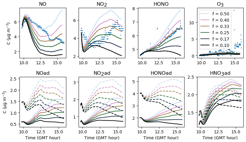
Figure 11 Gas-phase and adsorbed inorganic compounds simulated with different f. The blue dots denote the experimental measurements (Experiment 2). The solid lines represent the concentrations in the sunlit box and the dashed lines the concentrations in the shaded box.

5.1.2 Filtration factor

Contrary to u_inf, increasing f leads to an increase not only in NO₂ and O₃ but also in NO and HONO (see Fig. 11). It must be stressed that increasing f increases the intake of outdoor pollutants such as O₃, NO and NO₂, but not the losses caused by ventilation. These derive from the air exchange rate, which remains unchanged. In turn, the increased NO₂ concentration fosters the secondary production of HONO and NO. For these experiments, an average value of 0.30 appears appropriate to match the overall amount of NO_x and by extension the amount of HONO. As mentioned in Sect. 4, differences between experiments can be caused by variations in outdoor wind conditions.

5.2 NO₂ heterogeneous hydrolysis: NO_2 (ad) → 0.5 HNO_3(ad)+0.5 HONO_(ad)

The influence of NO₂ heterogeneous hydrolysis is now investigated by varying its stoichiometry and kinetic rate.

5.2.1 Stoichiometry

As introduced in Sect. 3.2, the stoichiometry of the NO₂ hydrolysis reaction can be considered somewhat uncertain. Figure 12 presents the evolution of the inorganic concentrations with different yields ${\mathit{\beta }}_{{\mathrm{HNO}}_{\mathrm{3}}}$ and β_HONO. Because HONO concentrations are underestimated when ${\mathit{\beta }}_{{\mathrm{HNO}}_{\mathrm{3}}}={\mathit{\beta }}_{\mathrm{HONO}}=\mathrm{0.5}$, the ratio ${\mathit{\beta }}_{{\mathrm{HNO}}_{\mathrm{3}}}/{\mathit{\beta }}_{\mathrm{HONO}}$ is kept <1 so that HONO_(ad) is always produced more than HNO_3(ad). When ${\mathit{\beta }}_{{\mathrm{HNO}}_{\mathrm{3}}}/{\mathit{\beta }}_{\mathrm{HONO}}$ tends to 1, the production of HONO_(ad) and HNO_3(ad) by NO₂ hydrolysis becomes balanced, which favours NO production by Reaction (S₂). NO can be converted into NO₂ by reacting with HO₂, which increases the NO₂ concentration. As less HONO_(ad) is available for desorption, less gas-phase HONO is released. Conversely, when the ratio ${\mathit{\beta }}_{{\mathrm{HNO}}_{\mathrm{3}}}/{\mathit{\beta }}_{\mathrm{HONO}}$ is decreased, the enhanced HONO_(ad) production fosters HONO desorption, leading to higher HONO and lower NO_x gas-phase concentrations. It is noteworthy that very small variations in ${\mathit{\beta }}_{{\mathrm{HNO}}_{\mathrm{3}}}/{\mathit{\beta }}_{\mathrm{HONO}}$ generate significant variations in NO_x and particularly HONO. Note that O₃ is mainly controlled by transport from outdoors and is thus not affected by these parameters. The values ${\mathit{\beta }}_{{\mathrm{HNO}}_{\mathrm{3}}}=\mathrm{0.47}$ and β_HONO=0.53 are matched to a consistent HONO production without differing too much from the classical stoichiometry assumed for this reaction. They are kept unchanged from one experiment to the other.

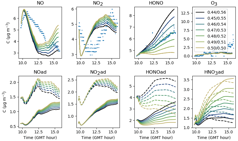
Figure 12 Gas-phase and adsorbed inorganic compounds simulated for different ${\mathit{\beta }}_{{\mathrm{HNO}}_{\mathrm{3}}}/{\mathit{\beta }}_{\mathrm{HONO}}$, with ${\mathit{\beta }}_{{\mathrm{HNO}}_{\mathrm{3}}}/{\mathit{\beta }}_{\mathrm{HONO}}<\mathrm{1}$. The blue dots denote the experimental measurements (Experiment 2). The solid lines represent the concentrations in the sunlit box and the dashed lines the concentrations in the shaded box.

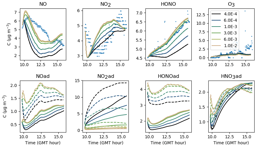
Figure 13 Gas-phase and adsorbed inorganic compounds simulated for different k_S1. The blue dots denote the experimental measurements (Experiment 2). The solid lines represent the concentrations in the sunlit box and the dashed lines the concentrations in the shaded box.

5.2.2 Surface NO₂ conversion

NO₂ is adsorbed on surfaces at a rate that is determined by the transport velocity towards surfaces and by the NO₂ uptake of surfaces. Once NO₂ is adsorbed, it is converted in the presence of water to form HONO and HNO₃ at a kinetic rate k_S1 that is highly uncertain. The larger k_S1 is, the more rapid the conversion and the larger the HONO production. The same holds for NO that is produced by the secondary reaction of HONO_(ad) with HNO_3(ad). In turn, the NO increase enhances NO₂ by homogeneous reactivity, thus providing new NO₂ available for adsorption. However, Fig. 13 shows that HONO concentrations do not vary much when k_S1 is increased above a threshold value of 0.003 s⁻¹. As k_S1 is increased above this value, the NO_2(ad) concentration tends to zero. When k_S1 is decreased, the NO_2(ad) hydrolysis is slowed down, which decreases the HONO_(ad) reservoir and thus curbs NO_y (NO_x + HONO) heterogeneous production. The sensitivity of this parameter is large. The threshold value k_S1=0.003 s⁻¹ is retained, as it maximizes the NO_2(ad) conversion.

5.3 NO secondary formation

According to Sect. 5.1.1, NO is mainly produced by secondary chemistry in these experiments. In this section, the importance of two reactions forming NO_(ad) is studied.

5.3.1 HONO_(ad) + HNO_3(ad)→2 NO_(ad)

First, NO_(ad) can be produced by the reaction of HONO_(ad) with HNO_3(ad) at a kinetic rate k_S2. Figure 14 shows that increasing k_S2 enhances the formation of NO_(ad) and thus its release to the gas phase. As less HONO_(ad) is available, the gas-phase HONO concentration is lowered. In contrast, if k_S2 is lowered, the reaction of HONO_(ad) with HNO_3(ad) becomes slower than the desorption of HONO_(ad), and most HONO_(ad) is released in the gas phase. In turn, the NO_(ad) production becomes too low to maintain an NO release allowing it to reach the measured concentrations. These results indicate that there is competition between the desorption of HONO_(ad) and the reaction of HONO_(ad) with HNO_3(ad) to consume HONO_(ad). When calibrating k_S2 and $k_{\mathrm{HONO}\left(\mathrm{ad}\right)}^{\prime }$, a balance between these two reactions must be found to obtain consistent concentration profiles for both HONO and NO. Similarly to k_S1, the parameter k_S2 seems to be a very sensitive one, as it significantly affects NO, HONO and also NO₂ through NO. The value $k_{\mathrm{S}\mathrm{2}}={\mathrm{10}}^{-\mathrm{13}}$ s⁻¹ retained for the reference simulations is a compromise between the optimized values calibrated for each experiment.

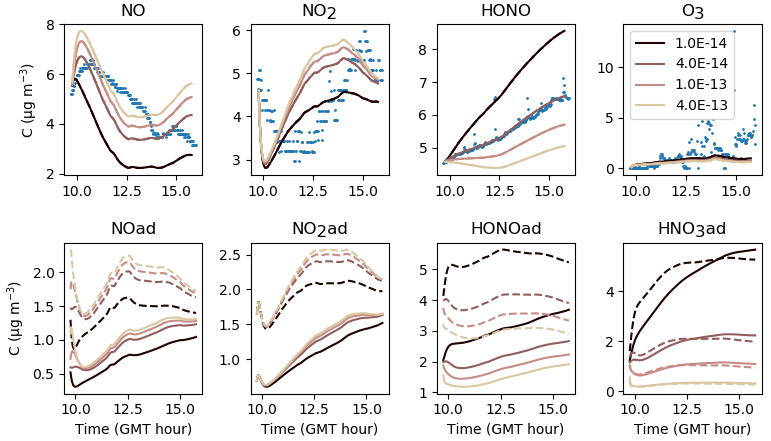
Figure 14 Gas-phase and adsorbed inorganic compounds simulated for different k_S2. The blue dots denote the experimental measurements (Experiment 2). The solid lines represent the concentrations in the sunlit box and the dashed lines the concentrations in the shaded box.

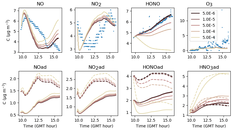
Figure 15 Gas-phase and adsorbed inorganic compounds simulated for different k_S3. The blue dots denote the experimental measurements (Experiment 2). The solid lines represent the concentrations in the sunlit box and the dashed lines the concentrations in the shaded box.

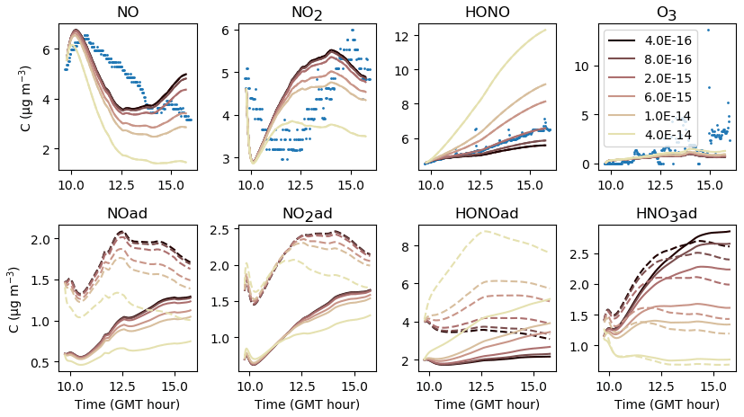
Figure 16 Gas-phase and adsorbed inorganic compounds simulated for different k_S4. The blue dots denote the experimental measurements (Experiment 2). The solid lines represent the concentrations in the sunlit box and the dashed lines the concentrations in the shaded box.

5.3.2 HONO_(ad)→0.5 NO_(ad)+0.5 NO_2(ad)

Another NO_(ad) formation pathway is the auto-ionization of HONO_(ad). The larger the kinetic constant k_S3 of this reaction is, the larger the HONO_(ad) conversion into NO_(ad) and NO_2(ad) and the lower the HONO_(ad) reservoir available for desorption. However, contrary to Reaction (S₂), the auto-ionization of HONO_(ad) does not compete with the desorption of HONO_(ad). It can be observed in Fig. 15 that when $k_{\mathrm{S}\mathrm{3}}<{\mathrm{10}}^{-\mathrm{5}}$, the effect of this reaction vanishes, indicating that the HONO concentrations are only determined by k_S2 and $k_{\mathrm{HONO}\left(\mathrm{ad}\right)}^{\prime }$: as discussed in the previous subsection, decreasing k_S2 with $k_{\mathrm{S}\mathrm{3}}={\mathrm{10}}^{-\mathrm{5}}$ enhances the release of HONO and cuts off the production of NO_(ad), showing that Reaction (S₂) and desorption weigh in on the depletion of HONO_(ad) at an equal level. If k_S3 is raised above that value, the gas-phase NO_x concentrations increase, but it becomes more difficult to lift HONO up to the concentrations measured experimentally, indicating that k_S3 should not be increased too much when calibrating the model kinetic constants. Reaction (S₃) should be kept slow compared with the desorption of HONO_(ad), which is achieved using $k_{\mathrm{S}\mathrm{3}}={\mathrm{10}}^{-\mathrm{5}}$ s⁻¹ in this work.

5.4 NO₂ regeneration: NO_(ad) + HNO_3(ad) → NO_2 (ad) + HONO_(ad)

As discussed in the Introduction, NO_2(ad) and HONO_(ad) can be regenerated through the reaction of NO_(ad) with HNO_3(ad). Figure 16 shows that the larger the kinetic constant k_S4 of this reaction is, the lower the NO and NO₂ concentrations, but the larger the HONO concentration. Increasing k_S4 promotes the consumption of NO_(ad), thus curbing the release of NO to the gas phase. The production of HONO_(ad) is enhanced, which in turn stimulates the HONO release. The production of NO_2(ad) is also enhanced by Reaction (S₄), which should increase the NO_2(ad) reservoir. However, Reaction (S₁) competes with desorption in the depletion of NO_2(ad). As Reaction (S₁) reduces the surplus of NO_2(ad) produced by Reaction (S₄), there is no increase in the NO_2(ad) reservoir. The release of NO₂ is not enhanced, and the gas-phase NO₂ concentration equilibrates with the decreased NO concentration. In turn, increasing k_S4 lowers the NO₂ concentration, whereas it raises the HONO concentration.

When k_S4 is decreased below 10⁻¹⁵, the effect of this reaction on the inorganic concentrations vanishes, showing that, similar to Reaction (S₃), Reaction (S₄) does not compete with another reaction, contrary to Reactions (S₁) and (S₂). Increasing k_S4 increases the HONO concentration but lessens the NO_x level at the same time, which is unfavourable beyond a certain threshold. This suggests that the kinetic constant k_S4 should remain low enough to maintain Reaction (S₄) upstage as Reaction (S₃). In these simulations, the value $k_{\mathrm{S}\mathrm{4}}=\mathrm{2}\times {\mathrm{10}}^{-\mathrm{15}}$ allows HONO production to be supported while meeting this requirement.

5.5 Desorption constants and uptake values

The desorption constants and uptake coefficients drive the exchanges between the adsorbed and the gas phases. They are now examined.

5.5.1 Nitrogen dioxide

The uptake coefficient ${\mathit{\gamma }}_{{\mathrm{NO}}_{\mathrm{2}}}$ is the only parameter characteristic of the heterogeneous chemistry of inorganic compounds that was determined experimentally for the paint boards. This parameter is not modified in Experiments 2 and 3 in which the paint boards were used. Here, the sorption dynamics of NO₂ are only modified through the desorption constant $k_{{\mathrm{NO}}_{\mathrm{2}}\left(\mathrm{ad}\right)}^{\prime }$. It can be inferred from Fig. 17 that the NO₂ concentration is not very sensitive to $k_{{\mathrm{NO}}_{\mathrm{2}}\left(\mathrm{ad}\right)}^{\prime }$, as the latter must be varied over several orders of magnitude to observe significant changes in NO₂ concentrations, likely because the main source of NO₂ is transport from outdoors and not secondary chemistry. Increasing $k_{{\mathrm{NO}}_{\mathrm{2}}\left(\mathrm{ad}\right)}^{\prime }$ decreases the NO_2(ad) reservoir. As less NO_2(ad) is available, less HONO_(ad) is produced by Reaction (S₁), thus resulting in a decreased release of HONO to the gas phase. To maintain sufficient NO₂ adsorption and a large enough HONO concentration, the parameter $k_{{\mathrm{NO}}_{\mathrm{2}}\left(\mathrm{ad}\right)}^{\prime }$ should be kept low. It is set to $k_{{\mathrm{NO}}_{\mathrm{2}}\left(\mathrm{ad}\right)}^{\prime }={\mathrm{10}}^{-\mathrm{22}}$ s⁻¹ molec.⁻¹ in the reference simulations.

Figure 17 Gas-phase and adsorbed inorganic compounds simulated for different $k_{{\mathrm{NO}}_{\mathrm{2}}\left(\mathrm{ad}\right)}^{\prime }$. The blue dots denote the experimental measurements (Experiment 3). The solid lines represent the concentrations in the sunlit box and the dashed lines the concentrations in the shaded box.

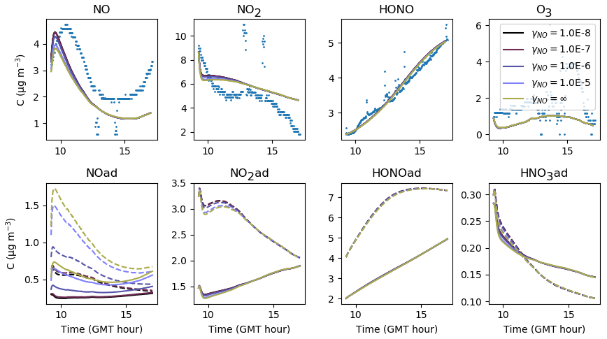
Figure 18 Gas-phase and adsorbed inorganic compounds simulated for different γ_NO. The blue dots denote the experimental measurements (Experiment 3). The solid lines represent the concentrations in the sunlit box and the dashed lines the concentrations in the shaded box.

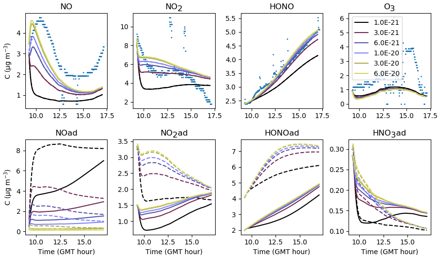
Figure 19 Gas-phase and adsorbed inorganic compounds simulated for different $k_{\mathrm{NO}\left(\mathrm{ad}\right)}^{\prime }$. The blue dots denote the experimental measurements (Experiment 3). The solid lines represent the concentrations in the sunlit box and the dashed lines the concentrations in the shaded box.

5.5.2 Nitric oxide

To date, all box models (Sarwar et al., 2002; Carslaw, 2007; Courtey et al., 2009; Mendez et al., 2015) assume a zero deposition velocity for NO after the values reported by Nazaroff and Cass (1986). A zero deposition velocity corresponds to an uptake coefficient close to zero, thus preventing the molecules from colliding with surfaces and becoming adsorbed.

Figure 18 investigates the sensitivity of inorganic concentrations to γ_NO, which is varied between ${\mathit{\gamma }}_{\mathrm{NO}}={\mathrm{10}}^{-\mathrm{8}}$ and the maximum value γ_NO=∞. The coefficient γ_NO=∞ is obtained by assuming that all collisions are efficient, i.e. $k_{\mathrm{DEP},i}^j=k_{\mathrm{tran},i}^j$. When γ_NO=∞, the NO deposition is only limited by transport to the surface. Apart from the beginning of the simulations, no significant variation in the NO concentration is observed between the extreme values investigated, showing that in this experiment, deposition has a negligible contribution to the gas-phase NO concentration. The first part of the simulated profile can be improved by about 10 % using the lowest γ_NO value.

The concentration variations with desorption constant $k_{\mathrm{NO}\left(\mathrm{ad}\right)}^{\prime }$ are presented in Fig. 19. When $k_{\mathrm{NO}\left(\mathrm{ad}\right)}^{\prime }$ is increased, NO_(ad) evaporates towards the gas phase. In contrast, when $k_{\mathrm{NO}\left(\mathrm{ad}\right)}^{\prime }$ is decreased, the release of NO is less efficient and the NO concentration decreases, leading to a decrease in the NO₂ concentration. Then, since less NO₂ is available on surfaces for hydrolysis, less HONO is produced. As a result, decreasing $k_{\mathrm{NO}\left(\mathrm{ad}\right)}^{\prime }$ too much decreases the three NO_y compound concentrations in the gas phase.

In turn, the parameters γ_NO and $k_{\mathrm{NO}\left(\mathrm{ad}\right)}^{\prime }$ should be fixed to maintain NO in the gas-phase form preferentially, which corroborates the use of a very low deposition velocity, as reported in the literature. In this paper, an uptake coefficient ${\mathit{\gamma }}_{\mathrm{NO}}=\mathrm{8}\times {\mathrm{10}}^{-\mathrm{9}}$ is chosen for all simulations. The desorption constant $k_{\mathrm{NO}\left(\mathrm{ad}\right)}^{\prime }$ is set to $\mathrm{8}\times {\mathrm{10}}^{-\mathrm{21}}$ s⁻¹ molec.⁻¹ for Experiments 2 and 3, while a lower value $\mathrm{2}\times {\mathrm{10}}^{-\mathrm{22}}$ s⁻¹ molec.⁻¹ appears to be required to simulate Experiment 1.

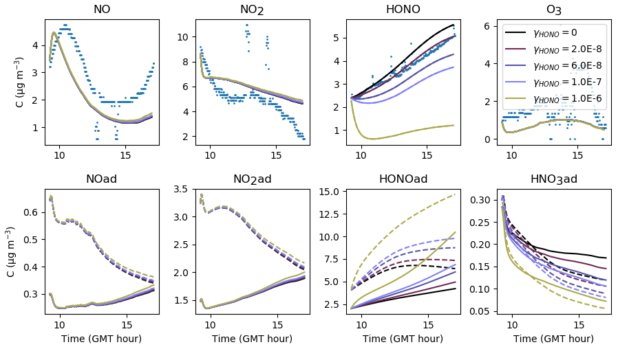
Figure 20 Gas-phase and adsorbed inorganic compounds simulated for different γ_HONO. The blue dots denote the experimental measurements (Experiment 3). The solid lines represent the concentrations in the sunlit box and the dashed lines the concentrations in the shaded box.

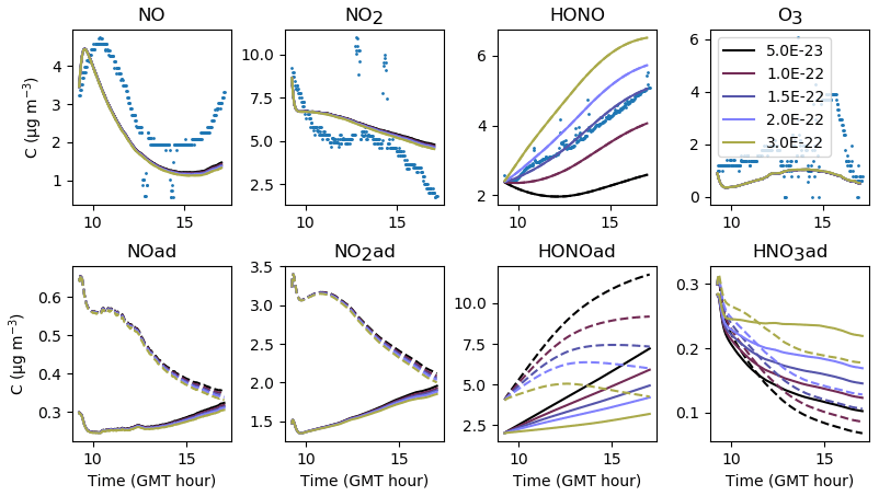
Figure 21 Gas-phase and adsorbed inorganic compounds simulated for different $k_{\mathrm{HONO}\left(\mathrm{ad}\right)}^{\prime }$. The blue dots denote the experimental measurements (Experiment 3). The solid lines represent the concentrations in the sunlit box and the dashed lines the concentrations in the shaded box.

Figure 22 Gas-phase and adsorbed inorganic compounds simulated for different ${\mathit{\gamma }}_{{\mathrm{O}}_{\mathrm{3}}}$. The blue dots denote the experimental measurements (Experiment 3). The solid lines represent the concentrations in the sunlit box and the dashed lines the concentrations in the shaded box.

5.5.3 Nitrous acid

The adsorption–desorption dynamics of HONO are investigated by varying the uptake coefficient γ_HONO (Fig. 20) and the desorption constant $k_{\mathrm{HONO}\left(\mathrm{ad}\right)}^{\prime }$ (Fig. 21). Contrary to NO, small variations in the uptake coefficient and desorption constant cause the HONO concentration to vary greatly. HONO is not brought by transport from the outdoors and is only produced by secondary chemistry, which justifies the critical importance of these parameters in controlling the transfers between the homogeneous gas phase and surfaces. Increasing γ_HONO leads to increasing the HONO_(ad) reservoir and therefore to decreasing the gas-phase HONO. When γ_HONO tends to zero, the gas-phase HONO concentration is determined by the desorption constant $k_{\mathrm{HONO}\left(\mathrm{ad}\right)}^{\prime }$ only. As the HONO concentration is sensitive to both γ_HONO and $k_{\mathrm{HONO}\left(\mathrm{ad}\right)}^{\prime }$, a balance between these parameters must be found. An increase in γ_HONO can compensate for an increase in $k_{\mathrm{HONO}\left(\mathrm{ad}\right)}^{\prime }$, and, reciprocally, a decrease in γ_HONO must be associated with a decrease in $k_{\mathrm{HONO}\left(\mathrm{ad}\right)}^{\prime }$. Several choices (large γ_HONO and $k_{\mathrm{HONO}\left(\mathrm{ad}\right)}^{\prime }$ vs. low γ_HONO and $k_{\mathrm{HONO}\left(\mathrm{ad}\right)}^{\prime }$) can simulate the HONO concentration correctly. However, the time variations of the HONO concentration may behave differently depending on the chosen set of parameters. In this example, if both γ_HONO and $k_{\mathrm{HONO}\left(\mathrm{ad}\right)}^{\prime }$ are large, the HONO concentration tends to decrease at the end of the simulation, whereas a monotonous increase is observed in the experiment. This suggests that low values of γ_HONO and $k_{\mathrm{HONO}\left(\mathrm{ad}\right)}^{\prime }$ are better suited. The values ${\mathit{\gamma }}_{\mathrm{HONO}}=\mathrm{2}\times {\mathrm{10}}^{-\mathrm{8}}$ and $k_{\mathrm{HONO}\left(\mathrm{ad}\right)}^{\prime }=\mathrm{5}\times {\mathrm{10}}^{-\mathrm{22}}$ s⁻¹ molec.⁻¹ are retained for the reference simulations. By comparison, considering an average humidity of 45 %, the relationship between humidity and γ_HONO measured on TiO₂ surfaces, found by El Zein and Bedjanian (2012) under dark conditions, gives ${\mathit{\gamma }}_{\mathrm{HONO}}=\mathrm{1.6}\times {\mathrm{10}}^{-\mathrm{6}}$, which is a value higher than the one determined here. However, we recall that the same uptake value is used for all materials constituting the room (walls, floor and window), which complicates the analogy.

Finally, while significant variations of HONO concentrations are observed, changes in NO and NO₂ are imperceptible, thus showing the poor correlation between HONO and NO_x concentrations in these experiments with anti-UV windows.

5.5.4 Ozone

In all simulations presented above, the O₃ concentrations are not altered by any change in NO_x and HONO concentrations. This is an expected behaviour, considering that the main source of O₃ is transport from the outdoors and that its main sink is deposition. Figure 22 shows that variations in the uptake coefficient ${\mathit{\gamma }}_{{\mathrm{O}}_{\mathrm{3}}}$ modify the O₃ concentration significantly and also the NO concentration through homogeneous chemistry. When ${\mathit{\gamma }}_{{\mathrm{O}}_{\mathrm{3}}}$ tends to zero, the O₃ concentration increases up to a value very close to the experimental one, whereas the NO concentration decreases to concentrations much lower than those observed. With an uptake coefficient ${\mathit{\gamma }}_{{\mathrm{O}}_{\mathrm{3}}}={\mathrm{10}}^{-\mathrm{6}}$ and no desorption reaction for O₃, both O3 and NO are correctly modelled: although lower than the experimental record, O₃ remains within 60 % of the measured concentration, while the NO RMSE remains close to 1.

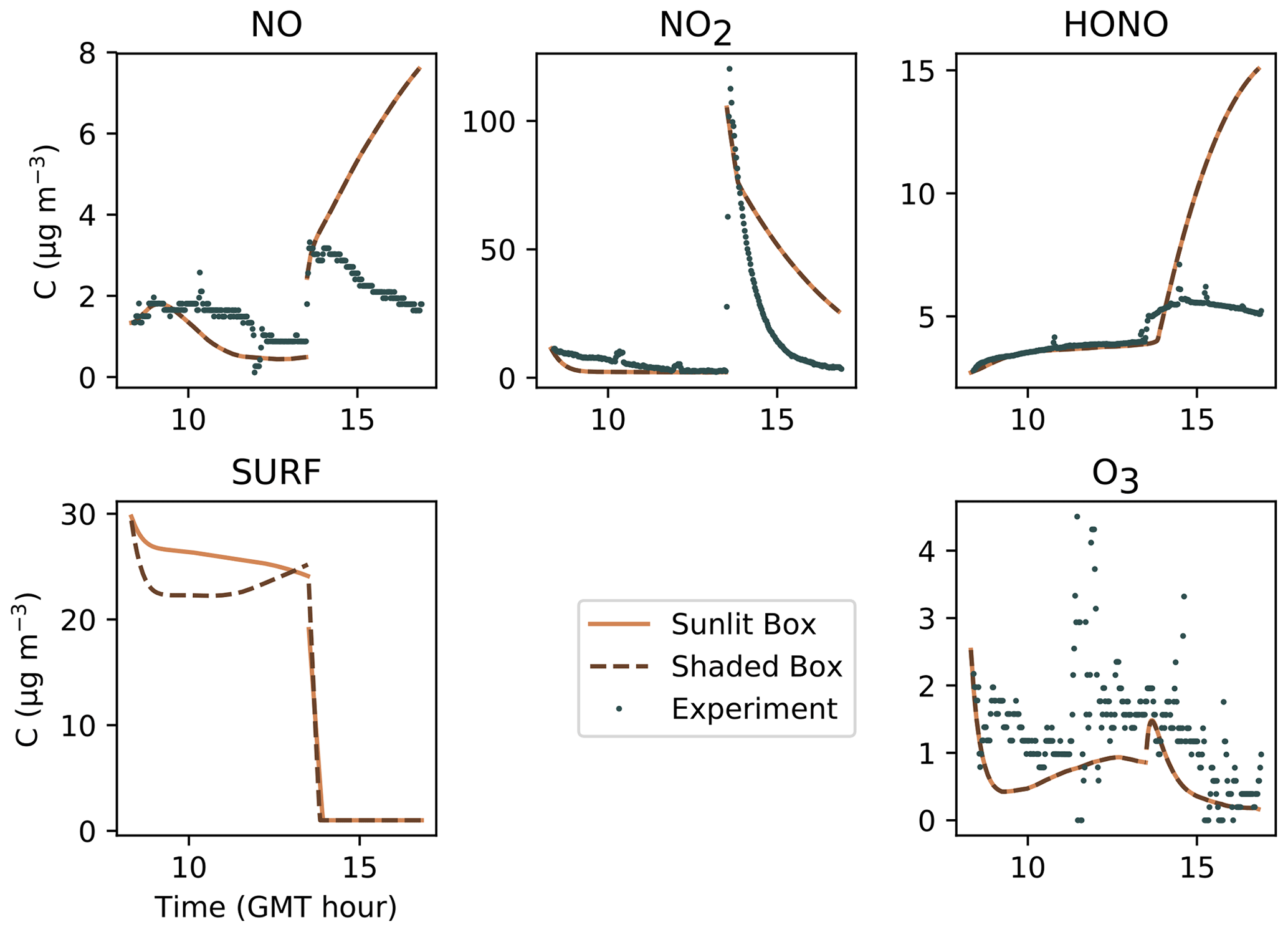
Figure 23 Implementation of a surface saturation effect using the compound SURF. The dots denote the experimental records, the solid lines denote the concentrations simulated in the sunlit box, and the dashed lines denote the concentrations in the shaded box.

6 Modelling high NO₂ concentrations: focus on Experiment 1

When analysing the optimized simulations, it can be noticed that the parameters fitting Experiments 2 and 3 are similar but can significantly differ from some of those fitting Experiment 1, especially the ones controlling the adsorption–desorption of the NO_y compounds. The difficulty in simulating Experiment 1 (Fig. 7) lies in handling the fast transition from a moderate NO₂ concentration to a very high one. To prevent the HONO and NO secondary production from rocketing after the NO₂ injection, $k_{\mathrm{NO}\left(\mathrm{ad}\right)}^{\prime }$ was decreased and γ_HONO was increased to limit the NO and HONO releases. To preserve satisfying NO and HONO levels before the injection, the initial concentrations of NO_(ad) and HONO_(ad) were increased in order to counterbalance the weaker release of these species.

In spite of the above, changing the model parameters could not completely mitigate the NO and HONO breakouts caused by the massive NO₂ supply. Previously, the modelling of the HONO production in high NO₂ conditions, i.e. NO₂ concentrations exceeding 25 ppb, was already pointed out by Mendez et al. (2017) as a challenging issue. As in this study, the experimental HONO step-up caused by the NO₂ injection was moderate, which the existing model failed to replicate by overestimating the HONO increase. Mendez et al. (2017) proposed coping with this by introducing a compound, SURF, representing the number of sites available for NO₂, thus limiting the amount of NO_2(ad) for surface hydrolysis.

In this paper, a similar solution is implemented by extending the definition of SURF to all surface compounds introduced in this model. Here, SURF represents the number of sites available for NO, HONO, NO₂ and HNO₃. SURF is incorporated in the adsorption–desorption reactions but only modifies the kinetics of these reactions when its “concentration” is less than unity. In other words, as long as many surface sites are available, the sorption dynamics behave as usual, but as soon as the surface approaches saturation, the kinetics of the adsorption reactions are increased by 1 order, in addition to being slowed down by the SURF “concentration” being less than unity.

The resulting profiles are presented in Fig. 23 using the same parameters as the optimized simulation. An important difference with Mendez et al. (2017) is that the NO, NO₂ and O₃ concentrations are not fixed to their measured values. In this test, the NO₂ injection causes the three NO_y compounds to increase. The magnitude of this increase is determined by the initial value of the SURF concentration. When this value is very large, the concentration profiles converge to the optimized simulation (Fig. 7). Conversely, when the initial SURF concentration is decreased, the sorption of NO₂ and related species is reduced, which generates an excess of gas-phase NO_y.

From Fig. 23, we may conclude that the parameterization of desorption needs improvement or that the contribution of NO₂ to the secondary formation of HONO and NO is overestimated. These results agree with the work of Collins et al. (2018), who performed indoor time-resolved measurements of HONO and NO₂ under both positive and negative perturbations. Their measurements indicated a weak correlation between the concentrations of both species. Similar behaviour was observed during the SURFin campaign (Alvarez et al., 2013), during which the HONO concentration increased rapidly after ventilation periods and remained in a near-steady state despite NO₂ variations. The SURF compound introduced by Mendez et al. (2017) to model these data made it possible to decrease the coupling between the two species. However, the modelled HONO concentration still retained more sensitivity to NO₂ than what the measurements indicated. It appears from Fig. 23 that extending the definition of SURF to all sorbed compounds introduced in this model does not improve the problem.

7 Discussion

Considering the number of parameters involved in this model, a given simulation result is likely reachable by different parameter combinations. Additionally, some parameters that could replicate the records presented in this study are typical of the room where the experiments took place and would be hardly transferable to other indoor environments. These are the filtration factor, velocity of the air, desorption constants and uptake coefficients. Although these parameters are basically environmentally dependent and non-unique, several conclusions can be drawn from these tests regarding general principles of IAQ modelling.

The air-mixing velocity introduced as in Mendez et al. (2017) appears to be a critical parameter for the four main species leading the inorganic chemistry. The building filtration factor, generally taken as unity, is also a determining factor. This parameter should not be confused with the ventilation rate (k_AER) that encompasses leaks to both the outside and to the rest of the building. The building filtration factor controls the fraction of air influx coming from outside the building. In these experiments, its value is far from unity, thus featuring low infiltration. Using a value of unity would have led to overestimating the intake of outdoor pollutants, thus mitigating the importance of heterogeneous phenomena.

The surface hydrolysis of NO₂ produces sorbed HONO and HNO₃ that further react to produce sorbed NO. The kinetics of this reaction are determined by its kinetic rate k_S1 and also by the NO₂ adsorption–desorption reactions that control the variations of the NO_2(ad) reservoir. The NO_2(ad) concentration variations largely influence the variations of the other sorbed species concentrations through Reaction (S₁), which could be considered the cornerstone of indoor heterogeneous chemistry in this model. A very small adjustment in the stoichiometry of Reaction (S₁) allows a significant increase in the HONO secondary production in all experiments.

The NO secondary production mainly derives from Reaction (S₂), which competes with the HONO desorption. The kinetic rates of these reactions can be influenced by the nature of the surface materials. The release kinetics of these species flow from their sorbed concentrations, which likely depend on a variety of parameters. This environmental dependence could explain why the yields of HONO and NO reported in the literature can vary a lot from one study to another (Finlayson-Pitts et al., 2003). Reactions (S₃) and (S₄) can influence the NO_y concentration time variations, but their impacts seem less predominant.

Regarding the sorption dynamics, HONO is extremely sensitive to the values of its uptake coefficient and desorption constant, since it is almost entirely produced by heterogeneous chemistry. Obviously, these parameters have antagonist effects that can neutralize each other. The proper calibration of these parameters can be oriented by the shape of the sorbed species profile with respect to the gas-phase experimental profile. Contrary to HONO, the NO concentration does not seem to be affected by the uptake coefficient γ_NO. Similarly to the OH radical, NO is likely too reactive to be affected by deposition. When deposition has a negligible contribution compared with homogeneous reactivity, the influence of the species uptake coefficient on the gas-phase concentration can be considered to be null, whatever its genuine value may be. In this case, the uptake coefficient can be set to zero as an apparent uptake value.

The simulations presented in Sect. 4 show that the desorption constants are the parameters that are the most difficult to set, especially for NO and HONO. The problem is less striking for NO₂ since the main source of NO₂ is transport from the outdoors in these experiments. By using a common value of $k_{\mathrm{HONO}\left(\mathrm{ad}\right)}^{\prime }$ for the three experiments (reference simulations), the simulated HONO concentrations show an overestimation of 95 % and 78 % for Experiments 1 and 3. Using the same $k_{\mathrm{NO}\left(\mathrm{ad}\right)}^{\prime }$ in Experiments 2 and 3, the simulated NO concentrations remain as similar to the measured concentrations as using the optimized parameters. However, it is impossible to use the same value in Experiment 1 without making the NO concentration increase well above the measured values.

Small variations in uptake coefficients and desorption constants can be supported by differences in wall covering between experiments. In the first experiment, walls were naked, whereas in subsequent experiments, walls were covered by boards freshly coated with a paint made of the same organic matrix. According to Finlayson-Pitts et al. (2003), the composition of the surface film of water can play an important role in determining the yields of NO and HONO, but the nature of the underlying material should not influence this chemistry unless it is sufficiently reactive to modify the composition of the surface film. The surface topology can also influence the material adsorption capacity: experiments conducted by Wainman et al. (2001) to study the influence of the surface nature on NO₂ hydrolysis showed that HONO concentrations were significantly enhanced when synthetic carpet was used instead of Teflon surfaces. They suggested that this was caused by the greater surface quantity provided by the carpet fibres, allowing more room for the reaction to occur. In this study, it could be argued that differences in roughness between the walls and paint boards, combined with differences in uptake values, may account for variations of surface sorption capacity between the first and following experiments. However, these elements are not sufficient to support a difference in $k_{\mathrm{NO}\left(\mathrm{ad}\right)}^{\prime }$ of almost 3 orders of magnitude (see Set 1 in Table 5).

In light of this, it can be inferred that a more sophisticated parameterization of the desorption reactions may be required to improve this model. Rather than competitive adsorption–desorption kinetics, the adsorption–desorption phenomenon may be represented by an equilibrium approach, which depends on the mass ratio of adsorbed to gas phase. Such improvement may also alleviate the problems observed after the NO₂ injection during Experiment 1. Similar to Mendez et al. (2017), we observe that the measured increase in HONO after the NO₂ injection is moderate, and similar to the models tested by Mendez et al. (2017), the H²I model overestimates this increase in HONO concentration. Collins et al. (2018) succeeded in simulating gas-phase HONO at a high NO₂ level using persistent source and sink processes with only a small contribution from NO₂ uptake. To explain the poor correlation between the two species concentrations, Collins et al. (2018) suggested that gas-phase HONO could be in equilibrium with a precursor reservoir of nitrite and/or HONO dissolved in surface films or sorbed on surfaces. Thanks to the introduction of the compound HONO_(ad), the current model includes this type of reservoir. Indeed, the HONO produced by Reaction (S₁) first remains adsorbed before being released to the gas phase. However, even considering an intermediate compound HONO_(ad), the connection between NO₂ and HONO remains too strong. A different type of desorption model based on equilibrium rather than competition for surface sites may decrease this coupling. In addition, introducing another compound interacting with HONO_(ad), such as nitrite, should further decrease the influence of Reaction (S₁) on the HONO_(ad) concentration and thus further attenuate the dependence of the gas-phase HONO on NO₂.

8 Conclusions

In this paper, a new numerical model combining homogeneous and heterogeneous chemistry is implemented and proved able to simulate the concentrations of inorganic compounds. For the first time, O₃, HONO and NO_x species are simulated all at once and compared with the experimental records acquired in a real room. The specificity of this model is to incorporate secondary reactions that were highlighted by laboratory studies but that are still absent from IAQ models. It is also one of the first models to consider the variations of direct and indirect light throughout the day. This feature is of particular importance in studying the impact of photolytic processes on indoor chemistry. After developing and testing the model in the absence of these processes in the present work, it can now be used to simulate data obtained with UV-transparent windows that allow photochemistry to occur.

The comparison between the simulation results and experimental data allowed the tuning of the model parameters, which led to several conclusions: (i) the building filtration factor and velocity of air mixing are important parameters that should receive more attention; (ii) for the considered simulation duration (a third of one day on average), the proper assessment of the initial concentrations is critical; (iii) whereas deposition and surface reactivity are treated together by current models, the distinction between sorption and surface reactions appears to be essential. This distinction is based on the introduction of sorbed species that also have the possibility to desorb. To better constrain these sorption–desorption processes, there is a need for surface material characterization, especially for measurements of O₃, NO₂ and HONO uptake coefficients and for NO, NO₂ and HONO desorption constants in various conditions of temperature, humidity and irradiation. (iv) The success of this model in simulating inorganic species largely arises from better consideration of surface chemistry. Whereas Reactions (S₃) and (S₄) could be considered to be of secondary importance, Reaction (S₂) appears to be as important as Reaction (S₁), which is currently the only surface reaction taken into account in IAQ models. Reaction (S₂) may account for unexplained variations in NO vs. HONO production ratios and should clearly be integrated. Finally, the implementation of a surface saturation effect highlights the need for a more complex parameterization of desorption. In the future, further investigations using an equilibrium-type approach that depends on the mass ratio of adsorbed to gas phase may bring key improvements.

Appendix A: List of symbols

Symbol	Description	Unit
αi	Tuneable variable allowing control of the desorption of species i	kg bar−1 mol−1
${\mathit{\beta }}_{\mathrm{HONO}/{\mathrm{HNO}}_{\mathrm{3}}}$	Stoichiometric coefficients of the NO2 heterogeneous hydrolysis	–
$C_i^j$	Concentration of species i in the box j	µg m−3
$C_i^{\mathrm{Out}}$	Outdoor concentration of species i	µg m−3
Di	Diffusion coefficient of species i	m2 s−1
η	Air dynamic viscosity	kg m−1 s−1
f	Outdoor-to-indoor filtration factor	–
G	Marker referring to the shaded box	–
γi	Uptake coefficient of species i	–
H	Relative humidity	–
I	Light intensity	W m−2
Ji	Photolysis constant of species i	photons cm−2 s−1
ki,(ad)	Desorption constant of species i	s−1 molec.−1
kH,i	Henry's law constant of species i	bar mol kg−1
kAER	Air exchange rate between the room and outside the room	s−1
$k_{\mathrm{BOX}}^j$	Air exchange rate between the boxes	s−1
$k_{\mathrm{DEP},i}^j$	Deposition rate of species i in box j	s−1
$k_{\mathrm{react},i}^j$	Surface adhesion rate of species i in box j	s−1
$k_{\mathrm{tran},i}^j$	Transport-limited deposition rate of species i in box j	s−1
kS	Kinetic rate of Reaction (S)	s−1
κi	Cross section of species i	–
L	Marker referring to the sunlit box	–
l	Characteristic length of the room	m
λ	Light wavelength	nm
Mi	Molar mass of species i	g mol−1
$m_i^j$	Mass of species i in box j	µg
$m_i^{\mathrm{Out},j}$	Outdoor mass of species i introduced in box j	µg
μ,σ	Gaussian function parameters	h, h
N	NO2 concentration (ppb)	–
$n_{{\mathrm{H}}_{\mathrm{2}}\mathrm{O}}$	Number of water molecules in the room	–
ν	Air kinematic viscosity	m2 s−1
ωi	Thermal velocity of species i	m s−1
P	Ambient pressure	Pa
ϕi	Quantum yield of species i	–
Qpi	Emission rate of species i from source p	µg s−1
$R_{iq}^j$	Mass reaction rate of species i with species q in box j	µg s−1
ρ	Air volumetric mass	kg m−3
Sgas	Surface allowing gas transfer between the two boxes	m2
$S_{\mathrm{paint}}^j$	Surface of paint in the box j	m2
Sroom	Total surface of the room	m2
Sη	Sutherland's constant	K
T	Room temperature	K
Tc,i	Critical temperature of species i	K
t	Time	s
th	Hour of day (GMT)	h
θ	Zenith angle	–

Symbol	Description	Unit
U	Mean air velocity parallel to the surface	m s−1
u*	Friction velocity	m s−1
uinf	Average velocity of air in the room	m s−1
Vc,i	Critical volume of species i	cm3 mol−1
$V_{\mathrm{box}}^j$	Volume of box j	m3
Vroom	Total volume of the room	m3
vtrd,i	Transport-limited deposition velocity of species i	m s−1
y	Distance from surface	m
ζ	Actinic flux	photons cm−2 nm−1

Appendix B: Concentration initialization

This Appendix presents the figures corresponding to the initialization procedure described in Sect. 3.3. In these figures, “No init” is the simulation performed without initializing the compounds which were not detected during the campaign. “Reference” is the simulation run corresponding to the optimized simulation (see Sect. 4). The correspondence between these simulation runs and the experimental concentrations is assessed by computing the MNGE over the first 5000 s, denoted by the red dots, for NO and NO₂.

Figure B1 Concentration initialization for Experiment 1: for this experiment, proper initial concentrations are considered to be achieved when the MNGE with respect to NO reaches a minimum. The MNGE of NO₂ remains high because the parameter optimization regarding NO₂ focused on the correct modelling of the second part of the experiment (see Sect. 6, modelling high NO₂ concentrations).

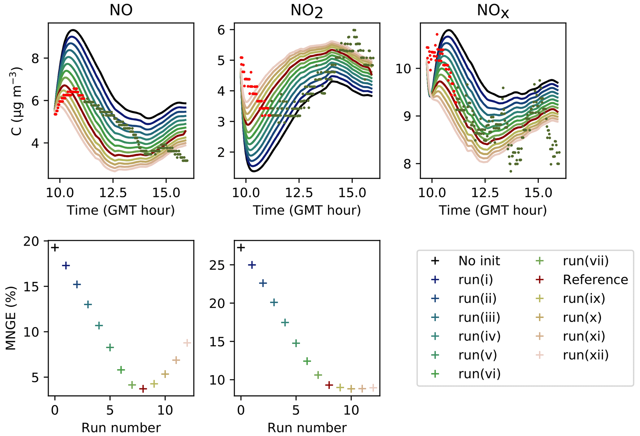
Figure B2 Concentration initialization for Experiment 2: for this experiment, proper initial concentrations are considered to be achieved when the MNGE with respect to NO reaches a minimum, while the MNGE of NO₂ reaches stabilization.

Figure B3 Concentration initialization for Experiment 3: for this experiment, proper initial concentrations are considered to be achieved when the MNGEs with respect to NO and NO₂ have converged to stable values.