Developing a common, flexible and efficient framework for weakly coupled ensemble data assimilation based on C-Coupler2.0

Data assimilation (DA) provides initial states of model runs by combining observational information and models. Ensemble-based DA methods that depend on the ensemble run of a model have been widely used. In response to the development of seamless prediction based on coupled models or even Earth system models, coupled DA is now in the mainstream of DA development. In this paper, we focus on the technical challenges in developing a coupled ensemble DA system, especially how to conveniently achieve efficient interaction between the ensemble of the coupled model and the DA methods. We first propose a new DA framework, DAFCC1 (Data Assimilation Framework based on C-Coupler2.0, version 1), for weakly coupled ensemble DA, which enables users to conveniently integrate a DA method into a model as a procedure that can be directly called by the model ensemble. DAFCC1 automatically and efficiently handles data exchanges between the model ensemble members and the DA method without global communications and does not require users to develop extra code for implementing the data exchange functionality. Based on DAFCC1, we then develop an example weakly coupled ensemble DA system by combining an ensemble DA system and a regional atmosphere–ocean–wave coupled model. This example DA system and our evaluations demonstrate the correctness of DAFCC1 in developing a weakly coupled ensemble DA system and the effectiveness in accelerating an offline DA system that uses disk files as the interfaces for the data exchange functionality.

1 Introduction

Data assimilation (DA) methods, which provide initial states of model runs by combining observational information and models, have been widely used in weather forecasting and climate prediction. The ensemble Kalman filter (EnKF; Houtekamer and Mitchell, 1998; Evensen, 2003; Lorenc, 2003a; Anderson and Collins, 2007; Whitaker, 2012) is a widely used DA method that depends on an ensemble run of members. Other DA methods such as the nudging method (Hoke and Anthes, 1976; Vidard et al., 2003), optimal interpolation (OI; Gandin, 1966), ensemble OI (EnOI; Oke et al., 2002; Evensen, 2003), three-dimensional variational analysis (3D-Var; Anderson et al., 1998; Courtier et al., 1998; Gauthier et al., 1999; Lorenc et al., 2000) and four-dimensional variational analysis (4D-Var; Courtier et al., 1994; Kalnay, 2002; Lorenc, 2003b; Rabier et al., 2007) can be technically viewed as a special case of ensemble-based methods with only one member in the ensemble when we attempt to design and develop a software framework for data assimilation. Moreover, hybrid DA methods, such as hybrid ensemble and 3D-Var (Hamill, 2000; Etherton and Bishop, 2004; Wang et al., 2008, 2013; Ma et al., 2014) and ensemble-based 4D-Var schemes (Fisher, 2003; Bishop and Hodyss, 2011; Bonavita et al., 2012, 2016; Buehner et al., 2015), also depend on the ensemble run of members from the same model.

With the rapid development of science and technology, numerical forecasting systems are evolving from only an individual component model (such as an atmospheric model) to coupled models that can achieve better predictability (Brown et al., 2012; Mulholland et al., 2015), and Earth system models are being used to develop seamless predictions that span timescales from minutes to months or even decades (Palmer et al., 2008; Hoskins, 2013). Along with the use of coupled models in numerical forecasting, common and flexible DA methods for coupled models are urgently needed (Brunet et al., 2015; Penny et al., 2017). Coupled DA technologies have already been investigated widely, and DA systems have been constructed (Sugiura et al., 2008; Fujii et al., 2009, 2011; Saha et al., 2010, 2014; Sakov et al., 2012; Yang et al., 2013; Tardif et al., 2014, 2015; Lea et al., 2015; Lu et al., 2015a, b; Mochizuki et al., 2016; Laloyaux et al., 2016, 2018; Browne et al., 2019; Goodliff et al., 2019; Skachko et al., 2019) in which ensemble-based DA methods have already been applied (e.g., Zhang et al., 2005, 2007; Sluka et al., 2016).

To develop a coupled ensemble DA system, besides the scientific challenges regarding DA methods, there are also technical challenges to be addressed, such as how to achieve an ensemble run of a coupled model, how to conveniently integrate the software of a coupled model and the software of ensemble DA methods into a robust system, and how to conveniently achieve efficient interaction between the ensemble of the coupled model and the DA methods. The existing ensemble DA frameworks supporting coupled DA such as the Data Assimilation Research Testbed (DART; Anderson et al., 2009) and the Grid point Statistical Interpolation (GSI; Shao et al., 2016) combined with EnKF (H. Liu et al., 2018), employ disk files as the interfaces of data exchange between the model ensemble members and the DA methods, and iteratively switch between the run of the model ensemble and DA using software-based restart functionality that also relies on disk files. Such an implementation (called offline implementation hereafter) can guarantee software independence between the models and the DA methods, so as to achieve flexibility and convenience in software integration; however, the extra I/O accesses of disk files, as well as the extra initialization of software modules introduced by the data exchange and the restarts, are time-consuming and can be a severe performance bottleneck under finer model resolution (Heinzeller et al., 2016; Craig et al., 2017). The Parallel Data Assimilation Framework (PDAF; Nerger et al., 2005; Nerger and Hiller, 2013; Nerger et al., 2020) and the Employing Message Passing Interface for Researching Ensembles (EMPIRE; Browne and Wilson, 2015) framework have shown that MPI (Message Passing Interface)-based data exchanges between the model ensemble members and DA procedures can produce better performance for DA systems because they do not require disk files or the restart operations.

Noting that most existing couplers for Earth system modeling have already achieved flexible MPI-based data exchanges between component models in a coupled system, we design and develop a common, flexible and efficient framework for coupled ensemble data assimilation, based on the latest version of the Community Coupler (C-Coupler2.0; L. Liu et al., 2018). Considering that existing observation processing systems can introduce different observation frequencies corresponding to different component models, we take consideration of weakly coupled ensemble DA where the data from different component models are assimilated independently by separate DA methods (Zhang et al., 2005, 2007; Fujii et al., 2009, 2011; Saha et al., 2010, 2014) in this work, and further work will then target strongly coupled ensemble DA, which generally uses a cross-domain error covariance matrix to account for the impact of the same observational information on different component models cooperatively (Tardif et al., 2014, 2015; Lu et al., 2015a, b; Sluka et al., 2016).

The remainder of this paper is organized as follows. Section 2 introduces the overall design of the new DA framework named DAFCC1 (Data Assimilation Framework based on C-Coupler2.0, version 1). The implementation of DAFCC1 is described in Sect. 3. Section 4 introduces the development of an example weakly coupled ensemble DA system based on DAFCC1. Section 5 evaluates DAFCC1. Finally, Sect. 6 contains a discussion and conclusions.

2 Overall design of the new framework

The experiences gained from PDAF and EMPIRE show that a framework with an online implementation that handles the data exchanges via MPI functionalities is essential for improving the interaction between the model and the DA software. There can be different strategies for the online implementation. In EMPIRE, a DA method is compiled into a stand-alone executable running on the processes distinct from the model ensemble, and global communications with MPI_gatherv and MPI_scatterv are used for exchanging data between the model ensemble and the DA method. Such an implementation can maintain the independence between the DA software and the model but is inefficient because of inefficient global communications and idle processes due to sequential running of the model and DA modules in the sequential DA systems. In PDAF, a DA method is transformed into a native procedure that is called by the corresponding models via the PDAF application programming interfaces (APIs). Thus, a model and a DA method can be compiled into the same executable, and the DA method can share the processes of the model ensemble. The code releases of PDAF (http://pdaf.awi.de/trac/wiki, last access: 15 April 2020) provide template implementations of data exchanges for a default case where a DA method is running on the processes of the first ensemble member (for example, given that there are 10 ensemble members and each member uses 100 processes, the DA method is running on 100 processes) and uses the same parallel decomposition (grid domain decomposition for parallelization) with the corresponding model. When users want a case different from the default (e.g., a DA method does not use the same processes with the first ensemble member or uses a parallel decomposition different from the model), users should develop new code implementations for the corresponding data exchange functionality following the rules of PDAF.

Most DA software consists of parallel programs that generally can be accelerated by using more processor cores. When running an ensemble DA algorithm for a component model in an ensemble run, all ensemble members of the component model are synchronously waiting for the results of the DA algorithm. Therefore, all the processor cores corresponding to all ensemble members of the component model can be used to accelerate the DA algorithm. To develop a new framework for weakly coupled ensemble data assimilation, we should improve the implementation of the data exchange functionality in at least three aspects: (1) the new implementation does not use global communications with MPI_gatherv and MPI_scatterv, (2) the new implementation enables a DA method to run on the processes of all ensemble members (for example, given that there are 10 ensemble members and each member uses 100 processes, the DA method can run on 1000 processes), and (3) the new implementation does not require users to develop extra code regardless of whether the DA method and corresponding model use the same or different parallel decompositions. A DA method requires the exchange of data with each model ensemble member. When a DA algorithm uses a parallel decomposition that differs from the model, the data exchange between the DA algorithm and an ensemble member will introduce a challenge of transferring fields between different process sets with different parallel decompositions.

Fortunately, such a challenge has already been overcome by most existing couplers (Craig et al., 2012; Valcke et al., 2012; Liu et al., 2014; Craig et al., 2017; L. Liu et al., 2018). Each of these couplers can transfer data between different process sets with different parallel decompositions without the global communications. We therefore use the C-Coupler2.0 (L. Liu et al., 2018), the latest version of the Community Coupler (C-Coupler), as the foundation for developing DAFCC1. Moreover, C-Coupler2.0 has more functionalities that DAFCC1 can benefit from. For example, C-Coupler2.0 can handle data exchange of 3-D or even 4-D fields where the source and destination fields can have different dimension orders (e.g., vertical plus horizontal at the source field, and horizontal plus vertical at the destination field). It will be convenient to combine ensemble members of a coupled model into a single MPI program based on C-Coupler2.0 because each ensemble member can be registered as a component model of C-Coupler2.0. As shown in Fig. 1a, most operations for achieving data exchanges can be generated automatically because C-Coupler2.0 can generate coupling procedures between two process sets even when the two sets are overlapping.

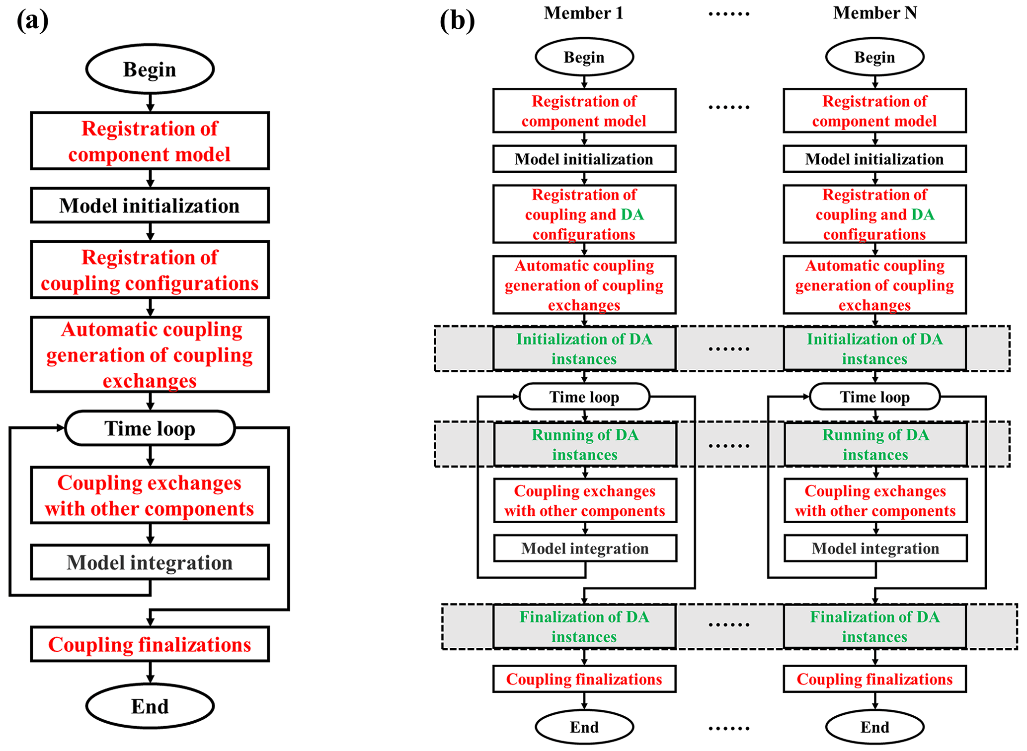
Figure 1 Model flow chart with C-Coupler2.0 (a) and a new model flow chart with ensemble DA based on C-Coupler2.0 (b). Black font indicates the major steps in the original flow chart of a component model without coupling, red font indicates the major steps for achieving coupling exchanges among component models with C-Coupler2.0, and green font indicates the new steps for achieving coupling exchanges between a DA algorithm and a model ensemble. The gray shadow in a dashed rectangle indicates that all members in a model ensemble cooperatively work together for the corresponding step.

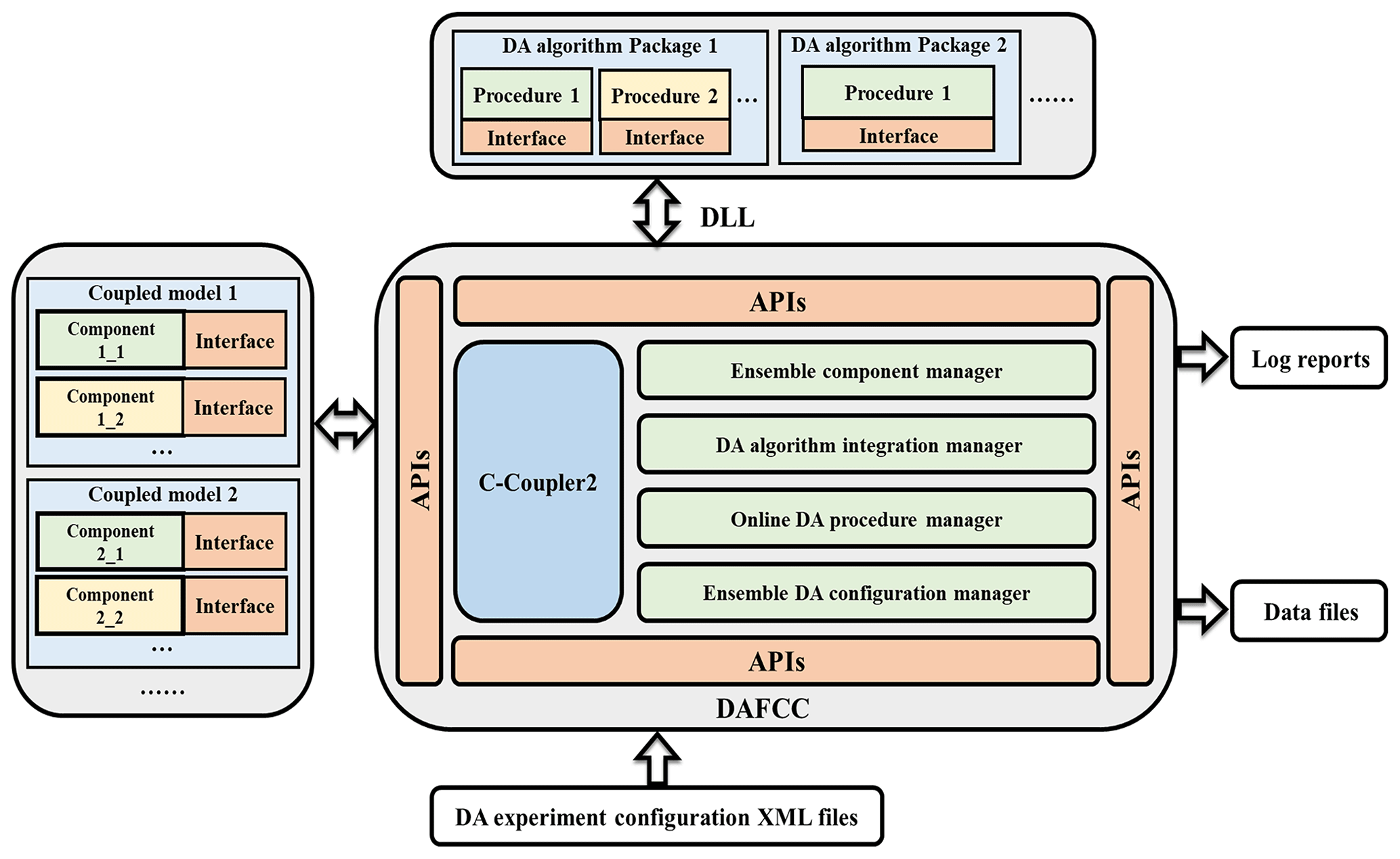
A significant challenge here is that C-Coupler2.0 can only handle coupling exchanges between two component models or within one component model but cannot handle coupling exchanges between a DA algorithm and each model ensemble member. To address this challenge, DAFCC1 automatically generates a special C-Coupler2.0 component model (hereafter called ensemble-set component model) that covers all ensemble members for running a DA algorithm. Thus, coupling exchanges between a DA algorithm and each model ensemble member can be transformed into the coupling exchanges between the ensemble-set component and each ensemble member. Specifically, DAFCC1 introduces three new steps, i.e., initialization, running and finalization of DA instances (instances of DA algorithms), to the model flow chart with C-Coupler2.0 (Fig. 1b). These steps enable a DA instance to run on the processes of all ensemble members and achieve automatic coupling exchanges between a DA algorithm and each model ensemble member. The software architecture of DAFCC1 based on C-Coupler2.0 is shown in Fig. 2. It includes a set of new managers (i.e., DA algorithm integration manager, ensemble component manager, online DA procedure manager, and ensemble DA configuration manager) and the new APIs corresponding to these managers. The DA algorithm integration manager enables the user to conveniently develop driving interfaces for a DA algorithm based on a set of new APIs that enables the DA algorithm to declare its input and output fields and to obtain various information from the model. When a DA algorithm includes multiple independent modules (such as observation operators and analysis modules), each module can be called separately by the model. The dynamic link library (DLL) technique is used to connect a DA algorithm program to a model program. The DA algorithm program is compiled into a DLL that is dynamically linked to a model when an instance of the DA algorithm is initialized. Using the DLL technique allows us to couple a DA algorithm and a model without modifying and recompiling the model code, and it provides greater independence and convenience because the original configuration and compilation systems of the DA algorithm can generally be preserved. The ensemble component manager governs the communicators of ensemble members. The online DA procedure manager provides several APIs that enable the ensemble members of a component model to initialize, run and finalize a DA algorithm instance cooperatively. The data exchanges between the ensemble members and the DA algorithm are also handled automatically in this manager. The ensemble DA configuration manager enables the user to flexibly choose DA algorithms and set parameters for a DA simulation via a configuration file.

Figure 2 Architecture of DAFCC1.

With the software architecture in Fig. 2 and the detailed implementations in Sect. 3, DAFCC1 enables a coupled ensemble DA system to achieve the following features.

1. Each component model can use different instances of DA algorithms online independently, and the execution of a DA algorithm in the MPI processes of a component model does not force other MPI processes to be idled. For example, components 1, 2 and 4 in Fig. 3 perform DA with different time periods (e.g., component 4 performs DA more frequently than component 1 and 2), while component 3 does not use DA algorithms.

2. Given a common DA algorithm, it can be used by different component models under different instances with different configurations (e.g., the fields assimilated, the observational information used and the frequency). In Fig. 3, for example, components 2 and 4 use different instances of the same DA algorithm 2 independently.

3. An instance of a DA algorithm can either use the processes of all ensemble members of the same component model cooperatively or use the processes of each ensemble member separately. For example, each DA algorithm instance in Fig. 3 uses the processes of all ensemble members of the corresponding component model cooperatively, except procedure 1 of DA algorithm 1 that uses the processes of each ensemble member of component 1 separately.

4. Besides employing the DLL technique for integrating DA algorithm programs, a configuration file is designed for increasing the flexibility and convenience in using a DA algorithm (see Sect. 3.4 for detailed implementation).

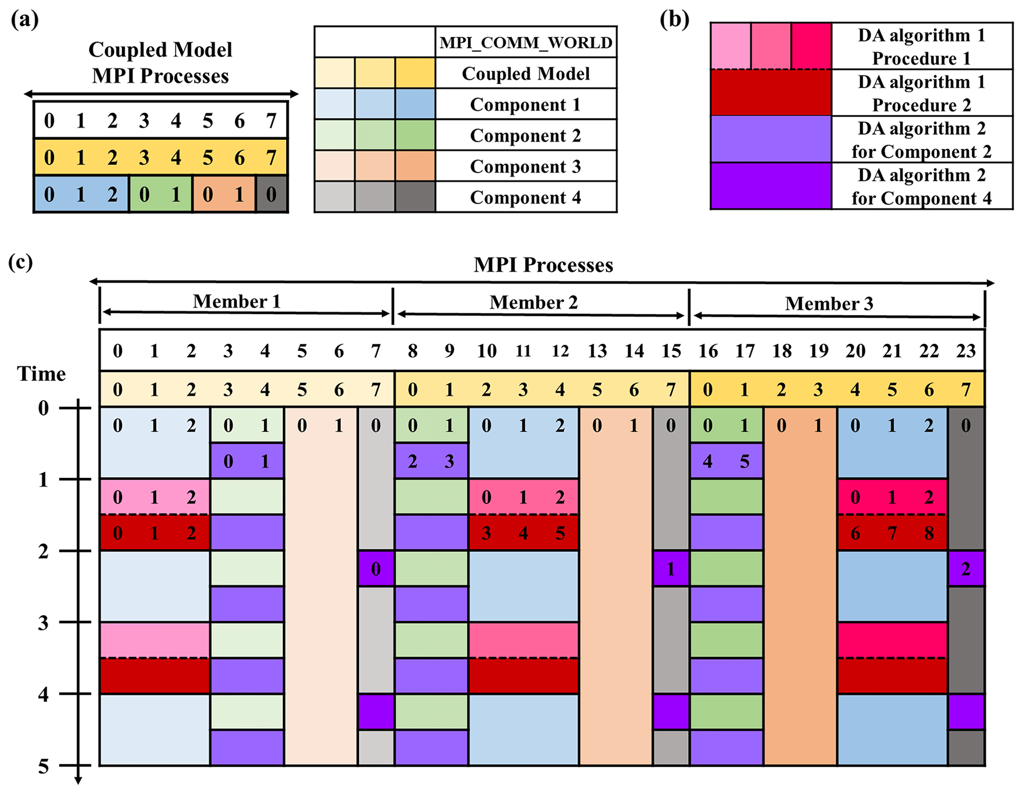
Figure 3 Example of running a DAFCC1-based weakly coupled ensemble DA system with three ensemble members. (a) Each ensemble member of the coupled model (yellow series) uses eight MPI processes, where component 1 (blue series) uses three MPI processes, component 2 (green series) uses two MPI processes, component 3 (orange series) uses two MPI processes and component 4 (gray series) uses one MPI process. (b) DA algorithm 1 and two instances of DA algorithm 2 (purple series) are used in this DA system, where DA algorithm 1 includes procedure 1 (pink series) and procedure 2 (red). (c) Execution of the DA system: the process layout of ensemble members of component models, the process layout of DA algorithms, and the alternative execution of a DA algorithm and the corresponding component model. Each number in the colored box in (a) and (c) indicates the process ID in the corresponding local communicator of a member of the coupled model, a member of a component model or all members of a component model.

3 Implementation of DAFCC1

In this section, we will detail the implementation of DAFCC1 in terms of the ensemble component manager, DA algorithm integration manager, online DA procedure manager and ensemble DA configuration manager. Moreover, we will provide an example of how to use DAFCC1 to develop a DA system.

3.1 Implementation of the ensemble component manager

To achieve coupling exchanges between a DA algorithm and each ensemble member, each ensemble member should be used as a separate component model registered to C-Coupler2.0 via the API CCPL_register_component (Please refer to L. Liu et al., 2018 for more details). In C-Coupler2.0, model names are used as the keywords to distinguish different component models. To distinguish different ensemble members of a model that generally share the same code or executable, we update the API CCPL_register_component to implicitly generate different names of ensemble members by appending the ID of each ensemble member to the model name (the parameter list of the API CCPL_register_component is unchanged). The ID of an ensemble member is given as the last argument (formatted as “CCPL_ensemble_{ensemble numbers}_{member ID}”) of the corresponding executable when submitting an MPI run (see Fig. 4 as an example), where “ensemble numbers” marks the number of ensemble members and “member ID” marks the ensemble member ID of the current component.

Figure 4 Example of the command for submitting an MPI run of three ensemble members of a coupled model that consists of Comp1 and Comp2. Comp1 can be before Comp2 at the second ensemble member, and the process numbers N1_1, N2_1 and N3_1 of Comp1 at different ensemble members can be different.

C-Coupler2.0 can manage hierarchical relationship among models, where a model can have a set of child models. Given an ensemble run of a coupled model, although all ensemble members of all component models of the coupled model can be organized into a single level (see Fig. 5a), we recommend constructing two hierarchical levels (see Fig. 5b), where each ensemble member of the coupled model is at the first level while the component models of each ensemble member are at the second level. This hierarchical organization retains the original architecture of the coupled model and only requires users to simply register the coupled model to C-Coupler2.0.

Figure 5 Two examples of the organization of N ensemble members of a coupled model consisting of M component models. (a) Single-level organizational architecture of all ensemble members of the component models in the coupled model. (b) Two hierarchical level organizational architecture. All ensemble members of the coupled model are organized as the first level with all component models from each ensemble member of the coupled model at the second level. An ensemble-set component model that covers all ensemble members of component model 1 is generated as an example for using the DA algorithm in ensemble component manager.

In order to enable a DA algorithm to run on the MPI processes of all ensemble members of a component model (Fig. 3), an ensemble-set component model that covers all ensemble members of the component model is required for calling the DA algorithm (for example, the green box in Fig. 5b corresponds to an ensemble-set component model). As the ensemble-set component model does not exist in the original hierarchical levels in Fig. 5b, it should be generated with extra efforts. The ensemble component manager provides the capability of automatically generating the corresponding ensemble-set component model when initializing a DA instance. The MPI communicator of the ensemble-set component model is generated through unifying the communicators of the ensemble members of the corresponding component model that runs the DA instance.

3.2 Implementation of the DA algorithm integration manager

When a DA algorithm runs on the processes of a component model, the model and the DA algorithm can be viewed as a caller and a callee in a program, respectively. A callee generally declares a list of arguments that includes a set of input and output variables, and a caller should match the argument list of the callee when calling the callee (a model that calls a DA algorithm is hereafter called the host model of the DA algorithm ). When a caller and a callee are statically linked together, a compiler can generally guarantee the consistency of the argument list between them. However, it is a challenge that compilers cannot guarantee such consistency between a host model and a DA algorithm that is enclosed in a DLL and dynamically linked to the host model.

To address the above challenge, we designed and developed a new solution in DAFCC1 for passing arguments between a host model and a DA algorithm. There are three driving subroutines for initializing, running and finalizing a DA algorithm. These subroutines are enclosed in the same DLL with the DA algorithm. Specifically, names of these subroutines share the name of the DA algorithm as the prefix and are distinguished by different suffixes. We tried to make the explicit argument list of each driving subroutine as simple as possible (e.g., the explicit argument list only includes a few integer arrays) and developed a set of APIs for flexibly passing implicit arguments. Based on these APIs, the DA algorithm can obtain the required information of the host model and can also declare a set of implicit input or output arguments of fields. Figure 6 shows an example of the driving subroutines where the running and finalization driving subroutines are quite simple. The initialization driving subroutine includes the original functionalities of the DA algorithm such as determining parallel decompositions, allocating memory space for variables and other operations for initialization. Moreover, it includes additional operations for obtaining the information of the host model via C-Coupler2.0; registering the parallel decompositions, grids, and field instances to C-Coupler2.0; and declaring a set of field instances as implicit input or output arguments. Data exchanges between the host model and the DA algorithm are conducted automatically and implicitly by DAFCC1 (Sect. 3.3.2), and thus the running driving subroutine DA_CCPL_RUN does not include explicit calls for data exchanges.

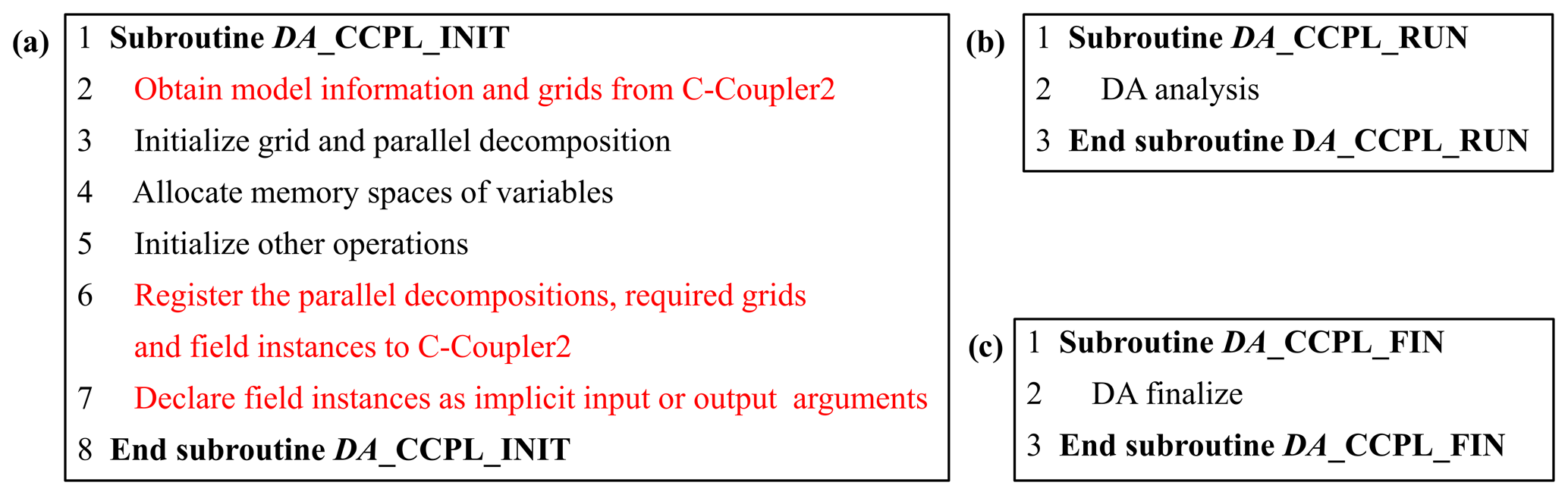
Figure 6 Example of the driving subroutines in a DA algorithm. (a) Initialization driving subroutine. (b) Running driving subroutine. (c) Finalization driving subroutine. The name of the DA algorithm “DA” is used as the prefix of the three driving subroutines; different suffixes are used for distinction. Black font indicates original functionalities of the DA algorithm, while red font indicates additional operations to perform online data exchanges between the model and DA algorithm.

The use of DAFCC1 requires some further changes to the codes of a DA algorithm. For example, the original communicator of the DA algorithm needs to be replaced with the communicator of the host model that can be obtained via the corresponding C-Coupler API, and the original I/O accesses for the model data in the DA algorithm can be turned off.

3.3 Implementation of the online DA procedure manager

To make the same DA algorithm used by different component models, DAFCC1 enables a component model to use a separate instance of the same DA algorithm with the corresponding configuration information. Corresponding to the three driving subroutines of a DA algorithm, there are three APIs (CCPL_ensemble_procedures_inst_init, CCPL_ensemble_procedures_inst_run and CCPL_ensemble_procedures_inst_finalize) that are directly called by the code of a host model. These APIs initialize, run and finalize a DA algorithm instance and handle the data exchanges between the host model and the DA algorithm instance automatically. In a general case in Fig. 1b, the API CCPL_ensemble_procedures_inst_init is called when initializing the ensemble DA system before starting the time loop, the API CCPL_ensemble_procedures_inst_finalize is called after finishing the time loop, and the API CCPL_ensemble_procedures_inst_run is called in the time loop, which enables different assimilation windows to share the same DA instance without restarting the model and the DA algorithm. When a component model initializes, runs or finalizes a DA algorithm instance, all ensemble members of this component model should call the corresponding API at the same time.

3.3.1 API for initializing a DA algorithm instance

The API CCPL_ensemble_procedures_inst_init includes the following steps for initializing a DA algorithm instance.

1. Determining the host model of the DA algorithm instance according to the corresponding information in the configuration file. If the DA algorithm instance is an individual algorithm that operates on the data of each ensemble member separately (e.g., Procedure 1 of DA algorithm 1 in Fig. 3), each ensemble member will be a host model. Otherwise (i.e., the DA algorithm instance is an ensemble algorithm that operates on the data of the ensemble set; e.g., Procedure 2 of DA algorithm 1 in Fig. 3), the host model will be the ensemble-set component model that will be generated automatically by the ensemble component manager.

2. Preparing information from the host model, such as model grids, parallel decompositions, and field instances, which can be obtained by the initialization driving subroutine of the DA algorithm via the corresponding APIs.

3. Initializing the corresponding DA algorithm instance according to the corresponding algorithm name and DLL name specified in the corresponding configuration file (Sect. 3.4), where the corresponding DLL will be linked to the host model and the corresponding initialization-driving subroutine in the DLL will be called. This implementation enables the user to conveniently change the DA algorithms used in different simulations via the configuration file without modifying the code of the model.

4. Setting up data exchange operations according to the input or output fields of the DA algorithm instance declared in the initialization driving subroutine via the corresponding APIs. If the DA algorithm instance is specified as an individual algorithm via the ensemble DA configuration (Sect. 3.4), the data exchange is within each ensemble member. Otherwise, the ensemble-set component model is involved in the data exchange. The data exchange is divided into two levels: (i) the data exchange between the ensemble members and DAFCC1 and (ii) the data exchange between DAFCC1 and the DA algorithm. The data exchange between DAFCC1 and the DA algorithm instance is simply achieved by the import–export interfaces of C-Coupler2.0, which flexibly rearrange the fields in the same component model between different parallel decompositions. If the DA algorithm instance is an ensemble algorithm, the data exchange between the ensemble members and DAFCC1 is also handled by the import–export interfaces of C-Coupler2.0, which flexibly transfer the same fields between different component models (each ensemble member and the ensemble set are different component models). Otherwise, the data exchange between the ensemble members and DAFCC1 is simplified to a data copy. DAFCC1 will hold a separate memory space for each model field relevant to the DA algorithm, which enables a DA algorithm instance to use instantaneous model results or statistical results (i.e., mean, maximum, cumulative, and minimum) in a time window, and enables an ensemble DA algorithm instance to use aggregated results or statistical results (ensemble-mean, ensemble-anomaly, ensemble-maximum or ensemble-minimum) from ensemble members.

Consistent with the functionalities in the above steps, the API CCPL_ensemble_procedures_inst_init includes the following arguments.

• The ID of the current ensemble member that calls this API, and the common full name of the ensemble members. When registering a component model to C-Coupler2.0, its ID is allocated and its unique full name formatted as “parent_full_name@model_name” is generated, where “model_name” is the name of the component model, and “parent_full_name” is the full name of the parent component model (if any). Given that the name of the component model 1 in Fig. 5 is “comp1”, in the one-level model hierarchy in Fig. 5a, the full names of ensemble members of the component model 1 are “comp1_1” to “comp1_N”, and the common full name of the ensemble members is “comp1_*” where “*” is a wildcard, while in the two-level model hierarchy in Fig. 5b, the full names of ensemble members of the component model 1 are “coupled_1@comp1” to “coupled_N@comp1” and the common full name is “coupled_*@comp1” (given that the name of the coupled model is “coupled”). Such a common full name can be used for generating the ensemble-set component model when the DA algorithm instance is an ensemble algorithm.

• The name of the DA algorithm instance, which is the keyword of the DA algorithm instance and also specifies the corresponding configuration information. Different DA algorithm instances can correspond to different DA algorithms or the same DA algorithm. For example, the component models 2 and 4 use different instances of the same DA algorithm in Fig. 3.

• An optional list of model grids and parallel decompositions, which enable the DA algorithm instance to obtain the grid data and use the same parallel decompositions as the host model.

• A list of field instances that can be used for DA. This list should cover all input or output fields of the DA algorithm.

• An optional integer array of control variables that can be obtained by the DA algorithm instance via the corresponding APIs.

• An annotation, which is a string giving a hint for locating the model code of the API call corresponding to an error or warning, is recommended but not mandatory.

3.3.2 API for running a DA algorithm instance

The API CCPL_ensemble_procedures_inst_run includes the following steps for running a DA algorithm instance:

1. Executing the data exchange operations for the input fields of the DA algorithm instance. This step automatically transfers the input fields from each ensemble member of the corresponding component model to DAFCC1 and then from DAFCC1 to the DA algorithm instance. The statistical processing regarding the time window or the ensemble is done at the same time.

2. Executing the DA algorithm instance through calling the running driving subroutine of the DA algorithm.

3. Executing the data exchange operations for the output fields of the DA algorithm instance. This step automatically transfers the output fields from the DA algorithm instance to DAFCC1 and then from DAFCC1 to each ensemble member of the corresponding component model.

Each DA algorithm instance has a timer specified via the configuration information, which determines when the DA algorithm instance is run. The API CCPL_ensemble_procedures_inst_run for a DA algorithm instance can be called at each time step, while the above three steps will be executed only when the specified timer is on. To store the input data such as the observational information, a DA algorithm instance can either share the working directory of its host model or use its own working directory specified via the configuration information. The API CCPL_ensemble_procedures_inst_run will change and then recover the current directory for calling the running driving subroutine of the DA algorithm if necessary.

3.3.3 API for finalizing a DA algorithm instance

The API CCPL_ensemble_procedures_inst_finalize is responsible for finalizing a DA algorithm instance through calling the finalization driving subroutine of the DA algorithm.

3.4 Implementation of the ensemble DA configuration manager

The configuration information of all DA algorithm instances used in a coupled DA simulation is enclosed in an XML configuration file (e.g., Fig. 7). Each DA algorithm instance has a distinct XML node (e.g., the XML node “da_instance” in Fig. 7, where the attribute “name” is the name of the DA algorithm instance associated with the API “CCPL_ensemble_procedures_inst_init”), which enables the user to specify the following configurations.

1. The DA algorithm specified in the XML node “external_procedures” in Fig. 7. The attribute “dll_name” in the XML node specifies the dynamic link library, and the attribute “procedures_name” specifies the DA algorithm's name associated with the corresponding driving subroutines. When the user seeks to change the DA algorithm used by a component model, it is only necessary to modify the XML node “external_procedures” in most cases.

2. The periodic timer specified in the XML node “periodic_timer” in Fig. 7, which enables the user to flexibly set the periodic model time of running the corresponding DA algorithm. Besides the attribute “period_unit” and “period_count” for specifying the period of the timer, the user can specify a lag via the attribute “local_lag_count”. For example, given a periodic timer <“period_unit”=“hours”, “period_count”=6, “local_lag_count”=3>, its period is 6 h, and it will not be on at the 0th, 6th, and 12th hours but instead on at the 3rd, 9th, and 15th hours due to the “local_lag_count” of 3.

3. Statistical processing of input fields specified in the XML node “field_instances” in Fig. 7. The attribute “time_processing” specifies the statistical processing in each time window determined by the periodic timer. The attribute “ensemble_operation” specifies the statistical processing among ensemble members. For an individual DA algorithm, the attribute “ensemble_operation” should be set to “none”. All fields can share the default specification of statistical processing, while a field can have its own statistical processing specified in a sub node of the XML node “field_instances”.

4. The working directory and the scripts for pre- and post-assimilation analysis (e.g., for processing the data files of observational information) optionally specified in the XML node “processing_control” in Fig. 7. When the working directory is not specified, the DA algorithm instance will use the working directory of its host model. The script specified in the sub XML node “pre_instance_script” will be called by the root process of the host model before the API CCPL_ensemble_procedures_inst_run calls the DA algorithm, and the script specified in the sub XML node “post_instance_script” will be called by the root process of the host model after the DA algorithm run finishes.

Figure 7 Example of the XML configuration for a DA experiment.

4 An example weakly coupled ensemble DA system based on DAFCC1

To provide further information on how to use DAFCC1 and for validating and evaluating DAFCC1, we developed an example weakly coupled ensemble DA system by combining the ensemble DA system GSI/EnKF (Shao et al., 2016; H. Liu et al., 2018) and a regional First Institute of Oceanography Atmosphere–Ocean–Wave (FIO-AOW) coupled model (Zhao et al., 2017; Wang et al., 2018). GSI/EnKF mainly focuses on regional numerical weather prediction (NWP) applications coupled with the Weather Research and Forecasting (WRF) model (Wang et al., 2014), while FIO-AOW consists of WRF, the Princeton Ocean Model (POM; Blumberg and Mellor 1987; Wang et al., 2010), the MArine Science and NUmerical Modeling wave model (MASNUM; Yang et al., 2005; Qiao et al, 2016), and all the above three model components are coupled together by using C-Coupler (L. Liu et al., 2014, 2018). FIO-AOW has already been used in the research for exploring the sensitivity of typhoon simulation to physical processes and improving typhoon forecasting (Zhao et al, 2017; Wang et al., 2018). There are two main steps in developing the example system.

We developed an ensemble DA sub-system of WRF by adapting GSI/EnKF to DAFCC1. This sub-system helps validate DAFCC1 and evaluate the improvement in performance obtained by DAFCC1 (Sect. 5).

We merged the above sub-system and FIO-AOW to produce the example DA system that only computes atmospheric analyses corresponding to WRF currently. This system demonstrates the correctness of DAFCC1 in developing a weakly coupled ensemble DA system.

4.1 An ensemble DA sub-system of WRF

4.1.1 Brief introduction to GSI/EnKF

GSI/EnKF combines a variational DA sub-system (GSI; Shao et al., 2016) and an ensemble DA sub-system (EnKF; H. Liu et al., 2018), which can be used as a variational, a pure ensemble or a hybrid DA system sharing the same observation operator in the GSI codes. It provides two options for calculating analysis increments for ensemble DA; i.e., a serial ensemble square root filter (EnSRF) algorithm (Whitaker et al., 2012) and a local ensemble Kalman filter (LETKF) algorithm (Hunt et al., 2007). In this paper, we use the pure ensemble DA system without using variational DA, where GSI is used as the observation operator that calculates the difference between model variables and observations on the observation space and EnSRF is chosen for calculating atmospheric analyses and updating atmosphere model variables.

Figure 8a shows the flow chart for running the pure ensemble DA system of the WRF model in a DA window. It consists of the following main steps that are driven by scripts, while the data exchanges between these main steps are achieved via data files.

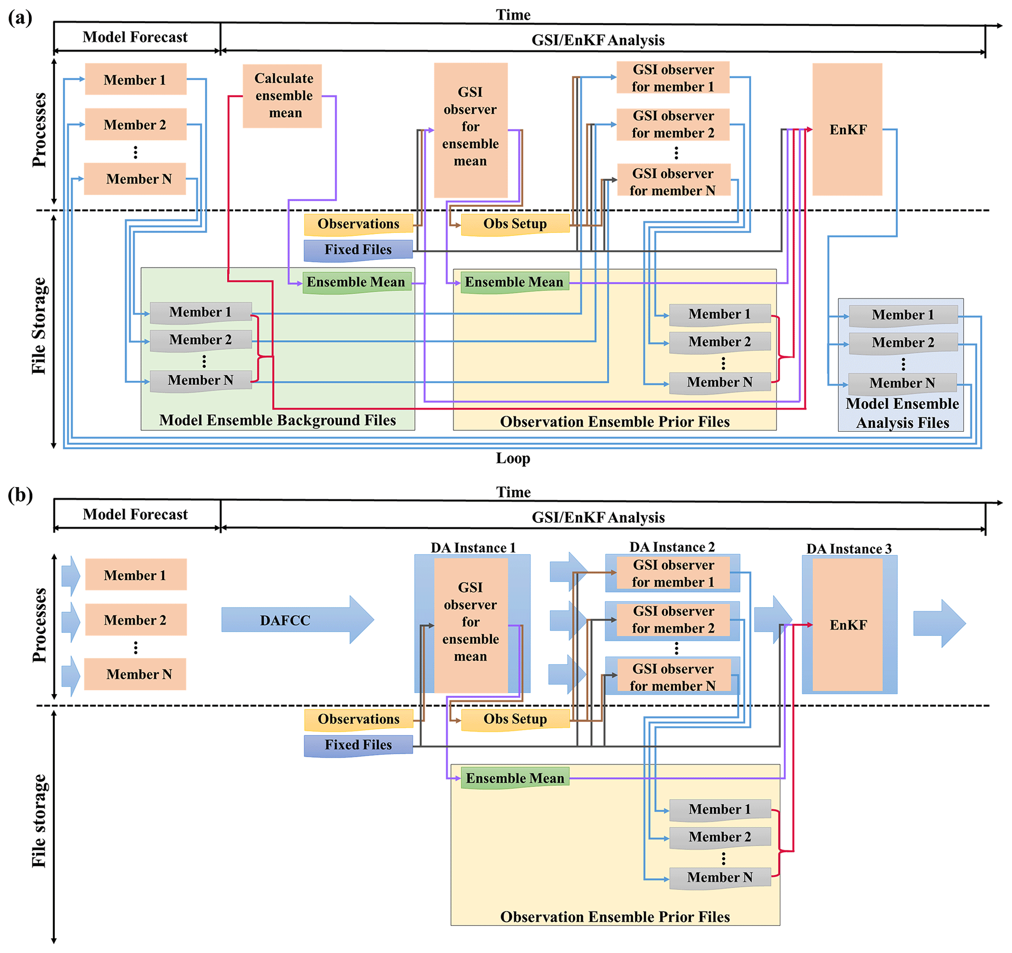
Figure 8 Running processes and data scheduling for (a) original GSI/EnKF used as a pure ensemble DA system and (b) modified GSI/EnKF based on DAFCC1. Orange rectangles in the processes panel indicate different running processes, while thick blue arrows mark data scheduling based on DAFCC1. Rectangles of various colors with a curved lower edge in the file storage panel indicate different files, while arrows of different colors indicate the scheduling of corresponding files.

Ensemble model forecast. An ensemble run of WRF is initiated or restarted from a set of input data files and is then stopped after producing a set of output files (called model background files hereafter) for DA and for restarting the ensemble run in the next DA window.

Calculating the ensemble mean of model DA variables. A separate executable is initiated for calculating the ensemble mean of each DA variable based on the model background files and then outputs the ensemble mean to a new background file.

Observation operator for the ensemble mean. GSI is initiated as the observation operator for the ensemble mean. It takes the ensemble mean file, files of various observational data (e.g., conventional data, satellite radiance observations, GPS radio occultations, and radar data) and multiple fixed files (e.g., statistic files, configuration files, bias correction files, and Community Radiative Transfer Model coefficient files) as input and produces an observation prior (observation innovation) file for the ensemble mean and files containing observational intermediate information (e.g., bias correction and thinning).

Observation operator for each ensemble member. GSI is initiated as the observation operator for each ensemble member. It takes the background file of the corresponding ensemble member, the fixed files and the observational intermediate information files as input and produces an observation prior file for the corresponding ensemble member.

EnKF for calculating analysis increments. EnKF is initiated for calculating analysis increments of the whole ensemble. It takes the model background files, the observation prior files and the fixed files as input, and finally updates model background files with the analysis increments. The updated model background files are used for restarting the ensemble model forecast in the next DA window.

4.1.2 Adapting GSI/EnKF to DAFCC1

When adapting GSI/EnKF to DAFCC1, an ensemble-set component model derived from the ensemble forecast of WRF (corresponding to the first main step in Sect. 4.1.1) is generated as the host model that drives the DA algorithm instances corresponding to the remaining main steps. As shown in Fig. 9, three DA instances corresponding to the last three main steps in Sect. 4.1.1 (i.e., observation operator for the ensemble mean, observation operator for each ensemble member and EnKF for calculating analysis increments) are enclosed in DLLs, without a DA algorithm instance corresponding to the second main step in Sect. 4.1.1. This is because the online DA procedure manager of DAFCC1 enables a DA algorithm instance to automatically obtain the ensemble mean of model DA variables (Sect. 3.3). Although both the third and fourth main steps correspond to the same GSI, they are transformed into two different DA algorithm instances because the third is an ensemble algorithm (i.e., it operates on the data of the ensemble set) and the fourth is an individual algorithm (i.e., it operates on the data of each ensemble member). Moreover, we compiled the same GSI code into two separate DLLs, each of which corresponds to one of these two instances, to enable these two instances to use different memory space.

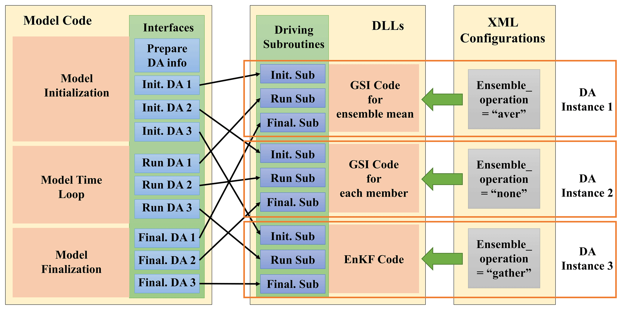
Figure 9 Modifications of model code and the invoking of relationships to the DA algorithm in the example ensemble DA system.

For each DA algorithm instance, three driving subroutines and the corresponding configuration were developed (Fig. 9). In fact, the two instances corresponding to GSI share the same driving subroutines but use different configurations (especially regarding the specification of “ensemble_operation”). To enable the GSI code and EnKF code to be used as DLL, we made the following slight modifications to the code.

We turned off the MPI initialization and finalized and replaced the original MPI communicator with the MPI communicator of the host model that can be obtained via DAFCC1.

We obtained the required model information and the declared input/output fields via DAFCC1, and turned off the corresponding I/O accesses.

To drive the DA algorithm instances, the WRF code was updated with the new subroutines for initializing, running and finalizing all DA algorithm instances. Moreover, the functionality of outputting model background files can be turned off because the data exchanges between WRF and the DA algorithm instances are automatically handled by DAFCC1 and the WRF ensemble can be run continuously throughout DA windows without stopping and restarting. As a result, DAFCC1 saves sets of data files and the corresponding I/O access operations, while only the observation files, fixed files, and the files for the data exchanges among the DA algorithm instances are reserved (compare Fig. 8b and a).

4.2 Example ensemble DA system of FIO-AOW

FIO-AOW, which previously used C-Coupler1 (Liu et al., 2014) for model coupling, has already been upgraded to C-Coupler2.0 by us (Fig. 10a). As GSI/EnKF and FIO-AOW share WRF, the development of the example ensemble DA system of FIO-AOW in Fig. 10b can significantly benefit from the DA system of WRF. In this ensemble DA system, the ensemble of WRF computes atmospheric analyses based on the ensemble DA sub-system in Sect. 4.1, while each ensemble member of other component models is impacted by the atmospheric analyses via model coupling. It only took the following steps to construct the example ensemble DA system.

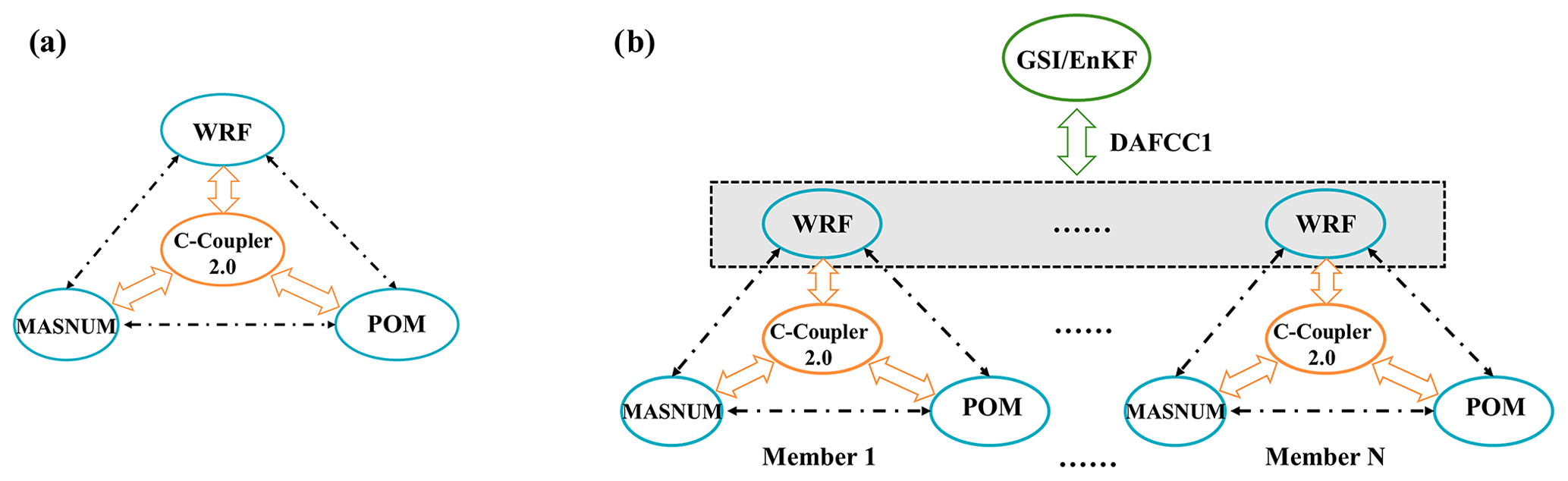
Figure 10 Architecture of FIO-AOW (a) and the corresponding example ensemble DA system (b). The gray shadow in the dashed rectangle in (b) indicates that atmospheric analyses are computed by GSI/EnKF that has been coupled with the ensemble of WRF based on DAFCC1.

Using the ensemble component manager, set up the two hierarchical levels of models shown in Fig. 11; i.e., the first level corresponds to all ensemble members of FIO-AOW while each member includes its three component models at the second level.

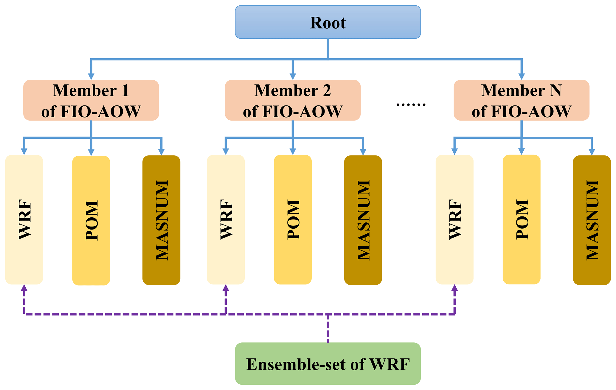
Figure 11 Two-hierarchical-level organizational architecture for N ensemble members of FIO-AOW consisting of WRF, POM and MASNUM. All ensemble members of FIO-AOW are organized as the first level with all component models in each ensemble member at the second level. An ensemble-set that covers all ensemble members of the component model WRF is generated by the ensemble component manager.

Merge the model code modifications, the DA algorithm instances and configurations in the DA system of WRF into the example ensemble DA system FIO-AOW.

As well as being described by the flow chart involving the WRF and the DA algorithm instances in Fig. 8b, the example ensemble DA system of FIO-AOW follows the process layout in Fig. 12, which is essentially a real case of the process layout in Fig. 3.

Figure 12 Example of the process layout of the example ensemble DA system FIO-AOW. (a) Each ensemble member of FIO-AOW (yellow series) uses seven MPI processes, where WRF (blue series) uses three MPI processes, POM (green series) uses two MPI processes, and MASNUM (orange series) uses two MPI processes. (b) Two DA algorithm instances of GSI are adopted for each member (pink series) and ensemble mean (red), respectively, following another DA algorithm instance of EnKF in this DA system. (c) Process layout of the DA system: the process layout of ensemble members of component models and the process layout of DA algorithms. Each number in the colored boxes in (a) and (c) indicates the process ID in the corresponding local communicator of a member of the coupled model, a member of a component model or all members of a component model.

5 Validation and evaluation of DAFCC1

In this section, we evaluate the correctness of DAFCC1 in developing a weakly coupled ensemble DA system based on the example ensemble DA system (hereafter referred to as the full example DA system) described in Sect. 4, and will also validate DAFCC1 and evaluate the impact of DAFCC1 in accelerating DA based on the sub-system with WRF and GSI/EnKF (hereafter WRF-GSI/EnKF).

5.1 Experimental setup

The example ensemble DA system used in this validation and evaluation consists of WRF Version 4.0 (Wang et al., 2014), GSI version 3.6 and EnKF version 1.2, and the corresponding versions of POM and MASNUM used in FIO-AOW (Zhao et al., 2017; Wang et al., 2018). In EnKF version 1.2 the default settings are used; i.e., the EnSRF algorithm is used to calculate analysis increments for ensemble DA, the inflation factor is 0.9 without smoothing, and the covariance is localized by distance correlation function with a horizontal localization radius of 400 km and vertical localization scale coefficient of 0.4. The example ensemble DA system is run on a supercomputer of the Beijing Super Cloud Computing Center (BSCC) with the Lustre file system. Each computing node on the supercomputer includes two Intel Xeon E5-2678 v3 CPUs (Intel(R) Xeon(R) CPU), with 24 processor cores in total, and all computing nodes were connected with an InfiniBand network. The codes were compiled by an Intel Fortran and C$++$ compiler at the optimization level O2 using an Intel MPI library. A maximum 3200 cores are used for running the example ensemble DA system.

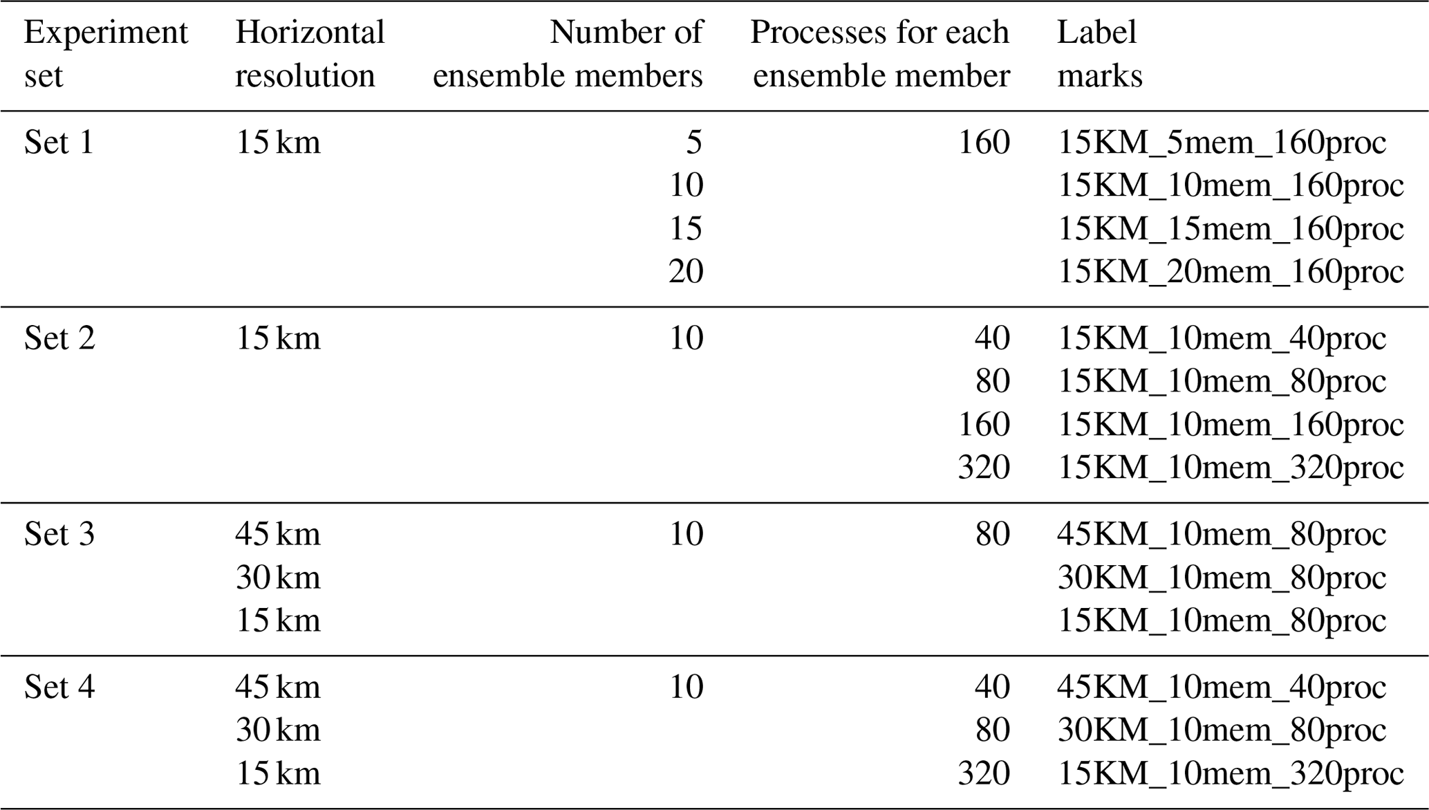
The WRF-GSI/EnKF integrates over an approximate geographical area generated from a Lambertian projection of the area 0–50^∘ N, 99–160^∘ E, with center point at 35^∘ N, 115^∘ E. Initial fields and lateral boundary conditions (at 6 h intervals) for the ensemble run of WRF are taken from the NCEP Global Ensemble Forecast System (GEFS) (at 1^∘ × 1^∘ resolution) (https://www.ncdc.noaa.gov/data-access/model-data/model-datasets/global-ensemble-forecast-system-gefs, last access: 15 April 2020). To configure WRF, an existing physics suite “CONUS” (https://www2.mmm.ucar.edu/wrf/users/physics/ncar_convection_suite.php, last access: 7 May 2021) and 32 vertical sigma layers with the model top at 50 hPa are used. A 1 d integration on 1 June 2016 is used for running the WRF-GSI/EnKF. NCEP global GDAS Binary Universal Form for the Representation of meteorological data (BUFR; https://www.emc.ncep.noaa.gov/mmb/data_processing/NCEP_BUFR_File_Structure.htm, last access: 15 April 2020) and Prepared BUFR (https://www.emc.ncep.noaa.gov/mmb/data_processing/prepbufr.doc/document.htm, last access: 15 April 2020), including conventional observation data and satellite radiation data, are assimilated every 6 h (i.e., at 00:00, 06:00, 12:00, and 18:00 UTC). The air temperature (T), specific humidity (QVAPOR), longitude and latitude wind (UV), and column disturbance dry air quality (MU) are the variables analyzed in the data assimilation. The WRF-GSI/EnKF experiments are classified into four sets, where variations of horizontal resolution (and the corresponding time step), number of ensemble members and process number (each process runs on a distinct processor core) are considered (Tables 1 and 2).

Table 1 Horizontal resolutions and time steps of WRF.

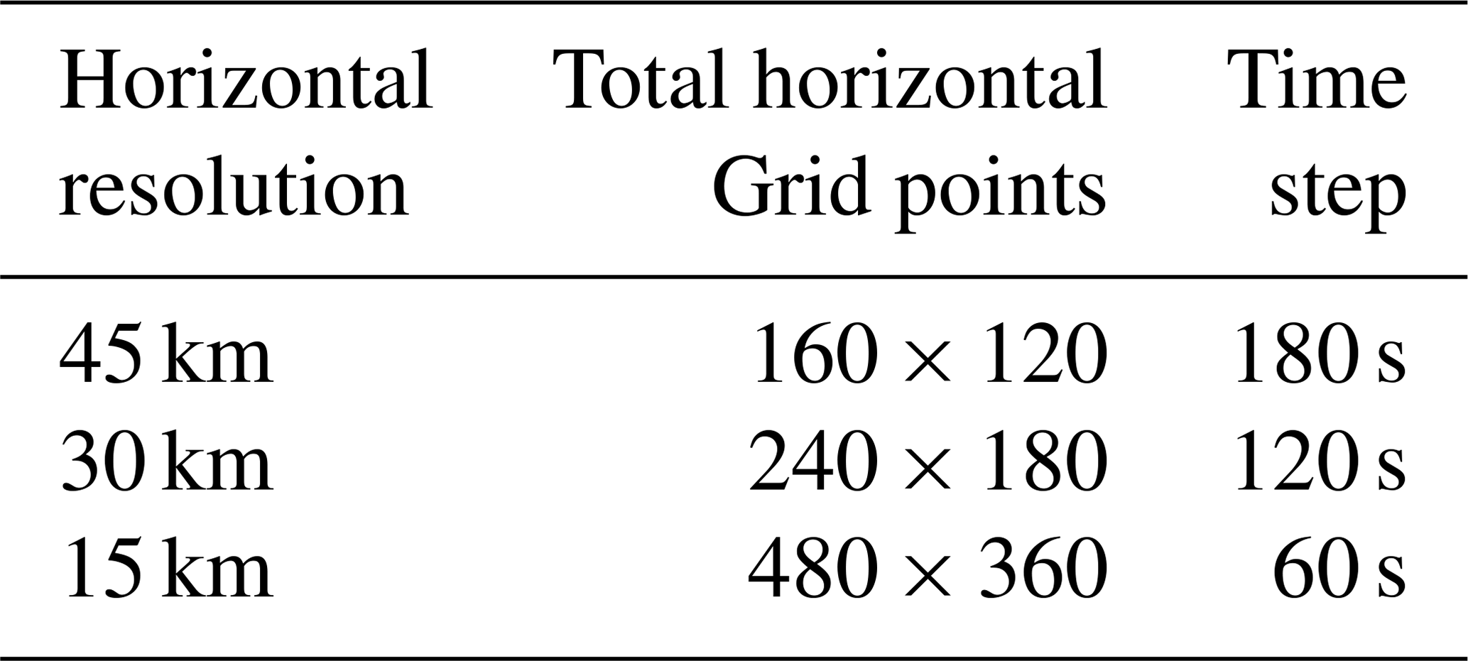
Table 2 Setup of four experiment sets in terms of horizontal resolution, number of ensemble members and number of processes.

All component models of the full example DA system integrate over the same geographical area (0–50^∘ N, 99–150^∘ E) with the same horizontal resolution of $\mathrm{0.5}{}^{\circ }\times \mathrm{0.5}{}^{\circ }$ but different time steps (100 s for WRF and 300 s for POM and MASNUM, coupled by C-Coupler2.0 at 300 s intervals). More details of the model configurations can be found in Zhao et al. (2017). The configuration of initial fields, lateral boundary conditions and observations of WRF for the ensemble run of the full example DA system are the same as for WRF-GSI/EnKF. The full example DA system integrates over 3 d (1 to 3 June 2016), while the first model day is considered as spin-up, and DA is performed every 6 h in the last two model days with T, UV and MU as DA variables.

5.2 Validation of DAFCC1

To validate DAFCC1, we compare the outputs of the two versions of WRF-GSI/EnKF: the original WRF-GSI/EnKF (hereafter offline WRF-GSI/EnKF; https://dtcenter.org/community-code/gridpoint-statistical-interpolation-gsi/community-gsi-version-3-6-enkf-version-1-2, last access: 15 April 2020) and the new version of WRF-GSI/EnKF with DAFCC1 (hereafter online WRF-GSI/EnKF) introduced in Sect. 4.1. As DAFCC1 only improves the data exchanges between a model and the DA algorithms, the simulation results of an existing DA system should not change when it is adapted to use DAFCC1. We therefore employ a validation standard that the WRF-GSI/EnKF with DAFCC1 keeps bit-identical result with the original offline WRF-GSI/EnKF. DAFCC1 passes the validation test with all experimental setups in Table 2, where the binary data files output by WRF at the end of the 1 d integration are used for the comparison.

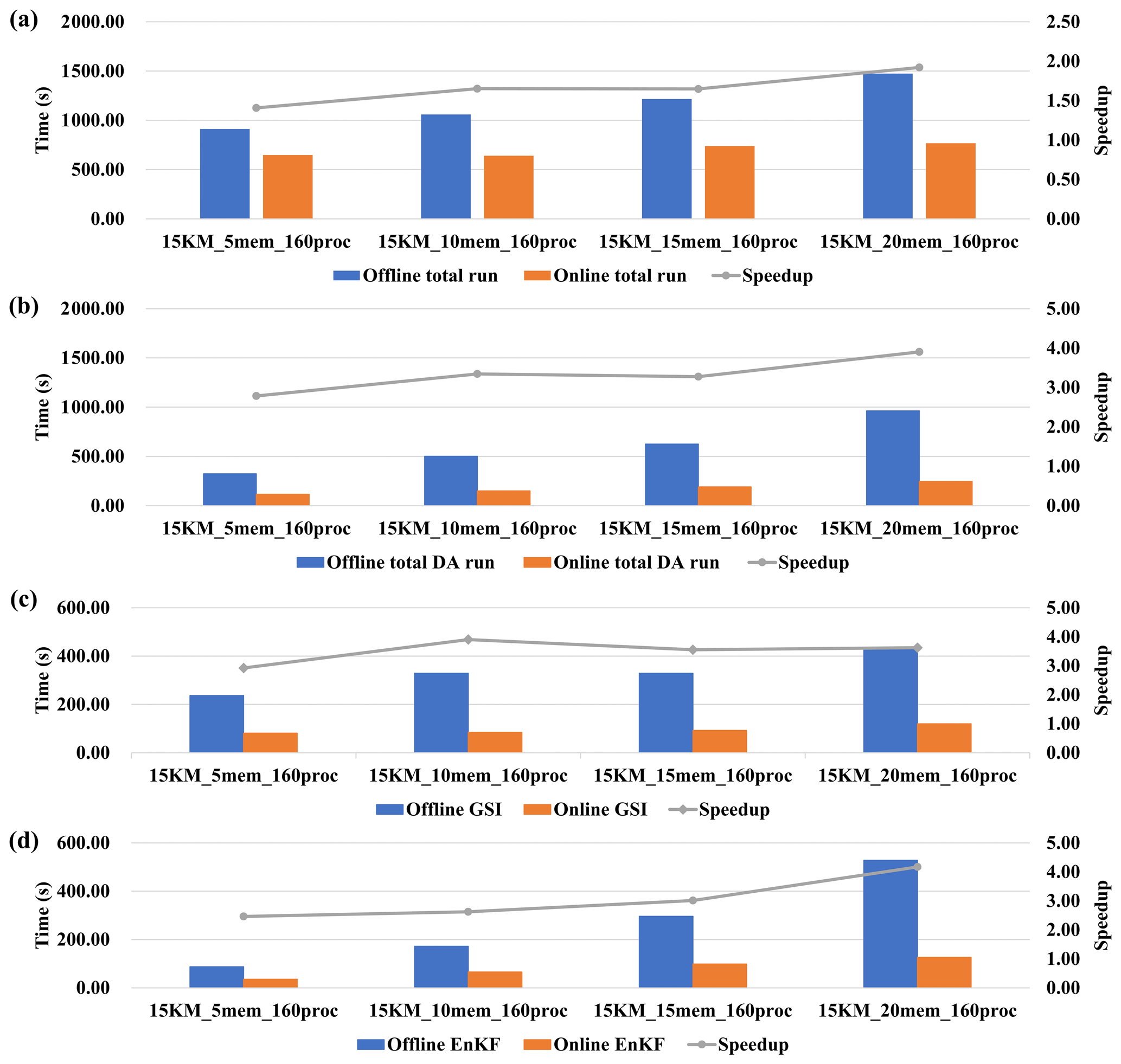
Figure 13 Execution time (colored bars) corresponding to the online and offline WRF-GSI/EnKF and the corresponding speedup (gray line, ratio of offline execution time to online execution time) from experiment set 1 in Table 2. (a) Total run (including model run and DA algorithms run). (b) DA algorithms (including GSI and EnKF) run. (c) GSI run. (d) EnKF run.

5.3 Impact in accelerating an offline DA

WRF-GSI/EnKF is further used to evaluate the impact of DAFCC1 in accelerating an offline DA by comparing the execution time of the offline and online WRF-GSI/EnKF under each experimental setup in Table 2. Considering that all ensemble members of the online WRF-GSI/EnKF are integrated simultaneously, we run all ensemble members of the offline WRF-GSI/EnKF concurrently through a slight modification to the corresponding script in order to make a fair comparison.

Figure 14 The same as in Fig. 13 but from experiment set 2 in Table 2.

Figure 15 The same as in Fig. 13 but from experiment set 3 in Table 2.

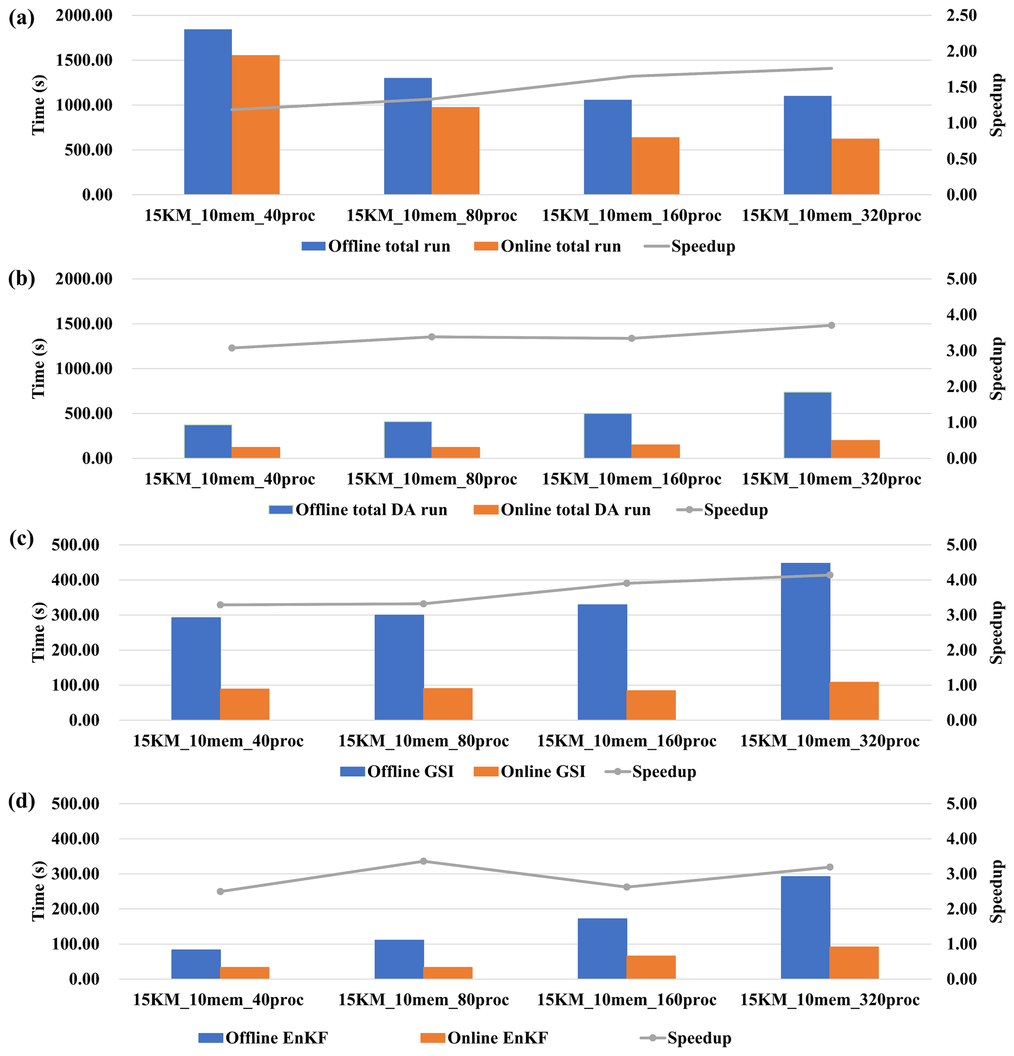
The impact of varying the number of ensemble members is evaluated based on set 1 in Table 2. DAFCC1 obviously accelerates WRF-GSI/EnKF and can achieve higher performance speedup with more ensemble members (Fig. 13a). This is because DAFCC1 significantly accelerates the DA for both GSI and EnKF (Fig. 13b–d). Similarly, DAFCC1 significantly accelerates the DA and WRF-GSI/EnKF under different process numbers (Fig. 14, corresponding to set 2 in Table 2) and resolution (Fig. 15, corresponding to set 3 in Table 2). Considering that more processor cores are generally required to accelerate the model run under higher resolution, we also make an evaluation based on set 4 in Table 2, where concurrent changes in resolution and process number are made to achieve similar numbers of grid points per process throughout the experimental setups. This evaluation also demonstrates the correctness of DAFCC1 in accelerating the DA and WRF-GSI/EnKF (Fig. 16).

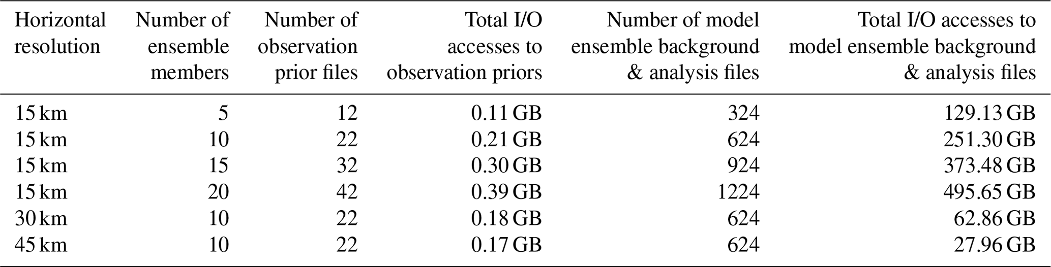
The performance speedups observed from Figs. 11–14 result mainly from the significant decrease in I/O accesses. Although the online WRF-GSI/EnKF still has to access the observation prior files (Sect. 4.1.1 and Fig. 8b), most I/O accesses correspond to the model ensemble background files and model ensemble analysis files, and these I/O accesses have been eliminated by DAFCC1 (Table 3). Moreover, more I/O accesses can be saved under higher-resolution or more ensemble members.

Table 3 I/O access statistics corresponding to WRF-GSI/EnKF.

We note that the execution time of the offline GSI in Fig. 13c increases when using more ensemble members. This is reasonable because more ensemble members introduce more I/O accesses, as shown in Table 3. We also note that the execution time of the offline and online EnKF in Figs. 13d and 14 increases when using more ensemble members. This is because the current parallel version of EnKF does not achieve good scaling performance, and thus longer execution times can be observed when EnKF uses more processor cores.

5.4 Correctness in developing a weakly coupled ensemble DA system

We have successfully run the full example DA system with 10 ensemble members, which enables us to investigate the model fields before and after DA. We find that changes to the atmospheric fields resulting from DA can be observed: for example, the bias regarding T is slightly decreased and the bias regarding UV is more obviously decreased after using DA, as shown in Fig. 17.

Figure 16 The same as in Fig. 13 but from experiment set 4 in Table 2.

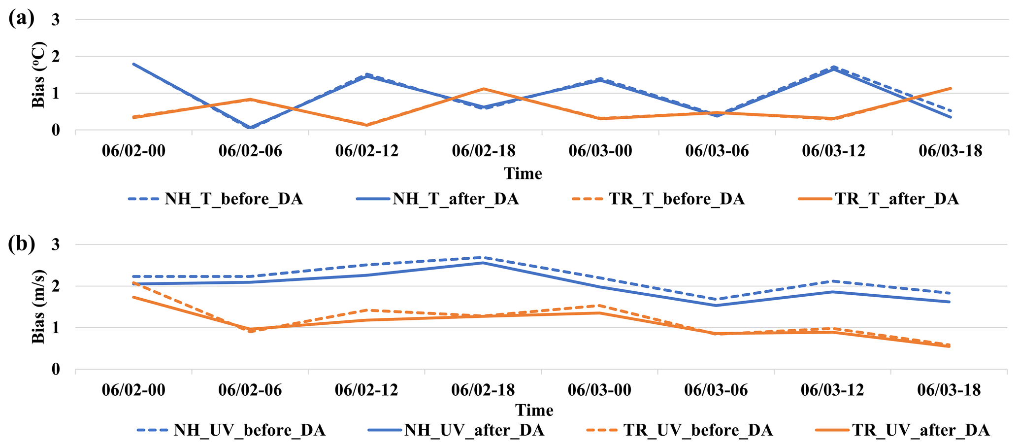
Figure 17 Total bias of assimilated variables relative to corresponding observations before and after DA for (a) T and (b) UV at each DA time from the EnKF standard output file. The dotted lines indicate the bias of assimilated variables before DA, and the solid lines indicate the bias of assimilated variables after DA. Blue lines are the bias in the area of 0–25^∘ N, and orange lines are the bias in the area of 25–50^∘ N.

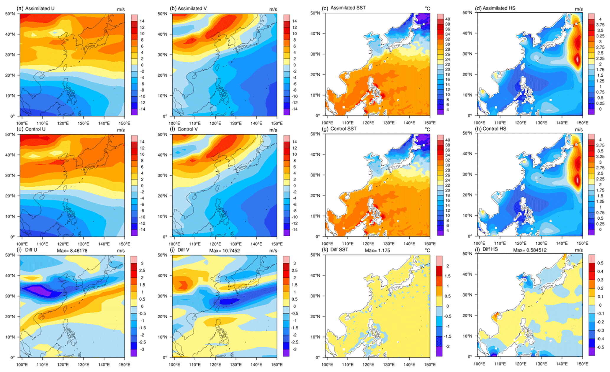
Figure 18 Simulation results of FIO-AOW (at 06:00 UTC on 3 June 2016) about the fields of meridional wind (U; the first column) and zonal wind (V; the second column) produced by WRF, sea surface temperature (SST; the third column) produced by POM, and sea surface significant wave height (HS; the fourth column) produced by MASNUM. The first row shows the results of the full example DA system predicted since 00:00 UTC on 3 June, based on the DA experimental setup in Sect. 5.1, the second row shows the results without DA, and the third row is the corresponding differences.

Changes to the atmospheric fields predicted based on the initial fields updated with the atmospheric analyses can also be observed (e.g., the fields U and V in Fig. 18). Although only atmospheric analyses are computed currently, the model coupling in the weakly coupled DA system makes ocean and wave fields become impacted by the atmospheric analyses, and therefore changes to the ocean and wave fields can be observed in a prediction (e.g., the fields SST and HS in Fig. 18).

6 Conclusions and discussion

In this paper, we propose a new common, flexible and efficient framework for weakly coupled ensemble data assimilation based on C-Coupler2.0, DAFCC1. It provides simple APIs and a configuration file format to enable users to conveniently integrate a DA method into a model as a procedure that can be directly called by the model, while still guaranteeing the independence of configuration and compilation systems between the model and the DA method. The example weakly coupled ensemble DA system in Sect. 4 and the evaluations in Sect. 5 demonstrate the correctness of DAFCC1 in both developing a weakly coupled ensemble DA system and accelerating an offline DA system. The development of a DA system that only employs a single model run but not an ensemble run can also benefit from the advantages of DAFCC1, while the functionality of data exchanges will be automatically simplified without generating ensemble-set component models for saving extra overhead.

DAFCC1 is able to automatically handle data exchanges between a model ensemble and a DA algorithm because its design and implementation significantly benefit from C-Coupler2.0, which already has the functionalities of automatic coupling generation and automatic data exchanges between different component models or within the same component model. DAFCC1 will therefore be an important functionality of the next generation of C-Coupler (C-Coupler3) that is planned to be released no later than 2022. Although the example ensemble DA system of FIO-AOW developed in this work only computes atmospheric analyses currently, the future work similar to adapting GSI/EnKF to DAFCC1 can be conducted to further enable the computation of ocean or wave analyses. Moreover, we have considered software extendibility when designing and implementing DAFCC1, which will enable us to conveniently achieve upgrades either for strongly coupled ensemble DA systems or for more types of data exchange operations in the future. As shown in Fig. 8, the I/O accesses to the observation prior files for the data exchanges between DA algorithms are still retained after using DAFCC1. Although they are not currently a performance bottleneck (Table 3), we will investigate how to avoid these types of I/O accesses when further upgrading DAFCC1.

Regarding the evaluations in Sect. 5, we can only use at most 3200 processor cores, which limits the maximum number of cores per ensemble member. Consequently, we use relatively coarse resolutions of WRF and FIO-AOW. However, the results in Fig. 16 from the experiment set 4 in Table 2 indicate that DAFCC1 will also obviously accelerate the DA system when using a finer resolution and more processor cores, because it will also significantly decrease I/O accesses. DAFCC1 can tackle the technical challenges in developing or accelerating a DA system but cannot contribute to improvements in simulation results that generally depend on scientific settings that must be determined in the research environment (e.g., the DA algorithm configuration, the inflation factor, localization settings, initial states of the model ensemble run). Consequently, we did not examine the improvements in simulation results resulting from the full example DA system based on various variables in Sect. 5.4 but only made a simple comparison of simulation results, demonstrating that the full example DA system can successfully run and produce simulation results.

The offline implementation of a DA system that relies on disk files and restart functionalities of models and DA algorithms can be a robust strategy when it comes to massively parallel computing where the risk of random task failures generally increases with more processor cores being used by a task because a failed task that corresponds to an ensemble member can be resumed from the corresponding restart files. The online implementation that unifies all ensemble members into a task enables us to significantly increase the number of cores used by a task. At the same time as enlarging the risk of random task failures, the online implementation can decrease such risks because it can significantly reduce disk file accesses that are generally an important source of task failures. The robustness of an online implementation can be further improved through developing the restart capability of the DA system based on the restart capabilities of the model and C-Coupler2, while users are enabled to flexibly set the restart file writing frequency for the online implementation, which can be lower than the corresponding frequency for an online implementation generally determined by observation data frequencies. Moreover, the impact of the overhead of writing restart files in an online implementation can be further decreased via asynchronous I/O support.