Snow profile alignment and similarity assessment for aggregating, clustering, and evaluating snowpack model output for avalanche forecasting

Snowpack models simulate the evolution of the snow stratigraphy based on meteorological inputs and have the potential to support avalanche risk management operations with complementary information relevant for their avalanche hazard assessment, especially in data-sparse regions or at times of unfavorable weather and hazard conditions. However, the adoption of snowpack models in operational avalanche forecasting has been limited, predominantly due to missing data processing algorithms and uncertainty around model validity. Thus, to enhance the usefulness of snowpack models for the avalanche industry, numerical methods are required that evaluate and summarize snowpack model output in accessible and relevant ways. We present algorithms that compare and assess generic snowpack data from both human observations and models, which consist of multidimensional sequences describing the snow characteristics of grain type, hardness, and age. Our approach exploits Dynamic Time Warping, a well-established method in the data sciences, to match layers between snow profiles and thereby align them. The similarity of the aligned profiles is then evaluated by our independent similarity measure based on characteristics relevant for avalanche hazard assessment. Since our methods provide the necessary quantitative link to data clustering and aggregating methods, we demonstrate how snowpack model output can be grouped and summarized according to similar hazard conditions. By emulating aspects of the human avalanche hazard assessment process, our methods aim to promote the operational application of snowpack models so that avalanche forecasters can begin to build an understanding of how to interpret and trust operational snowpack simulations.

1 Introduction

Snow avalanches are a serious mountain hazard, whose risk is managed through a combination of long- and short-term mitigation measures, depending on the character of the exposed elements at risk. Avalanche forecasting – the prediction of avalanche hazard over a specific area of terrain (Campbell et al., 2016) – is a critical prerequisite for choosing effective short-term mitigation measures and timing them properly (e.g., publication of advisories, temporary closures, proactive triggering of avalanches). The task of avalanche forecasters¹ is to integrate the available weather, snowpack, and avalanche observations into a coherent mental model of the hazard conditions across their area of interest (LaChapelle, 1966, 1980; McClung, 2002). Statham et al. (2018) describe the essence of avalanche forecasting as answering four sequential questions. (1) What type of avalanche problem(s) exist? (2) Where are these problems located in the terrain? (3) How likely are avalanches to occur? (4) How big will these avalanches be? Because of the complexity of the avalanche phenomenon and the large uncertainty due to the spatial and temporal variability of snowpack properties (Schweizer et al., 2007), avalanche forecasts are subjective expert judgments that are expressed in qualitative degrees of belief (Vick, 2002).

Snow profiles describing the stratigraphy of the snowpack and the characteristics of the individual layers (McClung and Schaerer, 2006) are an important source of information for avalanche forecasting. While avalanche observations offer direct evidence of unstable conditions, the information on structural weaknesses and slab properties contained in snow profiles is crucial for developing a more complete understanding of the nature of the avalanche hazard and its spatial distribution, as well as making predictions about the likelihood of avalanches and their expected size. To adequately capture the conditions in an area of interest, it is common practice for avalanche forecasters to collect snow profile information from a variety of informative locations and employ targeted sampling to address specific hypotheses. When observing a snow profile, traditionally the most commonly recorded layer characteristics are snow grain type, grain size, and layer hardness. In addition, layers representing critical structural weaknesses are often labeled with their burial date to facilitate tracking and simplify communication (Canadian Avalanche Association, 2016). Snow profiles that contain information about these layer characteristics are referred to as generic snow profiles hereafter and represent the main source of snow stratigraphy information in operational contexts. Snowpack tests might be performed next to profile locations to examine the potential for fracture initiation and failure propagation along specific layers of interest.

As a winter progresses, avalanche forecasters continuously synthesize the collected snow profile information into a comprehensive picture of existing hazard conditions across the terrain. While experienced forecasters can process snow profile information intuitively and effortlessly, the process is actually a challenging exercise in multidimensional pattern recognition, pattern matching, and data assimilation, which requires several advanced skills. These include matching key features between profiles, assessing the similarity or dissimilarity of profiles, combining the information from several profiles into an overall perspective, and extrapolating the identified patterns across terrain based on knowledge of snowpack processes and how they are affected by terrain. In North America, it is common practice among avalanche forecasters to document their understanding of the local snowpack by sketching synthesized snow profiles for different areas of interest (e.g., elevation- or aspect-specific).

Since the late 1980s, physically based numerical snowpack models have been developed to expand the available information sources for avalanche forecasters beyond traditional field observations. The most commonly used snowpack models are Crocus (Brun et al., 1989; Vionnet et al., 2012) and snowpack (Lehning et al., 1999; Bartelt et al., 2002; Lehning et al., 2002b, a). Both of these models simulate the stratigraphy of the snowpack at a point location by integrating meteorological input data over a winter season. The source for the meteorological forcing can be time series of in situ observations, outputs of numerical weather prediction models, or assimilation products that integrate both. The physical properties of the individual snow layers (e.g., grain type, grain size, hardness) are simulated using empirical representations of the key snowpack processes (e.g., snow metamorphism, water percolation, settlement) that are tied together by the conservation of mass and energy.

Over the last 20 years, extensive research has been conducted to improve the capabilities of snowpack models and explore their application for avalanche forecasting. Many contributions evaluated or improved the skill of the models with respect to hazardous weak layer formation (Fierz, 1998; Bellaire et al., 2011; Bellaire and Jamieson, 2013b; Horton et al., 2014, 2015; Horton and Jamieson, 2016; Van Peursem et al., 2016) or weak layer detection (Monti et al., 2014a). Others tried to assess snow stability from model outputs (Schweizer et al., 2006; Schirmer et al., 2010; Monti et al., 2014b) and estimate danger levels (Lehning et al., 2004; Schirmer et al., 2009; Bellaire and Jamieson, 2013a). Vionnet et al. (2016) and Vionnet et al. (2018) specifically evaluated and improved meteorological data from a weather prediction model serving as input to a snow cover model. While all studies agree that snowpack modeling has the potential to add value to avalanche forecasting, the understanding of under what circumstances and to what degree these models can add value (especially when coupled with weather prediction models) seems to be limited. This knowledge gap is a major hurdle to developing necessary trust for the operational use of these models.

In Canada, the combination of numerical weather and snowpack models offers a tremendous opportunity for providing avalanche forecasters with useful information on snowpack conditions in otherwise data-spare regions (Storm, 2012). However, the integration of physical snowpack models into operational avalanche forecasting has so far been limited. Informal conversations with forecasters highlight two main issues: (1) the overwhelming volume of data produced by the models and (2) validity concerns due to the cumulative impact of potentially inaccurate weather inputs. Morin et al. (2020) provide a more detailed discussion of the challenges around the operational use of snowpack models, which the authors classify into four main categories: issues of accessibility, interpretability, relevance, and integrity.

Addressing data overload and validity concerns effectively requires the development of computer-based methods that can process large numbers of snow profiles. An algorithm for objectively assessing the similarity of simulated snow profiles is the necessary foundation for computationally emulating the snowpack data synthesis process of avalanche forecasters and meaningfully reducing the data volume to a manageable level. Furthermore, the ability to operationally compare simulated snow profiles against observed ones provides an avenue for continuously monitoring the quality of the simulations and correcting them if necessary. To judge the operational value of snowpack models for avalanche forecasting, it is particularly important to focus on snowpack features and layer characteristics that are of direct relevance for avalanche hazard assessments. Since operational snowpack observations and relevant layer characteristics are expressed by variables (such as grain type and layer hardness) that are only indirectly diagnosed by models, the parameterization from prognostic variables introduces another layer of uncertainty. The evaluation of these models for practical purposes therefore needs to take all of these uncertainties into account.

While numerical methods for comparing simulated snow profiles exist, they are unable to address the operational needs described above. To evaluate the performance of snowpack, Lehning et al. (2001) developed an algorithm for comparing modeled profiles against manual observations. Since their approach is only concerned with finding manually observed layers in a specific depth range of the modeled profile, it is not suitable for subsequent clustering and aggregating. Moreover, their agreement score for snow profile pairs is focused on providing insight for model improvements, which has different similarity assessment needs than comparing snow profiles for avalanche hazard assessment purposes. Hagenmuller and Pilloix (2016) and Hagenmuller et al. (2018b), as well as Schaller et al. (2016), introduced Dynamic Time Warping (DTW), a long-standing method from the fields of time series analysis and data mining, to the snow community. Both implemented a layer matching algorithm to align, cluster, and aggregate one-dimensional snow hardness (or density) profiles from field measurements and thereby demonstrated the usefulness of DTW for snow profile comparisons. Since its introduction, the layer matching algorithm by Hagenmuller and Pilloix (2016) has been applied to evaluate snow penetrometers (Hagenmuller et al., 2018a) or to characterize the spatial variability of the snow cover from ram resistance field measurements (Teich et al., 2019). Consequently, their approach has focused on one-dimensional, continuous, numerical sequences and is not readily applicable to operational snowpack observations from avalanche forecasters.

The objective of this study is to introduce an approach for computationally comparing, grouping, and summarizing generic snow profiles that consist of multidimensional, discrete sequences of categorical, numerical, and ordinal data types. To maximize the value for avalanche forecasting, our methods focus on structural elements in the profiles that are particularly important for avalanche hazard assessments and can handle both simulated profiles and manual observations with different levels of detail. We approach the task by numerically emulating the cognitive process of human forecasters. We first present a layer matching algorithm that aligns profiles in a way that a similarity measure can evaluate their agreement. We then exploit the resulting similarity score between pairs of snow profiles to cluster snow profiles into distinct groups and aggregate them into a representative profile. The derivation of the snow profile alignment algorithm and the similarity measure is presented in Sect. 2, whereas the new methods are valuated through practical aggregation and clustering applications as described in Sect. 3. We discuss the implications of our approach alongside its limitations and conclude with future perspectives in Sect. 4. We believe that the algorithms presented in this paper provide an important step for the development of operational data aggregation and validation algorithms that can make large-scale snowpack simulations more accessible and relevant for avalanche forecasters.

2 Derivation of the snow profile alignment algorithm and similarity measure

In this section we describe how snow profiles can be aligned by matching layers between them (Sect. 2.2) and define a similarity measure to evaluate the agreement between aligned profiles (Sect. 2.3). Since both of these tasks require a method for assessing differences between individual snowpack layers, we start with that in Sect. 2.1.

2.1 Assessing differences between individual snow layers

To align snow profiles and determine their similarity overall, we need a method for assessing the similarity of individual layers. While snowpack models provide a wide range of layer properties, the most commonly used characteristics by practitioners are snow grain type, layer hardness, and burial date. To assess the similarity between individual layers that incorporate all three layer characteristics, we first define distance functions for these characteristics, which are normalized to the interval [0, 1] to make them comparable. A distance of 0 means that two layer characteristics are identical, whereas a distance of 1 represents complete dissimilarity.

While grain types are computed by snow models based on parameterizations of snow metamorphism, and simulated burial date information can easily be derived from the simulated deposition date or age of the layer, layer hardness is only a diagnostic variable provided by the model snowpack but not Crocus. Therefore, the following distance functions are presented in light of snowpack, and the application to other snow model output may require some modifications.

2.1.1 Distance function for grain type

The international classification for snow on the ground (Fierz et al., 2009) organizes snow grain types (also known as grain shapes) into main grain type classes, which can in turn be broken down into more nuanced subclasses. The following grain types are typical in avalanche forecasting contexts: precipitation particles (PP), decomposing and fragmented particles (DF), round grains (RG), faceted crystals (FC) (including the subclass rounding facets, FCxr), surface and depth hoar (SH and DH), and melt forms (MF) (including the subclass melt–freeze crusts, MFcr). New snow layers mostly consist of PP and DF; SH and DH are prototypical persistent weak layers, and MFcr layers often promote the faceting of adjacent grains, which weakens the interface (Jamieson, 2006). FC, including FCxr, can also be considered persistent weak layers, even though not every faceted layer is a layer of concern according to common snow profile analysis techniques that consider combinations of grain type and grain size (amongst other properties) to identify structural weaknesses in the snowpack (Schweizer and Jamieson, 2007). Following that concept, we use the term bulk layers for layers that constitute a large proportion of the snowpack without being structurally weak. While avalanche forecasters typically regard FC as indicative of weaker snowpack layers, simulated layers of FC tend to be associated with smaller faceted crystals and thicker layers that represent bulk layers rather than weak layers since snowpack classifies any faceted grain with a size greater than 1.5 mm as DH.

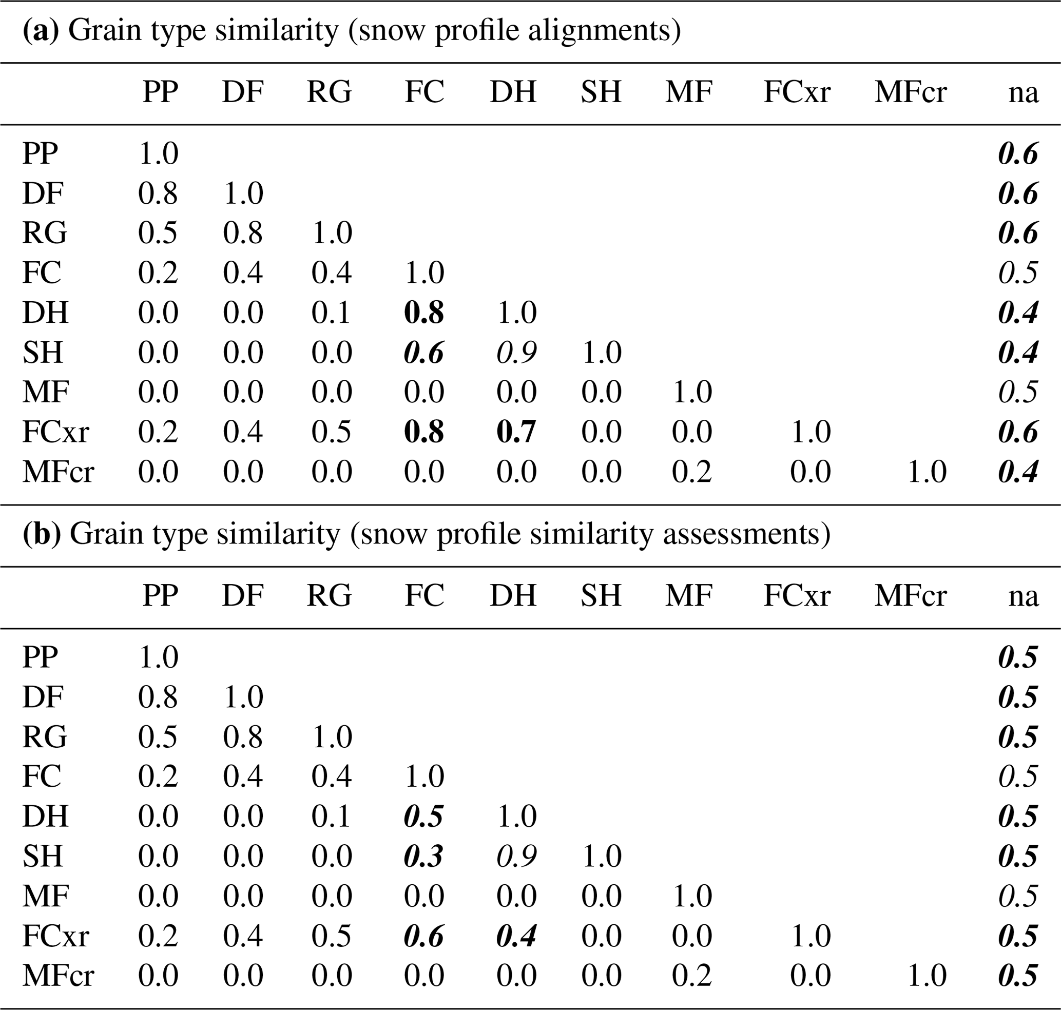
Since grain type is a categorical variable, calculating distances between nonidentical grain types is nontrivial. Our approach builds on the original method developed by Lehning et al. (2001), who defined a matrix of normalized grain type similarities between all possible pairs of grain types based on the physics of their formation and metamorphosis. Their approach evaluates the modeled grain type stratigraphy to identify model deficiencies and offer insight for model improvements. By contrast, our focus is on matching layers between snow profiles and assessing their similarity for avalanche hazard assessments. For the layer matching task, the similarity between grain types should indeed be evaluated partly based on their formation processes but also on the knowledge of snowpack model quirks and differences between modeled and observed profiles. For assessing the similarity of profiles, however, the similarity between grain types should be evaluated based on their implications for the hazard conditions rather than their formation processes. Thus, to make the approach more suitable for aligning snow profiles and assessing their similarity, we adapt the grain type similarity matrix of Lehning et al. (2001) for each of the two tasks separately (Table 1a, b). The matrices contain values within [0, 1] that represent the similarity between two grain types g₁ and g₂. Values >0.5 indicate similarity, 0.5 implies indifference, and values <0.5 indicate dissimilarity. The similarity between two grain types can be converted into a distance function d_g(g₁,g₂) by subtracting the similarity from 1 (i.e., the similarity between identical grain types is 1, and their distance is 0) to make it comparable to the other distance functions for hardness and layer date. Table 1a and b are modified from the grain type similarity matrix of Lehning et al. (2001) in the following ways (i.e., cells with italic font).

Table 1 Similarities between snow grain types as used for the layer alignment of snow profiles (a) and as used for the similarity assessment between snow profiles (b). Italic font represents modifications introduced by this publication, bold font highlights differences between the two tables (a) and (b), and all other values are taken directly from Lehning et al. (2001).

1. SH and DH layers are formed by very different processes – by the deposition of hoar onto the snow surface versus by kinetic growth of crystals within the snowpack. Consequently, Lehning et al. (2001) evaluated the similarity of the two grain types as completely dissimilar. However, both SH and DH represent hazardous weak layers and are of comparable importance in avalanche hazard assessments (Schweizer and Jamieson, 2001). Furthermore, practical experience with the current version of snowpack shows that SH layers are often converted to DH layers once buried. To account for both of these aspects, we raised their similarity from 0 to 0.9 for both tasks (Table 1a, b).

   Following the same line of logic, we also raised the similarity between SH and FC, another common weak layer grain type. However, to acknowledge the enhanced seriousness of buried SH layers while simultaneously facilitating the weak layer matching, the similarity between SH and FC is higher when aligning snow profiles (Table 1a) than when assessing their similarities (Table 1b)

2. Since human profiles sometimes lack grain type information for certain layers, an automated alignment algorithm needs to be able to cope with missing data in a meaningful way. Since it is more common for bulk layers to have missing grain type information, it is more desirable to match unknown grain types to bulk layers than weak layers. We therefore expanded the similarity matrix of Lehning et al. (2001) with an additional column for unknown grain types and filled it with values that are centered around indifference (i.e., 0.5) (Table 1b) but with a slight preference towards bulk layers (Table 1a).

3. While we acknowledge the physical similarity between DH, FC, and FCxr, we want to emphasize their slightly different implications for hazard conditions. We therefore classified DH layers – often representing buried SH layers or layers with large FC grains in simulated profiles – as first-order weak layers, whereas FC and FCxr were classified as second- and third-order weak layers, respectively. This hierarchy is implemented in Table 1b: similarities DH–FC and DH–FCxr are equal to and slightly lower than 0.5, respectively, and thus represent indifference or a slight mismatch; the similarity FC–FCxr is slightly greater than 0.5 and thus represents a weak match. These modifications lead to a pronounced distinction of the weak layer grains SH and DH from the less distinct weak layer grains FC and FCxr.

2.1.2 Distance function for layer hardness

The second important layer characteristic to consider is hardness, which characterizes the resistance of snow to penetration. In operational field observations the layer hardness is expressed on an ordinal hand hardness scale (Fierz et al., 2009). Hardness observations are taken by gently pushing different objects into snow layers from a snow pit wall. The hardness of a layer is expressed by the largest object that can be pushed into the snow layer with a consistent force of approximately 10–15 N. The ordinal levels of the hand hardness index are fist (F), four fingers (4F), one finger (1F), pencil (P), knife blade (K), and ice (I). Subclassifications like 4F+, 4F–1F, and 1F- are possible and refer to the descriptions “just harder than 4F”, “between 4F and 1F”, and “just softer than 1F”, respectively.

A translation of the ordinal index into a numerical scale is straightforward by assuming that “fist” equals a numerical value of 0, “ice” equals 6, and the ordinal levels are equidistant (Schweizer and Jamieson, 2007). The normalized distance d_h can then be written as $d_h(h_{\mathrm{1}},h_{\mathrm{2}})=\frac{|h_{\mathrm{1}}-h_{\mathrm{2}}|}{\mathrm{5}}$, where h₁ and h₂ represent numerical translations of two hand hardness values and the normalization factor of 5 refers to the largest distance possible (F–I). Hence, only layers with a hardness difference of fist to ice are considered completely dissimilar, while all other hardness combinations exhibit some degree of similarity.

2.1.3 Distance function for layer date

Snow layers are commonly labeled with either their deposition date (i.e., the date when a specific layer was formed) or their burial date (i.e., the date when a specific layer was buried). While snowpack models predominantly work with deposition dates, practitioners mainly use burial dates. One reason for practitioners’ preference for burial dates is the fact that layers can form over several days, which makes assigning a deposition date challenging. However, it is straightforward to derive the burial date of a simulated snowpack layer based on the deposition date of the overlying layer. Hence, layer dates of simulated snow profiles can easily be compared with layer dates recorded by practitioners.

The distance function d_t between two dates t₁ and t₂ becomes trivial as soon as the dates represent the same type of date (deposition or burial) and are converted into Julian dates: $d_t(t_{\mathrm{1}},t_{\mathrm{2}})=\frac{|t_{\mathrm{1}}-t_{\mathrm{2}}|}{c}$. In this case, the normalization factor c determines the time lag when the dates are considered to be completely dissimilar. A normalization factor of c=5, for example, means that date differences from 0 d to 4 d become increasingly dissimilar (i.e., $d_t\in [\mathrm{0},\mathrm{1}]$), whereas date differences equal to or greater than 5 d are considered completely dissimilar (i.e., d_t≥1; d_t typically does not exceed 2, but the exact limit depends on c and the length of the season or the size of the DTW window constraint). A normalization factor of c=1 means that only identical dates are considered to have any similarity. Hence, c can be used to account for small deviations in reported burial dates and in short time lags of weather patterns across geographic regions. In cases when layer dates are not available for one or both layers, the distance d_t defaults to indifference (i.e., d_t=0.5). This makes it possible to label only important layers with their date.

2.2 Aligning snow profiles with Dynamic Time Warping

In this section, we present a numerical algorithm that addresses the challenge of matching corresponding layers in snow profiles. Our method is based on Dynamic Time Warping (DTW), a long-standing algorithm, which was originally designed for speech recognition in the 1970s (Sakoe and Chiba, 1970; Sakoe, 1971; Sakoe and Chiba, 1978). Soon thereafter it was adopted in time series analyses (e.g., Berndt and Clifford, 1994), and it remains a state-of-the-art component in data-mining methods such as clustering and classification (e.g., Keogh and Ratanamahatana, 2005; Petitjean et al., 2011; Wang et al., 2013; Paparrizos and Gravano, 2015). Our discussion of DTW starts with a general background section, which is followed by four sections that explain our application of DTW to snow profiles in more detail. This includes snow profile preprocessing steps and inputs to the DTW algorithm. We then discuss suitable DTW parameter choices for snow profile alignments and make recommendations on how to use the alignment algorithm.

2.2.1 Background on Dynamic Time Warping

The following brief summary of DTW is based on Sakoe and Chiba (1978), Rabiner and Juang (1993), Keogh and Ratanamahatana (2005), and Giorgino (2009).

DTW is an elastic distance measure for time series or, more generally, sequences that calculates the dissimilarity between two sequences while allowing for distortions in “time”. The distortions are accommodated by mapping each element of one sequence to one or many elements of the other sequence (Fig. 1a). Once mapped, the dissimilarities between each of the matched sequence elements can be computed and combined into one single distance value that quantifies the dissimilarity between the two sequences.

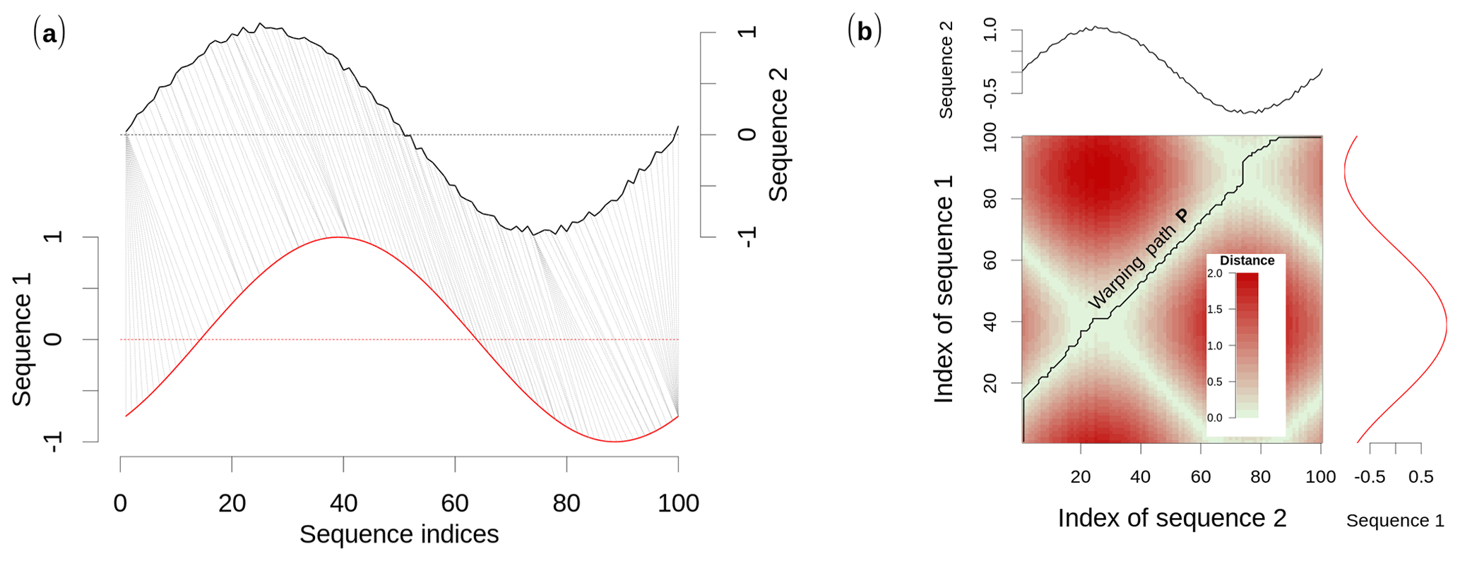
Figure 1 Illustrative example of the DTW alignment of two sine wave sequences. (a) Each element of the first sequence is mapped to one or many elements of the second sequence; the corresponding sequence elements can be found by (b) the (warping) path of least resistance through a local cost matrix that stores the distances between every possible pair of sequence elements.

To link corresponding sequence elements, a local cost matrix D is calculated that stores the distances between every possible pair of sequence elements. Hence, the dimensions of D are the lengths of the two sequences. Then, the best alignment of the two sequences is represented by the path of least resistance through D, which is referred to as the optimal warping path P (Fig. 1b). To ensure meaningful matching between sequence elements, the warping path is subject to the following constraints.

Monotonicity and continuity.

Subsequent elements of the warping path are contiguous in the sense that they are horizontally, vertically, or diagonally adjacent cells of the local cost matrix D, while “going back (in time)” is not allowed.

Warping window.

It is common practice to restrict the search for the optimal warping path to the bounds of a warping window around the main diagonal of the local cost matrix D. The main diagonal represents the lock-step alignment of the two sequences, whereby the ith element of the first sequence is mapped onto the ith element of the second sequence. Thus, the farther the warping path deviates from the main diagonal, the more extreme the warping gets, and sequence elements that are farther apart from each other are matched. The shape and size of the optimal warping window changes with the domain and the target data set. Popular choices include a slanted band of constant width (Sakoe–Chiba band) or a parallelogram between the sequences' start and end points (Itakura parallelogram). For detailed visualizations see Ratanamahatana and Keogh (2004). DTW with a constrained warping window is commonly referred to as constrained Dynamic Time Warping (cDTW).

Local slope constraint.

While the warping window constrains the envelope of the warping path globally, the so-called local slope constraint of the warping path ensures reasonable warping locally. More specifically, the local slope constraint controls how many subsequent elements of one sequence can be mapped onto one element of the other sequence. That is an important control because it regulates how much stretching and compressing of individual sequence elements is allowed. For time series, that means stretching and compressing with respect to time; in the case of snow profiles, it refers to the stretching and compressing of snow layer thicknesses.

Many different local slope constraints have been suggested in the literature. As an illustration, in Fig. 1, we use a nonrestrictive local slope constraint, which allows arbitrarily many elements to be mapped onto one corresponding element. In this case, the first element of Sequence 2 is mapped onto almost 20 elements of Sequence 1 (Fig. 1a), which requires a vertical start slope of the warping path (Fig. 1b). Find an explicit illustration of the nonrestrictive local slope constraint in Fig. B1a.

Boundary conditions.

For a global alignment, both the sequences' start and end points need to be elements of the warping path (Fig. 1b). Partial alignments can be computed by relaxing one or both of these constraints. This results in three different options: alignments for which the start but not the end points are matched (open-end alignment), alignments for which the end but not the start points are matched (open-begin alignment), or alignments for which subsequences of the two sequences that include neither the start or end points are matched. Further details on partial DTW matching can be found in Appendix A and in the review by Tormene et al. (2009).

Monotonicity and continuity.

Subsequent elements of the warping path are contiguous in the sense that they are horizontally, vertically, or diagonally adjacent cells of the local cost matrix D, while “going back (in time)” is not allowed.

Warping window.

It is common practice to restrict the search for the optimal warping path to the bounds of a warping window around the main diagonal of the local cost matrix D. The main diagonal represents the lock-step alignment of the two sequences, whereby the ith element of the first sequence is mapped onto the ith element of the second sequence. Thus, the farther the warping path deviates from the main diagonal, the more extreme the warping gets, and sequence elements that are farther apart from each other are matched. The shape and size of the optimal warping window changes with the domain and the target data set. Popular choices include a slanted band of constant width (Sakoe–Chiba band) or a parallelogram between the sequences' start and end points (Itakura parallelogram). For detailed visualizations see Ratanamahatana and Keogh (2004). DTW with a constrained warping window is commonly referred to as constrained Dynamic Time Warping (cDTW).

Local slope constraint.

While the warping window constrains the envelope of the warping path globally, the so-called local slope constraint of the warping path ensures reasonable warping locally. More specifically, the local slope constraint controls how many subsequent elements of one sequence can be mapped onto one element of the other sequence. That is an important control because it regulates how much stretching and compressing of individual sequence elements is allowed. For time series, that means stretching and compressing with respect to time; in the case of snow profiles, it refers to the stretching and compressing of snow layer thicknesses.

Many different local slope constraints have been suggested in the literature. As an illustration, in Fig. 1, we use a nonrestrictive local slope constraint, which allows arbitrarily many elements to be mapped onto one corresponding element. In this case, the first element of Sequence 2 is mapped onto almost 20 elements of Sequence 1 (Fig. 1a), which requires a vertical start slope of the warping path (Fig. 1b). Find an explicit illustration of the nonrestrictive local slope constraint in Fig. B1a.

Boundary conditions.

For a global alignment, both the sequences' start and end points need to be elements of the warping path (Fig. 1b). Partial alignments can be computed by relaxing one or both of these constraints. This results in three different options: alignments for which the start but not the end points are matched (open-end alignment), alignments for which the end but not the start points are matched (open-begin alignment), or alignments for which subsequences of the two sequences that include neither the start or end points are matched. Further details on partial DTW matching can be found in Appendix A and in the review by Tormene et al. (2009).

While there are many potential warping paths through the local cost matrix D that satisfy these constraints, the objective is to find the optimal warping path P that accumulates the least cost while stepping through D. This is an optimization problem that can be solved by dynamic programming. We refer the interested reader to Appendix A for more details.

2.2.2 Preprocessing of snow profiles: uniform scaling and resampling

The specific nature of snow profile data requires some preprocessing before DTW can be applied in a meaningful way. Variabilities in snowpack structures can be divided into systematic differences due to systematic variations in the meteorological forcing (e.g., location: a wind-scoured ridgeline next to a wind-loaded slope; elevation: increase in snowfall amounts with elevation) and random differences due to natural variations in the meteorological forcing (e.g., peculiar patterns of individual storms, small-scale variations) (Schweizer et al., 2007). The former can result in substantial differences in the snow profiles due to accumulation of different forcings over time. (See Sect. S1 in the Supplement for more details and visualizations of idealized stratigraphic snowpack variability.) While the DTW algorithm is well suited to deal with random differences, it was not designed to cope with systematic differences. Since systematic differences are common in snow profiles, it is necessary to preprocess them for a meaningful application of DTW. Fu et al. (2007) suggest uniform scaling, another optimization technique that minimizes systematic differences by determining an optimal global scaling factor. For efficiency reasons, we simply scale the snow profiles to identical snow heights instead. We thereby assume that the offset corresponds to approximately the magnitude of the systematic differences and that the rescaled profiles are predominantly characterized by random differences that can be handled by DTW. A tentative evaluation of this assumption can be found in the Supplement (Sect. S2.2).

Once the profiles have been rescaled, each of the two profiles consists of a series of discrete layers along an irregular height grid. To equalize the two different height grids, we resample the profiles onto a regular grid with a constant sampling rate, which represents the final resolution for the alignment procedure. While our algorithm allows users to flexibly set the sampling rate, a resolution of about half a centimeter ensures that typically thin, hazardous weak layers are being captured. Hence, the snow profiles included in the examples in this paper were resampled to 0.5 cm. To preserve the discrete layer character of each profile, we do not interpolate between the grid points during the resampling process.

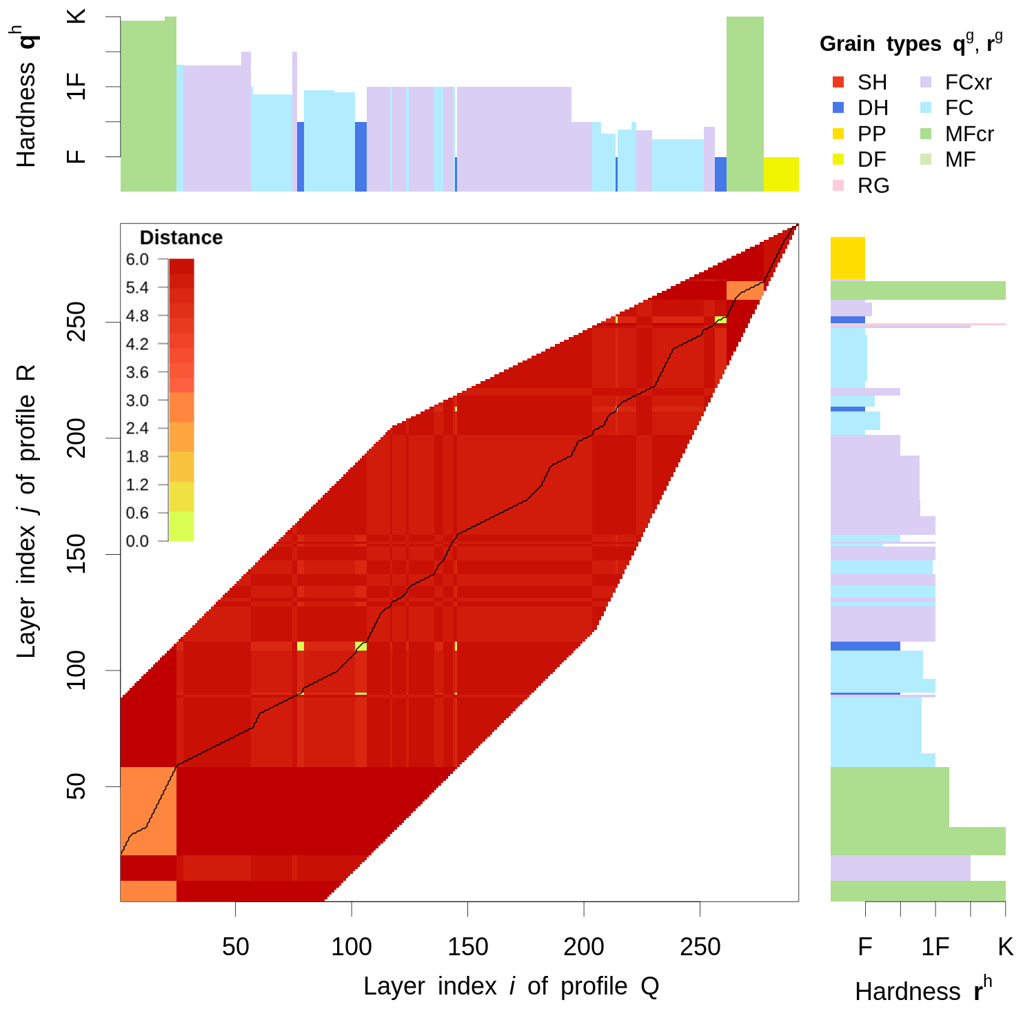
Figure 2 Visualization of a local cost matrix D, which stores the distance between individual layers of two snow profiles Q and R; Q and R contain the layer characteristics of grain type q^g and r^g, as well as hardness q^h and r^h. D is only filled with values around its diagonal; the rest is clipped by a warping window and a local slope constraint. The back line represents the optimal warping path P, which accumulates the least cost while stepping through D and which defines the alignment of the two profiles; the preferential layer matching implementation becomes apparent in the yellow and orange cells, which represent smaller than average distances and will thus be matched more easily. See the text for further explanation.

2.2.3 Computing a weighted local cost matrix from multiple layer characteristics

Section 2.2.1 introduced how DTW exploits the local cost matrix D to find the best alignment of two sequences. We will now show how to compute this local cost matrix for snow profiles. The following presentation therefore focuses on the layer characteristics of categorical grain type, ordinal layer hardness, and numerical layer date, which are the layer characteristics most commonly recorded by practitioners. Note, however, that the layer date contribution can be omitted if the information is not available, and our algorithm can easily be expanded to include other layer properties.

First, we combine the distances of the individual layer characteristics (defined in Sect. 2.1) into one scalar distance by weighted averaging. The resulting scalar distance fills one cell of the local cost matrix D and thus controls how the alignment algorithm matches the corresponding layers in the snow profiles.

Second, we use a weighting scheme for preferential layer matching (Fig. 2) to ensure that the algorithm prioritizes the alignment of snowpack features that are relevant for avalanche hazard assessment when calculating the scalar distance. The intent of the weighting scheme is to create anchor points for key layers by artificially introducing penalties for non-key layers. This is especially advantageous when no date information is available. Similar to our approach with the distance function for grain types, we focus on avalanche hazard assessment priorities and try to emulate a human alignment approach. First and second priority should be given to the alignment of first-order persistent weak layers (SH and DH) and crusts. Third priority should be given to the alignment of faceted grain types with first-order persistent weak layers. This cascade of priorities is expressed numerically by the relative differences of the weighting coefficients ν presented in Table 2. We determined these values experimentally by testing numerous snow profile alignments and found that they yield the wanted result without any unwanted side effects.

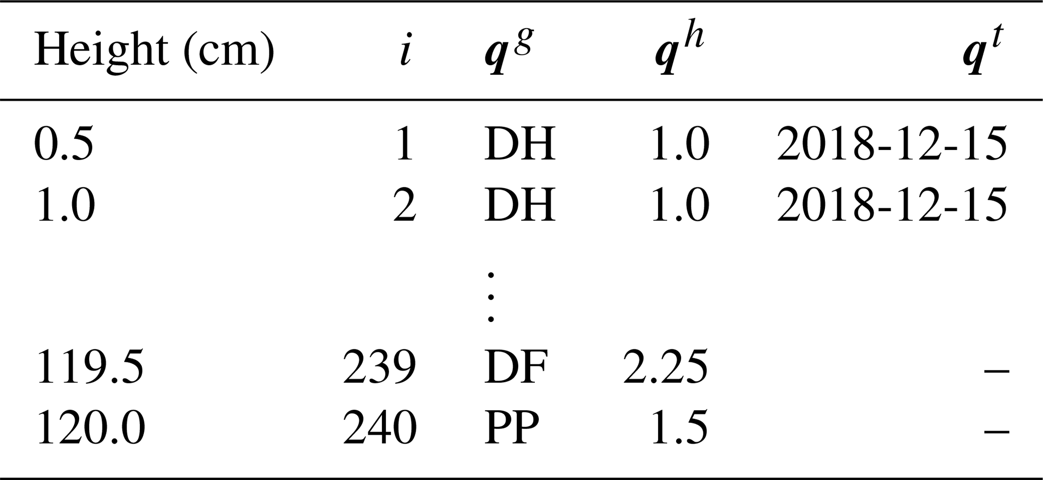
To compute D from two generic snow profiles, we introduce the following notation. Q and R are two rescaled and resampled snow profiles with I number of layers – typically on the order of hundreds of layers, depending on the sampling rate and the time of the season. The indices $i=\mathrm{1},\mathrm{\dots },I$ and $j=\mathrm{1},\mathrm{\dots },I$ refer to these layers. Each layer of the snow profiles Q and R contains information about the grain type, the hardness, the burial date, and the vertical position of the layer in the profile (i.e., height or depth). Those characteristics are denoted by q^g and r^g for grain type, q^h and r^h for hardness, and q^t and r^t for date (see Table 3 for an example). Each element D_ij of the local cost matrix D can then be written as

$$\begin{array}{}\text{(1)}& D_{ij}=w_g{d}_g(q_i^g,r_j^g)+w_h{d}_h(q_i^h,r_j^h)+w_t{d}_t(q_i^t,r_j^t)+\mathit{\nu }(q_i^g,r_j^g),\end{array}$$

where w_g, w_h, and w_t are averaging weights that sum up to 1 ($w_g+w_h+w_t=\mathrm{1}$). Those weights need to be estimated (see Supplement Sect. S2.1), but specific values are recommended in Sect. 2.2.5. Since d_g and d_h range within [0,1], d_t typically within [0,2], and ν within [0,5], the distance D_ij typically ranges within [0,7], where a distance of D_ij=0 refers to the two layers being identical. Note that in Eq. (1) d_g is calculated based on the similarity matrix in Table 1a, which is geared towards snow profile alignments. Figure 2 visualizes a local cost matrix derived from two generic snow profiles.

Table 2 Weighting scheme for preferential layer matching; the preferential layer matching coefficient ν(g₁,g₂) depends on the combination of two grain types g₁ and g₂; the smaller the coefficient, the more preferably the grain type combinations are matched (bold font). Values in the upper triangle are symmetric to values in the lower triangle.

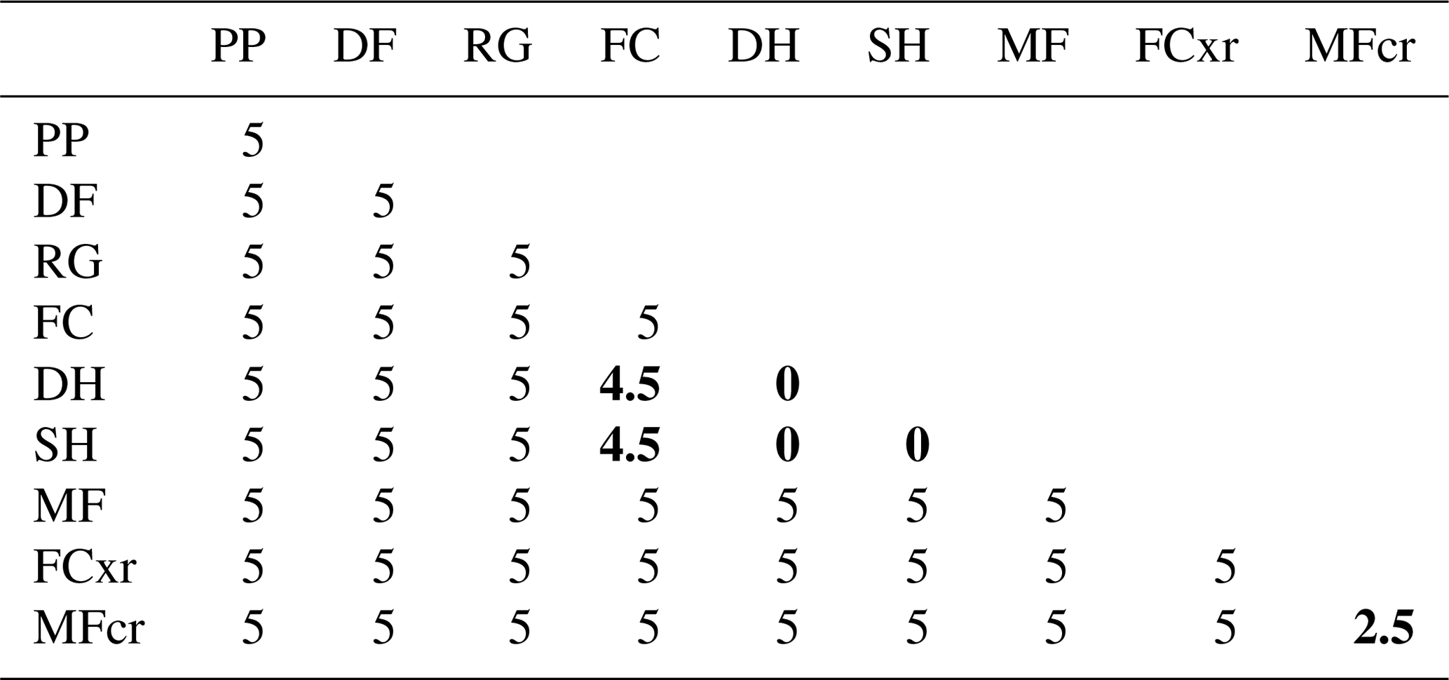
Table 3 An illustrative example of a resampled snow profile Q that contains information about the vertical position of the profile layers (at their top interfaces), the grain types q^g, the hardnesses q^h, and the (burial) dates q^t.

2.2.4 Obtaining the optimal alignment of the snow profiles

After calculating the local cost matrix D, there are several constraints on the warping path that need to be specified to tailor DTW to snow profile alignments; those constraints are the warping window, the local slope constraint, and the boundary conditions.

Warping window.

We use a slanted band of constant width around the main diagonal of D to constrain the warping path. This so-called Sakoe–Chiba band is quantified by the window size ε. See Sect. 2.2.5 for a recommendation on which value of ε to use for snow profile alignments.

Local slope constraint.

We require the local slope constraint to prevent excessive stretching or compressing of the snow layers in either of the two profiles. The symmetric Sakoe–Chiba local slope constraints (Sakoe and Chiba, 1978) do exactly that: they limit the amount of stretching or compressing to a specific factor, which is identical for both profiles. We chose a factor that limits the amount of stretching to double the layer thickness and the compression to half the layer thickness. On the technical level, that means that while stepping through D, a horizontal or vertical step is only allowed if following a diagonal step (Figs. A1, B1). The specific local slope constraint we refer to has been termed by Sakoe and Chiba (1978) as symmetric (P=1).

Note that the local slope constraint results in a funnel-shaped restriction of the warping window close to the starting point of the alignment, which is more restrictive than the slanted band window (Fig. 2). See Appendix A for a more detailed explanation.

Boundary conditions.

In cases when defining features of the snowpack at the very bottom or top only exist in one of the two profiles (e.g., lack of an early-season snowfall event or missing of the most recent storm at one of the two profile locations), partial snow profile alignments are more suitable than global alignments. In those situations the alignment benefits from relaxing the boundary conditions to accommodate those partial alignments (Figs. 2 and 3). We therefore implement symmetric open-end alignments, whereby an entire profile is mapped onto the other profile with the start points matched but the end points not.

Since open-begin alignments cannot be calculated with our chosen local slope constraint (Tormene et al., 2009), we developed a work-around by aligning snow profiles both bottom-up and top-down. The top-down alignment can be calculated straightforwardly by reversing both profiles and rerunning the DTW algorithm. However, since the DTW distance (Sect. 2.2.1, Appendix A) cannot be used to effectively identify the better alignment of the two, we use our independent, more nuanced similarity measure of snow profiles (addressed in Sect. 2.3) to assess the quality of the alignment.

Finding the optimal warping path P implies matching the corresponding layers between the two profiles Q and R. That in turn allows warping one profile onto the other one by optimally stretching and compressing its individual layer thicknesses so that the warped profile is optimally aligned with the other profile. For example, warping profile Q onto profile R produces the warped profile Q_w, which contains the same layer sequences as profile Q, but the adjusted layer thicknesses have aligned Q_w to the corresponding layers of R (Fig. 3). The optimally aligned profiles R and Q_w can now be used as input to an independent similarity measure.

2.2.5 Application cases and usage recommendations

There are two main application cases for the snow profile alignment algorithm: (i) aligning snow profiles from different locations (or sources) but at the same points in time and (ii) aligning snow profiles from the same location at different points in time.

Figure 3 The open-begin alignment of two snow profiles Q and R: the line segments match the corresponding layers between Q and R. Adjusting the layer thicknesses of profile Q yields the warped profile Q_w, which is optimally aligned to profile R.

In the first case, we recommend using open-end alignments when the optimal alignment of all individual layers is required – e.g., in applications that compare individual layers or in clustering applications that search for regions with similar snowpack conditions. We recommend using global alignments when modeled profiles are evaluated versus human profiles: even though open-end alignments might yield better alignment results, the explicit mismatch of layers at the very bottom or top of the profiles represents an important element of the model evaluation. Furthermore, keep in mind that open-end alignments increase the scope of the alignment algorithm, which can sometimes lead to surprising layer matches if the algorithm is used unsupervised.

In the second case, aligning profiles from the same location at different points in time (i.e., layer tracking), one of the two profiles typically has more layers and a higher snow depth. Since the smaller profile should be contained in the taller profile in a similar form, the alignment needs to be open-end and bottom-up. Furthermore, it is not necessary to rescale the profiles as recommended in Sect. 2.2.2 but only to resample them. In this case, rescaling actually moves corresponding layers farther apart, which would have to be compensated for by increasing the window size ε. To increase your control on which parts of the profiles are matched, we recommend that you label some of the key layers with their date information.

In the Supplement (Sect. S2), we derive the optimal values for the averaging weights w_g and w_h, as well as the window size ε, with a series of simulation experiments. Based on the results of these experiments, we recommend using the following default settings: ε≈0.3 in conjunction with a bottom-up/top-down approach² and a ratio of $w_h/w_g=\mathrm{1}/\mathrm{4}$. The value of w_d depends heavily on how similar the meteorological processes are that shape the snowpack at the two locations; e.g., two profiles from the same elevation and the same aspect that are in close proximity can be aligned based on layer date alone. However, two profiles from opposite aspects and different elevation bands may be aligned predominantly based on grain type and hardness.

2.3 Assessing the similarity of snow profiles

A measure that quantifies the similarity of snow profiles as a whole is best designed independently from a profile alignment or layer matching routine. Such an independent approach allows for matching layers based on physical similarity (i.e., processes like grain formation and metamorphism or knowledge about snow cover models), whereas the similarity of the aligned profiles can be assessed based on characteristics relevant for avalanche hazard assessment. Therefore, we define a similarity measure Φ for generic snow profiles based on the layer characteristics of grain type and hardness, which can be used to numerically compare, evaluate, and group snow profiles.

Let us again consider two snow profiles. Some of their layers have been matched, while others have not. The non-matched layers are located either at the very bottom or very top of one of the two profiles. For example, the two profiles could be the profiles R and Q_w from the previous section. Our goal is to compute a scalar number that expresses the similarity between these two profiles on a scale from 0–1. To do so, we start again by computing the (dis)similarities between the corresponding layers analogously to the previous sections. However, in a similarity measure that is geared towards hazard assessment not every layer is equally important. Furthermore, since important weak layers are often much thinner than the bulk layers, they would be dramatically underrepresented in a measure that computes a standard average across all layers. Thus, we bin all layers according to four major grain type classes relevant for avalanche hazard assessments: (1) new snow crystals (PP and DF) that are commonly associated with surface problems, (2) weak layers (SH and DH) and (3) crusts (MFcr) that are typically related to persistent avalanche problems, and (4) all other grain types that represent bulk layers. We calculate separate similarity values for every class (a scalar value within [0, 1]), and the overall similarity between the two profiles is the average similarity derived from the classes.

To calculate the similarity for a grain type class, we first distinguish between matched and non-matched layers. All non-matched layers are treated as indifferent and are therefore assigned a similarity value of 0.5. Such a strategy makes the measure robust against a varying number of non-matched layers. Next, we calculate the similarities of all matched layers. That can be done with the distance functions from Sect. 2.1, which compute the dissimilarity between two layers based on grain type or hardness. Note that in this context, the grain type distance is calculated based on Table 1b to ensure that the derived similarity is most useful for avalanche forecasting. The resulting distance is converted into a similarity by subtracting the distance from 1 (i.e., a distance of 0.8 becomes a similarity of 0.2). If the grain type class is new snow crystals or bulk grains, the similarity of a matched layer is computed as the product of the associated similarity of grain type and hardness. The emerging similarity for the entire class is then the average over all (matched and non-matched) layers within.

While the above approach works well for new snow crystals and bulk layers, weak layers and crusts require additional considerations to be integrated in a meaningful way.

First, given weak layers or crusts, an identical match of the grain type is arguably more important than a hardness evaluation: many weak layers and crusts are thin, and often melt–freeze crust laminates are characterized by an inhomogeneous hardness. These circumstances challenge precise hardness measurements of these layers and make them prone to error. Additionally, crusts play an important role in avalanches not as a weak layer themselves, but as a layer favoring adjacent weak layer growth (Jamieson, 2006). That in turn makes the grain type of a crust much more important than its hardness when evaluating the similarity between two layers. In summary, a hardness evaluation might introduce more error than benefit, especially when comparing human versus modeled profiles. Therefore, we compute the similarity of a matched weak layer or crust as the associated similarity of grain type alone, thereby neglecting hardness information.

Second, for weak layers and crusts, it is specifically important where in the profile they are located. Consider a snow profile with two DH layers close to the ground and one SH layer buried under new snow. A second, almost identical profile lacks the buried SH layer. While the likelihood of triggering and the potential size of avalanches are similar with respect to the two matched DH layers, they are not with respect to the buried SH layer, which is missing in the second profile. Even though the two profiles are visually almost identical, they require different avalanche risk management approaches. If we calculated the similarity for the weak layer class of those two profiles as described above (i.e., as an average over all layers), the thin SH layer would be heavily underrepresented among the thicker DH layers. As a consequence, the weak layer class would exhibit a high similarity value. For example, if the two DH layers were each 10 cm thick, the SH layer 2 cm, and the sampling rate were 1 cm, then the similarity for the weak layer class would be $(\mathrm{20}\cdot \mathrm{1}+\mathrm{2}\cdot \mathrm{0})/\mathrm{22}=\mathrm{0.9}$. Given that the two snowpack conditions demand different risk management approaches, such a high similarity is not meaningful. To mitigate those situations, we divide the two profiles into sections of equal thickness and evaluate the similarity of the weak layers and crusts within those sections separately. The number of sections is determined by the maximum number of weak layers (or crusts) in either of the two profiles. By evaluating similarities of adjacent weak layers or crusts, we introduce a basic weighting scheme for the position of those layers in the profile. It is based on the idea that avalanche likelihood and size, as well as resulting risk management, are rather similar for adjacent weak layers or crusts but rather different for weak layers or crusts in opposing depths of the profile. In our example, there are three weak layers; hence, the two profiles are divided into three sections of equal thickness. We assume that all weak layers that are in the same section require a similar risk management approach. So, the similarity for each section is the average similarity of the weak layers within, and each section is equally important for the hazard assessment, so the similarity for the weak layer class is the average similarity with respect to the sections. In our example, the lower section contains the two DH layers, the middle section contains no weak layers, and the upper section contains the SH layer in one profile. Hence, the similarity for the weak layer class is $\left(\frac{\mathrm{20}\cdot \mathrm{1}}{\mathrm{20}}+\frac{\mathrm{2}\cdot \mathrm{0}}{\mathrm{2}}\right)/\mathrm{2}=\mathrm{0.5}$. A weak layer similarity of 0.5 represents the two snowpack conditions much better than a similarity of 0.9.

In summary, the resulting similarity measure Φ between two snow profiles expresses the similarity between these two profiles in a scalar value within [0, 1]. A similarity of 1 corresponds to the two profiles being identical. Note that the measure is symmetric to the two profiles so that the first profile is as similar to the second profile as the second is to the first. By treating non-matched layers as indifferent the measure is able to cope with varying numbers of missing layers at the bottom or top of the profiles, which is important for assessing the similarity of snow profiles from different times and/or locations. To make the similarity measure useful for avalanche forecasting, it weighs hazardous thin layers, crusts and storm snow layers more heavily than bulk layers, and it considers the relative depth of those layers.

3 Aggregation and clustering applications – a practical valuation

Section 2.2 and 2.3 detail how to match layers between snow profiles and how to assess the similarity of the aligned profiles for applications in avalanche hazard assessment. Both of these steps are fundamental prerequisites to automate forecaster tasks, such as grouping similar profiles and finding the representative profile of a group. In the data sciences, these tasks are called data clustering and data aggregation. In this section, we demonstrate how to apply simple data clustering and data aggregation methods to snow profiles based on their prior alignment and similarity assessment. We use these application examples as a face validation of our methods.

3.1 Clustering of snow profiles

Avalanche professionals need to group snow profiles to understand how snowpack conditions and avalanche hazard vary across space. The snow profile alignment algorithm and similarity measure described in the previous section enable the automation of this task by providing the necessary quantitative link to the well-established field of numerical clustering methods (e.g., James et al., 2013; Sarda-Espinosa, 2019).

To showcase the clustering of snow profiles based on our similarity measure, we use a set of 12 snow profiles that exhibit both pronounced and subtle differences in their snowpack features (Fig. 4). The alignment and similarity assessment of the snow profiles is based on grain type and hardness information, even though they are visualized in Fig. 4 solely by their grain type sequences. After computing a total of $\mathrm{12}\cdot \mathrm{11}=\mathrm{132}$ profile alignments and similarity assessments, the clustering is carried out by an agglomerative hierarchical clustering algorithm that iteratively fuses individual profiles to clusters based on the similarity of the profiles³. The resulting cluster hierarchy is best analyzed from the top to the bottom, allowing us to separate the set of 12 profiles into up to 12 clusters. The higher a split occurs in the hierarchy, the more distinct the corresponding clusters are from each other.

Figure 4 Hierarchical clustering of 12 snow profiles based on prior snow profile alignment and similarity assessment. The colors represent the grain types of distinct layers, and the bold black lines separate the four most distinct clusters.

The first most distinct split separates the heavily faceted profiles 1–4 from the remaining profiles. The remaining profiles are generally quite similar, except for some subtle but important features that still require different risk management strategies: profiles 5–7 show weak layers in the middle of the snowpack and below the new snow (i.e., second split); profiles 8 and 9 have a weak layer sandwiched between two crusts at the bottom of the snowpack (i.e., third split), and profiles 10–12 either have a weak layer only in the middle of the snowpack or none at all. Additionally to examining those most distinct four clusters, the similarities within the clusters can be investigated further. For example, profile 1 is the most dissimilar profile within the first cluster, being the only profile with a crust below the new snow and the only profile with a pronounced weak layer in mid-snow height. As another example, profile 10 is the outsider in cluster 4, having no weak layer at all.

The relationships among the profiles as established by the alignment algorithm and similarity measure yield a sound clustering result that looks similar to how a human avalanche forecaster would group the profiles according to different strategies on how to manage snowpack conditions and the related avalanche hazard. This example demonstrates that our approach can differentiate between very different and subtly different snowpack conditions.

3.2 Finding a representative snow profile: the medoid

Avalanche forecasters often draw a representative snow profile that summarizes the most important snowpack features within a group of profiles. In the data-mining community, this type of generalization is typically called the average sequence, or aggregate, and the most sophisticated methods for computing that aggregate are closely tied to the alignment algorithm and similarity measure used (e.g., Petitjean et al., 2011; Paparrizos and Gravano, 2015). In the following, we use the simple approach of identifying the one profile within the group that is most similar to all other profiles, called the medoid profile. Visually, the medoid profile can be thought of as the member of the group that is closest to the geometric center of the group. Mathematically, that means that the medoid profile minimizes the accumulated distances to all other profiles. To identify the medoid, we compute the accumulated distances to all other profiles for every profile. As the distance δ between two profiles Q and R we use the similarity measure Φ after converting it to a distance by subtracting it from 1 (see Sect. 2.3). We apply the similarity measure to both profile pairs (Q, R_w) and (Q_w, R) to account for missing layers. Hence,

$$\begin{array}{}\text{(2)}& \mathit{\delta }(Q,R)=max\mathit{\{}\mathrm{1}-\mathrm{\Phi }(Q,R_{\text{w}}),\mathrm{1}-\mathrm{\Phi }(Q_{\text{w}},R\left)\mathit{\right\}}.\end{array}$$

The pairwise distances between the profiles of the group can be translated into a configuration plot, which gathers similar profiles close to each other and dissimilar ones further away from each other⁴ (Fig. 5). The medoid profile, being most similar to all other profiles, is the member of the group that represents the group the best. We use the same set of 12 profiles as in Sect. 3.1 to demonstrate the profile aggregation. As the snowpack conditions within the set are too different to meaningfully represent them by one representative profile (Fig. 5a), we can combine clustering and aggregating to draw the representative profiles of the most distinct clusters within the set (Fig. 5b – the three clusters consist of profiles 1–4, 5–7, and 8–12, as depicted in Fig. 4).

While our proof of concept demonstrates a sound and reliable workflow, using the medoid profile may be computationally too expensive to efficiently deal with data volumes beyond the order of tens to hundreds of profiles on an operational basis. However, Paparrizos and Gravano (2015) show that the medoid approach performs slightly better than any other sequence aggregation method. Dynamic Time Warping Barycenter Averaging (Petitjean et al., 2011) might be an alternative aggregating method that could be evaluated in future studies.

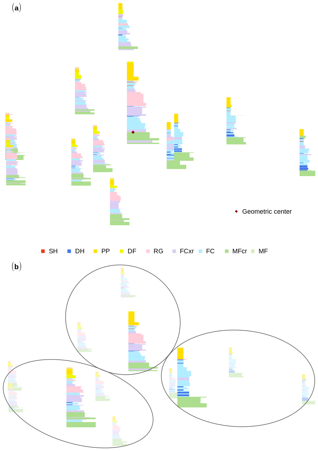
Figure 5 Configuration plots of a group of 12 snow profiles with similar profiles gathered close to each other. (a) The geometric center of the whole group, which identifies the most representative profile. (b) The three most distinct subsets of the whole group, highlighting their associated representative profiles; see Fig. 4.

4 Discussion and conclusions

The snow profile alignment algorithm and the similarity measure presented in this paper aim to address two of the main factors that have limited the adoption of snowpack models to support avalanche warning services and practitioners. First, the methods provide the foundation for numerical grouping and summarizing snow profile data and can thus help to make snowpack model output more accessible by addressing any avalanche operation fundamental questions: where in the terrain do we find which conditions? Second, our methods have the potential to make snowpack models more relevant to avalanche forecasters by providing a means for model evaluation against human observations.

Building on the well-established and long-standing concept of Dynamic Time Warping (DTW), we developed a snow profile alignment algorithm that combines multiple layer characteristics of categorical, numerical, and ordinal format into a weighted metric and feeds into existing DTW algorithms such as the open-source R package dtw (https://dynamictimewarping.github.io/, last access: 7 January 2021) (Giorgino, 2009). Moreover, we reviewed and derived useful DTW configurations and hyper-parameter settings for snow profile applications. Since these applications rely on operationally available profile observations that typically focus on information relevant for current avalanche conditions only, our approach is able to handle missing data and take advantage of select layer date tags. To maximize the layer matching performance for profiles with limited details, we implemented a scheme for preferential layer matching based on domain knowledge. In parallel, Viallon-Galinier et al. (2020) extended the layer matching algorithm from Hagenmuller and Pilloix (2016) to conduct a detailed, process-related evaluation of the snowpack model Crocus based on high-quality snow profile observations with a large variety of observed variables that are sampled at specific study sites at regular intervals. Since their goal is the correction of deviating model states with a direct insertion assimilation scheme based on point-scale simulations and observations, their evaluation targets not only each individual layer, but also each individual layer characteristic separately. To address operational avalanche forecasting needs, we additionally developed a similarity measure that focuses on avalanche-forecasting-specific considerations for which certain layers are considered more important. Moreover, combining information from individual layers and their characteristics into a scalar measure allows for clustering and aggregating sets of profiles to characterize and evaluate the regional-scale avalanche hazard conditions.

In the data-mining community, similarity (or distance) measures are evaluated through classification applications (Wang et al., 2013). Since snow profile data sets that represent the ground truth of alignments or groupings do not (yet) exist, the evaluation of our methods needs to rely on expert judgment or application valuation. During the development of our algorithm, we therefore manually evaluated the alignment of many profile pairs, a few of which are shown in Sect. S3 of the Supplement to demonstrate its behavior. Furthermore, we evaluated the interplay of the alignment algorithm and similarity measure through clustering and aggregation applications. Those applications involve many individual profile assessments and therefore represent a meaningful valuation approach, which shows that the alignment algorithm and similarity measure are capable of distinguishing between subtle differences in the snow stratigraphy and yield a sound grouping that could have been carried out by a human avalanche professional.

Although our methods have been designed to accommodate a wide range of requirements and to cope with a variety of scenarios, the following limitations should be considered. First, while the layer matching algorithm can easily be applied to large data sets in an unsupervised manner, not all scenarios within such a data set might be best served with the same parameter settings. Getting meaningful results in highly diverse data sets requires the algorithm to be less constrained. However, this can also result in unrealistic alignments. Second, when alignments are based on grain type and hardness alone, the matching of layers can sometimes be ambiguous – even for human experts. In those cases, labeling a few key layers with their burial date can greatly improve the alignment accuracy with little extra effort, especially as the labeling of weak layers is already established practice in North America (Canadian Avalanche Association, 2016). Note that our algorithm can easily be expanded to include other layer properties, especially if they are of ordinal or numeric data types such as grain size or specific surface area. Third, it is important to recognize that any numerical approach that condenses the complexity of these similarity assessments to a one-dimensional scale within [0, 1] is unable to capture the full expertise and situational flexibility of human forecasters. However, it is a critical prerequisite for algorithmically grouping profiles and establishing ranks among them. As such our similarity measure offers a consistent evaluation of snow profiles that is based on the most commonly available layer characteristics. And lastly, the similarity measure and consequently the clustering and aggregating applications are purely based on the agreement of the snowpack structure. Hence, snow depth is not a driver of our similarity assessment unless it leads to deviations in the snow stratigraphy. If combined with monitoring of the snow depth distribution, a clustering or aggregation application can provide a comprehensive picture of the conditions within a specific forecast area.

Since our methods aim to help overcome the operational challenges of summarizing snowpack model data and evaluating that data, we imagine its integration into operational avalanche forecasting as follows. Traditionally, an avalanche risk management operation, such as a public warning service or a backcountry guiding operation, obtains vital information about the snowpack through manual snow pit observations at select point locations. Simulated snow profiles across a mountain drainage can sample the snowpack conditions similarly to field observations, except with higher spatiotemporal coverage and independent from external circumstances. Our methods could group the simulated profiles according to similar conditions, potentially uncovering different avalanche problems. Furthermore, that grouping could quantify the prevalence of those conditions, and the conditions could be linked to their specific location, elevation, and aspect. Then, the different conditions could be summarized by their representative profile to present the data in a familiar way. Human forecasters can then use that simulated data as an additional data source complementing the field observations or deploy targeted field observations to verify the model output. Through a continuous evaluation of the model output against human observations or human assessments (e.g., synthesized snow profiles), the current validity of the simulations could potentially be extrapolated into data-sparse regions. More generally, a continuous evaluation of operational snowpack simulations provides an opportunity to better understand the strengths and weaknesses of the involved model chain for its application in avalanche forecasting. Through this line of research, we hope that snowpack models will be further incorporated into operational avalanche hazard assessment routines so that avalanche forecasters can begin to build an understanding of how to interpret and trust snowpack simulations.

Appendix A: An exemplary solution to the DTW optimization problem

In this section we explain the concept of solving the DTW optimization problem and thereby finding the optimal warping path P through the local cost matrix D. We do this by applying some of the same constraints that we also use in the snow profile alignment algorithm, most notably the Sakoe–Chiba local slope constraint (symmetric, P=1; Fig. B1b) and (symmetric) open-end boundary conditions (see Sect. 2.2.4).

As mentioned in Sect. 2.2.1, the DTW optimization problem can be solved recursively with the aid of dynamic programming. Imagine a local cost matrix D (i by j) with individual elements D_ij. Another, yet empty, matrix G – the accumulated cost matrix – has the same dimension as D. From the boundary conditions, we know that the first items of the two sequences need to be matched. Thus, the optimal warping path P starts at G₁₁, which holds the same value as D₁₁. From the local slope constraint, we know that a horizontal or vertical step is only allowed if following a diagonal step. Therefore, as we are about to do our first step, we have to do a diagonal one to G₂₂. G₂₂ is the second element of the optimal warping path P, and its value can be calculated by the accumulated cost one step before (i.e., G₁₁) plus twice the local cost of the current step (i.e., D₂₂); hence, $G_{\mathrm{22}}=G_{\mathrm{11}}+\mathrm{2}{D}_{\mathrm{22}}$ (where the weighting factor 2 represents a slope weight; see Appendix B). Since we just did a diagonal step, we are now allowed to step up vertically, diagonally, or horizontally to fields G₂₃, G₃₃, or G₃₂, respectively.

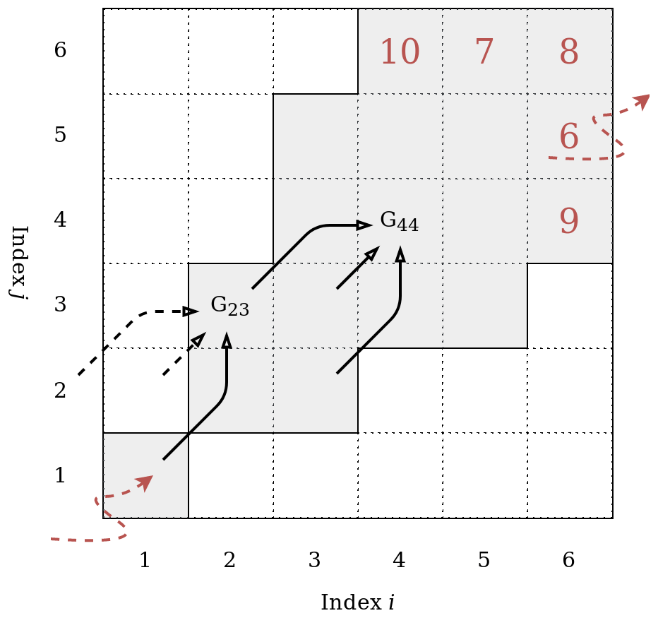
Figure A1 Sketch of a cost matrix G that stores the smallest accumulated cost of visiting a matrix element G_ij. In an open-end alignment, the optimal warping path P starts at G₁₁. The steps of the warping path are governed by the chosen local slope constraint (black arrows) such that only the grey matrix cells can be visited. The warping path ends in the last row or column of the matrix wherein the accumulated cost is smallest (i.e., at G₆₅=6). See the text for more details.

More generally, any element G_ij can be calculated by the recursion

$$\begin{array}{}\text{(A1)}& G_{ij}=min\left[\begin{array}{l}{G}_{i-\mathrm{1}j-\mathrm{2}}+\mathrm{2}{D}_{ij-\mathrm{1}}+D_{ij}\\ G_{i-\mathrm{1}j-\mathrm{1}}+\mathrm{2}{D}_{ij}\\ G_{i-\mathrm{2}j-\mathrm{1}}+\mathrm{2}{D}_{i-\mathrm{1}j}+D_{ij}\end{array}\right].\end{array}$$

Figure A1 sketches that concept. Each individual step of the optimal warping path P is governed by the local slope constraint such that only a limited number of matrix elements can be visited by the warping path. Each of those elements of the cost matrix G in turn stores the smallest accumulated cost that is necessary to arrive at that cell. In a symmetric open-end alignment, the final element of the optimal warping path P is the one element in the last column or row of G that has accumulated the least cost.

If the optimal warping path P has K elements from $k=\mathrm{1},\mathrm{\dots },K$, then each element p_k stores its location in the cost matrix by ${\mathit{p}}_k=(p_k^i,p_k^j)$. Consequently, the accumulated cost of the optimal warping path P can be expressed as $G_{p_K^i{p}_K^j}$. For example, for the warping path implied by Fig. A1, $\mathit{P}=\mathit{\left\{}\right(\mathrm{1},\mathrm{1}),(\mathrm{2},\mathrm{2}),\mathrm{\dots },(\mathrm{6},\mathrm{5}\left)\mathit{\right\}}$ and $G_{p_K^i{p}_K^j}={\text{G}}_{\mathrm{65}}=\mathrm{6}$. Finally, the DTW distance between two sequences, d_DTW, is expressed by the accumulated cost of the optimal warping path P normalized by the length of the path (expressed as Manhattan distance from the matrix origin, for symmetric recursions), i.e.,

$$\begin{array}{}\text{(A2)}& d{}_{\text{DTW}}={\displaystyle \frac{\mathrm{1}}{p_K^i+p_K^j}}{G}_{p_K^i{p}_K^j}.\end{array}$$

In Sect. 2.2.4 we introduced the warped snow profile Q_w. With the insight gained from the current section, we can now precisely define the warped profile Q_w. Therefore, we adopt the notation introduced in Sect. 2.2.3 and additionally denote the layer height of the snow profiles Q_w and R as ${\mathit{q}}_{\text{w}}^{\text{Ht}}$ and r^Ht, respectively. Then the warped profile Q_w can be constructed with the indices pⁱ and p^j, which are given by the warping path P by

$$\begin{array}{}\text{(A3)}& {\displaystyle }{\mathit{q}}_{\text{w}}^{\text{Ht}}& {\displaystyle }={\mathit{r}}_{{\mathit{p}}^j}^{\text{Ht}},\text{(A4)}& {\displaystyle }{\mathit{q}}_{\text{w}}^g& {\displaystyle }={\mathit{q}}_{{\mathit{p}}^i}^g.\end{array}$$

The vectors ${\mathit{q}}_{\text{w}}^h$ and ${\mathit{q}}_{\text{w}}^t$ can be calculated analogously to Eq. (A4).

Appendix B: Exemplary DTW step patterns

DTW step patterns describe the local slope constraint and the slope weights associated with each step of the warping path. While the local slope constraint limits the warping path to physically meaningful steps, the slope weights, which depend on the local indices' increments, ensure that different alignments can be compared. Both step patterns used in this paper use slope weights that are symmetric to the query and reference sequences but asymmetric slope weights that favor the advance of a certain sequence also exist (Rabiner and Juang, 1993; Sakoe and Chiba, 1978; Giorgino, 2009).

While the symmetric, unconstrained step pattern allows the warping path to advance diagonally, vertically, or horizontally at any time of the alignment (Fig. B1a, used in the alignment of sine waves shown in Fig. 1), the Sakoe–Chiba symmetric (P=1) step pattern enforces a diagonal step preceding each horizontal or vertical step to limit the stretching and compressing of the sequences to a factor of 2 and 1∕2, respectively (Fig. B1b, used for snow profile alignments as in Figs. 2, 3).

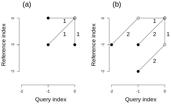
Figure B1 Two exemplary DTW step patterns that illustrate different symmetric local slope constraints and their associated slope weights. While panel (a) shows an unconstrained pattern, panel (b) shows a pattern that limits the stretching of either sequence to a factor of 2 by enforcing a diagonal step before a horizontal or vertical one.