Comparison of ocean vertical mixing schemes in the Max Planck Institute Earth System Model (MPI-ESM1.2)

For the first time, we compare the effects of four different ocean vertical mixing schemes on the mean state of the ocean and atmosphere in the Max Planck Institute Earth System Model (MPI-ESM1.2). These four schemes are namely the default Pacanowski and Philander (1981) (PP) scheme, the K-profile parameterization (KPP) from the Community Vertical Mixing (CVMix) library, a recently implemented scheme based on turbulent kinetic energy (TKE), and a recently developed prognostic scheme for internal wave dissipation, energy, and mixing (IDEMIX) to replace the often assumed constant background diffusivity in the ocean interior. In this study, the IDEMIX scheme is combined with the TKE scheme (collectively called the TKE+IDEMIX scheme) to provide an energetically more consistent framework for mixing, as it does not rely on the unwanted effect of creating spurious energy for mixing. Energetic consistency can have implications on the climate. Therefore, we focus on the effects of TKE+IDEMIX on the climate mean state and compare them with the first three schemes that are commonly used in other models but are not energetically consistent.

We find warmer sea surface temperatures (SSTs) in the North Atlantic and Nordic Seas using KPP or TKE(+IDEMIX), which is related to 10 % higher overflows that cause a stronger and deeper upper cell of the Atlantic meridional overturning circulation (AMOC) and thereby an enhanced northward heat transport and higher inflow of warm and saline water from the Indian Ocean into the South Atlantic. Saltier subpolar North Atlantic and Nordic Seas lead to increased deep convection and thus to the increased overflows. Due to the warmer SSTs, the extratropics of the Northern Hemisphere become warmer with TKE(+IDEMIX), weakening the meridional gradient and thus the jet stream. With KPP, the tropics and the Southern Hemisphere also become warmer without weakening the jet stream. Using an energetically more consistent scheme (TKE+IDEMIX) produces a more heterogeneous and realistic pattern of vertical eddy diffusivity, with lower diffusivities in deep and flat-bottom basins and elevated turbulence over rough topography. IDEMIX improves in particular the diffusivity in the Arctic Ocean and reduces the warm bias in the Atlantic Water layer. We conclude that although shortcomings due to model resolution determine the global-scale bias pattern, the choice of the vertical mixing scheme may play an important role for regional biases.

1 Introduction

Vertical mixing in the ocean is a complex phenomenon and its magnitude depends on processes acting over a large range of vertical and horizontal scales, from about 1 km to several metres down to centimetres (Fox-Kemper et al., 2019). Vertical mixing affects key elements in the ocean that are of climatic importance, such as ocean stratification, the distribution of temperature, salinity and passive tracers, the ocean uptake of heat and carbon, and the global meridional overturning circulation (MOC; e.g. Gent, 2018).

In ocean models, the processes that lead to mixing are subgrid scale and therefore not resolved, so they have to be parameterized. The complexity of these parameterizations varies in dependence of our understanding, application, and available resources (e.g. Large et al., 1994; Fox-Kemper et al., 2019). In fact, the parameterization of vertical mixing constitutes one of the current shortcomings of ocean models (Robertson and Dong, 2019; Fox-Kemper et al., 2019).

Frequently used ocean vertical mixing schemes date back to the 1980s and 1990s. Often, a modelling centre or a group decides to implement only one of these schemes and, for practical reasons such as tuning effort, not to deviate from it afterwards. However, as these schemes are based on different principles, deviations in the results are to be expected. We further note that even the same scheme may produce different results due to the numerical implementation (e.g. Li et al., 2019) and small modifications (e.g. Danabasoglu et al., 2006).

In the ocean surface boundary layer, schemes diagnose vertical profiles of scalar mixing diffusivity and viscosity from surface forcing and background fields, such as in the Pacanowski and Philander (1981) (PP) scheme or in the K-profile parameterization (KPP; Large et al., 1994). Second-order schemes (Mellor and Yamada, 1982), such as the turbulent kinetic energy (TKE) scheme (Gaspar et al., 1990), contain in addition to the mean quantities also prediction equations for higher-order moments, i.e. for variance and covariance terms of heat and momentum. These two most common approaches represent processes that result in vertical shear of the velocity and in changes of the buoyancy, e.g. due to convection. These schemes can become more complex by adding further subgrid-scale processes (Fox-Kemper et al., 2019), such as mixing by Langmuir turbulence (e.g. McWilliams et al., 1997; Li and Fox-Kemper, 2017; Li et al., 2019) or internal tides (Garrett, 2003). Although KPP is probably the most widely used scheme in ocean models, TKE is also a frequent choice and is part of state-of-the-art ocean models and for which also extensions such as Langmuir turbulence (Axell, 2002) or surface waves (Breivik et al., 2015) were developed.

For the first time, we compare four ocean vertical mixing schemes side by side in a coupled climate model, that is, the Max Planck Institute Earth System Model (MPI-ESM1.2). The traditional schemes (PP, KPP, TKE) all artificially create energy for mixing, which is introduced by the arbitrary background diffusivity. However, this spurious energy source is an unwanted effect in an ocean model. We therefore implement a prognostic scheme for internal wave energy in the ocean, termed internal wave dissipation, energy, and mixing (IDEMIX; Olbers and Eden, 2013). IDEMIX is a natural extension to TKE, as it is also based on an energy budget equation that is linked with TKE by the dissipation of internal wave energy. This prognostic dissipation term replaces the otherwise artificial background diffusivity. Together, the TKE+IDEMIX scheme theoretically provides an energetically more consistent scheme for vertical mixing in the ocean. The practical effect of IDEMIX on the climate state, however, has hardly been studied, with the exception of the work of Nielsen et al. (2018).

The four schemes, whose effect on the climate state we investigate, are the default PP scheme from MPI-ESM1.2, KPP, TKE, and TKE+IDEMIX (see Sect. 2.1 and Appendix A for details). Note that we do not break down the effects found to the process level for which idealized uncoupled ocean simulations would be necessary. We have incorporated the Community Vertical Mixing (CVMix) library (Griffies et al., 2015; Van Roekel et al., 2018) into MPI-ESM1.2. The KPP scheme is already part of CVMix, and we used the infrastructure of CVMix to extend the library to include TKE and IDEMIX, which are not yet an official part of CVMix.

The remainder of the paper is organized as follows. We first give a brief overview of the model configuration in Sect. 2, with more details about the vertical mixing schemes and the experiments we conducted. In Sect. 3, we present the results of the comparison for the global ocean and in Sect. 4 for the regional ocean. Section 5 presents effects of the mixing scheme in the atmosphere. Finally, we conclude in Sect. 6.

2 Model configuration

For our analysis, we used MPI-ESM in version 1.2.01 (Mauritsen et al., 2019), which was also used for the Coupled Model Intercomparison Project phase 6 (CMIP6). The model consists of the atmospheric submodel ECHAM6.3 (Stevens et al., 2013), including the land-surface submodel JSBACH3.2, and the ice–ocean submodel MPIOM1.6.3 (Jungclaus et al., 2013; Notz et al., 2013). The submodels are coupled via the Ocean-Atmosphere-Sea-Ice coupler version 3 (OASIS3-mct; Valcke, 2013) with a coupling frequency of 1 h.

The horizontal resolution of the atmosphere is T127 (about 103 km) with 95 vertical levels. The ocean is discretized on a tripolar grid with a horizontal resolution of 0.4^∘ (TP04; about 44 km) and 40 vertical levels, of which the upper 20 levels are distributed in the top 750 m. A partial grid cell formulation (Adcroft et al., 1997; Wolff et al., 1997) was used to better represent the bottom topography. River runoff is calculated by a horizontal discharge model (Hagemann and Gates, 2003). Tracer advection by unresolved mesoscale eddies is parameterized following Gent et al. (1995) (GM) with a constant eddy thickness diffusivity of 250 m² s⁻¹ for a 400 km wide grid cell, which reduces linearly with increasing resolution (about 25 m² s⁻¹ for a resolution of 40 km). The lateral eddy diffusivity is parameterized by an isopycnal formulation (Redi, 1982) with a constant value of 1000 m² s⁻¹ for a 400 km wide grid cell, which again reduces linearly with increasing resolution (about 100 m² s⁻¹ for a resolution of 40 km). The default parameterization of ocean vertical mixing is a modified version of the PP scheme that was extended with a wind-induced mixing term (Marsland et al., 2003). This model configuration is referred to as “high resolution” (HR) and was described and tested in more detail by Mauritsen et al. (2019), Müller et al. (2018), and Gutjahr et al. (2019).

To analyse the effect of different ocean vertical mixing schemes on the mean state, we coupled the CVMix library (Griffies et al., 2015; Van Roekel et al., 2018) to MPI-ESM1.2. KPP, as described in Large et al. (1994), is already included in CVMix and has been used with MPI-ESM1.2 by Gutjahr et al. (2019). In addition, we have added the TKE scheme (Gaspar et al., 1990; Eden et al., 2014) and IDEMIX (Olbers and Eden, 2013) to CVMix, which is, however, not yet officially available. Although it is principally possible to couple IDEMIX to other mixing schemes, such as KPP, we only combined it with TKE because TKE and IDEMIX both rely on energy budgets, which results in a more consistent mixing scheme. In the following, we describe the ocean vertical mixing schemes in more detail. A complete description is given in Appendix A.

2.1 Ocean vertical mixing schemes in MPI-ESM1.2

The default vertical mixing scheme in MPI-ESM1.2 is a modified version of the PP scheme that was extended with an additional wind-induced mixing term and in which the diffusivity is independent of the viscosity (Marsland et al., 2003). The modified PP scheme was used to tune MPI-ESM1.2 (Mauritsen et al., 2012), which is why we did not use the version that comes with CVMix. Recent experiments with a higher-resolution (T255 or ∼ 50 km) version of ECHAM6.3, the atmospheric model developed at MPI-M, resulted in a collapse of the Atlantic meridional overturning circulation (AMOC) and icing of the Labrador Sea (Putrasahan et al., 2019). By replacing PP with KPP, however, Gutjahr et al. (2019) showed that a stable AMOC is maintained. Complementing the MPI-ESM1.2-HR simulations performed by Gutjahr et al. (2019) with PP and KPP, we perform two additional sensitivity experiments in which we replace the PP scheme with TKE (Gaspar et al., 1990), which has two alternatives for parameterizing the background diffusivity.

The background diffusivity, which quantifies the mixing due to internal wave breaking, is either parameterized as a constant value (PP or KPP), or it depends on the buoyancy frequency and an artificial minimum value for the TKE scheme. We have implemented the TKE scheme with two alternatives for the background diffusivity. In the first case, we use a minimum value for TKE that is modified by the buoyancy frequency to represent the breaking of internal waves. In the second case, we do not assume an artificial minimum value for TKE but combine the TKE scheme with IDEMIX, which describes the energy transfer from internal wave sources to wave sinks prognostically via a radiative transfer equation of weakly interacting internal waves (Olbers and Eden, 2013). Energy dissipated by internal waves (wave breaking) is treated as an energy source for TKE, resulting in a more energetically consistent solution (Eden et al., 2014).

Furthermore, IDEMIX solves the propagation of low-mode waves away from their generation site (Fox-Kemper et al., 2019) in the vertical and horizontal (see Sect. A3 and Fig. A1), along with the energy loss the waves experience as they encounter different ocean regions and continental shelves. When internal waves propagate, they can be damped by wave–wave interaction, which is taken into account in IDEMIX (Olbers and Eden, 2013). Compared to empirical tidal mixing schemes, e.g. Simmons et al. (2004), IDEMIX represents not only internal waves generated by barotropic tides that interact with rough submarine topography but also internal waves excited at the base of the mixed layer due to high-frequency wind fluctuations. Furthermore, in contrast to the tidal mixing scheme of Simmons et al. (2004), internal wave energy also propagates horizontally and might thus affect mixing at a considerable distance from its generation site.

IDEMIX has been developed recently and its performance was studied in both stand-alone ocean models (Eden et al., 2014; Pollmann et al., 2017; Nielsen et al., 2018) and coupled simulations (Nielsen et al., 2018, 2019). Based on ocean-only simulations, the TKE dissipation calculated with a combined TKE and IDEMIX scheme agrees well with Argo-float-derived dissipation rates (Pollmann et al., 2017). Using IDEMIX in coupled simulations, Nielsen et al. (2018) report only a minor effect on the sea surface temperature. However, they demonstrate reduced thermocline diffusivities with IDEMIX, which leads to a sharper and shallower thermocline, because less heat is mixed downwards. Although IDEMIX produces colder temperature within the first 1000 m of their simulations, at mid-depth the temperatures are in better agreement with observations.

Due to these promising results, we compare the effect of IDEMIX with the other mixing schemes of MPI-ESM1.2 and analyse regions that are most sensitive to IDEMIX on the typical timescale of 100 years for climate simulations.

2.2 Experiments

We performed four 100-year long simulations with MPI-ESM1.2-HR using four different ocean vertical mixing schemes. See Table 1 for an overview of the experiments and Appendix A for details of the mixing schemes.

Pacanowski and Philander (1981)Large et al. (1994)Griffies et al. (2015)Gaspar et al. (1990)Eden et al. (2014)

Table 1 Overview of the 100-year long control simulations conducted with MPI-ESM1.2-HR. All simulations use a T127 (about 100 km) resolution in the atmosphere and a resolution of 0.4^∘ (about 40 km) on a tripolar grid (TP04) in the ocean. The number of vertical levels is 95 in the atmosphere and 40 in the ocean, respectively. All models were analysed for model years 81–100.

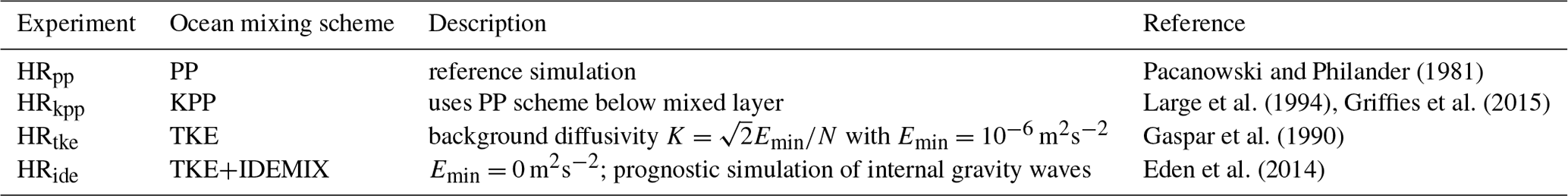
The reference simulation (HR_pp) uses the PP scheme and exactly the configuration used by Müller et al. (2018) and Gutjahr et al. (2019). In the second simulation, we used the KPP scheme and refer to it as HR_kpp. The configuration of this experiment is exactly as in Gutjahr et al. (2019). These two simulations were also compared with higher-resolution versions (atmosphere and ocean) by Gutjahr et al. (2019), as part of the High-Resolution Model Intercomparison Project (HighResMIP; Haarsma et al., 2016).

The third experiment (HR_tke) used the TKE scheme with a background diffusivity that depends on the buoyancy frequency and on a minimum value for TKE (see Appendix A3) but without any contribution from IDEMIX. In the last experiment (HR_ide), we used the TKE scheme together with IDEMIX (TKE+IDEMIX) and replaced the artificial background diffusivity with one diagnosed from TKE that is fuelled by the internal wave dissipation (see Sect. A3 for more details). If not explicitly mentioned, we used default values for the parameters of the mixing schemes, as listed in the respective original description (see also Appendix A), without analysing the effect of changed parameters.

The initial state was derived from a MPI-ESM1.2-HR simulation (with the PP scheme) that was nudged to the averaged temperature and salinity state of 1950 to 1954 of the Met Office Hadley Centre EN4 observational data set (version 4.2.0; Good et al., 2013), as described in Gutjahr et al. (2019). All simulations were forced by constant 1950s conditions according to the HighResMIP protocol (Haarsma et al., 2016). As recommended in this protocol, the model was not retuned to obtain isolated effects from changing the ocean vertical mixing scheme. If not stated otherwise, we analysed averages over the last 20 model years (model years 81 to 100). Although our focus is on the ocean, we briefly present results for the atmosphere as well.

3 Effects on the global ocean

In the following, we present how the choice of the ocean vertical mixing scheme affects the ocean mean state in control simulations with MPI-ESM1.2-HR. We first present results for the global ocean before discussing specific regional aspects in Sect. 4.

3.1 Spatial distribution of vertical diffusivity

Figure 1 shows the spatial distribution of the vertical diffusivity K for the model layer at 1020 m depth. Apart from boundary flows, deep convection regions, and the surface mixed layer, K is approximately homogeneous in the simulations with PP and KPP. Both simulations use a simple constant background diffusivity of $K=\mathrm{1.05}\times {\mathrm{10}}^{-\mathrm{5}}$ m² s⁻² to parameterize internal wave breaking. Because of the relationship $K=\sqrt{\mathrm{2}}{E}_{\min }/N$ for the background diffusivity in the TKE scheme (see Appendix A3), HR_tke simulates a small K in the tropical and subtropical ocean, where N is positive, and a large K in the high-latitude ocean, where N is negative. Even more heterogeneous is the distribution of K in HR_ide, which simulates stronger mixing above rough topography and mixing coefficients of about 2 orders of magnitude lower above the abyssal plains and in the Arctic Ocean. Hotspots of strong vertical mixing are simulated for all four cases particularly in the subpolar North Atlantic (SPNA), in the Nordic Seas, and in the Weddell and Ross seas of the Southern Ocean. Excessive deep convection in the Weddell Sea is a known issue in ocean models (e.g. Sallée et al., 2013; Kjellsson et al., 2015; Heuzé et al., 2015; Naughten et al., 2018) and not unique to MPI-ESM1.2-HR. The unrealistic convection is related to anomalously frequent open-ocean Weddell Sea polynyas (Gordon, 1978; Carsey, 1980; Gordon, 2014). HR_ide reduces the occurrence of this spurious deep convection, which we will discuss in Sect. 4.4.

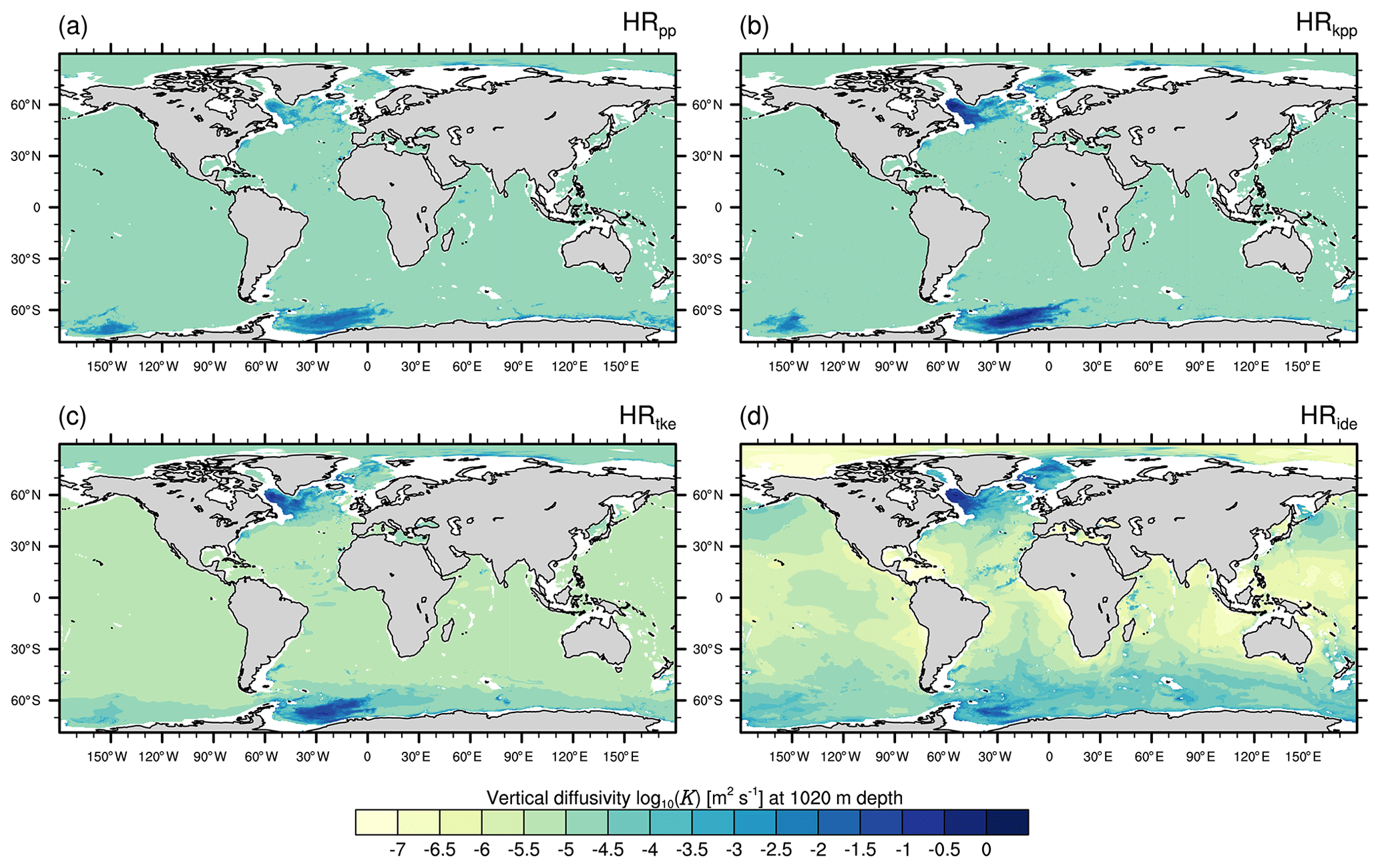
Figure 1 Time-averaged vertical diffusivity log ₁₀(K) (m² s⁻¹) at a depth of 1020 m in the MPI-ESM1.2-HR simulations for (a) HR_pp, (b) HR_kpp, (c) HR_tke, and (d) HR_ide.

A closer look at Fig. 1 reveals more regional differences in the above-mentioned areas. We will relate them to biases in temperature and salinity (Sect. 3.2 and 3.4) and discuss them in more detail for the SPNA and Nordic Seas (Sect. 4.1), the Fram Strait (Sect. 4.2), the Arctic Ocean (Sect. 4.3), and the Southern Ocean (Sect. 4.4).

3.2 Sea surface temperature and salinity bias

The sea surface temperature (SST) is a key quantity for the atmosphere–ocean coupling. Reducing biases of SST in model simulations is thus of crucial importance. However, the causes of SST biases are often complex and result, among others, from insufficient horizontal and vertical resolution and from the need to parameterize subgrid-scale processes, which has the largest influence on the biases (Fox-Kemper et al., 2019). Vertical mixing is thereby only one of these parameterizations.

Overall, the SSTs are mostly colder in the MPI-ESM1.2-HR simulations compared with EN4 (Fig. 2). Although vertical mixing has little effect on the SST bias in large parts of the ocean, some areas are more sensitive. One such area is the North Atlantic with its subpolar gyre, as well as the Nordic Seas. The largest cold bias occurs in the North Atlantic and amounts to −7 ^∘C in HR_pp. This cold bias is a common phenomena in ocean models (e.g. Randall et al., 2007) and is mainly caused by a too-zonal pathway of the Gulf Stream (Dengg et al., 1996) in relation to insufficient horizontal resolution and northward heat transport (Wang et al., 2014). By using a vertical mixing scheme other than PP, we find that the SST cold bias in the North Atlantic is reduced (Fig. 2b–d). This reduction of the cold bias can be explained by a generally warmer North Atlantic. A stronger Atlantic meridional overturning circulation (AMOC) in the simulations with KPP and TKE (see Sect. 3.5) transports more heat northwards that leads to warmer temperatures in the SPNA, especially in the Labrador and Irminger seas, and in the Nordic Seas.

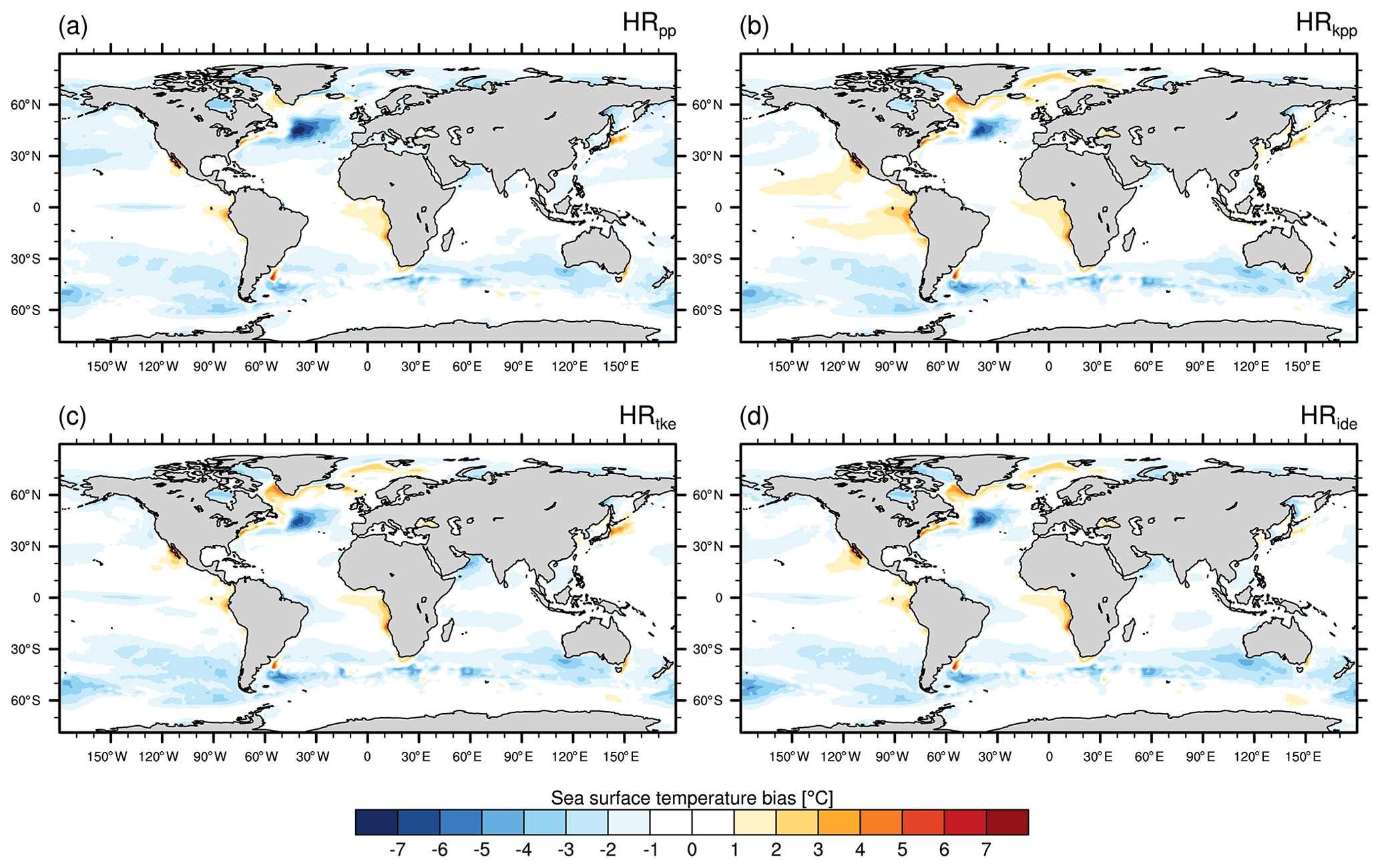
Figure 2 Time-averaged sea surface temperature bias of MPI-ESM1.2-HR minus EN4 (1945–1955) for (a) HR_pp, (b) HR_kpp, (c) HR_tke, and (d) HR_ide.

Strong warm biases occur also in the tropical upwelling regions off the west coasts of Africa and South America, which are related to insufficiently resolved coastal winds that force the upwelling of colder water (Milinski et al., 2016).

The sea surface salinity is mostly unaffected by the chosen vertical mixing scheme, except in the Arctic Ocean (Fig. 3) and in the western and eastern equatorial Pacific, which could be related to differences in the feedback with the atmosphere. By using the TKE or TKE+IDEMIX scheme, the salinity bias is considerably reduced, especially in the Canada Basin (Fig. 3c–d). The cause for these fresher surface waters is not yet well understood. Most likely it is linked to the reduced sea ice formation that we will discuss in the next section.

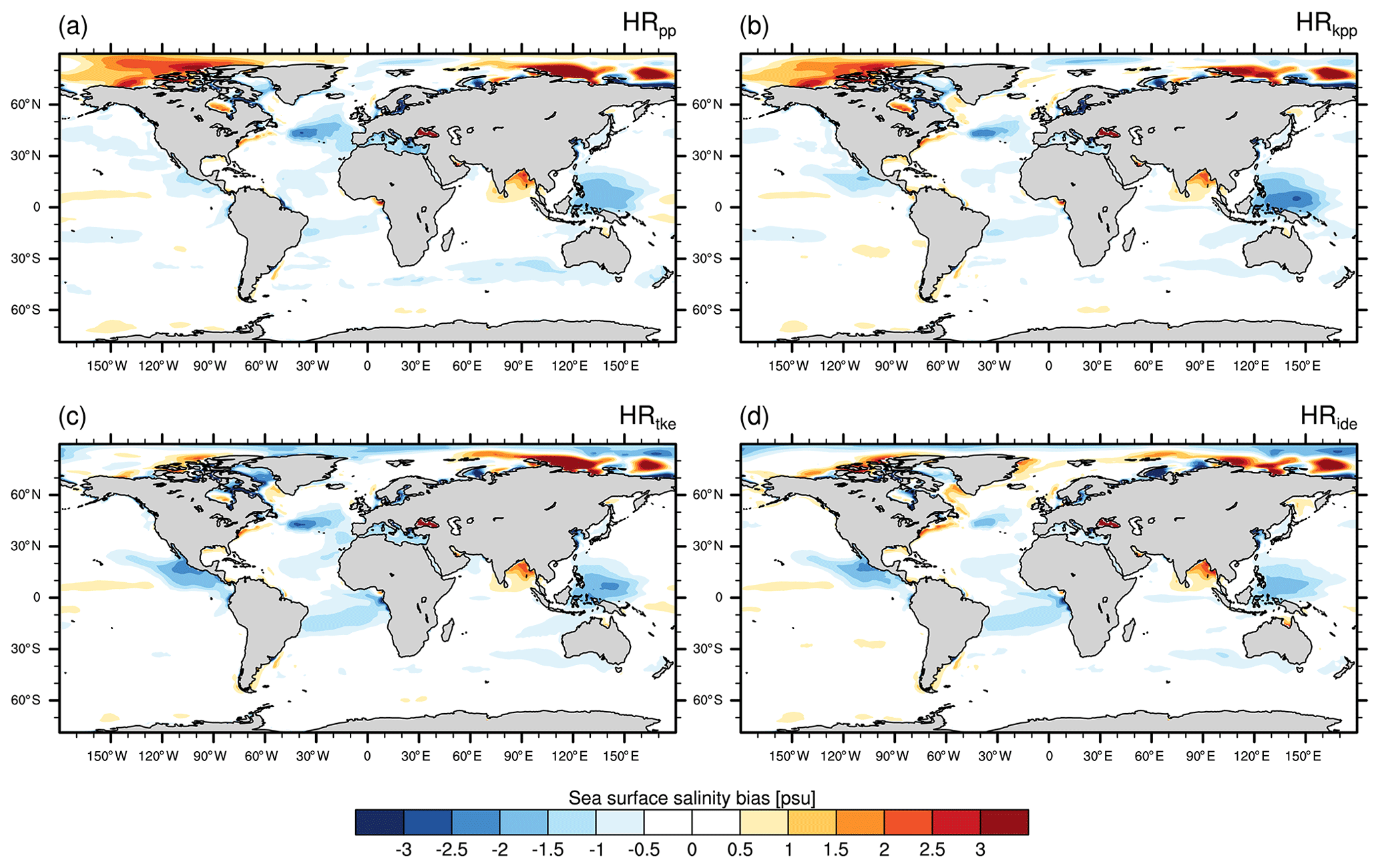
Figure 3 Time-averaged sea surface salinity bias of MPI-ESM1.2-HR minus EN4 (1945–1955) for (a) HR_pp, (b) HR_kpp, (c) HR_tke, and (d) HR_ide.

3.3 Sea ice

The extent and thickness of sea ice in March in the Arctic Ocean and the Nordic Seas are shown in Fig. 4. We compare the sea ice thickness to average thickness (1979–2005) of the Pan-Arctic Ice-Ocean Modeling and Assimilation System (PIOMAS) reanalysis (Zhang and Rothrock, 2003; Schweiger et al., 2011). We define the ice edge as the 15 % ice concentration and compare it with the European Organisation for the Exploitation of Meteorological Satellites (EUMETSAT) Ocean and Sea Ice Satellite Application Facility (OSI SAF) (OSI-409-a; v1.2) product (1979–2005) (EUMETSAT Ocean and Sea Ice Satellite Application, 2015).

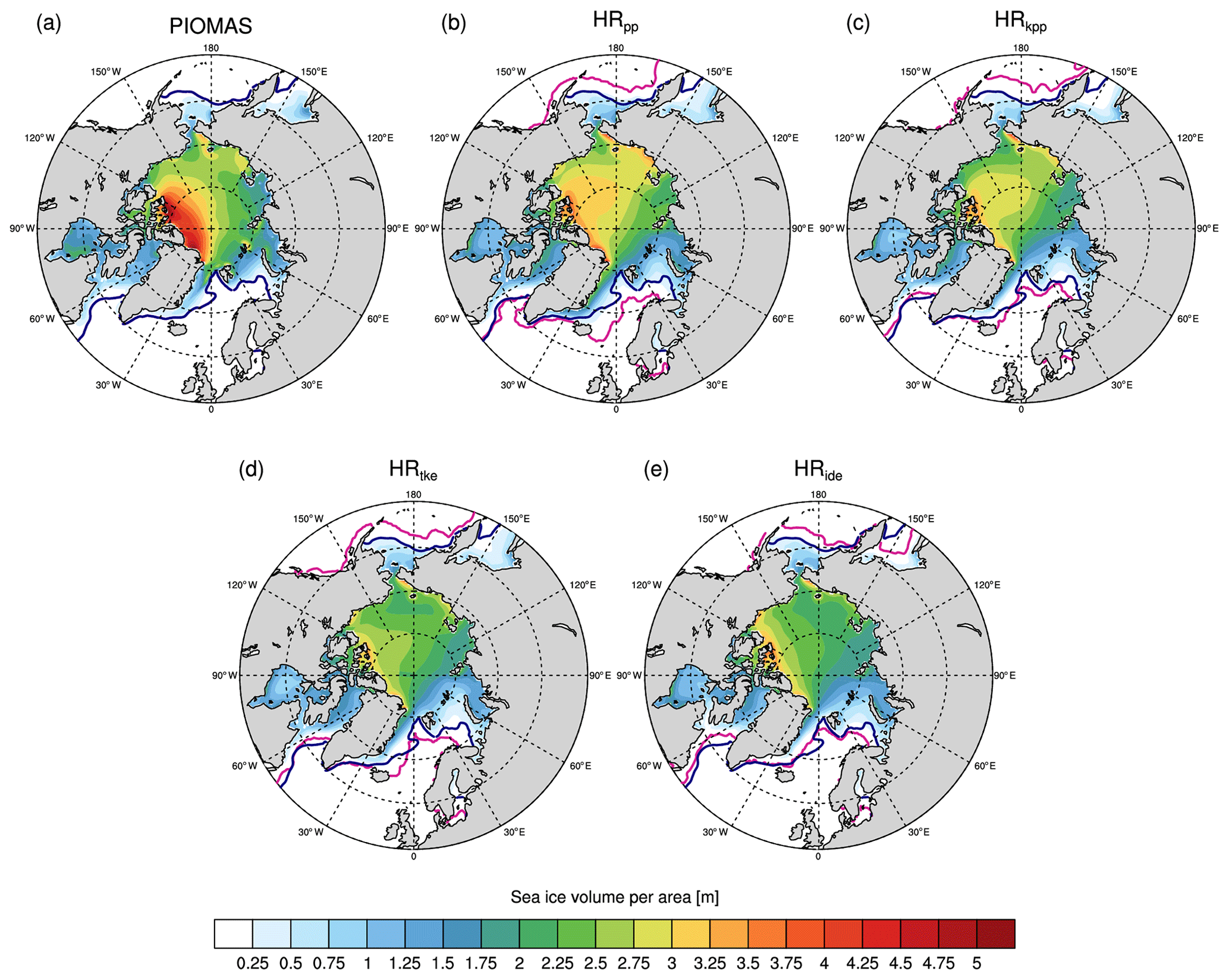
Figure 4 Time-averaged Arctic sea ice thickness in March for (a) PIOMAS reanalysis (March 1979–2005; Zhang and Rothrock, 2003; Schweiger et al., 2011), (b) HR_pp, (c) HR_kpp, (d) HR_tke, and (e) HR_ide. The 15 % sea ice concentration of the EUMETSAT OSI SAF (averaged over March 1979–2005) is contoured in dark blue and those of the simulations in magenta.

The ice extent is largest in the reference simulation with the PP scheme (Fig. 4a). The ice edge extends further south everywhere than in PIOMAS, especially in the Nordic Seas and the Labrador Sea. The ice edge in the Labrador Sea and the Nordic Seas lies further north in the simulations with KPP and TKE(+IDEMIX), especially in HR_ide. In the North Pacific, the ice edge is less affected and lies only further north in the Sea of Okhotsk in HR_ide. The more northerly location of the ice edge in the KPP and TKE(+IDEMIX) simulations than in HR_pp results from warmer water temperatures in the Nordic Seas and Labrador Sea, which causes the sea ice to retreat.

Ice thickness is lower in all simulations compared to PIOMAS, especially in the central Arctic and north of Greenland, and lowest in HR_ide. What causes thinner ice in the simulations with KPP and TKE(+IDEMIX) is unclear and remains for further investigation. It could be related to lower ice production in the marginal seas, especially in the Laptev Sea, and could require further tuning of the lead-close parameterization.

In the Southern Hemisphere, there is also thinner ice simulated with the TKE and TKE+IDEMIX scheme for the time-averaged September (Fig. 5), especially along the coast of Antarctica. However, we note a closed sea ice cover in the Weddell Sea in HR_ide that reduces spurious convection within the Weddell Sea polynya (see more details in Sect. 4.4.1). The sea ice extent is larger than in OSI SAF but differs only slightly between the simulations.

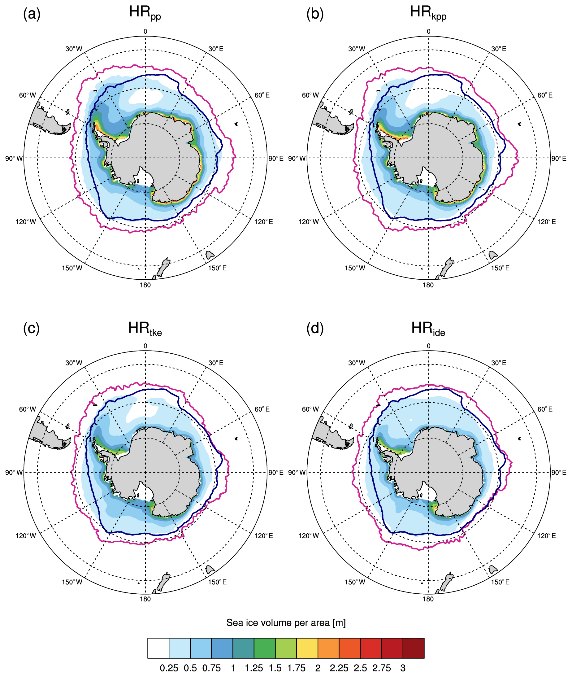
Figure 5 Time-averaged Arctic sea ice thickness in March for (a) HR_pp, (b) HR_kpp, (c) HR_tke, and (d) HR_ide. The 15 % sea ice concentration of the EUMETSAT OSI SAF (averaged over March 1979–2005) is contoured in dark blue and those of the simulations in magenta.

3.4 Ocean interior

3.4.1 Horizontal maps of hydrographic biases

At intermediate depth, all simulations are too warm compared to EN4, as shown by the temperature bias for the model layer at 740 m depth (Fig. 6). Exceptions are the Southern Ocean and parts of the North Atlantic, where the ocean is colder at upper to intermediate depth. In the Atlantic Ocean, the warm biases are mainly linked to the representation of the Agulhas Current system and Mediterranean Overflow Water (MOW), as well as to the pathway of the Gulf Stream. Previous studies with MPI-ESM1.2 have shown that these warm biases diminish with increasing spatial resolution (Gutjahr et al., 2019; Putrasahan et al., 2019). Advection of these warmer (and more saline) water masses causes subsequent warm biases in the SPNA, Nordic Seas, and Arctic Ocean. Even though an eddy-resolving resolution (0.1^∘) reduces most of these biases, as shown by Gutjahr et al. (2019) with MPI-ESM1.2-ER, the choice of the vertical mixing scheme also affects the hydrographic biases; for instance, with TKE+IDEMIX, the warm bias is reduced in the Arctic Ocean but enhanced for the MOW (Fig. 6).

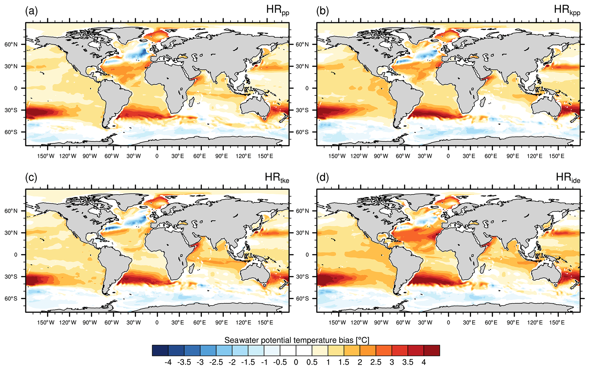
Figure 6 Time-averaged potential temperature bias of MPI-ESM1.2-HR minus EN4 (1945–1955) at a depth of 740 m for (a) HR_pp, (b) HR_kpp, (c) HR_tke, and (d) HR_ide.

Salinity shows a similar bias pattern at intermediate depth (Fig. 7). The Atlantic is too saline, which is again due to the poor representation of the MOW and the Agulhas Current system. Consequently, northward advection by the Gulf Stream and the boundary currents along the European shelf distribute these saline waters into the SPNA and Nordic Seas, where they affect the local water masses (Reid, 1979; McCartney and Mauritzen, 2001; Lozier and Sindlinger, 2008). At a resolution of 0.4^∘, MPI-ESM1.2-HR is unable to capture the Agulhas Retroflection. Although all simulations show a similar salinity bias in the Agulhas region, we note a larger bias for HR_kpp, HR_tke, and HR_ide. This larger bias indicates a stronger inflow of warm and salty water from the Indian Ocean. In fact, the inflow is about 10 Sv stronger with TKE(+IDEMIX) and about 15 Sv with KPP than the 40 to 50 Sv in HR_pp (Fig. 8). We further notice a large salinity bias in all simulations in the South Pacific that seems to be linked to the South Pacific gyre. We speculate that the bias is due to unresolved eddies in the East Australian Current and processes at the border zone of the South Pacific Current and the Subantarctic Front. A more detailed analysis is needed to identify the cause of this model bias, which we suspect to be related to model resolution but will not explore here.

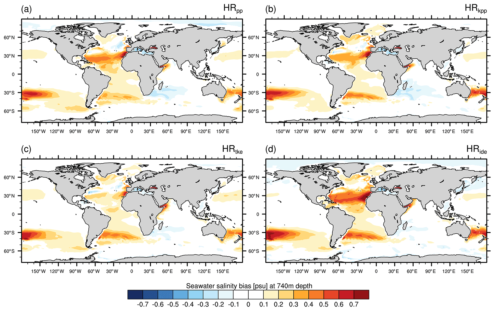
Figure 7 Time-averaged salinity bias of MPI-ESM1.2-HR minus EN4 (1945–1955) at a depth of 740 m for (a) HR_pp, (b) HR_kpp, (c) HR_tke, and (d) HR_ide.

The largest difference in salinity bias is linked to the representation of MOW. Although all models produce warmer and more saline MOW, the bias is decreased only in HR_tke. The bias even becomes considerably larger when TKE is used with IDEMIX instead of an artificial background diffusivity (Fig. 7d). Although the use of IDEMIX increases vertical eddy diffusivity at the overflow sill of the Strait of Gibraltar and in the Gulf of Cádiz (not shown), downstream vertical mixing over the abyssal plains of the Atlantic is very low, probably due to the low internal wave activity, so that the diffusivity becomes very low (O(10⁻⁶ m² s⁻²)). We speculate that this lower diffusivity reduces mixing with the overlying, less saline North Atlantic Central Water, so that the warm, highly saline core of the MOW is less diluted than in the other simulations. However, the MOW is already saltier by about 0.4 psu and 0.5 ^∘C warmer before it flows into the Atlantic. It remains a subject of further investigation what causes this warmer and saltier MOW in TKE+IDEMIX. Possibly, the scheme modifies the variability of the near-surface wind field or the net evaporation over the Mediterranean Sea (Aldama-Campino and Döös, 2020).

We further note a slight freshwater bias in the Arctic Ocean in HR_ide that we will describe in relation to the Atlantic Water layer in Sect. 4.2.

3.4.2 Vertical sections through the Atlantic and Arctic oceans

A vertical section of the zonally averaged potential temperature bias through the Atlantic and Arctic Oceans (Fig. 9) shows predominantly too-cold near-surface water, especially in the North Atlantic, where the cold bias extends to a depth of about 1000 m due to errors in heat convergence resulting from a misrepresented Gulf Stream and North Atlantic Current. The intermediate water masses are too warm compared with EN4 and there appears almost no bias in the deeper ocean, since the simulation length is too short to affect the abyssal ocean. This general bias pattern is established in all simulations, but we note some differences.

Figure 8 Time-averaged, vertically integrated volume transport in the Agulhas region south of Africa as simulated by MPI-ESM1.2 (a) HR_pp and the difference (experiment minus HR_pp) for (b) HR_kpp, (c) HR_tke, and (d) HR_ide.

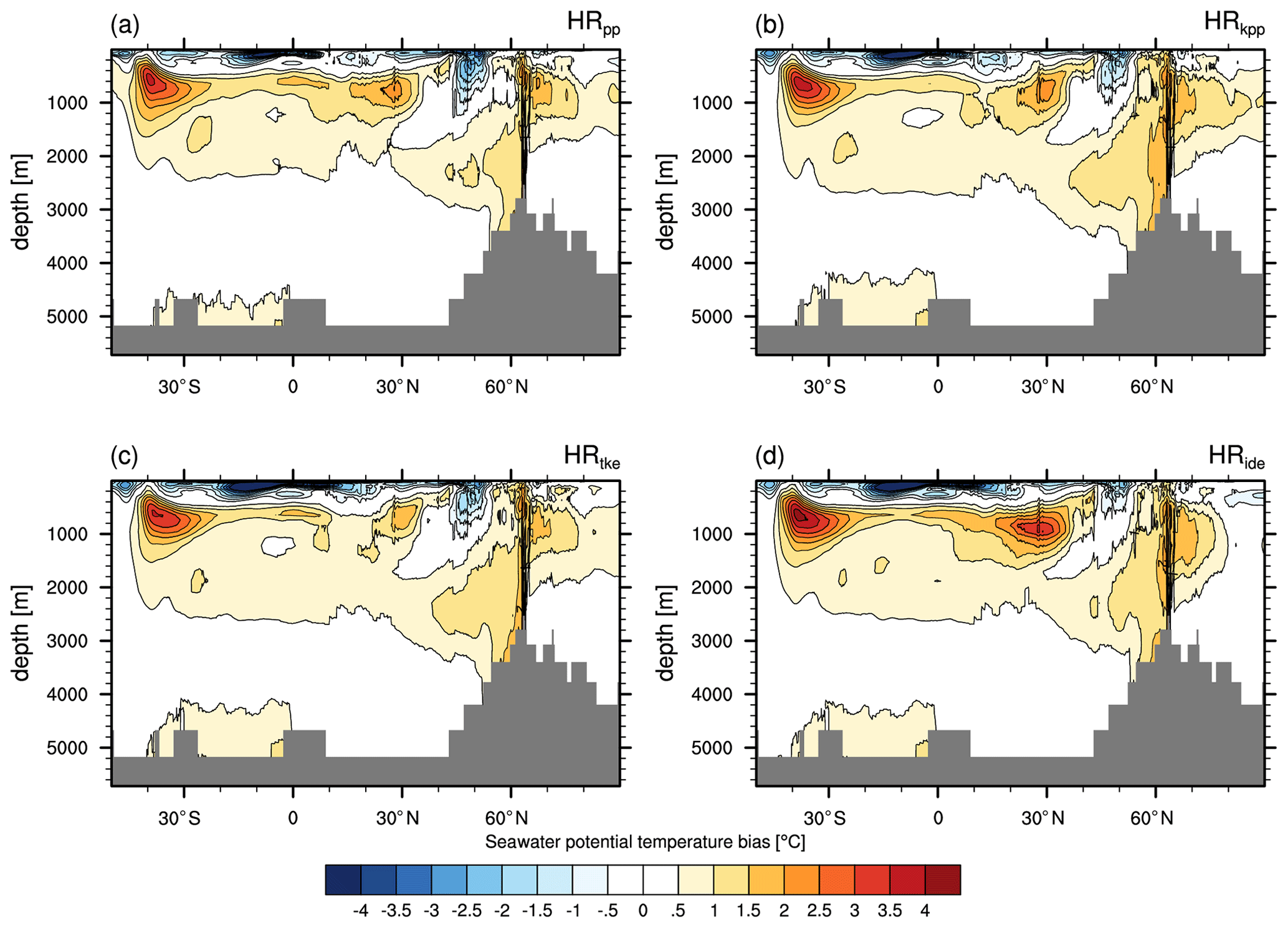
Figure 9 Zonal-mean potential temperature bias of MPI-ESM1.2-HR minus EN4 (1945–1955) in the Atlantic and Arctic Ocean for (a) HR_pp, (b) HR_kpp, (c) HR_tke, and (d) HR_ide.

All simulations simulate a too-warm (and saline) inflow from the Indian Ocean to the South Atlantic, roughly at 30^∘ S. The model resolution is too coarse to correctly capture the Agulhas Current system; in particular, the retroflection and Agulhas rings are not well represented. Instead, warm and saline water flows more or less constantly from the Indian Ocean into the South Atlantic. From all simulations, this misrepresentation is strongest in HR_ide. The reason for this behaviour remains a subject for future studies.

A second source of too-warm water is related to the MOW, as described above. The core of the MOW reaches a neutral buoyancy surface slightly above 1000 m depth at roughly 30^∘ N. The MOW is warmest in HR_ide but colder in HR_tke compared to the reference simulation.

These already-too-warm waters are transported north throughout the whole Atlantic and eventually reach the SPNA and Nordic Seas. Part of it continuous further into the Arctic Ocean at a depth of 500 m to more than 1000 m, where it becomes the Atlantic Water (AW) layer, which is roughly 1 ^∘C warmer than in EN4. Due to stronger recirculation in Fram Strait (see Sect. 4.2), less AW enters the Arctic Ocean in HR_ide, reducing the warm bias.

In the Nordic Seas, the water temperature is higher in all simulations with KPP and TKE(+IDEMIX) than in HR_pp. Although the higher temperature partly compensates for the increase in salinity, the overflows across the Greenland–Iceland–Scotland Ridge are dense enough and reach depths of about 3000 m. Their warmer temperature can be seen at and south of 60^∘ N. Similarly, also the deep water formed in the Labrador Sea is warmer than in HR_pp and together these water masses cause a warm bias when exported as the Deep Western Boundary Current.

Salinity shows a similar bias pattern (not shown) with too-saline waters where there is a warm bias.

3.5 AMOC and transport

The SPNA and the Nordic Seas are important regions for the global climate, where the vertical connection between the upper warm and the lower cold branch of the AMOC is established. The northward-flowing warm AW is cooled by extensive heat loss to the atmosphere until it becomes dense enough to sink into deeper layers. Together with the dense overflow water from the Nordic Seas, it leaves the SPNA as North Atlantic Deep Water (NADW) with the southward-flowing Deep Western Boundary Current (DWBC).

The simulations with KPP and TKE(+IDEMIX) produce a stronger and deeper-reaching upper branch of the AMOC of >18 Sv at 26.5^∘ N (Fig. 10) compared with about 15 Sv in HR_pp. A stronger upper cell may imply a stronger northward heat transport, whereas a deeper upper cell indicates a stronger southward transport of NADW (see Sect. 4.1.2). To compensate for the increased overturning in the Nordic Seas, the water in the Atlantic must be replaced by a stronger inflow from the Indian Ocean, which is the case in the simulations with KPP and TKE(+IDEMIX), as seen in Fig. 8.

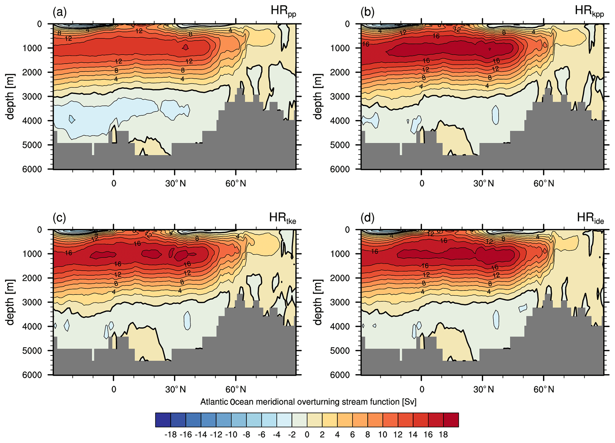
Figure 10 Eulerian stream function (Sv =10⁶ m³ s⁻¹) of the AMOC in depth space simulated by MPI-ESM1.2 (a) HR_pp, (b) HR_kpp, (c) HR_tke, and (d) HR_ide.

Figure 11 Time-averaged vertical diffusivity log ₁₀(K) (m² s⁻¹) at a depth of 690 m in the subpolar North Atlantic simulated by MPI-ESM1.2 (a) HR_pp, (b) HR_kpp, (c) HR_tke, and (d) HR_ide.

We note, however, that the bottom cell is weaker in all sensitivity simulations, which is probably due to a stronger mixing of NADW with Antarctic Bottom Water (AABW), causing the latter to vanish further south. The simulation length of 100 years is too short to see pronounced effects in the deep ocean, but it could be expected that over longer periods (several centuries) the additional mixing from internal waves might affect the diapycnal diffusion of the upwelling deep water, e.g. in the Pacific.

4 Effects on the regional ocean

In this section, we discuss some regional areas in more detail, in particular the Atlantic Ocean, the Nordic Seas and Fram Strait, the Arctic Ocean, and the Southern Ocean. We already note here that the insufficient model resolution determines the large-scale bias pattern, as shown by Gutjahr et al. (2019).

4.1 Subpolar North Atlantic and the Nordic Seas

4.1.1 Convection and mixed layer depths

The sinking of buoyant Atlantic Water is thought to be established by downwelling of dense water along the boundary currents with complex interplay of deep convection and the mesoscale eddy field (e.g. Katsman et al., 2018; Brüggemann and Katsman, 2019; Sayol et al., 2019; Georgiou et al., 2019). The water mass transformation of Atlantic Water occurs, however, in areas of deep convection and lateral exchange with the boundary current by eddies. Convection, or vertical instability, is parameterized differently in the vertical mixing schemes in MPI-ESM1.2 (see Appendix A), which is why we expect differences in vertical diffusion and mixed layer depths (MLDs). Eddies are only partially resolved in MPI-ESM1.2-HR, so we do not expect the exchange of deep water with the boundary currents to be realistic.

The largest diffusivities (K) are simulated in the Labrador Sea and the Nordic Seas (Fig. 11), with markedly greater values in the simulations with KPP and TKE(+IDEMIX). In particular, we note increased vertical diffusivities in the Irminger Sea, where open-ocean deep convection occurs and contributes to the formation of Labrador Sea water (e.g. Pickart et al., 2003; Våge et al., 2011).

In the PP scheme, the vertical instability is parameterized by enhancing the diffusivity to K=0.1 m² s⁻¹. The convection parameterization in KPP is more complex, where non-local transport terms (see Appendix A2) redistribute the surface fluxes throughout the ocean surface boundary layer. These non-local transport terms depend on the net heat and freshwater fluxes at the ocean surface, on K, and on a dimensionless vertical shape function (Large et al., 1994; Griffies et al., 2015).

In the TKE scheme, the buoyancy term (third term on the right-hand side of Eq. A15), which usually is an energy transfer from TKE to mean potential energy, acts in this case (N²<0) in the opposite direction and enhances TKE. However, besides differences in the parameterizations, remotely changed water mass properties, and hence density changes, also affect convection and the MLD in the SPNA. Therefore, it is not straightforward to diagnose what is a cause and what is a consequence for changes in the MLDs.

The average MLDs in March are shown in Fig. 12. A direct comparison with MLDs derived from Argo floats is not optimal, because our simulations are control simulations with 1950s greenhouse gas forcing. Keeping this in mind, we find profound differences to Argo-float-derived MLDs and across the simulations. As with vertical diffusivity, all simulations show the deepest mixed layers in the Labrador Sea and a second maximum in the Greenland–Iceland–Norway (GIN) seas. In general, KPP and TKE(+IDEMIX) tend to simulate deeper mixed layers. In the Labrador Sea, the convection area extends too far north in all simulations due to the lack of mesoscale eddies that would impede convection by restratification of the water column (e.g. Eden and Böning, 2002; Brüggemann and Katsman, 2019; Gutjahr et al., 2019). HR_ide simulates deeper mixed layers in the centre of the Greenland Sea gyre and particular around Jan Mayen, which might be caused by internal wave activity, especially along the Kolbeinsey and Mohn ridges and along the Jan Mayen Fracture Zone.

Figure 12 Time-averaged mixed layer depths (m) in March calculated by the density threshold method (σ_t=0.03 kg m⁻³) from (a) $\mathrm{1}{}^{\circ }\times \mathrm{1}{}^{\circ }$ Argo float data (Holte et al., 2017) (mean March from 2000 to 2018) and from MPI-ESM1.2 (b) HR_pp, (c) HR_kpp, (d) HR_tke, and (e) HR_ide.

Due to stronger updoming of the isopycnals in the Labrador, Irminger, and Greenland seas in the simulations with KPP and TKE(+IDEMIX), the strength of the gyres is stronger than in HR_pp (Fig. 13). This enhanced updoming is caused by a combination of a more saline SPNA and Nordic Seas, e.g. about +0.2 psu in the Greenland Sea, and enhanced heat loss in the gyre centres. The steeper isopycnal gradients accelerate the geostrophic flow around the convection centres leading to a roughly 10 Sv stronger boundary current in the Labrador Sea and a Greenland gyre that is about 5 Sv stronger.

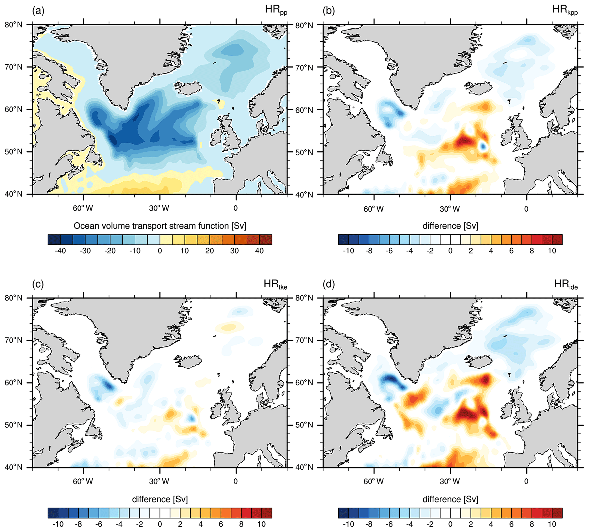
Figure 13 Time-averaged barotropic volume transport stream function (Sv) in the North Atlantic as simulated by MPI-ESM1.2 (a) HR_pp, and the differences of “experiment – HR_pp” for (b) HR_kpp, (c) HR_tke, and (d) HR_ide.

4.1.2 Overflows from the Nordic Seas

A substantial contribution to the NADW constitutes the Denmark Strait overflow water (DSOW; σ>1027.8 kg m⁻³), which accounts for about half of the observed overflows from the Nordic Seas (Hansen et al., 2004), being its densest water mass. The other major overflow pathway across the Greenland–Iceland–Scotland Ridge is through the Faroe–Shetland Channel (FSC; σ>1027.75 kg m⁻³) and through the Faroe Bank Channel (FBC; σ>1027.75 kg m⁻³).

The increased MLDs in the simulations with KPP and TKE(+IDEMIX) due to stronger deep convection in the Nordic Seas suggest higher overflow volumes. We applied Welch's two-sided t tests with α=0.05 (n=20) to test for significant differences in the simulated overflows. See Table A1 for all test results.

First, we note that all simulations underestimate the observed DSOW volume transport of about 3.2 to 3.4 Sv by roughly 1 Sv (see Table 2). Compared with HR_pp, however, we find about 10 % to 20 % higher DSOW transport in HR_kpp, HR_ide and especially in HR_tke (all with p<0.01). The transport in the KPP and TKE simulations, however, does not differ significantly (p values of 0.13 to 0.52). The higher amount of DSOW might thus explain at least partly the stronger upper cell of the AMOC and in particular the AMOC strength around 60^∘ N.

Jochumsen et al. (2017)Jochumsen et al. (2012)Hansen et al. (2016)Berx et al. (2013)Hansen et al. (2015)Rossby and Flagg (2012)Childers et al. (2014)

Table 2 Time-averaged volume transport (1 Sv=10⁶ m³ s⁻¹) of Denmark Strait overflow water (DSOW), Faroe Bank Channel (FBC), and Faroe–Shetland Channel (FSC) overflow from simulations with MPI-ESM1.2-HR. Hansen et al. (2017) note that measurements by Rossby and Flagg (2012) and Childers et al. (2014) include a closed circulation on the Faroe Shelf (0.6 Sv) and flow on the Scottish Shelf, which are not included in measurements by Berx et al. (2013) and Hansen et al. (2015). A standard deviation based on annual averages is given for the simulations.

Although they are overestimated compared to the observations, the FSC overflows in the simulations are of similar magnitude (3.2 to 3.3 Sv), with the exception of HR_tke, which produces an approximately 10 % higher (3.5 Sv) overflow transport (p<0.01). The FBC overflows are about 15 % to 20 % lower in the models (1.7 to 1.9 Sv) than the observed 2.2 Sv by Hansen et al. (2016). The deviations between the models are of the order of 10 %, with a higher mean transport in HR_tke (p<0.01) and a lower transport in HR_ide (p<0.01).

Overall, these results suggest about 10 % higher overflow is transported across the Greenland–Iceland–Scotland Ridge with KPP and TKE, which contributes to a stronger upper cell of the AMOC.

4.2 Fram Strait and Atlantic Water layer

AW is the main supplier of salt and oceanic heat to the Arctic Ocean. From the Nordic Seas, it flows northwards into Fram Strait, where about half of the AW recirculates southwards between 76 and 81^∘ N and becomes part of the East Greenland Current. A smaller fraction continues northward as the West Spitsbergen Current (WSC). Due to the successive cooling in its path, the subsiding AW flows into the Arctic Ocean at mid-depth with its core at about 400 m depth, sealed off from the atmosphere by overlying cold polar surface water.

A common error of many state-of-the-art ocean models is an anomalously thick and deep AW layer (e.g. Holloway et al., 2007; Shu et al., 2019). This error is thought to be related to model resolution and to vertical mixing parameterizations, in particular to the choice of the background diffusivity (Zhang and Steele, 2007; Liang and Losch, 2018). In terms of model resolution, it was recently shown that a high-resolution ocean (0.1^∘ or better) reduces biases of the AW layer (Wang et al., 2018; Gutjahr et al., 2019), because eddies are (partly) resolved that also improve the circulation (Wekerle et al., 2017). MPI-ESM-HR at eddy-permitting resolution produces a too-warm AW layer, as shown by Gutjahr et al. (2019). Here, we demonstrate that this warm bias is reduced by using TKE+IDEMIX, which is due to a combination of remote (already colder inflowing AW into the Fram Strait) and local effects (stronger southward recirculation in the Fram Strait and stronger heat loss due to enhanced mixing).

In HR_pp, HR_kpp, and HR_tke, the warm bias of the AW layer is about +2 ^∘C at the Yermak Plateau (YP), a bathymetric feature northwest of the Svalbard archipelago known as a hotspot for internal wave activity (see also Fig. A2b) and mixing (e.g. Fer et al., 2010; Crews et al., 2019), and less further downstream along the shelf break of the Eurasian Basin (Fig. 14). It seems that a part of the AW also crosses the Lomonosov Ridge, except in HR_ide, and spreads into the Markarov and Canada basins, which is not realistic. The AW is colder in HR_ide and better agrees with EN4 in the Eurasian basin, although the central Arctic Ocean becomes about 0.5 ^∘C too cold.

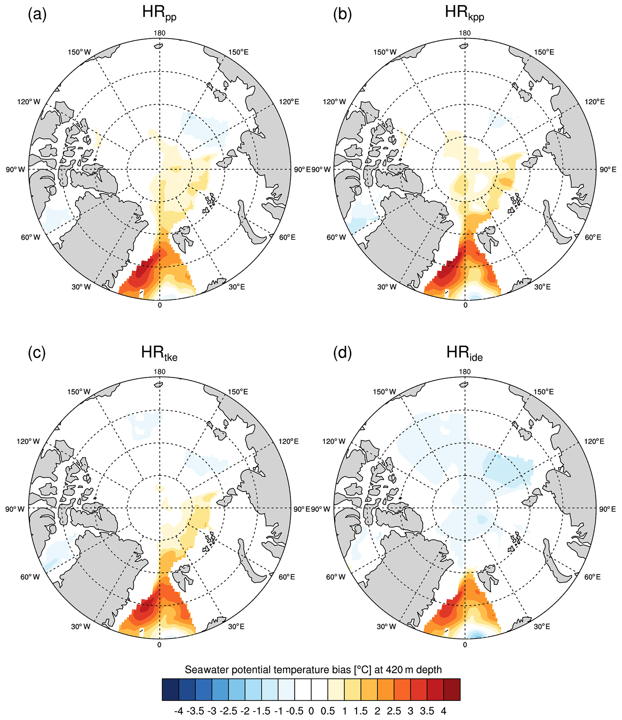
Figure 14 Time-averaged potential temperature bias of MPI-ESM1.2-HR minus EN4 (1945–1955) at a depth of 420 m in the Arctic Ocean and the Fram Strait for (a) HR_pp, (b) HR_kpp, (c) HR_tke, and (d) HR_ide.

Due to stronger heat loss in the Greenland Sea (not shown), the Atlantic Water is already about 1 ^∘C colder in HR_ide compared with the other simulations when it reaches Fram Strait, although warmer AW could be expected due to the stronger Greenland Sea gyre (Chatterjee et al., 2018; Muilwijk et al., 2019). This contradiction can be explained by a stronger recirculation of AW in HR_ide in Fram Strait, which means that less AW flows in the Arctic Ocean and thus there is less heat.

Beside this remote effect, there are local effects related to enhanced mixing at the YP. A comparison of K of the model layer at 450 m depth (Fig. 15) shows that the mixing near the YP in HR_ide is slightly stronger (Fig. 15d). Internal waves break near the YP and thus transfer energy to small-scale turbulence. This effect is larger in the prognostic IDEMIX than from the assumed constant background diffusivity. The increased mixing in the ocean causes more heat loss, as more warm AW is exposed to the cold atmosphere and thus cools more efficiently than in the other simulations. In fact, the sensible heat flux is about 20 to 40 W m⁻² larger in HR_ide than in HR_pp (not shown). For comparison, the sensible heat flux is only about 10 to 20 W m⁻² stronger in HR_kpp and HR_tke.

Figure 15 Time-averaged vertical diffusivity log ₁₀(K) (m² s⁻¹) at a depth of 450 m in the Arctic Ocean and the Fram Strait simulated by MPI-ESM1.2 (a) HR_pp, (b) HR_kpp, (c) HR_tke, and (d) HR_ide. YP: Yermak Plateau, STA: St. Anna Trough, LR: Lomonosov Ridge. The yellow point marks the approximate position (89^∘ N, 7^∘ W) of the Barneo ice camp in the Amundsen Basin, where K on the $O\left({\mathrm{10}}^{-\mathrm{6}}{\mathrm{m}}^{\mathrm{2}}{\mathrm{s}}^{-\mathrm{1}}\right)$ was measured below the mixed layer (Fer, 2009).

4.3 Arctic Ocean

Although largely unknown, sparse observations indicate that turbulence in the Arctic Ocean is typically weak (Rainville and Winsor, 2008; Fer, 2009). The wind stress cannot act on the sea surface because of the insulating sea ice cover, which is why the effect of the wind stress on vertical mixing decreases quadratically with the sea ice concentration in the simulations with PP and KPP (see Appendix A). In addition, brine rejection in the interior Arctic is less effective as a mixing mechanism because of the strong stabilizing vertical salinity gradient. Therefore, apart from enhanced mixing by episodic shear events, storms during ice-free conditions (Rainville and Woodgate, 2009), mesoscale eddies, or lateral intrusion along the boundaries, vertical diffusive mixing dominates over turbulent mixing (Fer, 2009).

Internal wave activity is almost absent, except above rough topographic features. In fact, internal waves are trapped at the place of their origin and do not propagate far into the Arctic Ocean. This trapping occurs because the Arctic Ocean is north of the critical latitude, which is 74.5^∘ N for the M₂ tide, beyond which the Earth's rotation prohibits freely propagating internal waves. As a result, they dissipate at or very close to their source region with properties similar to lee waves (Rippeth et al., 2015, 2017).

For this reason, there is little or no contribution to small-scale turbulence in the inner Arctic Ocean in HR_ide, especially in the deep and flat-bottomed Canada Basin. The eddy diffusivity K is up to 2 orders of magnitude smaller (O(10⁻⁶ to 10⁻⁷ m² s⁻¹)) in HR_ide compared to the other simulations (Fig. 15), in which K is mostly at the constant background value ($\mathrm{1.05}\times {\mathrm{10}}^{-\mathrm{5}}$ m² s⁻¹).

Representing this trapping of internal waves is crucial to simulate eddy diffusivities that are more consistent with microstructure measurements, which show low eddy diffusivities in deep, flat-bottomed basins but elevated diffusivities above deep topography (Rainville and Winsor, 2008). The low diffusivities in deep basins agree well with observations from the Barneo ice camp drift, where $O\left({\mathrm{10}}^{-\mathrm{6}}{\mathrm{m}}^{\mathrm{2}}{\mathrm{s}}^{-\mathrm{1}}\right)$ was measured below the mixed layer in the Amundsen Basin (Fer, 2009).

Lower vertical diffusivity under sea ice in the Arctic Ocean might cause denser water to enter the Nordic Seas (Kim et al., 2015), which could then lead to denser overflows across the Greenland–Iceland–Scotland Ridge and a 14 % stronger upper cell of the AMOC. Indeed, HR_ide generates higher overflow volumes and a 10 % stronger AMOC, but these are probably caused more by denser water masses in the Greenland Sea. However, we cannot rule out the effect of denser water from the Arctic Ocean.

A contrasting example of higher diffusivities in the inner Arctic Ocean is a distinct band of strong mixing along and above the Lomonosov Ridge (Fig. 15d). Here, internal waves break immediately after their formation and thus locally increase the small-scale turbulence, a process that was also directly measured by Rainville and Winsor (2008).

Assuming a constant background diffusivity thus largely overestimates the vertical mixing in the Arctic Ocean. Although the background diffusivity can be artificially reduced to mimic this low internal wave activity (e.g. Kim et al., 2015; Sein et al., 2018), the very heterogeneous pattern described above would not be captured. The combination of TKE with IDEMIX is able to reproduce the spatial pattern and the correct magnitudes. It further provides an energetically more consistent solution that should be preferred.

4.4 Southern Ocean and Weddell Sea

4.4.1 Open-ocean convection in the Weddell Sea polynya

A well-known problem in ocean modelling is a too-frequent semi-permanent Weddell Sea polynya caused by false deep convection bringing warm Circumpolar Deep Water (CDW) close to the surface (Sallée et al., 2013; Kjellsson et al., 2015; Heuzé et al., 2015; Stössel et al., 2015; Naughten et al., 2018). Possible explanations are insufficient freshwater supply (Kjellsson et al., 2015), mainly due to a lack of glacier meltwater (Stössel et al., 2015), and insufficient wind mixing in summer (Timmermann and Beckmann, 2004; Sallée et al., 2013; Kjellsson et al., 2015), which causes a high salinity bias in the mixed layer that erodes the stratification; see a more detailed discussion in Gutjahr et al. (2019). In contrast to this view, Dufour et al. (2017) argue that deep convection in the Weddell Sea does not necessarily lead to an open-ocean polynya, because strong vertical mixing in low-resolution models inhibits the buildup of a subsurface heat reservoir that would be necessary for intermittent Weddell Sea polynyas.

We do not expect a realistic representation of the Weddell Sea polynya in our MPI-ESM1.2-HR 1950s control simulations, because they should develop intermittently only under pre-industrial conditions and grow out from Maud Rise polynyas (de Lavergne et al., 2014; Gordon, 2014; Kurtakoti et al., 2018; Campbell et al., 2019; Cheon and Gordon, 2019; Jena et al., 2019), for which high resolution (0.1^∘ or better) is required (Stössel et al., 2015; Dufour et al., 2017).

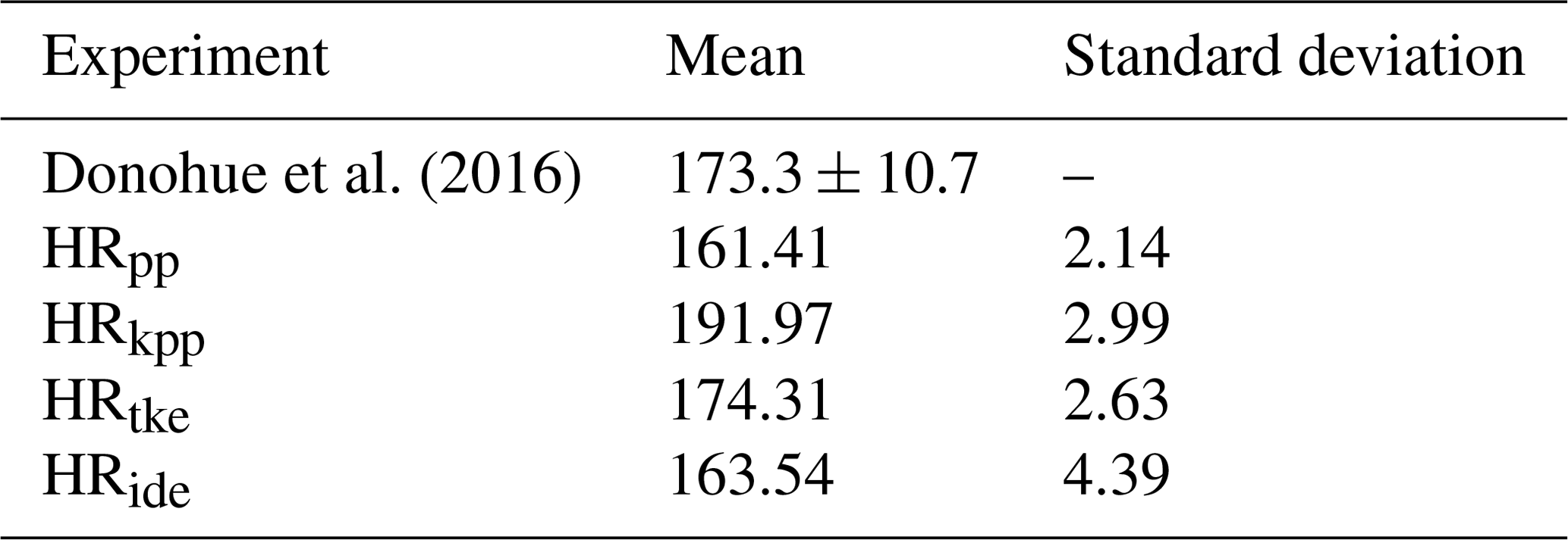
Although all simulations produce these semi-permanent Weddell Sea polynyas and thus too-deep mixed layers (Fig. 16), the area of excessive deep convection is reduced in HR_ide (Fig. 16e). Similarly, too-deep mixed layers are simulated in the Ross Sea, except in HR_tke, which simulates shallower mixed layers without further reduction when using IDEMIX (HR_ide). The Weddell Gyre is also linked to the Antarctic Circumpolar Current (ACC; Orsi et al., 1993; Cheon et al., 2019), because it controls the inflow of relatively warm and saline CDW into the inner Weddell Sea, possibly eroding the weak stratification and triggering deep convection. The simulated ACC transport through the Drake Passage (Table 3) is close to the recently observed 173.31±10.7 Sv (Donohue et al., 2016), whereby HR_tke achieves the best estimate with 174 Sv. Simulations with lower convection in the Weddell Sea produce lower transport of about 161 to 163 Sv (HR_pp and HR_ide), whereas HR_kpp produces a much higher transport of 192 Sv because of steeper isopycnals due to enhanced convection in the Weddell Sea. Since eddies are not resolved and the GM coefficient is rather low, there is no or too little eddy compensation to flatten the isopycnals.

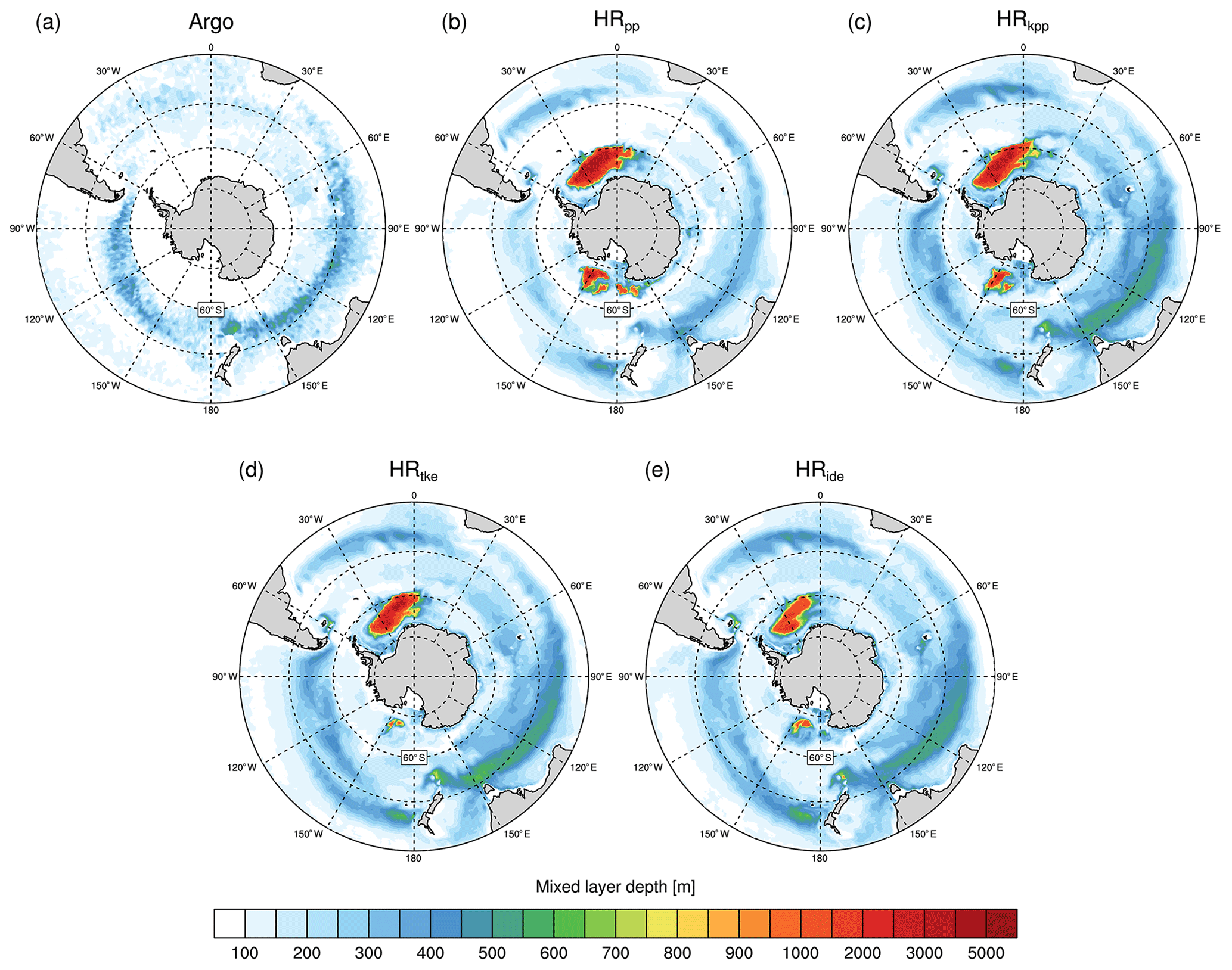
Figure 16 Time-averaged mixed layer depths (m) in September calculated (a) from $\mathrm{1}{}^{\circ }\times \mathrm{1}{}^{\circ }$ Argo float data (Holte et al., 2017) (mean September data from 2000 to 2018) by the density threshold method (σ_t=0.03 kg m⁻³) and from MPI-ESM1.2 (b) HR_pp, (c) HR_kpp, (d) HR_tke, and (e) HR_ide. Note that there are no Argo data south of 60^∘ S.

Donohue et al. (2016)

Table 3 Time-averaged volume transport (1 Sv=10⁶ m³ s⁻¹) of the Antarctic Circumpolar Current (ACC) through Drake Passage from observations and simulations with MPI-ESM1.2-HR.

One possible explanation why HR_ide simulates less convection in the Weddell Sea is that IDEMIX creates more mixing above the shelf, which spreads near-surface freshwater laterally into the centre of the Weddell Gyre much more efficiently (not shown). Fresher conditions in the Weddell Gyre favour the formation of sea ice, which insulates the ocean from further heat loss and thus impedes convection. In HR_ide, the average sea ice concentration in September is about 50 % to 70 % in the Weddell Gyre (not shown), whereas it is considerably lower in the other simulations with concentrations of 20 % to 50 %. Furthermore, the ice is also thicker with IDEMIX compared with the other simulations (Fig. 5d). Although the sea ice concentration is still too low, the spurious deep convection in the Weddell Sea is reduced with IDEMIX.

4.4.2 Deep mixing band in the Southern Ocean

Another challenge for current ocean models is the representation of the deep mixing band (DMB; DuVivier et al., 2018), which extends from the western Indian Ocean to the eastern Pacific Ocean and reaches MLDs of more than 700 m (Holte et al., 2017, Fig. 16a). The DMB builds up over the winter months and is deepest in September. Subantarctic Mode Water (SAMW; McCartney, 1977) forms in the DMB near the Subantarctic Front, just north of the ACC. The SAMW acts as an important carbon sink (e.g. Sabine et al., 2004) and it ventilates the mid-deep ocean (e.g. Sloyan and Rintoul, 2001; Jones et al., 2016), replenishing oxygen and nutrients (e.g. Sarmiento et al., 2004). It was shown that high resolution (0.1^∘) leads to deeper and thus more realistic MLDs in the DMB (Li and Lee, 2017; DuVivier et al., 2018; Gutjahr et al., 2019), but it is thought that fundamental vertical physics are missing in ocean models (DuVivier et al., 2018).

Although HR_pp reproduces the DMB in the Indian Ocean, the mixed layers are too shallow in almost the entire Pacific sector (Fig. 16b). KPP and TKE improve the representation of the DMB in the Pacific Ocean and simulate deeper mixed layers, especially in the Indian Ocean. The MLDs are close to observations (Fig. 16c–e), albeit with a too-wide DMB, which is probably caused by insufficient model resolution, since it becomes much narrower when an eddy-resolving model is used (Gutjahr et al., 2019). The choice of a mixing scheme other than PP has little influence on the MLDs, except south of Tasmania, where TKE appears to produce the deepest mixed layers.

Although not observed by Argo floats, all simulations show deeper mixed layers north of 50^∘ S in the Pacific Ocean east of New Zealand and in the South Atlantic. It should be kept in mind, however, that comparing model simulations with Argo float data is always difficult because the floats do not measure continuously in time and space. Moreover, we compare the Argo float data of the recent past with simulations driven by a constant greenhouse gas concentration from 1950.

5 Effects on the atmosphere

From Sect. 3 the question arises whether atmospheric variables are influenced by a changed vertical mixing scheme. We briefly compare key quantities of the atmosphere and use ERA-Interim (Dee et al., 2011) from the period 1979–2005 as reference. This period and data were used to tune the atmospheric component (ECHAM6.3) of MPI-ESM1.2.

5.1 Near-surface fields

The 2 m air temperature (SAT; Fig. 17) is closely related to the SST, and we find distinct effects on the bias by changing the vertical mixing scheme, not only over the ocean but also over land (Fig. 17). In the reference simulation (HR_PP), the pattern widely agrees with the SST bias (see Sect. 3.4) with a pronounced cold bias in the North Atlantic and in the Nordic Seas. These cold biases seem to affect most parts of Europe as well. The most pronounced warm bias in the Northern Hemisphere extends over large parts of Canada and over the Labrador Sea. The warm bias over the Labrador Sea is related to an overextended area of convection (Fig. 12) that prevents the sea ice from extending far enough south (Fig. 4), causing the air masses over the open ocean to become too warm. In the sensitivity simulations, we find a reduction of the cold bias in the North Atlantic and in particular in the Greenland, Barents, and Kara seas. However, as with the SST bias, the air temperature over the subpolar gyre becomes warmer, in particular over the Labrador Sea, where all sensitivity simulations produce a larger convection area and less sea ice cover.

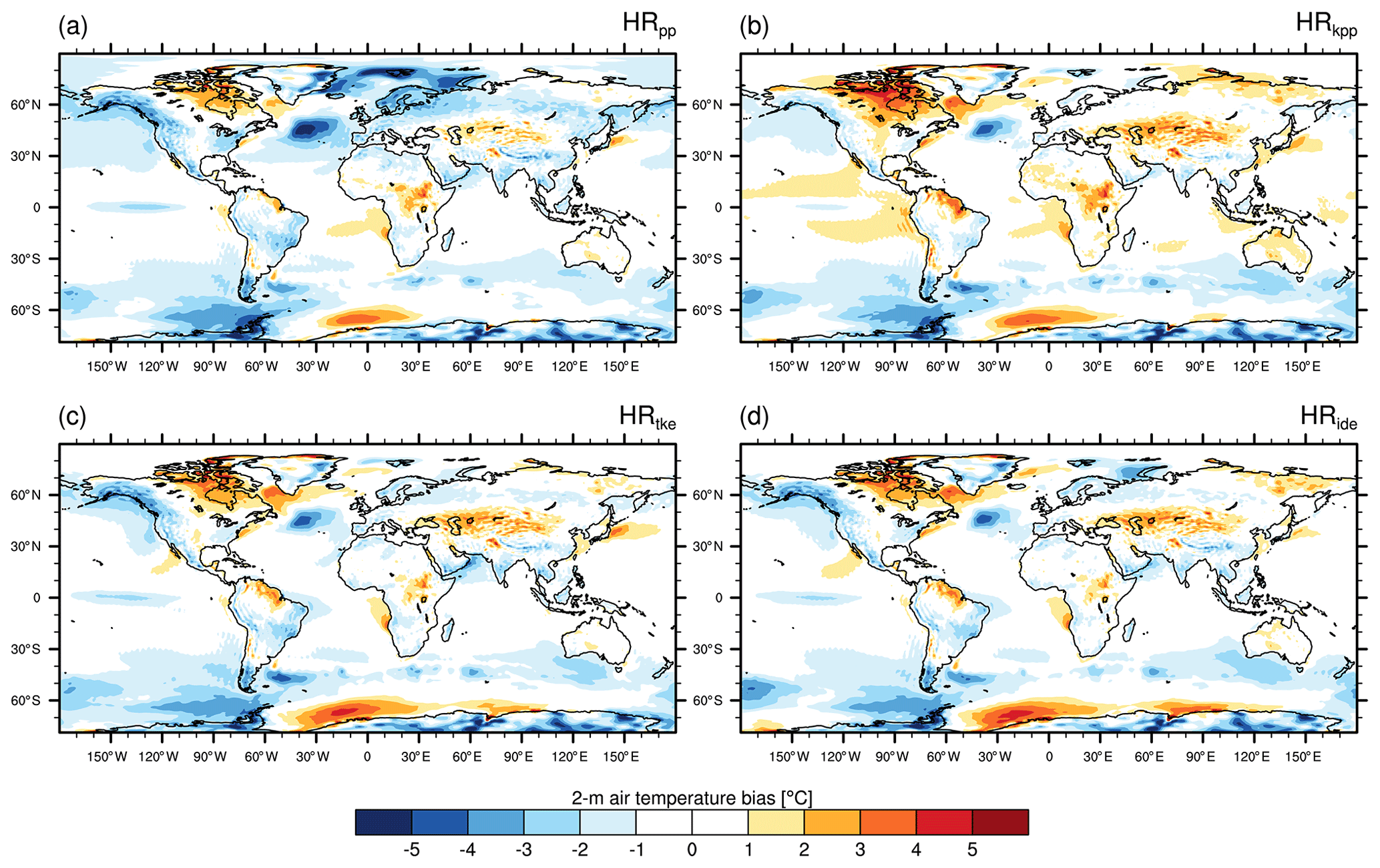
Figure 17 Time-averaged 2 m air temperature (SAT) bias (MPI-ESM1.2 minus EN4) for (a) HR_pp, (b) HR_kpp, (c) HR_tke, and (d) HR_ide.

In the Southern Ocean, the SAT is too cold along the ACC by about 1 ^∘C and colder to the west of the Antarctic peninsula. The air temperature above the Weddell Sea is warmer than in ERA-Interim, especially when using TKE, because of the large sensible heat fluxes from the Weddell Sea polynya. However, even though IDEMIX reduces the area and intensity of this polynya, there is no effect on the SAT, which requires further investigation in a future study.

Other quantities, such as wind speed or precipitation, are not affected by changing the vertical mixing scheme in the ocean.

5.2 Zonal temperature and velocity

The zonally averaged global air temperature is mostly too cold (Fig. 18) in the entire troposphere and too warm in the stratosphere compared to ERA-Interim. Warmer SSTs in the Northern Hemisphere with KPP and TKE(+IDEMIX) propagate to higher layers of the troposphere. While warmer temperatures remain limited to the extratropics of the Northern Hemisphere in HR_tke in comparison to HR_pp (significant at the 5 % level), also the tropics and the Southern Hemisphere become warmer with KPP, which produces also the warmest troposphere.

Figure 18 Time-averaged zonal air temperature bias (MPI-ESM1.2 minus EN4) for (a) HR_pp, (b) HR_kpp, (c) HR_tke, and (d) HR_ide. Stippling in panels (a)–(c) shows where the difference to HR_pp is significant at α=5 % based on adjusted p values with the false discovery rate (FDR) method (Benjamini and Hochberg, 1995) using α_FDR=5 % to account for multiplicity.

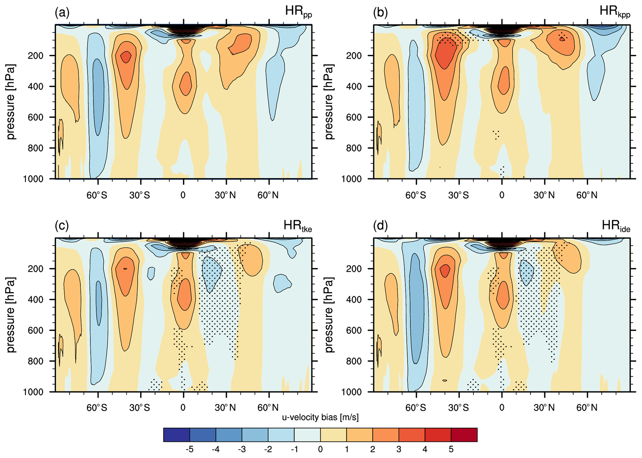
Figure 19 Time-averaged zonal wind speed bias (MPI-ESM1.2 minus EN4) for (a) HR_pp, (b) HR_kpp, (c) HR_tke, and (d) HR_ide. Stippling in panels (a)–(c) shows where the difference to HR_pp is significant at α=5 % based on adjusted p values with the FDR method (Benjamini and Hochberg, 1995) using α_FDR=5 % to account for multiplicity.

The warmer extratropics with TKE result in a weaker meridional gradient that reduces the thermal wind and leads to a weaker jet stream in the Northern Hemisphere (Fig. 19c–d). However, in HR_kpp (Fig. 19b), no weakening of the Northern Hemisphere jet stream is seen, most likely because meridional gradients are maintained when the entire hemisphere is uniformly warmer.

6 Conclusions

We have compared the effect of four different ocean vertical mixing schemes (PP, KPP, TKE, TKE+IDEMIX) on the climate state in MPI-ESM1.2-HR simulations. The ocean mixing library CVMix (Griffies et al., 2015), which we extended with the TKE and TKE+IDEMIX schemes, allowed for a side-by-side comparison of these schemes.

From the results described above, a consistent picture emerges. Using KPP or TKE increases the convection in the SPNA and Nordic Seas but also in the Southern Hemisphere. Due to enhanced convection, the overflows from the Nordic Seas increase by about 10 %. Stronger overflows and increased inflow from the Indian Ocean into the South Atlantic result in a stronger and deeper upper cell of the AMOC. The roughly 3 Sv (or 20 %) stronger AMOC transports more heat and salt into the SPNA and its marginal seas. The higher salinity favours deep convection, maintaining a stronger AMOC, whereas the higher heat transport increases the SSTs. The warmer SSTs affect the atmosphere, resulting in warmer extratropics with TKE, weakening the meridional temperature gradient and thus the jet stream in the Northern Hemisphere. With KPP, the tropics and the Southern Hemisphere also become warmer but without weakening of the jet stream due to a more uniform warming. These results highlight the clear advantage of using coupled models in which the surface state can evolve interactively, rather than air temperature or salinity being dictated by restoring as in ocean-only configurations.

KPP, TKE, and TKE+IDEMIX produce similar results but differ in some aspects. Most pronounced is that IDEMIX produces a more heterogeneous spatial pattern of vertical diffusivity, with generally lower values in deep and flat basins and increased turbulence over rough topography. This spatial pattern is particularly evident in the Arctic Ocean and fits better with microstructure measurements without having to artificially lower the background diffusivity.

In addition, IDEMIX improves the circulation and mixing in the Nordic Seas and the Fram Strait, which reduces the warm bias of the Atlantic Water layer in the Arctic Ocean. In the Southern Hemisphere, IDEMIX reduces the spurious deep convection in the Weddell Sea because of enhanced mixing above the shelf that seems to increase the lateral transport of freshwater into the inner Weddell Sea, thereby impeding deep convection. The main advantages of IDEMIX are its energetically more consistent formulation without assuming an artificial background diffusivity and its flexibility that allows additional energy inputs, e.g. from the mesoscale eddy field.

Appendix A: Ocean vertical mixing schemes in MPI-ESM1.2

In this section, we give a brief summary of the ocean vertical schemes that we have implemented into MPI-ESM1.2. The vertical mixing schemes were implemented via the Community Vertical Mixing (CVMix) library (Griffies et al., 2015; Van Roekel et al., 2018), except for the PP scheme. The KPP schema was already part of the CVMix library, which we therefore extended with the TKE and IDEMIX scheme. This extension will become part of the official CVMix library.

The schemes below aim to parameterize the vertical turbulent fluxes following this general flux-gradient or K-profile approach:

$$\begin{array}{}\text{(A1)}& \stackrel{\mathrm{‾}}{w^{\prime }{\mathit{\lambda }}^{\prime }}=-K_{\mathit{\lambda }}\left({\displaystyle \frac{\partial \mathrm{\Lambda }}{\partial z}}\right)+{\mathrm{\Gamma }}_{\mathit{\lambda }},\end{array}$$

with w^′ the vertical turbulent velocity, λ^′ the turbulent fluctuation of a quantity, λ a grid-scale quantity and the turbulent exchange coefficient (K_λ>0) or also termed eddy viscosity for momentum flux and eddy diffusivity for tracer fluxes, such as temperature or salinity. Γ_λ represents any flux not proportional to the local gradient ∂_zΛ and is referred to as “non-local flux”. In our comparison, Γ_λ is only accounted for in the KPP scheme (Appendix A2).

A1 Pacanowski and Philander (1981, PP) scheme

In our control simulation, the vertical turbulent diffusion and viscosity are based on a modified version of the Richardson-number-dependent formulation by Pacanowski and Philander (1981) (PP) scheme. The modifications are that (1) the vertical diffusivity is not dependent on the vertical viscosity, and (2) that the turbulent mixing in the ocean mixed layer is assumed to depend on the cube of the 10 m wind speed (Marsland et al., 2003). This dependency decays exponentially with depth and with potential density difference to the surface. Since the classical approach by Pacanowski and Philander (1981) underestimates the turbulent mixing close to the surface (Marsland et al., 2003), this additional wind induced mixing (κ_w) is added and defined as

$$\begin{array}{}\text{(A2)}& {\displaystyle }{K}_{\mathrm{w}}\left(\mathrm{1}\right)& {\displaystyle }=(\mathrm{1}-A{)}^{\mathrm{2}}{w}_t{U}_{\mathrm{10}}^{\mathrm{3}}\text{(A3)}& {\displaystyle }{K}_{\mathrm{w}}\left(k\right)& {\displaystyle }=K_{\mathrm{w}}(k-\mathrm{1}){\displaystyle \frac{\frac{\mathit{\lambda }}{\mathrm{\Delta }z}}{\frac{\mathit{\lambda }}{\mathrm{\Delta }z}+{\mathit{\delta }}_z\mathit{\rho }}}{e}^{\frac{\mathit{\lambda }}{z_{\mathrm{0}}}},\end{array}$$

with $k=\mathrm{2},\mathrm{3},\mathrm{\dots },n$ the vertical model level, Δz the layer thickness, A the fractional sea ice concentration, U₁₀ the 10 m wind speed, $w_t=\mathrm{0.5}\times {\mathrm{10}}^{-\mathrm{3}}/{\mathrm{6.0}}^{\mathrm{3}}$, λ=0.03, and z₀=40.0 (e-folding depth) are adjustable parameters, and δ_zρ the local static stability.

The total equation for the eddy vertical diffusivity then reads

$$\begin{array}{}\text{(A4)}& K_d\left(z\right)={\displaystyle \frac{d_{v,\mathrm{0}}}{\left(\mathrm{1}+c_{d}Ri(z{)}^{\mathrm{2}}\right)}}+K_{\mathrm{w}}\left(z\right)+d_{v,\mathrm{b}},\end{array}$$

with $d_{v,\mathrm{0}}=\mathrm{0.2}\times {\mathrm{10}}^{-\mathrm{2}}$ m² s⁻¹, c_d=5.0, and the background diffusivity $d_{v,\mathrm{b}}=\mathrm{5}\times {\mathrm{10}}^{-\mathrm{5}}$ m² s⁻¹. The eddy vertical viscosity is parameterized as

$$\begin{array}{}\text{(A5)}& K_v\left(z\right)={\displaystyle \frac{a_{v,\mathrm{0}}}{\left(\mathrm{1}+c_{a}Ri(z{)}^{\mathrm{3}}\right)}}+K_{\mathrm{w}}\left(z\right)+a_{v,b},\end{array}$$

with $a_{v,\mathrm{0}}=\mathrm{0.2}\times {\mathrm{10}}^{-\mathrm{2}}$ m² s⁻¹, c_a=5.0, and $a_{v,\mathrm{b}}=\mathrm{1.05}\times {\mathrm{10}}^{-\mathrm{5}}$ m² s⁻¹ the background viscosity. The eddy coefficients K_d and K_v are partially relaxed to the value at the previous time step by use of a time filter to avoid 2Δt oscillations (Marsland et al., 2003). Convection is parameterized as enhanced diffusivity (K_d=0.1 m² s⁻¹) for the PP scheme.

Table A1 Resulting p values from Welch's two-sided t tests (α=0.05 and n=20) for testing the differences in mean overflow volumes of DSOW, in the FSC, and in the FBC.

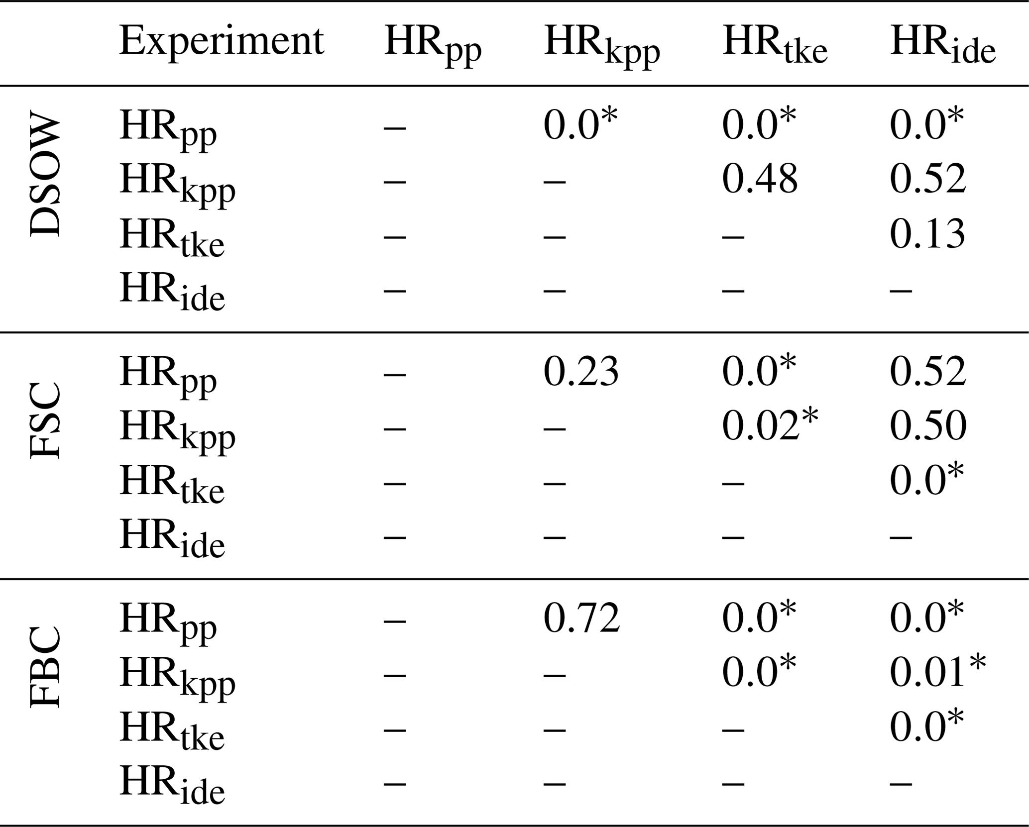
^* Significant at level α. To achieve a power (1-β) of 80 % with n=20 and α=0.05, the minimum effect size $d=\left|{\mathit{\mu }}_{\mathrm{1}}-{\mathit{\mu }}_{\mathrm{2}}\right|/\sqrt{({\mathrm{SD}}_{\mathrm{1}}^{\mathrm{2}}+{\mathrm{SD}}_{\mathrm{2}}^{\mathrm{2}})/\mathrm{2}}$ is about 1.0. For instance, a pooled standard deviation of, e.g. 0.1 Sv would correspond to a minimum mean difference of $\left|{\mathit{\mu }}_{\mathrm{1}}-{\mathit{\mu }}_{\mathrm{2}}\right|=\mathrm{0.1}$ Sv.

A2 KPP scheme

The second simulation uses the KPP scheme from Large et al. (1994) for the mixed layer. In general, a turbulent flux ($\stackrel{\mathrm{‾}}{w^{\prime }{\mathit{\lambda }}^{\prime }}=\stackrel{\mathrm{‾}}{w\mathit{\lambda }}$) of a quantity Λ (momentum, scalar tracers) is parameterized as

$$\begin{array}{}\text{(A6)}& \stackrel{\mathrm{‾}}{w\mathit{\lambda }}=-K_{\mathit{\lambda }}\left({\displaystyle \frac{\partial \mathrm{\Lambda }}{\partial z}}\right)+K_{\mathit{\lambda }}^{\text{non-local}}{\mathit{\gamma }}_{\mathit{\lambda }},\end{array}$$

with K_λ the local diffusivity for tracers or viscosity for momentum, z the depth, $K_{\mathit{\lambda }}^{\text{non-local}}$ the non-local diffusivity or viscosity, and a non-local term γ_λ. While the local flux (first term on the right-hand side) depends directly on the local gradient of a quantity, the non-local flux (second term on the right-hand side) redistributes the surface fluxes throughout the whole surface boundary layer, for example, due to convection (see below).

The local diffusivity (K_λ) is calculated as

$$\begin{array}{}\text{(A7)}& K_{\mathit{\lambda }}\left(\mathit{\sigma }\right)=h{w}_{\mathit{\lambda }}\left(\mathit{\sigma }\right)G\left(\mathit{\sigma }\right),\end{array}$$

with $\mathit{\sigma }=z/h$ the dimensionless vertical coordinate ($\mathrm{0}\le \mathit{\sigma }\le \mathrm{1}$), z the depth below the sea surface, h the ocean boundary layer depth, w_λ a vertical turbulent velocity scale (either for scalar tracers or momentum), and $G\left(\mathit{\sigma }\right)=\mathit{\sigma }(\mathrm{1}-\mathit{\sigma }{)}^{\mathrm{2}}$ a universal shape function. Oftentimes, and also in our implementation, it is assumed that $K_{\mathit{\lambda }}^{\text{non-local}}=K_{\mathit{\lambda }}$ (Griffies et al., 2015).

The ocean boundary layer depth h is determined at the depth z where the bulk Richardson number Ri_b becomes larger than a critical Richardson number Ri_c=0.3. The bulk Richardson number at depth z is defined as

$$\begin{array}{}\text{(A8)}& R{i}_{\mathrm{b}}\left(z\right)={\displaystyle \frac{\left(z-z_{\mathrm{sl}}\right)\left[B_{\mathrm{sl}}-B\left(z\right)\right]}{{\left|{\mathit{U}}_{\mathrm{sl}}-\mathit{U}\left(z\right)\right|}^{\mathrm{2}}+U_{\mathrm{t}}(z{)}^{\mathrm{2}}}},\end{array}$$

with z_sl the depth at the centre of the surface layer (defined as $\mathrm{0}\le z\le \mathit{ϵ}h$), where we assume that the surface layer is 10 % (ϵ=0.1) of the ocean boundary layer depth h, as in Large et al. (1994). Since the calculation of the ocean boundary layer depth h requires Ri_b, which itself requires h, we face a cyclic problem. To solve this problem, we follow the column sampling method recommended by Griffies et al. (2015) (see details in their description).

B_sl is the surface layer averaged buoyancy flux, B(z) the local buoyancy flux, U_sl the surface layer averaged velocity, U(z) the local velocity, and U_t(z) a parameterization for unresolved turbulent vertical velocity shear that reduces the bulk Richardson number (see, e.g. Griffies et al., 2015, for the definition of the unresolved turbulent shear).

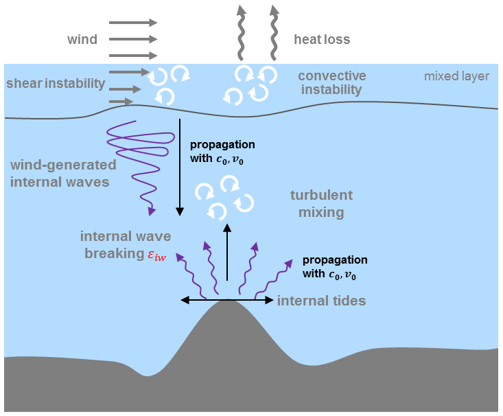
Figure A1 Schematic of the combined TKE+IDEMIX scheme used in HR_ide. For processes parameterized in TKE, away from strong currents, shear and buoyancy instability (convection) are largest near the surface (grey arrows), causing strong mixing in the mixed layer (white eddy symbols). For processes parameterized by IDEMIX, below the mixed layer, internal waves are either induced by fluctuating wind stress or by interactions of barotropic tides with orographic features (violet arrows). The internal waves are propagating into the interior ocean (black arrows), where they eventually break and dissipate (white eddy symbols).

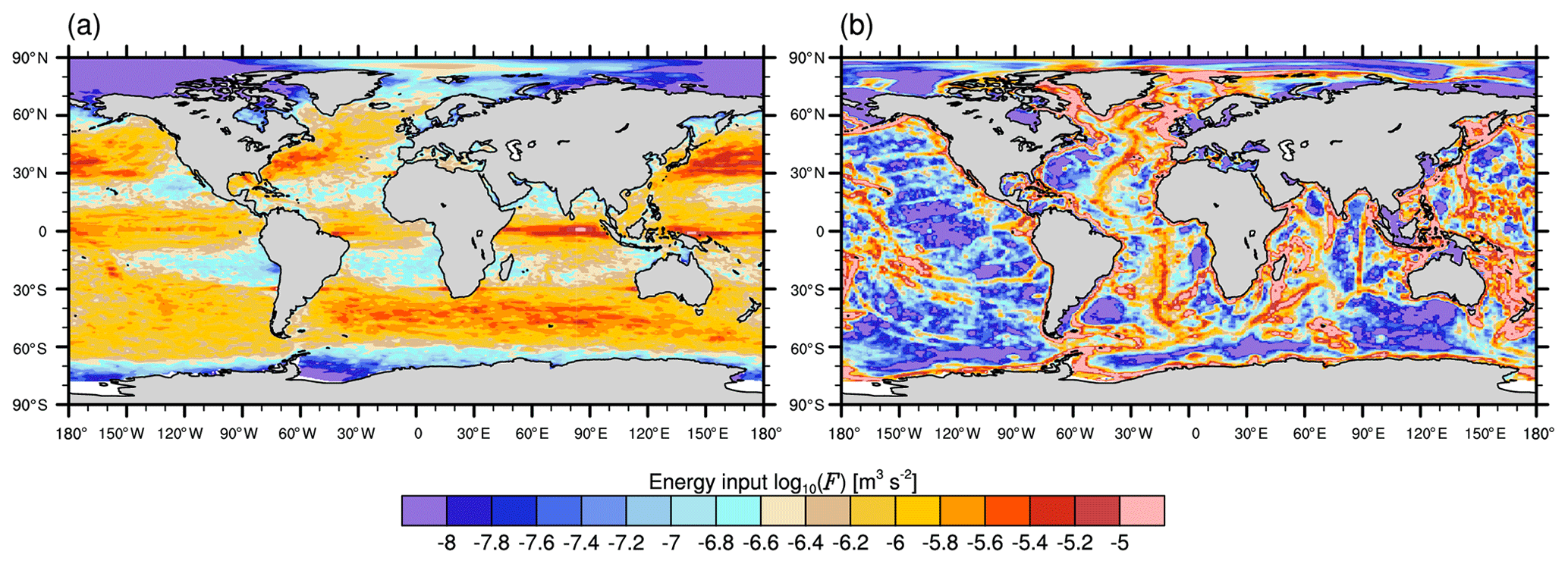
Figure A2 Energy input log ₁₀(F) (m³ s⁻³) at (a) the surface by near-inertial waves from Rimac et al. (2013) and (b) by tidal forcing at the ocean bottom from Jayne (2009).

The vertical turbulent velocity scale w_λ is calculated as follows:

$$\begin{array}{}\text{(A9)}& w_{\mathit{\lambda }}\left(\mathit{\sigma }\right)={\displaystyle \frac{\mathit{\kappa }{u}_{*}(\mathrm{1}-A{)}^{\mathrm{2}}}{{\mathrm{\Phi }}_{\mathrm{\Lambda }}\left(\mathit{\zeta }\right)}},\end{array}$$

with κ=0.4 the von Kármán constant, u_* the surface friction velocity that reduces with increasing fractional sea ice (A), Φ_Λ a dimensionless similarity function (momentum or scalar tracer), depending on $\mathit{\zeta }=\mathit{\sigma }h/L$, with $L=\frac{u_{*}^{\mathrm{3}}}{\mathit{\kappa }{B}_{\mathrm{f}}}$ the Monin–Obukhov length scale. B_f is the buoyancy forcing in the ocean boundary layer. Under neutral forcing ($\mathit{\zeta }=\mathrm{0}\to {\mathrm{\Phi }}_{\mathrm{\Lambda }}\left(\mathrm{0}\right)=\mathrm{1}$), Eq. (A9) reduces to $w_{\mathit{\lambda }}\left(\mathit{\sigma }\right)=\mathit{\kappa }{u}_{*}(\mathrm{1}-A{)}^{\mathrm{2}}$. We use the similarity functions of Large et al. (1994) (see Appendix B) for stable (ζ>0), unstable (${\mathit{\zeta }}_{\mathrm{m}}<\mathit{\zeta }<\mathrm{0}$ or ${\mathit{\zeta }}_{\mathrm{s}}<\mathit{\zeta }<\mathrm{0}$), and very unstable conditions (ζ<0):

$$\begin{array}{}\text{(A10)}& {\displaystyle }{\mathrm{\Phi }}_{\mathrm{m}}\left(\mathit{\zeta }\right)=& {\displaystyle }\left\{\begin{array}{ll}\mathrm{1}+\mathrm{5}\mathit{\zeta }& \mathit{\zeta }>\mathrm{0}\\ (\mathrm{1}-\mathrm{16}\mathit{\zeta }{)}^{-\mathrm{1}/\mathrm{4}}& {\mathit{\zeta }}_{\mathrm{m}}<\mathit{\zeta }<\mathrm{0}\\ (a_{\mathrm{m}}-c_{\mathrm{m}}\mathit{\zeta }{)}^{-\mathrm{1}/\mathrm{3}}& \mathit{\zeta }<-{\mathit{\zeta }}_{\mathrm{m}}\end{array}\right.\text{(A11)}& {\displaystyle }{\mathrm{\Phi }}_{\mathrm{s}}\left(\mathit{\zeta }\right)=& {\displaystyle }\left\{\begin{array}{ll}\mathrm{1}+\mathrm{5}\mathit{\zeta }& \mathit{\zeta }>\mathrm{0}\\ (\mathrm{1}-\mathrm{16}\mathit{\zeta }{)}^{-\mathrm{1}/\mathrm{4}}& {\mathit{\zeta }}_{\mathrm{s}}<\mathit{\zeta }<\mathrm{0}\\ (a_{\mathrm{s}}-c_{\mathrm{s}}\mathit{\zeta }{)}^{-\mathrm{1}/\mathrm{3}}& \mathit{\zeta }<{\mathit{\zeta }}_{\mathrm{s}},\end{array}\right.\end{array}$$

with ${\mathit{\zeta }}_{\mathrm{m}}=-\mathrm{0.2}$, ${\mathit{\zeta }}_{\mathrm{s}}=-\mathrm{1.0}$, a_m=1.26, c_m=8.38, $a_{\mathrm{s}}=-\mathrm{28.86}$, and c_s=98.96. We do not match the diffusivities at the base of the mixed layer to avoid overshooting tracers, as recommended by Griffies et al. (2015).

For the non-local flux term in Eq. (A6), it is assumed that $K_{\mathit{\lambda }}=K_{\mathit{\lambda }}^{\text{non-local}}$, so that this term simplifies to K_λγ_λ. The non-local flux γ_λ is only non-zero if B_f<0 (buoyancy gain at the surface) and only for scalar tracers such as temperature, θ, or salinity, s; for momentum it is set to zero. With the assumption $K_{\mathit{\lambda }}=K_{\mathit{\theta }}=K_{\mathrm{s}}$ and a universal shape function (G(σ)), the non-local fluxes take the form

$$\begin{array}{}\text{(A12)}& {\displaystyle }{\stackrel{\mathrm{‾}}{w\mathit{\theta }}}^{\text{non-local}}& {\displaystyle }=K_{\mathit{\lambda }}{\mathit{\gamma }}_{\mathit{\theta }}=-G\left(\mathit{\sigma }\right)C_{\mathrm{s}}\left({\displaystyle \frac{Q^{\text{heat}}}{{\mathit{\rho }}_{\mathrm{0}}{C}_P^{\mathrm{0}}}}\right)\text{(A13)}& {\displaystyle }{\stackrel{\mathrm{‾}}{ws}}^{\text{non-local}}& {\displaystyle }=K_{\mathit{\lambda }}{\mathit{\gamma }}_{\mathrm{s}}=-G\left(\mathit{\sigma }\right)C_s{Q}^s,\end{array}$$

with the non-local terms for temperature (γ_θ) and salinity (γ_s), a dimensionless coefficient $C_{\mathrm{s}}=C_{*}\mathit{\kappa }(c_{\mathrm{s}}\mathit{\kappa }\mathit{ϵ}{)}^{\mathrm{1}/\mathrm{3}}$ with a dimensionless constant $C_{*}=\mathrm{10}$, ρ₀=1025 kg m⁻³ the reference seawater density, $C_P^{\mathrm{0}}$ the seawater heat capacity at constant pressure ($\mathrm{J}{\mathrm{kg}}^{-\mathrm{1}}{}^{\circ }{\mathrm{C}}^{-\mathrm{1}}$), Q_s the mass flux of salt ($\mathrm{kg}{\mathrm{m}}^{-\mathrm{2}}{\mathrm{s}}^{-\mathrm{1}}$), and the heat flux Q^heat (W m⁻²) that considers penetrative shortwave radiation. See further details on the KPP scheme in Griffies et al. (2015) and Van Roekel et al. (2018).

Below the mixed layer, we use the PP scheme with the enhanced diffusivity parameterization for convection, as described in Appendix A1.

A3 TKE and IDEMIX schemes

A schematic overview of the TKE and IDEMIX schemes are depicted in Fig. A1. IDEMIX parameterizes the internal wave energy (E_iw) in terms of a budget equation:

$$\begin{array}{}\text{(A14)}& {\displaystyle \frac{\partial E_{\mathrm{iw}}}{\partial t}}={\mathrm{\nabla }}_h{\mathit{\nu }}_{\mathrm{0}}{\mathit{\tau }}_h{\mathrm{\nabla }}_h{\mathit{\nu }}_{\mathrm{0}}{E}_{\mathrm{iw}}+{\displaystyle \frac{\partial }{\partial z}}\left(c_{\mathrm{0}}{\mathit{\tau }}_v{\displaystyle \frac{\partial c_{\mathrm{0}}{E}_{\mathrm{iw}}}{\partial z}}\right)-{\mathit{ϵ}}_{\mathrm{iw}},\end{array}$$

with ν₀ the lateral group velocity, τ_h a lateral timescale on which lateral anisotropies are eliminated by non-linear wave–wave interactions, c₀ the weighted average vertical group velocity, z the vertical coordinate, τ_v a timescale on the order of days, and ${\mathit{ϵ}}_{\mathrm{iw}}=-\mathit{\alpha }{E}_{\mathrm{iw}}^{\mathrm{2}}$ the dissipation of internal wave energy, with α a structure function depending on the stratification (for details, see Olbers and Eden, 2013). The first and second terms on the right-hand side (RHS) parameterize the horizontal and vertical propagation of internal waves, respectively. Internal wave energy is dissipated by the last term on the RHS of Eq. (A14). This term acts as an energy transfer from internal wave energy to turbulent kinetic energy (see Eq. A15 below).

Internal waves are forced in IDEMIX by surface and bottom fluxes applied as boundary conditions in the second term on the RHS of Eq. (A14). Currently, we use time-constant fields for the energy fluxes at the surface and at the bottom (see Fig. A2), as in Eden et al. (2014). The energy flux that we use as surface boundary condition is 20 % of the wind input into the inertial band of the mixed layer (Jochum et al., 2013), as determined by Rimac et al. (2013) (inertial pumping mechanism). We neglect, however, other sources exciting internal waves near the surface, for instance, buoyancy plumes that overshoot the mixed layer base, vertical roll vortices of turbulent eddies, or Langmuir circulation that undulates internal waves (Czeschel and Eden, 2019). At the bottom, barotropic tides interact with the bottom roughness and convert energy to internal waves. This energy flux is prescribed from Jayne (2009), with the constraint that this energy source is not flow aware.

In commonly used vertical mixing schemes, such as KPP (Large et al., 1994) or TKE (Gaspar et al., 1990), the breaking of internal waves is usually parameterized by simply assuming a constant background diffusivity (either a scalar or profile) or constant background TKE value. By using TKE with IDEMIX, the constant background diffusivity is replaced by one that is diagnosed from the internal wave energy using the Osborn–Cox relation. We use the recommended parameter set from Pollmann et al. (2017), who compared TKE coupled to IDEMIX with Argo float data in stand-alone ocean simulations.

The modified TKE equation (Eden et al., 2014) then reads

$$\begin{array}{}\text{(A15)}& \begin{array}{rl}& {\displaystyle \frac{\mathrm{d}{\overline{E}}_{\mathrm{tke}}}{\mathrm{d}t}}=-{\partial }_z\left(\mathrm{fluxes}\right)+c_{u}K\left({\partial }_z{\overline{\mathit{u}}}^{\mathrm{2}}\right)\\ & -c_{b}K{N}^{\mathrm{2}}-{\mathit{ϵ}}_{\mathrm{tke}}+{\mathit{ϵ}}_{\mathrm{iw}},\end{array}\end{array}$$

with the dimensionless parameters c_u and c_b, which are related by $c_u=c_b{R}_i/R_f$. The first term on the RHS describes the redistribution of TKE in the vertical. Surface fluxes enter as boundary conditions to this term. The second term describes the vertical momentum fluxes acting on the shear of the mean flow, transferring energy from the mean flow to TKE. The third term is the buoyancy term that transfers energy to the potential energy of the mean flow, thereby decreasing TKE. The dissipation of TKE (fourth term) is parameterized as ${\mathit{ϵ}}_{\mathrm{tke}}={\overline{E}}_{\mathrm{tke}}^{\mathrm{2}/\mathrm{3}}{L}^{-\mathrm{1}}$ with the mixing length $L=\sqrt{\mathrm{2}{\overline{E}}_{\mathrm{tke}}/N^{\mathrm{2}}}$ (Blanke and Delecluse, 1993; Eden et al., 2014). The last term on the RHS is then the new contribution from IDEMIX, which is absent when using TKE without IDEMIX.

The diffusivity is parameterized as $K={\overline{E}}_{\mathrm{tke}}^{\mathrm{1}/\mathrm{2}}L$ by assuming the same mixing length as for the dissipation. If TKE is used alone without being combined with IDEMIX, then a background diffusivity is assumed to represent internal wave breaking (Eden et al., 2014). When TKE is used alone without being coupled to IDEMIX, the turbulent kinetic energy is set to a background value of $E_{\min }={\mathrm{10}}^{-\mathrm{6}}$ m²s⁻². The corresponding diffusivity in this case reads $K=\sqrt{\mathrm{2}}{c}_b{E}_{min}/N$.