MESMO 3: Flexible phytoplankton stoichiometry and refractory dissolved organic matter

We describe the third version of Minnesota Earth System Model for Ocean biogeochemistry (MESMO 3), an Earth system model of intermediate complexity, with a dynamical ocean, dynamic–thermodynamic sea ice, and an energy–moisture-balanced atmosphere. A major feature of version 3 is the flexible $\mathrm{C}:\mathrm{N}:\mathrm{P}$ ratio for the three phytoplankton functional types represented in the model. The flexible stoichiometry is based on the power law formulation with environmental dependence on phosphate, nitrate, temperature, and light. Other new features include nitrogen fixation, water column denitrification, oxygen and temperature-dependent organic matter remineralization, and CaCO₃ production based on the concept of the residual nitrate potential growth. In addition, we describe the semi-labile and refractory dissolved organic pools of C, N, P, and Fe that can be enabled in MESMO 3 as an optional feature. The refractory dissolved organic matter can be degraded by photodegradation at the surface and hydrothermal vent degradation at the bottom. These improvements provide a basis for using MESMO 3 in further investigations of the global marine carbon cycle to changes in the environmental conditions of the past, present, and future.

1 Introduction

Here we document the development of the third version of the Minnesota Earth System Model for Ocean biogeochemistry (MESMO 3). As described for the first two versions (Matsumoto et al., 2008, 2013), MESMO is based on the non-modular version of the Grid ENabled Integrated Earth (GENIE) system model (Lenton et al., 2006; Ridgwell et al., 2007). The computationally efficient ocean–climate model of Edwards and Marsh (Edwards and Marsh, 2005) forms the core of GENIE's physical model. MESMO is an Earth system model of intermediate complexity (EMIC), which occupies a midpoint in the continuum of climate models that span high-resolution, comprehensive coupled models on one end and box models on the other (Claussen et al., 2002). MESMO has a 3D dynamical ocean model on a 36 × 36 equal-area horizontal grid with 10^∘ increments in longitude and uniform in the sine of latitude. There are 16 vertical levels. It is coupled to a 2D energy moisture-balanced model of the atmosphere and a 2D dynamic and thermodynamic model of sea ice. Thus, MESMO retains important dynamics that allow for simulations of transient climate change, while still being computationally efficient.

Since the first version, MESMO has continued to be developed chiefly for investigations of ocean biogeochemistry (Table 1). Briefly, in MESMO 1 the main improvements over the predecessor GENIE focused on the biological production and remineralization, as well as on the uptake of natural radiocarbon (¹⁴C) and anthropogenic transient tracers (Matsumoto et al., 2008). The net primary production (NPP) in MESMO 1 occurred in the top two vertical levels, representing the surface 100 m, and depended on temperature, nutrients, light, and mixed-layer depth (MLD). The nutrient dependence was based on the Michaelis–Menten uptake kinetics of phosphate (PO₄), nitrate (NO₃), and aqueous CO₂. The limiting nutrient was determined by Liebig's rule of the minimum relative to the fixed uptake stoichiometry of $\mathrm{C}:\mathrm{N}:\mathrm{P}=\mathrm{117}:\mathrm{16}:\mathrm{1}$. A single generic phytoplankton functional type (PFT) carried out NPP, which was split between particulate organic matter (POM) and dissolved organic matter (DOM) in a globally constant ratio of 1:2. The semi-labile form of the dissolved organic carbon (DOC) was the only form of DOM simulated in MESMO 1. The POM flux across the 100 m level defined the export production. The vertical flux of POM was driven by a fixed rate of sinking and a temperature-dependent, variable remineralization rate.

Table 1 Summary of MESMO development.

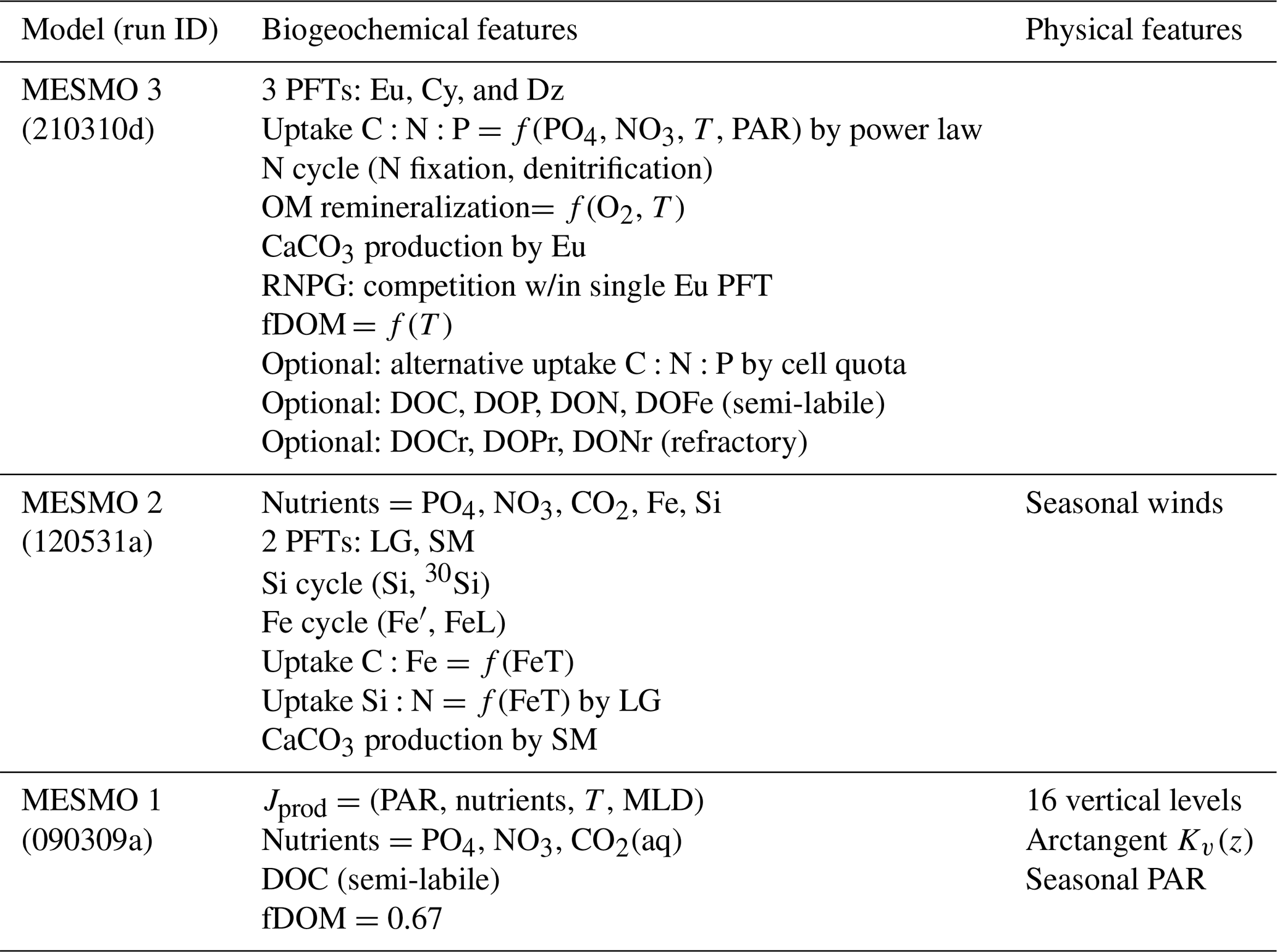
PFT stands for phytoplankton functional types. MESMO 2 PFTs are as follows: LG stands for large (diatoms) and SM stands for small. MESMO 3 PFTs are as follows: Eu stands for eukaryotes, Cy stands for cyanobacteria, and Dz stands for diazotrophs. OM stands for organic matter. RNPG stands for residual nitrate potential growth. T stands for temperature. PAR stands for photosynthetically available radiation. fDOM stands for the fraction of NPP routed to dissolved organic matter (DOM). The two types of DOM are semi-labile (DOC, DOP, DON, and DOFe) and refractory (DOCr, DOPr, and DONr). Carbon isotopes (¹²C, ¹³C, and ¹⁴C) are calculated separately for DOC and DOCr. The run ID is 210310m for the MESMO 3 experiment LVR and 210310o for the experiment LVR with fDOM_r=0.2 %.

The main aim of MESMO 2 was a credible representation of the marine silica cycle (Matsumoto et al., 2013). To this end, the set of limiting nutrients (P, N, and C) in MESMO 1 was augmented to include iron (Fe) and silicic acid (Si(OH)₄) in MESMO 2 (Table 1). The stable isotope of Si (³⁰Si) was also added as a state variable. The Fe cycle included an aeolian flux of Fe, complexation with organic ligand, and particle scavenging of free Fe. The scavenged Fe that reached the seafloor was removed from the model domain. This burial flux of Fe balanced the aeolian flux at steady state. In addition, a new PFT was added in MESMO 2 chiefly to represent diatoms. This new “large” PFT was limited by Si and characterized by a high maximum growth rate and large half-saturation constants for the nutrient uptake kinetics. It represented fast and opportunistic phytoplankton that do well under nutrient replete conditions. In comparison, the “small” PFT was characterized by a lower maximum growth rate and smaller half-saturation constants and outperformed the large PFT in oligotrophic subtropical gyres. CaCO₃ production was associated with the “small” PFT in MESMO 2. The addition of Fe, Si, and the large PFT in MESMO 2 allowed it to have a Fe-dependent, variable Si:N uptake ratio (Hutchins and Bruland, 1998; Takeda, 1998), which is critical for simulating important features of the global ocean Si distribution.

MESMO 1 and 2 were assessed and calibrated by multi-objective tuning and extensive model–data comparisons of transient tracers (anthropogenic carbon, CFCs), deep ocean Δ¹⁴C, and nutrients (Matsumoto et al., 2008, 2013). These versions have been employed successfully in a number of studies of global distributions of carbon and carbon isotopes under various conditions of the past, present, and future (Cheng et al., 2018; Lee et al., 2011; Matsumoto et al., 2010, 2020; Matsumoto and McNeil, 2012; Matsumoto and Yokoyama, 2013; Sun and Matsumoto, 2010; Tanioka and Matsumoto, 2017; Ushie and Matsumoto, 2012). In addition, MESMO 1 and 2 have participated in model intercomparison projects (Archer et al., 2009; Cao et al., 2009; Eby et al., 2013; Joos et al., 2013; Weaver et al., 2012; Zickfeld et al., 2013).

In this contribution, we describe the third and latest version of MESMO with a number of substantial biogeochemical model modifications and new features that bring MESMO up to date with the evolving and accumulating knowledge of the ocean biogeochemical cycle (Table 1). There is no change in the physical model between MESMO 3 and MESMO 2. The most significant new feature of MESMO 3 over the previous versions is the power law formulation of flexible phytoplankton $\mathrm{C}:\mathrm{N}:\mathrm{P}$ ratio. Other new features include additional PFT diazotrophs that carry out N fixation, water column denitrification, the dependence of organic matter remineralization on the dissolved oxygen (O₂) and temperature, and CaCO₃ production based on the concept of the residual nitrate potential growth. In addition, we describe the semi-labile DOM for P, N, and Fe (DOP_sl, DON_sl, and DOFe_sl) and the refractory DOM for C, P, and N (DOC_r, DOP_r, and DON_r), which can be activated as an optional feature in MESMO 3. Some of these features have been described separately in different publications (Matsumoto et al., 2020; Matsumoto and Tanioka, 2020; Tanioka and Matsumoto, 2017, 2020a). This work consolidates the descriptions of all these features in a single publication.

2 Model description

Here we present the full set of biogeochemical equations of MESMO 3 and the key model parameters (Table 2). We describe only the biogeochemical source and sink terms and omit the physical (advective and diffusive) transport terms that are calculated by the ocean circulation model. We discuss the production terms first, followed by remineralization terms, and finally the conservation equations that incorporate both terms.

Table 2 MESMO 3 biogeochemical model parameters values: (a) phytoplankton nutrient uptake; (b) power law model of flexible $\mathrm{C}:\mathrm{N}:\mathrm{P}$ stoichiometry; (c) iron uptake stoichiometry; (d) parameters related to POM, DOM, CaCO₃, and opal; (e) nitrogen and iron cycles.

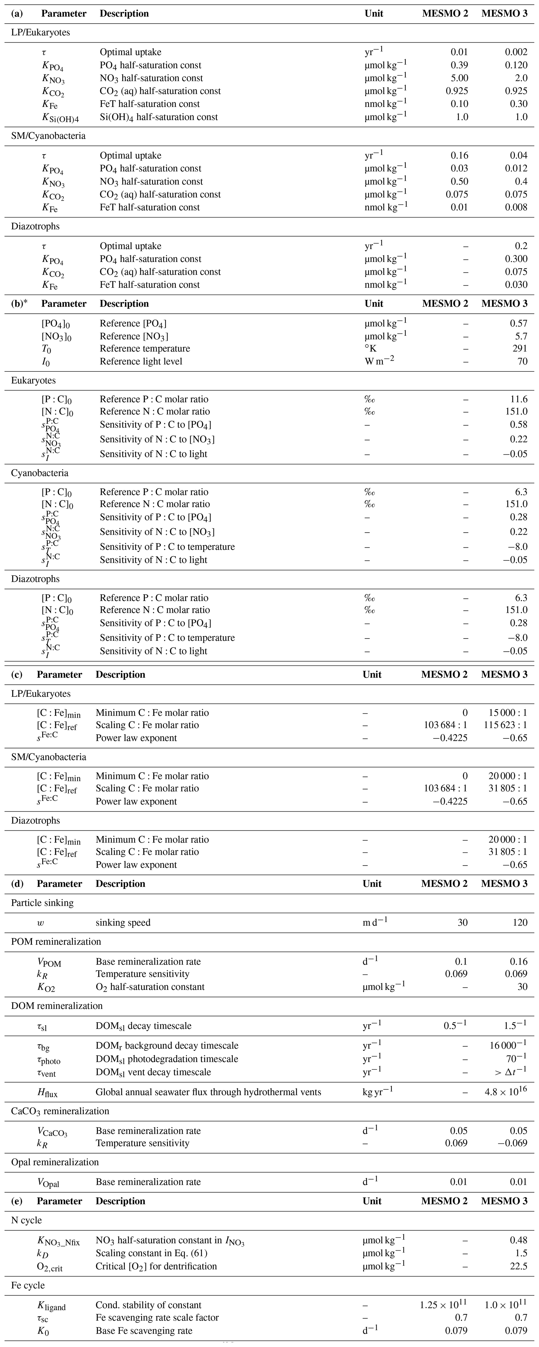
^* Sensitivity factors not listed in Table 2b have a value of zero (e.g., $s_{{\mathrm{PO}}_{\mathrm{4}}}^{\mathrm{N}:\mathrm{C}}=\mathrm{0}$; thus, the environmental driver PO₄ does not drive the N:C ratio). The reference ratios are in ‰ so that [P:C]₀=11.6 ‰ (i.e., C:P = 86.2) for eukaryotes, and [P:C]₀= 6.3 ‰ (i.e., C:P = 158.7) for cyanobacteria and diazotrophs. The reference ratio [N:C]₀= 151.0 ‰ for all PFTs (i.e., $\mathrm{C}:\mathrm{N}:$ = 106:16) is the Redfield ratio.

2.1 Phytoplankton nutrient uptake

NPP occurs in the top two vertical levels of the ocean domain above the fixed compensation depth (z_c) of 100 m. Key parameter values are given in Table 2a. Nutrient uptake by phytoplankton type i (Γ_i) depends on the optimal nutrient uptake timescale (τ_i), nutrients, temperature (T), irradiance (I), and mixed-layer depth (z_ml):

$$\begin{array}{}\text{(1)}& {\mathrm{\Gamma }}_i={\displaystyle \frac{\mathrm{1}}{{\mathit{\tau }}_i}}\cdot F_{\mathrm{N},i}\cdot F_T\cdot F_I\cdot max\left\{\mathrm{1},{\displaystyle \frac{z_{\mathrm{c}}}{z_{\mathrm{ml}}}}\right\}.\end{array}$$

Subscript i refers to PFT (i=1: eukaryotes; i=2: cyanobacteria; i=3: diazotrophs). The nutrient dependence F_N,i is given by Liebig's law of minimum combined with Michaelis–Menten uptake kinetics of limiting nutrients: PO₄, NO₃, CO₂ (aq), total dissolved iron (sum of free iron and ligand-bound iron: FeT = Fe${}^{\prime }+$FeL), and Si(OH)₄:

$$\begin{array}{}\text{(2)}& \begin{array}{rl}& F_{\mathrm{N},i}=min\left({\displaystyle \frac{\left[{\mathrm{PO}}_{\mathrm{4}}\right]}{\left[{\mathrm{PO}}_{\mathrm{4}}\right]+K_{{\mathrm{PO}}_{\mathrm{4}},i}}}\cdot \left[{\mathrm{PO}}_{\mathrm{4}}\right],\right.\\ & {\displaystyle \frac{\left[{\mathrm{NO}}_{\mathrm{3}}\right]}{\left[{\mathrm{NO}}_{\mathrm{3}}\right]+K_{{\mathrm{NO}}_{\mathrm{3}},i}}}\cdot \left[{\mathrm{NO}}_{\mathrm{3}}\right]\cdot Q_{\mathrm{N},i}^{-\mathrm{1}},{\displaystyle \frac{\left[{\mathrm{CO}}_{\mathrm{2}}\left(\mathrm{aq}\right)\right]}{\left[{\mathrm{CO}}_{\mathrm{2}}\left(\mathrm{aq}\right)\right]+K_{{\mathrm{CO}}_{\mathrm{2}},i}}}\\ & \cdot \left[{\mathrm{CO}}_{\mathrm{2}}\left(\mathrm{aq}\right)\right]\cdot Q_{\mathrm{C},i}^{-\mathrm{1}},{\displaystyle \frac{\left[\mathrm{FeT}\right]}{\left[\mathrm{FeT}\right]+K_{\mathrm{FeT},i}}}\cdot \left[\mathrm{FeT}\right]\\ & \left.\cdot Q_{\mathrm{Fe},i}^{-\mathrm{1}},{\displaystyle \frac{\left[\mathrm{Si}{\left(\mathrm{OH}\right)}_{\mathrm{4}}\right]}{\left[\mathrm{Si}{\left(\mathrm{OH}\right)}_{\mathrm{4}}\right]+K_{\mathrm{Si}{\left(\mathrm{OH}\right)}_{\mathrm{4}}}}}\cdot \left[\mathrm{Si}{\left(\mathrm{OH}\right)}_{\mathrm{4}}\right]\cdot Q_{\mathrm{Si}}^{-\mathrm{1}}\right),\end{array}\end{array}$$

where K_X,i is the half-saturation concentration of nutrient X for PFT i. Only eukaryotes (i=1) are limited by Si(OH)₄. Diazotrophs (i=3) are not limited by NO₃. Nutrient uptake Γ is based on the master nutrient variable P, and all other nutrient uptake is related to Γ by the uptake stoichiometry Q_X,i, where X is N, Fe, Si, or C. For example, $Q_{\mathrm{C},i}={\frac{\mathrm{1}}{\left[\mathrm{P}:\mathrm{C}\right]}}_i$ for PFT i. Thus, Q_C,i is numerically equivalent to C:P for PFT i, but we write the equations in terms of P:C for numerical stability and convenience. The Q_X,i ratios represent the flexible phytoplankton uptake stoichiometry and are described more fully in Sect. 2.2.

The temperature dependence F_T of Eq. (1) is given by

$$\begin{array}{}\text{(3)}& F_T={\displaystyle \frac{T\left({}^{\circ }\mathrm{C}\right)+\mathrm{2}}{T\left({}^{\circ }\mathrm{C}\right)+\mathrm{10}}},\end{array}$$

which is analogous to the commonly used Q₁₀=2 relationship. Light limitation F_I of Eq. (1) is described by a hyperbolic function:

$$\begin{array}{}\text{(4)}& F_T={\displaystyle \frac{I}{I+\mathrm{20}}},\end{array}$$

where I is the seasonally variable solar short-wave irradiance in W m⁻². Light is attenuated exponentially from the ocean surface with a 20 m depth scale.

Nutrient uptake in Eq. (1) has a dependence on z_ml, which is diagnosed using the σ_t density gradient criterion (Levitus, 1982). Following the Sverdrup (1953) model of the spring bloom, Eq. (1) allows for the shoaling of z_ml relative to z_c to enhance nutrient uptake.

2.2 Phytoplankton uptake stoichiometry

As noted above, all nutrients and O₂ are related to the main model currency P by Q_X,i. We describe three different, mutually exclusive formulations in this section. The standard formulation is the power law model (Matsumoto et al., 2020; Tanioka and Matsumoto, 2017). The other two (linear model and optimality-based model of stoichiometry) are alternative formulations that have been coded, and the user can activate them (one at a time) in place of the power law formulation. However, the alternative formulations are not calibrated. Key parameter values are given in Table 2b for the power law formulation.

2.2.1 Power law model of stoichiometry

The uptake P:C and N:C ratios are calculated using the power law formulation as a function of ambient concentrations of phosphate [PO₄], nitrate [NO₃], temperature (T), and irradiance (I).

$$\begin{array}{}\text{(5)}& {\displaystyle }\begin{array}{rl}& {\left[\mathrm{P}:\mathrm{C}\right]}_i={\left[\mathrm{P}:\mathrm{C}\right]}_{\mathrm{0},i}\cdot {\left({\displaystyle \frac{\left[{\mathrm{PO}}_{\mathrm{4}}\right]}{{\left[{\mathrm{PO}}_{\mathrm{4}}\right]}_{\mathrm{0}}}}\right)}^{s_{{\mathrm{PO}}_{\mathrm{4}},i}^{\mathrm{P}:\mathrm{C}}}\cdot {\left({\displaystyle \frac{\left[{\mathrm{NO}}_{\mathrm{3}}\right]}{{\left[{\mathrm{NO}}_{\mathrm{3}}\right]}_{\mathrm{0}}}}\right)}^{s_{{\mathrm{NO}}_{\mathrm{3}},i}^{\mathrm{P}:\mathrm{C}}}\\ & \cdot {\left({\displaystyle \frac{T}{T_{\mathrm{0}}}}\right)}^{s_{T,i}^{\mathrm{P}:\mathrm{C}}}\cdot {\left({\displaystyle \frac{I}{I_{\mathrm{0}}}}\right)}^{s_{I,i}^{\mathrm{P}:\mathrm{C}}}\end{array}\text{(6)}& {\displaystyle }\begin{array}{rl}& {\left[\mathrm{N}:\mathrm{C}\right]}_i={\left[\mathrm{N}:\mathrm{C}\right]}_{\mathrm{0},i}\cdot {\left({\displaystyle \frac{\left[{\mathrm{PO}}_{\mathrm{4}}\right]}{{\left[{\mathrm{PO}}_{\mathrm{4}}\right]}_{\mathrm{0}}}}\right)}^{s_{{\mathrm{PO}}_{\mathrm{4}},i}^{\mathrm{N}:\mathrm{C}}}\cdot {\left({\displaystyle \frac{\left[{\mathrm{NO}}_{\mathrm{3}}\right]}{{\left[{\mathrm{NO}}_{\mathrm{3}}\right]}_{\mathrm{0}}}}\right)}^{s_{{\mathrm{NO}}_{\mathrm{3}},i}^{\mathrm{N}:\mathrm{C}}}\\ & \cdot {\left({\displaystyle \frac{T}{T_{\mathrm{0}}}}\right)}^{s_{T,i}^{\mathrm{N}:\mathrm{C}}}\cdot {\left({\displaystyle \frac{I}{I_{\mathrm{0}}}}\right)}^{s_{I,i}^{\mathrm{N}:\mathrm{C}}}\end{array}\end{array}$$

Equations (5) and (6) are the power law equations that calculate the change in P:C and N:C for fractional changes in environmental drivers relative to the reference P:C and N:C, respectively (Matsumoto et al., 2020; Tanioka and Matsumoto, 2017). The exponents are the sensitivity factors determined by a meta-analysis (Tanioka and Matsumoto, 2020a). Subscript “0” indicates the reference values (Table 2b). We have hard bounds for the calculated P:C and N:C ratios to be within 26.6 < C:P < 546.7 and 2 < C:N < 30 as observed (Martiny et al., 2013).

The P:C and N:C ratios from Eqs. (5) and (6) can then be converted to Q_N,i and Q_C,i for use in Eq. (2).

$$\begin{array}{}\text{(7)}& {\displaystyle }{Q}_{\mathrm{C},i}={{\displaystyle \frac{\mathrm{1}}{\left[\mathrm{P}:\mathrm{C}\right]}}}_i\text{(8)}& {\displaystyle }{Q}_{\mathrm{N},i}={{\displaystyle \frac{\mathrm{1}}{\left[\mathrm{P}:\mathrm{N}\right]}}}_i={\displaystyle \frac{{\left[\mathrm{N}:\mathrm{C}\right]}_i}{{\left[\mathrm{P}:\mathrm{C}\right]}_i}}\end{array}$$

2.2.2 Linear model of stoichiometry by Galbraith and Martiny

A much simpler, alternative formulation for P:C and N:C is the model of Galbraith and Martiny (2015), where P:C is a linear function of [PO₄] (in µM) and N:C is a Holling type 2 functional form with a frugality behavior only at very low [NO₃] (in µM). The same P:C and N:C values are applied to all three PFTs.

$$\begin{array}{}\text{(9)}& {\displaystyle }\left[\mathrm{P}:\mathrm{C}\right]={\displaystyle \frac{\mathrm{6.9}\cdot \left[{\mathrm{PO}}_{\mathrm{4}}\right]+\mathrm{6.0}}{\mathrm{1000}}}\text{(10)}& {\displaystyle }\left[\mathrm{N}:\mathrm{C}\right]=\mathrm{0.125}+{\displaystyle \frac{\mathrm{0.03}\cdot \left[{\mathrm{NO}}_{\mathrm{3}}\right]}{\mathrm{0.32}+\left[{\mathrm{NO}}_{\mathrm{3}}\right]}}\end{array}$$

2.2.3 Optimality-based model of stoichiometry

The optimality-based model of phytoplankton growth is based on the chain model, which connects the cellular P, N, and C acquisition via a chain of limitations, where the P quota limits N assimilation and the N quota drives carbon fixation (Pahlow et al., 2013; Pahlow and Oschlies, 2009, 2013). Resource allocations of cellular P, N, and C among different cellular compartments are derived from balancing energy gain from gross carbon fixation and energy loss due to nutrient acquisition and light harvesting. The optimality-based model by Pahlow et al. (2013) computes C:N and C:P as a function of nutrient availability (PO₄ and NO₃), irradiance, and day length. Temperature dependence was added by Arteaga et al. (2014) following the simple logarithmic temperature dependence on maximum nutrient uptake rate of Eppley (1972).

Different versions of this optimality-based model have previously been successfully implemented in global ocean biogeochemical models, such as the Pelagic Interactions Scheme for Carbon and Ecosystem Studies (PISCES) (Kwiatkowski et al., 2018, 2019) and the University of Victoria Earth System Model (UVic) (Chien et al., 2020; Pahlow et al., 2020). However, as we are not describing any results in this paper, we will only mention here that there is an option to calculate $\mathrm{C}:\mathrm{N}:\mathrm{P}$ using this stoichiometry model in MESMO 3. The full description of the optimality-based stoichiometry model and its parameter calibration is presented specifically for the UVic model elsewhere (Chien et al., 2020; Pahlow et al., 2020).

2.2.4 Stoichiometry of iron and silica

Iron uptake stoichiometry Q_Fe,i is calculated as a function of FeT following the power law formulation of Ridgwell (2001). Key parameter values are given in Table 2c.

$$\begin{array}{}\text{(11)}& {\displaystyle }{Q}_{\mathrm{Fe},i}={\left[\mathrm{Fe}:\mathrm{P}\right]}_i={\left[\mathrm{Fe}:\mathrm{C}\right]}_i\cdot Q_{\mathrm{C},i}\text{(12)}& {\displaystyle }\begin{array}{rl}& {\left[\mathrm{Fe}:\mathrm{C}\right]}_i=\mathrm{1.0}/({\left[\mathrm{C}:\mathrm{Fe}\right]}_{min,i}\\ & +{\left[\mathrm{C}:\mathrm{Fe}\right]}_{\mathrm{ref},i}\cdot {\left[\mathrm{FeT}\right]}^{-s^{{\mathrm{Fe}:\mathrm{C}}_i}})\end{array}\end{array}$$

For all PFTs, the power law exponent s^Fe:C in Eq. (12) is −0.65. The allowable Fe:C ratio is bounded at the low end by the hard-bound minimum Fe:C of 1:220 000. The scaling constant or [C:Fe]_ref,i is set differently for PFTs, with eukaryotes having a higher base [C:Fe]_ref,i than cyanobacteria and diazotrophs (115 623:1 and 31 805:1, respectively). The high end of the allowable Fe:C ratio is bounded by [C:Fe]_min,i (i.e., maximum Fe:C) of 15 000:1 for eukaryotes and 20 000:1 for cyanobacteria or diazotrophs. These parameters directly follow Ridgwell (2001), who fitted power law functions to the experimental data (Sunda and Huntsman, 1995).

Silica uptake stoichiometry by eukaryotes Q_Si is a power law of FeT concentration and increases with a decrease in [FeT] (Brzezinski, 2002). The power law exponent s^Si:N is set to 0.7. The Si:N ratio is limited to a maximum of 18 and a minimum of 1.

$$\begin{array}{}\text{(13)}& {\displaystyle }{Q}_{\mathrm{Si}}=\left[\mathrm{Si}:P\right]=\left[\mathrm{Si}:\mathrm{N}\right]\cdot Q_{N,\mathrm{1}}\text{(14)}& {\displaystyle }\begin{array}{rl}& \left[\mathrm{Si}:\mathrm{N}\right]=\\ & min\left({\left[\mathrm{Si}:\mathrm{N}\right]}_{max},max\left({\left[\mathrm{Si}:\mathrm{N}\right]}_{min},{\left({\displaystyle \frac{\left[\mathrm{FeT}\right]}{\mathrm{0.5}\mathrm{nmol}{\mathrm{kg}}^{-\mathrm{1}}}}\right)}^{-s^{\mathrm{Si}:\mathrm{N}}}\right)\right)\end{array}\end{array}$$

O₂ liberated by phytoplankton during photosynthesis per PO₄ consumed ($Q_{-{\mathrm{O}}_{\mathrm{2},}i}$) is calculated from the uptake C:P and N:P ratios (Tanioka and Matsumoto, 2020b):

$$\begin{array}{}\text{(15)}& Q_{-{\mathrm{O}}_{\mathrm{2}},i}=\mathrm{1.1}{Q}_{\mathrm{C},i}+\mathrm{2}{Q}_{\mathrm{N},i}.\end{array}$$

2.3 Production of POM and DOM

In the top 100 m of the model domain, where phytoplankton P uptake occurs (i.e., Γ_i>0, see Sect. 2.1), NPP is immediately routed to POM and DOM pools (Fig. 1). The production fluxes of POM, DOM_sl, and DOM_r from NPP are given as Jprod. Here we write the equations in terms of the master nutrient variable P:

$$\begin{array}{}\text{(16)}& {\displaystyle }{\mathrm{Jprod}}_{{\mathrm{POP}}_i}=\left(\mathrm{1}-\mathrm{fDOM}\right)\cdot {\mathrm{\Gamma }}_i,\text{(17)}& {\displaystyle }{\mathrm{Jprod}}_{{\mathrm{DOP}}_{\mathrm{sl}}}={\sum }_i(\mathrm{1}-{\mathrm{fDOM}}_{\mathrm{r}})\cdot \mathrm{fDOM}\cdot {\mathrm{\Gamma }}_i,\text{(18)}& {\displaystyle }{\mathrm{Jprod}}_{{\mathrm{DOP}}_{\mathrm{r}}}={\sum }_i{\mathrm{fDOM}}_{\mathrm{r}}\cdot \mathrm{fDOM}\cdot {\mathrm{\Gamma }}_i.\end{array}$$

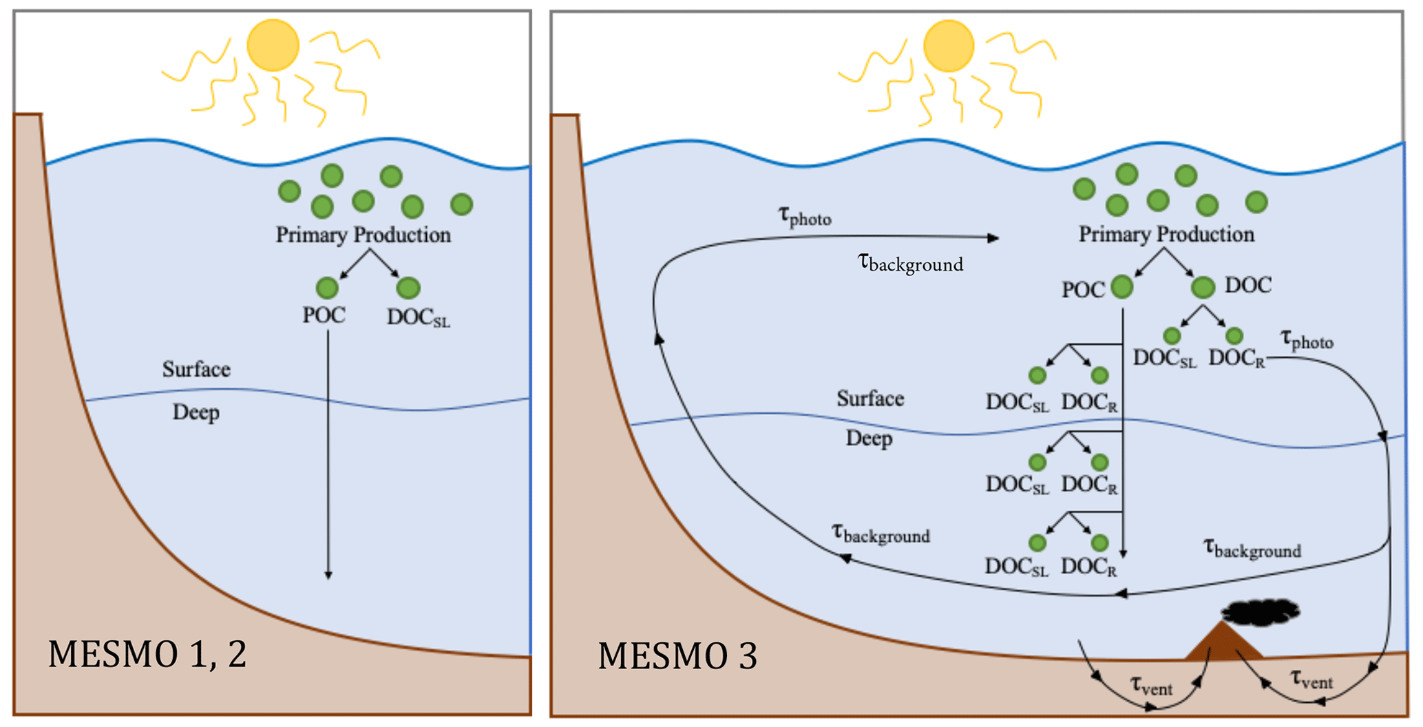
Figure 1 Schematic diagram of DOM cycling in MESMO 2 vs. MESMO 3. In the new model, DOM_r can be activated. DOM_r is produced from POM breakdown, which can occur in the production layer or throughout the water column in the “deep POC split”. Possible DOM_r remineralization mechanisms are the slow background degradation that occurs everywhere, thermal degradation in hydrothermal vents, and photodegradation at the surface. See the text for details.

The term fDOM denotes the fraction of NPP that is routed to DOM as opposed to POM. Likewise, fDOM_r is the fraction of DOM that is routed to DOM_r as opposed to DOM_sl. The value of fDOM_r is not well known but estimated to be ∼ 1 % (Hansell, 2013), which we tentatively adopt in MESMO 3. If DOM_r is not selected in the model run, fDOM_r=0. In previous versions of MESMO, fDOM was assigned a constant value of 0.67. In reality, a large variability is observed locally for this ratio, ranging from 0.01–0.2 in temperate waters to 0.1–0.7 in the Southern Ocean (Dunne et al., 2005; Henson et al., 2011; Laws et al., 2000). In MESMO 3, fDOM is calculated as a function of the ambient temperature following Laws et al. (2000):

$$\begin{array}{}\text{(19)}& \begin{array}{rl}& \mathrm{fDOM}=\\ & \mathrm{1.0}-min\left(\mathrm{0.72},max\left(\mathrm{0.04},\mathrm{0.62}-\mathrm{0.02}\cdot T\left({}^{\circ }\mathrm{C}\right)\right)\right).\end{array}\end{array}$$

This formulation gives low export efficiency (i.e., high fDOM) in the warmer regions compared to the colder high-latitude regions. Locally, we impose fixed fDOM upper and lower bounds of 0.96 and 0.28, respectively, as estimated from a previous study (Dunne et al., 2005).

In MESMO 3, a new DOM production pathway below the production layer is available as an option. In previous MESMO versions, sinking POM was respired in the water column with the loss of O₂ directly to the dissolved inorganic forms (i.e., POC → DIC, POP → PO₄, and PON → NO₃). In the new “deep POC split” pathway, sinking POM is simply broken down into DOM without the loss of O₂ as in the production layer (Fig. 1). If DOM_r is selected in the model, the broken-down POM is further routed to both DOM_sl and DOM_r according to fDOM_r. If not, all of the broken down POM is converted to DOM_sl. Thus, when the deep POC split is activated, the presence of DOM in the deep ocean can be accounted for by in situ production of DOM and DOM_r in addition to DOM transport from the surface. Thus, the deep POC split pathway offers an alternative means to control deep ocean DOM distribution.

2.4 Production of CaCO₃ and opal by eukaryotes

In MESMO 2, opal production was associated with the “large” PFT, and CaCO₃ production was associated with the “small” PFT. We recognize that coccolithophorids and diatoms, which are the producers of these biogenic tests, are both eukaryotes. Therefore, in MESMO 3, we associate both CaCO₃ and opal production with the POP production by the same eukaryote PFT (Jprod_POP1):

$$\begin{array}{}\text{(20)}& {\displaystyle }{\mathrm{Jprod}}_{{\mathrm{CaCO}}_{\mathrm{3}}}=r^{{\mathrm{CaCO}}_{\mathrm{3}}:\mathrm{POC}}\cdot {\mathrm{Jprod}}_{\mathrm{POP}\mathrm{1}}\cdot Q_{\mathrm{C},\mathrm{1}},\text{(21)}& {\displaystyle }{\mathrm{Jprod}}_{\mathrm{opal}}={\mathrm{Jprod}}_{\mathrm{POP}\mathrm{1}}\cdot Q_{\mathrm{Si}}.\end{array}$$

The concept of the residual nitrate potential growth (RNPG) (Balch et al., 2016) is useful in allowing competition between diatoms and non-siliceous phytoplankton within the same PFT (Matsumoto et al., 2020). Typically, in the real ocean, non-Si phytoplankton are able to grow faster and dominate the community if Si concentration is low and diatom growth is Si limited. Otherwise, diatoms are more competitive, as they have higher intrinsic growth rates. The RNPG index recasts the ambient concentrations of NO₃ and Si(OH)₄ into potential algal growth rates:

$$\begin{array}{}\text{(22)}& \mathrm{RNPG}={\displaystyle \frac{\left[{\mathrm{NO}}_{\mathrm{3}}\right]}{\left[{\mathrm{NO}}_{\mathrm{3}}\right]+K_{{\mathrm{NO}}_{\mathrm{3}},\mathrm{1}}}}-{\displaystyle \frac{\left[\mathrm{Si}{\left(\mathrm{OH}\right)}_{\mathrm{4}}\right]}{\left[\mathrm{Si}{\left(\mathrm{OH}\right)}_{\mathrm{4}}\right]+K_{\mathrm{Si}{\left(\mathrm{OH}\right)}_{\mathrm{4}}}}}.\end{array}$$

If RNPG is more positive, the index indicates that nitrate-dependent growth exceeds silica-dependent growth. Thus, non-Si phytoplankton are more competitive, and this leads to higher CaCO₃ production. On the other hand, a more negative RNPG implies that silica limitation for diatoms is relieved, leading to enhanced diatom growth and reduced CaCO₃ production. The RNPG index is incorporated in the calculation of the rain ratio $r^{{\mathrm{CaCO}}_{\mathrm{3}}:\mathrm{POC}}$ presented in Eq. (20) as follows:

$$\begin{array}{}\text{(23)}& \begin{array}{rl}& r^{{\mathrm{CaCO}}_{\mathrm{3}}:\mathrm{POC}}=r_{\mathrm{0}}^{{\mathrm{CaCO}}_{\mathrm{3}}:\mathrm{POC}}\cdot {\left(\mathrm{\Omega }-\mathrm{1}\right)}^{\mathit{\eta }}\\ & \cdot min\left(\mathrm{1},max\left(\mathrm{0.1},\mathrm{RNPG}\right)\right)\cdot k_{T,{\mathrm{CaCO}}_{\mathrm{3}}}.\end{array}\end{array}$$

Equation (23) indicates the base rain ratio $r_{\mathrm{0}}^{{\mathrm{CaCO}}_{\mathrm{3}}:\mathrm{POC}}$ (set to 0.30) is also modified by the carbonate ion saturation state Ω by η (set to 1.28) and temperature (see Ridgwell et al., 2007, and references therein):

$$\begin{array}{}\text{(24)}& {\displaystyle }\mathrm{\Omega }={\displaystyle \frac{\left[{\mathrm{Ca}}^{\mathrm{2}+}\right]\left[{\mathrm{CO}}_{\mathrm{3}}^{\mathrm{2}-}\right]}{K_{\mathrm{sp}}}},\text{(25)}& {\displaystyle }{k}_{T,{\mathrm{CaCO}}_{\mathrm{3}}}=min\left(\mathrm{1.0},{\displaystyle \frac{T\left({}^{\circ }\mathrm{C}\right)+\mathrm{2}}{T\left({}^{\circ }\mathrm{C}\right)+\mathrm{8}}}\right).\end{array}$$

K_sp is the solubility product of CaCO₃. The temperature dependency of CaCO₃ formation ($k_{T,{\mathrm{CaCO}}_{\mathrm{3}}}$) is similar to that of Moore et al. (2004) where warmer temperatures favor the growth of carbonate-bearing phytoplankton.

2.5 Remineralization of POM and DOM

Once produced, both POM and DOM undergo remineralization throughout the water column. Key remineralization parameter values are given in Table 2d. Previously, POM remineralization had a temperature dependence and decayed exponentially with depth (Yamanaka et al., 2004). In MESMO 3, we incorporate an additional dependency on dissolved oxygen following Laufkötter et al. (2017):

$$\begin{array}{}\text{(26)}& R_{{\mathrm{POM}}_i}=V_{\mathrm{POM}}\cdot e^{k_R\cdot T\cdot \frac{\left[{\mathrm{O}}_{\mathrm{2}}\right]}{\left[{\mathrm{O}}_{\mathrm{2}}\right]+K_{{\mathrm{O}}_{\mathrm{2}}}}}\cdot \left[{\mathrm{POM}}_i\right].\end{array}$$

V_POM is the base remineralization rate, k_R expresses the temperature sensitivity of remineralization, and $K_{{\mathrm{O}}_{\mathrm{2}}}$ is half-saturation constant for oxygen-dependent remineralization. When the sediment model is not coupled, any POM that reaches the seafloor dissolves completely to its inorganic form and is returned to the overlying water.

In MESMO 3, all forms of semi-labile DOM remineralize at the same rate. It is represented by τ_sl, the inverse of the timescale of DOM_sl decay, which has been estimated previously to be ∼ 1.5 years (Hansell, 2013):

$$\begin{array}{}\text{(27)}& R_{{\mathrm{DOM}}_{\mathrm{sl}}}={\mathit{\tau }}_{\mathrm{sl}}\cdot \left[{\mathrm{DOM}}_{\mathrm{sl}}\right].\end{array}$$

All forms of DOM_r also remineralize at the same rate in MESMO 3. In total, there are three optional, additive sinks of DOM_r in the model: slow background decay, photodegradation, and degradation via hydrothermal vents (Fig. 1). Observations clearly indicate that the ¹⁴C age of deep-ocean DOC_r is 10³ years (e.g., Druffel et al., 1992), much older than DI¹⁴C. In addition, the deep ocean DOC_r concentration decreases modestly along the path of the deep water from the deep North Atlantic to the deep North Pacific (Hansell and Carlson, 1998). Thus, it is understood that there is a slow DOM_r background decay in the deep ocean. We represent this ubiquitous process with τ_bg, which is the inverse of the background decay timescale, estimated to be ∼ 16 000 years (Hansell, 2013).

Observations to date indicate that photodegradation is a major sink of DOM_r (e.g., Mopper et al., 1991). This process is believed to convert DOM_r that is upwelled from the ocean interior into the euphotic zone into more labile forms of DOM. We represent photodegradation with τ_photo, the inverse of the decay timescale, estimated to be ∼ 70 years (Yamanaka and Tajika, 1997). This occurs only in the surface.

Finally, observations of DOM emanating from different types of hydrothermal vents indicate that they have variable impacts on the deep-sea DOM_r (Lang et al., 2006). However, the off-axis vents circulate far more seawater through the fractured oceanic crust than the high-temperature and diffuse vents and are thus believed to determine the overall impact of the vents on the deep-sea DOM_r as a net sink (Lang et al., 2006). Here we assume simply that seawater that circulates through the vents loses all DOM_r (i.e., $\mathrm{1}/{\mathit{\tau }}_{\mathrm{vent}}$ < Δt, where Δt is the biogeochemical model time step of 0.05 year). This means that the more seawater circulates through the vents, the more DOM_r is removed: the total removal rate depends on the vent flux of seawater H_flux. We implement the vent degradation of DOM_r in MESMO 3 by first identifying the wet grid boxes located immediately above known mid-ocean ridges. We then distribute the annual global H_flux of 4.8×10¹⁶ kg yr⁻¹ (Lang et al., 2006) equally among those ridge-associated grid boxes. The grid cells contain a mass of seawater much greater than the mass that circulates through vents in Δt (10²¹ kg vs. 10¹³ kg). Therefore, the seawater mass in the vent grid cells that does not circulate through the vents in Δt is subject only to background degradation in MESMO 3.

The three DOM_r sinks are not mutually exclusive. They can thus be combined to yield the total DOM_r remineralization rate:

$$\begin{array}{}\text{(28)}& R_{{\mathrm{DOM}}_{\mathrm{r}}}=\left({\mathit{\tau }}_{\mathrm{bg}}+{\mathit{\tau }}_{\mathrm{photo}}+{\mathit{\tau }}_{\mathrm{vent}}\cdot {\displaystyle \frac{{\mathrm{SW}}_{\text{flux\_local}}}{{\mathrm{SW}}_{\mathrm{grid}}}}\right)\cdot \left[{\mathrm{DOM}}_{\mathrm{r}}\right],\end{array}$$

where SW_{flux_local} is the mass of seawater that circulates through the vents in each grid box in Δt, and SW_grid is the total mass of seawater in the same grid box.

The amount of O₂ respired as a result of these POM and DOM remineralization processes is related to the organic carbon pools by the respiratory quotients of POC and DOC, $r_{-{\mathrm{O}}_{\mathrm{2}}:\mathrm{POC}}$ and $r_{-{\mathrm{O}}_{\mathrm{2}}:\mathrm{DOC}}$, respectively. These are molar ratios of O₂ consumed per unit organic carbon respired. They are variable and calculated from the ambient POM and DOM concentration (Tanioka and Matsumoto, 2020b):

$$\begin{array}{}\text{(29)}& {\displaystyle }{r}_{-{\mathrm{O}}_{\mathrm{2}}:\mathrm{POC}}=\mathrm{1.1}+{\displaystyle \frac{\mathrm{2}\left[\mathrm{PON}\right]}{\left[\mathrm{POC}\right]}},\text{(30)}& {\displaystyle }{r}_{-{\mathrm{O}}_{\mathrm{2}}:\mathrm{DOC}}=\mathrm{1.1}+{\displaystyle \frac{\mathrm{2}\left[\mathrm{DON}\right]}{\left[\mathrm{DOC}\right]}}.\end{array}$$

2.6 Remineralization of CaCO₃ and opal

Remineralization of CaCO₃ and opal particles occurs as they sink through the water column and remains the same as in MESMO 2. Key parameter values are given in Table 2d. Remineralization of CaCO₃ is a function of temperature similar to that of particulate organic matter remineralization but without oxygen dependency. The temperature-dependence term k_R modifies the base remineralization rate $V_{{\mathrm{CaCO}}_{\mathrm{3}}}$:

$$\begin{array}{}\text{(31)}& R_{{\mathrm{CaCO}}_{\mathrm{3}}}=V_{{\mathrm{CaCO}}_{\mathrm{3}}}\cdot e^{k_R\cdot T}\cdot \left[{\mathrm{CaCO}}_{\mathrm{3}}\right].\end{array}$$

Opal remineralization in the water column follows Ridgwell et al. (2002). The rate of opal remineralization R_opal is given by the product of normalized dissolution rate (r_opal), base opal dissolution rate (k_opal), and opal concentration [opal].

$$\begin{array}{}\text{(32)}& {\displaystyle }{R}_{\mathrm{opal}}=r_{\mathrm{opal}}\cdot k_{\mathrm{opal}}\cdot \left[\mathrm{opal}\right]\text{(33)}& {\displaystyle }\begin{array}{rl}& r_{\mathrm{opal}}=\mathrm{0.16}\cdot \left(\mathrm{1}+{\displaystyle \frac{T\left({}^{\circ }\mathrm{C}\right)}{\mathrm{15}}}\right)\cdot u_{\mathrm{opal}}+\mathrm{0.55}\\ & \cdot {\left({\left(\mathrm{1}+{\displaystyle \frac{T\left({}^{\circ }\mathrm{C}\right)}{\mathrm{400}}}\right)}^{\mathrm{4}}\cdot u_{\mathrm{opal}}\right)}^{\mathrm{9.25}}\end{array}\text{(34)}& {\displaystyle }{u}_{\mathrm{opal}}={\displaystyle \frac{{\left[\mathrm{Si}{\left(\mathrm{OH}\right)}_{\mathrm{4}}\right]}_{\mathrm{eq}}-\left[\mathrm{Si}{\left(\mathrm{OH}\right)}_{\mathrm{4}}\right]}{{\left[\mathrm{Si}{\left(\mathrm{OH}\right)}_{\mathrm{4}}\right]}_{\mathrm{eq}}}}\end{array}$$

r_opal is a function of temperature (T) and the degree of under-saturation (u_opal), which in turn is calculated from the ambient [Si(OH)₄] and [Si(OH)₄] at equilibrium. The equilibrium concentration is a function of ambient temperature:

$$\begin{array}{}\text{(35)}& {\log }_{\mathrm{10}}\left({\left[\mathrm{Si}{\left(\mathrm{OH}\right)}_{\mathrm{4}}\right]}_{\mathrm{eq}}\right)=\mathrm{6.44}-{\displaystyle \frac{\mathrm{968}}{T\left(\mathrm{K}\right)}}.\end{array}$$

Without the sediment module of MESMO activated, both CaCO₃ and opal particles that reach the seafloor are completely dissolved back to inorganic forms.

2.7 Conservation of organic matter and biogenic tests

The time rate of change of the biogenic organic matter and tests are given by the sum of the production terms (i.e., sources) and the remineralization terms (i.e., sinks). The circulation-related transport terms are omitted as noted above, but the vertical transport due to particle sinking is included here. The sinking speed w is the same for all particles. The sum of POM_i of all the PFTs give the total POM concentrations.

$$\begin{array}{}\text{(36)}& {\displaystyle \frac{\partial {\left[\mathrm{POP}\right]}_i}{\partial t}}={\mathrm{Jprod}}_{{\mathrm{POP}}_i}-{\displaystyle \frac{\partial }{\partial z}}\left(w{\left[\mathrm{POP}\right]}_i\right)-R_{\mathrm{POP},i}\text{(37)}& {\displaystyle \frac{\partial {\left[\mathrm{POC}\right]}_i}{\partial t}}={\mathrm{Jprod}}_{{\mathrm{POP}}_i}\cdot Q_{\mathrm{C},i}-{\displaystyle \frac{\partial }{\partial z}}\left(w{\left[\mathrm{POC}\right]}_i\right)-R_{\mathrm{POC},i}\text{(38)}& {\displaystyle \frac{\partial {\left[\mathrm{PON}\right]}_i}{\partial t}}={\mathrm{Jprod}}_{{\mathrm{POP}}_i}\cdot Q_{\mathrm{N},i}-{\displaystyle \frac{\partial }{\partial z}}\left(w{\left[\mathrm{PON}\right]}_i\right)-R_{\mathrm{PON},i}\text{(39)}& {\displaystyle \frac{\partial {\left[\mathrm{POFe}\right]}_i}{\partial t}}={\mathrm{Jprod}}_{{\mathrm{POP}}_i}\cdot Q_{\mathrm{Fe},i}-{\displaystyle \frac{\partial }{\partial z}}\left(w{\left[\mathrm{POFe}\right]}_i\right)-R_{\mathrm{POFe},i}\text{(40)}& {\displaystyle }\left[\mathrm{POM}\right]={\sum }_i{\left[\mathrm{POM}\right]}_i\end{array}$$

The time rate of change of CaCO₃ and opal is expressed in much the same way as POM.

$$\begin{array}{}\text{(41)}& {\displaystyle \frac{\partial \left[{\mathrm{CaCO}}_{\mathrm{3}}\right]}{\partial t}}={\mathrm{Jprod}}_{{\mathrm{CaCO}}_{\mathrm{3}}}-{\displaystyle \frac{\partial }{\partial z}}\left(w\left[{\mathrm{CaCO}}_{\mathrm{3}}\right]\right)-R_{{\mathrm{CaCO}}_{\mathrm{3}}}\text{(42)}& {\displaystyle \frac{\partial \left[\mathrm{opal}\right]}{\partial t}}={\mathrm{Jprod}}_{\mathrm{opal}}-{\displaystyle \frac{\partial }{\partial z}}\left(w\left[\mathrm{opal}\right]\right)-R_{\mathrm{opal}}\end{array}$$

The DOM pools have the production and remineralization terms without the particle sinking term.

$$\begin{array}{}\text{(43)}& {\displaystyle \frac{\partial \left[{\mathrm{DOP}}_{\mathrm{sl}}\right]}{\partial t}}={\mathrm{Jprod}}_{{\mathrm{DOP}}_{\mathrm{sl}}}-R_{{\mathrm{DOP}}_{\mathrm{sl}}}\text{(44)}& {\displaystyle \frac{\partial \left[{\mathrm{DON}}_{\mathrm{sl}}\right]}{\partial t}}={\mathrm{Jprod}}_{{\mathrm{DON}}_{\mathrm{sl}}}-R_{{\mathrm{DON}}_{\mathrm{sl}}}\text{(45)}& {\displaystyle \frac{\partial \left[{\mathrm{DOC}}_{\mathrm{sl}}\right]}{\partial t}}={\mathrm{Jprod}}_{{\mathrm{DOC}}_{\mathrm{sl}}}-R_{{\mathrm{DOC}}_{\mathrm{sl}}}\text{(46)}& {\displaystyle \frac{\partial \left[{\mathrm{DOFe}}_{\mathrm{sl}}\right]}{\partial t}}={\mathrm{Jprod}}_{{\mathrm{DOFe}}_{\mathrm{sl}}}-R_{{\mathrm{DOFe}}_{\mathrm{sl}}}\text{(47)}& {\displaystyle \frac{\partial \left[{\mathrm{DOP}}_{\mathrm{r}}\right]}{\partial t}}={\mathrm{Jprod}}_{{\mathrm{DOP}}_{\mathrm{r}}}-R_{{\mathrm{DOP}}_{\mathrm{r}}}\text{(48)}& {\displaystyle \frac{\partial \left[{\mathrm{DON}}_{\mathrm{r}}\right]}{\partial t}}={\mathrm{Jprod}}_{{\mathrm{DON}}_{\mathrm{r}}}-R_{{\mathrm{DON}}_{\mathrm{r}}}\text{(49)}& {\displaystyle \frac{\partial \left[{\mathrm{DOC}}_{\mathrm{r}}\right]}{\partial t}}={\mathrm{Jprod}}_{{\mathrm{DOC}}_{\mathrm{r}}}-R_{{\mathrm{DOC}}_{\mathrm{r}}}\end{array}$$

2.8 Conservation of inorganic nutrients

The time rate of change of the inorganic nutrients have organic carbon production as sink terms and remineralization as source terms. The production terms (J_prod) are zero below the upper-ocean production layer. Nutrients have a unit of mol element kg⁻¹ in the model.

$$\begin{array}{}\text{(50)}& {\displaystyle \frac{\partial \left[{\mathrm{PO}}_{\mathrm{4}}\right]}{\partial t}}=-\sum _i{\mathrm{\Gamma }}_i+\sum _i{R}_{\mathrm{POP},i}+R_{{\mathrm{DOP}}_{\mathrm{sl}}}+R_{{\mathrm{DOP}}_{\mathrm{r}}}\text{(51)}& {\displaystyle }\begin{array}{rl}& {\displaystyle \frac{\partial \left[{\mathrm{NO}}_{\mathrm{3}}\right]}{\partial t}}=-\sum _i{\mathrm{\Gamma }}_i\cdot Q_{\mathrm{N},i}+\sum _i{R}_{\mathrm{PON},i}\\ & +R_{{\mathrm{DON}}_{\mathrm{sl}}}+R_{{\mathrm{DON}}_{\mathrm{r}}}+{\mathrm{Fix}}_{\mathrm{N}}-{\mathrm{Den}}_{\mathrm{N}}\end{array}\text{(52)}& {\displaystyle }\begin{array}{rl}& {\displaystyle \frac{\partial \left[\mathrm{DIC}\right]}{\partial t}}=-\left(\sum _i{\mathrm{\Gamma }}_i{Q}_{\mathrm{C},i}+{\mathrm{Jprod}}_{{\mathrm{CaCO}}_{\mathrm{3}}}\right)+\sum _i{R}_{\mathrm{POC},i}\\ & +R_{{\mathrm{DOC}}_{\mathrm{sl}}}+R_{{\mathrm{DOC}}_{\mathrm{r}}}+R_{{\mathrm{CaCO}}_{\mathrm{3}}}+F_{\mathrm{gas},{\mathrm{CO}}_{\mathrm{2}}}\end{array}\text{(53)}& {\displaystyle }\begin{array}{rl}& {\displaystyle \frac{\partial \left[\mathrm{ALK}\right]}{\partial t}}=-\left(\mathrm{2}\cdot {\mathrm{Jprod}}_{{\mathrm{CaCO}}_{\mathrm{3}}}-\sum _i{\mathrm{\Gamma }}_i{Q}_{\mathrm{N},i}\right)-\sum _i{R}_{\mathrm{PON},i}\\ & -R_{{\mathrm{DON}}_{\mathrm{sl}}}-R_{{\mathrm{DON}}_{\mathrm{r}}}-{\mathrm{Fix}}_{\mathrm{N}}+{\mathrm{Den}}_{\mathrm{N}}+\mathrm{2}\cdot R_{{\mathrm{CaCO}}_{\mathrm{3}}}\end{array}\text{(54)}& {\displaystyle }\begin{array}{rl}& {\displaystyle \frac{\partial \left[\mathrm{FeT}\right]}{\partial t}}=-\sum _i{\mathrm{\Gamma }}_i{Q}_{\mathrm{Fe},i}+\sum _i{R}_{\mathrm{POFe},i}\\ & +R_{{\mathrm{DOFe}}_{\mathrm{sl}}}+R_{{\mathrm{POM}}_{\mathrm{Fe}}}+{\mathrm{Aeolian}}_{\mathrm{Fe}}\end{array}\text{(55)}& {\displaystyle \frac{\partial \left[\mathrm{Si}{\left(\mathrm{OH}\right)}_{\mathrm{4}}\right]}{\partial t}}=-{\mathrm{Jprod}}_{\mathrm{opal}}+R_{\mathrm{opal}}\text{(56)}& {\displaystyle }\begin{array}{rl}& {\displaystyle \frac{\partial \left[{\mathrm{O}}_{\mathrm{2}}\right]}{\partial t}}=\sum _i{\mathrm{\Gamma }}_i\cdot Q_{{-\mathrm{O}}_{\mathrm{2}},i}-(r_{-{\mathrm{O}}_{\mathrm{2}}:\mathrm{DOC}}\\ & \cdot \left(R_{{\mathrm{DOC}}_{\mathrm{sl}}}+R_{{\mathrm{DOC}}_{\mathrm{r}}}\right)+\sum _i{r}_{-{\mathrm{O}}_{\mathrm{2}}:\mathrm{POC},i}\cdot R_{\mathrm{POC},i})\\ & +\mathrm{1.25}{\mathrm{Den}}_{\mathrm{N}}+F_{\mathrm{gas},{\mathrm{O}}_{\mathrm{2}}}\end{array}\end{array}$$

In Eq. (51), Fix_N is the N fixation carried out by diazotrophs, and Den_N is the water column denitrification. There is an air–sea gas exchange term F_gas in Eqs. (52) and (56) for gaseous CO₂ and O₂, respectively. In Eq. (53), alkalinity increases with decreasing nitrate concentrations and increasing CaCO₃ dissolution. Equation (54) contains R_POMFe, which is an iron source that represents remineralization of the Fe^′ scavenged by sinking particles. These terms are explained in the following sections.

2.9 Prognostic nitrogen cycle

Biological production by diazotrophs is stimulated when the ambient NO₃ is low. Nitrogen fixed by diazotrophs during their growth is added to the marine NO₃ pool. The prognostic nitrogen fixation model employed here is similar to that used in the HAMOCC biogeochemical module (Paulsen et al., 2017):

$$\begin{array}{}\text{(57)}& {\displaystyle }{\mathrm{Fix}}_{\mathrm{N}}={\mathrm{\Gamma }}_{\mathrm{3}}\cdot Q_{\mathrm{N},\mathrm{3}}\cdot I_{{\mathrm{NO}}_{\mathrm{3}}},\text{(58)}& {\displaystyle }{I}_{{\mathrm{NO}}_{\mathrm{3}}}=\left(\mathrm{1.0}-{\displaystyle \frac{{\left[{\mathrm{NO}}_{\mathrm{3}}\right]}^{\mathrm{2}}}{K_{{\mathrm{NO}}_{\mathrm{3}}\mathrm{\_}\mathrm{Nfix}}^{\mathrm{2}}+{\left[{\mathrm{NO}}_{\mathrm{3}}\right]}^{\mathrm{2}}}}\right),\end{array}$$

where Fix_N is the nitrogen fixation rate and $I_{{\mathrm{NO}}_{\mathrm{3}}}$ is the nitrate dependency term in quadratic Michaelis–Menten kinetics form with the half-saturation constant $K_{{\mathrm{NO}}_{\mathrm{3}}\mathrm{\_}\mathrm{Nfix}}$. See Table 2e for the values related to the N cycle.

Water column denitrification is formulated in an approach similar to that of the original GENIE model (Ridgwell et al., 2007), in which 2 mol of NO₃ are converted to 1 mol of N₂ and liberating 2.5 mol of O₂ as a byproduct:

$$\begin{array}{}\text{(59)}& \mathrm{2}{\mathrm{NO}}_{\mathrm{3}}^{-}+\mathrm{2}{\mathrm{H}}^{+}\to \mathrm{2.5}{\mathrm{O}}_{\mathrm{2}}+{\mathrm{N}}_{\mathrm{2}}+{\mathrm{H}}_{\mathrm{2}}\mathrm{O}.\end{array}$$

Denitrification takes place in grid boxes, in which O₂ concentration is below a threshold concentration (O_2,def) and is stimulated if the total global inventory of NO₃ relative to PO₄ is high. In other words, denitrification can effectively act as negative feedback to nitrogen fixation. The threshold O₂ concentration (O_2,def) takes the minimum of the hard-bound O₂ threshold concentration (O_2,crit) and the NO₃ to PO₄ ratio, scaled by a parameter k_D. The parameters O_2,crit and k_D are calibrated to give the global denitrification rate of roughly 100 Tg N yr⁻¹, which balances the total nitrogen fixation rate in the model.

$$\begin{array}{}\text{(60)}& {\displaystyle }{\mathrm{Den}}_{\mathrm{N}}=\mathrm{0.8}\left[{\mathrm{yr}}^{-\mathrm{1}}\right]\cdot max\left(\left({\left[{\mathrm{O}}_{\mathrm{2}}\right]}_{\mathrm{def}}-\left[{\mathrm{O}}_{\mathrm{2}}\right]\right),\mathrm{0}\right)\text{(61)}& {\displaystyle }{\left[{\mathrm{O}}_{\mathrm{2}}\right]}_{\mathrm{def}}=min\left({\mathrm{O}}_{\mathrm{2},\mathrm{crit}},k_D\cdot {\displaystyle \frac{{\left[{\mathrm{NO}}_{\mathrm{3}}\right]}_{\mathrm{inventory}}}{{\left[{\mathrm{PO}}_{\mathrm{4}}\right]}_{\mathrm{inventory}}}}\right)\end{array}$$

2.10 Prognostic iron cycle

The iron cycle in MESMO 3 remains the same as in MESMO 2. Key parameter values are given in Table 2e. The two species of dissolved iron (Fe^′ and FeL) are partitioned according to the following equilibrium relationship:

$$\begin{array}{}\text{(62)}& K_{\mathrm{ligand}}={\displaystyle \frac{\left[\mathrm{FeL}\right]}{\left[{\mathrm{Fe}}^{\prime }\right]\cdot \left[L\right]}},\end{array}$$

where [L] is the ligand concentration and K_ligand is the conditional stability constant. The sum of ligand and FeL is set at a constant value of 1 nmol kg⁻¹ everywhere. Iron is introduced into the model domain by a constant fraction (3.5 wt %) of aeolian dust deposition at the surface (F_in) following the prescribed modern flux pattern (Mahowald et al., 2006) with constant solubility (β):

$$\begin{array}{}\text{(63)}& S_{\mathrm{Fe}}=\mathit{\beta }\cdot F_{\mathrm{in}}.\end{array}$$

Particle-scavenged iron POM_Fe (note the difference from POFe) is produced below the productive layer when sinking POM scavenges Fe^′ to sinking POM:

$$\begin{array}{}\text{(64)}& J_{\mathrm{Fe}}=-{\mathit{\tau }}_{\mathrm{sc}}\cdot K_o\cdot {\left[\mathrm{POC}\right]}^{\mathrm{0.58}}\cdot \left[{\mathrm{Fe}}^{\prime }\right],\end{array}$$

where τ_sc and K_o are empirical parameters that determine the strength of scavenging. Remineralization of Fe scavenged to POM (POM_Fe) is identical in form to that of POM remineralization:

$$\begin{array}{}\text{(65)}& R_{{\mathrm{POM}}_{\mathrm{Fe}}}=V_{\mathrm{POM}}\cdot e^{k_{R}T\cdot \frac{\left[{\mathrm{O}}_{\mathrm{2}}\right]}{\left[{\mathrm{O}}_{\mathrm{2}}\right]+K_{{\mathrm{O}}_{\mathrm{2}}}}}\cdot \left[{\mathrm{POM}}_{\mathrm{Fe}}\right].\end{array}$$

The conservation equation of the particle scavenged iron is thus expressed as follows:

$$\begin{array}{}\text{(66)}& {\displaystyle \frac{\partial \left[{\mathrm{POM}}_{\mathrm{Fe}}\right]}{\partial t}}=J_{\mathrm{Fe}}-{\displaystyle \frac{\partial }{\partial z}}\left(w\left[{\mathrm{POM}}_{\mathrm{Fe}}\right]\right)-R_{{\mathrm{POM}}_{\mathrm{Fe}}}.\end{array}$$

Any scavenged iron that escapes remineralization in the water column reaching the seafloor is removed from the model domain in order to keep the total Fe inventory at a steady state.

2.11 Air–sea gas exchange

The air–sea gas exchange formulation remains the same as in MESMO 2 and follows Ridgwell et al. (2007). It is the function of gas transfer velocity, the ambient dissolved gas concentration, and saturation gas concentration. The flux of CO₂ and O₂ gases across the air–sea interface is given by

$$\begin{array}{}\text{(67)}& {\displaystyle }{F}_{\mathrm{gas},{\mathrm{CO}}_{\mathrm{2}}}=k\cdot \left({\left[{\mathrm{CO}}_{\mathrm{2}}\right]}_{\mathrm{sat}}-\left[{\mathrm{CO}}_{\mathrm{2}}\right]\right)\cdot \left(\mathrm{1}-A\right),\text{(68)}& {\displaystyle }{F}_{\mathrm{gas},{\mathrm{O}}_{\mathrm{2}}}=k\cdot \left({\left[{\mathrm{O}}_{\mathrm{2}}\right]}_{\mathrm{sat}}-\left[{\mathrm{O}}_{\mathrm{2}}\right]\right)\cdot \left(\mathrm{1}-A\right),\end{array}$$

where k is the gas transfer velocity, ${\left[{\mathrm{CO}}_{\mathrm{2}}\right]}_{\mathrm{sat}}$ and ${\left[{\mathrm{O}}_{\mathrm{2}}\right]}_{\mathrm{sat}}$ are saturation concentrations, and A is the fractional ice-covered area that is calculated by the physical model. Gas transfer velocity k is a function of wind speed (u) following Wanninkhof (1992) where Sc is the Schmidt number for a specific gas:

$$\begin{array}{}\text{(69)}& k=\mathrm{0.31}\cdot u^{\mathrm{2}}\cdot {\left({\displaystyle \frac{Sc}{\mathrm{660}}}\right)}^{-\mathrm{0.5}}.\end{array}$$

3 Results and discussion

All new results from MESMO 3 presented here are from the steady state. On a single computer core at the Minnesota Supercomputing Institute, it takes approximately 1 h to complete 1000 years of MESMO 3 simulation. The “standard” MESMO 3 has the power law model of flexible stoichiometry but no DOM_r. The results from the standard model (hereafter just MESMO 3) are presented in Sect. 3.1, and the results from the DOM_r-enabled model are presented in Sect. 3.2. In Table 3, we summarize and compare key biogeochemical diagnostics from MESMO 3 against those from MESMO 2 and available observational constraints. The global NPP, as well as global export production of POC and opal, are comparable or somewhat lower in MESMO 3 than MESMO 2.

Table 3 Key Biogeochemical diagnostics

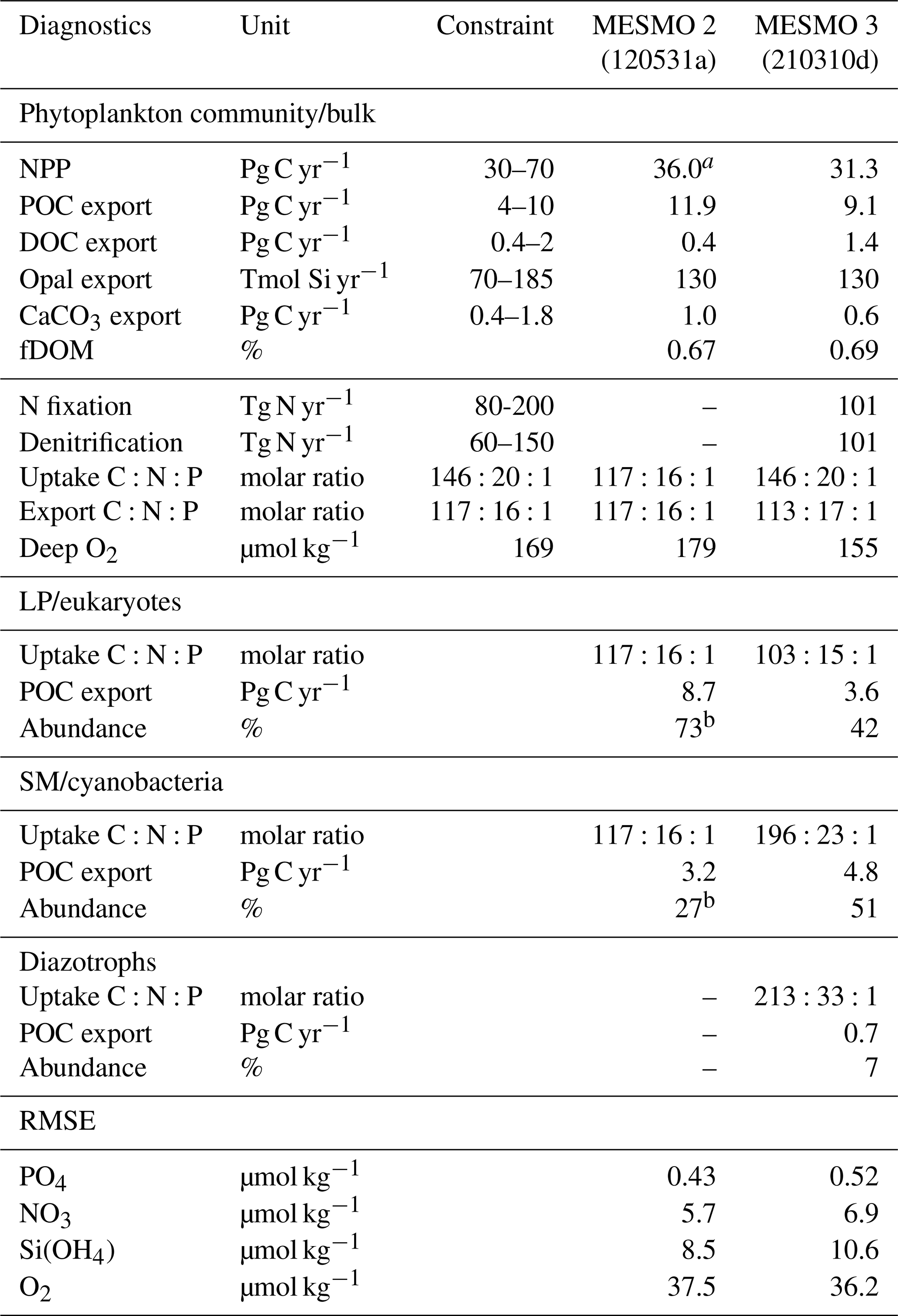
^a NPP for MESMO 2 was unavailable as a model output and is therefore estimated from POC and fDOM = 0.67. ^b NPP (in terms of C) is needed in the calculation of the PFT abundance. The root-mean-square error (RMSE) of the simulated P, N, Si, and O₂ distributions from MESMO 2 and 3 was calculated relative to the World Ocean Atlas 2018 (WOA18) gridded data (Garcia et al., 2018, 2019). The model–data comparison is made in the top 100 m for nutrients and below 100 m for O₂. WOA18 was regridded to the MESMO 3 grid to calculate the RMSE. References for independent constraints are as follows: (1) global NPP (Carr et al., 2006), (2) global POC export (DeVries and Weber, 2017), (3) global DOC export assumed to be 20 % of total carbon export (Hansell et al., 2009; Roshan and DeVries, 2017), (4) global opal (Dunne et al., 2007), (5) global CaCO₃ export (Berelson et al., 2007), (6) global N fixation and denitrification rates (Landolfi et al., 2018), (7) uptake $\mathrm{C}:\mathrm{N}:\mathrm{P}$ ratio is based on POM measurements (Martiny et al., 2013), (8) export $\mathrm{C}:\mathrm{N}:\mathrm{P}$ ratio is assumed to equal the subsurface remineralization ratio (Anderson and Sarmiento, 1994), and (9) deep O₂ from WOA18 below 100 m (Garcia et al., 2019).

We relied on experience to calibrate MESMO 3 with the primary goal of reasonably simulating the phytoplankton community composition and $\mathrm{C}:\mathrm{N}:\mathrm{P}$ ratio (e.g., abundant cyanobacteria and high ratio for all PFTs in oligotrophic gyres). We tried to improve or at least preserve the gains that we achieved in earlier versions of MESMO in terms of the global distributions of PO₄, NO₃, O₂, Si(OH)₄, and FeT (Supplement Figs. S1, S2, S3, S4, and S5). Overall, there is a stronger nutrient depletion in the new model. For example, the surface PO₄ and NO₃ in MESMO 3 are now sufficiently depleted in the subtropical gyres but are too low in the eastern equatorial Pacific when compared to the World Ocean Atlas (Fig. S1; see RMSE in Table 3). It is a challenge for MESMO and other coarse-resolution models to simulate narrow dynamical features such as equatorial upwelling and reproduce biogeochemical features with sharp gradients. The spatial pattern of POC export that drives this surface nutrient pattern is similar in the two models (Fig. S2). In the 1D global profile, there is a marked improvement in the subsurface distribution of O₂ in MESMO 3 over MESMO 2. Whereas the depth of the oxygen minimum was ∼ 300 m in MESMO 2, it is ∼ 1000 m in both MESMO 3 and the World Ocean Atlas (Fig. S3). At 1000 m, the O₂ minimum is located in the far North Pacific in MESMO 3, whereas in the World Ocean Atlas it occurs in both the Northeast Pacific and the Arabian Sea. In contrast, the world ocean at 1000 m is too well oxygenated in MESMO 2. We believe that the improved match in the O₂ minimum depth would help simulate denitrification in the correct depth range, and there is a modest improvement in the data–model O₂ mismatch in terms of RMSE in MESMO 3 over MESMO 2 (Table 3). The deepening of the O₂ minimum was achieved largely by increasing the particle sinking speed, which tends to strengthen the biological pump and deplete the surface nutrients. This also helps MESMO 3 preserve MESMO 2's surface Si(OH)₄ depletion in much of the world ocean except in the North Pacific and Southern Ocean (Fig. S4). This is a feature captured by Si^* < 0 (Si${}^{*}=$[Si(OH)₄]-[NO₃]) in observations (Sarmiento et al., 2004) and simulated previously by MESMO 2 and now MESMO 3. Finally, surface FeT is also depleted more strongly in MESMO 3 over MESMO 2, except the North Atlantic, where aeolian deposition of dust from the Sahara maintains a steady Fe supply (Fig. S5).

In MESMO 3, we made no effort to calibrate all the semi-labile pools of DOM: DOC_sl, DOP_sl, DON_sl, and DOFe_sl. We note only that the surface DOC_sl concentration of 58 µmol kg⁻¹ and DOC export production of 1.4 Pg C yr⁻¹ in MESMO 3 are higher than in MESMO 2 (24 µmol kg⁻¹ and 0.4 Pg C yr⁻¹, respectively). The higher surface concentration is due to the longer τ_sl in MESMO 3 (Table 2d). The global average of the temperature-dependent fDOM in MESMO 3 is 0.69, which is slightly higher than the spatially uniform value of 0.67 in MESMO 2.

3.1 Novel features of MESMO 3

An important new feature of MESMO 3 is the representation of the primary producers by three PFTs (Fig. 2). The eukaryotes are characterized by the highest maximum growth rate and high half-saturation constants. Thus, the eukaryotes are more dominant than the other PFTs in the more eutrophic waters of the equatorial and polar regions (Fig. 2a). The cyanobacteria have smaller half-saturation constants and thus are more dominant in the oligotrophic subtropical gyres (Fig. 2c). The diazotrophs do not have NO₃ limitation but have the lowest maximum growth rate. Thus it is much lower in abundance than the other two PFTs generally, and out-competed in transient blooms and thus excluded in higher latitudes (Fig. 2e).

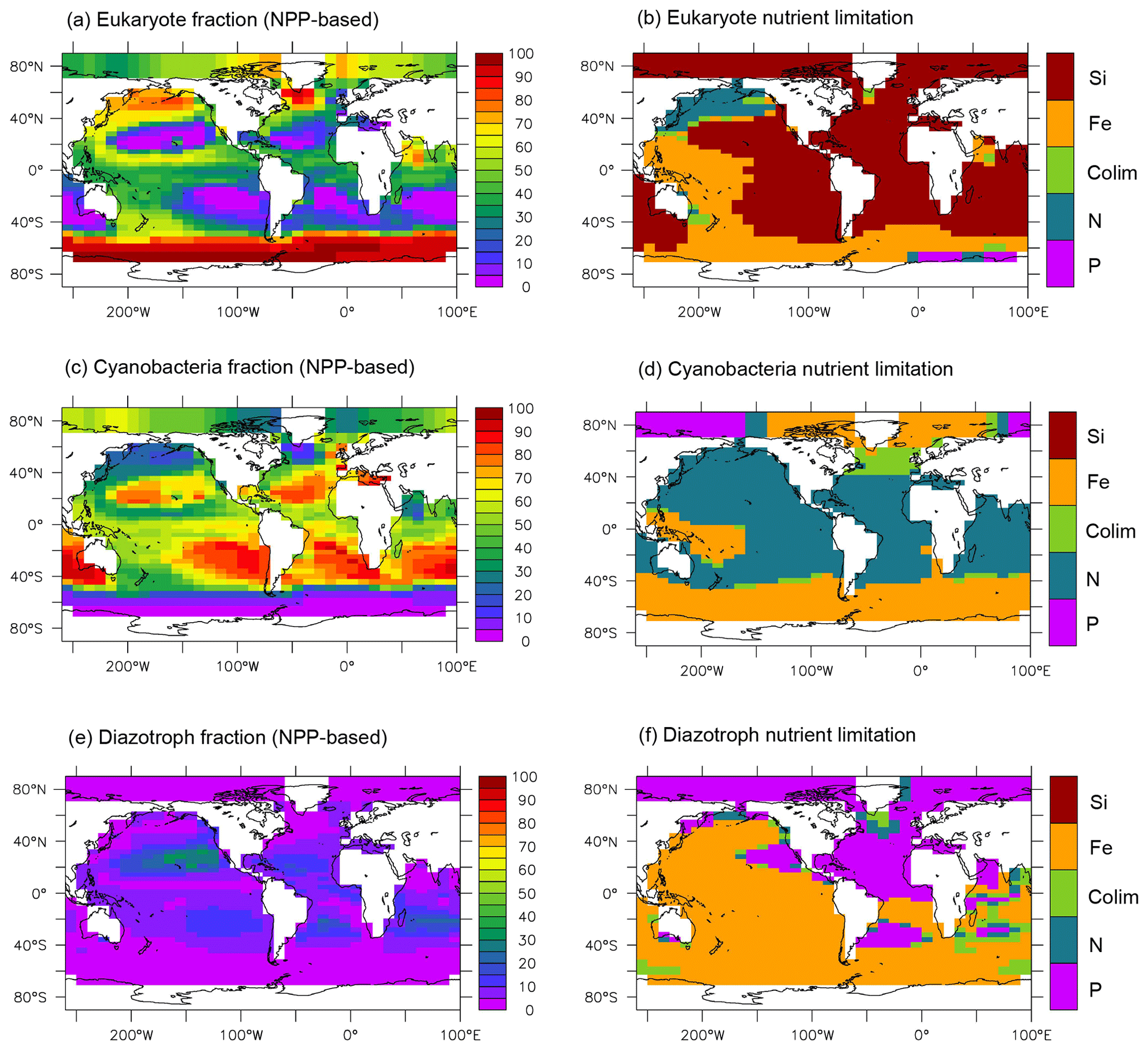
Figure 2 NPP-based surface phytoplankton functional type (PFT) abundance and nutrient limitation in MESMO 3. Fractional abundance and nutrient limitation for eukaryotes (a, b), cyanobacteria (c, d), and diazotrophs (e, f).

Figure 2 also indicates that all three PFTs show Fe limitation in the Southern Ocean. Outside the Southern Ocean, the eukaryotes are primarily limited by Si(OH)₄ (Fig. 2b). As far as organic carbon is concerned, we consider the eukaryotes to basically represent diatoms, which are arguably the most important agent of organic carbon export. In this context, the widespread silica limitation for eukaryotes would be consistent with the notions that silica uptake by diatoms should be limited in ∼ 60 % of the world surface ocean (Ragueneau et al., 2000) and that much the world ocean thermocline is filled with silica-depleted water (Si^* < 0 as noted above). On the other hand, the cyanobacteria are largely limited by NO₃ outside the Southern Ocean (Fig. 2d). The diazotrophs are limited by iron in much of the world ocean except in the Atlantic basin (Fig. 2f), where surface PO₄ is strongly depleted in both observations (Mather et al., 2008) and in our model (Fig. S1).

Figure 3 illustrates the influence of the RNPG index, which was implemented in MESMO 3 to allow for the effect of competition between diatoms and coccolithophores within the same PFT (Eqs. 22 and 23). The eukaryote NPP (Fig. 3a) is effectively split into two parts: one is associated with diatoms and opal production (Fig. 3b), and the other is associated with coccolithophores and CaCO₃ production (Fig. 3c). According to the RNPG index, opal production is simulated more in the higher latitudes of the Southern Ocean and the North Pacific, where surface [Si(OH)₄] is abundant. Elsewhere, CaCO₃ production is relatively large. The decoupling is prominent in the North Indian Ocean. Note that the spatial pattern of CaCO₃ production is quite different in MESMO 3 (Fig. 3c) and MESMO 2 (Fig. 3d) because CaCO₃ production was associated in MESMO 2 with the “small” PFT, which corresponds to the cyanobacteria PFT in MESMO 3.

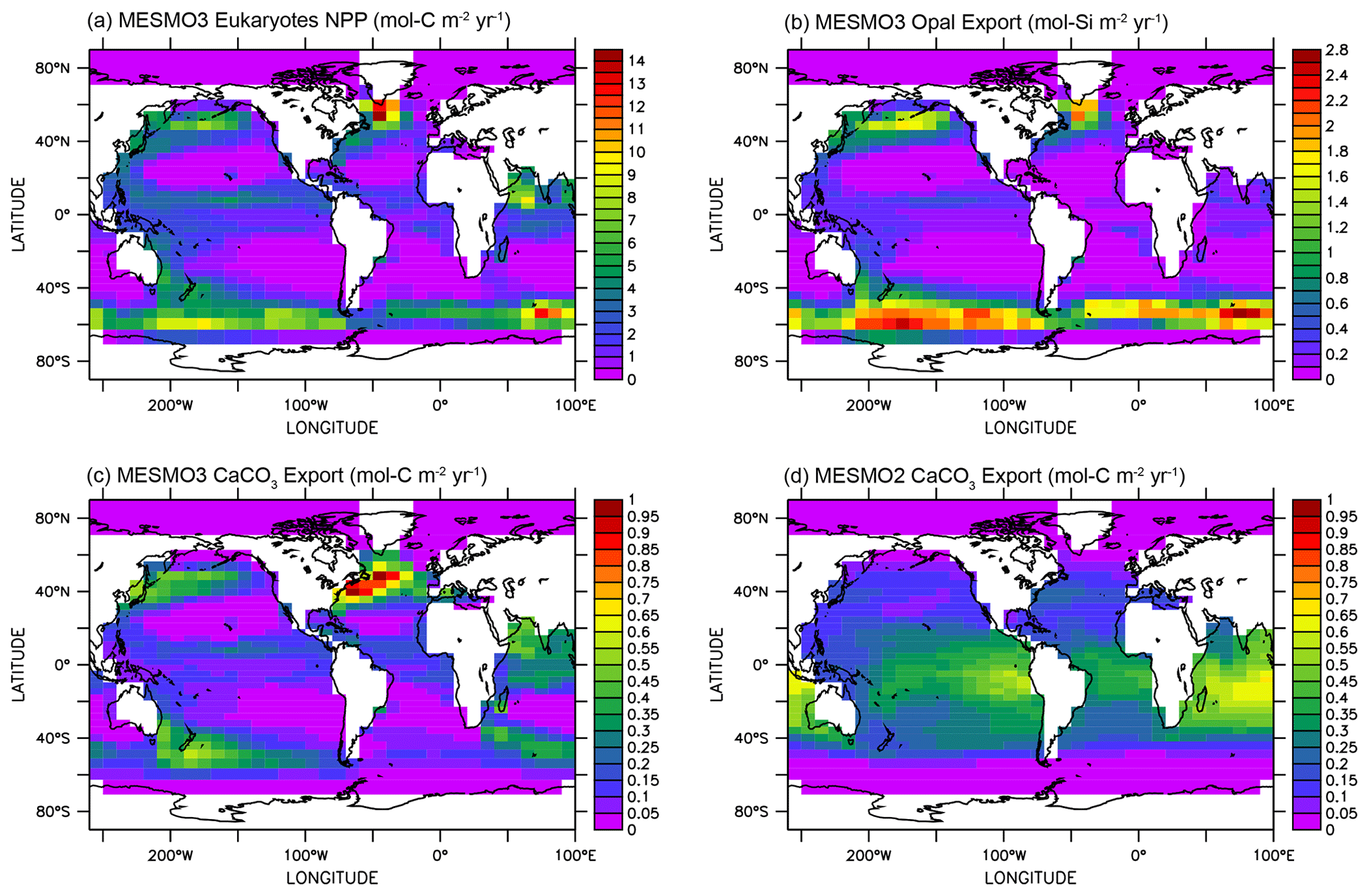
Figure 3 Eukaryote production in MESMO 3 and CaCO₃ export in MESMO 2. In MESMO 3, eukaryote NPP (a) is linked to both opal export (b) and CaCO₃ export (c) but the two export productions are differentiated by the residual nitrate potential growth (RNPG). Compare CaCO₃ export in MESMO 3 (c) to MESMO 2 (d) (unit: mol m⁻² yr⁻¹).

The global pattern of the mean C:P uptake ratio in the production layer is shown in Fig. 4. Consistent with observations (Martiny et al., 2013), the simulated C:P ratio of the phytoplankton community is elevated in the oligotrophic subtropical gyres and low in the eutrophic polar waters (Fig. 4a). The community C:P ratio exceeds 200 in the gyres and reaches as low as 40–50 in the Southern Ocean. The community C:P has contributions from both physiological effects (i.e., environmental drivers acting on each PFT's C:P ratio) and taxonomic effects (i.e., the shift in the community composition changes the weighting of each PFT's C:P ratio). Figure 4b shows that the community C:P is high in oligotrophic gyres because cyanobacteria and to a lesser extent diazotrophs dominate the community and their C:P ratio is high. Conversely, the community C:P is low in the polar waters because the eukaryotes dominate and their C:P ratio is low. For both eukaryotes and cyanobacteria, their C:P is high in oligotrophic subtropical gyres because PO₄ is low (Fig. 4c and d). This physiological effect is larger in eukaryotes than cyanobacteria because the former has greater sensitivity (i.e., larger sensitivity factor $s_{{\mathrm{PO}}_{\mathrm{4}}}^{\mathrm{P}:\mathrm{C}}$; see Eq. 5 and Table 2b). However, the cyanobacteria PFT's C:P ratio has an additional sensitivity to temperature (i.e., $s_T^{\mathrm{P}:\mathrm{C}}\ne \mathrm{0}$) that elevates their C:P in the lower latitudes. We do not show the C:P ratio for diazotrophs because it is very similar to that of cyanobacteria (Fig. 4b, d).

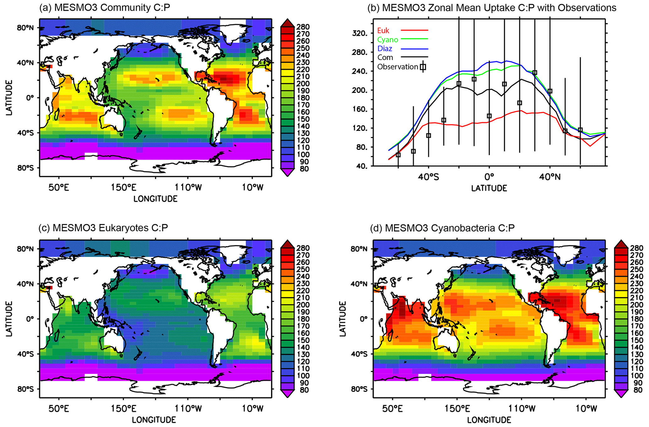
Figure 4 Uptake C:P ratio in the top 100 m in MESMO 3: (a) phytoplankton community C:P, (b) zonal mean C:P of all three PFTs and phytoplankton community, (c) eukaryote C:P, and (d) cyanobacteria C:P. The colors in (b) indicate community C:P (black), eukaryote C:P (red), cyanobacteria C:P (green), and diazotroph C:P (blue). In addition, (b) shows the mean range of observed C:P ratio binned by latitude (Martiny et al., 2013).

In order to gain more insights into the spatial patterns of the C:P ratio (Fig. 4), we examined the relationships between the C:P and C:N ratios and the four possible environmental drivers for eukaryotes and cyanobacteria (Fig. 5; again, diazotrophs are not shown). The red plots show that there is a causal relationship between the ratios and the drivers as formulated by the power law model (Eqs. 5 and 6). The black plots show the absence of a causal relationship. For example, the C:P ratio of both eukaryotes and cyanobacteria is strongly correlated with PO₄ because there is a causal relationship (Fig. 5a, b, shown in red). Similarly, the C:N ratio of the same two PFTs have a strong correlation with PO₄ (Fig. 5c, d in black), but there is actually not a causal relationship (i.e., $s_{{\mathrm{PO}}_{\mathrm{4}}}^{\mathrm{N}:\mathrm{C}}=\mathrm{0}$, Table 2b). The C:N-PO₄ correlation exists simply because the nutrients are well correlated. Similarly, because temperature and photosynthetically active radiation (PAR) tend to be correlated via latitude, the stoichiometry has a similar correlation to the two drivers. For example, cyanobacteria C:P has a strong correlation with both temperature and PAR (Figs. 5j, 4n), but only the temperature is a real driver. Figure 5 indicates which are the dominant drivers of the $\mathrm{C}:\mathrm{N}:\mathrm{P}$ ratio in MESMO 3. For the eukaryote C:P ratio, it is PO₄. For the cyanobacteria C:P ratio, the important drivers are temperature and PO₄. For the C:N ratio for both eukaryotes and cyanobacteria, NO₃ is more important than PAR. Figure 5 also serves to remind us that correlation does not indicate causation.

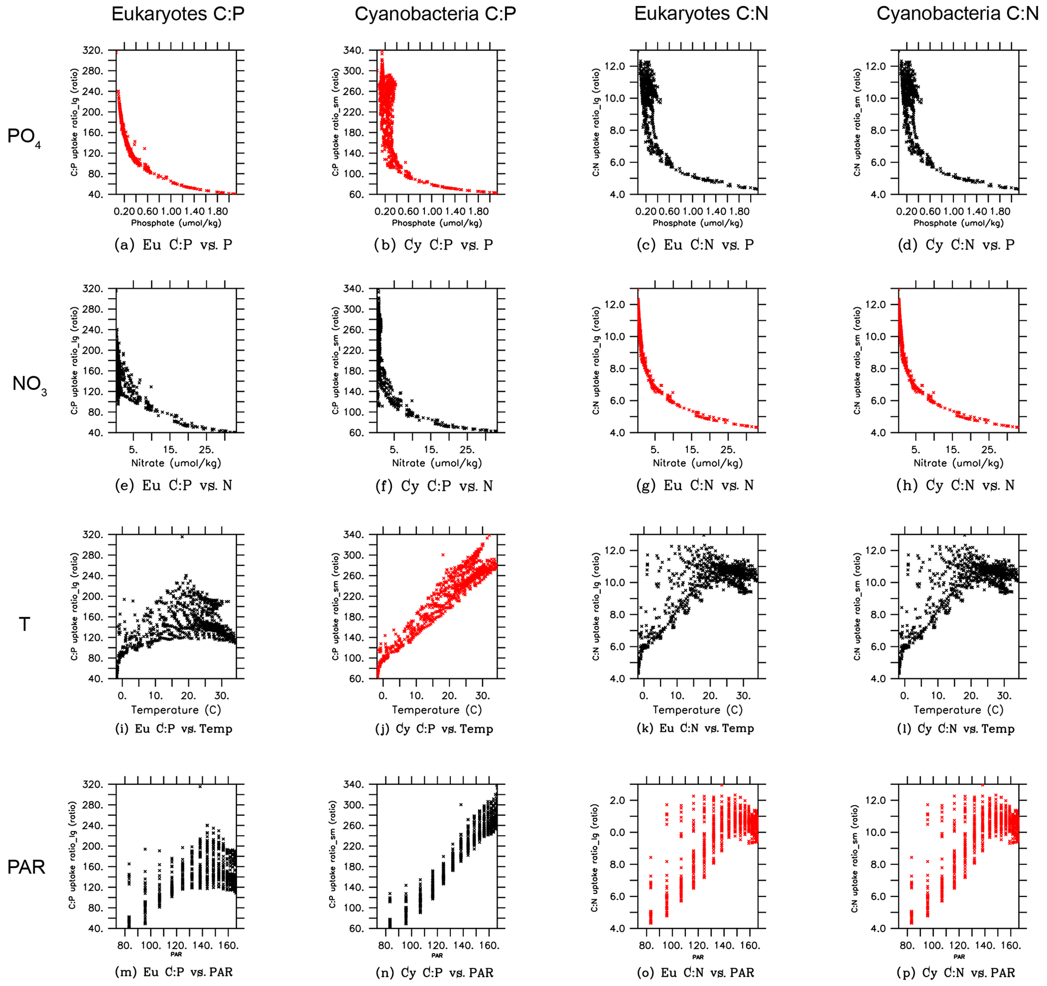
Figure 5 Scatterplots of surface ocean eukaryote and cyanobacteria C:P and C:N vs. environmental drivers in MESMO 3. Columns show the following data, from left to right, eukaryote C:P, cyanobacteria C:P, eukaryote C:N, and cyanobacteria C:N. Rows show the following data, from top to bottom, PO₄, NO₃, temperature, and PAR. Red indicates the causal relationship according to the power law formulation of flexible $\mathrm{C}:\mathrm{N}:\mathrm{P}$ ratio. PAR stands for photosynthetically active radiation in W m⁻².

Figure 6 shows the community C:P and C:N ratios plotted against the four environmental drivers. Unlike Fig. 5, which reflected the individual PFT's physiological response, Fig. 6 includes the effect of taxonomy as well. Still, the effects of PO₄ and temperature are clearly visible on the community C:P ratio. Both low [PO₄] and warmer waters are found in the lower latitudes, so the P frugality and temperature effects are additive. The effect of NO₃ on the community C:N ratio is also very clear, but the effect of PAR is not as clear. Thus, the overall physiological effects seen in the PFT-specific $\mathrm{C}:\mathrm{N}:\mathrm{P}$ are obvious in the community $\mathrm{C}:\mathrm{N}:\mathrm{P}$ ratio.

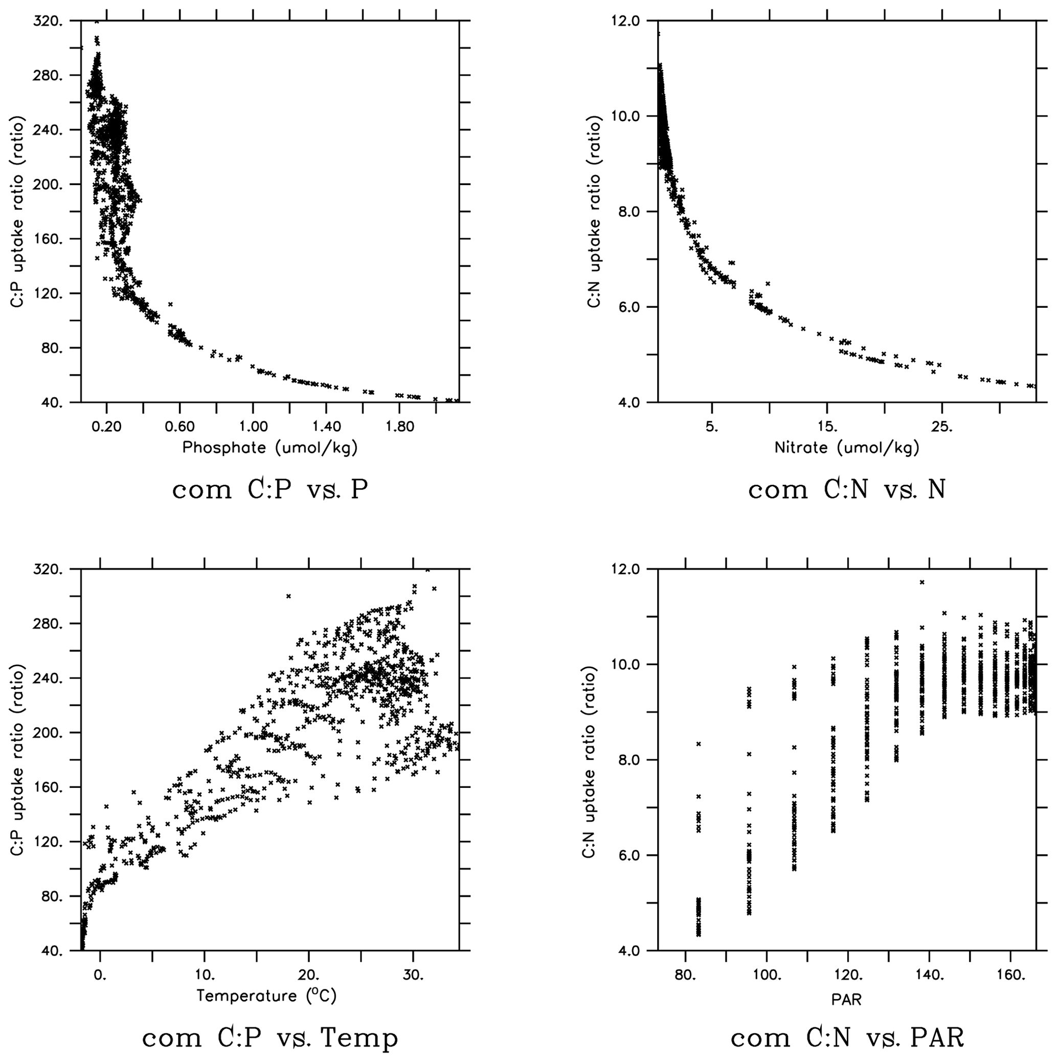
Figure 6 Scatterplots of surface ocean community C:P and C:N vs. environmental drivers in MESMO 3.

3.2 DOM_r-enabled MESMO 3

In MESMO 2, DOC_sl was a standard state variable. In MESMO 3, other forms of DOM are available as options. They are the semi-labile forms of DOM, i.e., DOP_sl, DON_sl, and DOFe_sl, and the refractory forms of DOM, i.e., DOC_r, DOP_r, and DON_r. MESMO 3 is not yet calibrated with respect to all the DOM variables, but here we demonstrate their potential use in future biogeochemical investigations by presenting steady state DOM results from the model experiment LV (experiment ID: 210310m). In this run, all three sinks of DOM_r are activated: slow background decay, photodegradation, and degradation in hydrothermal vents.

The experiment name LV stands for “literature values”. In LV, we use the literature values for the key DOM remineralization model parameters (Table 2d) and fDOM_r=0.01 (Hansell, 2013). All other model parameter values in the LV run are identical to the standard MESMO 3 model (Table 2). The black lines in Fig. 7 show the global mean vertical profiles of the total DOC (DOC_t = DOC_sl + DOC_r) with solid lines and DOC_r with a dashed line. Qualitatively, the simulated profiles are consistent with the observations, showing a near-uniform DOC_r concentration and a DOC_sl profile that rapidly attenuates with depth in the top few hundred meters (Hansell, 2013). However, the simulated values reach 130 µmol kg⁻¹ at the surface, which is approximately twice the observations. More typically, the observed DOC_r is 30–40 µmol kg⁻¹, and the observed DOC_sl attenuates with depth from 30–40 µmol kg⁻¹ near the surface. So their sum, which is represented by DOC_t, is approximately 60–80 µmol kg⁻¹ at the surface in observations.

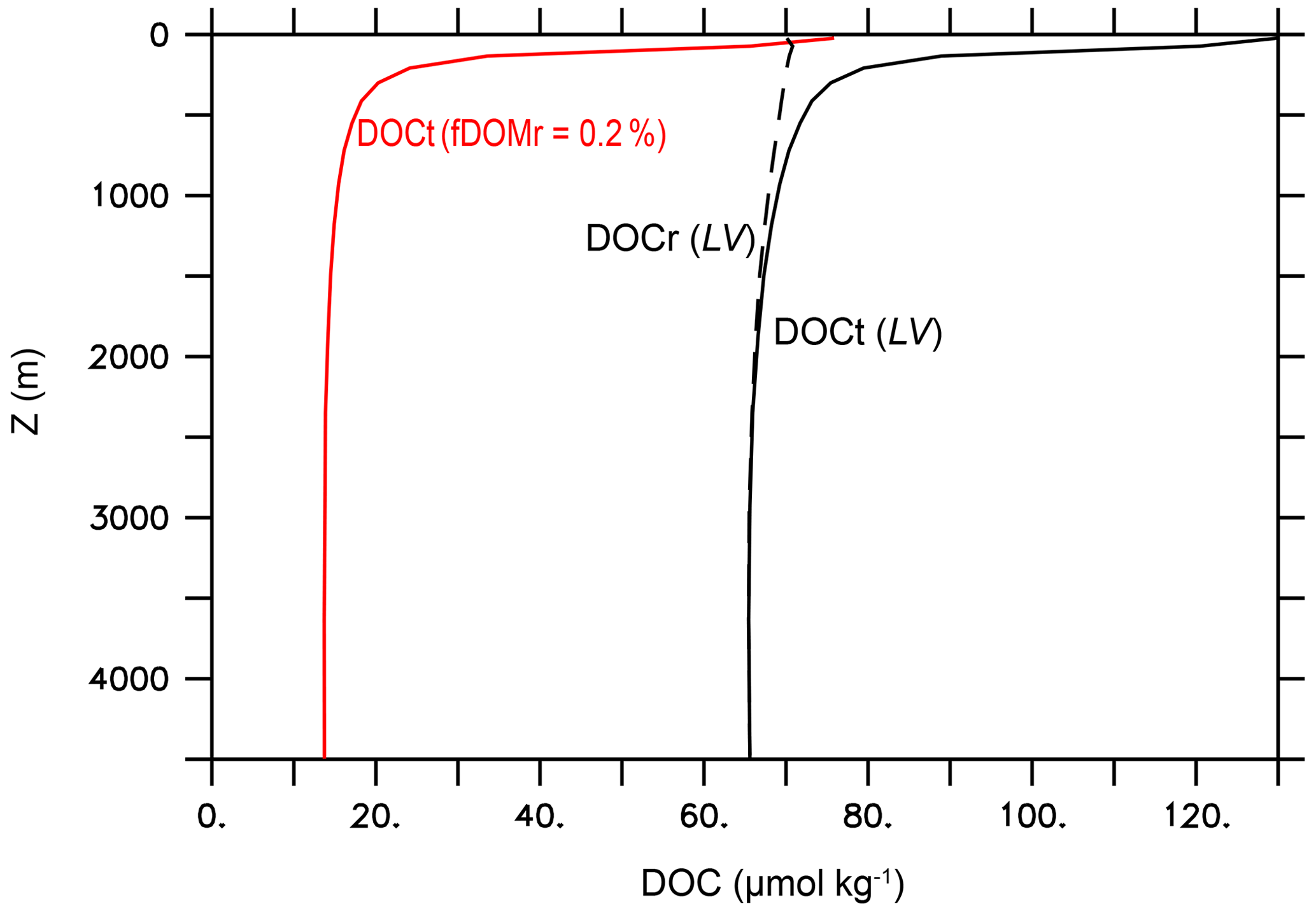
Figure 7 Global mean vertical profiles of DOC from the DOM_R-enabled MESMO 3. DOC_t (DOC_sl+DOC_r, black line) and DOC_r (dashed black line) from the LV run. The red line is DOC_t after reducing fDOM_r from 1 % in LV to 0.2 % (Experiment 210310o) (unit: µmol kg⁻¹).

Figure 8 adds a lateral perspective to Fig. 7. The rapid DOC_t attenuation in the vertical is strong in the lower latitudes where stratification is generally stronger. The transport of DOC_sl from the surface to deeper waters is evident in the high latitudes of the North Atlantic and the Southern Ocean. The DOC_t change in the deep ocean is limited.

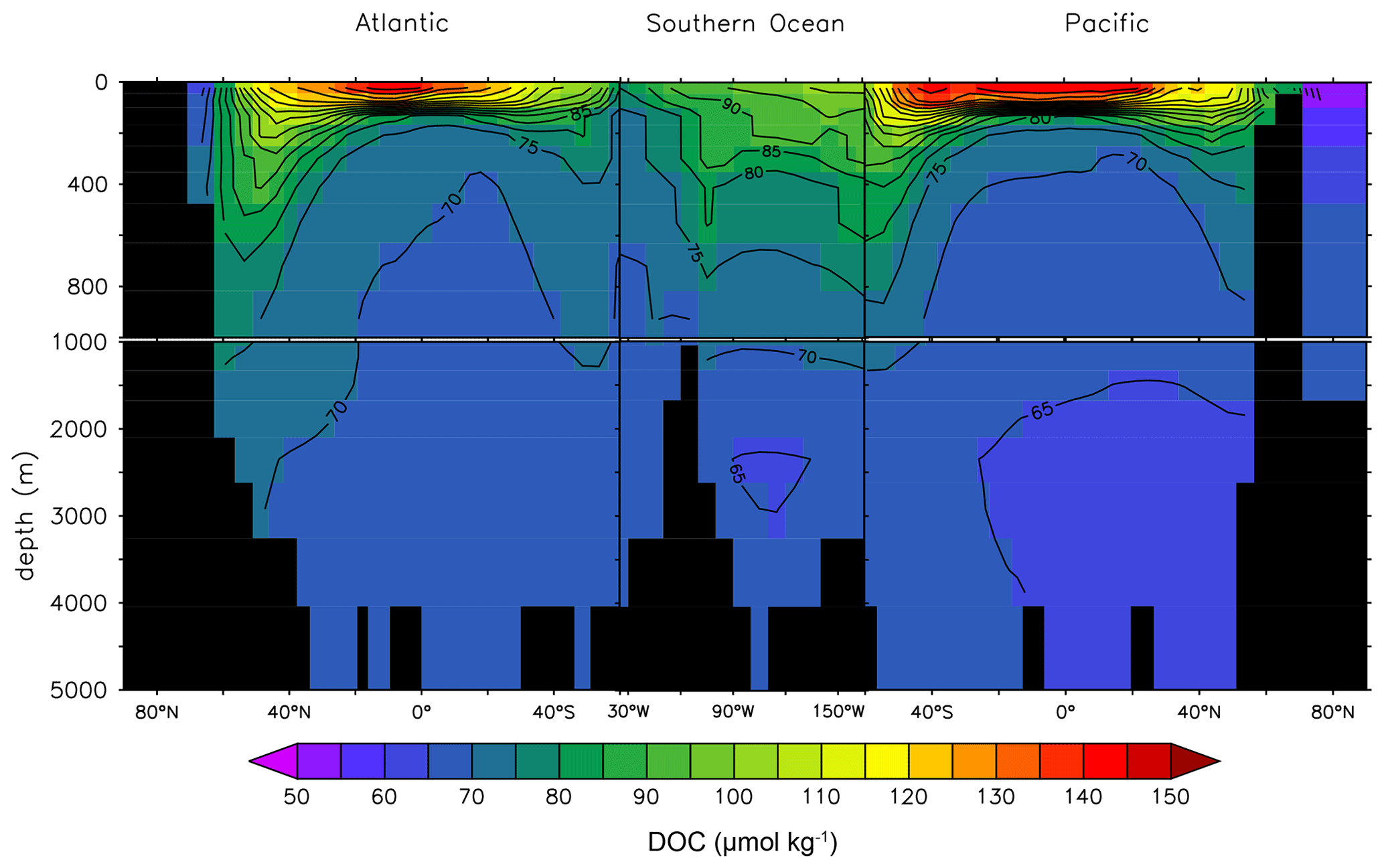
Figure 8 Global depth–latitude transect of DOC_t from the DOM_R-enabled MESMO 3 LV run. Transects are north–south along 25^∘ W in the Atlantic, east–west along 60^∘ S in the Southern Ocean, and north–south along 165^∘ E in the Pacific (unit: µmol kg⁻¹).

Observations of deep-ocean DOC_t indicate a reduction by 29 % or 14 µmol kg⁻¹ from the deep North Atlantic to the deep North Pacific (Hansell and Carlson, 1998). Figure 8 shows that the deep-ocean DOC_t gradient in LV is approximately 10 µmol kg⁻¹ from 70–75 µmol kg⁻¹ in the North Atlantic to < 65 µmol kg⁻¹ in the North Pacific.

The horizontal DOC_t distributions from the LV run can also be compared to a global extrapolation based on an artificial neural network (ANN) of the available DOC_t data (Roshan and DeVries, 2017). At the surface, the extrapolation indicates higher DOC_t concentrations in the subtropical gyres (Fig. 9a), while our simulation does not clearly delineate the gyres (Fig. 9c). In our model, fDOM is temperature-dependent and strongly controls the production of DOM. The surface DOC_t is thus more elevated in the lower latitudes. Interestingly, the ANN study diagnosed higher rates of DOM production in the subtropical gyres. Since the oligotrophic subtropical gyres have low NPP, the diagnosis would thus suggest that somehow fDOM is higher in the gyres. At depth, both the extrapolated and simulated DOC_t show a gradual decline in concentrations from the North Atlantic to the North Pacific (Fig. 9b, d). The highest deep DOC_t in the LV run is seen just south of Greenland, where convection occurs in the model.

Figure 9 Assessment of surface and deep-ocean DOC_t from the DOM_R-enabled MESMO 3 LV run. Data-derived DOC_t distributions in the top 100 m (a) and 2500–4000 m (b). Model-simulated DOC_t distributions in the top 100 m (c) and 2500–4000 m (d). Data-derived DOC_t are from Roshan and DeVries (Roshan and DeVries, 2017) (unit: µmol kg⁻¹).

Finally, we show that the deep-ocean radiocarbon aging is larger in DIC than in DOC_t in the model (Fig. 10). The North Pacific–North Atlantic Δ¹⁴C gradient is roughly −100 ‰ for DIC and −70 ‰ for DOC_t. The oldest DOC_tΔ¹⁴C is approximately −430 ‰ in the North Pacific. If ¹⁴C decay were the only mechanism of change along the path of the deepwater circulation, the Δ¹⁴C gradient should be quite similar between DIC and DOC_t, which are both dissolved phases and transported passively by the same circulation. The one potentially important difference is that the addition of the relatively young DI¹⁴C and DO¹⁴C to the deep ocean by the “deep POC split” (see Sect. 2.3). The addition impacts DOC_tΔ¹⁴C more than DIC Δ¹⁴C because DOC_t is 2 orders of magnitude lower in concentration than DIC.

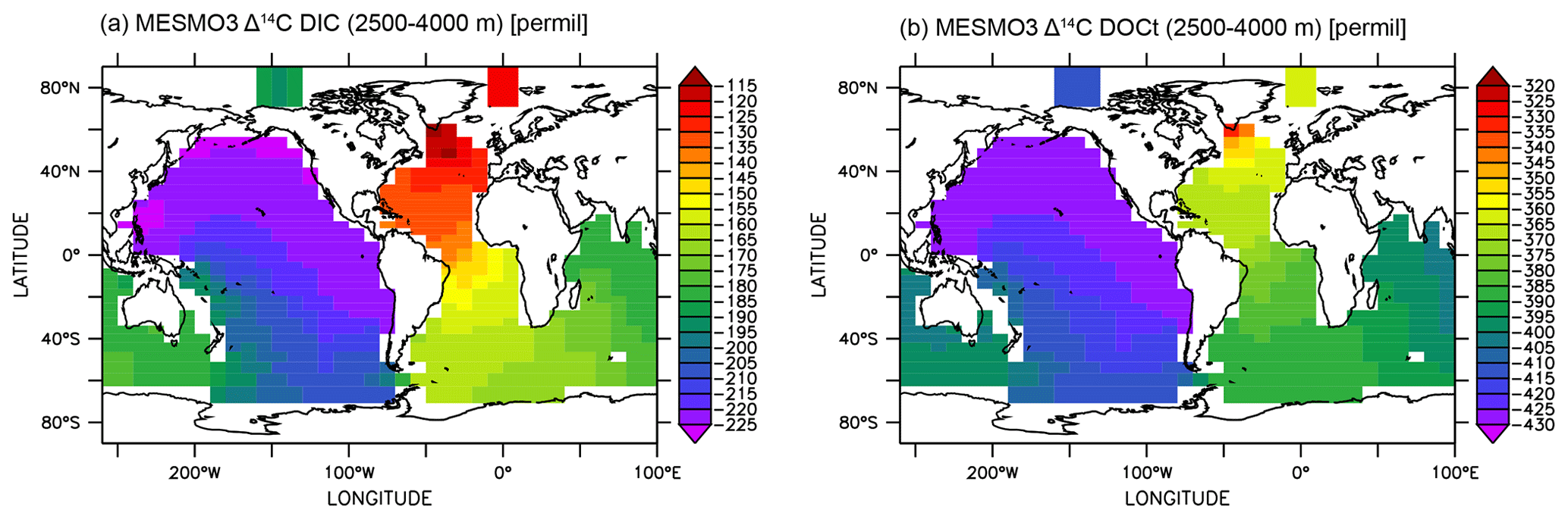
Figure 10 Δ¹⁴C of deep-ocean DIC (a) and DOC_t (b) from the DOM_R-enabled MESMO 3 LV run. Vertical average over 2500–4000 m water depth (unit: ‰).

In observations, the aging of DIC and DOC_t is reportedly similar in the Antarctic Bottom Water (below 4000 m) of the deep Pacific (Druffel et al., 2019). This may be explained by the fact that there would not be much deep POC split occurring so deep in the ocean. The North Pacific–North Atlantic Δ¹⁴C gradient, accounting for thermonuclear bomb ¹⁴C, may be as large as −100 ‰ for DOC_t (about −550 ‰ in the deep Pacific and −456 ‰ in the deep Atlantic) (Druffel et al., 2019). This gradient is not rigorously determined because there is not enough data to do an objective analysis. Therefore, the equivalent Δ¹⁴C gradient for DIC cannot be determined. However, the DIC Δ¹⁴C endmember values by inspection (about −250 ‰ in the deep Pacific and −70 ‰ in the deep Atlantic) (Matsumoto and Key, 2004) indicate a clearly larger Δ¹⁴C gradient for DIC than DOC_t as simulated by the experiment LV.

One lesson from the data–LV run mismatch in the overall DOC_t concentration (Fig. 7) and surface DOC_t pattern (Fig. 9) is that the parameter values from the literature do not fully capture the DOC cycle and/or that MESMO 3 is still lacking some important DOC process. In LV, the surface DOC_t is too high because DOC_r is too high, while DOC_sl is not unreasonable (Fig. 7). DOC_r is too high because there is too much DOC_r production (e.g., fDOM_r=1 % is too large), there is too little DOC_r degradation (e.g., one of the DOM decay mechanisms is too slow; Eq. 28 and Table 2d), or some combination of both. For example, fDOM_r is a key parameter that is not well constrained by observations. Had we used 0.2 % instead of 1 % for fDOM_r, the global mean surface DOC_t drops to 76 µmol kg⁻¹ (red line, Fig. 7), consistent with observations. For achieving a better surface DOC_t pattern, we may need a different formulation of fDOM that is, for example, negatively related to nutrient concentrations so that fDOM increases in the oligotrophic subtropical gyres (Roshan and DeVries, 2017).

Another lesson from the DOM modeling exercise is that it is important to simulate DOP_r reasonably well in order to preserve the favorable results we achieved in MESMO 3 with respect to biological production and the phytoplankton $\mathrm{C}:\mathrm{N}:\mathrm{P}$ ratio. We find that in the experiment LV, the global mean DOP_r concentration becomes steady at 0.45 µmol-P kg⁻¹. In observations, the mean DOC_r is about 40 µmol-C kg⁻¹ and the DOC_r:DOP_r ratio is estimated to be ∼ 1370:1 (Letscher and Moore, 2015), so DOP_r concentration should only be roughly 0.03 µmol-P kg⁻¹. Thus, the simulated DOP_r=0.45 µmol-P kg⁻¹ is an order of magnitude too high. Because there is more P in the form of DOP_r in LV, the oceanic inventory of PO₄ declines, causing a nearly 10 % drop in export production compared to the standard MESMO 3. In LV, the decline in the surface ocean PO₄ that accompanies the change in the PO₄ inventory acts on the phytoplankton physiology (i.e., P effect on C:P in Eq. 5), which leads to a large rise in the global mean phytoplankton community C:P export ratio from 113:1 to 127:1. The implementation of preferential remineralization of DOP (and DON) over DOC (Letscher and Moore, 2015) is one way to deal with the problem of too high DOP_r concentrations.

3.3 Large-scale patterns of N₂ fixation and denitrification

The modeled habitat of diazotrophs is concentrated in tropical and subtropical waters between 40^∘ S and 40^∘ N and limited by iron (Fig. 1e, f). Most noticeably in the North Pacific subtropical gyre, diazotrophs constitute ∼ 40 % of total NPP. The latitudinal extent of diazotrophs is mainly determined by surface nitrate availability and physical factors such as surface temperature and irradiance. Low nitrate availability in subtropical gyres gives diazotrophs a competitive advantage over small cyanobacteria. Warm temperature and high irradiance are also critical physical factors that drive the growth of diazotrophs in the model.

The modeled global depth-integrated N₂ fixation is 101 Tg N yr⁻¹ (Table 3), and this value falls well within the range of observational and geochemical constraints of 80–200 Tg N yr⁻¹ (Landolfi et al., 2018). In MESMO 3, N₂ fixation occurs in the North Pacific and mid-to-low latitudes of the Atlantic basin (Supplement Fig. S6), where diazotrophs are generally more abundant (Fig. 2e). The elevated N₂ fixation rate in the North Pacific, where nitrate limits eukaryotes and cyanobacteria (Fig. 2b, d), can be explained by the healthy growth of diazotrophs, which is not limited by N. In the subtropical and tropical Atlantic and the Indian Ocean, high N₂ fixation is driven by a elevated C:P and N:P ratio (Fig. 4), exemplified by low phosphate availability and warm surface temperature. This spatial pattern agrees with a recent inverse model study (Wang et al., 2019), which showed an elevated N₂ fixation rate in subtropical gyres.

Global water column denitrification is 101 Tg N yr⁻¹ (Table 3) and is equal to the global N₂ fixation because the model has reached steady state. Denitrification is restricted to the subpolar North Pacific (Fig. S6), where sub-surface oxygen concentration is significantly depleted (Fig. S3d). Enhanced denitrification in this region is in qualitative agreement with a previous modeling study (Bianchi et al., 2018), which showed the anaerobic niche due to particle microenvironments can significantly expand the hypoxic expanses in the North Pacific. However, the extent of denitrification in our model does not include the eastern equatorial Pacific and northern Indian oceans, which are important hotspots for denitrification (Codispoti, 2007; Deutsch et al., 2007). This issue is typical of coarse-resolution global ocean biogeochemistry models that lack spatial resolution in reproducing intense upwelling (Marchal et al., 1998; Najjar et al., 1992; Yamanaka and Tajika, 1997).

Finally, the ratio of the global inventories of NO₃ and PO₄ in MESMO 3 is just about 16 at steady state, consistent with observations (Gruber and Sarmiento, 1997). One key model parameter in this regard is the nitrate uptake half-saturation constant of diazotrophs, $K_{{\mathrm{NO}}_{\mathrm{3}}\mathrm{\_}\mathrm{Nfix}}$ in Eq. (58). A large value of $K_{{\mathrm{NO}}_{\mathrm{3}}\mathrm{\_}\mathrm{Nfix}}$ will make it hard for diazotrophs to obtain fixed N from NO₃, which would facilitate N₂ fixation and pushes up the global $\mathrm{N}/\mathrm{P}$ ratio. With a smaller value of $K_{{\mathrm{NO}}_{\mathrm{3}}\mathrm{\_}\mathrm{Nfix}}$, diazotrophs will more easily uptake NO₃, thus depressing N₂ fixation and lowering the global $\mathrm{N}/\mathrm{P}$ ratio.

4 Conclusions

MESMO 3, the third and latest version of MESMO, is comprehensively described here. With a fully flexible $\mathrm{C}:\mathrm{N}:\mathrm{P}$ ratio in three PFTs, a prognostic N cycle, and more mechanistic schemes of organic matter production and remineralization, MESMO 3 reflects the evolving and accumulating knowledge of the ocean biogeochemistry. The model thus remains an effective tool for investigations of the global biogeochemical cycles, especially over long timescales, given the model's computational efficiency. In particular, MESMO 3 holds promise for studying the marine DOM cycle. The optional features of MESMO 3 include the semi-labile and refractory pools of C, P, N, and Fe. The fact that the literature values regarding the present marine DOM cycle are unable to simulate key observations indicates an opportunity for MESMO 3 to contribute to an improved understanding of the marine DOM cycle.