Numerical study of the effects of initial conditions and emissions on PM_2.5 concentration simulations with CAMx v6.1: a Xi'an case study

A series of model sensitivity experiments was designed to explore the effects of different initial conditions and emissions in Xi'an in December 2016; Xi'an is a major city in the Fenwei Plain, which is a key area with respect to air pollution control in China. Three methods were applied for the initial condition tests: a clean initial simulation, a restart simulation, and a continuous simulation. In the clean initial simulation test, the C00, C06, C12, C18, and C24 sensitivity experiments were conducted to explore the effect of the intercepted time periods used. The results of these experiments showed that the fine particulate matter (PM_2.5) model performance was better when the start time of the intercepted time periods was delayed. For experiments C00 to C24, the absolute mean bias (MB) decreased from 51.07 to 3.72 µg m⁻³, and the index of agreement (IOA) increased from 0.49 to 0.86, which illustrates that the model performance of C24 is much better than that of C00. The R1120 and R1124 sensitivity experiments were used to explore the restart simulation and, in turn, the effect of the date of the first day of the model simulation. While the start times of the simulations were different, the simulation results with different start times were nearly consistent after a spin-up time period, and the results revealed that the spin-up time was approximately 27 h. For the continuous simulation test, the CT12 and CT24 sensitivity experiments were conducted. The start times of the intercepted time periods for CT12 and R1120 were the same, and the simulation results were almost identical. Based on the simulation results, CT24 showed the best performance of all of the sensitivity experiments, with the correlation coefficient (R), MB, and IOA reaching 0.81, 6.29 µg m⁻³, and 0.90 respectively. For the emission tests, an updated local emission inventory with construction fugitive dust emissions was added and was compared with the simulation results from the original emission inventory. The simulation with the updated local emissions showed much better performance for PM_2.5 modelling. Therefore, combining the CT24 method and the updated local emission inventory can satisfactorily improve the PM_2.5 model performance in Xi'an: the absolute MB decreased from 35.16 to 6.29 µg m⁻³, and the IOA reached 0.90.

1 Introduction

In recent years, severe air pollution has gradually become a major challenge in China and other developing countries (Wu et al., 2014; X. Li et al., 2017). China released a 3-year action plan for cleaner air in 2018, with efforts focused on areas including the Beijing–Tianjin–Hebei region, the Yangtze River Delta, and the Fenwei Plain. As a major city of the Fenwei Plain area, Xi'an is located in the Guanzhong Basin. The city is surrounded by the Qinling Mountains to the south, and the Loess Plateau extends to the north and west, which is not conducive to the dispersion of air pollutants. Xi'an has suffered severe air pollution in recent years because of its particular topography and rapid economic development (Zhang et al., 2002; Cao et al., 2012). Unfortunately, Xi'an is undergoing rapid development including urban construction activities that cause large construction fugitive dust emissions (Long et al., 2016).

Air quality modelling systems are an important tool for air pollution assessment and have evolved over three generations since the 1970s, driven by crucial regulations, societal and economic needs, and increasing high-performance computing capacity (Zhang et al., 2012). Various air quality models are widely used in the simulation and forecasting of pollutants, such as the Community Multiscale Air Quality (CMAQ) modelling system (Eder and Yu, 2006; Appel et al., 2017), the Comprehensive Air Quality Model with extensions (CAMx; ENVIRON, 2013), the Weather Research and Forecasting (WRF) model coupled with Chemistry (WRF-Chem; Grell et al., 2005), and the Nested Air Quality Prediction Modeling System (GNAQPMS/NAQPMS; Wang et al., 2006; Chen et al., 2015; Wang et al., 2017). To accurately analyse the apportionment of emission categories and contributions from different source regions for atmospheric pollution, many researchers have used the CAMx model with particulate matter source apportionment technology (PSAT) in different areas of China, including Beijing (Zhang et al., 2018), Tangshan (Li et al., 2013), the Pearl River Delta region (Wu et al., 2013), and the Yangtze River Delta region (Li et al., 2011). CAMx has shown satisfactory model performance for air pollution simulation (Panagiotopoulou et al., 2016).

The input files for the CAMx model include initial and boundary conditions, gridded and elevated point source emissions, and meteorological files (ENVIRON, 2013). Meteorology and emission inputs can cause high uncertainty in air quality models (Tang et al., 2010; Gilliam et al., 2015). Many studies have reduced the uncertainty of meteorology through refined physical parameterisations or other techniques, such as data assimilation (Sistla et al., 1996; Seaman, 2000; Gilliam et al., 2015; Li et al., 2019). A reasonable emission inventory is very important for the simulation accuracy of the air quality model. Numerous researchers have studied East Asian emissions (Kato and Akimoto, 1992; Streets et al., 2003; Ohara et al., 2007; Zhang et al., 2009) and have tried to construct emission inventories of particulate matter (PM) in China (Wang et al., 2005; Zhang et al., 2006). However, the absence of detailed information on China introduces uncertainty into these inventories (Cao et al., 2011). In recent years, an increasing number of researchers have focused on constructing and updating regional local emission inventories to improve model performance. Wu et al. (2014) improved model performance by adding more regional point source emissions and updating the area source emissions in villages and surrounding cities in Beijing. Based on that work, Yang et al. (2019) added local datasets to the emission inventory of the Guanzhong Plain (China), which was applied to simulate fine particulate matter (PM_2.5) concentrations using the CMAQ model in Xi'an. Numerous studies have indicated that construction dust emissions play an important role in air pollution, especially in urban areas (Ni et al., 2012; Huang et al., 2014; Wang et al., 2015). In our previous study, we created a particulate matter emission inventory from construction activities at the county level in Xi'an, which was based on an extensive survey of construction activities and was combined with two sets of dust emission factors for a typical city in northern China (Xiao et al., 2019).

However, few studies have investigated the effects of initial conditions on the simulation or prediction of PM_2.5 concentrations. Therefore, this study aimed to explore the effects of different initial conditions and emissions on model performance with respect to the simulation of PM_2.5 concentrations using the CAMx model. A series of model sensitivity experiments were designed using different initial conditions and emissions to find a suitable method for simulating PM_2.5 concentrations with a reasonable initial condition and emission inventory. In addition to Xi'an, other cities may apply a similar research method for simulating PM_2.5 concentrations in the future.

The remainder of this paper is organised as follows. Section 2 provides the model descriptions of the Weather Research and Forecasting–Sparse Matrix Operator Kernel Emissions–Comprehensive Air Quality Model with extensions (WRF-SMOKE-CAMx) model system, including meteorological fields, air quality model descriptions, the model domain, the emission inventory, and the processes. Section 3 presents the design of the sensitivity experiments for the different initial conditions and emissions. Section 4 discusses the model performance of the initial condition tests and emission tests with respect to simulating the PM_2.5 concentration in Xi'an. The conclusions are presented in Sect. 5.

2 WRF-SMOKE-CAMx model descriptions

In this study, the National Center for Atmospheric Research (NCAR) Weather Research and Forecasting (WRF v3.9.1.1) model (Skamarock et al., 2008), the Center for Environmental Modeling for Policy Development (CEMPD) Sparse Matrix Operator Kernel Emissions (SMOKE v2.4; Houyoux and Vukovich, 1999), and the Ramboll Environmental Comprehensive Air Quality Model with Extensions (CAMx v6.1; ENVIRON, 2013) were used to construct the air quality modelling system, as shown in Fig. 1. The WRF model provided the meteorological conditions for the SMOKE and CAMx models. The SMOKE model was used to process the emissions data and provide 4-D, model-ready gridded emissions for the CAMx air quality model.

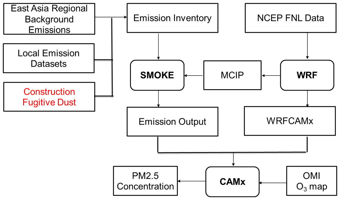
Figure 1 Framework of the WRF-SMOKE-CAMx model system in Xi'an. The Ozone Monitoring Instrument (OMI) O₃ map prepares ozone column input files for CAMx in order to improve the photolysis rate calculation. CAMx forecasted the air pollutant for the next 48 h.

2.1 Meteorological fields

For the WRF model configuration, we chose the Rapid Radiative Transfer Model (RRTM; Mlawer et al., 1997) and Dudhia scheme for long-wave and short-wave radiation options (Dudhia, 1989), WSM3 cloud microphysics (Hong et al., 2004), the Yonsei University (YSU) scheme (Hong et al., 2006), the Kain–Fritsch (new Eta) cloud parameterisation (Kain, 2004), and a five-layer thermal diffusion scheme (Dudhia, 1996). The meteorological initial and boundary conditions were derived from the National Centers for Environmental Prediction (NCEP) Final Analysis (FNL) Operational Global Analysis data, with a 1^∘ × 1^∘ spatial resolution and 6 h temporal resolution (National Centers for Environmental Prediction/National Weather Service/NOAA/U.S. Department of Commerce, 2000). The simulation was conducted between 20 November 2016 and 20 January 2017.

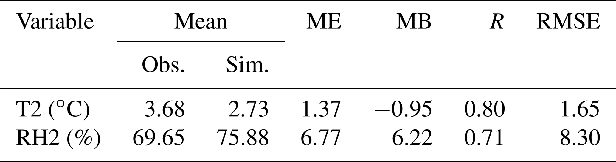
The simulated effect of daily average temperature (T2) and relative humidity (RH2) simulated by the WRF model in domain 3 were primarily validated by the observation data at seven monitoring stations in Xi'an; the station map is shown in Fig. 2. Some of the statistical parameters given in Appendix A were used to evaluate the model performance and are shown in Table 1; the time series is shown in Fig. 3. The mean error (ME), R, and root mean square error (RMSE) of the daily average T2 are 1.37 ^∘C, 0.80, and 1.65 ^∘C respectively, and the simulation shows a cooling bias of −0.95 ^∘C. The ME and RMSE of the daily average RH2 are 6.77 % and 8.30 % respectively. The correlation coefficient of the relative humidity is 0.71, which is reasonable. RH2 was slightly overestimated when the MB was 6.22 %.

In previous studies, Yang et al. (2019) used WRF to drive the CMAQ model for winter air quality in Xi'an, and the model evaluations for winter in 2016 showed that the MB, ME, R, and RMSE of T2 were −2.83 ^∘C, 2.83 ^∘C, 0.89, and 3.29 ^∘C respectively. The MB, ME, R, and RMSE of RH2 were 9.59 %, 10.63 %, 0.71, and 13.43 % respectively. Wu et al. (2010) used the fifth-generation NCAR/Penn State Mesoscale Model (MM5) as a meteorological driver for the Nested Air Quality Prediction Modelling System (NAQPMS). The statistical results showed that the MB and R of T2 were 2.1 ^∘C and 0.84, and those of RH2 were −15.8 % and 0.65 respectively. Using the same model configuration and monitoring sites, Yang et al. (2020) compared the simulated and observed wind speeds at an altitude of 10 m (W10) at Xi'an station from 20 November 2016 to 20 January 2017. As the results show, the W10 is underestimated. The MB of W10 is −0.14 m s⁻¹. The R of W10 is 0.63, indicating a good agreement between the observations and the model results.

Compared with previous studies, T2 and RH2 have lower MB, ME, and RMSE values. The R of T2 is slightly lower than in previous studies, whereas the R of RH2 is higher. Thus, the meteorological simulation in this study is reasonable.

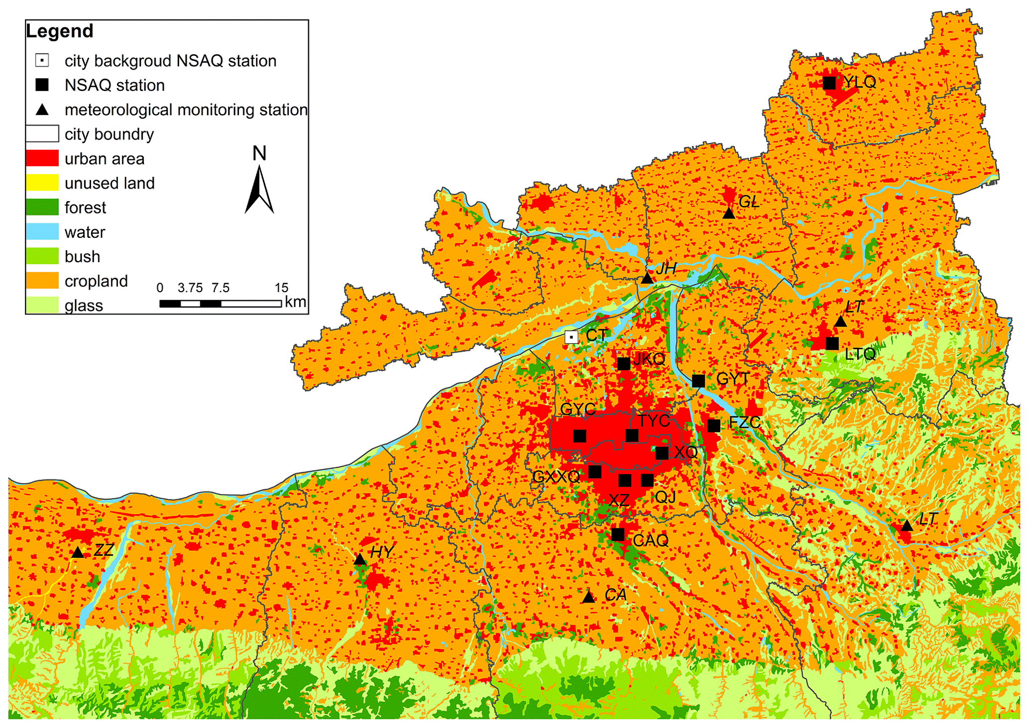
Figure 2 Map of the meteorological and air quality monitoring network in Xi'an. The triangles are the meteorological monitoring stations. The square with a dot in it is the city background station, and the black squares are the National Standard Air Quality (NSAQ) observation stations: Gaoyachang (GYC), Xingqing (XQ), Fangzhicheng (FZC), Xiaozhai (XZ), Tiyuchang (TYC), Gaoxinxiqu (GXXQ), Jingkaiqu (JKQ), Qujiang (QJ), Gaoyuntan (GYT), Changanqu (CAQ), Yanliangqu (YLQ), Lintongqu (LTQ), and Caotan (CT).

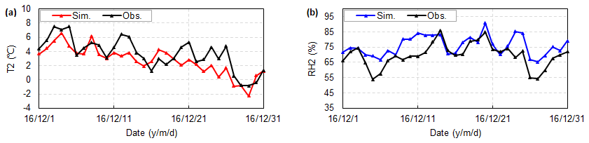
Figure 3 Time series plots of (a) daily average simulated and in situ 2 m temperature (T2) and (b) simulated and in situ 2 m relative humidity (RH2) at the Xi'an station.

Table 1 Verification statistics of daily temperature at a height of 2 m (T2), and relatively humidity at a height of 2 m (RH2). “Obs.” denotes observations, and “Sim.” denotes simulated values.

2.2 Air quality model descriptions

CAMx is a state-of-the-art air quality model developed by Ramboll Environ (http://www.camx.com, last access: 19 December 2020). In this study, the piecewise parabolic method (PPM) advection scheme (Colella and Woodward, 1984) was used for horizontal diffusion, and the K-theory was selected for vertical diffusion. The Regional Acid Deposition Model (RADM-AQ; Chang et al., 1987) scheme was chosen as the aqueous-phase oxidation, ISORROPIA (Nenes et al., 1999) was selected as the inorganic aerosol thermodynamic equilibrium, CB05 (Yarwood et al., 2005) was chosen as the gas-phase chemical mechanism, and the Euler backward iterative (EBI) solver with Hertel's solutions (Hertel et al., 1993) was used in the model system. The resistance model for gases (Zhang et al., 2003) and aerosols (Zhang et al., 2001) in the dry deposition module and the scavenging model for gases and aerosols (Seinfeld and Pandis, 1998) in the wet deposition module were utilised in this study. The CAMx model forecasted the next 48 h of PM_2.5 concentrations in the clean initial simulation test, and this is described in Sect. 3.1. On the first day, CAMx used the results from ICBCPREP, which can prepare a simple, static CAMx initial condition (IC) and boundary condition (BC). On the following days, it used the various initial conditions of the sensitivity experiments.

2.3 Model domain

Three nested domains were designed for the WRF model (Fig. 4), with respective horizontal resolutions of 27 km×27 km (D1), 9 km×9 km (D2), and 3 km×3 km (D3). The largest domain (D1) covers most parts of China, and the second domain (D2) includes Shaanxi Province, Shanxi Province, Henan Province, and the inner domain (D3), which focuses on the 11 cities in the Fenwei Plain, including Xi'an. CAMx only has one domain, and the settings are the same as those in the D3 domain when focusing on Xi'an as one sensitivity test area for initial conditions and emissions. To reduce the boundary effects, the CAMx model cuts down the outermost grid of the WRF model and uses the variable of the centre grid in the WRFCAMx module. Thus, the CAMx model had three grid cells smaller than the WRF model in the D3 domain. The vertical resolution of WRF was 37 layers from the ground to 5 hPa at the top, and 14 layers were extracted by the WRFCAMx module, which can convert the WRF output files into the CAMx model data format.

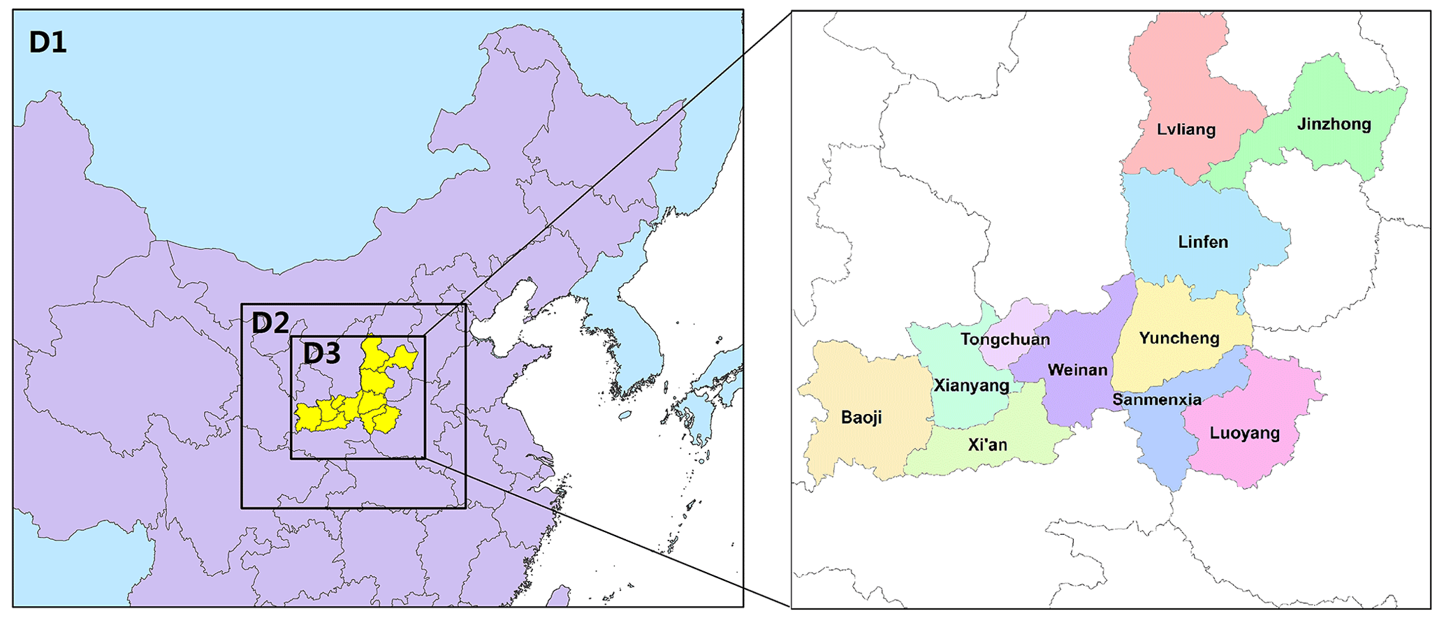
Figure 4 The three nested model domains with respective horizontal resolutions of 27 km×27 km (D1), 9 km×9 km (D2), and 3 km×3 km (D3) in the WRF-CAMx modelling system. D1 covers most parts of China, with 148×121 grids, and D2 includes Shaanxi, Shanxi, and Henan provinces. The inner domain covers Fenwei Plain, including Xi'an.

2.4 Emission inventory and processes

SMOKE version 2.4 (Houyoux and Vukovich, 1999) was used to improve the Fenwei emissions, especially Xi'an local emissions, and to provide gridded emissions for the CAMx model in this study. Based on the emission inventories of a previous study (Yang et al., 2019), this study updated the local emission inventories by adding the emission contribution of PM_2.5 from construction fugitive dust in Xi'an. Thus, the emission inventories in this study include the following:

1. The regional emissions in East Asia and the local emissions in the Guanzhong Plain were obtained from Wu et al. (2014) and Yang et al. (2019). Major industrial emissions were slightly adjusted according to the annual report in this study. The emission inventory at the city level is presented in Table 2.

2. Construction fugitive dust emissions in Xi'an, based on survey data from the construction projects shown in Fig. 5, were collected in a previous study (Xiao et al., 2019) and were indicated as a “local area source”. This is a new dataset at the county level and was updated in 2017. The basic data include the location and area of each construction project. We also replenished the missing construction data and corrected erroneous information using Google Earth and other geographic information tools in order to obtain more accurate location information. According to statistics, there were 1595 construction projects in Xi'an in 2017, comprising 86.1 km² of total construction area. The construction area in the main urban region (Xincheng, Beilin, Lianhu, Yanqiao, Weiyang, and Yanta) was about 62.2 km², comprising 7.5 % of the total main urban area. The distribution of the construction fugitive dust emissions in Xi'an is shown in Fig. 6.

We employed the statistical allocation approach to generate gridded area source emissions, which were used to allocate the total emissions to each horizontal model grid according to the related spatial factors. In this study, the LandScan 2015 Global Population Database (Dobson et al., 2000) was used as a population spatial factor to allocate the emissions. For the construction fugitive dust emissions, we used the area of each construction project as the weight in the surrogate calculation and allocated the input construction project data to the target polygons (map of the administrative division in Xi'an at the county level) based on the weighted spatial overlap of the input data and target polygons. The spatial results provide the SMOKE model as a spatially allocated factor. The horizontal and vertical allocation of point source emissions were assigned from their longitude–latitude coordinates and the Briggs algorithm (Briggs, 1972, 1984) respectively. The temporal variation and chemical species allocation were based on profile files in the SMOKE model.

As shown in Table 2, the NO_x emissions ranged from 352.0 to 758.5 kt yr⁻¹ between 2008 (in Zhang et al., 2009) and 2017 (in this study). For PM₁₀ emissions in Shaanxi Province, the emissions also increased from 474.0 to 830.0 kt yr⁻¹. The PM₁₀ emissions in this study are higher than values in other studies due to the inclusion of construction fugitive dust. Other emission species, such as NO_x, SO₂, NH₃, volatile organic compounds (VOCs), and CO, were slightly higher in this work than in previous studies.

Table 2 Emission of major anthropogenic species in Shaanxi Province (unit: 10³ t yr⁻¹).

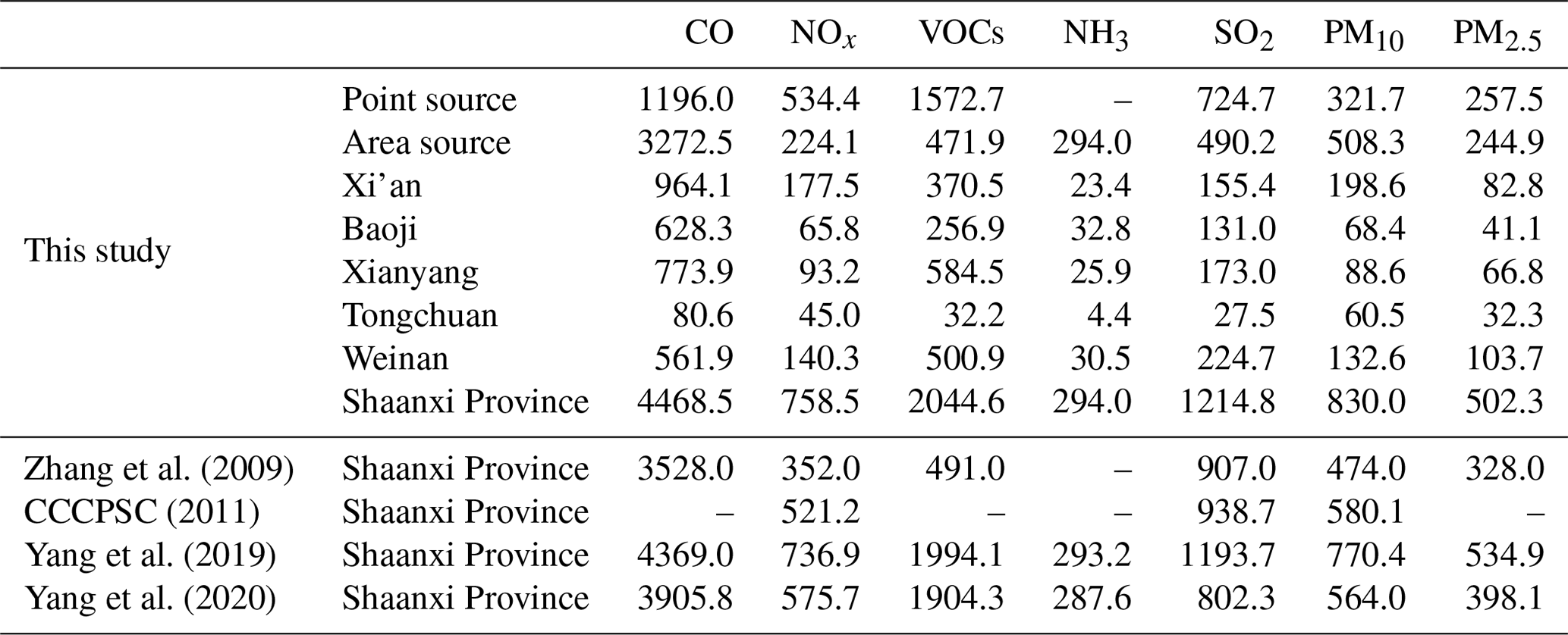
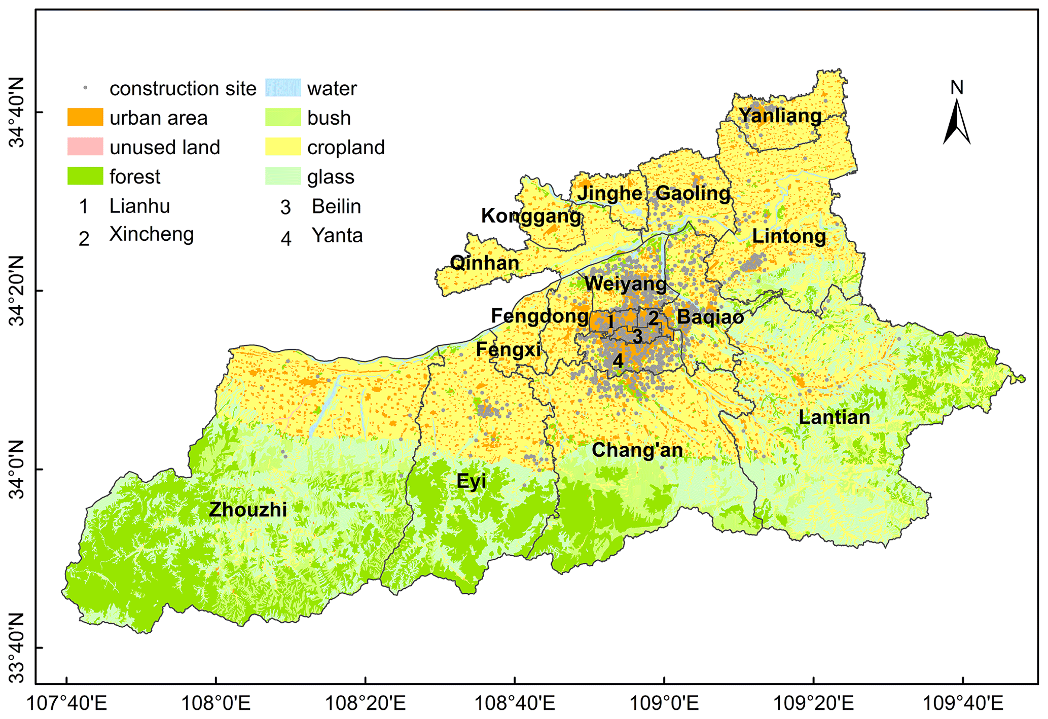
Figure 5 Spatial distribution of construction sites in Xi'an. Grey dots indicate the construction sites. The base map shows the types of land use (Xiao et al., 2019).

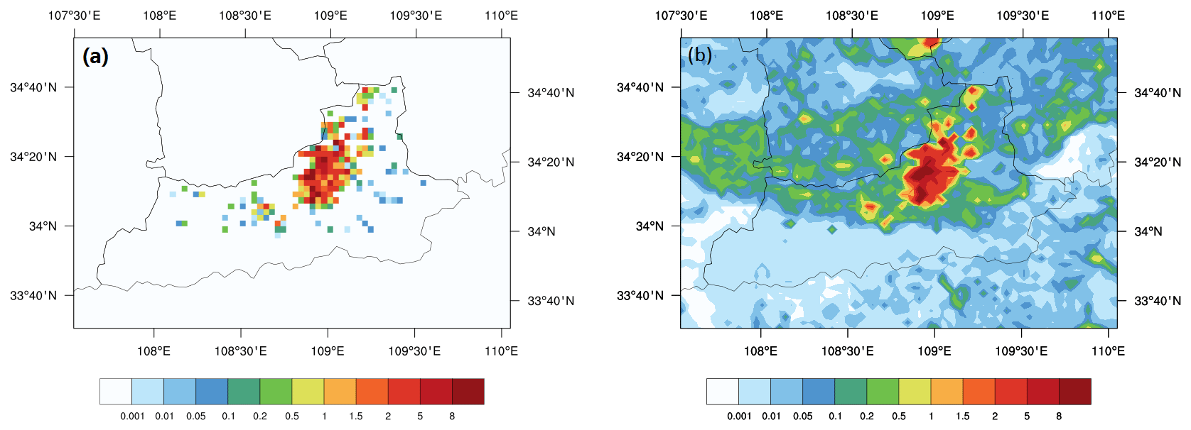
Figure 6 Spatial distribution of PM₁₀ emissions in Xi'an and its surrounding area. (a) Construction fugitive dust in Xi'an only. (b) All surface PM₁₀ emissions in Xi'an. The grid size is 3 km×3 km. (Unit: g km⁻² s.)

3 Design of the sensitivity experiments

A set of model sensitivity experiments using different initial and emission conditions were designed in this study. Three methods were applied for the initial condition tests: using the clean initial condition files as a clean initial simulation, using the restart files as a restart simulation, and a continuous simulation. For the emission tests, we compared the simulation results using the original emission inventory and those using the updated local emission inventory with construction fugitive dust emissions. The configurations of the sensitivity experiment simulations are shown in Table 3, and the time period for each initial condition experiment is shown in Fig. 7.

3.1 Initial condition (ICON) test using the clean initial condition files

The ICBCPREP module used a clean-troposphere vertical profile to generate the initial concentration fields for each day for the simulation using the clean initial condition files. The output files from CAMx were initialised at 13:00 UTC. The CAMx model forecasted the next 48 h of PM_2.5 concentrations in each simulation cycle. By extracting data from simulated results based on different time periods (0–24, 6–30, 12–36, 18–42, and 24–48 h respectively), as shown in Fig. 7a, we conducted the C00, C06, C12, C18, and C24 sensitivity experiments to explore the influence of different time periods on the simulation of PM_2.5. For the C00 sensitivity experiment, the data from the first 24 h of the output file were cut and merged for analysis. For C06, the first 6 h of data was spin-up time; we cut and merged the data from 19:00 to 18:00 UTC on the second day. C12, C18, and C24 used the same method to extract and merge data, and their spin-up times were the first 12, 18, and 24 h of data respectively.

3.2 ICON test using the restart files

The meteorological data for the 12–36 h period were cut to estimate the PM_2.5 concentrations by restarting the simulation of the CAMx model. The ICBCPREP module also used clean initial concentration fields at the beginning of the first simulation day to use the restart files. The gridded 3-D instantaneous concentrations of all species on all grids were written at the end of the simulation to allow for a model restart. ICON then used the 24 h forecast results from the day before as the initial conditions for the following days, as shown in Fig. 7b. The first day of the simulation started at 12:00 UTC, and the following days started at 00:00 UTC. To explore how long the spin-up time should be to eliminate the error caused by the initial value, the R1120 and R1124 sensitivity experiments were set at the first day of the model simulation, which began on the 20 and 24 November 2016 respectively.

3.3 ICON test using the continuous simulation

For the continuous simulation, the CT12 and CT24 sensitivity experiments were set at the start time of the intercepted time periods, which began at 00:00 UTC and 12:00 UTC respectively, as shown in Fig. 7c. For CT12, the meteorological data from the 12–36 h period were cut and merged into one file. The 24–48 h period was cut and merged for CT24. We also built the continuous emission files using the SMOKE model. During the simulation, there was no interruption, and a long-term sequence simulation result for each start time was finally generated.

3.4 Emission test using different emission inventories

Based on the initial condition tests, we selected the best method to perform the emission sensitivity experiments. We compared the simulation results of the original emission inventory (Enc sensitivity experiments) and the updated local emission inventory with the construction fugitive dust emissions (Ec sensitivity experiments) for the emission tests.

Table 3 The simulation experiment configurations. C00–C24, R1120, R1124, CT12, and CT24 were used to investigate the impact of simulation methods, the start time, and the extracted time period. The impact of different emission inventories was investigated using Ec and Enc. C, R, and CT in the “Method” column represent the clean initial condition simulation methods, the restart simulation, and the continuous simulation; nc and c in the “Emission inventory” column represent the original emission inventory and the updated local emission inventory with the construction fugitive dust emissions respectively.

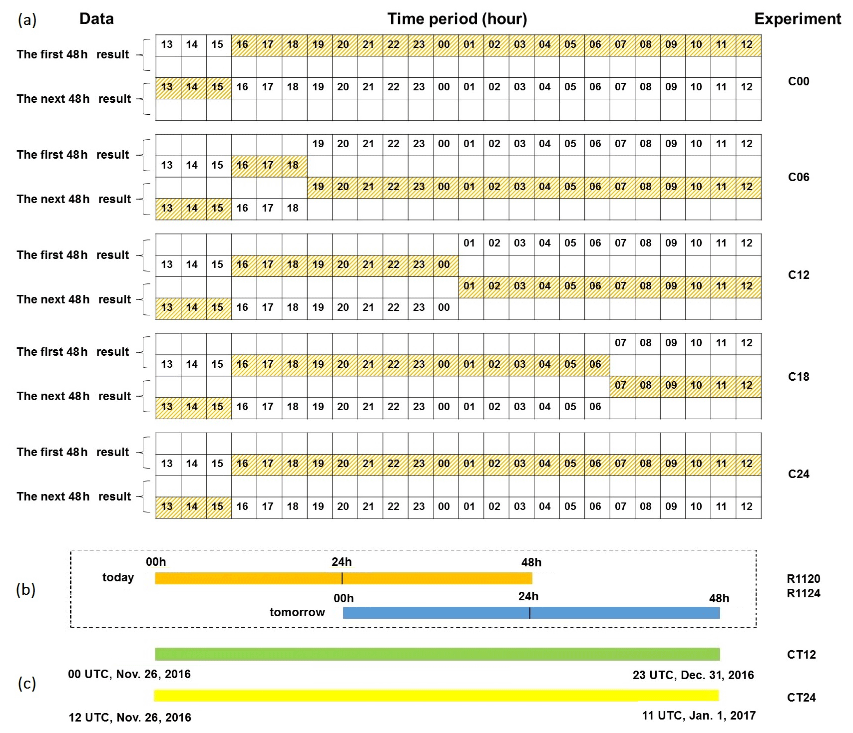
Figure 7 Time period for each initial condition experiment. Panel (a) shows the time period for the clean initial condition experiments (denoted using C). The output files from CAMx were initialised at 13:00 UTC every day, and the CAMx model forecasted the next 48 h of PM_2.5 concentrations in each simulation cycle. The C00, C06, C12, C18, and C24 sensitivity experiments extract different time periods (0–24, 6–30, 12–36, 18–42, and 24–48 h respectively) in each output file as valid data, represented by the grids with a number in them. Each grid represents an hour, and the numbers in the grids indicate the hours of the data. The grids with numbers in them represent the valid time period for each output file. The 24 h of data from a day is cut and merged from 16:00 UTC in the valid time period of each output file to analyse from 00:00 Beijing time (16:00 UTC) every day. The shaded grids represent the data for 1 single day. Panel (b) shows the time period for the restart experiments (denoted using R). The meteorological data from the 12–36 h period were extracted to estimate the PM_2.5 concentrations by restarting the simulation. The first day of the simulation starts at 12:00 UTC, and the following days start at 00:00 UTC. Panel (c) shows the time period for the continuous simulation experiments (denoted using CT). The meteorological data from the 12–36 h period were cut and merged into one file for CT12, and data from the 24–48 h period were cut and merged for CT24.

4 Results and discussion

In this study, we collected the observations in December 2016 and evaluated the model performance and improvement. Hence, the model ability was evaluated using both the meteorological field and daily PM_2.5 simulations in Xi'an.

4.1 Model performance for the initial condition tests

There are 13 NSAQ stations in Xi'an, which are marked using squares in Fig. 2. Nine stations are in urban Xi'an, including GYC, XQ, FZC, XZ, TYC, GXXQ, JKQ, QJ, and GYT. Three stations are located in suburban towns, including CAQ, YLQ, and LTQ. The CT station is the city background station, which is located in an urban area in northern Xi'an.

4.1.1 Sensitivity experiments using clean initial condition files

A Taylor nomogram (Taylor, 2001; Gates et al., 1999) was used to evaluate the accuracy of the simulated PM_2.5 daily concentrations for NSAQ stations that were used for the sensitivity experiments with clean initial condition files, as shown in Fig. 8. There are three statistical parameters to evaluate model accuracy in the Taylor nomogram (Taylor, 2001; Gates et al., 1999; Chang and Hanna, 2004): the correlation coefficient (R), the normalised standard deviation (NSD), and the normalised root mean square error (NRMSE). The C00, C06, C12, C18, and C24 sensitivity experiments are shown using different coloured symbols. We randomly selected three stations in urban Xi'an, two stations in county towns and a background station, to show the simulation results. “AVG” refers to the average of 13 NSAQ stations.

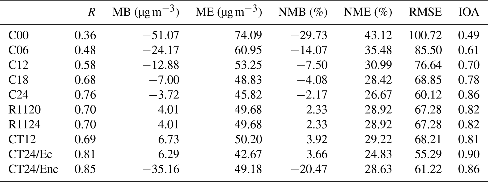
As shown in Fig. 8, R is between 0.36 and 0.76 for the C00, C06, C12, C18, and C24 sensitivity experiments. The R value is the largest and best for C24 for all NSAQ stations, and is the lowest for C00. The NRMSE, which measures the distance from the marker to the REF (a perfect simulated result for the air quality model) in the Taylor nomogram, is the smallest and best for C24 and is the longest for C00. Regarding the NSD, most NSAQ stations have similar regularity – that is, the NSD values from C00 to C24 become closer to one. The other statistical parameters are presented in Table 4. From the C00 to C24 experiments, the absolute mean bias (MB) and the mean error (ME) decreased from 51.07 to 3.72 µg m⁻³ and from 74.09 to 45.82 µg m⁻³ respectively. The absolute normal mean bias (NMB) and the normal mean error (NME) decreased from 29.73 % to 2.17 % and from 43.12 % to 26.67 % respectively. The index of agreement (IOA) increased from 0.50 to 0.8. In general, the model performance is better for C24 than for the other sensitivity experiments in the clean initial simulation tests.

Figure 8 Taylor nomogram for modelled and observed daily averaged PM_2.5 concentrations for the sensitivity experiment using the clean initial condition files. “AVG” refers to the average of 13 NSAQ stations. The C00, C06, C12, C18, and C24 sensitivity experiments are represented using different coloured symbols. According to Chang and Hanna (2004), REF represents a perfect simulated result for the air quality model.

4.1.2 Sensitivity experiments using restart files

The R1120 and R1124 sensitivity experiments were set at the date of the first day of the model simulation in order to explore the restart simulation. Starting from 12:00 UTC on 24 November, the PM_2.5 concentration simulation results of R1120 and R1124 are shown in Fig. 9. At first, the results of the two sensitivity experiments are very different; the two lines are then gradually fitted until 16:00 UTC on 25 November. After 16:00 UTC (on 25 November), the two lines fit almost completely. Therefore, a spin-up time of 27 h can eliminate the error introduced by the initial field for the PM_2.5 concentrations in the CAMx model.

As shown in Table 4, the model performance of the R1120 and R1124 sensitivity experiments is similar in December 2016. The R value between the observations and simulations for R1120 and R1124 was 0.70. The mean bias (MB) and mean error (ME) were 4.01 and 49.68 µg m⁻³ respectively. The normal mean bias (NMB) and normal mean error (NME) were 2.33 % and 28.92 % respectively. The root mean square error (RMSE) was 67.28, and the IOA reached 0.82.

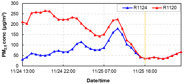
Figure 9 The time series of hourly simulated PM_2.5 concentrations using the restart files during a spin-up time period. The red and blue lines represent the R1120 and R1124 model sensitivity experiments respectively. The starting day of the model simulation for R1120 was 20 November 2016, and the starting day of the model simulation for R1124 was 24 November 2016.

4.1.3 Sensitivity experiments using the continuous simulation

For the continuous simulation, sensitivity experiments were conducted with CT12 and CT24. Although the CT12 and R1120 sensitivity experiments use different methods to generate the initial concentration fields, the start times of the intercepted time periods for the two experiments were the same. The PM_2.5 concentrations of CT12 and R1120 are presented in Fig. 10. As shown in Fig. 10, the points lie very close to the perfect line “y=x”, which indicates that the simulation results of CT12 and R1120 were nearly identical.

The model starting times of the CT12 and CT24 sensitivity experiments are 26 November at 00:00 UTC and 26 November at 12:00 UTC respectively. The concentration accumulation of CT24 was 12 h higher than that of CT12. As shown in Fig. 11, there is an air pollution peak in December 2016, for which CT24 matches better than CT12. The statistical parameters of CT12 and CT24 are presented in Table 4. The mean bias (MB) and mean error (ME) of the CT24 results were 6.29 and 42.67 µg m⁻³ respectively, which are slightly better than the CT12 results. The root mean square error (RMSE) of the CT24 results is 68.21, which is also slightly better than the CT12 results. From CT12 to CT24, the R and IOA increased from 0.69 to 0.81 and from 0.81 to 0.90 respectively. Thus, the sensitivity experiments with CT24 show better model performance than CT12.

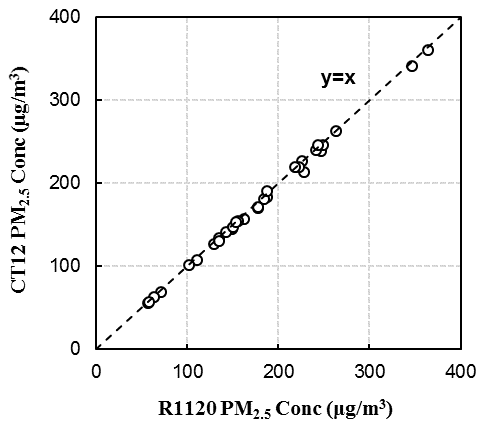
Figure 10 Scatter diagram of the R1120 and CT12 experiments for PM_2.5 concentrations. The “y=x” line represents that the simulated value from R1120 is the same as CT12.

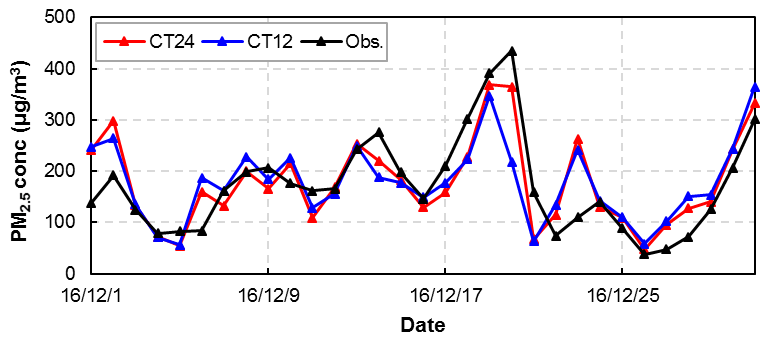
Figure 11 Time series of the daily PM_2.5 concentrations for the continuous simulation for Xi'an. The black line represents observations, and the blue and red lines show simulated data starting on 26 November at 00:00 UTC and on 26 November at 12:00 UTC respectively.

4.2 Model performance for the emission tests

A Taylor nomogram for the modelled and observed daily averaged PM_2.5 concentrations for all initial condition sensitivity experiments is shown in Fig. 13. The red symbols indicate the sensitivity experiment using the clean initial condition files, the blue symbols represent the sensitivity experiments using the restart files, and the brown symbols show the continuous simulation sensitivity experiments. One experiment is shown per symbol. The circles and triangles represent the “bias”. As shown in Fig. 13, the R value is between 0.36 and 0.81 for all initial condition sensitivity experiments. The CT24 R value is highest in all of the initial condition sensitivity experiments. The CT24 marker has the shortest distance to the “REF” compared with the other initial condition sensitivity experiments, which means that the NRMSE is the lowest. The NSD of CT24 is 0.92, which shows that the modelled and observed patterns have a more consistent variation amplitude. According to these statistical parameters, the CT24 sensitivity experiments show the best model performance compared with the other initial condition sensitivity experiments.

Based on the initial condition tests, we selected the best method, CT24, to perform the emission sensitivity experiments, as shown in Fig. 12. CT24 is the experiment with construction fugitive dust emissions (Ec sensitivity experiment), and the Enc sensitivity experiments do not include these emissions. As shown in Fig. 12, the simulated PM_2.5 concentrations of Ec exhibited better model performance than those of Enc in the high-concentration range. As shown in Fig. 13, the R values for Ec and Enc are 0.81 and 0.85 respectively. The NRMSE for Enc is lower than that for Ec, as shown in the Taylor nomogram. However, the NSD of Ec (0.92) is better than that of Enc (0.74). Moreover, the bias of Enc is much larger than that of Ec. The other statistical parameters are presented in Table 4. The ME decreased from 49.18 to 42.67 µg m⁻³, and the IOA of the simulation results with the updated local emissions was 0.90. Thus, compared with the simulation results based on the original emission inventory, the new simulation results, driven by the updated local emissions, showed improved performance with respect to PM_2.5 concentrations.

Figure 12 Time series of daily observed and simulated PM_2.5 concentrations averaged from 13 NSAQ observation stations during December 2016 in Xi'an. The black line represents the observations, the blue line represents simulated values from the CAMx model including construction fugitive dust, and the red line represents the simulated values without construction fugitive dust.

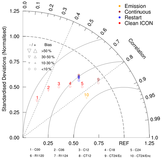
Figure 13 Taylor nomogram for modelled and observed daily PM_2.5 concentrations for all sensitivity experiments using different initial conditions and emissions. The red symbols indicate the clean initial simulations, the blue symbols represent the restart simulations, the brown symbols show the continuous simulation sensitivity experiment, and the orange symbols represent emission tests. The triangles and circles signify “Bias”. The triangle's size represents the bias value, and the direction of the triangle's vertex represents a positive or negative bias.

Table 4 Statistical measures of the modelled daily PM_2.5 in Xi'an (unit: µg m⁻³).

4.3 Model performance for SO₂ and NO₂

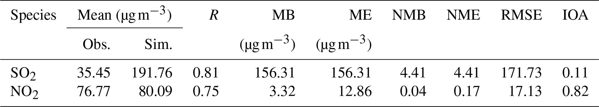
Sulfur dioxide (SO₂) and nitrogen dioxide (NO₂) concentrations are important precursors of SO₄ and NO₃, which are particulate matter components. Figure 14 shows the time series of daily average SO₂ and NO₂ concentrations from 13 NSAQ observation stations from the initial restart simulation, and the statistical results are listed in Table 5. The model shows an evident overestimation of SO₂, with an average bias of 156.31 µg m⁻³; the observed SO₂ concentration is also only 18 % of the simulated value. The main reason for this is the fact that the implementation of desulfurisation projects for important emission sources, such as coal-fired power plants, has not been fully considered, which has led to an overestimation of SO₂ emissions in the emission inventory. C. Li et al. (2017) found that the SO₂ emissions in China decreased by 75 % from 2007 to 2016 (i.e. SO₂ emissions in 2016 were about 25 % of those in 2007). In addition, the intensity of emission reduction has an uneven spatial distribution. The model performance of the NO₂ concentration is better: the IOA is 0.82, and the MB is only 3.32 µg m⁻³. There is high consistency in the variation trend between the simulated and observed SO₂ and NO₂ concentrations, with R values of 0.81 and 0.75 respectively.

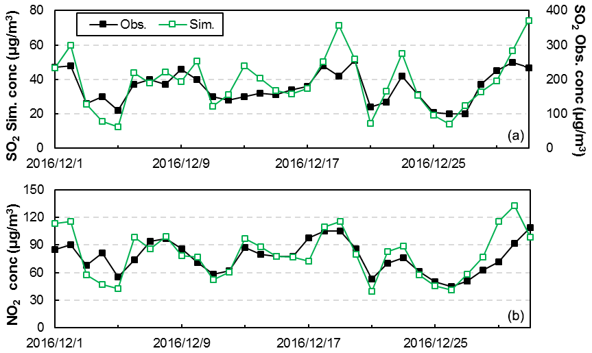
Figure 14 Time series of daily observed and simulated SO₂ (a) and NO₂ (b) concentrations averaged from 13 NSAQ observation stations during December 2016 in Xi'an. The black and green lines indicate observed and simulated results respectively.

Table 5 Statistical verification parameters of SO₂ and NO₂ during December 2016 in Xi'an. “Obs.” denotes observations, and “Sim.” denotes simulated values.

5 Conclusions

The WRF-SMOKE-CAMx model system was used to simulate fine particulate matter (PM_2.5) concentrations in Xi'an in December 2016. In this study, the construction fugitive dust emissions in Xi'an were added to the SMOKE model to update the local emission inventory. A series of model sensitivity experiments for the initial conditions and emissions were designed to improve the model performance in the Chinese megacity of Xi'an.

Three methods were applied for the initial condition tests: using the clean initial condition files as a clean initial simulation, using the restart files as a restart simulation, and a continuous simulation. The updated emission inventories drive all initial condition sensitivity experiments. The emission tests are based on the initial condition sensitivity experiment, which has the best model performance.

Comparing the model performance of PM_2.5 concentrations in different model sensitivity experiments in Xi'an, we found that the model combining the continuous simulation method and the updated local emission inventory can effectively improve the model performance. According to statistical parameters, for initial condition tests, the model performance is best for the CT24, C24, and R1120 and R1124 simulations. The R values range from 0.36 to 0.81 in all initial condition sensitivity experiments. The R value of CT24 is the largest and best in all initial condition sensitivity experiments. The R values of C24 and R1120/R1124 can reach 0.76 and 0.70 respectively. The MB values of CT24, C24, and R1120/R1124 are lower: 6.29, −3.72, and 4.01 µg m⁻³ respectively. The IOA of CT24, C24, and R1120/R1124 reached above 0.8: the IOA of CT24 was 0.9. Compared with other methods, the method of using the clean initial condition files has a longer simulation time and larger data volume. Therefore, the continuous simulation method for hindcasts, which is used to retrieve PM_2.5 concentrations, is suggested. For air quality forecasting, the restart simulation method is recommended. In addition, when simulating PM_2.5 concentrations using the CAMx model, the simulation requires a spin-up time of at least 27 h. This can improve the simulation results and reduce the simulation time.

This study updated the emissions inventory, which added construction fugitive dust emissions to the original emissions inventory. Compared with the simulation results based on the original emission inventory, the new simulation results, which were driven by the updated local emissions, showed much better performance with respect to PM_2.5 modelling. The absolute MB decreased from 35.16 to 6.29 µg m⁻³, and the IOA of simulation results with the updated local emissions was 0.90. Therefore, the right addition of emissions will also help to improve the simulation and forecasting.

Finally, we recommend the continuous simulation method for hindcasts, as it performs best for PM_2.5 concentrations and can also reduce the output of IO (daily grid instantaneous concentration) files to improve computing efficiency. For forecasting, the restart simulation method is suggested, which can reach similar model performance to the continuous simulation. If the restart simulation cannot be used owing to computing resource and storage space limitations when forecasting PM_2.5 concentrations, we attempt to extend the spin-up time as much as possible – to at least 27 h according to our results.

Appendix A: Statistical parameters for model evaluation

The mean bias (MB) was calculated as follows:

$$\begin{array}{}\text{(A1)}& \mathrm{MB}={\displaystyle \frac{\sum (M_i-O_i)}{n}}\end{array}$$

The mean error (ME) was calculated as follows:

$$\begin{array}{}\text{(A2)}& \mathrm{ME}={\displaystyle \frac{\sum \mathrm{|}{M}_i-O_i\mathrm{|}}{n}}\end{array}$$

The normalised mean bias (NMB) was calculated as follows:

$$\begin{array}{}\text{(A3)}& \mathrm{NMB}={\displaystyle \frac{\sum (M_i-O_i)}{\sum O_i}}\end{array}$$

The normalised mean error (NME) was calculated as follows:

$$\begin{array}{}\text{(A4)}& \mathrm{NME}={\displaystyle \frac{\sum \mathrm{|}{M}_i-O_i\mathrm{|}}{\sum O_i}}\end{array}$$

The root mean square error (RMSE) was calculated as follows:

$$\begin{array}{}\text{(A5)}& \mathrm{RMSE}={\left[{\displaystyle \frac{\mathrm{1}}{n}}\sum _{i=\mathrm{1}}^n{\left(M_i-O_i\right)}^{\mathrm{2}}\right]}^{\frac{\mathrm{1}}{\mathrm{2}}}\end{array}$$

The correlation coefficient (R) was calculated as follows:

$$\begin{array}{}\text{(A6)}& R={\displaystyle \frac{\sum _{i=\mathrm{1}}^n(M_i-\overline{M})(O_i-\overline{O})}{\sqrt{\sum _{i=\mathrm{1}}^n(M_i-\overline{M}{)}^{\mathrm{2}}\sum _{i=\mathrm{1}}^N(O_i-\overline{O}{)}^{\mathrm{2}}}}}\end{array}$$

The index of agreement (IOA) was calculated as follows:

$$\begin{array}{}\text{(A7)}& \mathrm{IOA}=\mathrm{1}-{\displaystyle \frac{\sum _{i=\mathrm{1}}^n(M_i-O_i{)}^{\mathrm{2}}}{\sum _{i=\mathrm{1}}^n(\left|M_i-\overline{O}\right|+\mathrm{|}{O}_i-\overline{O}\mathrm{|}{)}^{\mathrm{2}}}}\end{array}$$

The normalised standard deviation (NSD) was calculated as follows:

$$\begin{array}{}\text{(A8)}& \mathrm{NSD}={\displaystyle \frac{\sqrt{\frac{\sum _{i=\mathrm{1}}^n{\left(M_i-\overline{M}\right)}^{\mathrm{2}}}{n}}}{\sqrt{\frac{\sum _{i=\mathrm{1}}^n{\left(O_i-\overline{O}\right)}^{\mathrm{2}}}{n}}}}\end{array}$$

The normalised root mean square error (NRMSE) was calculated as follows:

$$\begin{array}{}\text{(A9)}& \text{NRMSE}=\sqrt{{\displaystyle \frac{\stackrel{\mathrm{‾}}{\left[\right(M_i-\stackrel{\mathrm{‾}}{M})-(O_i-\stackrel{\mathrm{‾}}{O}){]}^{\mathrm{2}}}}{{\mathit{\sigma }}_{O_i}}}},\end{array}$$

where M_i and O_i represent the simulated and observed value of a station respectively, n represents the number of stations, $\overline{M}$ and $\overline{O}$ represent the averages of the simulated and observed values respectively, and ${\mathit{\sigma }}_{O_i}$ represents the standard deviation over the observed value.