the Creative Commons Attribution 4.0 License.
the Creative Commons Attribution 4.0 License.
 | 23 Apr 2021
Ensemble prediction using a new dataset of ECMWF initial states – OpenEnsemble 1.0
Pirkka Ollinaho
Glenn D. Carver
Simon T. K. Lang
Lauri Tuppi
Madeleine Ekblom
Heikki Järvinen
Ensemble prediction is an indispensable tool in modern numerical weather prediction (NWP). Due to its complex data flow, global medium-range ensemble prediction has almost exclusively been carried out by operational weather agencies to date. Thus, it has been very hard for academia to contribute to this important branch of NWP research using realistic weather models. In order to open ensemble prediction research up to the wider research community, we have recreated all 50+1 operational IFS ensemble initial states for OpenIFS CY43R3. The dataset (OpenEnsemble 1.0) is available for use under a Creative Commons licence and is downloadable from an https server. The dataset covers 1 year (December 2016 to November 2017) twice daily. Downloads in three model resolutions (TL159, TL399, and TL639) are available to cover different research needs. An open-source workflow manager, called OpenEPS, is presented here and used to launch ensemble forecast experiments from the perturbed initial conditions. The deterministic and probabilistic forecast skill of OpenIFS (cycle 40R1) using this new set of initial states is comprehensively evaluated. In addition, we present a case study of Typhoon Damrey from year 2017 to illustrate the new potential of being able to run ensemble forecasts outside of major global weather forecasting centres.
- Article
(4803 KB) - Full-text XML
- BibTeX
- EndNote


The conventional method of predicting the future state of the atmosphere is to make a single-model forecast from the analysis which is the current best state estimate of the atmosphere. Due to limitations in observations and in the data assimilation system, an unknown amount of uncertainty remains in this state estimate. Moreover, the forecast model has its own uncertainties (see e.g. Leutbecher and Palmer, 2008). Ensemble forecast systems are designed to complement the deterministic forecast by providing a set of alternative but equally plausible future evolutions of the atmospheric state. The spread of these forecasts can be interpreted, for instance, in terms of the predictability of the current state, or as alternative forecasts.
For approximately the past 25 years, ensemble forecasting research has primarily been carried out by major operational forecasting centres or academic institutions closely collaborating with said centres. Without access to an ensemble prediction system (EPS), the majority of academic research on the topic has been limited to studying the end-products, i.e. various aspects of ready-made ensemble forecasts, or using idealized modelling set-ups. Although a great amount of progress has been made with respect to learning about and improving ensemble forecasts over the years, many open research questions and technical development possibilities still exist, for example (1) operational forecasting centres constantly reassess current operational implementations of initial state uncertainty (see e.g. Lang et al., 2015, 2019) and model uncertainty representations (see e.g. Lock et al., 2019) as well as exploring completely new methods (see e.g. Ollinaho et al., 2017; Leutbecher et al., 2017; Lang et al., 2021), (2) ensemble modelling studies of tropical storms (see e.g. Lang et al., 2012) offer a unique way to study forecast impacts of both initial state uncertainty and model uncertainty representations, and (3) EPSs provide a potent way of automating the model tuning process (Ollinaho et al., 2013, 2014; Tuppi et al., 2020).
This paper describes a new dataset of ensemble initial states covering a 1-year period twice a day, starting from 1 December 2016, courtesy of the European Centre for Medium-Range Weather Forecasts (ECMWF). The dataset, OpenEnsemble 1.0, is freely usable under a Creative Commons licence and can be downloaded from an https server (for the foreseeable future; see details in Sect. 4). Although the initial states are native to the OpenIFS model, there is no technical reason why they could not also be used to initialize any other forecasting model. However, implementing the initial states in such a fashion would likely not be a trivial task, and there would likely be a longer spin-up period affecting the forecast quality early on. We also present a workflow manager, called OpenEPS, to run OpenIFS ensembles from the new dataset. OpenEPS is also freely available under an Apache 2.0 licence.
We hope that the OpenEnsemble dataset and the workflow manager will enable the wider academic research community to contribute to ensemble forecasting research with realistic modelling tools. Additional new potential will also be made available to a variety of applications. For example, renewable energy production is dependent on weather conditions, such as cloudiness, wind speed, and icing. Increasing demand has clearly exposed this sector to the potential benefits of accurate weather forecasts. Utilizing ensemble forecasts in this context could reveal new sources of added value for users (see e.g. Sperati et al., 2016; Rasku et al., 2020). Ensemble forecasts are also important for flood-forecasting applications (Smith et al., 2016). Lastly, the available uncertainty information from ensemble forecasts has particular value for the prediction of extreme weather events, such as extra-tropical and tropical storms (see Friederichs et al., 2018, and references therein).
The dataset is aimed for use with the ECMWF OpenIFS model, which is described in Sect. 2. We discuss the initial state perturbation strategies used by ECMWF in Sect. 3. The dataset and instructions on how to use it are provided in Sect. 4. The OpenEPS software as well as a set-up for testing the dataset of initial states are described in Sect. 5. The performance of an OpenIFS ensemble started from the initial state perturbations is shown in Sect. 6.
The ECMWF Integrated Forecast System (IFS) was first used for operational forecasting in March 1994. Since that time, the IFS has been continually improved and its forecast performance has been assessed. The relative contribution of model improvements, the reduction in initial state error, and the increased use of observations to the IFS forecast performance is continuously monitored by ECMWF. Haiden et al. (2017) provides a detailed report on the IFS forecast performance for the IFS cycle 43R3, upon which the dataset described here is based. A detailed and up-to-date record of changes between IFS release cycles can be found in ECMWF (2019a).
The ECMWF OpenIFS activity, launched in 2011, provides a portable version of the IFS to ECMWF member state hydro-meteorological services, universities, and research institutes for research and education purposes for use on computer systems external to ECMWF. It is used in a wide range of studies, from teaching masters level courses to forecasting extreme events and inclusion in coupled climate models. As OpenIFS shares the same code base as IFS, the scientific forecast capability of the two models is identical, and the model description in this section applies equally to IFS except where indicated. The OpenIFS model supports all resolutions up to the ECMWF operational resolution and ensemble forecast capability. The ocean model, data assimilation, and observation handling components of IFS are not included in OpenIFS. A detailed scientific and technical description of IFS, applicable to OpenIFS, can be found in open access scientific manuals available from the ECMWF website (ECMWF, 2019b).
The OpenIFS model is a global model and uses a hydrostatic, spectral, semi-Lagrangian dynamical core for all forecast resolutions, with prognostic equations for the horizontal wind components (vorticity and divergence), temperature, water vapour, and surface pressure. The horizontal resolution is represented by both the spectral truncation wave number (the number of retained waves in spectral space) and the resolution of the associated Gaussian grid. Model resolutions are usually described using a Txxx notation, where xxx is the number of retained waves in spectral representation. An additional letter is used to describe the layout of the grid points used to compute, for example, the physical parameterization terms: TL is used to denote so-called 'linear' grids where the maximum wave number (shortest wave) is represented by the spacing between two adjoining grid points; TCO is used to denote the cubic-octahedral grid where the maximum wave number is represented by four grid points. Both of these grids use a reducing number of grid points along lines of latitude approaching the poles (see Malardel et al., 2016, for more details). OpenIFS based on IFS cycle 43R3 is the first with the capability of using the TCO horizontal grid. The vertical resolution varies smoothly with geometric height and is the finest in the planetary boundary layer, becoming more coarse towards the model top.
For a description of OpenIFS physical parameterizations, we refer the reader to the ECMWF online documentation (ECMWF, 2019b). OpenIFS contains the ECMWF wave model (ecWAM; ECMWF, 2019c). The IFS and OpenIFS models are normally run with ecWAM enabled to correctly represent the sea-state roughness and its impact on the lowest atmospheric layers, such as in momentum exchange. The OpenIFS model also includes stochastic parametrization schemes of IFS to represent model error (see Leutbecher et al., 2017, for an overview).
3.1 Singular vectors
Singular vectors (SV) represent the fastest-growing perturbations to a weather forecast – called the trajectory – within a finite time interval (Lorenz, 1965; Buizza, 1994; Palmer et al., 1998). In order to compute singular vectors, one linearizes the governing equations around a given trajectory. The idea behind using singular vector-based initial perturbations is that these are the dynamically most relevant structures and, hence, will dominate the forecast uncertainty (Ehrendorfer and Tribbia, 1997; Leutbecher and Palmer, 2008; Leutbecher and Lang, 2014). Here, growth is defined with respect to a specific metric. The metric used at ECMWF is the so called dry total energy norm (Leutbecher and Palmer, 2008), and singular vectors are computed with an optimization interval of 48 h and a spatial resolution of TL42 and 91 vertical levels. Different sets of singular vectors are computed: the leading 50 singular vectors for the Northern and Southern hemispheres and the leading 5 singular vectors for each active tropical cyclone (see Buizza, 1994; Puri et al., 2001; Barkmeijer et al., 2001; Leutbecher and Palmer, 2008, for details). While singular vectors targeted at the extra-tropics are optimized for the whole troposphere, singular vectors targeted at tropical cyclones are optimized for growth below 500 hPa.
3.2 Ensemble of data assimilations
At ECMWF, an ensemble of 4D-Var data assimilations (EDA, Buizza et al., 2008) is run to provide uncertainty estimates for both the ensemble forecasts and the high-resolution analysis. The EDA consists of a number of perturbed members and one unperturbed control member. Originally it was run with 10 perturbed members, but this changed in 2013 when the number of members was increased to 25. Recently the number of members was increased again to 50 (Lang et al., 2019). In this study, we make use of the EDA configuration with 25 perturbed members. For each EDA member the observations and sea surface temperatures are perturbed and the stochastically perturbed parameterization tendencies (SPPT) scheme is used to simulate the impact of model error.
3.3 Construction of initial perturbations
Perturbations based on the EDA short-range background forecasts are combined with singular vector-based perturbations to build the initial conditions for the ECMWF ensemble forecasts. EDA perturbations are derived by subtracting the mean of the EDA from each EDA member, resulting in a total of 25 perturbations. In addition to the EDA perturbations, 25 singular vector-based perturbations are generated.
Each of the 25 singular vector perturbations is constructed through a linear combination of the leading singular vectors which are calculated separately for the Northern Hemisphere (NH), the tropics (TR), and the Southern Hemisphere (SH). As such, each of the 25 singular vector perturbations contain some form of the calculated leading singular vectors in the NH/TR/SH. This is done by scaling the leading singular vectors by random numbers drawn from a multivariate Gaussian distribution (see Leutbecher and Palmer, 2008; Leutbecher and Lang, 2014).
The perturbations are centred on the high-resolution analysis and have a plus–minus symmetry, i.e. the initial conditions of the first perturbed ensemble forecast member are derived by adding the first EDA perturbation and the first singular vector perturbation to the high-resolution analysis. The initial conditions of the second perturbed ensemble forecast member are then obtained by subtracting the first EDA perturbation and the first singular vector perturbation from the high-resolution analysis, and so on. Thus, the initial perturbations of the even ensemble members have the opposite sign to the perturbations of the odd ensemble members. This set-up makes it possible to distribute the 25 EDA perturbations between the 50 ensemble forecast members. The plus–minus symmetry ensures that the mean of the perturbed analyses equals the unperturbed control analysis. Note that this is no longer the case from 2019 onwards in the operational ECMWF system. Following the introduction of the 50-member EDA the plus–minus symmetry is not required anymore (Lang et al., 2019).
Our dataset of ensemble initial states covers a 1-year period from 1 December 2016 to 30 November 2017. The initial states have been generated closely following what is done in the ECMWF operational ensemble. We use IFS cycle 43R3, which was operational from 11 July 2017 to 5 June 2018, to generate the ensemble initial states. This model version is also the basis for the OpenIFS release CY43R3v1. The single major difference to the operational ensemble set-up is that the highest model resolution available in OpenEnsemble is TL639 (∼ 32 km; instead of TCO639; ∼ 18 km). The other available resolutions provided in OpenEnsemble are TL399 (∼ 50 km) and TL159 (∼ 120 km).
The most relevant changes between this model version and the currently operational ECMWF version (CY46R1) that affect the ensemble initial states arise from changes to the model uncertainty representations (see Lock et al., 2019) and from the removal of the plus–minus symmetry. On top of this list, a number of changes have been introduced to the IFS model, the IFS data assimilation process, and the number of observations used in data assimilation. These all will naturally also affect the ensemble initial states, due to direct or indirect contributions.
Table 1Description of the OpenIFS and ecWAM initialization files.

In order to run the OpenIFS forecast model, multiple initialization files are needed, and these are listed in Table 1 along with an explanation of the function of the file. The initialization beginning with “ICM” are the initial files for the upper-air variables, surface variables, and climatological forcing in the atmospheric part of the model. The four dots (....) in these files are replaced by a four-letter experiment identifier of your own choosing. In the OpenEnsemble files this identifier is “oifs”. The ICMGG....INIUA files contain upper-air model-level variables on a Gaussian grid. ICMSH....INIT files contain model-level variables in spherical harmonics representation. ICMGG....INIT files contain surface-level variables on a Gaussian grid. The ICMCL....INIT files contain climatological surface fields for albedo at different radiation wave lengths, leaf area indexes, soil temperature, and sea ice area fraction. For a detailed description of the contents of each file, we refer the reader to Appendix A. In addition to these four date-specific files, OpenIFS requires static climatological files for radiation calculations and text Fortran namelists defining the supported grid resolutions for the radiation scheme and the vertical hybrid sigma coordinates. In order to utilize ecWAM, a separate set of wave model input files and namelists is required. The OpenEnsemble dataset contains files 1–4, and an example of file 5 is also provided. Files 6–8 can be obtained from the ECMWF anonymous ftp server (ftp://ftp.ecmwf.int/pub/openifs/ifsdata/, last access: 11 March 2021). The additional files needed to enable ecWAM are also provided in OpenEnsemble 1.0 (files 9–15).
The OpenIFS date-specific data (files 1–4) are tarred, gzipped, and packed such that a single tarz file contains all initial states (control state and perturbed initial states) for a given date and time (00:00 and 12:00 UTC). The files are in the following form: “YYYYMMDDHH.tarz”. Furthermore, the data are arranged into separate directories for the three available resolutions:
-
https://a3s.fi/oifs-t159/YYYYMMDDHH.tgz (last access: 11 March 2021) (∼ 1.4 GB per file);
-
https://a3s.fi/oifs-t399/YYYYMMDDHH.tgz (last access: 11 March 2021) (∼ 7.9 GB per file);
-
https://a3s.fi/oifs-t639/YYYYMMDDHH.tgz (last access: 11 March 2021) (∼ 19.5 GB per file).
Additionally, example OpenIFS namelists for CY43R3 and the ecWAM common and date-specific files can be downloaded from
-
https://a3s.fi/oifs-tRES/fort.4_namelist_example (last access: 11 March 2021),
-
https://a3s.fi/wam/oifs_cy43r3_tRES_wam_common.tgz(last access: 11 March 2021),
-
https://a3s.fi/wam/oifs_cy43r3_tRES_wam_inifiles_YYYYMM.tgz (last access: 11 March 2021).
Here, RES is replaced by the required resolution (), and YYYYMM is replaced by year and month. Note that the ecWAM date-specific files (6) are packed into month-long tarz files.
Table 2 lists the types of files a single OpenIFS date-specific tarz file consists of. In each tarz file there are a set of 50 different perturbation files as well files 1–4 listed in Table 1 for running an unperturbed control experiment. The perturbation files follow the IFS naming convention: (1) pan – perturbed analysis (EDA perturbations), (2) psu – perturbed surface (EDA perturbations), (3) pua – perturbed upper air (UA) file (EDA+SV perturbations), and (4) pert – raw SV perturbations.
Table 2Files contained in a tarz file for a given date and time. RES is replaced with the spherical truncation number, i.e. .
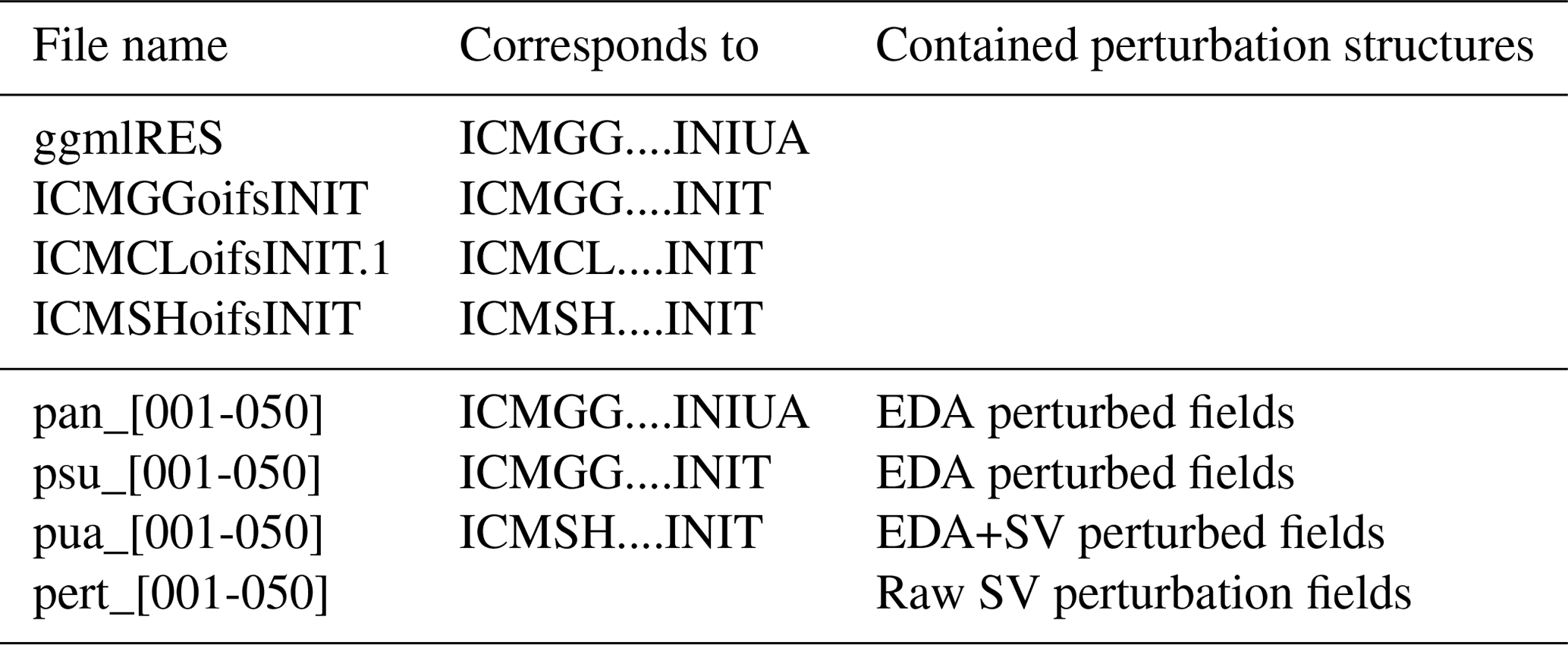
Table 3Types of initial states that can be constructed from the dataset.
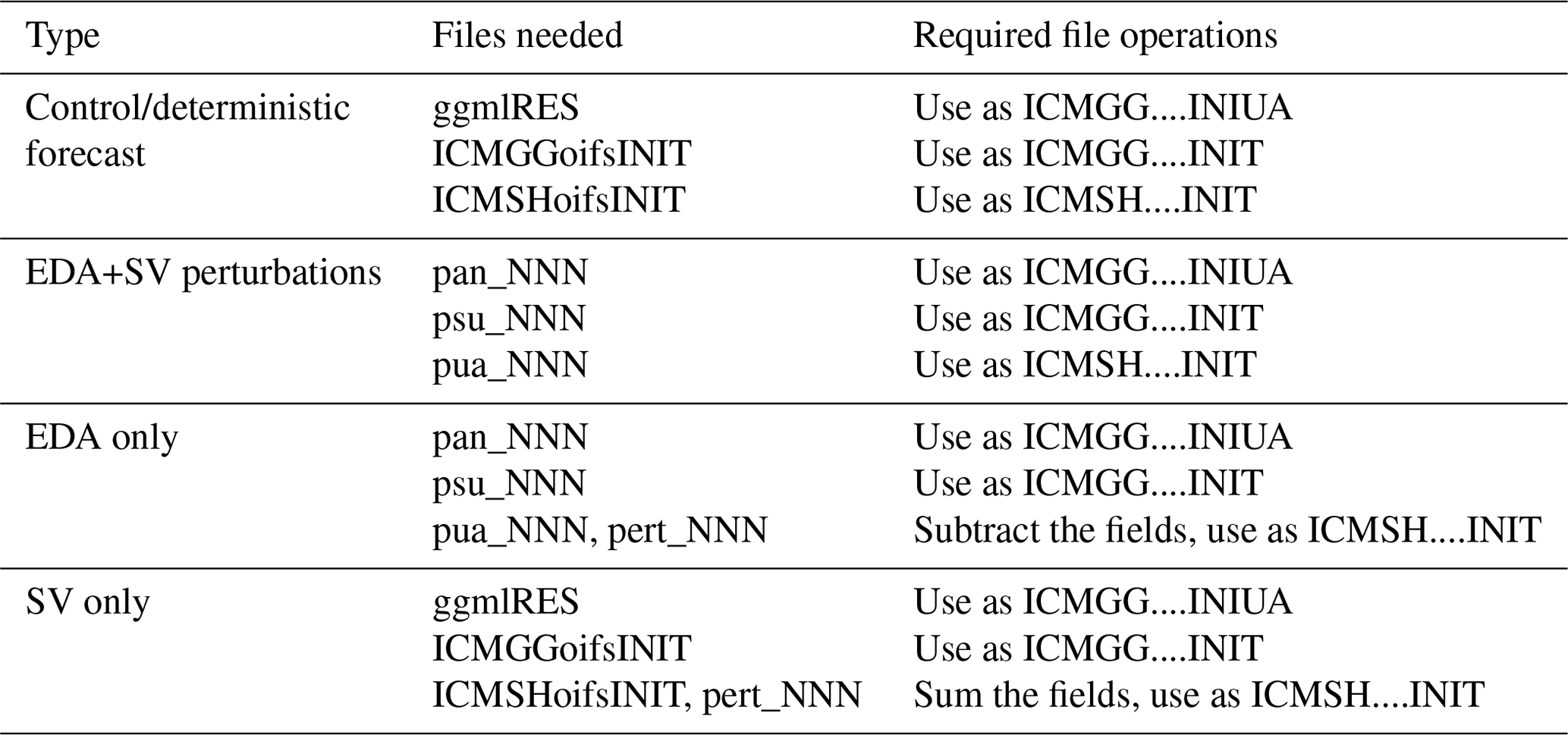
The last four files in Table 2 contain different forms of initial state perturbations. pan_NNN files can be used to replace ICMGG....INIUA and are constructed as high-resolution analysis ± EDA perturbations. psu_NNN files can be used to replace ICMGG....INIT files and contain initial states with EDA perturbations. pua_NNN files can be used to replace ICMSH....INIT and contain the final spherical harmonics representation of an initial state containing both EDA and SV perturbations. And finally, pert_NNN files contain raw SV perturbations in spherical harmonics. These can be used to decompose the ICMSH....INIT file into SV and EDA parts.
These files can be used to form four different kinds of initial states for experimentations, which are listed in Table 3. Control forecasts and SV+EDA perturbed forecasts can be initialized directly from the provided files. For EDA-only or SV-only perturbations, some file operations are required. In order to get initial states with EDA-only perturbations, the pert file needs to be subtracted from the pua file. An example of how to do this using Climate Data Operators (CDO; Schulzweida, 2019) software is given in Appendix B. The file manipulation is always subtraction: the plus–minus symmetry is built into the files, i.e. pert_001 and pert_002 will be identical fields with different signs. For SV-only perturbations, the control state should be used, and the pert files should be added to the ICMSH....INIT files. Again, the same procedure with grid point conversion and plus–minus symmetry applies here. The workflow shown in Appendix B can be applied here with minor modifications. Note that OpenIFS expects to find the files 1–4 listed in Table 1, so the initial files must be renamed or linked accordingly when running forecasts.
When using ecWAM with OpenIFS (the recommended configuration), the ecWAM date-specific files (9–12 in Table 1) and ecWAM common files (13–15 in Table 1) should be linked to the forecast run folder as well.
5.1 Workflow manager – OpenEPS
In order to run large ensembles of a forecast model, a workflow manager is essential. For this purpose, we use a simple yet efficient software called OpenEPS here. We want to emphasize that the dataset of initial states provided is not tied to this (or any) software. OpenEPS is mostly written in Bash but utilizes GNU Make to handle parallel job executions in high-performance computing (HPC), Linux cluster, or laptop environments. The software is freely available under an Apache 2.0 licence (https://github.com/pirkkao/OpenEPS, last access: 12 March 2021). Instructions on how to use the software, as well as a few example cases, are provided with the software download. Nonetheless, we will provide a concise description of the OpenEPS software here, as the workflow would be similar with any workflow manager. The general workflow is handled as follows:
- 0.
set up a computing-environment-specific file containing various architecture settings;
- 1.
choose the experiment specifications (resolution, number of ensemble members, computing resources, etc.);
- 2.
run OpenEPS, which will
- –
construct the required path structure for the experiment,
- –
generate run configurations (fort.4) for OpenIFS,
- –
link the full initial states or generate a set of initial states from the dataset (SV only, EDA only, or change amplitudes of the perturbations) for the first ensemble initialization date,
- –
reserve run resources for the model execution and submit the batch job (if run on an HPC);
- –
- 3.
run OpenIFS model forecasts for the given date with the available resources;
- 4.
once all ensemble member forecasts are complete, execute one or more of the following
- –
post-process model outputs,
- –
run additional tasks e.g. algorithmic model tuning;
- –
- 5.
link or generate initial states for the next date;
- 6.
go back to step 3 until all dates have been cycled through.
Step 0 only needs to be completed once for each unique computing environment. In the current HPC implementation, OpenEPS reserves all of the desired computing resources at the same time. For example, if the user wanted to run a total of five ensemble members, each to be executed concurrently and each using 20 cores, this would mean submitting a batch job requesting a reservation of 100 cores for a time slot of N minutes. If the user wanted to run 50 ensemble members in total following the previous set-up, OpenEPS would compute these in 10 consecutive batches within the same batch reservation. Instead of reserving 100 cores for N minutes, the cores would now be reserved for N⋅10 min. One could also naturally increase the amount of computing resources in order to keep the execution time to a minimum, i.e. reserve 100⋅10 cores for N minutes.
It is also possible to do online post-processing within the workflow, i.e. run scripts to manipulate each model forecast after they are finished. Note that, due to the nature of the HPC implementation, this means that all of the reserved resources might be sitting idle while this is happening. Usually the computing resources required for model forecast calculations are much larger than those used in post-processing the output, so caution is advised here. We recommend using this option only when online post-processing is required as part of the workflow, such as in algorithmic model tuning. Also, as manipulation of the initial state files is resource demanding, it is highly advisable that modifications to the initial states (separation of SV and EDA parts for example) are done as a separate task before the actual model integrations. The workflow for this is also supported in OpenEPS.
5.2 Forecast model set-up
Although the initial states have been generated using IFS version CY43R3, we use the OpenIFS version matching IFS CY40R1 as the forecast model here. This is due to practical reasons: at the time of writing this paper, the matching cycle for OpenIFS (CY43R3v1) was still in preparation. We foresee that the forecast model difference will affect the testing somewhat, mainly due to differing analysis and forecast biases, i.e. the analysis bias is affected by the model cycle; hence, a CY43R3 analysis and CY43R3 forecast model will have more similar biases than a CY43R3 analysis and a CY40R1 forecast model. This will result in potentially better scores when the analysis and forecast are created by the same cycle. The forecasting skill in early forecast lead times might also be somewhat degraded due to a stronger than usual spin-up effect. However, we still feel confident that the forecast skill evaluation is of value despite the forecast model differences. A number of physical parametrization and model dynamics changes happened between CY40R1 and CY43R3; we refer interested readers to the ECMWF OpenIFS and IFS websites (ECMWF, 2020a, 2019a, b).
5.3 Experiment set-up
We have run a number of experiments in order to assess how well the initial state perturbations fare with OpenIFS; these are listed in Table 4. The experiments cover the three horizontal resolutions provided: TL159 (∼120 km), TL399 (∼50 km), and TL639 (∼32 km). Also, the different initial perturbation types (SV and EDA) were tested separately and together in order to illustrate the efficiencies of the perturbations in generating ensemble spread with the OpenIFS set-up. All of the experiments were run without any model uncertainty representations. We want to note that the decision to include the ecWAM initial states in this release version of the OpenEnsemble dataset came during the review process. Therefore, the experiments shown here were run without ecWAM activated.
Table 4Experiments conducted for this study. The experiment name includes the resolution used as well as the type of initial state perturbations (pert) used. The ensemble sizes, the number of ensemble initialization dates, and notes regarding the specific experiments are also given.
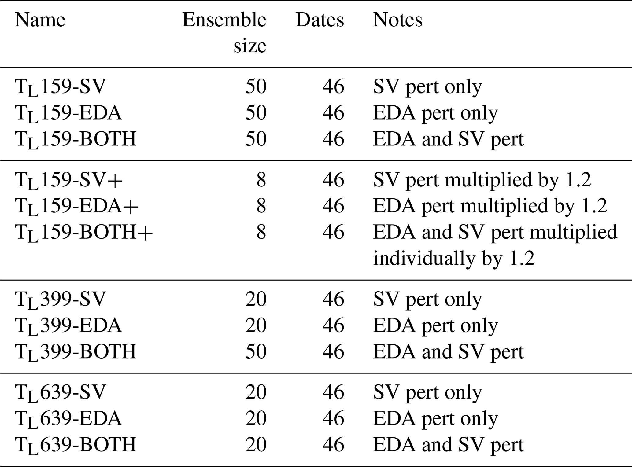
Running large numbers of ensemble forecasts requires substantial computational resources. Leutbecher (2019) demonstrated that the number of ensemble start dates is much more important than the size of the ensemble for extracting the mean probabilistic skill of the system. Thus, we keep the number of start dates high but decrease the ensemble size for the higher resolutions in order to save computational resources: only the TL159 experiments and the basic set-up for TL399 were run with the full 50 ensemble members. TL399 experiments testing the effect of the initial state perturbation methods individually were run with a reduced ensemble size of 20 members as were all of the TL639 experiments. Using fair scores, we will showcase (in Sect. 6.2) that the ensemble size chosen here is indeed more than enough to extract the probabilistic skill of the system.
An additional set of experiments with TL159 resolution was also run in which the amplitudes of SV and EDA perturbations were inflated by multiplying the perturbation fields with a constant number. This exercise aimed to demonstrate how the initial state amplitudes can be used to tune the ensemble skill. In the combined perturbations experiment (BOTH+), both of the perturbation types were increased individually and then added together. These experiments used an ensemble size of eight members.
6.1 Ensemble mean RMSE and ensemble spread
It is common to assess the skill of an ensemble by calculating the ensemble mean root-mean-squared error (RMSE) and the ensemble standard deviation (ensemble spread). The former measures how accurate the ensemble mean is, i.e. how near the mean of the ensemble forecasts is to analysis fields or observations; the latter verifies whether the ensemble forecasts simulated a wide enough range of possible atmospheric states to reflect the error characteristics of the ensemble mean. Ideally, one would want the ensemble mean RMSE to be as small as possible and the spread to be equal to the ensemble mean RMSE on average over many cases and within sampling uncertainty caused by a finite number of cases and ensemble members (see Leutbecher and Palmer, 2008, for an in-depth discussion). Here, we use operational ECMWF analyses truncated to a regular grid from the forecast period as the truth. The operational analyses are available at a 6-hourly interval instead of the 12-hourly interval available through OpenEnsemble 1.0. We want to note that the operational ECMWF analyses covering the same time period as OpenEnsemble 1.0 use two different IFS versions: CY43r1 is used until 10 July 2017 and CY43r3 is used from 11 July onwards. Thus, even when using OpenIFS version CY43r3 to generate forecasts from OpenEnsemble 1.0, verification scores calculated with operational ECMWF analyses might appear somewhat degraded due to differences in the underlying model version. The model output is interpolated to a regular grid before any other post-processing is done.
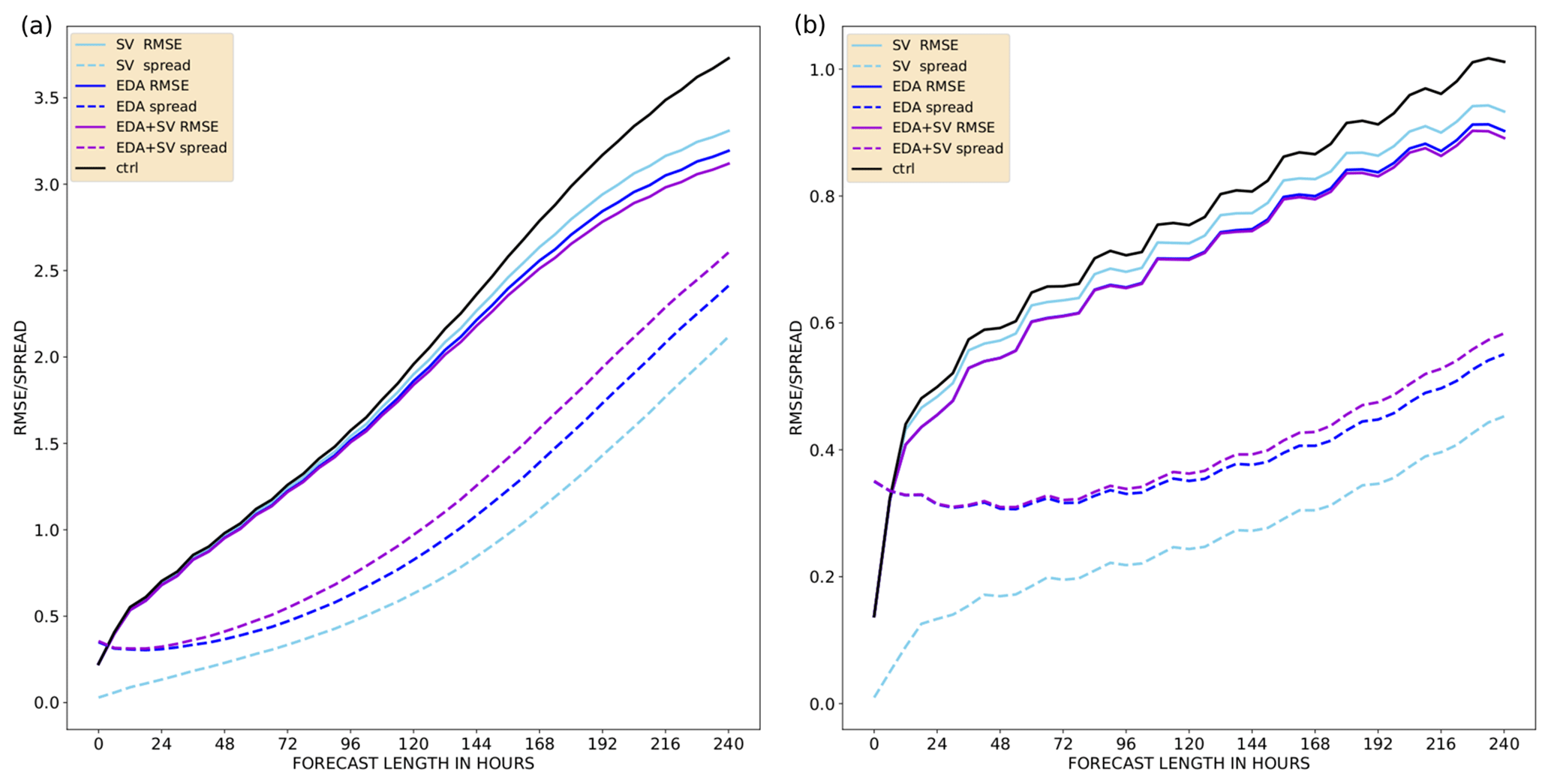
Figure 1Ensemble mean RMSE (solid) and ensemble spread (dashed) of temperature at 850 hPa as a function of forecast lead time up to 240 h for a TL159 model resolution with 50 ensemble members. The mean is calculated over 46 start dates. The experiments included are as follows: only SV perturbations (cyan), only EDA perturbations (blue), and both SV and EDA perturbations (violet). Also shown here is the unperturbed control member RMSE (black). Panel (a) shows the Northern Hemisphere, and panel (b) shows the tropics.
In Fig. 1, the ensemble mean RMSE (solid) and ensemble spread (dashed) are shown for the first three TL159 experiments (SV, EDA, and BOTH). Figure 1a represents scores for the Northern Hemisphere (NH), and Fig. 1b represents scores for the tropics (TR). The EDA perturbations produce more ensemble spread than the SV perturbations in both the NH and TR. It is also quite evident that including both of the perturbations further improves the ensemble spread, i.e. it moves closer to the ensemble mean RMSE. Both kinds of perturbations also improve the forecast skill of the system when compared with a control run without any perturbations (black line). Interestingly, the EDA perturbations do not really start to grow before a forecast length of 48 h in the NH and 96 h in the TR. The added benefit of having both of the perturbation types active at the same time can also be observed in the mean forecast skill beyond forecast lead times of 5 (8) d in the NH (TR). The behaviour with respect to the types of initial state perturbations is similar at resolutions of TL399 and TL639 (not shown).
An increased horizontal resolution leads to a much improved system forecast skill, as can be seen in Fig. 2 where the experiments with both SV and EDA perturbations active are plotted for all three resolutions. For both TL399 and TL639 resolutions, this is due to both a larger spread and an improved forecast skill of the ensemble. Note that there is a sampling difference between the two lower-resolution experiments and the TL639 experiment: the former two cases have 50 ensemble members, whereas the latter case has 20. Ideally, one should account for the finite number of members when comparing ensemble spread and error (see Leutbecher and Palmer, 2008).
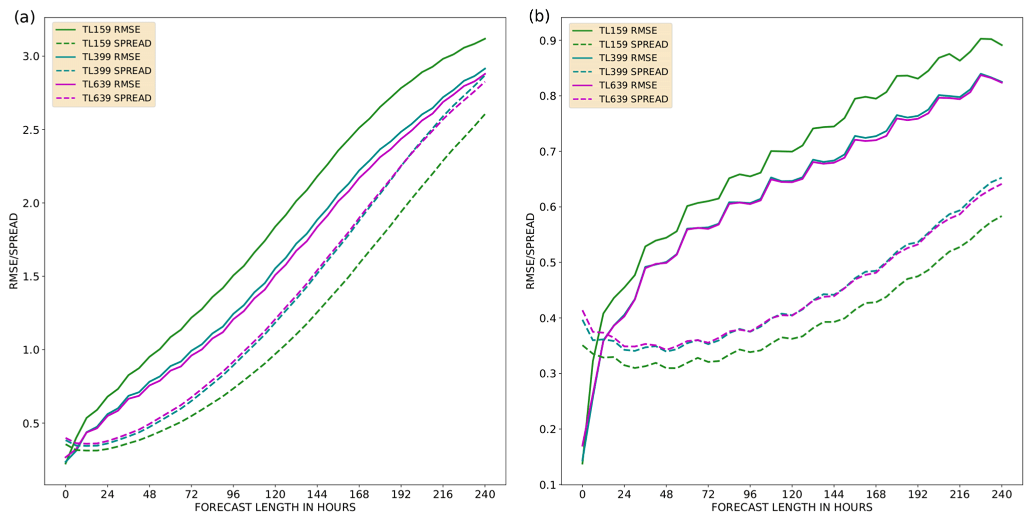
Figure 2Ensemble mean RMSE (solid) and ensemble spread (dashed) of temperature at 850 hPa as a function of forecast lead time up to 240 h. The mean is calculated over 46 start dates. All experiments contain SV and EDA perturbations: TL159 (green; 50 members), TL399 (teal; 50 members), and TL639 (violet; 20 members). Panel (a) shows the Northern Hemisphere, and panel (b) shows the tropics.
6.2 Fair continuous ranked probability score (CRPS)
Fair versions of probabilistic skill scores indicate how the system would have scored if it had had an infinite number of ensemble members1. Leutbecher (2019) illustrated how a fair version of the continuous ranked probability score (CRPS) can be constructed and also explored how many ensemble members are required to calculate a representative fair CRPS. The recommended ensemble size was set to be four to eight members for scientific testing. Figure 3a shows the regular CRPS calculated for ensembles of various sizes. Figure 3b shows the fair CRPS values for the same experiments. The smaller ensembles are constructed from the 50-member ensemble. A mathematical prerequisite for calculating the fair CRPS is that the ensemble members need to be exchangeable, which is not fulfilled in the ECMWF ensemble under this initial state construction style, where the SV and EDA perturbations are used with plus–minus symmetry (see Leutbecher, 2019). Note that this is no longer the case from 2019 onwards in the ECMWF operational ensemble configuration. Therefore, the smaller ensembles here are either constructed from odd or even ensemble members, which fulfils the prerequisite. As per construction, the regular CRPS is lower (i.e. better) for an ensemble with more members than for an ensemble with fewer members (Fig. 3). But, the fair version of the score gives near-identical results for the different ensemble sizes. This allows us to meaningfully compare different configurations.
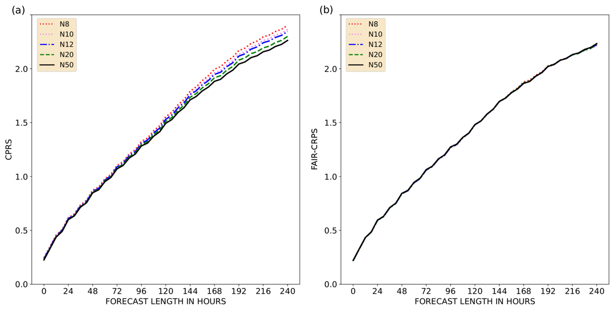
Figure 3CPRS (a) and fair CRPS (b) of temperature at 850 hPa as a function of forecast lead time, up to 240 h. The mean is calculated over 46 start dates. Both panels show the TL159-resolution scores for the Northern Hemisphere, with different colours and line styles representing the various ensemble sizes used to calculate the scores: 50 (continuous black), 20 (dashed green), 12 (dot-dashed blue), 10 (dotted pink), and 8 (dotted red).
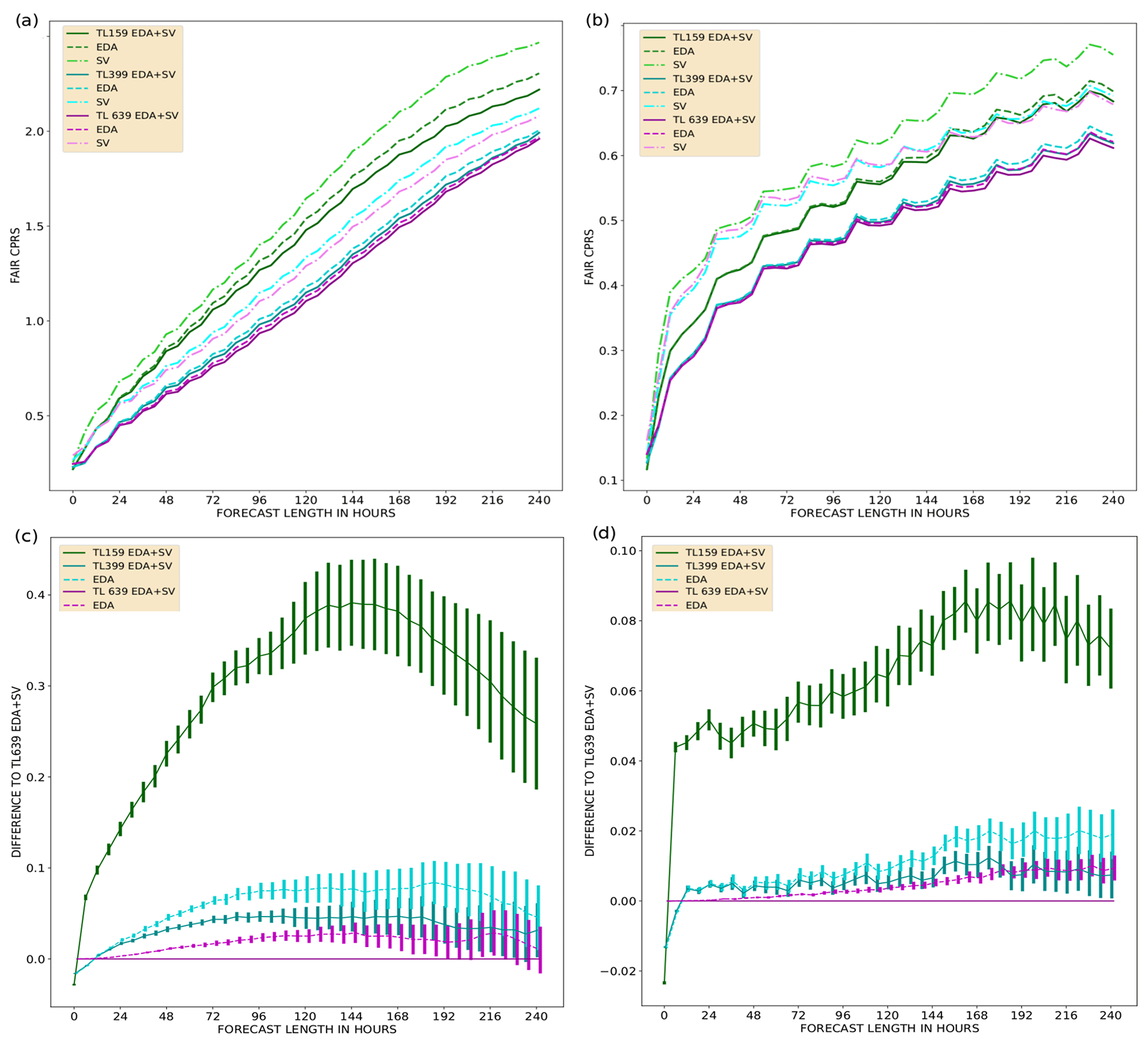
Figure 4Fair CRPS as a function of forecast lead time, up to 240 h, for the Northern Hemisphere (a) and the tropics (b). The mean is calculated over 46 start dates. Fair CRPS difference to the TL639 EDA+SV experiment with 95 % confidence intervals for the Northern Hemisphere (c) and the tropics (d). Scores for eight-member ensembles with various resolutions and perturbation methods: TL159 (green), TL399 (cyan), TL639 (violet), SV perturbations only (dot-dashed), EDA perturbations only (dashed), and both SV and EDA perturbations (solid).
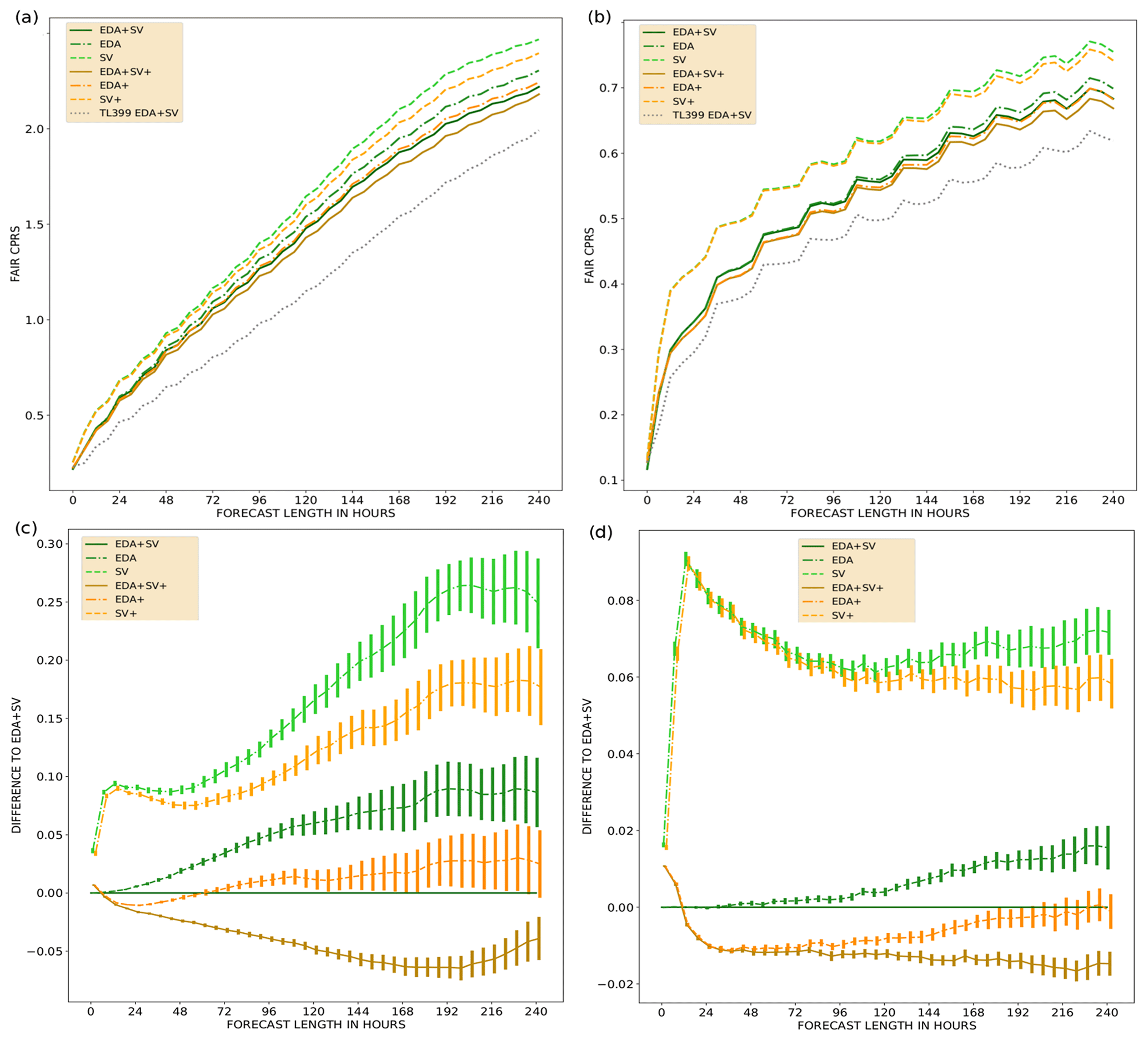
Figure 5Fair CRPS as a function of forecast lead time, up to 240 h, for the Northern Hemisphere (a) and the tropics (b). The mean is calculated over 46 start dates. Fair CRPS difference to EDA+SV experiment with 95% confidence intervals for the Northern Hemisphere (c) and the tropics (d). Scores for eight-member ensembles with a TL159 resolution using various perturbation methods: SV perturbations only (dashed), EDA perturbations only (dot-dashed), and both SV and EDA perturbations (solid). Normal amplitude initial state perturbations (green) and initial state perturbations increased by a factor of 1.2 (orange/brown). The TL399 experiment with both SV and EDA perturbations (black dashed) is drawn for reference (a, b).
Figure 4a and b show fair CRPS for all of the experiments using standard initial state perturbation amplitudes. Additionally, Fig. 4c and d show pairwise fair CRPS differences with 95 % confidence intervals (calculated via bootstrapping) between the TL639 EDA+SV experiment and selected experiments. Using only SV perturbations results in less skilful ensembles than using only EDA perturbations; this is in line with the findings of Buizza et al. (2008) and Lang et al. (2012). Noticeably, a TL159 resolution with EDA perturbations scores better in the tropics than TL639 with only SV perturbations active for forecast lead times shorter than about 168 h. The SV perturbations in the tropics only consist of perturbations around active tropical cyclones; thus, it is expected that the SV perturbations will result in a higher fair CRPS than the EDA perturbations in the tropics. Nonetheless, having SV perturbations active on top of EDA perturbations brings clear value to all the resolutions in both the NH and TR. Interestingly, when comparing the EDA+SV experiments for the different resolutions, TL159 scores the best whereas TL639 scores the worst for the 0th time step of the model integration. This is likely caused by analysis and forecast model version differences.
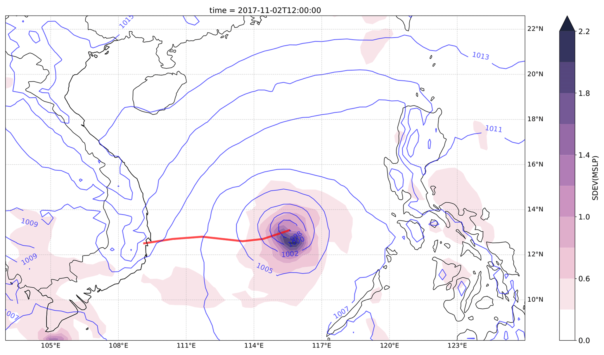
Figure 6Ensemble mean sea level pressure (MSLP; violet contour lines) and ensemble spread (coloured contours) at a TL639 resolution. The 0 h forecast was initialized on 2 November at 12:00 UTC. The observed track of Typhoon Damrey between 2 November at 12:00 UTC and 4 November at 00:00 UTC (red line).
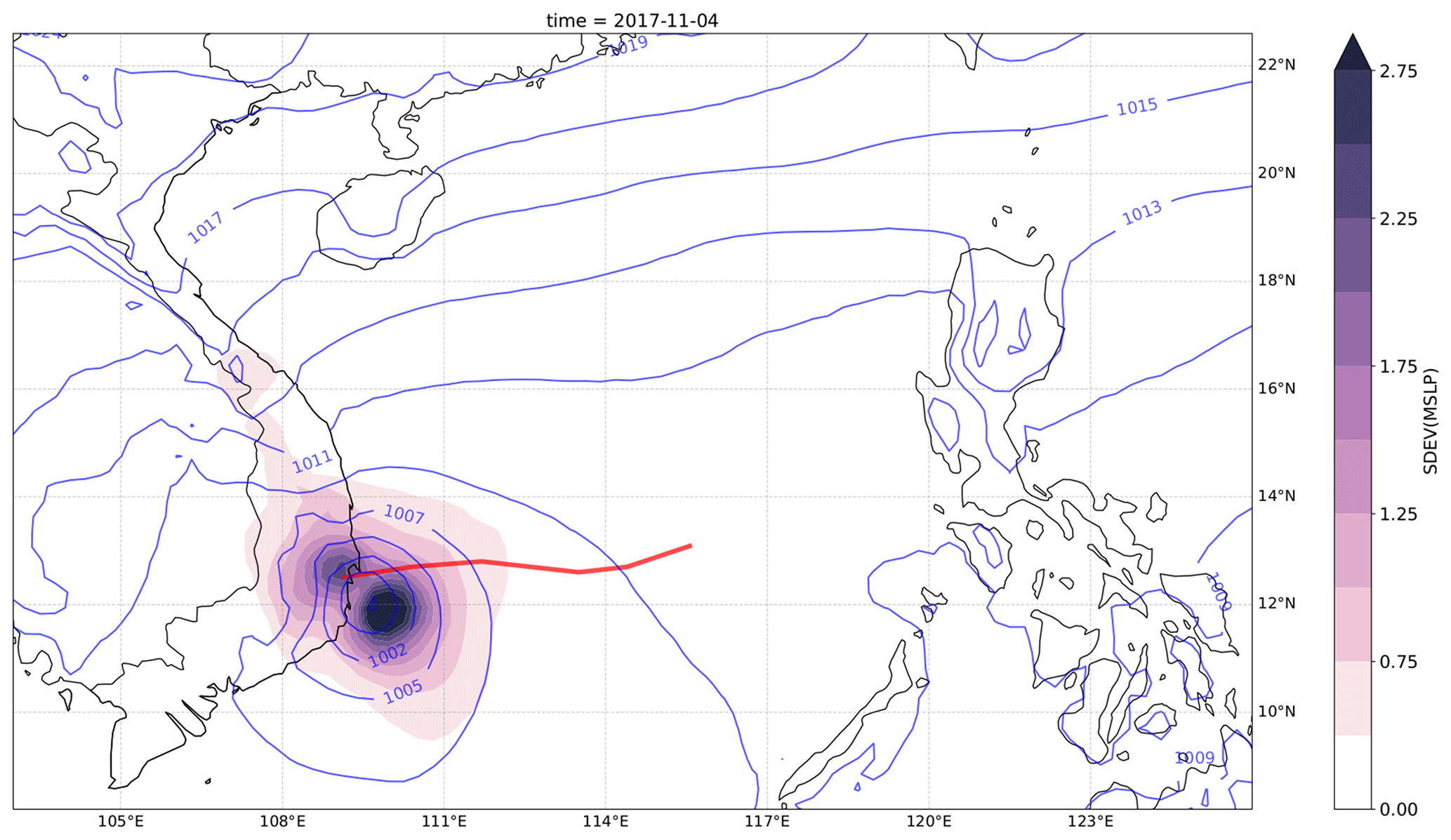
Figure 7Ensemble mean MSLP (violet contour lines) and ensemble spread (coloured contours) at a TL639 resolution. The 36 h forecast was initialized on 2 November at 12:00 UTC. The observed track of Typhoon Damrey between 2 November at 12:00 UTC and 4 November at 00:00 UTC (red line).
The SV perturbation amplitude is a tuning parameter of the ensemble (Leutbecher and Palmer, 2008; Leutbecher and Lang, 2014). Figure 5 illustrates the sensitivity of the TL159-resolution ensemble to a change in the initial perturbation amplitude. There is a noticeable increase in skill beyond a 12 h forecast lead time in the NH when increasing the EDA perturbation amplitudes by a factor of 1.2. Increasing the SV perturbation amplitudes results in an increase in skill for all forecast lead times. In the TR, the increase in skill becomes noticeable beyond a forecast lead time of 12 h (48 h) for EDA (SV) perturbations.
We have focused on showing the forecast skill of temperature at 850 hPa over the NH and the TR. The results from other model variables (geopotential at 500 hPa, winds at 200 and 850 hPa) show very similar behaviour (not shown). Moreover, the Southern Hemisphere forecast skill is very much like that in the NH (not shown).
The following case study is aimed at illustrating the usefulness of the new dataset and the OpenEPS repository. We want to emphasize that the goal here is not to dissect how the ensemble behaved or what caused the differences in the forecasts, but to give an idea of how running ensembles can provide plenty of insights that are normally unavailable from a single-model forecast.
Typhoon Damrey started as a tropical depression in the Philippine archipelago on 31 October 2017. After moving across the open sea to the west of the Philippines, it started to rapidly intensify and reached its peak strength on 3 November (the control forecast initial state for MSLP and 200 hPa wind vectors for 2 November at 12:00 UTC is illustrated in Appendix C Fig. C1). The typhoon made a landfall in Vietnam the following day and caused severe damage and loss of life (see e.g. GFDRR, 2018). A report on the operational forecasting performance of the event can be found in the ECMWF Severe Event Catalogue (ECMWF, 2020b).
We use our dataset to launch a 20-member OpenIFS ensemble starting from 2 November at 12:00 UTC with both SV and EDA perturbations active and a TL639 resolution. The ensemble mean MSLP and ensemble spread for the 0th time step of the ensemble forecast is shown in Fig. 6. The observed track of Typhoon Damrey is also plotted (red). Notably, the largest differences in the initial states are focused on the southern side of the typhoon core (MSLP minimum). Large differences can also be observed in the east–west structure of the typhoon. Lang et al. (2012) showed how especially the SV perturbations can rapidly alter the location and intensity of a tropical cyclone (TC). Model forecast differences (due to the initial state perturbations) after a 36 h forecast lead time are shown in Fig. 7. The ensemble mean as well as the majority of the ensemble members place the landfall location too far south and propagate the typhoon core too slowly (too far east). The exact location and timing of the typhoon landfall are, however, within the likely solutions from the ensemble.
These kind of case studies using ensembles could be used to study various mechanics of the model and answer the following questions:
-
Was there already something incorrect in the TC structure in the unperturbed initial state?
-
Did some initial state perturbations correct this and make an impact on the TC forecast?
-
Were local perturbations to the typhoon core essential or was it perhaps more important to get the mean flow forcing right?
-
Would activation of the OpenIFS wave model improve all of the forecasts due to an improved representation of momentum exchange between the ocean surface and the atmosphere?
In this paper, we have introduced a dataset of ensemble initial states covering a 1-year period from 1 December 2016 to 30 November 2017. The initial states have been generated closely following what is done operationally in the ECMWF ensemble and are based on ECMWF IFS cycle 43R3. Three horizontal resolutions are provided for 50+1 ensemble members: TL159 (∼120 km), TL399 (∼50 km), and TL639 (∼32 km). The provided files can be used to construct three types of initial states: (1) both SV and EDA perturbations (as in the operational ECMWF ensemble), (2) SV-only perturbations, and (3) EDA-only perturbations. The dataset is available for download from an https server under a Creative Commons licence.
In order to showcase the average forecast skill of the dataset, we ran forecast experiments covering all three horizontal resolutions and all three different initial perturbation types. The experiments were run with OpenIFS CY40R1 (the newest OpenIFS version available at the time of writing). We used an open-source workflow manager, called OpenEPS, to manage the ensemble workflow on an HPC.
For all resolutions, SV perturbations generate the least spread in the ensemble. Nonetheless, having SV perturbations active on top of EDA perturbations clearly brings value to the forecast skill of the system. All perturbation types increase the accuracy of the ensemble mean when compared against a control forecast initialized from an unperturbed analysis state. We have also tested the impact of inflating the amplitudes of the initial state perturbations. Increasing the amplitudes of the initial state perturbations result in an increase in the forecast skill of the system, demonstrating that inflation tuning of the initial conditions can improve probabilistic skill. Activating ecWAM when running OpenIFS degrades some skill scores in the TR (not shown). This is a known issue in IFS and has been fixed gradually over the newer operational IFS cycles (Jean Bidlot, personal communication, 2021). Despite the unfavourable effect on the skill of some variables in the TR, we highly recommend running OpenIFS with ecWAM activated, as including the wave model is known to especially improve forecasts of extra-tropical and tropical cyclones.
Inspection of especially the lowest-resolution experiments reveals that all of the ensembles are under-dispersive, i.e. the ensemble spread is much smaller than the ensemble mean RMSE. Also, the EDA perturbations in the tropics do not grow during the first 96 h of the forecasts. This is expected as our ensemble configuration is missing a model uncertainty representation. In operational ensemble configurations, having one or more model uncertainty representations has been essential in both improving the accuracy of the ensemble mean as well as increasing the spread of the ensemble. Assessing the ensemble skill when one or multiple model uncertainty representations are active on top of the initial state perturbations is something that the authors will proceed to work on next. The OpenIFS release based on IFS CY43R3 includes the stochastically perturbed parameterization tendencies (SPPT) scheme (Buizza et al., 2008), the stochastic kinetic energy backscatter (SKEB) scheme (Berner et al., 2009), and an early version of the stochastically perturbed parametrizations (SPP) scheme (Ollinaho et al., 2017). To assess the skill of ensemble forecasts, it is also important to take biases, analysis uncertainty, and observation errors into account (Yamaguchi et al., 2016). This is something that we plan to do in the future.
We have also briefly demonstrated the potential of using ensemble forecasts in case studies. Typhoon Damrey, which caused severe damage in Vietnam in 2017, was simulated by generating a 20-member ensemble with a TL639 resolution initialized from our dataset of initial state perturbations.
We hope that the meteorological research community will find this dataset and the OpenEPS repository useful in striving towards more realistic experimentation in ensemble forecasting.
Table A1Surface-level variables on a Gaussian reduced grid in the ICMGGoifsINIT file. WMO stands for World Meteorological Organization.
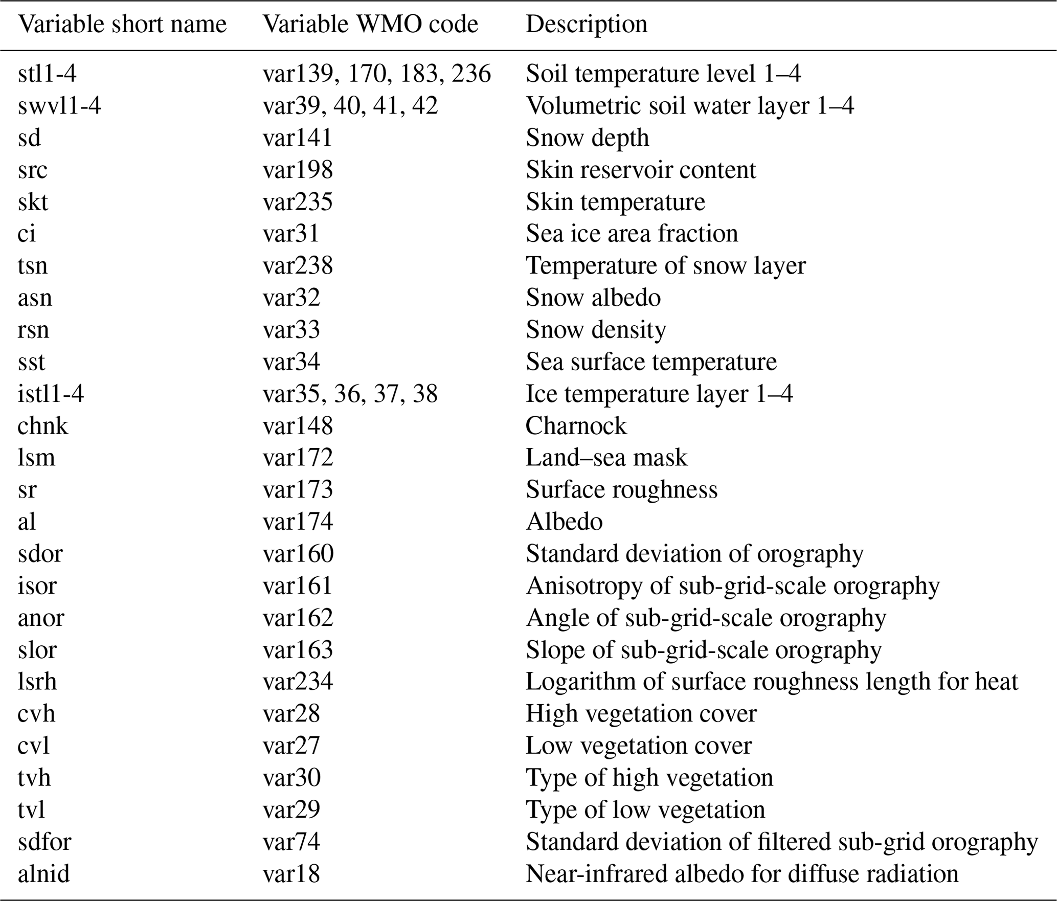
Table A2Model-level variables in spherical harmonics representation in the ICMSHoifsINIT file.

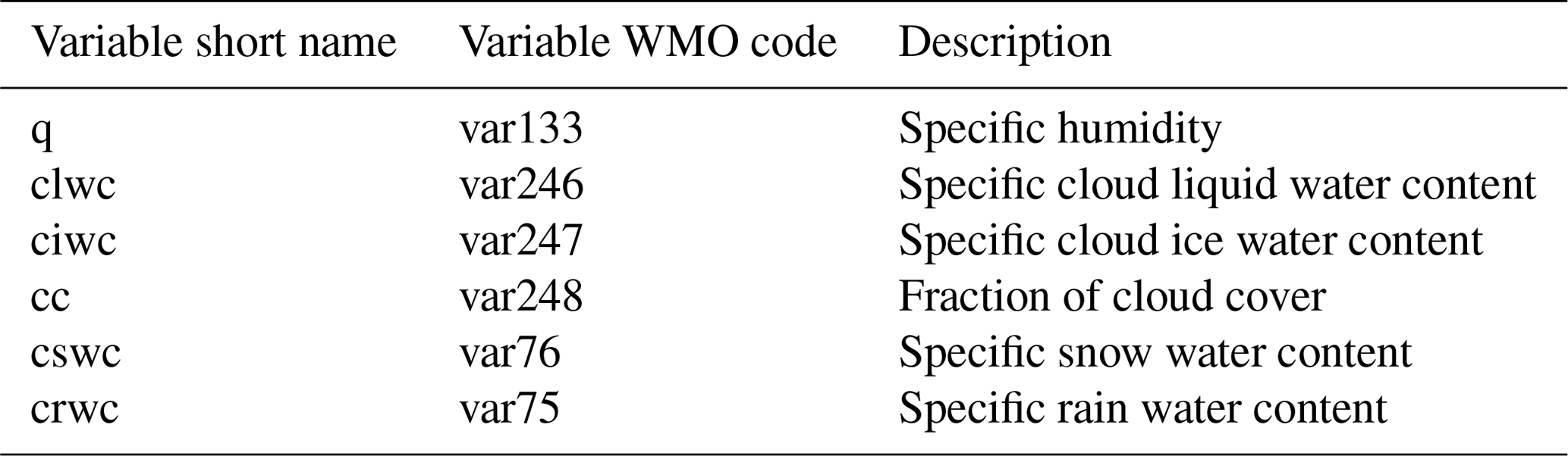
Table A3Model-level variables on a Gaussian reduced grid in the ICMGGoifsINIUA file.
The following gives an example of a workflow in Bash shell with Climate Data Operators (CDO; Schulzweida, 2019; available at https://code.mpimet.mpg.de/projects/cdo, last access: 21 April 2021) when constructing EDA-only initial state perturbations to replace ICMSHoifsINIT. Note that the field subtraction can be done in spherical harmonics representation as well as in grid point space.
-
Convert to grid point representation (cdo -sp2gpl <input file> <output file>)
cdo -sp2gpl ICMSHoifsINIT gg_ctrl
cdo -sp2gpl pua_001 gg_eda+sv
cdo -sp2gp pert_001 gg_sv -
Separate the variable fields (multi-field subtraction not supported)(cdo -selvar,<field names> <input file> <output file>)
cdo -selvar,t gg_eda+sv gg_eda+sv_t
cdo -selvar,d gg_eda+sv gg_eda+sv_d
cdo -selvar,vo gg_eda+sv gg_eda+sv_vo
cdo -selvar,lnsp gg_eda+sv gg_eda+sv_lnsp
cdo -selvar,z gg_eda+sv gg_eda+sv_z
cdo -selvar,t gg_sv gg_sv_t
cdo -selvar,d gg_sv gg_sv_d
cdo -selvar,vo gg_sv gg_sv_vo
cdo -selvar,lnsp gg_sv gg_sv_lnsp -
Change resolution of SV perturbations to match the other fields (cdo -genbil,<grid> <input file> <output file> is used to first generate interpolation weights; cdo -remap,<grid>,<weights> <input file> <output file> then does the interpolation applying these weights.)
cdo -genbil,gg_eda+sv_t gg_sv_t grid
cdo -remap,gg_eda+sv_t,grid gg_sv_t gg_sv_t_hr
cdo -remap,gg_eda+sv_t,grid gg_sv_d gg_sv_d_hr
cdo -remap,gg_eda+sv_t,grid gg_sv_vo gg_sv_vo_hr
cdo -remap,gg_eda+sv_t,grid gg_sv_lnsp gg_sv_lnsp_hr -
Remove SVs
cdo -sub gg_eda+sv_t gg_sv_t_hr gg_eda_t
cdo -sub gg_eda+sv_d gg_sv_d_hr gg_eda_d
cdo -sub gg_eda+sv_vo gg_sv_vo_hr gg_eda_vo
cdo -sub gg_eda+sv_lnsp gg_sv_lnsp_hr gg_eda_lnsp -
Merge variables and transform back into spherical harmonics
cdo -merge gg_eda_t gg_eda_vo gg_eda_d gg_eda_lnsp gg_eda_z gg_eda
cdo -add gg_ctrl gg_eda gg_final
cdo -gp2spl gg_final ICMSHoifsINIT

Figure C1Ensemble mean initial state for MSLP (coloured contours) and 200 hPa wind vectors (blue barbs) at a TL639 resolution on 2 November at 12:00 UTC.
A software licencing agreement with ECMWF is required to access the OpenIFS source distribution; despite the name, it is not provided under any form of open-source software licence. Licence agreements are free, limited to non-commercial use, forbid any real-time forecasting, and must be signed by research or educational organizations. Personal licences are not provided. OpenIFS cannot be used to produce nor disseminate real-time forecast products. ECMWF has limited resources to provide support; therefore, it may temporarily cease issuing new licences if it is deemed difficult to provide a satisfactory level of support. Provision of an OpenIFS software licence does not include access to ECMWF computers nor the ECMWF data archive (other than public datasets).
Other ECMWF software required for use with OpenIFS, such as ecCodes, is available as open-source software using the Apache2 licence and can be downloaded from the ECMWF GitHub repository (see https://github.com/ecmwf, last access: 21 April 2021). The OpenIFS common files can be downloaded from ftp://ftp.ecmwf.int/pub/openifs/ifsdata/ (last access: 11 March 2021).
OpenEPS software is freely available under an Apache 2.0 licence. The version used in this paper can be downloaded from https://doi.org/10.5281/zenodo.3759127 (Ollinaho, 2020a). The latest development versions, including (among other improvements) support for ecWAM activation, are available from https://github.com/pirkkao/OpenEPS (last access: 12 March 2021).
Post-processing scripts used for this study can be found at https://doi.org/10.5281/zenodo.4001495 (Ollinaho, 2020b). The scripts for calculating the skill scores and plotting are also available: https://doi.org/10.5281/zenodo.4001516 (Ollinaho, 2020c).
The dataset described here will be available for the foreseeable future through the https server described in this paper. The ECMWF analysis states used to calculate the skill scores are available through the ECMWF MARS archive for registered users; these states can also be made available upon request from the corresponding author.
PO designed the workflow for reproducing the initial states, manages the repository of the initial states, and coded the workflow manager OpenEPS and post-processing scripts used here. STKL was instrumental in helping to design the reproduction of the initial states. GDC provided crucial guidance with respect to using OpenIFS for ensemble prediction purposes and regarding all the wave model initial files. LT and ME helped to design and test the OpenEPS workflow manager. HJ was influential in the creation of OpenEPS. All authors contributed to writing the paper.
The authors declare that they have no conflict of interest.
The authors would like to thank ECMWF for helping with the publication of this dataset. We are very grateful to an anonymous referee and to Hannah Christensen, who provided insightful and valuable comments that helped to improve this paper. We also want to thank Jean Bidlot from ECMWF for sharing his knowledge regarding the ECMWF wave model. Moreover, the authors are grateful to the CSC-IT Center for Science, Finland, for providing computational resources and to Juha Lento at CSC-IT for helping to design the workflow manager.
This research has been supported by the Academy of Finland, Luonnontieteiden ja Tekniikan Tutkimuksen Toimikunta (grant nos. 316939, 333034, and 1333034). In addition, we warmly acknowledge the support provided by the Vilho, Yrjö and Kalle Väisälä Foundation and by the Doctoral Programme in Atmospheric Sciences of the University of Helsinki.
This paper was edited by Simon Unterstrasser and reviewed by Hannah Christensen and one anonymous referee.
Barkmeijer, J., Buizza, R., Palmer, T. N., Puri, K., and Mahfouf, J.-F.: Tropical singular vectors computed with linearized diabatic physics, Q. J. Roy. Meteor. Soc., 127, 685–708, https://doi.org/10.1002/qj.49712757221, 2001. a
Berner, J., Shutts, G. J., Leutbecher, M., and Palmer, T. N.: A Spectral Stochastic Kinetic Energy Backscatter Scheme and Its Impact on Flow-Dependent Predictability in the ECMWF Ensemble Prediction System, J. Atmos. Sci., 66, 603–626, https://doi.org/10.1175/2008JAS2677.1, 2009. a
Buizza, R.: Localization of optimal perturbations using a projection operator, Q. J. Roy. Meteor. Soc., 120, 1647–1681, 1994. a, b
Buizza, R., Leutbecher, M., and Isaksen, L.: Potential use of an ensemble of analyses in the ECMWF Ensemble Prediction System, Q. J. Roy. Meteor. Soc., 134, 2051–2066, https://doi.org/10.1002/qj.346, 2008. a, b, c
ECMWF: Changes in ECMWF model, available at: https://www.ecmwf.int/en/forecasts/documentation-and-support/changes-ecmwf-model (last access: 21 April 2021), 2019a. a, b
ECMWF: IFS documentation, available at: https://www.ecmwf.int/en/publications/ifs-documentation (last access: 21 April 2021), 2019b. a, b, c
ECMWF: PART VII: ECMWF WAVE MODEL, p. 7, IFS Documentation, available at: https://www.ecmwf.int/node/19311 (last access: 21 April 2021), 2019c. a
ECMWF: OpenIFS CY43R3 release notes, available at: https://confluence.ecmwf.int/display/OIFS/Release+notes+for+OpenIFS+43r3v1 (last access: 21 April 2021), 2020a. a
ECMWF: Severe Event Catalogue, available at: https://confluence.ecmwf.int/display/FCST/201711+-+Tropical+Cyclone+-+Damrey (last access: 21 April 2021), 2020b. a
Ehrendorfer, M. and Tribbia, J.: Optimal prediction of forecast error covariance through singular vectors, J. Atmos. Sci., 54, 286–313, 1997. a
Ferro, C. A. T.: Fair scores for ensemble forecasts, Q. J. Roy. Meteor. Soc., 140, 1917–1923, https://doi.org/10.1002/qj.2270, 2014. a
Friederichs, P., Wahl, S., and Buschow, S.: Chapter 5 – Postprocessing for Extreme Events, in: Statistical Postprocessing of Ensemble Forecasts, edited by: Vannitsem, S., Wilks, D. S., and Messner, J. W., 127–154, Elsevier, https://doi.org/10.1016/B978-0-12-812372-0.00005-4, 2018. a
GFDRR: 2017 Vietnam Post-Typhoon Damrey Rapid Damage and Needs Assessment, available at: https://www.gfdrr.org/sites/default/files/publication/vietnam-damrey-rapid-assessment-report-en.pdf (last access: 21 April 2021), 2018. a
Haiden, T., Janousek, M., Bidlot, J.-R., Ferranti, L., Prates, F., Vitart, F., Bauer, P., and Richardson, D.: Evaluation of ECMWF forecasts, including 2016–2017 upgrades, Technical memorandum, 817, https://doi.org/10.21957/x397za5p5, 2017. a
Lang, S., Hólm, E., Bonavita, M., and Tremolet, Y.: A 50-member Ensemble of Data Assimilations, 27–29, https://doi.org/10.21957/nb251xc4sl, 2019. a, b, c
Lang, S. T. K., Leutbecher, M., and Jones, S. C.: Impact of perturbation methods in the ECMWF ensemble prediction system on tropical cyclone forecasts, Q. J. Roy. Meteor. Soc., 138, 2030–2046, https://doi.org/10.1002/qj.1942, 2012. a, b, c
Lang, S. T. K., Bonavita, M., and Leutbecher, M.: On the impact of re-centring initial conditions for ensemble forecasts, Q. J. Roy. Meteor. Soc., 141, 2571–2581, https://doi.org/10.1002/qj.2543, 2015. a
Lang, S. T. K., Lock, S.-J., Leutbecher, M., Bechtold, P., and Forbes, R. M.: Revision of the SPP model uncertainty scheme in the IFS, Q. J. Roy. Meteor. Soc., 147, 1364–1381, https://doi.org/10.1002/qj.3978, 2021. a
Leutbecher, M.: Ensemble size: How suboptimal is less than infinity?, Q. J. Roy. Meteor. Soc., 145, 107–128, https://doi.org/10.1002/qj.3387, 2019. a, b, c
Leutbecher, M. and Lang, S. T. K.: On the reliability of ensemble variance in subspaces defined by singular vectors, Q. J. Roy. Meteor. Soc., 140, 1453–1466, https://doi.org/10.1002/qj.2229, 2014. a, b, c
Leutbecher, M. and Palmer, T. N.: Ensemble Forecasting, J. Comput. Phys., 227, 3515–3539, 2008. a, b, c, d, e, f, g, h
Leutbecher, M., Lock, S.-J., Ollinaho, P., Lang, S. T. K., Balsamo, G., Bechtold, P., Bonavita, M., Christensen, H. M., Diamantakis, M., Dutra, E., English, S., Fisher, M., Forbes, R. M., Goddard, J., Haiden, T., Hogan, R. J., Juricke, S., Lawrence, H., MacLeod, D., Magnusson, L., Malardel, S., Massart, S., Sandu, I., Smolarkiewicz, P. K., Subramanian, A., Vitart, F., Wedi, N., and Weisheimer, A.: Stochastic representations of model uncertainties at ECMWF: state of the art and future vision, Q. J. Roy. Meteor. Soc., 143, 2315–2339, https://doi.org/10.1002/qj.3094, 2017. a, b
Lock, S.-J., Lang, S. T. K., Leutbecher, M., Hogan, R. J., and Vitart, F.: Treatment of model uncertainty from radiation by the Stochastically Perturbed Parametrization Tendencies (SPPT) scheme and associated revisions in the ECMWF ensembles, Q. J. Roy. Meteor. Soc., 145, 75–89, https://doi.org/10.1002/qj.3570, 2019. a, b
Lorenz, E. N.: A study of predictability of a 28-variable atmospheric model, Tellus, 17, 321–333, 1965. a
Malardel, S., Wedi, N., Deconinck, W., Diamantakis, M., Kühnlein, C., Mozdzynski, G., Hamrud, M., and Smolarkiewicz, P.: A new grid for the IFS, ECMWF Newsletter, 146, 23–28, 2016. a
Ollinaho, P.: pirkkao/OpenEPS: Initial release (Version v0.952), Zenodo, https://doi.org/10.5281/zenodo.3759127, 2020a. a
Ollinaho, P.: pirkkao/OpenEPS_PPro: Tag for Zenodo (Version v0.9), Zenodo, https://doi.org/10.5281/zenodo.4001495, 2020b. a
Ollinaho, P.: pirkkao/nc_plot: Tag for Zenodo (Version v0.9), Zenodo, https://doi.org/10.5281/zenodo.4001516, 2020c. a
Ollinaho, P., Bechtold, P., Leutbecher, M., Laine, M., Solonen, A., Haario, H., and Järvinen, H.: Parameter variations in prediction skill optimization at ECMWF, Nonlin. Processes Geophys., 20, 1001–1010, https://doi.org/10.5194/npg-20-1001-2013, 2013. a
Ollinaho, P., Järvinen, H., Bauer, P., Laine, M., Bechtold, P., Susiluoto, J., and Haario, H.: Optimization of NWP model closure parameters using total energy norm of forecast error as a target, Geosci. Model Dev., 7, 1889–1900, https://doi.org/10.5194/gmd-7-1889-2014, 2014. a
Ollinaho, P., Lock, S.-J., Leutbecher, M., Bechtold, P., Beljaars, A., Bozzo, A., Forbes, R. M., Haiden, T., Hogan, R. J., and Sandu, I.: Towards process-level representation of model uncertainties: stochastically perturbed parametrizations in the ECMWF ensemble, Q. J. Roy. Meteor. Soc., 143, 408–422, https://doi.org/10.1002/qj.2931, 2017. a, b
Palmer, T. N., Gelaro, R., Barkmeijer, J., and Buizza, R.: SVs, metrics and adaptive observations, J. Atmos. Sci., 55, 633–653, 1998. a
Puri, K., Barkmeijer, J., and Palmer, T. N.: Ensemble prediction of tropical cyclones using targeted diabatic singular vectors, Q. J. Roy. Meteor. Soc., 127, 709–731, 2001. a
Rasku, T., Miettinen, J., Rinne, E., and Kiviluoma, J.: Impact of 15-day energy forecasts on the hydro-thermal scheduling of a future Nordic power system, Energy, 192, 116668, https://doi.org/10.1016/j.energy.2019.116668, 2020. a
Schulzweida, U.: CDO User Guide, Zenodo, https://doi.org/10.5281/zenodo.3539275, 2019. a, b
Smith, P., Pappenberger, F., Wetterhall, F., del Pozo, J. T., Krzeminski, B., Salamon, P., Muraro, D., Kalas, M., and Baugh, C.: Chapter 11 – On the Operational Implementation of the European Flood Awareness System (EFAS), in: Flood Forecasting, edited by: Adams, T. E. and Pagano, T. C., Academic Press, 313–348, https://doi.org/10.1016/B978-0-12-801884-2.00011-6, 2016. a
Sperati, S., Alessandrini, S., and Monache, L. D.: An application of the ECMWF Ensemble Prediction System for short-term solar power forecasting, Sol. Energy, 133, 437–450, https://doi.org/10.1016/j.solener.2016.04.016, 2016. a
Tuppi, L., Ollinaho, P., Ekblom, M., Shemyakin, V., and Järvinen, H.: Necessary conditions for algorithmic tuning of weather prediction models using OpenIFS as an example, Geosci. Model Dev., 13, 5799–5812, https://doi.org/10.5194/gmd-13-5799-2020, 2020. a
Yamaguchi, M., Lang, S. T. K., Leutbecher, M., Rodwell, M. J., Radnoti, G., and Bormann, N.: Observation-based evaluation of ensemble reliability, Q. J. Roy. Meteor. Soc., 142, 506–514, https://doi.org/10.1002/qj.2675, 2016. a
- Abstract
- Introduction
- ECMWF OpenIFS
- Initial state perturbations in the ECMWF ensemble
- The dataset
- Running ensembles from the dataset
- Ensemble forecast skill evaluation
- Discussion and conclusions
- Appendix A: Variables contained in initial state files
- Appendix B: Example of manipulating files in spherical harmonics with CDO
- Appendix C: Application to case studies: an example from forecasting a tropical cyclone
- Code and data availability
- Author contributions
- Competing interests
- Acknowledgements
- Financial support
- Review statement
- References