HIDRA 1.0: deep-learning-based ensemble sea level forecasting in the northern Adriatic

Interactions between atmospheric forcing, topographic constraints to air and water flow, and resonant character of the basin make sea level modelling in the Adriatic a challenging problem. In this study we present an ensemble deep-neural-network-based sea level forecasting method HIDRA, which outperforms our set-up of the general ocean circulation model ensemble (NEMO v3.6) for all forecast lead times and at a minuscule fraction of the numerical cost (order of $\mathrm{2}\times {\mathrm{10}}^{-\mathrm{6}}$). HIDRA exhibits larger bias but lower RMSE than our set-up of NEMO over most of the residual sea level bins. It introduces a trainable atmospheric spatial encoder and employs fusion of atmospheric and sea level features into a self-contained network which enables discriminative feature learning. HIDRA architecture building blocks are experimentally analysed in detail and compared to alternative approaches. Results show the importance of sea level input for forecast lead times below 24 h and the importance of atmospheric input for longer lead times. The best performance is achieved by considering the input as the total sea level, split into disjoint sets of tidal and residual signals. This enables HIDRA to optimize the prediction fidelity with respect to atmospheric forcing while compensating for the errors in the tidal model. HIDRA is trained and analysed on a 10-year (2006–2016) time series of atmospheric surface fields from a single member of ECMWF atmospheric ensemble. In the testing phase, both HIDRA and NEMO ensemble systems are forced by the ECMWF atmospheric ensemble. Their performance is evaluated on a 1-year (2019) hourly time series from a tide gauge in Koper (Slovenia). Spectral and continuous wavelet analysis of the forecasts at the semi-diurnal frequency (12 h)⁻¹ and at the ground-state basin seiche frequency (21.5 h)⁻¹ is performed. The energy at the basin seiche in the HIDRA forecast is close to that observed, while our set-up of NEMO underestimates it. Analyses of the January 2015 and November 2019 storm surges indicate that HIDRA has learned to mimic the timing and amplitude of basin seiches.

1 Introduction

Climate change is inducing sea level rise and adversely affects coastal ecosystems, economies and civil safety. In the shallow northern Adriatic, low sea levels influence port activities and inhibit marine cargo while high sea levels cause substantial coastal flooding, inundation and erosion (Ferrarin et al., 2020), thus presenting a serious threat to Venice, Chioggia, Piran and other coastal towns and businesses in the region. Low sea levels predominantly occur when periods of high atmospheric pressure coincide with spring tide sea level minimums. High sea levels typically occur as storm surges during passages of atmospheric cyclones which manifest themselves as substantial air pressure lows and related winds over the basin. Reliable and timely sea level forecasting is thus a crucial element of early warning systems for mitigating the flooding consequences.

Adriatic Sea has an elongated basin with northwest–southeast orientation, lies in the Northern Central Mediterranean and connects to the eastern Mediterranean basin through the Otranto strait at its southern end (see Fig. 1). The basin lies embedded between the Alps (to the north), the Apennines (to the west) and Dinaric Alps (to the east), and it spans a 800 km long and 200 km wide area. The ridges significantly influence the basin circulation through topographic control of the air flow, especially during wind events of Bora (northeasterly wind) and Scirocco (southeasterly wind). Scirocco, predominantly directed along the basin long axis, is among the main drivers of the Adriatic storm surges. The northern Adriatic shelf is closed at its northern end and is the shallowest part of the Adriatic basin. Storm surges in this part are consequently most pronounced, causing substantial coastal flooding, inundation and erosion (Ferrarin et al., 2020).

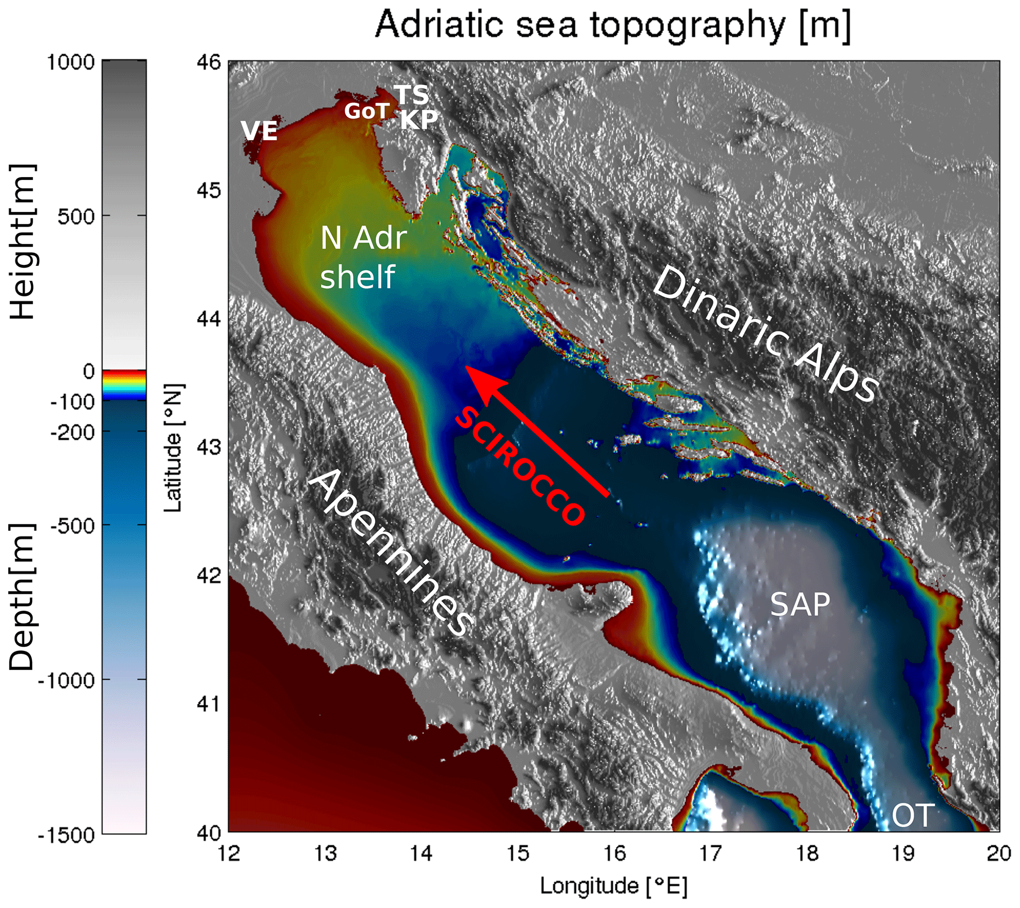
Figure 1 Adriatic orography and bathymetry. The following abbreviations are used: TS – Trieste, KP – Koper, GoT – Gulf of Trieste, VE – Venice, N Adr Shelf – northern Adriatic Shelf, SAP – Southern Adriatic Pit, OT – Otranto Strait. Direction of Scirocco is marked with a red arrow. The image was created by the authors based on EMODnet bathymetry data, available at https://portal.emodnet-bathymetry.eu/ (last access: 27 October 2020), and the Copernicus European Digital Elevation Model, available at https://land.copernicus.eu/imagery-in-situ/eu-dem/eu-dem-v1-0-and-derived-products/eu-dem-v1.0 (last access: 27 October 2020).

The elongated basing results in seiches with a fundamental period of 21.5 h (and first excited mode period of 10.9 h) (Cerovecki et al., 1997; Medvedev et al., 2020). Diurnal and semi-diurnal tides enter the Adriatic through the Otranto Strait and force the basin close to its eigen-periods (Medvedev et al., 2020). Both seiches and tides are resonantly and topographically amplified in the shallow northern Adriatic. In the northern Adriatic, the crest-to-trough range of tidal sea level movement can reach up to 1.5 m (and up to 10 cm s⁻¹ in current speed Cosoli et al., 2013). In the absence of strong winds, this signal dominates the sea level dynamics. During storm surges however, tides are generally too weak to be dominant but remain a crucial part of the total sea level signal. Moreover, since Adriatic seiches decay on scales of several days, seiches and tides may continue to reinforce (or diminish) each other for several days.

The resonant character and high sensitivity to temporal phase lag between tides and seiches make Adriatic sea level prediction a challenge for deterministic numerical ocean models. Even modest modelling errors in the timing, intensity or trajectory of an atmospheric cyclone, often lead to substantial modelling errors in the predicted sea level. The introduction of atmospheric numerical forecast ensembles has thus enabled implementation of operational sea surface height forecast systems that yield probabilistic forecasts along with error variance estimation, which show promise world-wide (see Ferrarin et al., 2020; Bernier and Thompson, 2015; Mel and Lionello, 2014; Bertotti et al., 2011).

These systems, however, often involve a high computational cost, usually requiring running tens of runs of basin-scale numerical ocean models (each forced by a different member of the atmospheric ensemble) each day (or even several times per day). Ensemble numerical modelling is therefore prohibitively demanding for many operational or civil rescue services that lack access to dedicated high-performance computing facilities.

Machine-learning-based ensemble modelling offers a possible solution to the challenges described above. Even though training a machine-learning model may involve a substantial amount of training data and computational resources, the subsequent forecasting – even ensemble forecasting – is numerically cheap enough to be executed in some cases instantaneously on a standard personal computer. Early approaches employ classic machine learning methods (Imani et al., 2018) or shallow fully connected neural networks (Pashova and Popova, 2011; Karimi et al., 2013) for daily or hourly sea level forecasting. The reported results show promise in sea level prediction but fall short with simplistic architectures that ignore the atmospheric forcing. Ishida et al. (2020) attempt to improve the dynamics of hourly-scale sea level forecasts by using a long short-term memory (LSTM) network, which are well established methods for sequence modelling and time-series prediction. The network considers several atmospheric variables (wind speed and direction, sea level pressure, air temperature) as well as relative positions of the Sun and the Moon and annual global air temperatures as the input. Empirically, the short-term sea level prediction of one hour in the future is improved compared to older approaches. While predictions farther into the future could be achieved by iterative auto-regression, the errors would likely exponentially increase. A longer prediction horizon is considered by Braakmann-Folgmann et al. (2017), who apply a combination of recurrent neural networks (LSTMs) and convolutional neural networks to model monthly spatial sea level time series. This is one of the first works that considers both spatial and temporal aspects of the input data; however, predictions are made at a much coarser temporal resolution than that considered in this paper. A higher temporal resolution is considered by Hieronymus et al. (2019), which is the most closely related work to ours. Autoregressive neural networks are used to model the sea level time series with the addition of atmospheric forcing reduced by empirical orthogonal function (EOF) decomposition. For the northern Adriatic, Venice lagoon specifically, artificial neural networks have already been shown to be useful at modelling numerical model errors in sea level prediction (Bajo and Umgiesser, 2010).

In this work we propose HIDRA – a HIgh-performance Deep tidal Residual estimation method using Atmospheric data. HIDRA is a novel deep learning architecture which employs tidal and atmospheric forcing contributions for accurate sea level predictions. The model is trained end-to-end with discriminative feature extraction as part of the learning to maximize the forecast accuracy and to compensate for the inaccuracies of the astronomical tide estimates. HIDRA is benchmarked against the operational set-up of the NEMO v3.6 general circulation model engine (Madec, 2008), which is run daily as part of the National Hydrological Forecasting Service at the Slovenian Environment Agency (ARSO). For brevity, we refer to this particular set-up (see the Code and data availability section for a detailed configuration namelist) as the NEMO model.

The remainder of the paper is structured as follows. The input sea level and atmospheric data and the datasets used in this study are described in Sect. 2. The HIDRA architecture, our NEMO ocean model set-up and the ensemble structure are presented in Sect. 3. Section 4 reports a detailed analysis of the HIDRA architecture and empirical comparison to the NEMO system on a challenging set-up. Conclusions are drawn in Sect. 5.

2 Sea level and atmospheric data

2.1 Sea level data

Sea surface height (SSH) measurements were obtained from the Koper Mareographic Station ($\mathrm{45}{}^{\circ }{\mathrm{33}}^{\prime }$ N, $\mathrm{13}{}^{\circ }{\mathrm{44}}^{\prime }$ E; see Fig. 2 for location), which is operated by the Slovenian Environment Agency (ARSO). The measurements are acquired by a bottom-mounted pressure gauge in 10 min intervals, which are subsequently quality controlled at ARSO. The tidal part of the sea level is independent from atmospheric forcing and can be approximated by tidal models. We analysed the tidal contribution to Koper SSH using the Tidal Analysis Program for Python TAPPY (Cera, 2011). Tidal contribution is estimated from a 20-year hourly time series of Koper SSH for the period between January 1995 and September 2014. Tidal constituents are then used to estimate past and future tidal values. The residual sea level is defined in this paper as the arithmetic difference between the total and the tidal sea level.

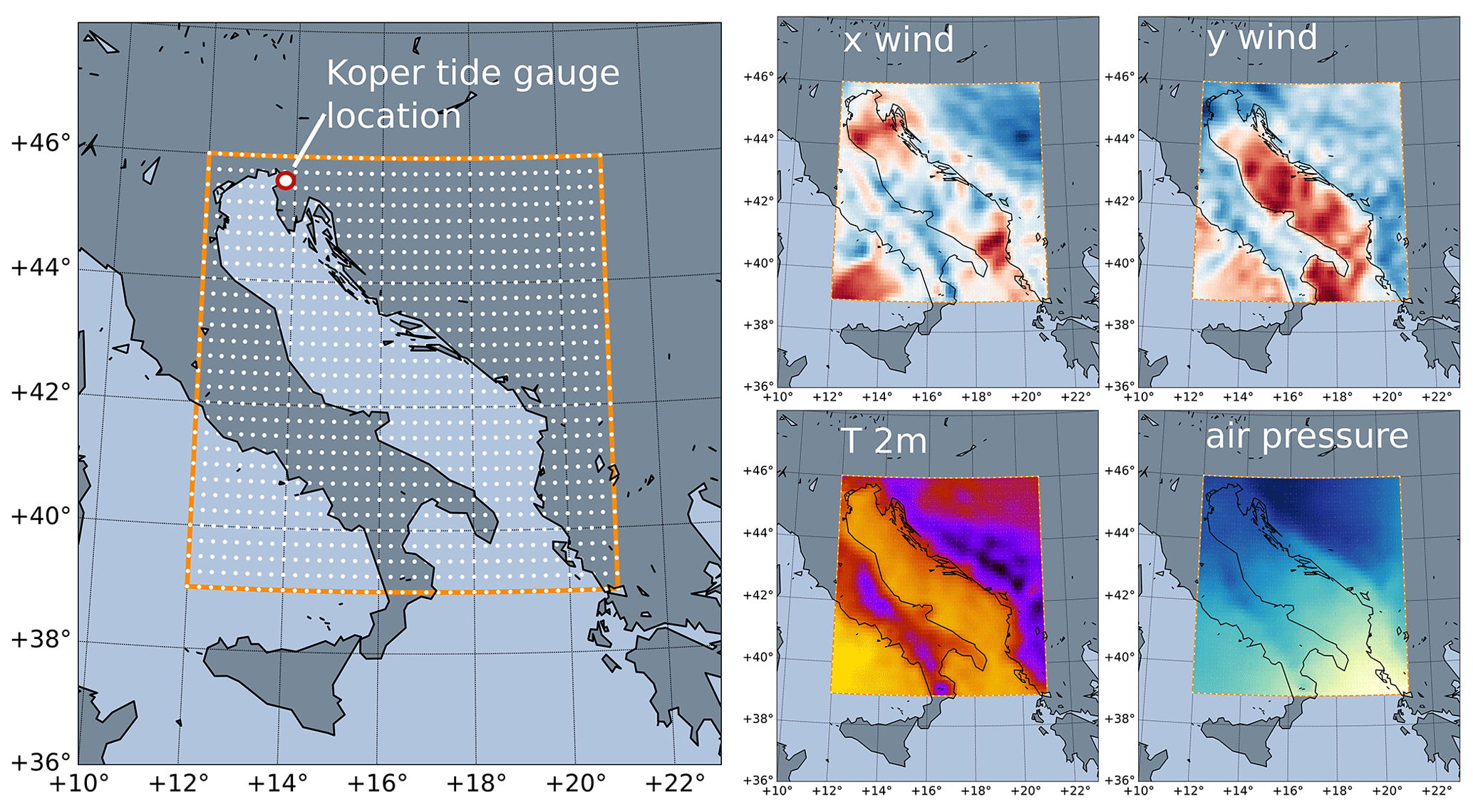
Figure 2 Left: NEMO ocean model domain (orange rectangle) and ECMWF ensemble grid points (white dots). Every second ECMWF grid point is displayed for clarity. Koper tide gauge location is marked with a red–white circle. Right: four ECMWF atmospheric fields are extracted over the region at each time step: zonal (x) and meridional (y) wind, air temperature at 2 m and surface air pressure.

2.2 Atmospheric data

Atmospheric data are obtained from Ensemble Prediction System (EPS) of the European Centre for Medium-Range Weather Forecasts (ECMWF). The data come as an ensemble of 50 integrations of global atmospheric models (Leutbecher and Palmer, 2007). Ensemble forecasts have a 0.125^∘ arc degree spatial (zonal and meridional) resolution and a 3 h temporal resolution. In this study, the following forecast fields were subset to the Adriatic basin, represented by a 73×57 spatial grid (see Fig. 2): (i) 10 m zonal and meridional winds, (ii) mean sea level pressure, and (iii) air temperature at 2 m. The forecasts were linearly interpolated to hourly time steps to match the SSH temporal resolution. Atmospheric fields over land and sea are treated in the same manner; i.e. while HIDRA does receive an explicit spatial encoding of atmospheric fields (Sect. 3.1.1), it does not employ a land–sea mask.

Direct wind influence on the ocean is exerted through vertical momentum transfer or wind stress. Configurations with both raw wind and wind stress were tested to obtain optimal neural network configuration. Whenever wind stress was used, turbulent momentum transfer (wind drag) coefficient was computed using the Large and Pond parametrization (Large and Pond, 1981). Note that the purpose of wind stress parametrization in this study is not to most concisely represent the vertical momentum flux at the ocean surface (which would require more complex schemes), but merely to introduce to the neural network the nonlinear wind stress dependence on the wind to assist its learning process.

2.3 Evaluation datasets

Atmospheric and sea level data described in previous sections were used to create a dataset for the years 2006–2016. The first 80 % of the dataset is used for training (70 %) and validation (10 %), while the last 20 % (September 2014–December 2016) is used for testing. The data are standardized, and global average pooling is used to reduce the dimensionality of the atmospheric data – the spatial dimension of the data in samples is reduced in half, from 73×57 points to 37×29 points, and the temporal dimension of atmospheric data is reduced by a factor of 4. Sea level data retain 1 h resolution. An additional test-only dataset for the year 2019 was constructed in the same manner and was used for comparison of our set-up of NEMO and HIDRA prediction performance.

Oversampling is applied to the training data to improve the prediction accuracy of the rare storm surge events. The training dataset is split into two subsets by thresholding the residuals at 40 cm. Storm surges (residual >40 cm) represent approximately 2 % of the data. During training the samples are randomly sampled from each of the two subsets with equal probability.

3 Numerical models

3.1 HIDRA

HIDRA (a HIgh-performance Deep tidal Residual estimation method using Atmospheric data) is a deep neural network that predicts future surface height residual values (relative to the tidal model) from the sea level and atmospheric forcing input tensors. The atmospheric state at time step t is represented by an atmospheric tensor ${\mathbf{I}}_t\in {\mathcal{R}}^{H\times W\times \mathrm{4}}$, where W=37 and H=29 are the numbers of domain cells in longitudinal and latitudinal directions, respectively. The third dimension of I_t corresponds to the four atmospheric surface input fields: two components of the wind stress, mean sea level pressure and air temperature at 2 m (see Fig. 2).

To account for the causal relation between past atmospheric and tidal forcing in the basin and future sea surface heights, HIDRA considers the forcing data over a range of past and future time steps. In particular, for prediction starting at time t₀, HIDRA takes as the input atmospheric tensors I_t for the interval $t\in [t_{\mathrm{0}}-T_{\text{min}}+\mathrm{1},t_{\mathrm{0}}+T_{\text{max}}]$ and the tidal and the residual values from the interval $t\in [t_{\mathrm{0}}-T_{\text{min}}+\mathrm{1},t_{\mathrm{0}}]$ and predicts residual values for the interval $t\in [t_{\mathrm{0}}+\mathrm{1},t_{\mathrm{0}}+T_{\text{max}}]$. Here, T_min defines the number of past hours considered in sea level prediction and T_max denotes the prediction horizon. In our experiments the predictions are made for 72 h into the future, thus T_max=72 h, and we have determined (see Sect. 4.1.1) that extending the historical horizon beyond 24 h does not affect the prediction accuracy, thus we set T_min=24 h. Note that the atmospheric tensor contains future forecasts as well, while the input sea level vectors contain only tides and residuals observed up to the prediction time t₀.

The HIDRA architecture is summarized in Fig. 3. Atmospheric tensors from all considered time steps are individually encoded by an atmospheric spatial encoder (ASE) module (Sect. 3.1.1) and fused by the temporal encoder block (Sect. 3.1.2) based on the temporal attention mechanism into an atmospheric feature vector. The resulting vector is concatenated with the past tidal and residual measurements. This is followed by a residual regression block (Sect. 3.1.3) to generate the final residual predictions ${\widehat{\mathit{r}}}_t$ along with their uncertainties σ_t.

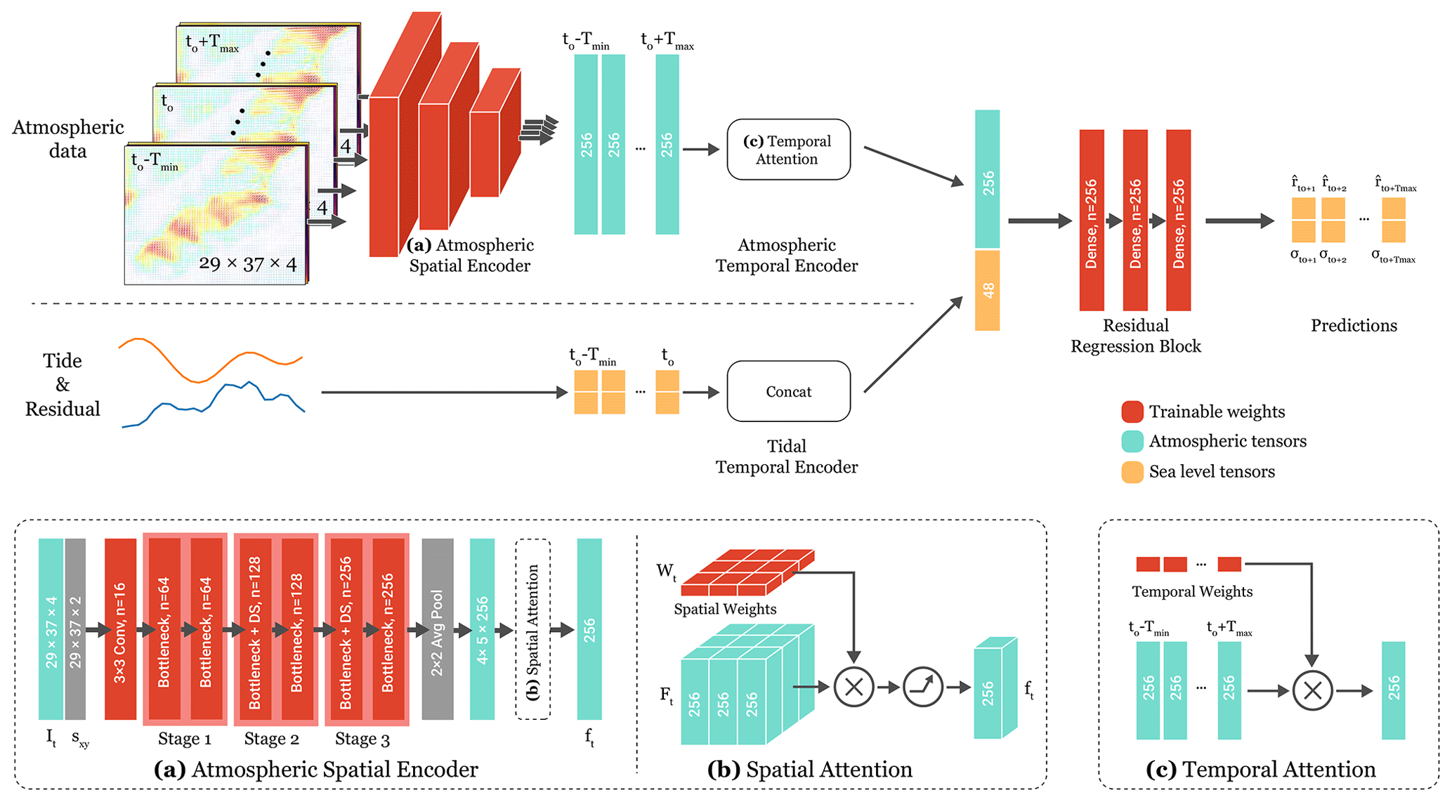
Figure 3 The proposed HIDRA architecture. A convolutional atmospheric spatial encoder (ASE) extracts spatial atmospheric features from each time step. Atmospheric and sea level temporal features are encoded by respective temporal encoder blocks, fused and passed to the fully connected residual regression block to predict the residuals along with their uncertainties. With n we denote the number of filters or units of the block. The trainable blocks are coloured red. The structure of the bottleneck blocks used in the ASE is presented in Fig. 4.

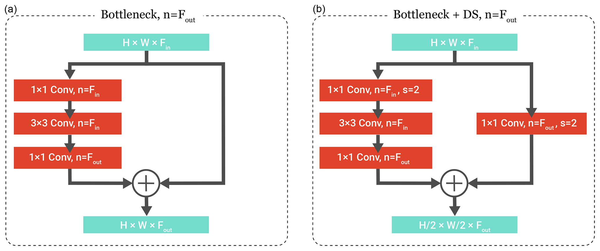
Figure 4 Structure of the bottleneck blocks used in the atmospheric spatial encoder (Fig. 3). The bottleneck block takes a feature map with depth F_in as the input and outputs a feature map with depth F_out. A regular bottleneck block (a) retains the spatial dimensions of the feature maps, while the downsampling (DS) bottleneck block (b) uses strided convolutions to reduce the spatial dimensions in half. We denote the number of convolutional filters by n and the stride parameter by s.

3.1.1 Atmospheric spatial encoder

The atmospheric spatial encoder (ASE) encodes the spatially represented atmospheric data into features, fine-tuned for the task of sea level prediction; i.e. the atmospheric tensor ${\mathbf{I}}_t\in {\mathcal{R}}^{\mathrm{29}\times \mathrm{37}\times \mathrm{4}}$ for time step t is encoded into a feature vector ${\mathit{f}}_t\in {\mathcal{R}}^{\mathrm{256}\times \mathrm{1}}$. The ASE architecture (shown in Fig. 3a) follows design principles of the ResNet20 v2 convolutional neural network (He et al., 2016), which has already demonstrated remarkable performance in image processing tasks. ASE is composed of 22 convolutional layers. Spatial dependence in feature extraction is enforced by concatenating the atmospheric tensor I_t with a spatial encoding tensor $vec{s}_{xy}\in {\mathcal{R}}^{\mathrm{29}\times \mathrm{37}\times \mathrm{2}}$, which contains the x and y coordinates (scaled between 0 and 1) of each pixel in the tensor. The augmented tensor is then processed by a convolutional layer with 16 filters of 3×3 size, followed by three ResNet20 v2 stages, a spatial pooling layer and a time-dependent spatial attention layer (Fig. 3b).

Each ResNet stage consists of two residual (bottleneck) blocks, where each block contains three convolutional layers (i.e. 1×1, 3×3 and 1×1) and a residual connection, which sums the block input with its output. To match the number of output features in the residual connection, the first residual block in each stage uses an additional 1×1 convolutional projection. Spatial feature downsampling (DS) is applied by a stride of length 2 in the first convolutional layer of the second and third stage to increase the effective receptive field of neurons. A ReLU activation layer is appended to each convolutional layer, except for the first one, and prepended by a batch-normalization layer to stabilize the learning.

The output of the last residual block is spatially reduced by half with an average pooling layer, resulting in a feature tensor F_t of size $\mathrm{5}\times \mathrm{4}\times \mathrm{256}$. Finally, a time-dependent spatial attention layer produces the final feature vector ${\mathit{f}}_t\in {\mathcal{R}}^{\mathrm{1}\times \mathrm{256}}$, which is a weighted sum of spatial positions:

$$\begin{array}{}\text{(1)}& {\mathit{f}}_t=\mathrm{ReLU}\left(\sum _{i=\mathrm{1}}^{\mathrm{4}}\sum _{j=\mathrm{1}}^{\mathrm{5}}{\mathbf{F}}_t^{(i,j)}{\mathit{w}}_t^{(i,j)}\right),\end{array}$$

where ${\mathbf{F}}_t^{(i,j)}$ is a slice of the feature tensor at time t at spatial coordinates (i,j), ${\mathit{w}}_t^{(i,j)}$ is the respective spatial weight and ReLU(⋅) is the ReLU activation function. Note that the weight matrices are temporally dependent, which allows them to focus on different parts of the atmospheric feature maps over time. With the exception of the spatial attention layer, all weights of the ASE network are temporally independent and are thus shared between all atmospheric input tensors.

3.1.2 Temporal encoders

The ASE encodes the input sequence of atmospheric tensors into a sequence of atmospheric features. These are stacked into an atmospheric feature matrix $\mathbf{F}\in {\mathcal{R}}^{\mathrm{256}\times T_{\mathrm{\Delta }}}$, where T_Δ is the number of time steps in the atmospheric input tensor I_t, and compressed into a single feature vector $\mathit{f}\in {\mathcal{R}}^{\mathrm{256}\times \mathrm{1}}$ by a weighted summation

$$\begin{array}{}\text{(2)}& \mathit{f}=\mathbf{F}{\mathit{w}}^T,\end{array}$$

where w is a temporal weights vector which serves as a temporal attention mechanism (Fig. 3c) and adjusts the contributions of different past time steps to maximize the prediction performance.

The input tidal and residual sequences, each a T_min×1 vector, are concatenated with the encoded atmospheric feature vector (Eq. 2) into the combined temporally encoded atmospheric and surface height feature vector. This vector is passed to the residual regression block (Sect. 3.1.3) for the final prediction.

3.1.3 Residual regression block

Probabilistic regression is employed to enable the most likely residual values to be predicted along with their uncertainties. For each time step, the mean and variance of a Gaussian probability density function are predicted. The residual regression block output are thus two sequences $\widehat{\mathit{r}}$ and $\widehat{\mathit{\sigma }}$, each a 1×T_max vector, where T_max is the prediction horizon.

The residual regression block (Fig. 3) is composed of three dense fully connected layers, each consisting of 256 units, followed by a fully connected layer that maps into two 1×T_max vectors for the means $\widehat{\mathit{r}}$ and standard deviations $\widehat{\mathit{\sigma }}$. A soft-plus function (Glorot et al., 2011) is applied to the standard deviation vector to ensure positive values.

3.1.4 Network training

A loss function that takes into account the probabilistic outputs is designed for training HIDRA end-to-end. In particular, a log-likelihood of the ground-truth data (i.e. the residuals series ${\mathit{r}}_{t_{\mathrm{0}}}=\mathit{\{}{r}_{t_{\mathrm{0}}+\mathit{\delta }}{\mathit{\}}}_{\mathit{\delta }=\mathrm{0}:T_{\max }}$) is computed under the sequence of predicted Gaussians (Fig. 3, ${\widehat{\mathit{r}}}_{t_{\mathrm{0}}}$ and ${\widehat{\mathit{\sigma }}}_{t_{\mathrm{0}}}$) for all training sequences starting at different times t₀∈𝒯. The loss is thus defined as

$$\begin{array}{}\text{(3)}& \begin{array}{rl}\mathcal{L}(\mathit{r},\widehat{\mathit{r}},\widehat{\mathit{\sigma }})& =-\sum _{t_{\mathrm{0}}\in \mathcal{T}}\sum _{\mathit{\delta }=\mathrm{0}}^{T_{\max }}\log \\ & \left({\displaystyle \frac{\mathrm{1}}{{\widehat{\mathit{\sigma }}}_{t_{\mathrm{0}}+\mathit{\delta }}\sqrt{\mathrm{2}\mathit{\pi }}}}\exp \left({\left(r_{t_{\mathrm{0}}+\mathit{\delta }}-{\widehat{r}}_{t_{\mathrm{0}}+\mathit{\delta }}\right)}^{\mathrm{2}}/{\widehat{\mathit{\sigma }}}_{t_{\mathrm{0}}+\mathit{\delta }}^{\mathrm{2}}\right)\right),\end{array}\end{array}$$

where r are the sets of training samples, while $\widehat{\mathit{r}}$ and $\widehat{\mathit{\sigma }}$ are the corresponding HIDRA predictions and their error estimates, respectively.

The network and experiments are implemented using Google's machine learning library TensorFlow (Abadi et al., 2015). We use the ADAM optimizer with the learning rate of 0.001, β₁=0.9 and β₂=0.999 to train the model. The training batch size is set to 64 data samples. The models are trained for 30 epochs, each epoch consisting of 1000 training steps (batches). A computer with a NVIDIA GeForce GTX 980 graphics card was used for model training and evaluation.

3.2 NEMO ocean model

General circulation model NEMO v3.6 (Madec, 2008) is used as a baseline for comparison with HIDRA. A detailed configuration namelist of our particular set-up described below is available in the supplementary material in the paper.

The Adriatic NEMO model used in this study is set up on a regular longitude–latitude grid (648×504 cells) with a 1${}^{\circ }/\mathrm{72}$ arcdeg horizontal resolution and 31 vertical partial step z^* levels. The model domain spans 12–21^∘ E and 39–46^∘ N (see Fig. 2). In all regions shallower than 2 m, a 2 m depth is enforced. The baroclinic time step was set to 120 s. The barotropic time step is adjusted to meet Courant–Friedrichs–Lewy stability condition. This operational suite runs every day at the Slovenian Environment Agency (ARSO) High Performance Computing Center and is hotstarted from the run of the previous day. Hourly lateral boundary conditions in the Ionian Sea are taken from the hourly Copernicus CMEMS Mediterranean Sea Analysis and Forecast product. Turbulent momentum and heat fluxes across the air–sea interface are parametrized using a CORE bulk flux formulation (Large and Yeager, 2004) and ECMWF ensemble atmospheric fields.

Rivers are modelled as discharge of fresh water at the respective river location as described in Ličer et al. (2016). The Flather boundary condition determines barotropic dynamics at the lateral open boundary, while a flow relaxation scheme (Engedahl, 1995) is applied for baroclinic dynamics and tracers. The lateral momentum boundary condition at the coast is free-slip. The bottom boundary layer is logarithmic with nonlinear bottom friction. Lateral diffusion is governed by Laplacian operators for tracers and dynamics, both operating over geopotential surfaces. A generic length scale k-ϵ scheme is used for vertical diffusion. Surface wave mixing is parametrized using the Craig and Banner formulation (Craig and Banner, 1994). The full NEMO configuration namelist is provided as supplementary material (Žust et al., 2021).

NEMO was run in this study without tidal forcing and predicts the residual sea level for the entire Adriatic basin with the forecast period set to 72 h (as in HIDRA). In the ocean model ensemble simulations, only 8 out of 50 ECMWF ensemble members were used as forcing to our NEMO circulation model due to computational constraints. These eight ensemble members were selected from the full ECMWF ensemble set based on the wind strength from the strongest to the weakest member in steps of 6 (i.e. integer part of $\mathrm{50}/\mathrm{8}$). This generates eight possible forcing scenarios in the Adriatic basin while conserving the wind forecast spread of the reduced ensemble. For the ith ($i=\mathrm{1},\mathrm{\dots },\mathrm{8}$) NEMO ensemble member run, residual sea level forecast for Koper is extracted from the NEMO basin prediction as a single time series. This is then added to the tidal time series, obtained via tidal analysis from observations, to obtain the total modelled sea level, which we denote as y^nemo(i,t).

Each member of the NEMO ensemble sea level forecast for Koper is further corrected for bias. This is necessary to compensate for the fact that NEMO sea level reflects departures from a local geoid and does not represent the absolute local depth of the water, which is also driven by low-frequency processes (like planetary waves in air pressure) which cannot be reflected in the 72 h run in a regional basin. To obtain the absolute sea level needed by port and civil rescue authorities, the NEMO sea level predictions have to be adjusted to the Koper tide gauge observations.

On the nth hour of the forecast day, the model bias with respect to Koper tide gauge observations y^kp(t) is estimated as

$$\begin{array}{}\text{(4)}& {\mathit{ϵ}}_n\left(i\right)=n^{-\mathrm{1}}\sum _{k=\mathrm{1}}^n\left[y^{\mathrm{nemo}}(i,t_k)-y^{\mathrm{kp}}\left(t_k\right)\right].\end{array}$$

The ith ensemble NEMO prediction time series y^nemo(i,t) is then shifted by ϵ_n(i) so that the bias of the first n hours of the $y^{\mathrm{nemo}}(i,\mathrm{1}<t<n)$ with respect to observations is zero. The complete forecast time series y^nemo(i,t) will of course still exhibit a non-zero bias. This procedure is applied every hour as new observations from Koper tide gauge arrive. Note that, unlike the NEMO ensemble, the HIDRA ensemble does not need any such bias correction, because it already contains local tide gauge information through its sea level input in the day prior to the forecast and learns to adjust for the possible bias.

For operational reasons, the first daily NEMO sea level ensemble run usually becomes available between 11:00 and 12:00 UTC at the earliest. This means that the earliest bias correction of each day generally takes into account the first 12 h of tide gauge observations of that day. Raw NEMO time series from the ith ensemble member y^nemo(i,t) therefore gets shifted by ϵ_12h(i) to produce the first bias-corrected forecast of that day, i.e.

$$\begin{array}{}\text{(5)}& y_{\mathrm{bc}\mathrm{12}\mathrm{h}}^{\mathrm{nemo}}(i,t)=y^{\mathrm{nemo}}(i,t)-{\mathit{ϵ}}_{\mathrm{12}\mathrm{h}}\left(i\right),\end{array}$$

with ϵ_12h(i) defined in Eq. (4). The bias-corrected NEMO ensemble mean, ensemble maximum and ensemble minimum time series is then constructed from 12 h bias-corrected ensemble members at each forecast time step in an identical fashion as with HIDRA – see Eqs. (6)–(8). The corresponding time series are denoted as ${\stackrel{\mathrm{‾}}{y}}_{\mathrm{bc}\mathrm{12}\mathrm{h}}\left(t\right)$, $y_{\mathrm{bc}\mathrm{12}\mathrm{h}}^{\max }\left(t\right)$ and $y_{\mathrm{bc}\mathrm{12}\mathrm{h}}^{\min }\left(t\right)$.

3.3 Ensemble statistics

As mentioned in Sect. 2.2, a total of 50 ECMWF atmospheric ensemble members are available daily. This results in an ensemble of n_ens=50 sea level forecasts by HIDRA and an ensemble of n_ens=8 sea level forecasts by NEMO.

The ensemble mean time series is defined as the average overall ensemble members predictions:

$$\begin{array}{}\text{(6)}& \stackrel{\mathrm{‾}}{y}\left(t\right)=n_{\mathrm{ens}}^{-\mathrm{1}}\sum _{i=\mathrm{1}}^{n_{\mathrm{ens}}}y(i,t),\end{array}$$

where y(i,t) is the ith member. Similarly, the ensemble prediction envelope, i.e. the per-time-step minimum and maximum sequence, is defined as

$$\begin{array}{}\text{(7)}& {\displaystyle }{y}^{\max }\left(t\right)=\underset{i}{max}\left[y\right(i,t\left)\right],\text{(8)}& {\displaystyle }{y}^{\min }\left(t\right)=\underset{i}{min}\left[y\right(i,t\left)\right].\end{array}$$

In the interest of clarity, only ensemble means, maximums and minimums, as defined above, are analysed in the following (rather than individual ensemble members).

4 Results and discussion

Predictions from HIDRA and NEMO are discussed in two sections. Section 4.1 analyses the influence of atmospheric and sea level input on HIDRA forecasts and concludes with a brief analysis of HIDRA atmospheric encoder design. Statistical and spectral analyses of HIDRA and NEMO predictions are then presented in Sect. 4.2.

4.1 HIDRA architecture analysis

The HIDRA architecture design choices and their impact on forecast accuracy is analysed in this section. Forecast accuracy is tested (i) with regard to the prediction lead time, i.e. the number of hours in the future we are forecasting, and (ii) with regard to the sea level residual value, i.e. how far away from astronomical tide lies the sea level. All experiments regarding network design are performed on the Koper test sea level dataset, which spans November 2014 to December 2016.

The influence of the historic horizon is examined in Sect. 4.1.1. The contribution of individual data sources (i.e. atmospheric data and sea level history data) is analysed in Sect. 4.1.2. The influence of the residual forecasting approach is evaluated in Sect. 4.1.3. The influence of the proposed atmospheric data encoder in comparison to reconstruction-based empirical orthogonal functions (EOFs) is examined in Sect. 4.1.4, while the influence of the temporal encoder is analysed in Sect. 4.1.5.

4.1.1 Influence of the historic horizon

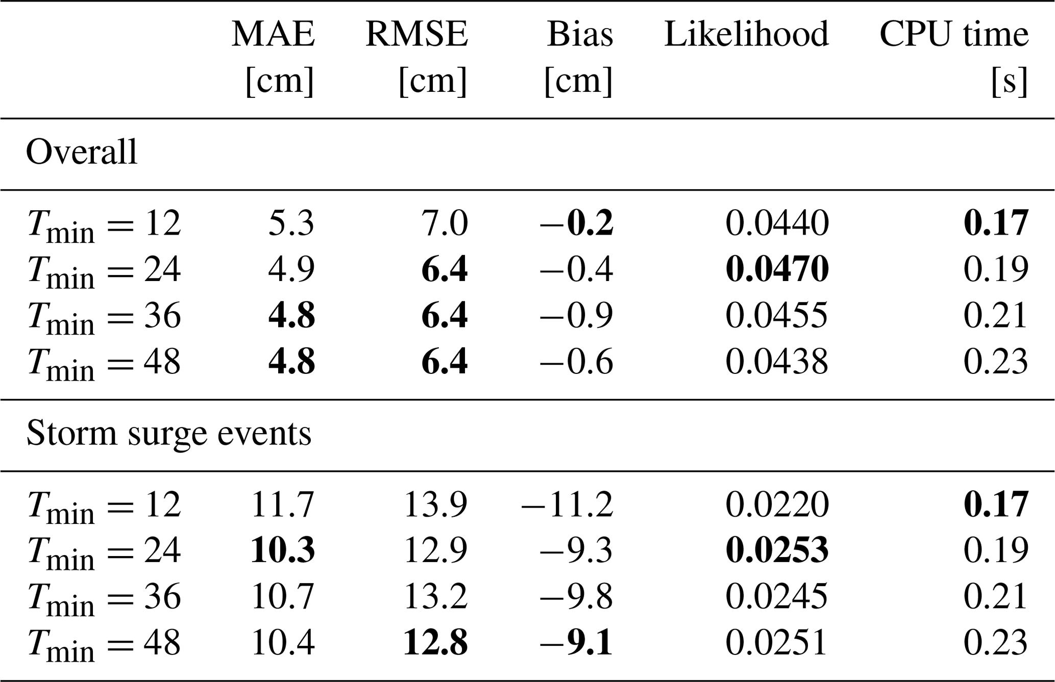
Increasing the length of the historic horizon defined by the parameter T_min (see Sect. 3.1) increases the HIDRA execution time due to a substantially increased number of parameters in the input layer. We therefore analysed the influence of the HIDRA historic horizon length, to find the best trade-off between the model forecast accuracy and the execution time. Table 1 summarizes the performance of HIDRA variants with $T_{\text{min}}\in \mathrm{12},\mathrm{24},\mathrm{36},\mathrm{48}$, which translates to historic horizons of 12, 24, 36 and 48 h prior to the beginning of the forecast. Prediction accuracy substantially increased by increasing the historic horizon from 12 to 24 h (9 % reduction in RMSE) but saturated for larger values. Since we have not observed measurable benefits for horizons beyond 24 h, we have selected T_min=24 as the optimal horizon value. In the remaining analysis, we denote this version as HIDRA₀.

Table 1 HIDRA performance for different historic horizons in terms of mean absolute error (MAE), root mean square error (RMSE), model bias and likelihood shown separately on all data and on storm surge events. CPU execution time (on a single core) per example is also reported. The best result in each category is denoted in bold.

4.1.2 Contribution of atmospheric and sea level inputs

HIDRA uses two input sources: the atmospheric data and the sea level history. In this study we analyse the individual contributions of both input sources. The full HIDRA model (using both atmosphere and sea level data input, denoted as HIDRA₀) is compared with two single-input-source models: (i) HIDRA_Ai, using only atmospheric inputs, and (ii) HIDRA_SLi, using only sea level inputs. In both set-ups, the network branch responsible for processing the ignored input source is removed. Results are presented in Table 2 and Fig. 5.

Table 2 HIDRA performance for individual input data sources in terms of mean absolute error (MAE), root mean square error (RMSE) and model bias. Full HIDRA₀ with both input sources is compared with alternatives that use only atmospheric (HIDRA_Ai) or tidal forcing (HIDRA_SLi) as the input. Performance for the atmospheric tide is provided as reference. Performance is reported on all data as well as on storm surge events only. The best result in each category is denoted in bold.

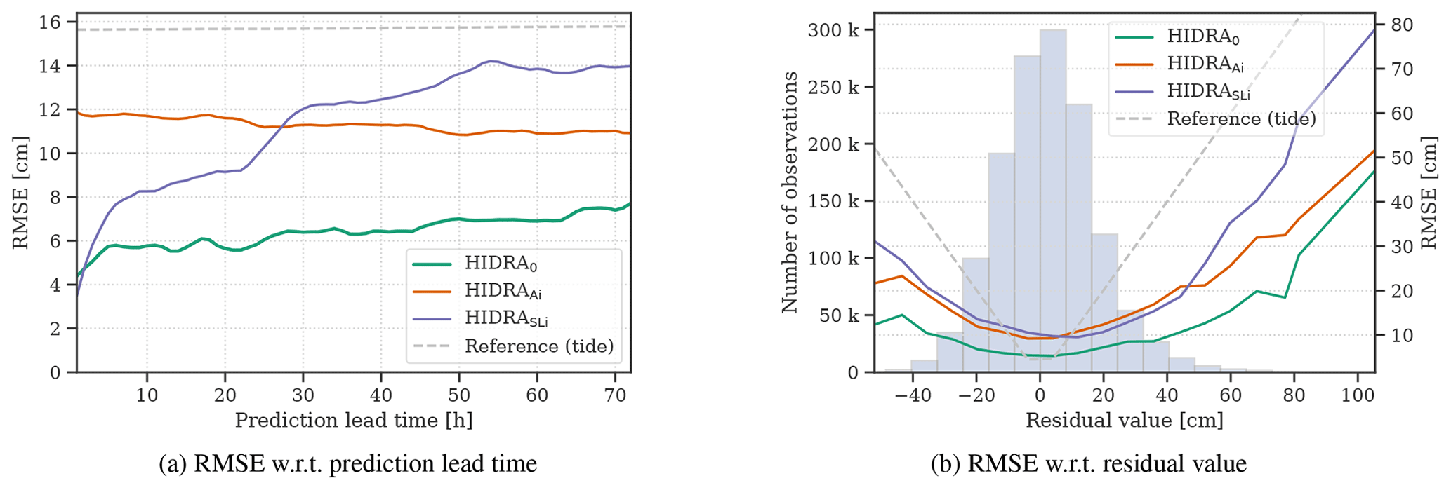
Figure 5 Performance of single-input-source models. Root mean square error (RMSE) with respect to (a) prediction lead time and (b) residual value bins for different input sources is visualized. The full HIDRA model is compared with single-input-source variants – atmospheric data only HIDRA_Ai model and tidal data only HIDRA_SLi model. The RMSE of the astronomic tide is shown for reference.

Table 2 indicates that HIDRA exhibits the best performance when using both atmospheric and sea level input and outperforms both single-source variants by a large margin. This holds overall and also within limited time windows during storm surge events (defined as the timestamps where the residual is larger than 40 cm). Removing each source individually leads to a significant performance drop. The RMSE increases by 77 % when using only the atmospheric input data (HIDRA_Ai), while a 83 % RMSE increase is observed when using only sea level data (HIDRA_SLi). This confirms that both input data sources are essential for accurate prediction. Note also that both input data sources have a similar overall contribution to the prediction accuracy.

Performance analysis over prediction lead time (Fig. 5a) reveals further insights. HIDRA_Ai is very consistent across the entire prediction interval. In fact, the error slightly decreases over time (8 % decrease in RMSE over the interval of 72 h). HIDRA_SLi, on the other hand, is a much better sea level predictor in the short-term, but the error increases rapidly over the prediction interval (by 400 % over the interval of 72 h). Thus, while the sea level data are important for short-term predictions, the atmospheric data are more informative for predictions further into the future.

Grey dashed line in Fig. 5 depicts forecast errors of using the astronomical tide values as the surface height predictor. Since the tidal forecast is done independently of prediction lead time, its RMSE over the prediction time window is simply a root mean square error of the tidal model, plotted as a horizontal line. Bias of the reference tidal model with regard to the specific residual bin is, by definition, the negated value of the residual itself, while its RMSE is, again by definition, simply the absolute value of the residual itself. Whenever HIDRA exhibits lower biases or RMSEs than the tidal reference model, they are essentially predicting more accurately than a tidal model would. Note that this is the case for all prediction lead times and practically all residual values.

On large residual values that correspond to storm surges (Fig. 5b), HIDRA_Ai outperforms HIDRA_SLi, confirming that atmospheric data are essential for accurate storm surge prediction. Both models achieve similar performance on small residual values, and both perform worse than the full model.

4.1.3 Influence of sea level input type

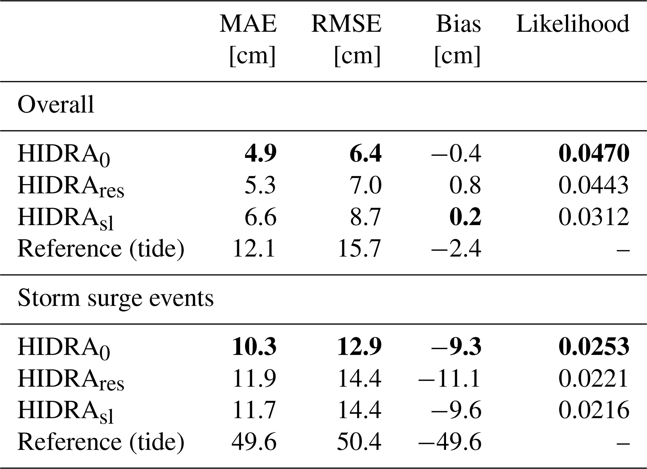
HIDRA considers the total sea level information split into the tide and the residual provided as separate input time series and predicts the residual which is added to the tidal signal to predict the full surface height. To analyse the contribution of different sea level input types, two additional variants were considered: (i) HIDRA_res considered only the residual as the input to predict the future residuals and (ii) HIDRA_sl considered a single total sea level input and predicted the total sea level output.

Results are shown in Table 3. The sea-level-only model (HIDRA_sl) performs significantly worse than the reference HIDRA₀ with a 35 % increase in RMSE, which speaks in favour of residual prediction over the total sea level. The residuals-only model HIDRA_res also performs slightly worse than the full model, causing an 8 % RMSE increase, indicating that tidal information as an additional input provides useful context for improved prediction accuracy.

Table 3 Performance evaluation of different HIDRA sea level input variants. Results are reported for the entire test set (2014–2016) and separately for storm surge events. The best result in each category is denoted in bold.

Performance analysis over different prediction lead times (Fig. 6a) shows that the sea-level-only model HIDRA_sl makes much larger errors (41 % increase compared to HIDRA₀) when predicting far into the future (prediction lead time is high), which suggests that the network has trouble predicting the tidal component that far into the future using only the data from the last 24 h. Comparing predictions over different residual values (Fig. 6b) shows a similar situation. HIDRA_sl performs substantially worse (40 %–50 % larger RMSE than HIDRA₀) for small residual values. This is the range at which the tidal model typically is most accurate and thus provides sufficient information for accurate predictions. Note also that although the sea-level-only model HIDRA_sl does not use tidal information, its prediction errors still follow a similar pattern of increasing with growing residual values. This is an interesting result and shows that the examples belonging to small residual values are inherently easier to predict regardless of whether the tidal estimation is used or not.

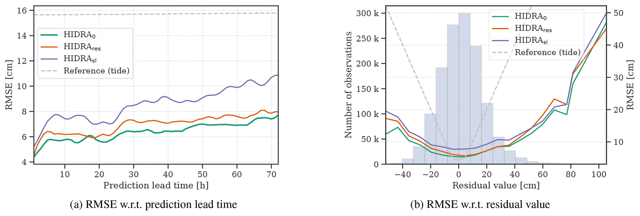
Figure 6 Performance comparison of HIDRA sea level input variants. HIDRA₀ is compared with residuals-only model HIDRA_res, which does not use the estimated tide signal at the input, and the sea-level-only model HIDRA_sl, which does not use separate tidal estimation and predicts the entire sea level signal. The RMSE with respect to (a) prediction lead time and (b) residual value bins is reported. The errors of the astronomic tide are presented for reference.

4.1.4 Influence of the atmospheric encoder

The role of the trainable discriminative atmospheric encoder ASE is analysed by replacing it with a reconstructive embedding proposed in Hieronymus et al. (2019). A principal component analysis is applied to the atmospheric input to compute a low-dimensional subspace (empirical orthogonal functions, EOFs) that maximizes the data reconstruction. Following Hieronymus et al. (2019), the top three EOFs are used in the subspace construction. The input is projected into this subspace producing a low-dimensional signal that is directly used in the HIDRA regression network. The modified HIDRA is denoted by HIDRA_EOF in the following.

Table 4 Comparison of the proposed ASE-based HIDRA₀ and the EOF-based HIDRA_EOF in terms of overall performance and performance on storm surges. The astronomic tide model performance is reported for reference. The best result in each category is denoted in bold.

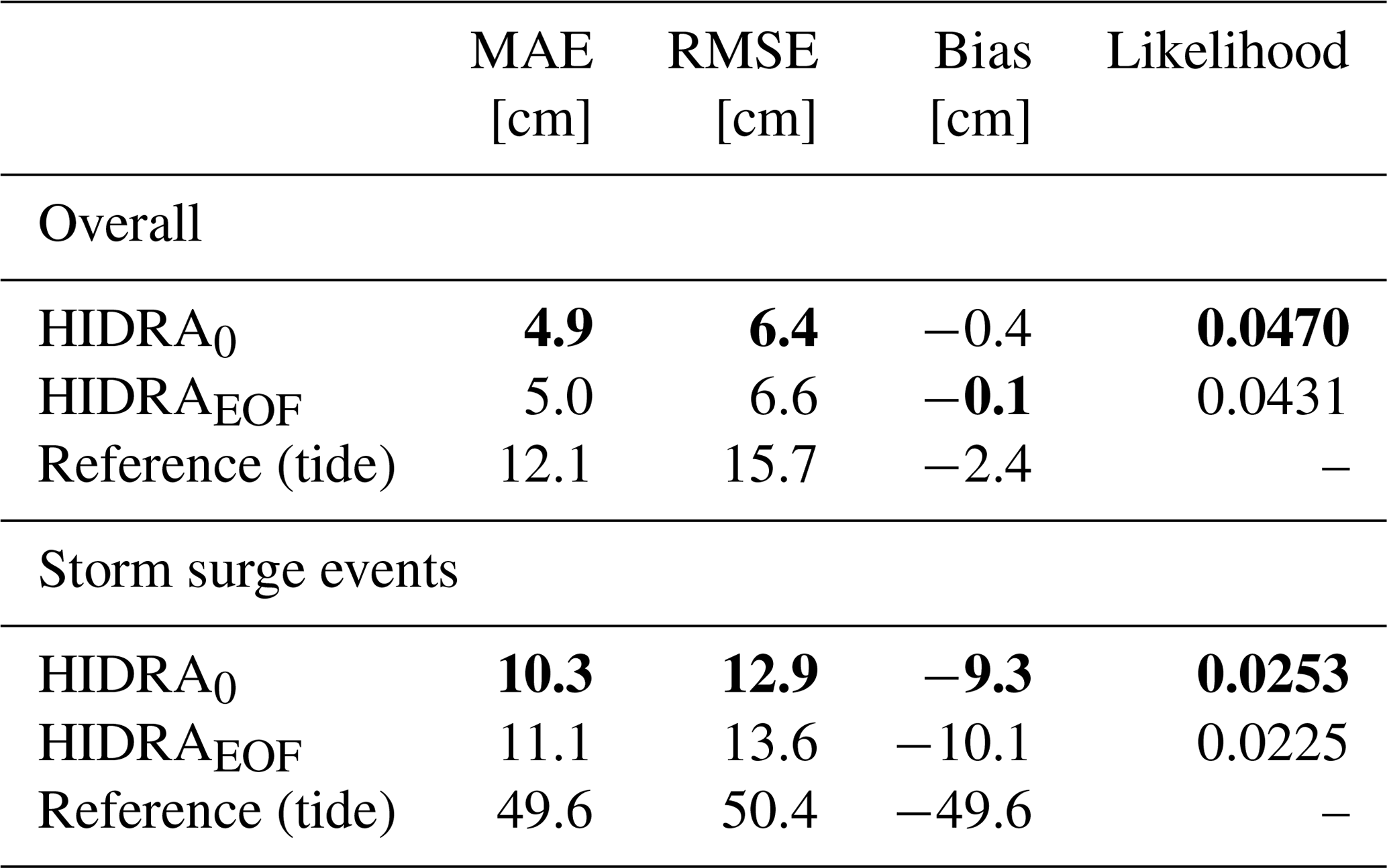
The HIDRA variants with ASE and with EOF are compared in Table 4. In normal conditions, the EOF-based version (HIDRA_EOF) performs on par with HIDRA using the proposed ASE. The HIDRA_EOF RMSE is approximately 3 % larger than that of HIDRA₀. However, the difference increases on the less frequent conditions with high residuals (i.e. surges) in which the EOF-based version results in a 5 % RMSE increase compared to the ASE-based version. This supports the choice of using an end-to-end learned feature encoder as opposed to a hand-crafted one.

4.1.5 Influence of temporal encoders

Temporal encoder with temporal attention weights (Sect. 3.1.2) plays an important part in HIDRA. Two additional variants are created to study alternative choices of feature encoding. The first HIDRA variant (HIDRA_TCN) uses temporal convolutional networks (TCN) (Bai et al., 2018) for encoding the atmospheric and the sea level branch of the network. The atmospheric branch applies three TCN blocks with 128 units, while the sea level branch applies three TCN blocks with 64 units. The second HIDRA variant (HIDRA_LSTM) uses a popular long short-term memory (LSTM) (Hochreiter and Schmidhuber, 1997) networks for temporal encoding. Three LSTM layers are used in both the atmospheric and the sea level branch of the model. Each layer contains 128 units in the atmospheric and 64 in the sea level branch.

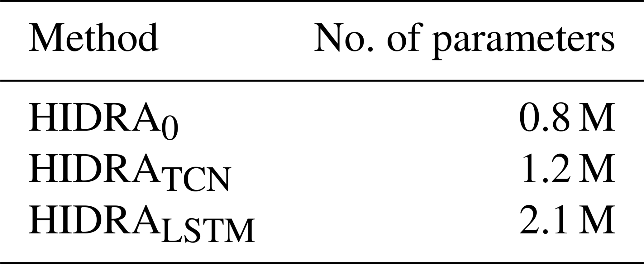
Results are reported in Table 5 and Fig. 7. Overall, HIDRA₀ performs on par with the more complex TCN-based HIDRA_TCN (RMSE of HIDRA_TCN is 3 % larger), while LSTM-based HIDRA_LSTM performs worse (RMSE is 14 % larger than HIDRA₀). HIDRA₀ outperforms both TCN and LSTM-based versions by a solid margin on the storm surge events (31 % and 32 % RMSE increase, respectively). Furthermore, temporal weights of HIDRA₀ use very few parameters compared with the other variants (see Table 6) – TCN and LSTM-based variations increase the total model size (including other network layers) by 50 % and 150 % respectively.

Figure 7 Comparison of different temporal encoder variants. HIDRA₀ is compared with more complex variants using different temporal encoders: LSTMs (HIDRA_LSTM) and TCNs (HIDRA_TCN). The RMSE with respect to (a) prediction lead time and (b) residual values is shown. The prediction errors using the astronomic tide are presented for reference.

Table 5 Performance of HIDRA model variants using different temporal encoders. HIDRA₀ model uses fixed temporal attention for the atmospheric data. HIDRA_TCN uses TCNs and HIDRA_LSTM uses LSTMs to encode temporal features of atmospheric and sea level data. Performance of the astronomic tide is provided for reference. The best result in each category is denoted in bold.

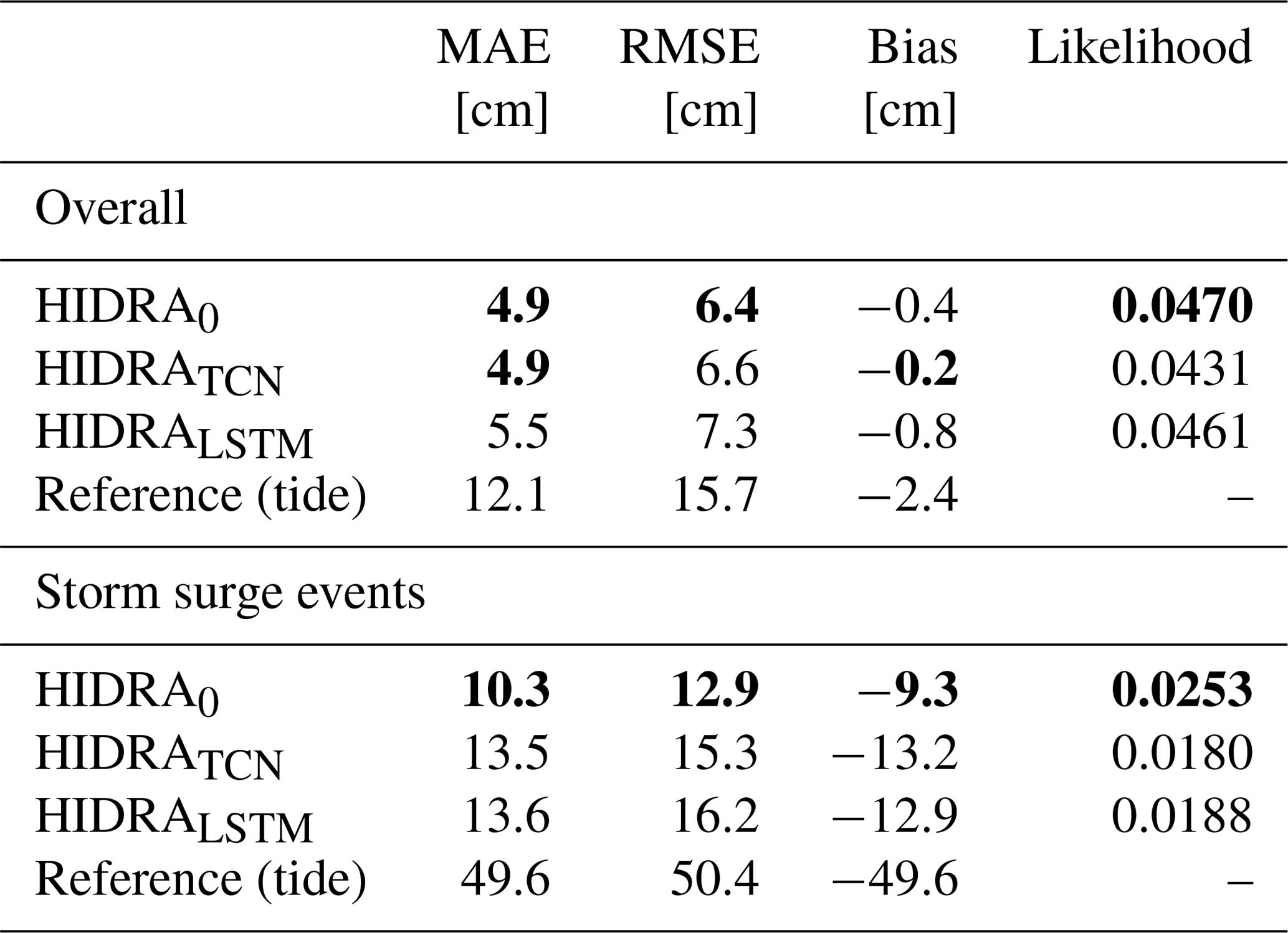
Table 6 Total number (in millions) of trainable parameters of HIDRA variants with different temporal encoders.

4.1.6 Influence of the wind input type and wind-pressure redundancy

Bora and Scirocco characteristics in the Adriatic basin are often determined through an interplay of geostrophic, orographic and other influences (Pasarić et al., 2007; Grisogono and Belušić, 2009). At other times, however, non-geostrophic effects may play a lesser role, and the wind field is largely determined by the pressure field. To investigate potential information redundancy between the wind and pressure inputs, two HIDRA variants were trained: one which did not use the wind input and another which used the wind, but not the pressure. Results in Table 7 show that removing either wind or air pressure input leads to an approximately 9 % increase in RMSE. HIDRA seems to compensate for potential redundancy in the inputs and capitalizes on the fact that wind in the basin is, in the last instance, not entirely pressure driven. In any case using both inputs is preferred.

We proceed to inspect the impact of the Large and Pond parametrization (Large and Pond, 1981) which might oversimplify the wind stress dependence on the wind. To this end we consider another variant of HIDRA, which uses raw wind instead of wind stress. Results in Table 7 show that, overall, the performance between the two wind-input variants is indistinguishable. However, for storm surges, using raw wind reduces the RMSE by approximately 1 cm when compared to the set-up which uses wind stress. It appears that HIDRA is also capable of extracting the information important for sea level prediction during storm surges directly from the raw wind.

Table 7 Performance of HIDRA variants with different wind and pressure input configurations. HIDRA₀ uses the wind stress, HIDRA_wnd uses the raw wind, HIDRA_{no_wnd} does not use wind inputs and HIDRA_{no_prs} uses the wind stress but not the air pressure. Performance of the astronomic tide is provided for reference. The best result in each category is denoted in bold.

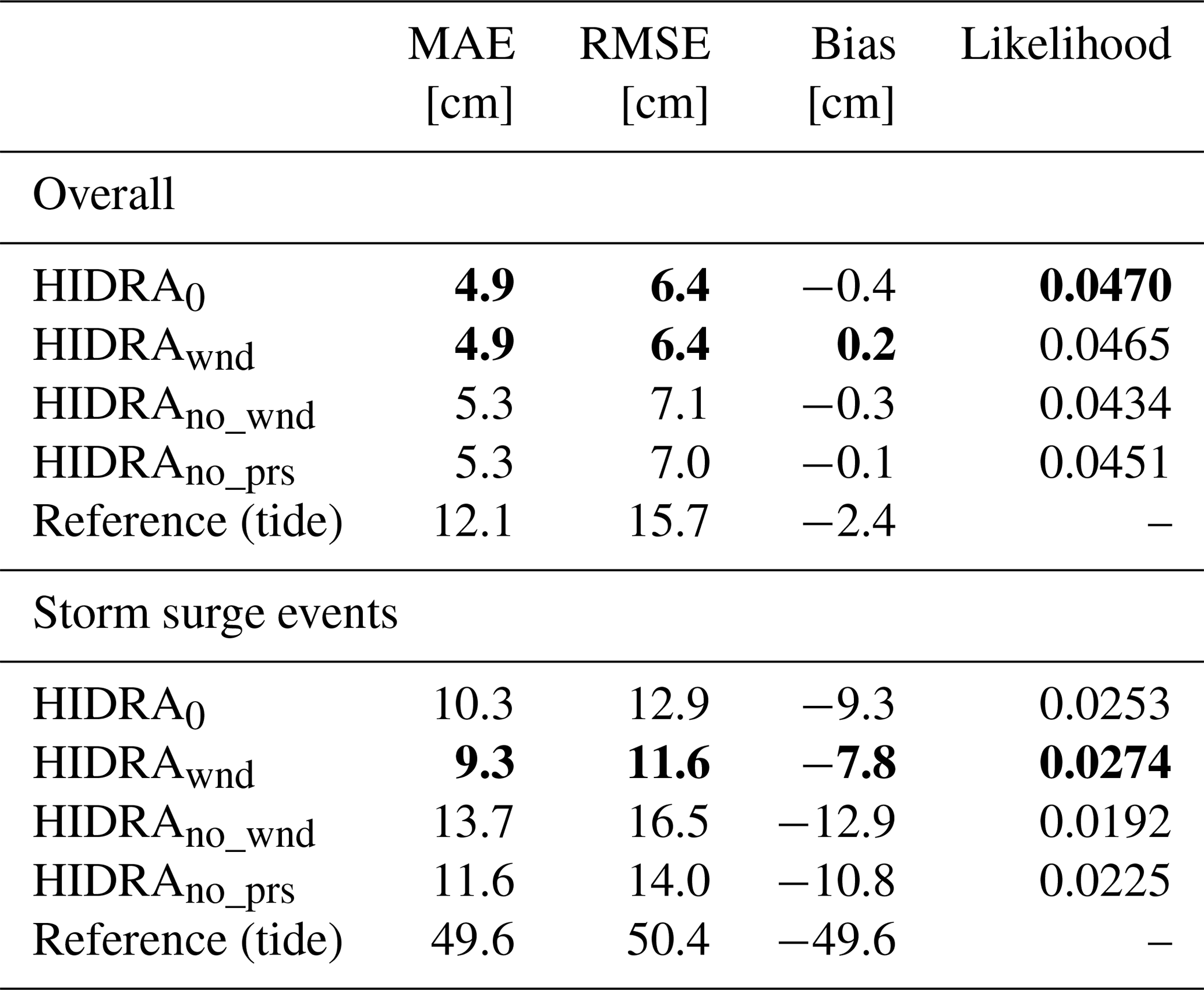
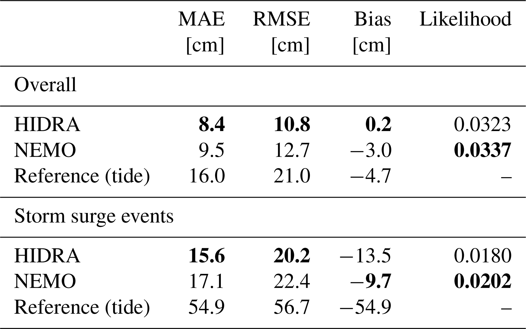
Table 8 Comparison of HIDRA and NEMO on the Koper 2019 test dataset. Overall performance is shown separately from performance during storm surge events. Performance of the astronomic tide is provided for reference. The best result in each category is denoted in bold.

4.2 Comparisons between HIDRA and NEMO

In regional ocean modelling set-ups, tides are often implemented as open boundary conditions and are treated as an external part of model's sea level response. In HIDRA on the other hand, tides enter the model as information that gets inextricably linked into its residual (i.e. non-tidal part of) prediction: results of Sect. 4.1.3 show that including tides improves the prediction of the residual itself. Thus in HIDRA, the quantity we refer to as the residual is in fact composed of two entangled parts: the atmospheric part of the residual and the error correction of the tidal model. We nevertheless use the term residual to differentiate it not from the tide, but rather from total sea level. For these reasons we cannot, as is otherwise customary in sea level modelling, focus on the verification of the residual part of the total sea level signal. In this section, we thus compare the best-performing variant of HIDRA from the ablation study (Sect. 4.1.6) and NEMO on the total sea levels, which, in HIDRA and in NEMO, contain both residuals and tides.

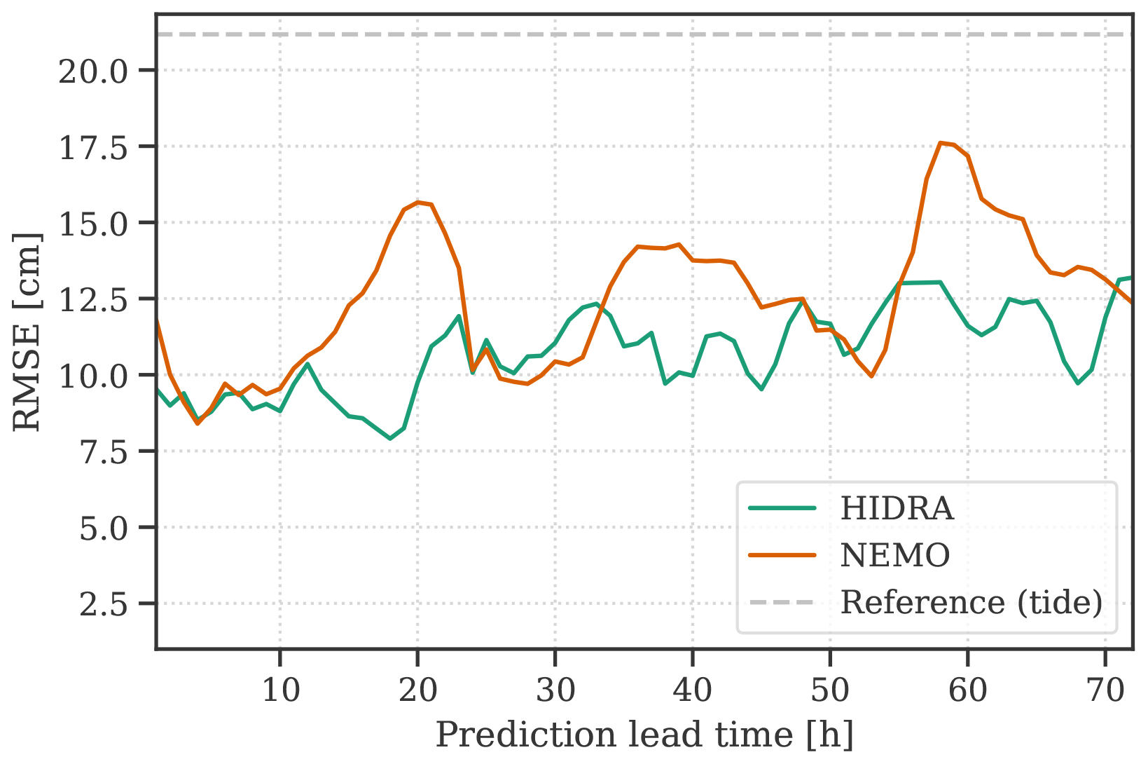
Figure 8 Performance comparison of HIDRA and NEMO with respect to the prediction lead time. Error of the astronomic tide is presented for reference as a grey dashed line.

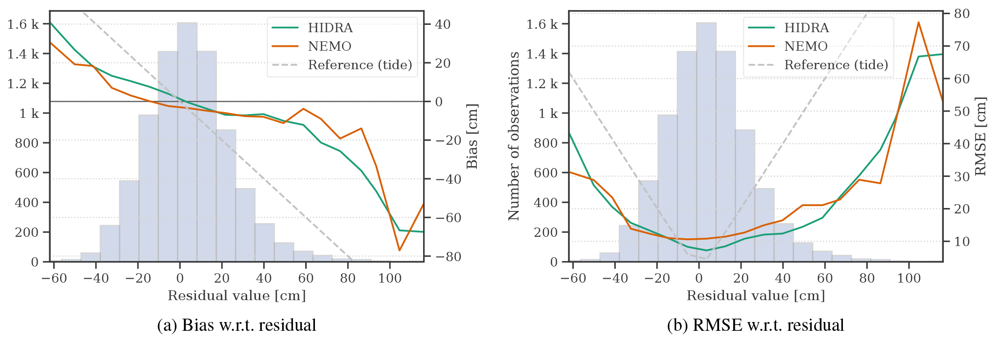
Figure 9 Comparison of HIDRA and NEMO over the sea level distribution. Bias (a) and RMSE (b) with respect to the residual value are shown. Error of the astronomic tide is shown for reference.

4.2.1 Overall performance

HIDRA and NEMO are compared on the 2019 tide-gauge sea level observations in Koper. While HIDRA enables prediction starting at each time step, NEMO does not, since it runs once per day. The models are thus compared only on the prediction windows matching the NEMO runs. The analysis uses the ensemble mean of NEMO members with a 12 h bias correction, i.e. ${\stackrel{\mathrm{‾}}{y}}_{\mathrm{bc}\mathrm{12}\mathrm{h}}\left(t\right)$ defined in Eq. (5). The corresponding ensemble mean HIDRA time series are denoted as ${\stackrel{\mathrm{‾}}{y}}_H\left(t\right)$ and the Koper tide gauge time series are denoted by y^kp(t).

Results are reported in Table 8. Overall (top panel of Table 8), HIDRA outperforms NEMO, obtaining a lower MAE, RMSE and bias. During storm surges (bottom panel of Table 8) HIDRA also outperforms NEMO but exhibits a larger bias. The results visualized with respect to the residual sea level bin in Fig. 9 confirm this. To track the prediction error growth with the prediction horizon, we show RMSE with respect to the prediction lead time in Fig. 8. Both NEMO and HIDRA exhibit a similar RMSE growth trend of approximately +4 cm per 72 h. But NEMO exhibits a higher mean error and a higher error variance. HIDRA outperforms NEMO over the entire range of prediction lead times with lower and less volatile errors.

To gain further insights, the NEMO, HIDRA and tide gauge 2019 time series power spectra were analysed by computing spectral energy densities of the signals over the frequency domain (2 h)⁻¹–(96 h)⁻¹ (Fig. 10). The power spectra were computed as absolute values of one-dimensional fast Fourier transforms. The tide gauge power spectrum exhibits clear tidal presence and also a clear peak at the fundamental Adriatic seiche period of 21.5 h. Some higher harmonics are also present in the tide gauge spectrum at shorter periods (below 8 h) which are present in NEMO but absent from HIDRA. They are, however, less important as they contain at least an order of magnitude less energy than tides or the ground state seiche, which may be the reason HIDRA learned to partially ignore it. Both NEMO and HIDRA contain adequate amounts of energy at tidal periods. But NEMO significantly underestimates the amount of energy contained in the frequency band around the fundamental Adriatic seiche. HIDRA, on the other hand, contains an adequate, if slightly underestimated, amount of energy in the seiche frequency band. This seems to be a solid argument to claim that the network has learned to mimic the fundamental basin seiche behaviour. However, adequate HIDRA energy content in the (21.5 h)⁻¹ frequency band does not in itself mean that Adriatic seiches are excited at appropriate times during storm surge events. To test whether this is indeed the case, inspection of specific storm surge cases is required.

Figure 10 Power spectrum of NEMO ${\stackrel{\mathrm{‾}}{y}}_{\mathrm{bc}\mathrm{12}\mathrm{h}}\left(t\right)$ ensemble forecast mean time series (blue line), HIDRA ensemble forecast mean time series ${\stackrel{\mathrm{‾}}{y}}_H\left(t\right)$ (orange line) and tide gauge observations time series y^kp(t) (black line) for year 2019. Turquoise symbols denote spectral peaks due to respective tidal constituent. E0 denotes the spectral peak due to fundamental Adriatic seiche with a period of 21.5 h, also marked with the vertical turquoise dotted line.

4.2.2 Specific storm surge events

We now proceed to investigate the total sea level time series predicted by NEMO and HIDRA during specific storm surges by analysing the total sea level ensemble envelopes from a 12 h bias-corrected NEMO ${\stackrel{\mathrm{‾}}{y}}_{\mathrm{bc}\mathrm{12}\mathrm{h}}\left(t\right)$ and HIDRA ${\stackrel{\mathrm{‾}}{y}}_H\left(t\right)$. In addition, continuous wavelet transforms (CWTs; see for example Mallat, 2009) over time windows containing the specific storm surges are computed. This allows comparison of the excitation level of specific harmonic contributions to the total sea level during each particular storm surge event. The analysis is focused on the semi-diurnal tidal signal (with periods around 12 h) and on the fundamental seiche period (with a period of 21.5 h). A Morlet wavelet was used for the CWT convolution computation.

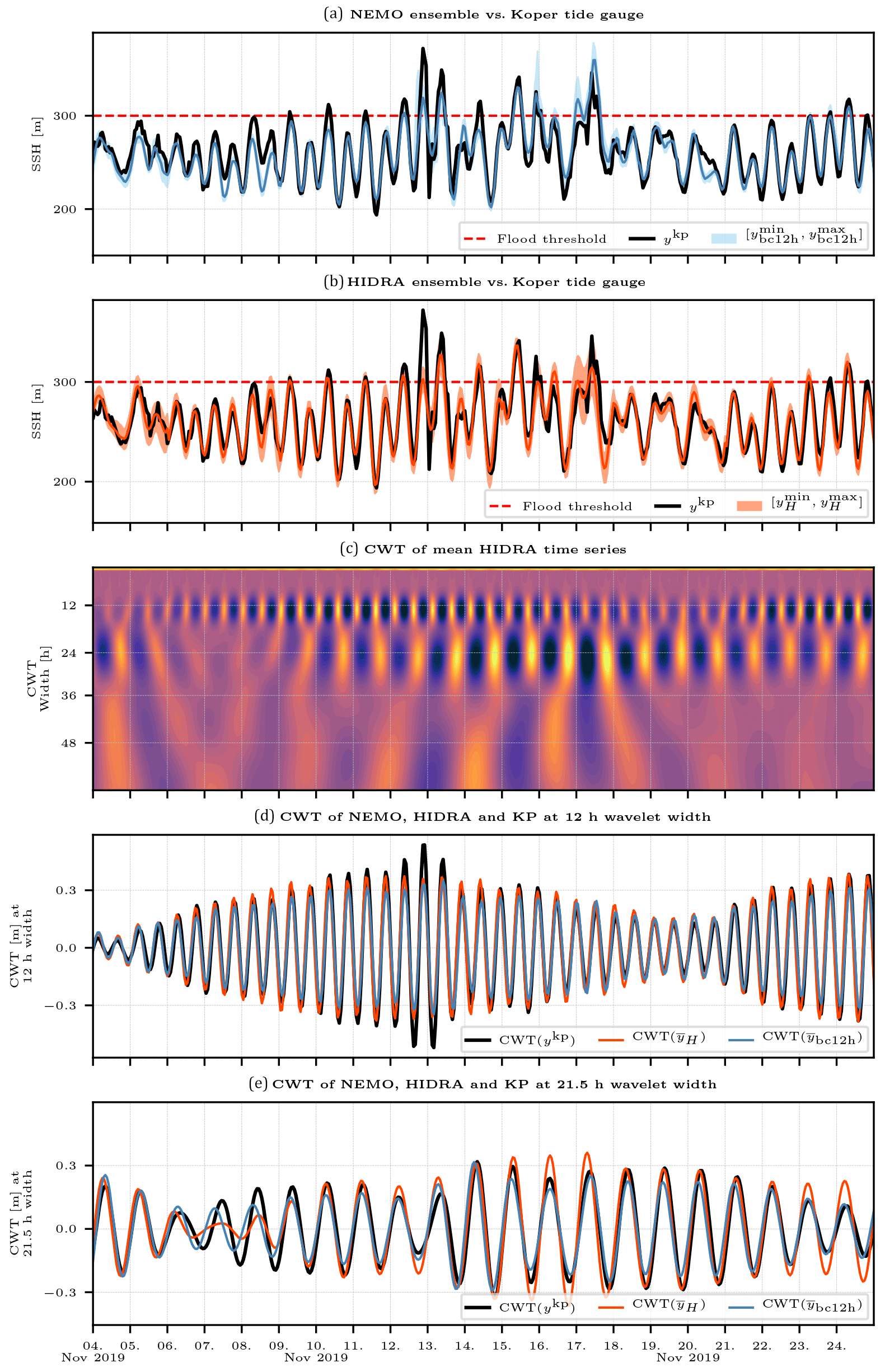
Figure 11 Comparison between NEMO (with a 12 h bias correction) and HIDRA ensembles during a historic surge of November 2019. Panels (a) and (b) depict NEMO and HIDRA ensemble predictions for Koper sea level, together with Koper tide gauge time series. Mean values and minimum–maximum ensemble spans are depicted, as defined in Sect. 3.3. Panel (c) depicts a CWT of ${\stackrel{\mathrm{‾}}{y}}_H\left(t\right)$ HIDRA mean time series. Panels (d) and (e) depict CWTs of Koper tide gauge, HIDRA and NEMO time series at semi-diurnal (12 h) and E0 (21.5 h) wavelet width respectively. The flooding threshold in the historic coastal town of Piran (Slovenia) is marked by a dashed red line in the top two panels.

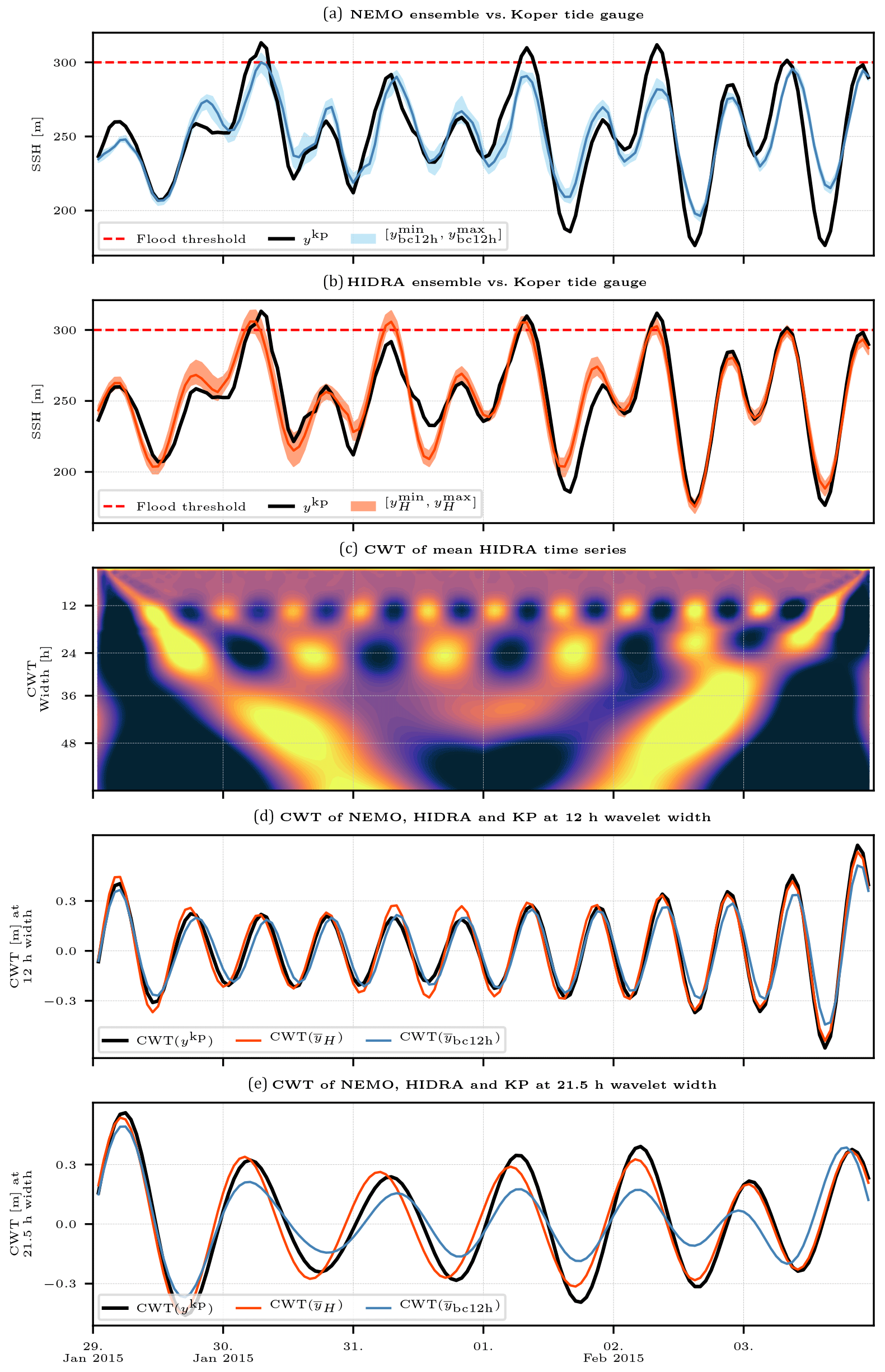
Figure 12 Comparison between NEMO (with a 12 h bias correction) and HIDRA ensembles during a surge of January and February 2015. Panels (a) and (b) depict NEMO and HIDRA ensemble predictions for Koper sea level, together with Koper tide gauge time series. Mean values and minimum–maximum ensemble spans are depicted, as defined in Sect. 3.3. Panel (c) depicts a CWT of ${\stackrel{\mathrm{‾}}{y}}_H\left(t\right)$ HIDRA mean time series. Panels (d) and (e) depict CWTs of Koper tide gauge, HIDRA and NEMO time series at semi-diurnal (12 h) and E0 (21.5 h) wavelet width respectively. Severe flooding threshold in the historic coastal town of Piran (Slovenia) is marked by a dashed red line in the top two panels.

We first discuss the historic storm surge flooding event from mid-November 2019. Atmospheric conditions during November 2019 were not remarkable in themselves. Mean sea level pressures were moving between 990–1000 mbar, while Scirocco speeds in the northern Adriatic were measured to be around 10 ms⁻¹. However, an unfortunate coinciding of a general low pressure, high neap tide and seiche-inducing high-frequency forcing due to a local pressure low caused one of the worst northern Adriatic floods in history (Cavaleri et al., 2020). These multifaceted circumstances made forecasting of these floods, using a lower resolution forcing such as the ECMWF ensemble, challenging (Cavaleri et al., 2020). This problem is at least partly reflected in the November 2019 forecasts, presented in Fig. 11.

Figure 11a depicts NEMO ${\stackrel{\mathrm{‾}}{y}}_{\mathrm{bc}\mathrm{12}\mathrm{h}}\left(t\right)$ mean time series, together with the $y_{\mathrm{bc}\mathrm{12}\mathrm{h}}^{\min }\left(t\right)-y_{\mathrm{bc}\mathrm{12}\mathrm{h}}^{\max }\left(t\right)$ ensemble envelope, while panel (b) depicts HIDRA predictions. Both NEMO and HIDRA mean time series seem to underestimate the storm surge peak values. Both ensembles, however, exhibit high forecast spread, with maximums often adequately representing the observed peaks. The first peak on 12 November 2019 is missed by HIDRA, but the subsequent dynamics is better represented in HIDRA than in NEMO. In particular, HIDRA does not exhibit a substantial false positive on 15 November and also overshoots less during the surge of 17 November 2019. Judging from CWT signals of mean ensembles from both HIDRA and NEMO (in panels d and e), HIDRA missing the first peak can be at least partly attributed to underestimation of semi-diurnal tidal signal in the HIDRA forecast. Semi-diurnal tides are similarly represented in both models and both underestimate the signal in this band. On the other hand the seiche signal seems better represented in HIDRA (panel e) during the storm surge. Note that HIDRA excites the seiche immediately after the sea level peak on 12 November. NEMO, of course, cannot do this since the seiche period is 21.5 h. Figure 11d shows that, like NEMO, HIDRA resolves well the low-frequency tidal variability between spring and neap tides.

We now move to an event from late January and early February 2015, which turned out to be quite problematic for NEMO to forecast, while HIDRA behaved much better. During this period, the Adriatic was impacted by several days of low pressures (990–1000 mbar) and moderate Scirocco (with speeds 8–12 m s⁻¹). These conditions led to a series of moderate storm surges in the northern Adriatic, as shown in Fig. 12.

The NEMO ensemble, depicted in Fig. 12a, performs particularly poorly during this time window. While it did predict the first surge on 30 January, the following peaks were underestimated and the crest-to-trough sea level range of NEMO is overall unsatisfactory throughout the time window. Since the tidal part of the NEMO signal is appropriate (Fig. 12d), the reason for the poor forecast seems to lie in insufficient excitation of the fundamental basin seiche, which is drastically underestimated in our set-up of NEMO (Fig. 12e). HIDRA yields a more accurate overall forecast in this case (Fig. 12b) and does not underestimate the seiche signal at the (21.5 h)⁻¹ frequency as much as NEMO. Semi-diurnal tidal signal is reasonably well represented in both models (Fig. 12d). These performances of NEMO and HIDRA are consistent with the power spectrum in Fig. 10.

5 Conclusions

In this study, we presented HIDRA, a novel deep learning network for sea level modelling in complex environments like the Adriatic. We describe key HIDRA architecture blocks and discuss several aspects of how both HIDRA architecture and its input influence its performance. HIDRA compares favourably to the current operational NEMO set-up of the National Hydrological Forecasting Service at the Slovenian Environment Agency. While further tuning of the operational NEMO set-up at the agency is also under way (with the aim of improving its forecasting skill), results presented in this study nevertheless indicate that HIDRA is an appropriate candidate for the agency's operational pipeline. Preliminary tests (not reported in this study) indicate that HIDRA also generalizes well to other geographical locations.

Last but not least, the numerical cost of both set-ups is vastly different. NEMO ensemble runs require dedicated HPC facilities, while the HIDRA ensemble forecast can be executed on a personal computer (even without a dedicated GPU) and exhibits an extremely low energy footprint. A single HIDRA run for our requirements takes less than half a CPU second per ensemble member, while a full basin NEMO ensemble requires tens of CPU hours per ensemble member – a speedup of the order of 0.5×10⁶ times.

We believe the presented results are a promising first step. In our future work we plan to focus on improving the performance of both HIDRA and NEMO in the tails of the sea level distributions as well as explore other environmental input streams and architectural designs to further reduce the prediction errors with increasing forecast horizon. We hope this study builds a strong case in favour of machine learning capabilities with carefully designed architectures to discern sea level dynamics in regional basins and will inspire other groups to consider similar solutions.