Towards multiscale modeling of ocean surface turbulent mixing using coupled MPAS-Ocean v6.3 and PALM v5.0

A multiscale modeling approach for studying the ocean surface turbulent mixing is explored by coupling an ocean general circulation model (GCM) MPAS-Ocean with the Parallelized Large Eddy Simulation Model (PALM). The coupling approach is similar to the superparameterization approach that has been used to represent the effects of deep convection in atmospheric GCMs. However, the focus of this multiscale modeling approach is on the small-scale turbulent mixing and their interactions with the larger-scale processes in the ocean, so that a more flexible coupling strategy is used. To reduce the computational cost, a customized version of PALM is ported on the general-purpose graphics processing unit (GPU) with OpenACC, achieving 10–16 times overall speedup as compared to running on a single CPU. Even with the GPU-acceleration technique, a superparameterization-like approach to represent the ocean surface turbulent mixing in GCMs using embedded high fidelity and three-dimensional large eddy simulations (LESs) over the global ocean is still computationally intensive and infeasible for long simulations. However, running PALM regionally on selected MPAS-Ocean grid cells is shown to be a promising approach moving forward. The flexible coupling between MPAS-Ocean and PALM allows further exploration of the interactions between the ocean surface turbulent mixing and larger-scale processes, as well as future development and improvement of ocean surface turbulent mixing parameterizations for GCMs.

1 Introduction

Turbulent motions in the ocean surface boundary layer (OSBL) control the exchange of heat, momentum, and trace gases such as CO₂ between the atmosphere and ocean and thereby affect the weather and climate. These turbulent motions are not resolved in regional and global ocean general circulation models (GCMs) due to their small horizontal scales (1–100 m), short temporal scales (10³–10⁵ s), and non-hydrostatic nature. Effects of these subgrid-scale turbulent motions are commonly parameterized in GCMs using simple one-dimensional vertical mixing schemes (e.g., Large et al., 1994; Burchard et al., 2008; Reichl and Hallberg, 2018). However, significant discrepancies are found among many such vertical mixing schemes, highlighting the uncertainties in our understanding of turbulent mixing in the OSBL (Li et al., 2019).

Improvements in OSBL vertical mixing parameterizations will require better constraints under different realistic conditions from either observations or high-fidelity simulations. Due to the scarcity of direct measurements of OSBL turbulence, conventional OSBL parameterization schemes are commonly derived from scaling analysis constrained by high-resolution and non-hydrostatic large eddy simulations (LESs), in which the turbulent motions are resolved, with various initial states and forcing conditions to cover a somewhat realistic parameter space (e.g., Li and Fox-Kemper, 2017; Reichl and Hallberg, 2018; Reichl and Li, 2019). As shown by Li et al. (2019), many OSBL vertical mixing schemes excel at situations in which the scheme was originally derived, but less so in other situations. The problem is that when developing a parameterization for some particular process, we often need to control other factors in order to isolate the effect of that particular process. Essentially, a separation of scales is often assumed and the exploration of the parameter space is often restricted to a certain regime. In reality, processes at different scales interact with each other and the parameter space is vast.

Li et al. (2019) demonstrate a way to consistently evaluate different OSBL vertical mixing schemes over a variety of realistic surface forcing and background stratification conditions. It can also be used to guide a systematic exploration of the parameter space using LES. However, such an approach ignores the interactions between the OSBL turbulence and larger-scale processes, such as submesoscale fronts and eddies, which have been shown to be important (e.g., Hamlington et al., 2014; Bachman and Taylor, 2016; Fan et al., 2018; Verma et al., 2019; Sullivan and McWilliams, 2019).

To study the interactions between the OSBL turbulence and larger-scale processes, simulations that resolve all the important processes across multiple scales are necessary. But they can be extremely computationally expensive. For example, LES that simultaneously resolves the OSBL turbulence and permits some submesoscale features requires a grid size of O(1 m) and a domain size of O(10 km) in the horizontal (e.g., Hamlington et al., 2014; Verma et al., 2019; Sullivan and McWilliams, 2019). Alternatively, the impact of large-scale processes on the small-scale OSBL turbulence can be studied by applying an externally determined large-scale lateral buoyancy gradient in a much smaller LES domain (e.g., Bachman and Taylor, 2016; Fan et al., 2018), though at the expense of missing the feedback to the large scales.

In this work we are building towards a multiscale modeling framework for studying the OSBL turbulent mixing by coupling an ocean GCM, the Model for Prediction Across Scales – Ocean (MPAS-Ocean; Ringler et al., 2013; Petersen et al., 2018), with an LES, the Parallelized Large Eddy Simulation Model (PALM; Raasch and Schröter, 2001; Maronga et al., 2015), effectively running PALM inside the grid cells of MPAS-Ocean. To some extent, this is similar to the superparameterization approach (Randall et al., 2003, 2016), which has long been used in the atmosphere modeling community to represent the effects of cloud by embedding a simplified cloud-resolving model in each grid cell of an atmospheric GCM (Grabowski and Smolarkiewicz, 1999; Khairoutdinov and Randall, 2001; Grabowski, 2004; Randall, 2013) and succeeded in simulating many phenomena that are challenging for conventional cloud parameterizations, such as the diurnal cycle of precipitation and the Madden–Julian oscillation (e.g., Khairoutdinov et al., 2005; Benedict and Randall, 2009). A superparameterization approach in ocean modeling was also explored by Campin et al. (2011) to represent the open-ocean deep convection in a coarse-resolution ocean GCM. However, the primary goal here is not to replace the conventional OSBL vertical mixing parameterizations by an embedded LES, as in a superparameterization-like approach. Instead, we seek to use the coupled MPAS-Ocean and PALM with flexible coupling strategies to systematically study the behavior of OSBL turbulence under different forcing by the larger-scale processes that are resolved in the GCMs, as well as their potential interactions.

Since the small-scale turbulence is a crucial component of the multiscale modeling framework in this study, a high-fidelity three-dimensional LES is required to capture the rich and anisotropic turbulent structures in the OSBL (e.g., McWilliams et al., 1997; Li and Fox-Kemper, 2020). This is different from the traditional superparameterization approach, in which simplified two-dimensional cloud-resolving models (e.g., Grabowski and Smolarkiewicz, 1999; Khairoutdinov and Randall, 2001; Grabowski, 2004) or stochastic reduced models (Grooms and Majda, 2013) are commonly used to represent the bulk effects of the small-scale processes, with some variants, e.g., using two perpendicular sets of narrow channels to partially overcome the two-dimensionality (Jung and Arakawa, 2010). In addition, here we are allowing the embedded LES to run on only selected GCM grid cells, with a loose but flexible coupling with the large-scale GCM fields. Without the computational burden to run LES on every GCM grid cell, we have the flexibility to choose the LES domain and resolution to meet different needs. We note that a similar regional superparameterization approach using LES has recently been explored for the cloud problem (Jansson et al., 2019). Aside from the focus on OSBL turbulence, our approach also differs from theirs by the coupling strategy and the graphics processing unit (GPU) acceleration of the embedded LES (see Sect. 2 for more details).

Simulating processes across scales is a major goal of MPAS-Ocean with its ability to regionally refine the resolution using an unstructured horizontal grid. This allows seamless regionally focused high-resolution simulations, e.g., in the coastal regions, in a large background environment without being nested inside a coarse-resolution simulation. Yet the smallest scale that MPAS-Ocean permits is essentially limited by the hydrostatic assumption. Therefore, coupling with PALM is a natural extension for MPAS-Ocean, which allows for extending multiscale simulations to a smaller scale in which non-hydrostatic dynamics becomes important.

As an initial step towards a multiscale modeling framework of the OSBL turbulent mixing, this paper focuses on the implementation of the framework with some idealized test cases. Rather than focusing on some specific scientific problem, these test cases are chosen to validate the implementation, expose potential issues, and guide future development and applications of the flexible coupling strategy as detailed in the next section. A more sophisticated demonstration of the applications of this framework is left for a future study.

The remainder of this paper is organized as follows. Section 2 describes the multiscale modeling framework to couple MPAS-Ocean with PALM and the approach to accelerate PALM using GPU. The coupled MPAS-Ocean and PALM are then tested in two idealized cases, a single-column case and a mixed layer eddy case, in Sect. 3. The advantages and limitations of this approach, as well as some possible applications moving forward, are discussed in Sect. 4. This paper ends with a brief summary and main conclusions in Sect. 5.

2 Methods

2.1 Coupling MPAS-Ocean with PALM

The Model for Prediction Across Scales – Ocean (MPAS-Ocean, Ringler et al., 2013; Petersen et al., 2018) is the ocean component of the US Department of Energy's Earth system model, the Energy Exascale Earth System Model (E3SM, Golaz et al., 2019). It solves the hydrostatic, incompressible, and Boussinesq primitive equations on an unstructured mesh using finite volume discretization. Model domains may be spherical with realistic bottom topography to simulate the Earth's oceans, or Cartesian for idealized experiments. The Parallelized Large eddy simulation Model (PALM, Raasch and Schröter, 2001; Maronga et al., 2015) is a turbulence-resolving LES model to simulate turbulent flows in the atmospheric and oceanic boundary layers. It solves the non-hydrostatic, incompressible and spatially filtered Navier–Stokes equations with the Boussinesq approximation on a Cartesian grid using finite-difference discretization. It has been widely used to simulate a variety of processes in planetary boundary layers (see Maronga et al., 2015, and the references therein). Both MPAS-Ocean and PALM are under extensive development (see the latest versions at https://github.com/MPAS-Dev/MPAS-Model/releases, last access: 8 April 2021, and https://palm.muk.uni-hannover.de/trac, last access: 8 April 2021). The coupled MPAS-Ocean and PALM presented here are based on MPAS-Ocean version 6.3 and PALM version 5.0.

To illustrate the coupling between MPAS-Ocean and PALM, we write the momentum u and tracer θ equations on a large domain with coarse resolution (denoted by the superscript ()^c) and a small domain with fine resolution (denoted by the superscript ()^f), representing the large-scale dynamics in MPAS-Ocean and small-scale dynamics in PALM, respectively. Essentially, the large-scale momentum and tracers are governed by

$$\begin{array}{ll}\text{(1)}& {\displaystyle }{\partial }_t{\mathit{u}}_{\mathrm{h}}^{\mathrm{c}}& {\displaystyle }=-{\mathit{u}}_{\mathrm{h}}^{\mathrm{c}}\cdot {\mathrm{\nabla }}_{\mathrm{h}}^{\mathrm{c}}{\mathit{u}}_{\mathrm{h}}^{\mathrm{c}}-f\widehat{\mathit{z}}\times {\mathit{u}}_{\mathrm{h}}^{\mathrm{c}}{\displaystyle }& {\displaystyle }-{\displaystyle \frac{\mathrm{1}}{{\mathit{\rho }}_{\mathrm{0}}}}{\mathrm{\nabla }}_{\mathrm{h}}^{\mathrm{c}}{p}^{\mathrm{c}}+{\mathit{d}}_{\mathrm{h}}^{\mathrm{c}}+{\mathit{F}}_{\text{SS}}^{{\mathit{u}}_{\mathrm{h}}},\\ \text{(2)}& {\displaystyle }{\partial }_t{\mathit{\theta }}^{\mathrm{c}}& {\displaystyle }=-{\mathit{u}}_{\mathrm{h}}^{\mathrm{c}}\cdot {\mathrm{\nabla }}_{\mathrm{h}}^{\mathrm{c}}{\mathit{\theta }}^{\mathrm{c}}+s^{\mathrm{c}}+F_{\text{SS}}^{\mathit{\theta }},\end{array}$$

where f is the Coriolis parameter, $\widehat{\mathit{z}}$ is the vertical unit vector, ρ₀ is the reference density, p is the pressure, d is the momentum dissipation, and s is the tracer sources and sinks. A subscript ()_h represents the horizontal components of a vector, e.g., $\mathit{u}=[{\mathit{u}}_{\mathrm{h}},w]$ and $\mathrm{\nabla }=[{\mathrm{\nabla }}_{\mathrm{h}},{\partial }_z]$. The hydrostatic balance,

$$\begin{array}{}\text{(3)}& \mathrm{0}=-{\displaystyle \frac{\mathrm{1}}{{\mathit{\rho }}_{\mathrm{0}}}}{\partial }_z{p}^{\mathrm{c}}+b^{\mathrm{c}},\end{array}$$

is assumed in the vertical, where b is the buoyancy determined by the tracers from the equation of state. The superscript ()^c effectively represents the low-pass-filtered fields with a spatial scale greater than the grid scale of MPAS-Ocean. ${\mathit{F}}_{\text{SS}}^{{\mathit{u}}_{\mathrm{h}}}$ and $F_{\text{SS}}^{\mathit{\theta }}$ represent the small-scale (subgrid-scale) forcings that are not resolved in MPAS-Ocean. Note that here scale separation is assumed only in the horizontal directions, though unlike previous studies, we are not assuming a shared vertical coordinate between the large and small scales so that an interpolation in the vertical is necessary (see more discussions later in this section). Similarly, the small-scale momentum and tracers are governed by

$$\begin{array}{}\text{(4)}& {\displaystyle }\begin{array}{rl}{\partial }_t{\mathit{u}}^{\mathrm{f}}=& -{\mathit{u}}^{\mathrm{f}}\cdot {\mathrm{\nabla }}^{\mathrm{f}}{\mathit{u}}^{\mathrm{f}}-f\widehat{\mathit{z}}\times {\mathit{u}}^{\mathrm{f}}\\ & -{\displaystyle \frac{\mathrm{1}}{{\mathit{\rho }}_{\mathrm{0}}}}{\mathrm{\nabla }}^{\mathrm{f}}{p}^{\mathrm{f}}+b^{\mathrm{f}}\widehat{\mathit{z}}+{\mathit{d}}^{\mathrm{f}}+{\mathit{F}}_{\text{LS}}^{\mathit{u}},\end{array}\text{(5)}& {\displaystyle }{\mathrm{\nabla }}^{\mathrm{f}}\cdot {\mathit{u}}^{\mathrm{f}}=\mathrm{0},\text{(6)}& {\displaystyle }{\partial }_t{\mathit{\theta }}^{\mathrm{f}}=-{\mathit{u}}^{\mathrm{f}}\cdot {\mathrm{\nabla }}^{\mathrm{f}}{\mathit{\theta }}^{\mathrm{f}}+s^{\mathrm{f}}+F_{\text{LS}}^{\mathit{\theta }}.\end{array}$$

The superscript ()^f here represents the total fields with fine resolution but in a limited PALM domain. So that the following constraints need to be satisfied at each MPAS-Ocean grid cell to ensure consistency between the large-scale and small-scale fields,

$$\begin{array}{}\text{(7)}& {\displaystyle }\stackrel{\mathrm{‾}}{{\mathit{u}}_{\mathrm{h}}^{\mathrm{f}}}& {\displaystyle }={\mathit{u}}_{\mathrm{h}}^{\mathrm{c}},\text{(8)}& {\displaystyle }\stackrel{\mathrm{‾}}{{\mathit{\theta }}^{\mathrm{f}}}& {\displaystyle }={\mathit{\theta }}^{\mathrm{c}},\end{array}$$

where $\stackrel{\mathrm{‾}}{\left(\right)}$ is the horizontal average over the PALM domain. Here we assume $\stackrel{\mathrm{‾}}{w^{\mathrm{f}}}=\mathrm{0}$. ${\mathit{F}}_{\text{LS}}^{\mathit{u}}$ and $F_{\text{LS}}^{\mathit{\theta }}$ represent the large-scale forcings that come from MPAS-Ocean. Note that we are not explicitly writing out the subgrid-scale fields in PALM, which occur at a much smaller scale, though we account for their contributions in, for example, the turbulent momentum and tracer fluxes.

Different levels of tightness in the coupling are achieved by combinations of different ${\mathit{F}}_{\text{SS}}^{{\mathit{u}}_{\mathrm{h}}}$, $F_{\text{SS}}^{\mathit{\theta }}$, ${\mathit{F}}_{\text{LS}}^{\mathit{u}}$, and $F_{\text{LS}}^{\mathit{\theta }}$. For ${\mathit{F}}_{\text{SS}}^{{\mathit{u}}_{\mathrm{h}}}$ and $F_{\text{SS}}^{\mathit{\theta }}$, the horizontal and vertical components are often parameterized separately in GCMs due to the large aspect ratio of the grid cell (the horizontal extent of a cell over the vertical). They often represent the effects of different processes, such as mesoscale eddies, which contribute mostly to the horizontal fluxes, and submesoscale eddies and boundary layer turbulence, both of which contribute mostly to the vertical fluxes. Thus, scale separation of the dynamics among multiple scales may be necessary. For the purpose here of representing the ocean surface vertical turbulent mixing in GCMs, we only explicitly consider the vertical component of ${\mathit{F}}_{\text{SS}}^{{\mathit{u}}_{\mathrm{h}}}$ and $F_{\text{SS}}^{\mathit{\theta }}$ in Eqs. (1) and (2), while leaving the horizontal component being parameterized by other routines in MPAS-Ocean. The vertical component of ${\mathit{F}}_{\text{SS}}^{{\mathit{u}}_{\mathrm{h}}}$ and $F_{\text{SS}}^{\mathit{\theta }}$ can be estimated from the vertical convergence of momentum and tracer fluxes in PALM by

$$\begin{array}{}\text{(9)}& {\displaystyle }{\mathit{F}}_{\text{VSS}}^{{\mathit{u}}_{\mathrm{h}}}& {\displaystyle }=-{\partial }_z\stackrel{\mathrm{‾}}{w^{f^{\prime }}{\mathit{u}}_{\mathrm{h}}^{f^{\prime }}},\text{(10)}& {\displaystyle }{F}_{\text{VSS}}^{\mathit{\theta }}& {\displaystyle }=-{\partial }_z\stackrel{\mathrm{‾}}{w^{f^{\prime }}{\mathit{\theta }}^{f^{\prime }}},\end{array}$$

where $({)}^{\prime }=()-\stackrel{\mathrm{‾}}{\left(\right)}$ is the fluctuation around the PALM domain average. In our implementation, we also account for the contributions of subgrid-scale fluxes, and these fluxes are also averaged over an MPAS-Ocean time step (the coupling period). Note that Eqs. (9) and (10) are consistent with conventional parameterizations of vertical mixing, such as the K-profile parameterization (KPP; Large et al., 1994; Van Roekel et al., 2018), in which the fluxes are parameterized.

The most straightforward way to enforce Eqs. (7) and (8) is using relaxing terms for ${\mathit{F}}_{\text{LS}}^{\mathit{u}}$ and $F_{\text{LS}}^{\mathit{\theta }}$,

$$\begin{array}{}\text{(11)}& {\displaystyle }{\mathit{F}}_{\text{LS}}^{\mathit{u}}& {\displaystyle }={\displaystyle \frac{{\mathit{u}}_{\mathrm{h}}^{\mathrm{c}}-\stackrel{\mathrm{‾}}{{\mathit{u}}_{\mathrm{h}}^{\mathrm{f}}}}{{\mathit{\tau }}_{\text{LS}}^{\mathit{u}}}},\text{(12)}& {\displaystyle }{F}_{\text{LS}}^{\mathit{\theta }}& {\displaystyle }={\displaystyle \frac{{\mathit{\theta }}^{\mathrm{c}}-\stackrel{\mathrm{‾}}{{\mathit{\theta }}^{\mathrm{f}}}}{{\mathit{\tau }}_{\text{LS}}^{\mathit{\theta }}}},\end{array}$$

where ${\mathit{\tau }}_{\text{LS}}^{\mathit{u}}$ and ${\mathit{\tau }}_{\text{LS}}^{\mathit{\theta }}$ are the relaxation timescales for momentum and tracers. Both relaxing terms can be estimated at the beginning of each coupling step and held constant until the next coupling step. Note that this is different from the tight coupling in the traditional superparameterization approach (e.g., Grabowski, 2004; Khairoutdinov et al., 2005), in which the large-scale and small-scale tendencies are directly applied to the small-scale and large-scale dynamics, respectively. In particular, here ${\mathit{\tau }}_{\text{LS}}^{\mathit{u}}$ and ${\mathit{\tau }}_{\text{LS}}^{\mathit{\theta }}$ are allowed to be different from each other, and from the large-scale time step Δt_LS (i.e., the time step of MPAS-Ocean and also the coupling period). In addition, each of the coupling terms can be switched on and off separately. Therefore, various levels of tightness in the coupling can be achieved for sensitivity tests. A reasonable choice for ${\mathit{\tau }}_{\text{LS}}^{\mathit{\theta }}$ is Δt_LS, which is consistent with Campin et al. (2011). Campin et al. (2011) also suggest a relaxation timescale for momentum (in their case relaxing the direction) shorter than the flow adjustment time (e.g., inertial period) but longer than the large-scale time step to prevent sudden changes of orientation due to numerical noise. Here we tested different values of ${\mathit{\tau }}_{\text{LS}}^{\mathit{u}}$ from 30 min to 5 h. A relatively long ${\mathit{\tau }}_{\text{LS}}^{\mathit{u}}$ of a few hours is necessary in our case to alleviate the spurious influence of neighboring cells when PALM is only running in selected MPAS-Ocean grid cells – a feature of our approach that will be introduced later in this section. We defer the details of this issue to later in this section and in Sect. 3.

While part of the influences of the lateral gradients in MPAS-Ocean are felt by PALM through the relaxing terms, their effects on the small-scale dynamics are ignored here as a first step. Such effects can be accounted for in the present coupling framework by including additional lateral gradient terms in ${\mathit{F}}_{\text{LS}}^{\mathit{u}}$ and $F_{\text{LS}}^{\mathit{\theta }}$ in Eqs. (4) and (6),

$$\begin{array}{}\text{(13)}& {\displaystyle }{\mathit{F}}_{\text{LS}}^{\mathit{u}}& {\displaystyle }=\mathrm{\cdots }-{\mathit{u}}_{\mathrm{h}}^{f^{\prime }}\cdot {\mathrm{\nabla }}_{\mathrm{h}}^{\mathrm{c}}{\mathit{u}}^{\mathrm{c}},\text{(14)}& {\displaystyle }{F}_{\text{LS}}^{\mathit{\theta }}& {\displaystyle }=\mathrm{\cdots }-{\mathit{u}}_{\mathrm{h}}^{f^{\prime }}\cdot {\mathrm{\nabla }}_{\mathrm{h}}^{\mathrm{c}}{\mathit{\theta }}^{\mathrm{c}}.\end{array}$$

However, to allow such large-scale gradient terms, appropriate estimates of ${\mathrm{\nabla }}_{\mathrm{h}}^{\mathrm{c}}{\mathit{u}}^{\mathrm{c}}$ and ${\mathrm{\nabla }}_{\mathrm{h}}^{\mathrm{c}}{\mathit{\theta }}^{\mathrm{c}}$ have to be made, which are limited by the grid size of MPAS-Ocean. The relevance of these terms therefore depends on the ratio of the large- and small-scales of interest. A comprehensive exploration of the effects of large-scale lateral gradients in this coupled framework is beyond the scope of this model development paper and left for a future study. See Sect. 4 for more discussions on this.

To couple MPAS-Ocean with PALM, an interface between the two models to exchange information is developed. In particular, the PALM main driver is modularized by wrapping up all the necessary subroutines into three separate steps: initialization, time-stepping, and finalization. PALM can now be compiled in either the standalone mode or the modular mode, the latter of which can be easily used in other GCMs too. MPAS-Ocean is coded in a modular way such that different parameterizations can be easily changed depending on the input namelist. The PALM module is therefore used in MPAS-Ocean as an additional option for vertical mixing, replacing the ocean vertical mixing schemes such as the KPP (Large et al., 1994; Van Roekel et al., 2018) where needed.

In contrast to many previous implementations of the multiscale modeling framework, here we do not assume that the coarse-resolution fields and fine-resolution fields are on the same vertical grid. Therefore, a remapping step between coarse vertical grid and fine vertical grid is necessary. Here we use the piecewise quartic method described in White and Adcroft (2008), realized by a high-order Piecewise Polynomial Reconstruction (PPR, https://github.com/dengwirda/PPR, last access: 8 April 2021) library. Although this remapping method is conservative, monotonic, and highly accurate, loss of information is unavoidable, especially when remapping from high resolution to low resolution. When remapping the PALM fields to the MPAS-Ocean grid, the averaged effect of the high-resolution PALM is applied to the low-resolution MPAS-Ocean, which is what we want. But when applying the large-scale forcing from low-resolution MPAS-Ocean to the high-resolution PALM fields, a simple relaxing to the MPAS-Ocean fields will cause loss of information, e.g., near the base of the mixed layer where the gradients are strong. To reduce such loss of information due to remapping, both the large-scale and small-scale forcings are evaluated on the original vertical grid and then remapped to the targeted vertical grid. In this way, the relatively sharp vertical gradients in PALM fields that are not resolved in MPAS-Ocean are preserved.

Instead of initializing a PALM instance at each coupling step and running it to quasi-equilibrium, we initialize PALM at the beginning of the MPAS-Ocean simulation (by calling the initialization subroutine) and let it run throughout the simulation (by repeatedly calling the time-stepping subroutine to step forward). See Fig. 1 for an illustration of MPAS-Ocean and PALM running in parallel. This is intrinsically different from using LES as a replacement of the conventional parameterizations, in which an equilibrium of turbulence to the changing external forcing is often assumed. The equilibrium assumption may be valid if the time step of the coarse-resolution model is long enough, within which the turbulence can adjust to the changes in the external forcing. However, as the time step of the ocean GCMs become shorter and shorter (half an hour for a common global MPAS-Ocean simulation but much shorter for regional simulations), the equilibrium assumptions may no longer be valid. The coupling approach here allows for disequilibrium of turbulence when the forcing conditions change rapidly.

Figure 1 Schematic diagram of coupling MPAS-Ocean with PALM in time. PALM and MPAS-Ocean are running in parallel with time steps Δt_LS and Δt_SS, respectively, and exchange information at every Δt_LS. PALM estimates the small-scale vertical momentum and tracer fluxes due to turbulent mixing, whose vertical divergence in Eqs. (9) and (10) are used in MPAS-Ocean. MPAS-Ocean provides PALM the surface forcing and the large-scale forcing, which are relaxing terms following Eqs. (11) and (12) here but can be extended to include the lateral gradients in Eqs. (4) and (6). PALM also includes a spin-up phase after which the turbulent fluctuations are preserved while the mean profiles are forced back to the initial conditions following Eq. (16). See the text for more details.

As in KPP, PALM is running at the center of an MPAS-Ocean grid cell. A mask variable is introduced to allow PALM to run only on selected MPAS-Ocean grid cells while KPP is used for other cells following Van Roekel et al. (2018). Figure 2 shows a schematic diagram of this flexible layout of coupling MPAS-Ocean with PALM in space. In this example, PALM is only running on cell c₆, whereas all other cells use KPP. The tracer fluxes from PALM are directly used to update the tracer equations at c₆ via Eqs. (2) and (10). The momentum equation Eq. (1) is solved in MPAS-Ocean by solving the normal velocity equation at all the edges (Ringler et al., 2010). Therefore, the momentum fluxes from both PALM at c₆ and KPP at c₁₁ contribute to the normal velocity at edge e_6|11. In practice, half of the momentum fluxes from PALM running at the center of a certain cell are applied to its edges. This is consistent with the present configuration of KPP in MPAS-Ocean, in which the vertical viscosity at the edges are the average of the values at its two neighboring cells. Since the KPP vertical viscosity at the center of a cell is set to zero whenever PALM is running on that cell, this approach avoids double counting of the momentum fluxes at the edges and allows for smooth transition from PALM cells to KPP cells, regardless of the layout of PALM cells. However, this also means that the PALM cells are essentially coupled with the neighboring KPP cells. When the momentum of MPAS-Ocean and PALM are tightly coupled, e.g., through a relaxing term with a short timescale, the solution of neighboring KPP cells will influence the solution in PALM, which is undesirable. Using a relatively longer relaxation timescale of a few hours alleviates this problem. We will return to this issue in Sect. 3 using an idealized diurnal heating and cooling case in the single-column MPAS-Ocean setup.

Running PALM on only selected MPAS-Ocean grid cells may cause a load imbalance, as the grid columns of MPAS-Ocean with PALM running will be much slower than those without. This problem can be alleviated by running PALM on GPU (see the next section) and carefully designing the mesh decomposition to balance the CPU jobs and GPU jobs on each computational node.

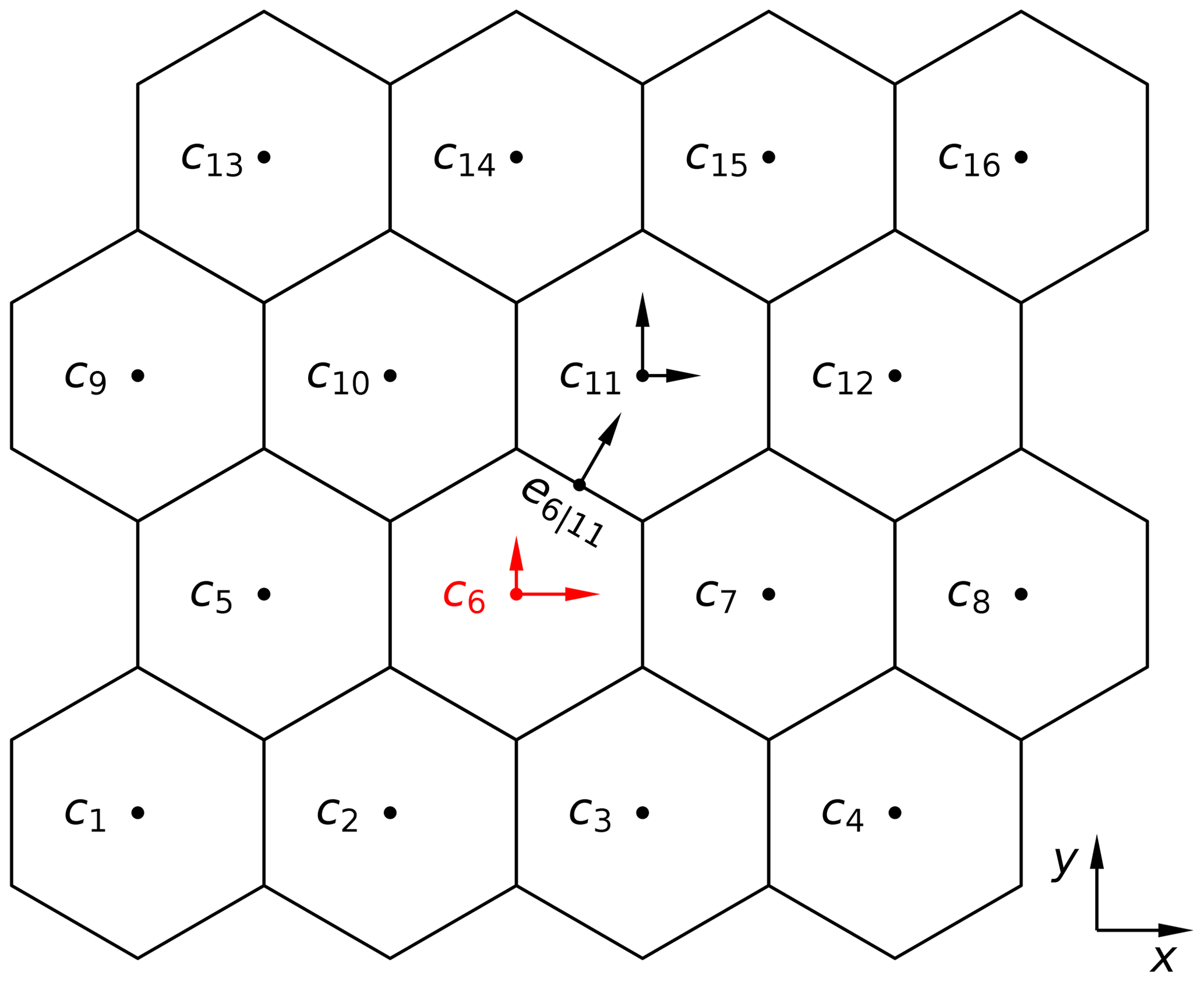
Figure 2 Schematic diagram of coupling MPAS-Ocean with PALM with PALM running only on selected cells. In this example, PALM is running at the center of cell c₆ (in red), whereas KPP is used in all other cells (in black). The normal velocity at the edge e_6|11 is therefore affected by both PALM at c₆ and KPP at c₁₁. See the text for more details.

2.2 PALM on GPU

Time-stepping the PALM instances is the most computationally expensive step in the coupled MPAS-Ocean and PALM system described above. It is therefore sensible to accelerate PALM using GPU. Since there is no need for communications among different instances of the embedded PALM, they may run efficiently on GPUs in parallel on a massive scale. Note that the size of the problem we intend to solve by each embedded PALM instance is small enough to be deployed on one GPU. In fact, a single GPU on modern high-performance computing systems has enough memory to allow multiple PALM instances for our purposes. In addition, each PALM instance is associated with an MPAS-Ocean grid cell in our coupling framework and therefore a single MPI task. For these reasons, we target our porting of PALM on a single GPU without inter-GPU communications.

Significant modification and reduction of the PALM code (version 5.0) were conducted before porting it on GPU. In particular, all the special treatment of complex topography and surface types were removed, along with the atmospheric variables, all of which are irrelevant to our OSBL application here. We also removed the option to use different numerical schemes and hard-coded it to use the fifth- and sixth-order advection scheme of Wicker and Skamarock (2002) and third-order Runge–Kutta time-stepping scheme. We used an external fast Fourier transform library (FFTW) for the pressure solver (an option in PALM) in the CPU version for benchmarking. These steps significantly reduced the amount of effort required to port PALM on GPU.

This customized version of PALM was ported on GPU using OpenACC directive-based parallel programming model (https://www.openacc.org/, last access: 8 April 2021) and the NVIDIA CUDA Fast Fourier Transform library (cuFFT, https://developer.nvidia.com/cufft, last access: 8 April 2021). Porting PALM involved two iterative steps: (1) parallelizing the loops and (2) optimizing data locality. In the first step we wrapped all the loops in the time integration subroutine with the OpenACC “parallel” directive, which allows for automatic parallelization of loops. Some loops, especially in the tridiagonal solver and the turbulence closure subroutines, were restructured to ensure independency. A lower degree of parallelism was employed for loops that cannot be easily restructured to remove the dependency between iterations. This step generally slows down the code because of the large amount of data exchanges occurring between the CPU and the GPU. Therefore, optimizing data locality is required. This was done by enlarging the data regions of the parallelized loops on GPU. Then we moved on to parallelize another segment of the code and iterated between the two steps.

In the process of porting the code, some loops are executed on the CPU and some on the GPU. So extreme caution is required to make sure the data are synchronized between the CPU and the GPU when necessary. Eventually, the data region on GPU is large enough to cover the entire time integration subroutine. This reduces the data exchange between the CPU and the GPU to mostly at the beginning and the end of the time integration, which will occur once per MPAS-Ocean time step. As most of the subroutines during the time integration are ported on GPU, values of the variables are updated on the CPU rather infrequently only when it is necessary. This significantly reduces the time-consuming data exchange between the CPU and the GPU, which leads to overall acceleration of the code. The cuFFT library was used to accelerate the pressure solver in PALM, which uses fast Fourier transform to solve the Poisson equation.

The speedup of porting PALM on GPU was benchmarked by running the standalone PALM with and without GPU on two machines: (1) a Linux workstation with an Intel Xeon Silver 4112 CPU at 2.60 GHz and an NVIDIA Quadro RTX 4000 GPU and (2) the High Performance Computing system at Oak Ridge National Laboratory (Summit) with 2 IBM POWER9 CPUs and 6 NVIDIA Tesla V100 GPUs on each node. For the benchmarking on both machines, only 1 CPU and 1 GPU were used. Figure 3 shows the speedup in total run time and the three most time-consuming subroutines. The speedup factor is defined as the ratio of the run time on 1 CPU divided by the run time on 1 CPU and 1 GPU, all with 1 MPI task. Note that the model throughput per watt of power consumption would be a much better measure of the speedup and the benefit of porting the code on GPU. However, that measure is difficult to obtain. In practice, since we intend to run multiple PALM instances inside MPAS-Ocean, each associated with a single MPAS-Ocean grid cell and therefore 1 MPI task, and since the coupled MPAS-Ocean and PALM as a whole will be running on multiple CPUs and GPUs, the faster each PALM instance runs, the more flexible the parallel layout could be to achieve maximum overall efficiency. Therefore, this measure of speedup in run time is useful.

In general, a 10–16 times speedup was achieved by porting PALM on GPU, especially for relatively large problem sizes for which the full capability of the GPU can be used. For subroutines that have many independent loops, such as the prognostic equations, the speedup can be larger than a factor of 65. However, the overall speedup was strongly limited by the pressure solver in which the Fourier transform restricts the degree of parallelism, especially for smaller problems. Note that this speedup is achieved by a straightforward application of the OpenACC parallel directives to parallelize the loops and copying the data to GPU at the beginning of the time integration. Further speedup is possible by improving the memory management, and fine-tuning the parallelization of loops and data locality to better suit the GPU capability, which are beyond the scope of this study.

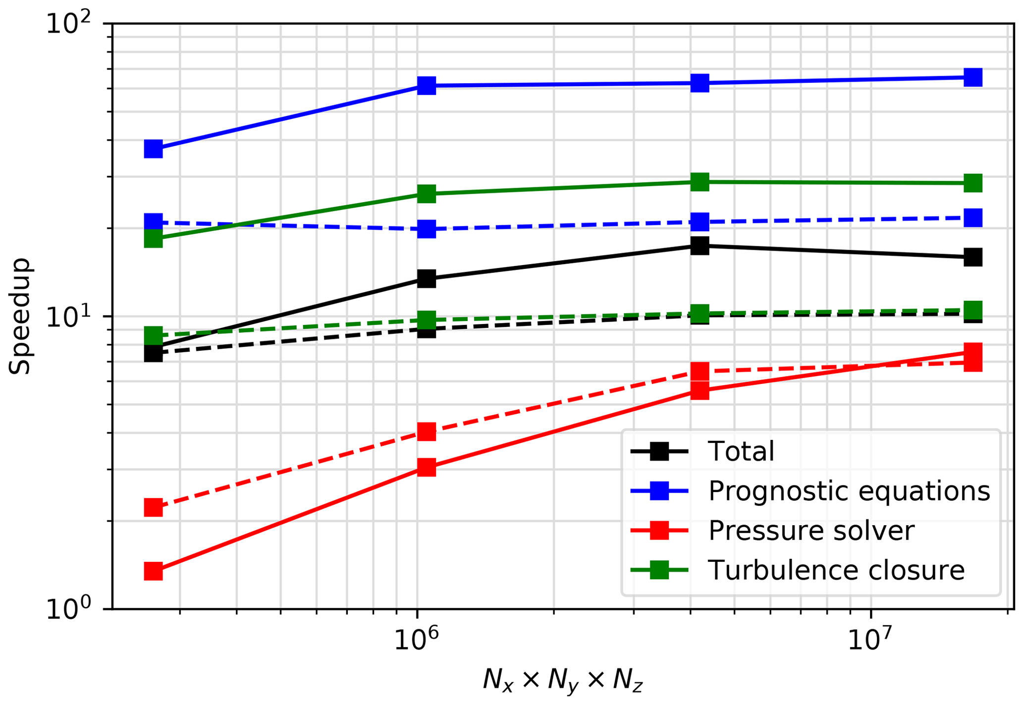
Figure 3 Speedup factor as a function of problem size ($N_x\times N_y\times N_z$). The speedup factor is defined here as the ratio of the run time on 1 CPU divided by the run time on 1 CPU+1 GPU, all with 1 MPI task. The black line shows the speedup in total time and colored lines show the speedup in the three most time-consuming subroutines. Solid lines show the speedup on Summit and dashed lines on the Linux workstation.

3 Evaluation

Here we evaluate the coupled MPAS-Ocean and PALM using two idealized test cases. The first and simplest is in a single-column configuration, which was used throughout the development. The goal of this configuration is a test of one-way coupling from small-scale to large-scale dynamics in Eqs. (1) and (2) by estimating the small-scale forcing terms in Eqs. (9) and (10) from PALM. This also allows a test of the remapping between the vertical grids of MPAS-Ocean and PALM.

The second test case is a simulation of mixed layer eddies in MPAS-Ocean with PALM running on multiple MPAS-Ocean grid cells. The goal of this test case is twofold. First, this case allows us to test the capability of running multiple PALM instances within MPAS-Ocean and distributing the different PALM instances on multiple GPUs. Second, this case provides a way to test the two-way coupling between MPAS-Ocean and PALM under more complex and realistic conditions. In particular, the development of mixed layer eddies in this case introduces spatial heterogeneity and large-scale forcing from advection and lateral mixing, though baroclinic instability in PALM is excluded as a result of missing the lateral gradients.

3.1 Single-column test

MPAS-Ocean allows for a minimum of 16 columns in a “single-column” mode, in which the 16 columns are forced by the same surface forcing and are essentially identical to each other due to the lack of lateral processes. Therefore, ideally running PALM in the single-column MPAS-Ocean is essentially the same as running the standalone PALM as there should be no large-scale forcing terms. In practice, this is true only if PALM is running in all 16 columns. If PALM is only running on one of these columns while KPP is used in other columns, as illustrated in Fig. 2, different solutions between PALM and KPP under the same forcing conditions will result in some spurious large-scale forcing to PALM. This is especially the case for the momentum since the momentum is solved on cell edges in MPAS-Ocean; i.e., it is affected by the momentum fluxes from both the PALM cell and the KPP cells. This 16-cell “single-column” MPAS-Ocean configuration allows us to assess the impact of this issue and explore possible remedies.

The coupled MPAS-Ocean and PALM is tested in this single-column configuration under different idealized forcing scenarios using various combinations of constant wind stress, constant surface cooling, and diurnal solar heating. Here we only present one case in detail as an example. In this case the simulation is initialized from a stable stratification with a surface temperature of 20 ^∘C and a constant vertical gradient of 0.01 ${}^{\circ }\mathrm{C}{\mathrm{m}}^{-\mathrm{1}}$. Salinity is constant at 35 psu to make sure the coupling does not introduce spurious tendencies. We run the MPAS-Ocean simulation from rest for two days with a time step of 30 min. The depth of the simulation domain is 102.4 m, divided into 80 layers with constant layer thickness of 1.28 m. For some configurations we also repeated the same simulation with a coarse vertical resolution of 5.12 m to test the sensitivity to vertical remapping.

The surface forcing is an idealized diurnal heating and cooling with constant wind stress of 0.1 N m⁻². An idealized diurnal cycle of the solar radiation F_s is used,

$$\begin{array}{}\text{(15)}& F_{\mathrm{s}}\left(t\right)=F_{\mathrm{0}}max\left\{\cos \left[\mathrm{2}\mathit{\pi }\left({\displaystyle \frac{t}{\mathrm{86}\mathrm{400}}}-\mathrm{0.5}\right)\right],\mathrm{0}\right\},\end{array}$$

where F₀=500 W m⁻² is the maximum solar radiation at noon and t is the time of a day in seconds. Absorption of solar radiation in the water column is computed using the two-band approximation of Paulson and Simpson (1977) assuming Jerlov water type IB. A constant surface cooling of −159.15 W m⁻² is applied at the surface, balancing the solar heating when integrated over a day. The Coriolis parameter is set to $\mathrm{1.028}\times {\mathrm{10}}^{-\mathrm{4}}$ s⁻¹, equivalent to the value at a latitude of 45^∘ N. This test case yields an inertial oscillation in the velocities with a period of about 17 h in addition to the diurnal heating and cooling.

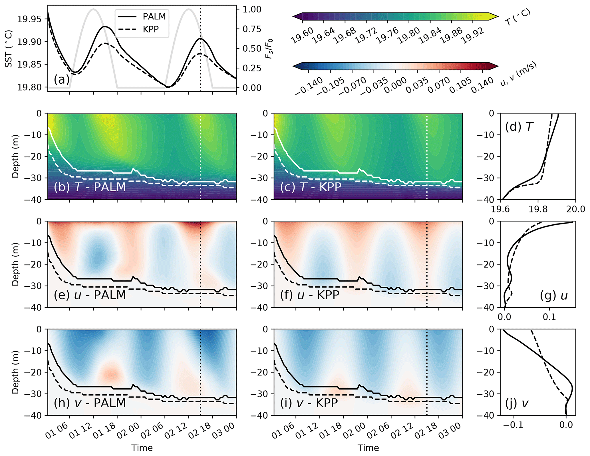
Figure 4 A comparison between KPP and standalone PALM simulations in the diurnal heating case. Panel (a) shows the simulated sea surface temperature (SST, ^∘C) in standalone PALM (solid line in black) and KPP (dashed line). For reference the diurnal factor ($F_{\mathrm{s}}/F_{\mathrm{0}}$) in Eq. (15) is also shown (gray line, vertical axis on the right). Panels (b), (c), (e), (f), (h), and (i) show the simulated temperature (T, ^∘C) and velocities (u, v, m s⁻¹) in x and y directions, respectively, in PALM and KPP. Solid and dashed lines mark the boundary layer base in PALM and KPP, respectively, defined as the depth where the stratification reaches its maximum. The dotted line in these panels marks the time when the profiles in PALM and KPP are compared in (d), (g), and (j), respectively.

The coupled MPAS-Ocean and PALM is tested by running PALM only at the sixth cell c₆ (see Fig. 2). All other 15 cells use KPP for the vertical mixing with a typical configuration (Van Roekel et al., 2018). PALM runs on a $\mathrm{160}\mathrm{m}\times \mathrm{160}\mathrm{m}\times \mathrm{80}\mathrm{m}$ domain with $\mathrm{128}\times \mathrm{128}\times \mathrm{80}$ grid cells, yielding a resolution of $[\mathrm{d}x,\mathrm{d}y,\mathrm{d}z]=[\mathrm{1.25},\mathrm{1.25},\mathrm{1}]$ m. This configuration of PALM is enough to give statistically robust mean vertical profiles of the fluxes that are exchanged with MPAS-Ocean. PALM starts with some small random perturbations on the temperature and velocity fields (between depths of around 4 and 28 m) during the first 150 s and then runs for 1 h to allow the turbulence to develop before the initial step of MPAS-Ocean. Then the mean fields of PALM are forced back to the initial profiles of MPAS-Ocean described above, while keeping the turbulent perturbations developed in the PALM initial step,

$$\begin{array}{}\text{(16)}& {\mathit{\varphi }}^{\mathrm{f}*}(x,y,z)={\mathit{\varphi }}^{\mathrm{f}}(x,y,z)-\stackrel{\mathrm{‾}}{{\mathit{\varphi }}^{\mathrm{f}}}\left(z\right)+{\mathit{\varphi }}^{\mathrm{c}}\left(z\right),\end{array}$$

where ϕ^f* is the updated PALM field, ϕ^f is the original, $\stackrel{\mathrm{‾}}{{\mathit{\varphi }}^{\mathrm{f}}}$ is the horizontal average over the PALM domain, and ϕ^c is the initial condition from MPAS-Ocean (see Fig. 1).

We first compare the solutions of this test case in standalone PALM and KPP in Fig. 4. It is clearly seen that in this test case KPP gives quite different solutions than the standalone PALM. In particular, KPP yields slightly stronger vertical mixing indicated by the deeper boundary layer by a few meters. As a result, the simulated temperature is cooler throughout most parts and warmer near the base of the boundary layer (panel d), and the maximum sea surface temperature (SST) during a diurnal cycle is about 0.04 ^∘C cooler (panel a) in KPP than in PALM. The simulated velocities are clearly affected by the diurnal heating during different phases of the inertial oscillation in PALM, but not in KPP.

For the coupled MPAS-Ocean and PALM, with the small-scale forcing Eqs. (9) and (10) from PALM applied to all 16 cells, we expect the results to be identical to the standalone PALM, except perhaps for some small differences due to the differences in time stepping. This is indeed the case, as shown by comparing the blue line and black line in Fig. 5. Here the profiles in Fig. 5 are taken at the time of SST maximum indicated by the dotted line in Fig. 4.

Since the small-scale forcing of tracers in Eq. (10) is directly applied to the tracer equations at the MPAS-Ocean cell centers, the coupling of tracers (here temperature) is straightforward even though PALM is running on one cell c₆ (Fig. 2) as there is no direct impact from neighboring cells. This can be seen from the agreement of the dark red line and the black line in Fig. 5a, in which ${\mathit{\tau }}_{\text{LS}}^{\mathit{u}}=\mathrm{\infty }$ or equivalently ${\mathit{F}}_{\text{LS}}^{\mathit{u}}=\mathrm{0}$ following Eq. (11) effectively cuts off the influence of neighboring KPP cells on the momentum equations in PALM. However, as the momentum at the center of the PALM cell (c₆) is directly coupled with the neighboring KPP cells (by solving only the normal velocity at edges), we see some differences as the coupling of the momentum gets tighter with a shorter relaxation timescale for the momentum (see the transition from dark red to light red in Fig. 5). In particular, although the momentum profiles appear to be slightly closer to the standalone PALM as the relaxing is stronger, the temperature starts to be affected by this strong coupling with neighboring cells. The surface temperature (upper 10 m) gets warmer due to the diurnal heating and the layer immediately below gets slightly cooler as compared to the standalone PALM. This is probably an artifact due to the mismatching tendencies of warmer surface temperature from PALM and weaker velocity shear from KPP, making the surface layer in the embedded PALM more stable. The momentum near the base of the boundary layer is also strongly influence by neighboring cells running KPP. Similar behavior is also seen in a purely shear-driven entrainment case (not shown).

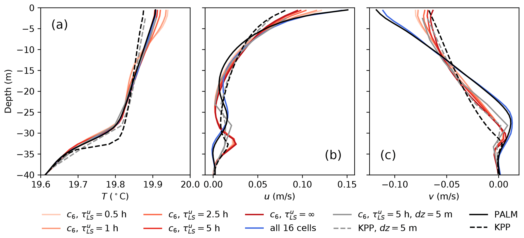
Figure 5 A comparison of the temperature (a), zonal velocity (b), and meridional velocity (c) profiles with different configurations and coupling strategies. The profiles are taken at the SST maximum (about 3 h after the solar radiation maximum) during the second diurnal cycle of the diurnal heating cases (dotted line in Fig. 4). On top of the profiles in the standalone PALM (black solid) and KPP (black dashed) from panels d, g, and j of Fig. 4, we overlay the profiles from a set of sensitivity tests with different configurations and coupling strategies. Light to dark red lines show the results of simulations with different momentum relaxing timescales from ${\mathit{\tau }}_{\text{LS}}^{\mathit{u}}=\mathrm{0.5}$ h to zero momentum relaxing (${\mathit{\tau }}_{\text{LS}}^{\mathit{u}}=\mathrm{\infty }$). The blue line shows the results of a simulation in which the tendencies of PALM are applied to all 16 cells, versus only cell c₆ in other cases. Gray solid and dashed lines show the same as the c₆, ${\mathit{\tau }}_{\text{LS}}^{\mathit{u}}=\mathrm{5}$ h case and the KPP case, respectively, but with MPAS-Ocean running on a coarse resolution of dz=5.12 m. In all cases (when applicable) the relaxing timescale for tracers is ${\mathit{\tau }}_{\text{LS}}^{\mathit{\theta }}=\mathrm{0.5}$ h.

The similar results between the coarse vertical resolution (gray line) and the fine vertical resolution (red line) in Fig. 5a suggest that embedding a high-fidelity LES is able to improve the temperature distribution of a coarse-vertical-resolution parent model, and the error of vertical remapping with the piecewise quartic method (White and Adcroft, 2008) is minimal. However, embedding a fine-vertical-resolution KPP does not help, indicated by the similar results of black and gray dashed lines in Fig. 5a (in this case the coarse resolution KPP appears to perform better near the boundary layer base; see also Van Roekel et al., 2018). Some improvements over KPP in the simulated momentum are also seen in both the fine-vertical-resolution case (red solid lines in Fig. 5b and c) and the coarse-vertical-resolution case (gray solid lines in Fig. 5b and c). But since the momentum at the cell center is reconstructed from the normal velocities at all edges of a cell, which are strongly influenced by the neighboring KPP cells, its profiles resemble more the momentum profiles in KPP than that in PALM.

Spatial influence of running PALM on the cell center of a single cell in the 16-cell single-column configuration is shown in Fig. 6. The difference between all the 15 KPP cells and the PALM cell (marked by the plus sign) for temperature is roughly uniform, except the two adjacent cells on the left and right, and the cell at the upper right (panel a, note that the domain is doubly periodic), likely due to the feedback from changes in the velocity in those cells (panels b and c). The changes in zonal and meridional velocities are results of the interpolation of small-scale forcing terms from cell center to cell edges, and the reconstruction of the zonal and meridional velocities from normal velocities at edges. Note that the surface fluxes are consistent across all cells and applied directly as boundary conditions. So there is no feedback from the different simulated surface temperature and velocity between PALM and KPP cells.

Figure 6 Distribution of the differences in temperature (a), zonal velocity (b), and meridional velocity (c) at the surface between the KPP cells and the PALM cell (marked by “+”) in the single-column test. Here the relaxing timescale for the momentum and tracers are ${\mathit{\tau }}_{\text{LS}}^{\mathit{u}}=\mathrm{5}$ h and ${\mathit{\tau }}_{\text{LS}}^{\mathit{\theta }}=\mathrm{0.5}$ h.

Note that running PALM on the cell edges of MPAS-Ocean (e.g., on e_6|11 in Fig. 2) would not help to eliminate this issue in the coupling of the momentum. At first thought it might appear promising as in that case the normal velocity at the edge can be directly used to update the momentum in PALM. However, since the tangential velocity in MPAS-Ocean (Ringler et al., 2010) is diagnosed from the normal velocity at all the edges of the two neighboring cells (e.g., c₆ and c₁₁) of an edge (e.g., e_6|11), the influence of neighboring KPP cells is still there. We therefore choose to run PALM on the MPAS-Ocean cell centers and use a relatively long (5 h) relaxing timescale for the momentum to alleviate the coupling issue, while acknowledging that this issue deserves further investigation.

3.2 Mixed layer eddy test

The setup of the mixed layer eddy test case is guided by similar simulations in both GCMs (Fox-Kemper et al., 2008) and LES models (Hamlington et al., 2014). However, since our focus is not on the mixed layer eddy itself, we are not comparing the simulation results here with those in the literature. Instead we focus on the coupling between MPAS-Ocean and PALM in the presence of some mixed layer eddies.

Here we run MPAS-Ocean with a two-front, or warm filament, setup on a domain of $\mathrm{72}\mathrm{km}\times \mathrm{62.4}\mathrm{km}\times \mathrm{150}\mathrm{m}$ with 14 400 cells and 50 vertical levels, corresponding to horizontal (distance between cell centers) and vertical grid sizes of 600 m and 3 m, respectively. The initial temperature field T₀ is uniformly distributed in the x direction with two fronts in the y direction,

$$\begin{array}{}\text{(17)}& {\displaystyle }\begin{array}{rl}{T}_{\mathrm{0}}(y,z)=& T_{\mathrm{b}}+{\displaystyle \frac{N^{\mathrm{2}}}{{\mathit{\alpha }}_{\mathrm{T}}g}}(z+H)\\ & +{\displaystyle \frac{L_{\mathrm{f}}{M}_{\mathrm{f}}^{\mathrm{2}}}{\mathrm{2}{\mathit{\alpha }}_{\mathrm{T}}g}}\mathit{\{}\mathrm{1}+\tanh \left[{\displaystyle \frac{\mathrm{2}(y-y_{\mathrm{1}})}{L_{\mathrm{f}}}}\right]\\ & -\tanh \left[{\displaystyle \frac{\mathrm{2}(y-y_{\mathrm{2}})}{L_{\mathrm{f}}}}\right]\mathit{\}},\end{array}\text{(18)}& {\displaystyle }{N}^{\mathrm{2}}=\left\{\begin{array}{ll}{N}_{\text{ml}}^{\mathrm{2}},& \text{if}z>-H,\\ N_{\text{int}}^{\mathrm{2}},& \text{if}z\le -H,\end{array}\right.\end{array}$$

where T_b=16 ^∘C is the temperature at the base of the mixed layer, H=50 m is the mixed layer depth, and $N_{\text{ml}}^{\mathrm{2}}=\mathrm{1.96}\times {\mathrm{10}}^{-\mathrm{7}}$ s⁻² is the stratification within the mixed layer and $N_{\text{int}}^{\mathrm{2}}=\mathrm{1.96}\times {\mathrm{10}}^{-\mathrm{5}}$ s⁻² below, corresponding to ${\partial }_{z}T={\mathrm{10}}^{-\mathrm{4}}$ ${}^{\circ }\mathrm{C}{\mathrm{m}}^{-\mathrm{1}}$ and ${\partial }_{z}T={\mathrm{10}}^{-\mathrm{2}}$ ${}^{\circ }\mathrm{C}{\mathrm{m}}^{-\mathrm{1}}$, respectively, using a linear equation of state with the thermal expansion coefficient ${\mathit{\alpha }}_T=\mathrm{2}\times {\mathrm{10}}^{-\mathrm{4}}$ ${}^{\circ }{\mathrm{C}}^{-\mathrm{1}}$ and the gravity g=9.81 m s⁻². The front width is L_f=10 km, with the horizontal buoyancy gradient $M_{\mathrm{f}}^{\mathrm{2}}=\mathrm{3.92}\times {\mathrm{10}}^{-\mathrm{8}}$ s⁻² (${\partial }_{y}T=\mathrm{2}\times {\mathrm{10}}^{-\mathrm{5}}$ ${}^{\circ }\mathrm{C}{\mathrm{m}}^{-\mathrm{1}}$). The initial front locations are y₁=15.6 km and y₂=46.8 km. The salinity is constant at 35 psu. The Coriolis parameter is $f={\mathrm{10}}^{-\mathrm{4}}$ s⁻¹. These parameters correspond to a Richardson number $\mathit{\text{Ri}}=N_{\text{ml}}^{\mathrm{2}}{f}^{\mathrm{2}}/M_{\mathrm{f}}^{\mathrm{4}}=\mathrm{1.28}$ in the frontal regions. The two fronts are initialized from rest (unbalanced with the horizontal temperature gradients) with small perturbations on the temperature fields to promote the development of mixed layer instability. The surface is forced by constant wind stress of 0.1 N m⁻² in the x direction. Since the MPAS-Ocean simulation domain is doubly periodic in the horizontal, the two fronts move to the right of the wind direction due to Ekman transport. The result is a stable front in which warmer surface water moves over on top of the cold water and an unstable front in which both the Ekman-driven convective instability and baroclinic instability occur.

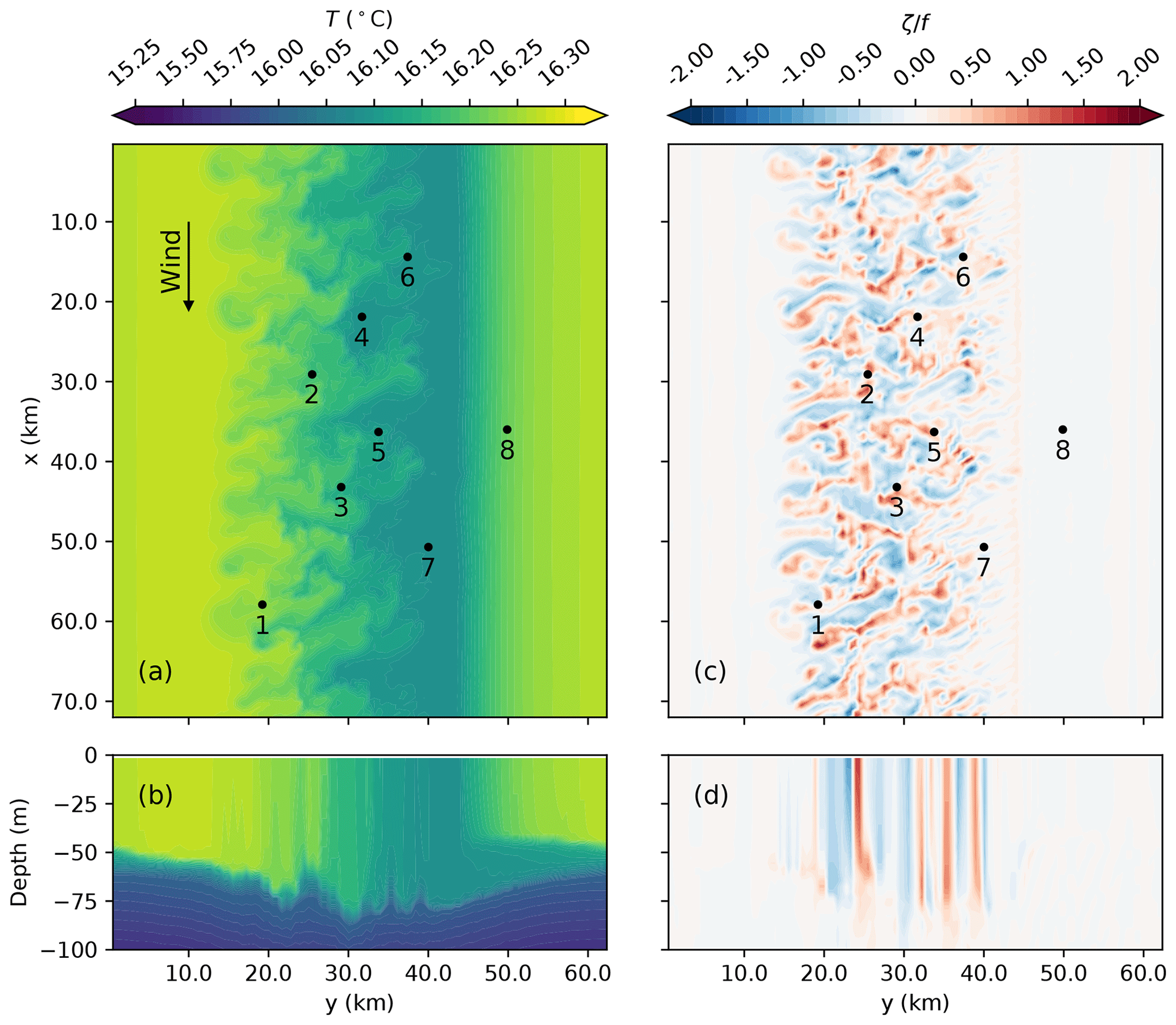
Figure 7 Horizontal (a, c) and vertical (b, d) snapshots of the temperature (a, b; T in ^∘C) and relative vorticity normalized by the Coriolis parameter (c, d; $\mathit{\zeta }/f$) at the beginning of day 16 in the mixed layer eddy case. The location of each of the MPAS-Ocean cells running PALM is marked by a black dot and assigned a number for quick reference. The wind is in the x direction as shown by the arrow, with a constant wind stress of 0.1 N m⁻². Note that the contour lines for temperature have an interval of 0.05 ^∘C below 16 ^∘C and 0.01 ^∘C above to highlight the eddy structures in the mixed layer.

The MPAS-Ocean simulation is first spun up with KPP for 15 d with a time step of 5 min, allowing the mixed layer eddies to develop. Then starting from day 16, three branch runs of 30 h are conducted, which are the focus of the analysis here. The first run continues to use KPP in all the cells. The second run uses PALM at 8 selected cells and KPP elsewhere, with a PALM domain of $\mathrm{160}\mathrm{m}\times \mathrm{160}\mathrm{m}\times \mathrm{120}\mathrm{m}$ and $\mathrm{128}\times \mathrm{128}\times \mathrm{120}$ grid cells, and the same coupling strategy as in the single-column test using relaxing timescales of ${\mathit{\tau }}_{\text{LS}}^{\mathit{\theta }}=\mathrm{0.5}$ h and ${\mathit{\tau }}_{\text{LS}}^{\mathit{u}}=\mathrm{5}$ h. The third run is the same as the second (i.e., same initial condition, surface forcing, and PALM cells), except there is no coupling between MPAS-Ocean and PALM (i.e., no exchange of large-scale and small-scale forcings). Comparing the former two runs shows the different responses in KPP and PALM to the same surface wind forcing and large-scale forcing due to mixed layer eddies, whereas comparing the latter two shows the impact of the large-scale forcing on the small-scale turbulence in PALM.

Figure 7 shows a snapshot of the temperature and relative vorticity fields at the beginning of day 16. Note that the unstable front initially at y=46.8 km has moved to around y=25 km, whereas the stable front initially at y=15.6 km has moved to around y=45 km (out and re-entering the domain) due to the Ekman transport towards the negative y direction and the doubly periodic domain. The locations of the eight MPAS-Ocean cells running PALM are marked and labeled for quick reference. For brevity, here we only present the results of four representative cells: cells 1 and 3 located at both sides of the unstable front, where active mixed layer eddies are developing, and cell 7 and 8 located at both sides of the stable front, with the latter strongly affected by the Ekman advection of surface warm water.

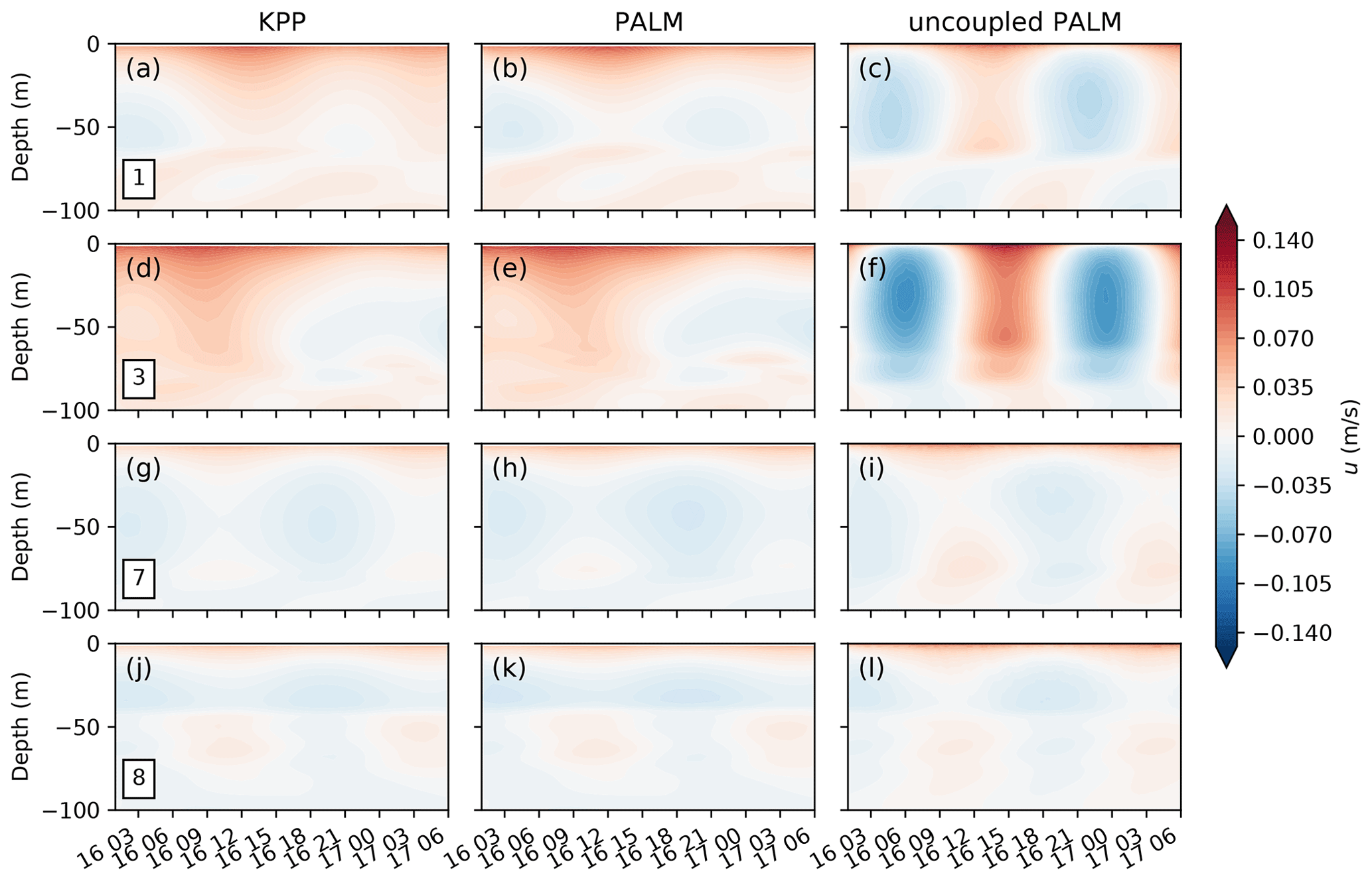
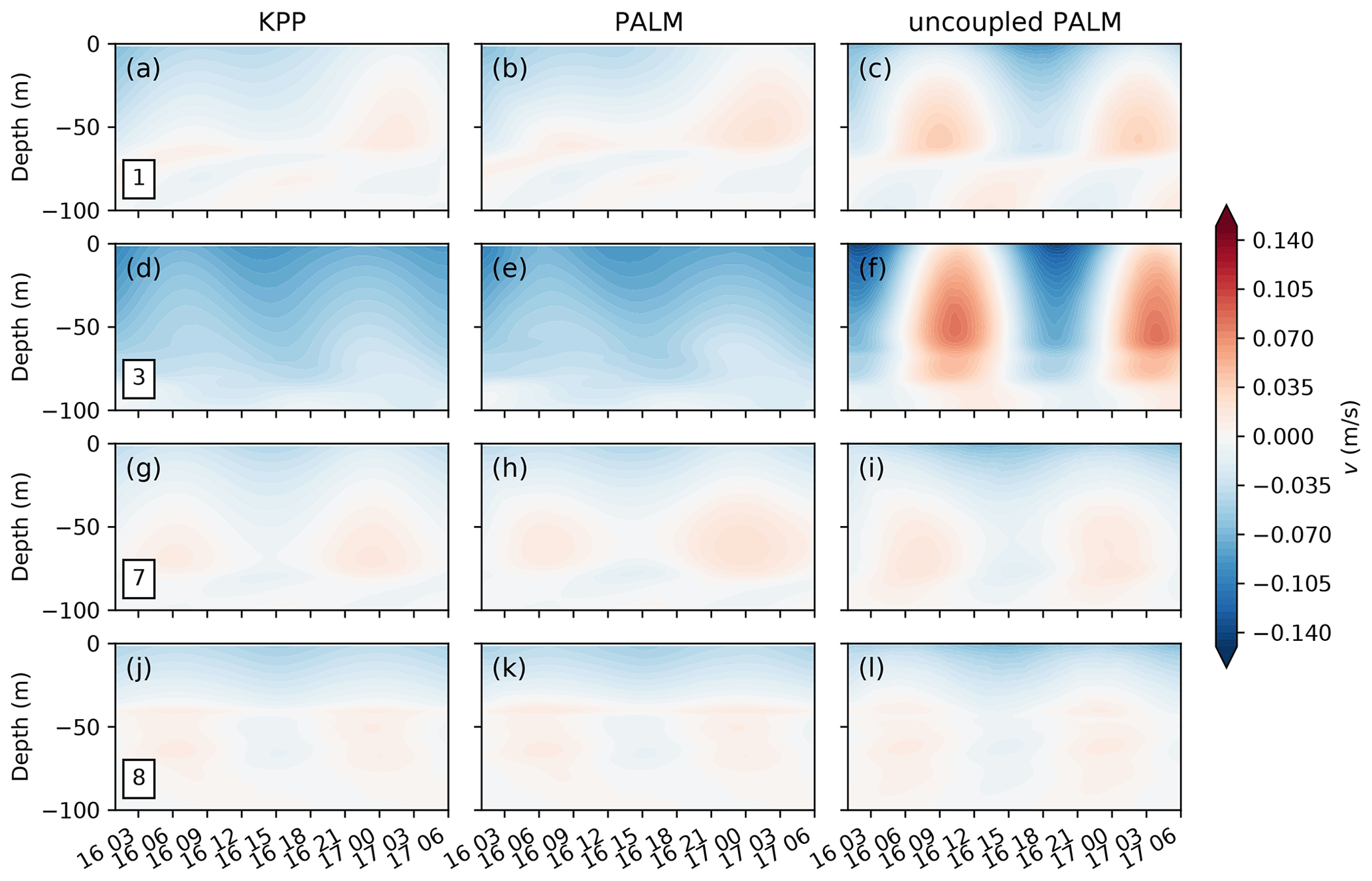
Figures 8–10 show the time evolution of the temperature and the zonal and meridional velocities at four locations. It is clearly seen that at cells 1 and 3, both the temperature and momentum are strongly affected by the large-scale forcing due to the mixed layer eddies (panels a, b, d and e in all three figures), where otherwise under constant surface wind forcing and rotation would develop strong inertial oscillation with a period of about 17 h (panels c and f in Fig. 9 and 10). The similarity between KPP and PALM at these two locations suggests the dominance of large-scale forcing due to mixed layer eddies in the evolution of temperature and momentum, while small differences are still noticeable suggesting the potential importance of boundary layer turbulence in feeding back to the evolution of mixed layer eddies. At cell 7, the large-scale forcing is relatively small in the absence of active mixed layer eddies and Ekman advection of surface warm water. Therefore, the temperature and momentum are similar to the uncoupled PALM simulations (panels g, h and i of all three figures). At cell 8, a second shallower mixed layer is developed and getting warmer and warmer as a result of the Ekman advection of surface warm water. The temperature is strongly affected by this large-scale forcing (Fig. 8j–l), whereas the momentum is relatively less affected (panels  j–l of Figs. 9 and 10).

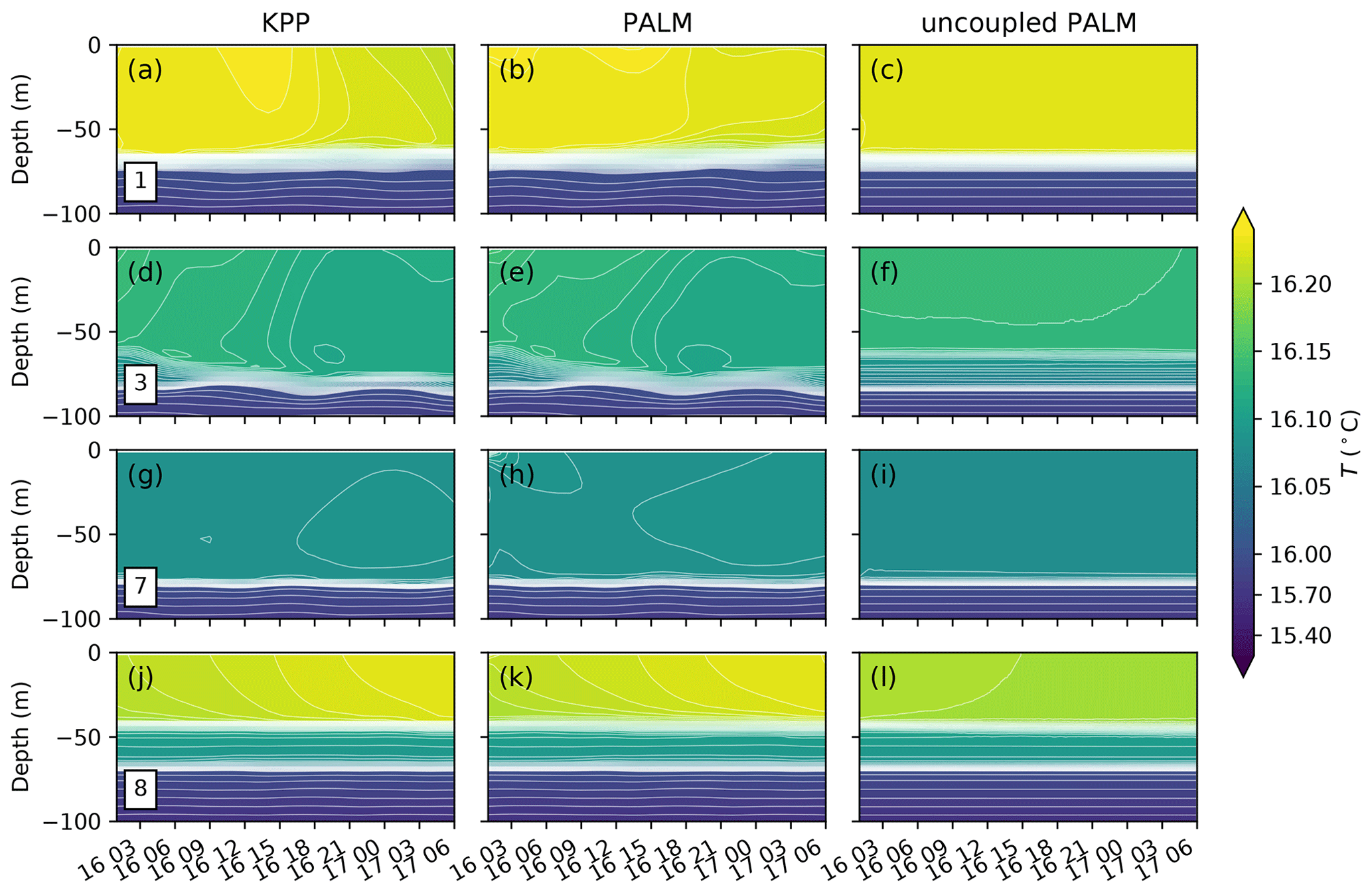
Figure 8 Evolution of temperature profiles at the cells 1, 3, 7, and 8 labeled in Fig. 7. Three columns of panels show the profiles in the MPAS-Ocean simulations with KPP (a, d, g, j) and PALM (b, e, h, k), and the profiles in the uncoupled PALM (c, f, i, l). Note that the contour lines for the temperature have an interval of 0.05 ^∘C below 16 ^∘C and 0.005 ^∘C above to highlight the structures in the mixed layer.

Figure 9 Same as Fig. 8, but for the zonal velocity.

Figure 10 Same as Fig. 8, but for the meridional velocity.

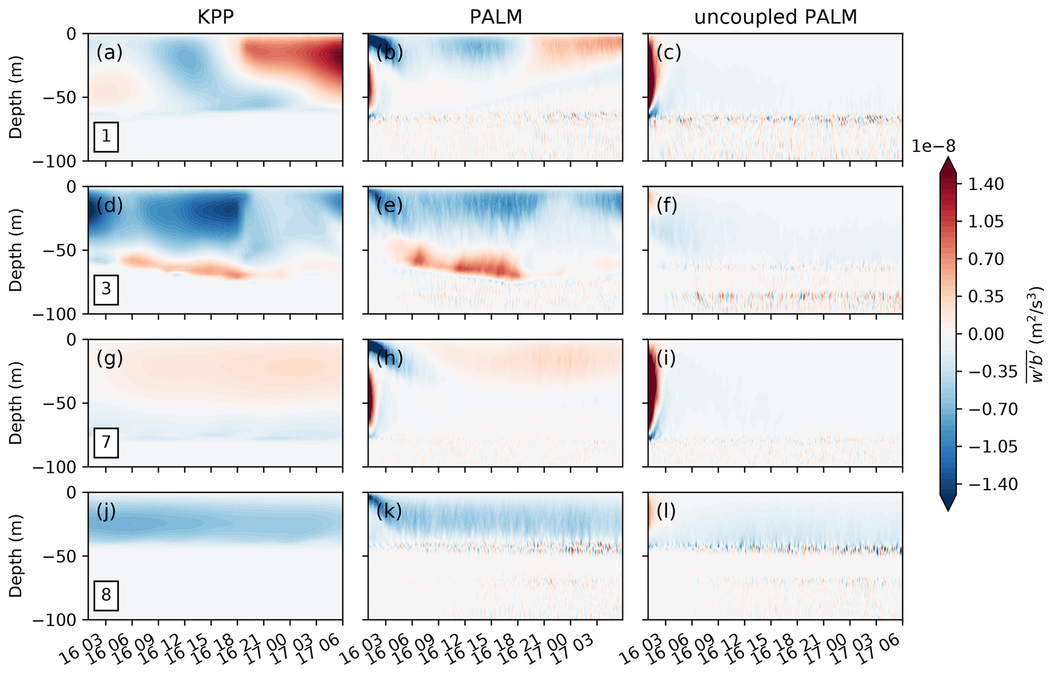
Finally, we demonstrate the influence of large-scale forcing on the small-scale turbulence statistics by showing the time evolution of the vertical buoyancy flux profile in the three runs in Fig. 11. The buoyancy flux in the KPP run (left panels) is diagnosed from the MPAS-Ocean output of the stratification, the vertical turbulent diffusivity and the non-local fluxes (zero in this case). The results in the coupled and uncoupled PALM runs (middle and right panels) are the sum of the resolved and subgrid-scale buoyancy fluxes in PALM. Consistent with Figs. 8–10, the vertical buoyancy flux is strongly affected by the large-scale forcing due to mixed layer eddies and Ekman-driven convection at cells 1 and 3, but less so at cells 7 and 8. Though qualitatively similar, the vertical buoyancy fluxes in response to the large-scale forcing of mixed layer eddies are quantitatively different between MPAS-Ocean runs with KPP and with PALM, suggesting the potential importance of a better representation of boundary layer turbulence in simulating the mixed layer eddies.

Traditionally an OSBL parameterization is often tuned against some forced LES without large-scale forcing, as in the uncoupled PALM case (c, f, i, and l of Figs. 8–11), whereas a mixed layer eddy parameterization is tuned using GCMs with some OSBL parameterization, as in the KPP case (a, d, g, and j). The results here suggest that we might need to explicitly consider the influence of the mixed layer eddies on the OSBL turbulence and vice versa when tuning the parameterizations. The coupled MPAS-Ocean and PALM provides a way to do this. It should be noted that here we are showing the differences, rather than quantifying the errors, between the runs with and without the coupling across scales. The latter would require a careful evaluation against an LES simulation of the interactions between mixed layer eddies and the OSBL turbulence (e.g., Hamlington et al., 2014). We are also missing the effect of the large-scale lateral gradients on the dynamics of the small-scale turbulence in this test case, which will be discussed in Sect. 4.1.

Figure 11 Same as Fig. 8, but for the vertical buoyancy flux. Unlike Fig. 8, the middle panels are directly from the PALM output. The large values at the beginning of the simulation for (b), (c), (h), and (i), for example, are due to the spin-up of the turbulence in PALM.

4 Discussion

Traditionally, the primary goal of embedding a fine-resolution process-resolving model inside a coarse-resolution GCM is to improve the skill of the coarse-resolution GCMs by improving the representation of small-scale processes. Alternatively, here we show that embedding a high-fidelity, three-dimensional LES in GCMs also provides a promising framework to systematically conduct process studies of turbulent mixing in the OSBL in the context of larger-scale processes, such as submesoscale eddies and fronts. In the traditional case, the focus is on the large-scale GCMs so that the embedded fine-resolution model does not have to be accurate on its own merits, i.e., we only need to represent the most important effects of the small-scale processes on large scales. This opens the door for various choices of the embedded small-scale model with reduced dimension or reduced physics, such as stochastic models (e.g., Grooms and Majda, 2013) or machine learning models (e.g., Brenowitz and Bretherton, 2018; O'Gorman and Dwyer, 2018). In our case, however, the interests are also on the small-scale processes. Therefore, a process-resolving model with high fidelity such as an LES is necessary.

Given that direct measurements of turbulent mixing in the ocean is sparse, recent development and tuning of new OSBL vertical mixing schemes for GCMs rely heavily on forced LES under a variety of different forcing conditions (e.g., Harcourt, 2013, 2015; Li and Fox-Kemper, 2017; Reichl and Li, 2019). Such LES is often idealized without the influences of large-scale processes, assuming that such influences are additive that can be accounted for by other parameterizations in GCMs. As the horizontal resolution of a GCM becomes finer and finer, such assumption may no longer be valid, especially for an OSBL scheme in which the boundary layer depth is derived from a prognostic equation, such as the OSMOSIS schemes (Damerell et al., 2020). The approach described here may benefit the development of new OSBL schemes by providing an efficient way to generate LES data with the influence of large-scale processes for tuning of the parameters.

One advantage of applying the coupled MPAS-Ocean and PALM to focused process studies, as compared to the forced LES approach, is that the small-scale LES is essentially coupled, though rather loosely, with the large-scale GCM. The effects of large-scale processes, such as advection and lateral mixing, are naturally accounted for at different levels of completeness depending on the flexible coupling strategy. We can use different coupling strategies to study the interactions between the large-scale processes and the small-scale turbulent mixing. Additionally, this approach is also much more computationally efficient as compared to an LES on a large domain to resolve all the important processes, which is often required to study the coupling across scales (e.g., Hamlington et al., 2014; Sullivan and McWilliams, 2019).

4.1 Remaining issues

The coupling between MPAS-Ocean and PALM presented in Sect. 2.1 currently excludes the effect of a lateral gradient of large-scale quantities. Large-scale lateral gradients are needed in the small-scale dynamics to allow processes like baroclinic instability (e.g., Bachman and Taylor, 2016) and are essential for the energy transfer from the large scale to the small scale. In the superparameterization literature, as well as the conventional OSBL parameterization literature, it is often assumed that there is a scale separation between the large-scale processes simulated by the GCMs and the small-scale turbulent processes simulated by the embedded process-resolving model or represented by the parameterization schemes. As the horizontal resolution of the GCMs increases, and the scales of the resolved processes and the small-scale turbulent processes therefore get closer, this assumption may start to break. The multiscale modeling approach presented here can be extended to incorporate such effects by allowing the large-scale forcing terms in Eqs. (4) and (6). A similar approach has been suggested in, for example, Grooms and Julien (2018) for multiscale modeling, as well as applied in LES studies of the frontal regions (e.g., Bachman and Taylor, 2016; Fan et al., 2018). The tricky part is estimating the lateral gradient of large-scale quantities, which strongly depends on the horizontal resolution of the GCMs. Therefore, great caution has to be exercised when interpreting the resolved lateral gradients in the coarse-resolution GCMs.

Even with the GPU-acceleration technique, running PALM in MPAS-Ocean is still computationally intensive. In the present setup in the single-column test (running PALM on one cell while using KPP in others), the total run time on one CPU and one GPU is a few hundreds times longer than using KPP in all cells. In the mixed layer eddy test case, running PALM on 8 cells increases the total run time by over 40 times on 16 CPUs and 8 GPUs. While the computational cost is well justified for applications on studying the small-scale turbulent mixing, for applications on improving the GCM performance, a superparameterization-like approach with high-fidelity and three-dimensional LES embedded in every grid cell in a GCM is still far from practical.

4.2 Moving forward

We have tested the coupled MPAS-Ocean and PALM using some very idealized test cases. The goals of these test cases are to verify the functionality of the coupled system, which provides the foundation for future extensions and applications to more realistic setups. Here we outline a few possible use scenarios that will take advantage of the development in this study.

As mentioned in the previous section, one obvious step forward is to include the effects of large-scale lateral gradients in the embedded PALM. To overcome the limitation of a doubly periodic domain in PALM, one can assume constant background fields with large-scale gradients (${\mathrm{\nabla }}_{\mathrm{h}}^{\mathrm{c}}({)}^{\mathrm{c}}$ terms in Eqs. (13) and (14)), which are updated every coupling period, and adapt Eqs. (4) and (6) to solve for the perturbations around the background fields, to which periodic boundary conditions can be applied. A similar technique has already been used in LES studies of turbulent mixing in an idealized frontal zone assuming that the background buoyancy gradient and velocity shear are in thermal wind balance (e.g., Bachman and Taylor, 2016). This allows the development of baroclinic instability in the embedded LES and a direct comparison with an LES on a larger domain to study the turbulent mixing in the presence of large-scale features such as submesoscale fronts and filaments (e.g., Hamlington et al., 2014; Sullivan and McWilliams, 2019). In addition to significantly reducing the computational cost as compared to an LES on a large domain, the coupled MPAS-Ocean and PALM also allows one to separate the contributions of lateral processes and vertical mixing at different scales by combining different domain sizes, resolutions, and coupling strategies for the large-scale and small-scale dynamics. Of course in doing so a horizontal scale separation is assumed and certain feedback from the small scales to the large scales is lost. One step further to address this is to include the lateral fluxes from the small-scale LES to the large-scale GCM in Eqs. (1) and (2).

With the capability of MPAS-Ocean to use regionally refined mesh, it is possible to set up simulations for focused process studies with high resolution in the study region and low resolution in the surrounding regions. This strategy has already been adopted to conduct global MPAS-Ocean simulations with refined resolution on the US coast and regional simulations with a focus on estuaries (personal communication). The coupling with PALM can further extend the refined study region in an MPAS-Ocean simulation to include non-hydrostatic dynamics. In such applications one can choose to embed PALM inside the finest grid cells of MPAS-Ocean in the focused regions, where the domain size of PALM can be similar to the grid cell size of MPAS-Ocean. In this way, it is reasonable to pass the large-scale gradients estimated in the MPAS-Ocean directly to PALM to allow the development of baroclinic instability and other processes in PALM as discussed above. It would also be interesting to study the impact of turbulent mixing transitioning from an estuary environment to an open ocean environment using this coupled system. This is critical for a seamless coastal to global simulation that MPAS-Ocean is targeted at.

Another application is a systematic exploration of the OSBL turbulent mixing using LES under regional and global forcing conditions with and without the large-scale forcing. One example is LES studies of Langmuir turbulence under hurricane conditions at different phases and locations (e.g., Reichl et al., 2016; Wang et al., 2018). Such studies are traditionally conducted by setting up a set of LESs forced by different conditions from a preexisting larger hurricane simulation. The coupled MPAS-Ocean and PALM will enable simultaneous simulations of the hurricane in MPAS-Ocean and turbulent mixing in PALM, thereby allowing an assessment of the effects of lateral adjustment versus surface forcing during a hurricane. Such a setup also provides useful datasets to assist the development of ocean turbulent mixing parameterizations in these scenarios.

Taking advantage of the flexibility of running PALM only on selected locations in MPAS-Ocean, one may also explore the possibility of improving the simulation results of a GCM by having high-fidelity representations of the turbulent mixing at only a few locations, perhaps borrowing ideas from the data assimilation literature. The high-fidelity representations of the turbulent mixing can be easily drawn from the coupled LES as shown here. Results of such exploration may also be relevant to incorporating direct measurements of OSBL turbulent mixing at various platforms such as research vessels and ocean stations into GCMs.

5 Conclusions

In this paper we have outlined the steps and the progress towards a multiscale modeling approach of studying the ocean surface turbulent mixing by coupling MPAS-Ocean with PALM, following some ideas of the superparameterization approach. However, in contrast to the traditional superparameterization approach which seeks a way to replace the conventional parameterizations, the goal here is to build a flexible framework to better understand the interactions among different processes in the OSBL, thereby providing a pathway to improve the OSBL turbulent mixing parameterizations. For this reason, a high-fidelity and three-dimensional LES is used instead of a simplified model with reduced physics and/or reduced dimensions.

To alleviate the computational burden of embedding PALM in MPAS-Ocean, we ported a customized version of PALM on GPU using OpenACC and achieved an overall speedup of 10–16. Although further speedup is possible, the relatively high computational demand of this high-fidelity and three-dimensional LES still prevents a superparameterization-like approach, with PALM running on every grid cell of MPAS-Ocean, from being practical for long simulations.

However, the flexibility of running PALM only on selected grid cells of MPAS-Ocean, combined with the capability of MPAS-Ocean using an unstructured grid, provides a promising pathway to move forward in simulating the ocean surface turbulent mixing in a multiscale modeling approach. Here we have demonstrated the functionality and potential of this multiscale modeling approach using very simple test cases. As discussed in the previous section, direct progress can be made on various applications of this approach, from a regionally focused process study of the OSBL turbulence in the presence of large-scale phenomena to a systematic exploration of better representations of small-scale OSBL turbulent mixing in GCMs under broad and realistic forcing conditions.