the Creative Commons Attribution 4.0 License.
the Creative Commons Attribution 4.0 License.
 | 12 Apr 2021
Quantifying and attributing time step sensitivities in present-day climate simulations conducted with EAMv1
Shixuan Zhang
Philip J. Rasch
Vincent E. Larson
Xubin Zeng
Huiping Yan
This study assesses the relative importance of time integration error in present-day climate simulations conducted with the atmosphere component of the Energy Exascale Earth System Model version 1 (EAMv1) at 1∘ horizontal resolution. We show that a factor-of-6 reduction of time step size in all major parts of the model leads to significant changes in the long-term mean climate. Examples of changes in 10-year mean zonal averages include the following:
-
up to 0.5 K of warming in the lower troposphere and cooling in the tropical and subtropical upper troposphere,
-
1 %–10 % decreases in relative humidity throughout the troposphere, and
-
10 %–20 % decreases in cloud fraction in the upper troposphere and decreases exceeding 20 % in the subtropical lower troposphere.
In terms of the 10-year mean geographical distribution, systematic decreases of 20 %–50 % are seen in total cloud cover and cloud radiative effects in the subtropics. These changes imply that the reduction of temporal truncation errors leads to a notable although unsurprising degradation of agreement between the simulated and observed present-day climate; to regain optimal climate fidelity in the absence of those truncation errors, the model would require retuning.
A coarse-grained attribution of the time step sensitivities is carried out by shortening time steps used in various components of EAM or by revising the numerical coupling between some processes. Our analysis leads to the finding that the marked decreases in the subtropical low-cloud fraction and total cloud radiative effect are caused not by the step size used for the collectively subcycled turbulence, shallow convection, and stratiform cloud macrophysics and microphysics parameterizations but rather by the step sizes used outside those subcycles. Further analysis suggests that the coupling frequency between the subcycles and the rest of EAM significantly affects the subtropical marine stratocumulus decks, while deep convection has significant impacts on trade cumulus. The step size of the cloud macrophysics and microphysics subcycle itself appears to have a primary impact on cloud fraction in the upper troposphere and also in the midlatitude near-surface layers. Impacts of step sizes used by the dynamical core and the radiation parameterization appear to be relatively small. These results provide useful clues for future studies aiming at understanding and addressing the root causes of sensitivities to time step sizes and process coupling frequencies in EAM.
While this study focuses on EAMv1 and the conclusions are likely model-specific, the presented experimentation strategy has general value for weather and climate model development, as the methodology can help researchers identify and understand sources of time integration error in sophisticated multi-component models.
- Article
(20576 KB) - Full-text XML
- BibTeX
- EndNote


Atmospheric general circulation models (AGCMs) simulate physical and chemical processes in the Earth's atmosphere by solving a complex set of ordinary and partial differential equations. It is highly desirable that the numerical methods used for solving those equations produce relatively small errors so that the behavior of an AGCM reflects the inherent characteristics of the continuous model formulation that describes the model developers' understanding of the underlying physical and chemical processes (see, e.g., Beljaars, 1991; Beljaars et al., 2004, 2018). However, various studies have shown examples in which temporal discretization methods in AGCMs, especially those used in the parameterization of unresolved processes or the coupling between processes, can produce large errors that significantly affect key features of the numerical results (e.g., Wan et al., 2013; Gettelman et al., 2015; Beljaars et al., 2017; Donahue and Caldwell, 2018; Zhang et al., 2018; Barrett et al., 2019). These results are not surprising given the relatively short timescales associated with parameterized processes, such as clouds and turbulence, and the relatively long time steps (typically on the order of tens of minutes) used by current global atmospheric GCMs.
This study attempts to take a first step towards assessing and addressing time integration issues associated with physics parameterizations in the atmospheric component of the U.S. Department of Energy's Energy Exascale Earth System Model version 1, hereafter referred to as EAMv1 (Rasch et al., 2019; Xie et al., 2018). The study contains two parts.
-
First, the relative importance of time integration errors in present-day climate simulations is assessed for EAMv1. This is done by using an intuitive and practical metric, namely the magnitude of changes in the model's long-term climate resulting from a substantial (in our case a factor of 6) reduction of the time step sizes used in all major components of the model (e.g., resolved dynamics, parameterized radiation, stratiform clouds, deep convection, and the numerical coupling of various processes). As we show in Sect. 3, the consequent changes in EAMv1's 10-year climate statistics lead to a notable and unsurprising degradation in agreement between the simulations and observations because time integration errors that were previously compensated for by parameter tuning are no longer present, and no retuning was performed in this study.
-
In the second part, a series of sensitivity experiments is conducted and analyzed to identify which components of EAM are responsible for the changes in cloud fraction and cloud radiative effects. The purpose is to provide clues for future studies that investigate the root causes of the sensitivities.
The rest of this paper proceeds as follows. Section 2 provides an overview of the EAM, introduces the time step sizes used by its main components, and briefly describes the numerical methods used for process coupling. The common setup of the present-day climate simulations and the methods used for assessing the statistical significance of the sensitivities are also described. Section 3 presents the impact of a proportional factor-of-6 step size reduction in all major components of EAMv1. Section 4 presents results from additional numerical experiments to attribute the time step sensitivities in cloud fraction and cloud radiative effects presented in Sect. 3. The conclusions are drawn in Sect. 5.
2.1 EAMv1
EAMv1 is a global hydrostatic AGCM. The dynamical core solves the so-called primitive equations using a continuous Galerkin spectral-element method for horizontal discretization on a cubed-sphere mesh (Dennis et al., 2012; Taylor et al., 2009). The vertical discretization uses a semi-Lagrangian approach in a pressure-based terrain-following coordinate (Lin, 2004). Main components of the parameterization suite include solar and terrestrial radiation (Mlawer et al., 1997; Iacono et al., 2008), deep convection (Zhang and McFarlane, 1995; Richter and Rasch, 2008; Neale et al., 2008), turbulence and shallow convection (Golaz et al., 2002; Larson et al., 2002; Larson and Golaz, 2005; Bogenschutz et al., 2013), stratiform cloud microphysics (Morrison and Gettelman, 2008a; Gettelman and Morrison, 2015; Gettelman et al., 2015; Wang et al., 2014), aerosol life cycle and aerosol–cloud interactions (Liu et al., 2016; Wang et al., 2020), and land surface processes (Oleson et al., 2013).
The so-called low-resolution (or standard) configuration of EAM uses a horizontal grid spacing of approximately 100 km. The vertical grid consists of 72 layers covering an altitude range from the Earth's surface to 0.1 hPa (64 km), with layer thicknesses ranging from 20–100 m near the surface to about 600 m in the free troposphere up to the lower stratosphere. This 1∘ configuration is used as one of the workhorses for both model development and multi-decade simulations targeted at scientific investigations. A more detailed description of EAMv1 can be found in Rasch et al. (2019) and Xie et al. (2018).
Various time integration methods and time step sizes are used by different parts (hereafter referred to as components) of EAMv1. These are mostly explicit or implicit methods using fixed step sizes. For example, in the dynamical core, the temperature, horizontal winds, and surface pressure equations are integrated in time using an explicit five-stage third-order Runge–Kutta method (Kinnmark and Gray, 1984; Guerra and Ullrich, 2016; Lauritzen et al., 2018). The horizontal tracer advection uses a three-stage second-order strong-stability-preserving Runge–Kutta method (Spiteri and Ruuth, 2002; Guba et al., 2014; Lauritzen et al., 2018). Some of the parameterizations, e.g., sedimentation of rain and snow as well as turbulent mixing of aerosols, are subcycled using dynamically determined step sizes.

Figure 1 A simplified schematic showing the sequence of calculations in EAMv1. Each box is viewed as a coarse-grained component (which might contain subcomponents corresponding to different atmospheric processes). Time step sizes used by these coarse-grained components and their coupling are described in Sect. 2.1 and Fig. 2a.

Figure 2(a) Time step sizes used by the default EAMv1 at 100 km resolution, corresponding to simulation v1_CTRL in this paper. Different colors indicate different step sizes. Shapes filled with the same color use the same step size. Further details can be found in Sect. 2.1. (b) Similar to (a) but for the simulation v1_All_Shorter (see Tables 1 and A1).
These various model components are connected together in a sophisticated manner involving multiple layers of subcycling and different splitting and/or coupling methods. Here we only describe the aspects of process coupling in EAMv1 that are investigated in this study. Correspondingly, we present in Fig. 1 a simplified schematic of the process ordering in EAMv1. Each box is viewed as a coarse-grained model component that might contain subcomponents corresponding to different atmospheric processes.
The primary method used for coupling the components shown in Fig. 1 is a method we refer to as isolated sequential splitting. In this method, a model component takes as input the atmospheric state variables (e.g., winds, temperature, pressure, and tracer concentrations) that have already been updated by a preceding component. Tendencies caused by the current component are calculated by considering the current component in isolation. The tendencies are then used to update the atmospheric state before passing it to the next component. (In Fig. 2 and additional schematics presented later in the paper, tendency calculations in the physics part are depicted by rectangular boxes with sharp corners, while the update of the model state is shown by oval shapes.) This splitting–coupling method is referred to as “time splitting” in Williamson (2002) and Lauritzen et al. (2018), “sequential-update splitting” in Donahue and Caldwell (2018), and “operator splitting” in wider numerical modeling communities (e.g., Sportisse, 2000). Here, we use the notation ΔtCPLmain to denote the step size of the splitting–coupling applied to the components (boxes) shown in Fig. 1. In the default 1∘ configuration of EAMv1, ΔtCPLmain=30 min. The step sizes used in the various components are described below (see also Fig. 2a).
-
Within the resolved dynamics, the vertical discretization (remapping) uses time steps of Δtremap=15 min, each of which is further divided into three substeps of Δtadv=5 min for the horizontal advection of temperature, momentum, and tracers. These step sizes can be chosen separately as long as Δtremap is a multiple of Δtadv and ΔtCPLmain is a multiple of Δtremap.
-
Deep convection uses ΔtdeepCu=30 min; this is tied to (i.e., has to be the same as) ΔtCPLmain.
-
The parameterizations of stratiform and shallow cumulus clouds include two elements: (1) a treatment of turbulence and shallow convection using a parameterization named Cloud Layers Unified By Binormals (CLUBB; Golaz et al., 2002; Larson et al., 2002; Larson and Golaz, 2005), which we refer to for brevity as cloud macrophysics in this paper, and (2) a treatment for aerosol activation (i.e., the formation of cloud liquid and ice particles) and the further evolution of cloud condensate, which we refer to as cloud microphysics. These two elements are subcycled together using time steps of Δtmacmic=5 min following Gettelman et al. (2015). CLUBB diagnoses cloud fraction and effectively does the large-scale condensation calculation using its predicted sub-grid probability distribution functions of heat, water, and vertical velocity. This means the condensation and cloud fraction calculations are done at intervals of Δtmacmic=5 min. Within the cloud microphysics parameterization, the sedimentation of hydrometeors uses adaptive substepping, but the other processes, including, for example, autoconversion, accretion, and self-collection of raindrops, are calculated using the forward Euler method with a fixed step size of Δtmacmic. Further details about time stepping in the cloud microphysics parameterization can be found in Sect. 2 of Santos et al. (2020b).
To facilitate discussions later in this paper, we use the notation ΔtCPLmacmic to denote the step size used for coupling the collectively subcycled cloud macrophysics and microphysics with the rest of EAM. The default EAMv1 has ΔtCPLmacmic≡ΔtCPLmain, while an alternative is discussed in Sect. 4.3. We note that CLUBB can be further subcycled with respect to Δtmacmic, but that is not done in either the default EAMv1 or in any of the simulations presented in this paper.
-
Heating and cooling rates resulting from shortwave (SW) and longwave (LW) radiation are calculated every hour, i.e., Δtrad=60 min. This means radiation is supercycled with respect to all the other parameterizations as well as the resolved dynamics. During every other time step of ΔtCPLmain=30 min when the radiation parameterization is not exercised, the tendencies saved from the previous 30 min are used to update the atmospheric state.
-
Miscellaneous other atmospheric processes, e.g., gravity wave drag and the sedimentation, dry deposition, and microphysics of aerosols, are coupled with each other and with the processes listed above at time intervals tied to ΔtCPLmain. The coupling to land surface happens at intervals of ΔtCPLmain by default; it can be changed to longer multiples of ΔtCPLmain, but that again is not explored in this study.
These various step sizes are schematically depicted in Fig. 2a. Their relationships in the default EAMv1 can be summarized as follows.
The equivalent sign (≡) indicates step sizes that are tied together in the default EAMv1.
In terms of the coupling among the coarse-grained components shown in Fig. 1, we are currently aware of three instances in which the model state and its tendencies are both passed to subsequently calculated components. These instances are as follows.
-
For the coupling between the parameterized physics and the resolved dynamics, tendencies of temperature and momentum caused by the entire parameterization suite are provided to the dynamical core. These are used to update the state variables before each vertical remapping step Δtremap. This method of physics–dynamics coupling is depicted in Fig. 2b of Zhang et al. (2018) and also discussed in Lauritzen and Williamson (2019).
-
Sensible heat fluxes and moisture fluxes at the Earth's surface are calculated in the “Misc. processes” box in Fig. 1. The fluxes are not immediately applied to update the atmospheric state; rather, they are passed into the stratiform cloud macrophysics and microphysics subcycles and used as boundary conditions for CLUBB.
-
Deep convection is assumed to detrain a certain amount of cloud liquid, creating a source of stratiform cloud condensate. The detrainment-induced tendency of stratiform cloud liquid mass concentration is not applied within or immediately after the deep convection parameterization but passed into the stratiform cloud macrophysics and microphysics subcycles. After CLUBB has operated, detrainment-induced cloud mass tendency is partitioned into liquid and ice phases using the current temperature values; temperature tendency corresponding to the effective phase change is diagnosed, and cloud droplet and crystal number tendencies are derived from the partitioned mass tendencies using assumed cloud particle sizes. These tendencies of cloud liquid and ice as well as temperature are used to update the model state variables before the state variables are provided to the aerosol activation and cloud microphysics parameterization.
All three cases described above involve passing tendencies of some processes (that are calculated with longer step sizes) to subsequent processes that are subcycled (i.e., use shorter step sizes). The spirit of this method resembles the sequential splitting method advocated in Beljaars et al. (2004, 2018) as well as the sequential-tendency splitting method defined in Donahue and Caldwell (2018). The method leads to a tighter coupling as the subcycled processes “feel” the influence of the preceding processes and respond at the shorter intervals; this tighter coupling is the motivation for the v1_Dribble simulation described in Sect. 4.3.2. On the other hand, the processes causing the tendencies respond to the subcycled processes only at longer intervals; the temporal truncation errors associated with these longer time steps can be manifested in those tendencies and hence trigger responses in the subcycled processes.
2.2 EAMv0
To provide context and serve as a reference for the evaluation of time step sensitivity in EAMv1, we also present one simulation using EAMv0, i.e., EAMv1's most recent predecessor. EAMv0 uses the same dynamical core and large-scale transport algorithms as in v1, but the vertical grid has only 30 layers. Many of the parameterizations differ from EAMv1. The parameterization of turbulence and shallow convection follows Park and Bretherton (2009), the cloud macrophysics parameterization follows Park et al. (2014), and the cloud microphysics parameterization is described in Morrison and Gettelman (2008b). The time integration methods and step sizes are very similar to those in EAMv1, except that the cloud macrophysics and microphysics parameterizations are not subcycled (i.e., they use a 30 min step size).
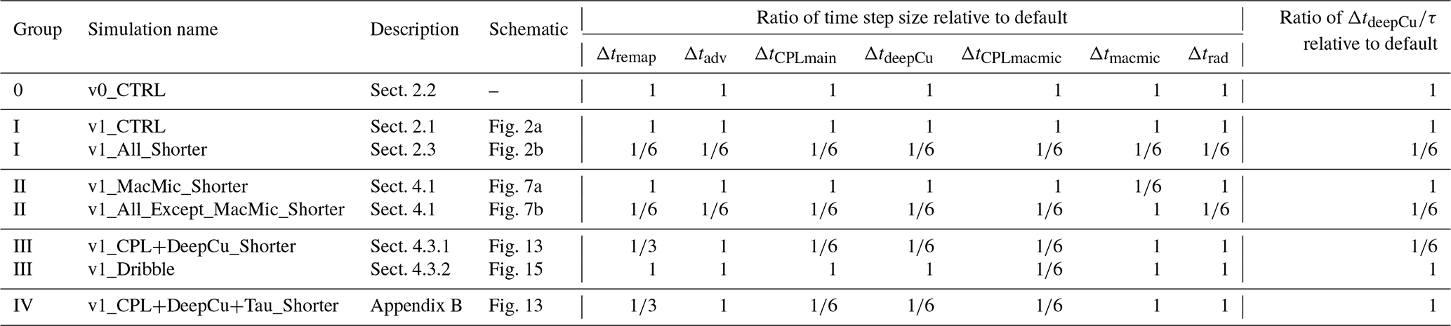
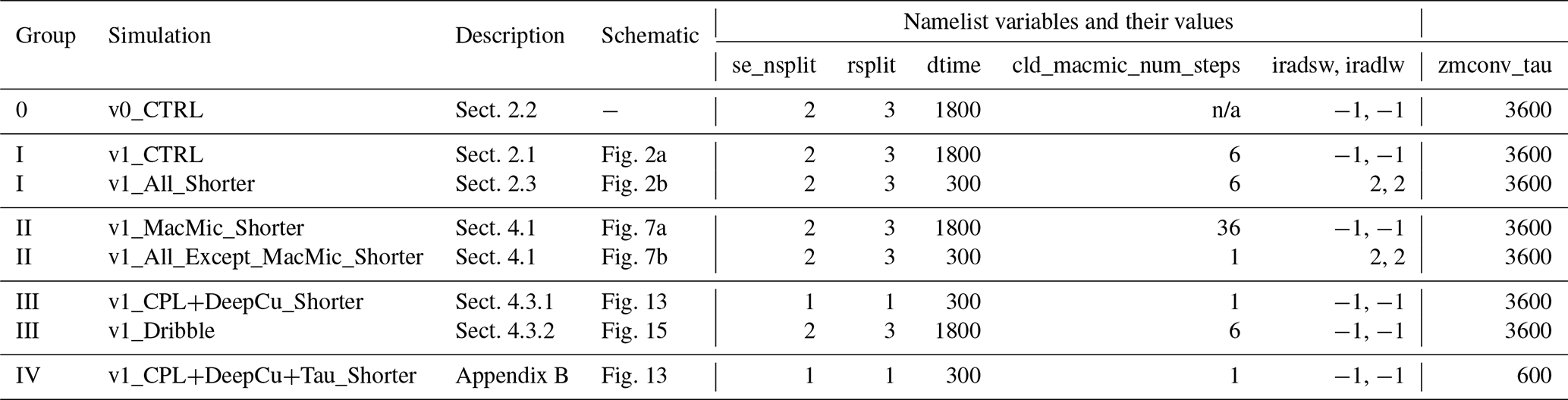
Table 1List of climate simulations conducted in this study. The numbers given in the main part of the table are the ratio of each step size (or ) relative to its value in the default 1∘ model. The meaning and default values of the various step sizes are explained in Sect. 2. Here τ refers to the prescribed (fixed) timescale in the deep convection parameterization for releasing the convective available potential energy (CAPE), the default value of which is 3600 s. The namelist variables in EAM used to configure these simulations are listed in Table A1. Schematics of the EAMv1 simulations are shown in Figs. 1, 2, 7, 13, and 15.
2.3 Present-day climate simulations
A series of 10-year simulations was conducted using an experimental setup commonly exercised in the development and evaluation of EAM and its predecessors. The model was configured to simulate recent climatological conditions by using values of the Earth's orbital conditions, aerosol emissions and greenhouse gas concentrations, land use, and sea surface temperatures and sea ice coverage characteristics of the recent past (around the year 2000). The sea surface temperature and sea ice cover were prescribed using monthly climatological values that repeated each year. Prognostic equations were integrated in time to produce evolving descriptions of the atmosphere and land states. The simulations used initial conditions written out by a previously performed multiyear simulation. Some of the model configurations used in our sensitivity experiments produced climate statistics that differed substantially from the default configuration; therefore, to avoid characterizing the initial adjustment phase, a 4-month spin-up was performed and neglected in each simulation, while the 10 subsequent years were analyzed.
Simulations were first conducted with EAMv0 or v1 using their default time steps. These are labeled v0_CTRL and v1_CTRL, respectively, in this paper. In a second v1 simulation called v1_All_Shorter (see Table 1 and the schematic in Fig. 2b), the various step sizes listed in Eqs. (1)–(4) were proportionally reduced by a factor of 6. This reduction gives a step size of 5 min for most of the parameterizations and the coupling among them, which is significantly shorter than the default but is still practically affordable for multiyear sensitivity simulations. Results from these three simulations are discussed in Sect. 3. Additional simulations were also conducted with the v1 model to allow the differences between v1_All_Shorter and v1_CTRL to be attributed to specific sets of processes and time stepping algorithms. The experimental design is summarized in Tables 1 and A1, groups II and III. The attribution process is summarized in Fig. 3, with the detailed results discussed in Sect. 4.

2.4 Statistical tests
The analyses presented in this paper focus primarily on 10-year mean annual averages. To distinguish signals of time step sensitivity from noise caused by natural variability, the two-sample t test was applied to pairs of simulations, with the test statistic constructed using annual averages. A significance level of 0.05 was chosen to determine whether differences between a pair of 10-year averages were statistically significant. This method of a two-sample t test has been used in the diagnostics package from the National Center for Atmospheric Research (NCAR) Atmosphere Model Working Group (AMWG), who developed predecessors of EAM (http://www.cesm.ucar.edu/working_groups/Atmosphere/amwg-diagnostics-package/, last access: 6 April 2021).
Considering that the sample size of 10 is relatively small, we also conducted statistical testing using monthly mean model output. Serial correlation in monthly averages was addressed by using the paired t test and the effective sample size (Zwiers and von Storch, 1995). For example, to assess the significance of the differences between simulations A and B at a certain geographical location, we used the time series of monthly mean A–B (which had 120 data points in the monthly time series) to construct the test statistic for a one-sample t test. A significance level of 0.05 was chosen to determine whether the mean of the differences was statistically zero, taking into account the autocorrelation in the time series.
We processed all the difference plots shown in the paper using both methods. The two methods turned out to give rather consistent results overall. They disagree only at a small portion of grid points associated with relatively small climate differences. The key signatures of time step sensitivity discussed below were considered statistically significant by both methods. We chose to show results from the two-sample test here to be consistent with the AMWG diagnostics package.
The first question we attempt to answer is whether the characteristics of EAMv1's present-day climate are substantially affected by the choices of time step sizes. This is done by comparing simulations v1_CTRL and v1_All_Shorter. To put the magnitude of the differences into context, we also show some representative results from v0_CTRL.
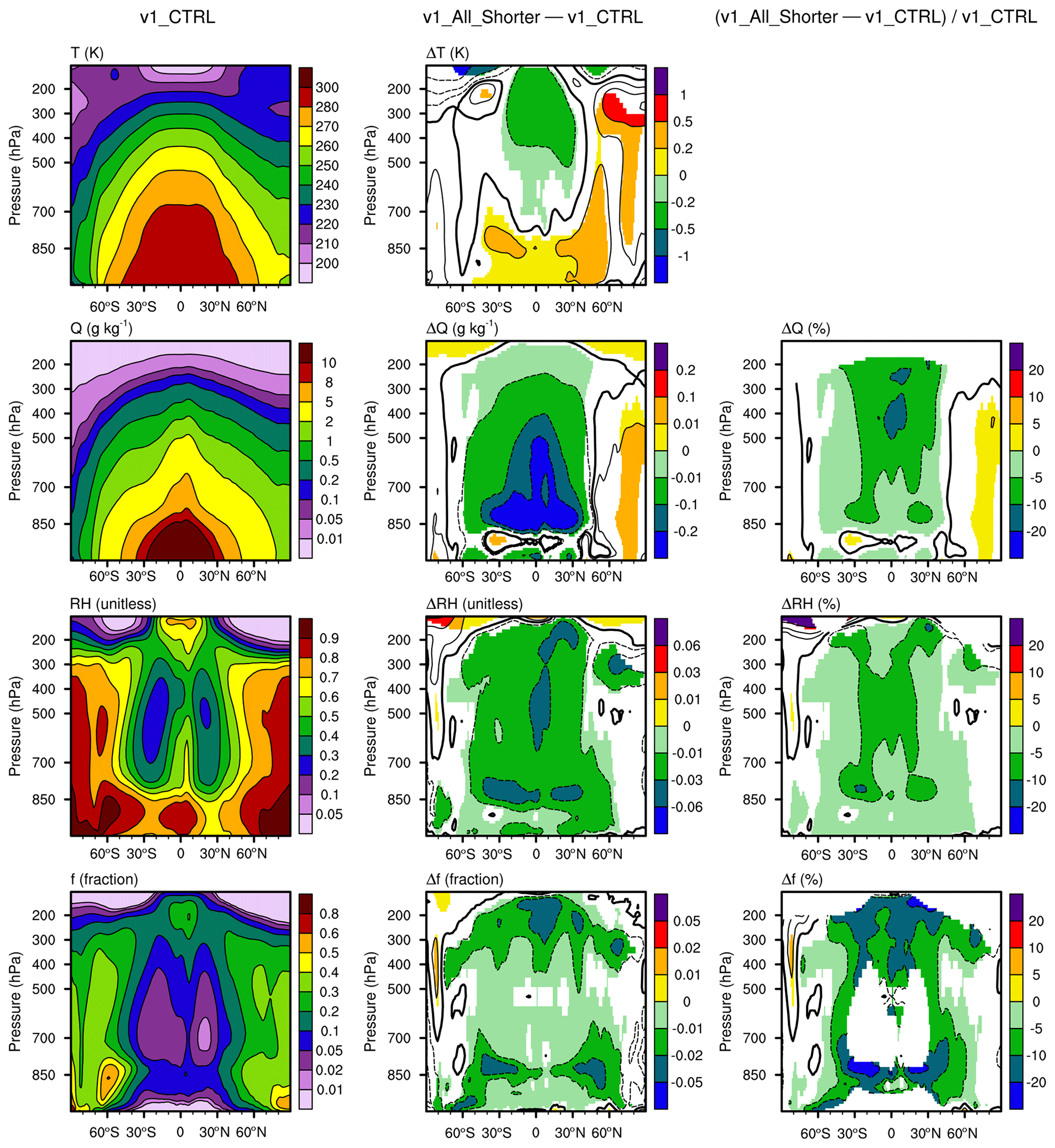
Figure 4 Left column: 10-year mean zonally averaged air temperature (T), specific humidity (Q), relative humidity (RH), and cloud fraction (f) in simulation v1_CTRL. Middle column: differences between v1_All_Shorter and v1_CTRL. Right column: relative differences with respect to v1_CTRL. Statistically insignificant differences are masked out in white. The simulation setups are described in Sect. 2.3 and also summarized in group I in Tables 1 and A1. Schematics depicting the time integration loop and different step sizes can be found in Fig. 2.
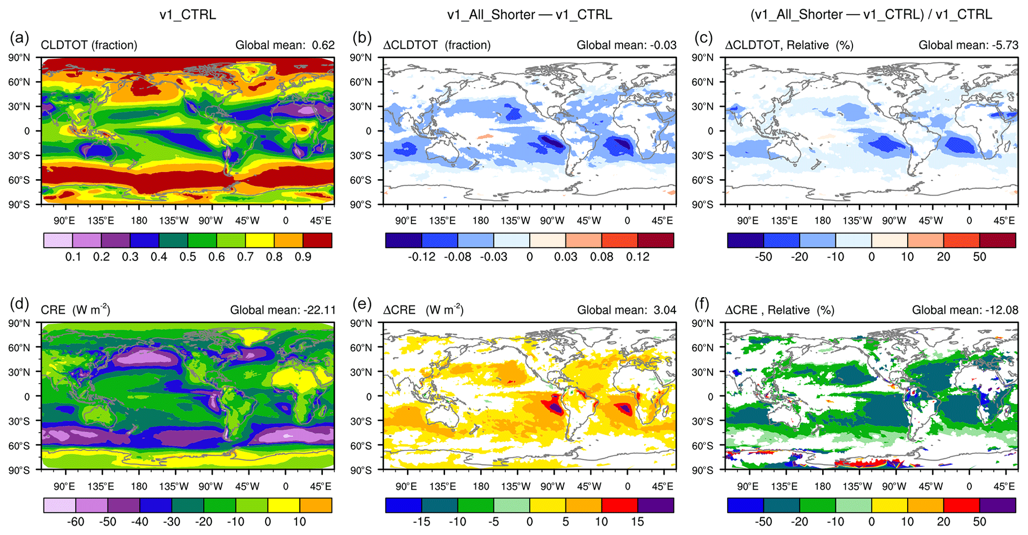
Figure 5 (a, d) The 10-year mean geographical distribution of total cloud cover (CLDTOT, a, b, c) and total cloud radiative effect (CRE, lower row) in v1_CTRL. (b, e) Differences between v1_All_Shorter and v1_CTRL. (c, f) Relative differences with respect to v1_CTRL. Statistically insignificant differences are masked out in white. The simulation setups are described in Sect. 2.3 and also summarized in group I in Tables 1 and A1. Schematics depicting the time integration loop and different step sizes can be found in Fig. 2.
3.1 Time step sensitivities in EAMv1
It turns out that the proportional factor-of-6 step size reduction in all major components of the v1 model leads to systematic changes in the simulated long-term climate. In the middle column of Fig. 4, the differences in 10-year-mean zonal averages between v1_All_Shorter and v1_CTRL are shown for air temperature (T), specific humidity (Q), relative humidity (RH), and cloud fraction (f). The relative differences normalized by corresponding values in v1_CTRL are shown in the right column. (Relative differences in T are not a useful measure and hence not included.) Statistically insignificant differences are masked out in white. The figure reveals that the step size reduction leads to warming of up to 0.5 K in the subtropical and midlatitude near-surface layers and cooling of similar magnitudes in the tropical middle and upper troposphere (Fig. 4, second panel in first row). In the middle and low latitudes, the air dries at most altitudes in the troposphere, showing typical decreases of 1 % to 10 % in both specific and relative humidity (Fig. 4, second and third rows). Cloud fraction also decreases (Fig. 4, bottom row); the largest changes appear in three regions: in the upper troposphere where ice clouds dominate, in the subtropical lower troposphere where stratocumulus and trade cumulus prevail, and in the midlatitude near-surface layers.
The 10-year mean geographical distributions of total cloud cover and total cloud radiative effect (CRE) are shown in Fig. 5. Here the signatures of time step sensitivity appear to be dominated by changes in subtropical marine stratocumulus and trade cumulus clouds. The largest local changes are on the order of −10 % to −50 % for cloud cover and −20 % to −50 % for CRE. The global mean CRE weakens by about 3 W m−2, corresponding to a relative change of −12 %.
3.2 Comparison with observations and EAMv0
A recent evaluation of EAMv1 has shown that the simulated present-day climate is cooler and drier than reanalysis in the tropical upper troposphere, while the CRE in the major marine stratocumulus regions is weaker compared to satellite products (see Figs. 3, 4, and 10 in Rasch et al., 2019). Comparing those results with the time step sensitivities shown in Figs. 4 and 5, one gets the impression that model biases in v1_All_Shorter are likely to be larger than those in v1_CTRL. Here a model bias is defined as a deviation from the real-world observation. To obtain a comprehensive yet concise assessment of the impact of time step sizes on model fidelity, we follow the spirit of Fig. 2 in Donahue and Caldwell (2018) and use the collection of reanalyses and satellite products listed in Table 6 to evaluate the fidelity of v1_CTRL and v1_All_Shorter. The results are presented in Fig. 6; the upper panel shows the relative errors in the simulated global averages, and the lower panel shows the relative errors in global patterns. The relative error in the global pattern is defined as the centered root mean square difference (RMSD) between the simulated and observed patterns normalized by the root mean square of the observed pattern. A “pattern” here refers to the annual mean global and geographical distribution of a physical quantity. The model results used in the calculations were 10-year averages. The observational data were averaged over the years indicated in Table 6. The biases in v0_CTRL are also included in the figure for comparison.
Table 2List of observational data and EAM's output variables used for evaluating model biases. The observational data were obtained from NCAR's AMWG diagnostics package (http://www.cgd.ucar.edu/amp/amwg/diagnostics/plotType.html, last access: 6 April 2021). TOA stands for “top of atmosphere”.

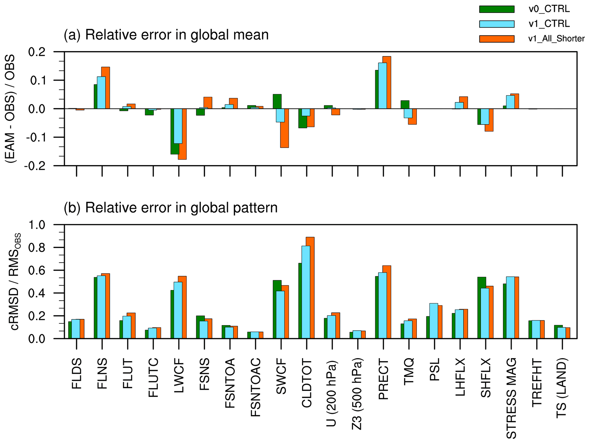
Figure 6 Comparison of 10-year mean climate simulated by v1_All_Shorter, v1_CTRL, and v0_CTRL against various reanalyses and satellite products. The upper panel (a) shows relative errors in the simulated global averages. The lower panel (b) shows the relative error in the simulated geographical distributions, as measured by the centered root mean square difference (cRMSD) between model results and the observations normalized by the root mean square of the observed global distribution (rmsOBS). The long names of the physical quantities labeled along the x axis are given in Table 2 together with the sources of observational data.
Figure 6 reveals that model biases in both the global mean (upper panel) and the spatial pattern (lower panel) are larger in v1_All_Shorter for most of the physical quantities examined here; the magnitude of the differences is comparable to the differences between v1_CTRL and v0_CTRL. For clarification, we note that v1_CTRL and v0_CTRL have different characteristic biases due to the substantial changes in the parameterizations and vertical resolution. For example, Fig. A1 shows that the shortwave CRE biases in the low latitudes are dominated by overestimation in the monsoon regions in v0 and underestimation associated with the marine stratocumulus decks and over the warm pool in v1. If we compare the local differences between v1_All_Shorter and v1_CTRL with the local differences between v0_CTRL and v1_CTRL, then the time-step-caused differences will appear to be substantially smaller than the differences caused by changes in parameterizations and vertical resolution, as should be expected. On the other hand, when comparing all three simulations (v1_All_Shorter, v1_CTRL, and v0_CTRL) with observations using the metrics shown in Fig. 6, we see that the degradation of model fidelity caused by reducing step sizes in v1 has a magnitude similar to the fidelity improvements from v0_CTRL to v1_CTRL.
Given that substantial efforts have been made to tune the default EAMv1, i.e., to adjust the values of uncertain parameters in the model's equations in order to improve the match between the simulations and observations (see, e.g., Xie et al., 2018; Rasch et al., 2019), a degradation of model fidelity associated with shortened time steps is not surprising. Assuming the time integration methods used in EAMv1 are mathematically consistent and convergent, one would expect shorter time steps to give numerically more accurate results. The results shown in Fig. 6 indicate that the default EAMv1 contains sizable time integration errors that are compensated for by parameter tuning or by other sources of model error. While the existence of compensating errors is undesirable, it is the widely recognized and accepted status quo. Reducing time integration errors would sacrifice the immediate results and temporarily degrade model fidelity, but it would also provide the opportunity to first expose and then address errors from other sources; hence, it could eventually lead to a model that gives correct results for correct reasons. As a first step towards reducing time stepping errors in EAMv1, the next section identifies the model components that have caused the differences between v1_All_Shorter and v1_CTRL. While a number of physical quantities are shown in Fig. 6, the analysis in the remainder of the paper focuses on cloud fraction and CRE. Extension of the analysis to additional variables, such as temperature, humidity, precipitation, and winds, is left to future studies.
The primary method used here for attributing the differences between v1_All_Shorter and v1_CTRL is to carry out sensitivity experiments in which we vary the step sizes used by different subsets of EAM components. These experiments are summarized in Tables 1 and A1 (see groups II and III therein) and Figs. 7, 13, and 15, and they are described in detail in the following subsections. An overview of the attribution process is provided in Fig. 3.
4.1 Stratiform cloud parameterizations versus the rest of EAMv1
The key signatures in the geographical distribution of total cloud cover and CRE changes are seen in the subtropics where marine stratocumulus and trade cumulus are the dominant cloud types (Fig. 5). Since these clouds are strongly affected by turbulence, shallow convection, and cloud microphysics, it seems natural to link the observed time step sensitivities to the corresponding parameterizations. Two hypotheses are explored here.
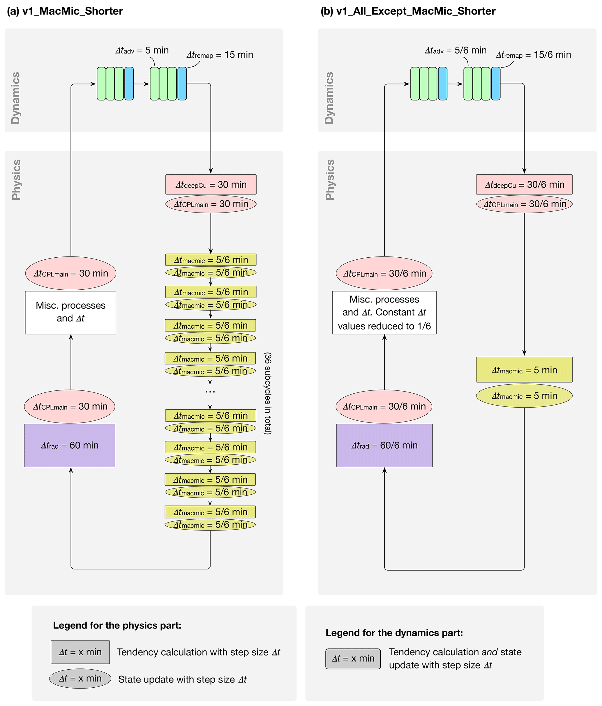
Figure 7 (a) Simulation v1_MacMic_Shorter wherein the time steps of the collectively subcycled stratiform cloud macrophysics and microphysics are shortened to of the default value, i.e., min instead of 5 min. (b) Simulation v1_All_Except_Macmic_Shorter wherein Δtmacmic is kept at its default of 5 min, while step sizes for the other parts of EAMv1 were shortened to . The color coding follows Fig. 1a. The simulation setups are summarized in Tables 1 and A1. The results are discussed in Sect. 4.1.
-
Hypothesis 1. The differences in total cloud cover and CRE seen in the subtropics between v1_All_Shorter and v1_CTRL are caused by time integration errors in the stratiform and shallow cumulus cloud macrophysics and microphysics parameterizations, i.e., CLUBB, aerosol activation, and MG2. Turbulence and cloud microphysics are known to have relatively short characteristic timescales. The 5 min step size (Δtmacmic=5 min) used in the default EAMv1 cannot sufficiently resolve those short timescales and hence gives numerically inaccurate results.
-
Hypothesis 2. The differences in total cloud cover and CRE seen in the subtropics between v1_All_Shorter and v1_CTRL are caused by time integration errors in parts of EAM other than the cloud macrophysics and microphysics parameterizations or in process coupling. In v1_All_Shorter, the reduction of time integration error in those other components, or their coupling with cloud macrophysics and microphysics, results in a different atmospheric environment being provided to CLUBB, hence triggering different responses in shallow cumulus and stratiform clouds.
The two sensitivity experiments listed in group II of Tables 1 and A1 were carried out to test the two hypotheses: simulation v1_MacMic_Shorter (see the schematic in Fig. 7a) sets the step size of the collectively subcycled shallow cumulus and stratiform cloud parameterizations, i.e., CLUBB, aerosol activation, and MG2, to of the default value, i.e, min as in v1_All_Shorter. The rest of EAMv1 used the same time integration strategy (and thus the same time step sizes) as in v1_CTRL. In other words, within each of the main coupling time steps ΔtCPLmain=30 min, instead of 6 invocations of the cloud macrophysics and microphysics parameterizations with 5 min time steps, there were 36 invocations with min time steps. The differences between results from v1_MacMic_Shorter and v1_CTRL are attributed to differences in Δtmacmic, which controls the step sizes used by CLUBB and MG2 as well as the interactions between the processes within each subcycle.
Simulation v1_All_Except_MacMic_Shorter (see the schematic in Fig. 7b) has the opposite setup, i.e., using Δtmacmic= 5 min as in v1_CTRL, while the rest of EAMv1 used the much shorter steps employed in v1_All_Shorter. The differences in model climate between v1_All_Except_MacMic_Shorter and v1_CTRL are attributed to reduced step sizes for all model components outside the cloud macrophysics and microphysics subcycles and for the coupling (i.e., information exchange) between the subcycles and the other components (compare Eqs. 1–4).
The 10-year mean difference plots shown in Figs. 8–10 indicate that the changes in long-term climate caused by Δtmacmic and the other step sizes are both non-negligible but have different signatures. The zonal mean temperature, humidity, and cloud fraction differences shown in Fig. 8 reveal the following.
-
The warming and decreases in cloud fraction around 850 hPa in the subtropics (Fig. 8a and j) are primarily attributable to shorter step sizes outside the cloud macrophysics and microphysics subcycles (Fig. 8c and l).
-
The cooling, drying, and cloud fraction decreases in the tropical middle and upper troposphere (Fig. 8a, g, and j) are attributable to shortened Δtmacmic (Fig. 8b, h, and k).
-
The decreases in cloud fraction in the midlatitude near-surface layers are also attributable to shortened Δtmacmic (Fig. 8j and k).
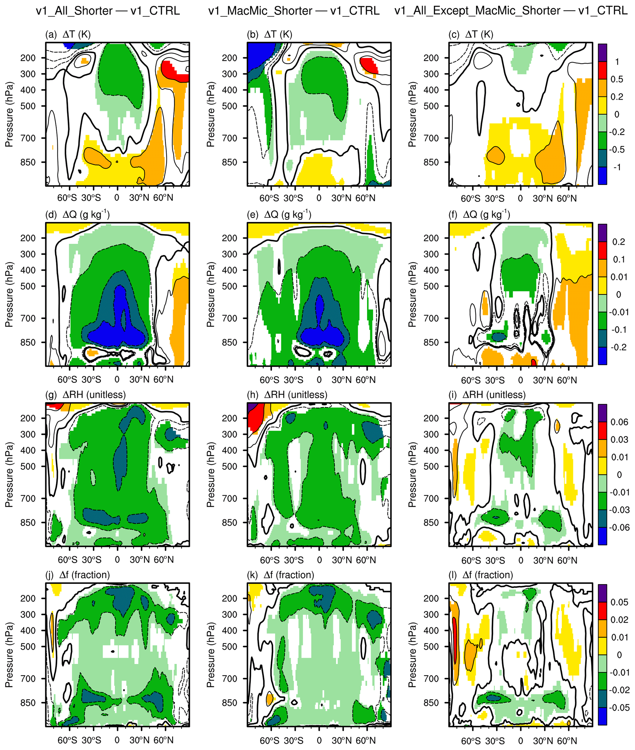
Figure 8Differences in 10-year mean zonally averaged air temperature (T), specific humidity (Q), relative humidity (RH), and cloud fraction (f) between various simulations. Left column: v1_All_Shorter – v1_CTRL, revealing the impact of shortening all major time steps listed in Eqs. (1)–(4). Middle column: v1_MacMic_Shorter – v1_CTRL, revealing the impact of shortening time steps for the subcycled cloud macrophysics and microphysics parameterizations. Right column: v1_All_Except_MacMic_Shorter – v1_CTRL, revealing the impact of shortening step sizes outside the cloud macrophysics and microphysics subcycles. Statistically insignificant differences are masked out in white. The simulation setups are summarized in Tables 1 and A1. Schematics depicting the time integration loop and different step sizes can be found in Figs. 2 and 7.
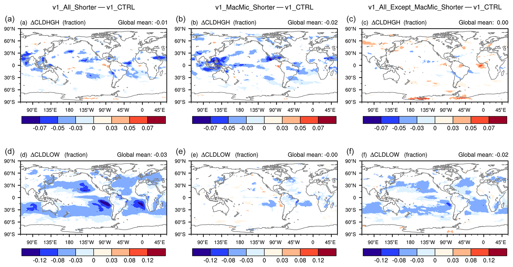
Figure 9Geographical distribution of 10-year mean differences in high-cloud fraction (CLDHGH, a, b, c) and low-cloud fraction (CLDLOW, d, e, f). (a, d) Differences between v1_All_Shorter and v1_CTRL, revealing the impact of shortening all major time steps listed in Eqs. (1)–(4). (b, e) Differences between v1_MacMic_Shorter and v1_CTRL, revealing the impact of shortening time steps for the subcycled cloud macrophysics and microphysics parameterizations. (c, f) Differences between v1_All_Except_MacMic_Shorter and v1_CTRL, revealing the impact of shortening step sizes outside the cloud macrophysics and microphysics subcycles. Statistically insignificant results are masked out in white. The simulation setups are summarized in Tables 1 and A1. Schematics depicting the time integration loop and different step sizes can be found in Figs. 2 and 7.
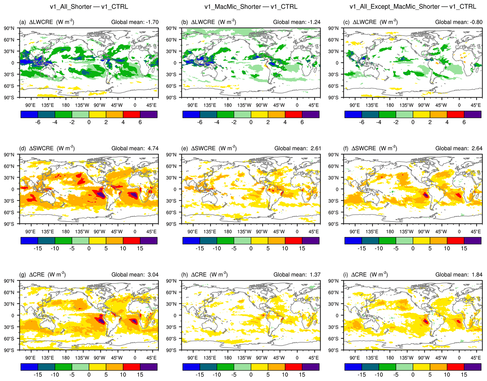
Figure 10As in Fig. 9, but showing the longwave (LW, a, b, c), shortwave (SW, d, e, f), and total (g, h, i) CRE.
Geographical distributions of high-cloud and low-cloud fraction changes are shown in Fig. 9. The corresponding LW, SW, and total CRE changes are shown in Fig. 10. Consistent with the signatures seen in the pressure–latitude cross sections in Fig. 8, one can see the major impact of Δtmacmic on high-cloud fraction (Fig. 9, top row) and LWCRE (Fig. 10, top row). The step sizes outside the cloud macrophysics and microphysics subcycles play a major role in affecting the low-cloud fraction (Fig. 9, second row) and SWCRE (Fig. 10, second row). Although reductions in the various step sizes all lead to weakening of both LWCRE and SWCRE, the total CRE changes seen in Fig. 10g are dominated by the SW changes attributable to reduced low-cloud fractions associated with shorter time steps outside the cloud macrophysics and microphysics subcycles (Figs. 10f and 9f).
These results might appear counterintuitive at first glance. Since the tropical upper troposphere is strongly affected by deep convection and the resulting detrainment of water vapor and cloud condensate, one might have assumed the sensitivities in these regions to be caused primarily by step sizes associated with the deep convection parameterization – or dynamics and other processes that introduce atmospheric instability, which in turn triggers deep convection. Yet the results shown in Figs. 8 and 9 suggest that the cloud fraction decreases in these regions are caused by shortening Δtmacmic, the step size used by turbulence, shallow convection, and stratiform clouds. A separate study has found evidence that the sensitivities in the tropical upper troposphere have to do with the representation of ice cloud microphysics in EAM. Prior work, e.g., Hardiman et al. (2015), showed that the sedimentation and depositional growth of ice particles can directly affect humidity in this region, while the optical properties and abundance of ice crystals can affect SW and LW radiation and hence temperature in the upper troposphere; how Δtmacmic affects those physical processes in EAM will be investigated in follow-up work. The link between midlatitude near-surface clouds and Δtmacmic is unclear and needs further exploration.
In the tropical and subtropical lower troposphere, Δtmacmic appears to have, as expected, significant impacts on humidity (Fig. 8e and h), cloud fraction (Fig. 9e), and CRE (Fig. 10e and h). On the other hand, for low-cloud fraction and CRE, the sensitivities to the step sizes used outside the cloud macrophysics and microphysics subcycles turn out to be substantially stronger (Figs. 9f, 10f, and i). This suggests that the low-cloud differences between v1_All_Shorter and v1_CTRL are primarily manifestations of the responses of the subcycled processes to changes in the atmospheric environment passed into the subcycles. In other words, hypothesis 2 is valid for subtropical low clouds. Next, we demonstrate in Sect. 4.2 that those low-cloud changes are associated with changes in the thermodynamic (instead of dynamic) features of the atmospheric environment. In Sect. 4.3, additional sensitivity experiments are presented to further attribute these changes to specific processes and step sizes in the rest of EAMv1.
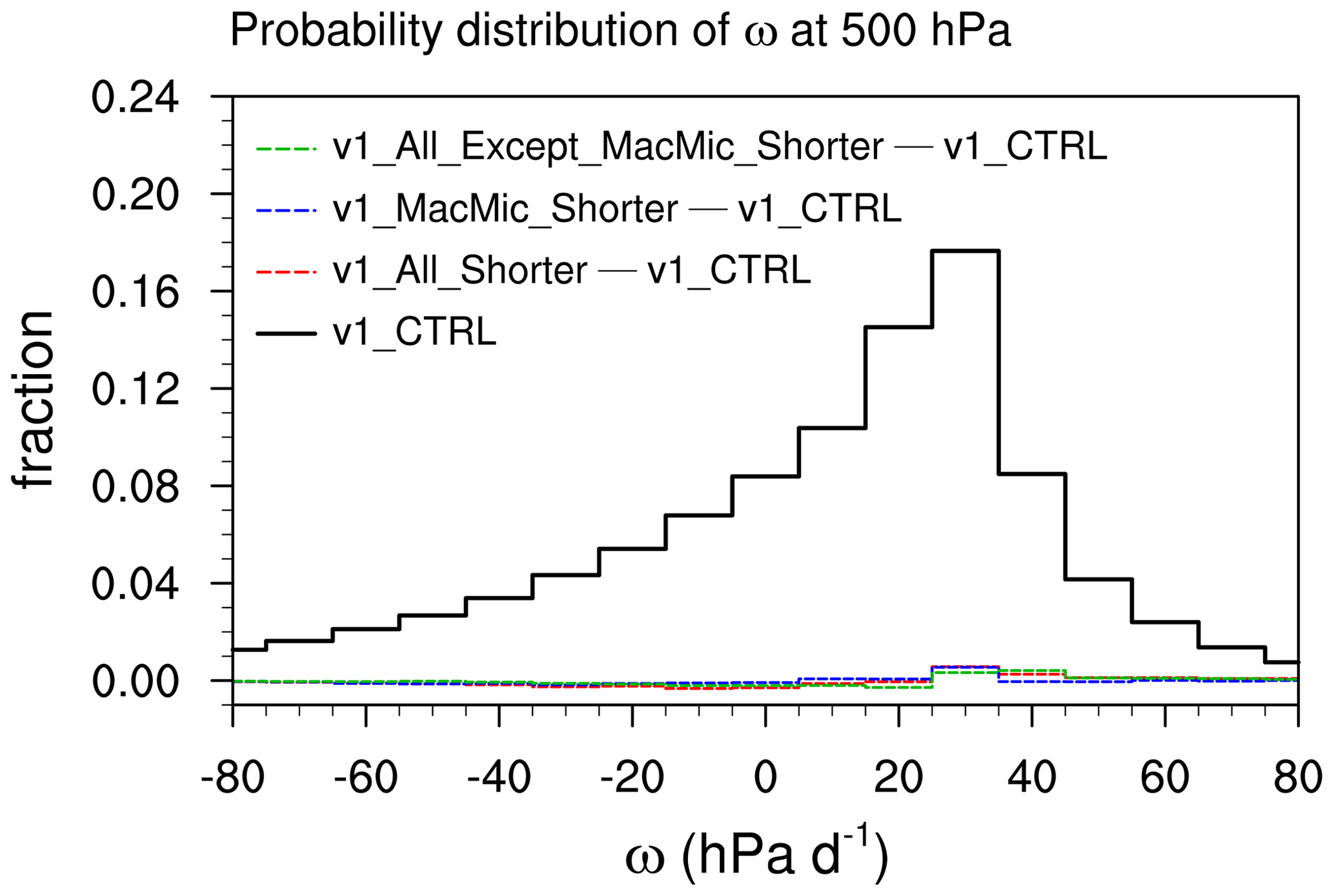
Figure 11 Frequency of occurrence of circulation regimes defined by monthly mean 500 hPa vertical velocity (ω) in the latitude band 35∘ S–35∘ N. The solid black line shows the probability distribution in v1_CTRL. Dashed colored lines show differences in the probability distribution between other simulations and v1_CTRL.
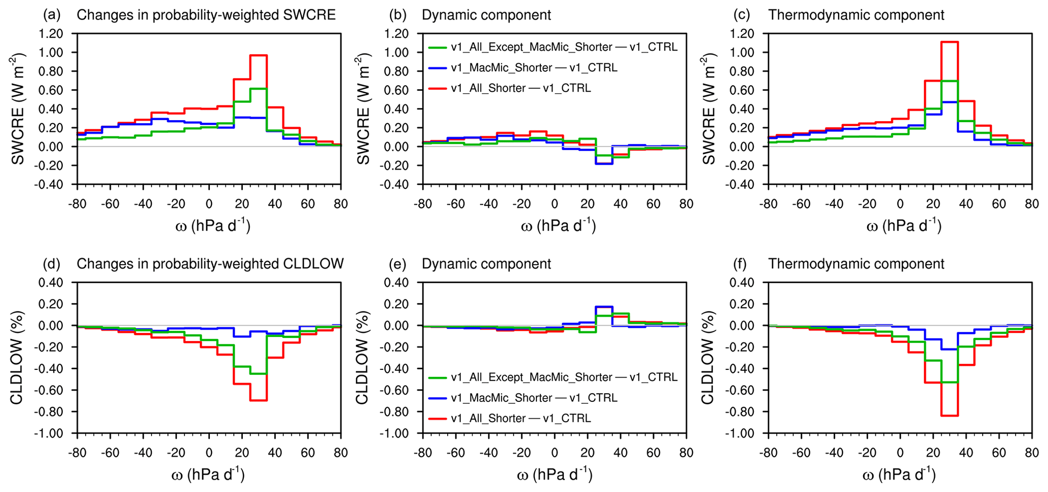
Figure 12 (a, d) Changes in the probability-weighted SWCRE (a, b, c) and low-cloud fraction (d, e, f) in circulation regimes characterized by grid-resolved 500 hPa ω (see the definitions in Eqs. 5 and 6). Panels (b, e) and (c, f) show the dynamic and thermodynamic components of the changes (see Eq. 6). Details of the analysis can be found in Sect. 4.2.
4.2 Dynamic versus thermodynamic responses of the subtropical climate
Large-scale subsidence is one of the key features of the subtropical climate. To find out whether the reduced low-cloud fraction and weaker CRE in v1_All_Shorter are associated with weakened subsidence, the method from Bony et al. (2004) is used to compare the dynamic and thermodynamic components of the low-cloud changes.
We first examined the geographical distribution of grid-resolved vertical velocity ω at 500 hPa. The differences among the various simulations discussed so far appeared to be rather small and statistically insignificant; hence, they are not shown here. The conclusion of insignificant changes in vertical velocity can also be inferred from the frequency of occurrence of 500 hPa ω, denoted here as Pω, shown in Fig. 11. Here, Pω is diagnosed using monthly mean grid-point-by-grid-point ω values in the latitude band of 35∘ S to 35∘ N. The solid black line in Fig. 11 is Pω in v1_CTRL; the dashed colored lines show differences in Pω between other simulations and v1_CTRL. The differences appear to be close to zero compared to Pω in v1_CTRL.
We then followed Bony et al. (2004) and defined circulation regimes using monthly mean ω. For a circulation regime associated with ω values between ω1 and ω2, we refer to the integral of a generic physical quantity ψ weighted by the probability density function p(ω) as the probability-weighted ψ, i.e.,
Following Bony et al. (2004), changes in the probability-weighted ψ can be decomposed as follows.
In Fig. 12, we present changes in the probability-weighted low-cloud fraction and SWCRE in the left column and their decomposition in the middle and right columns. The results suggest that the low-cloud fraction and SWCRE changes in regions associated with subsidence can be attributed primarily to the thermodynamic responses of the model atmosphere instead of vertical velocity changes.
4.3 Further attribution of subtropical low-cloud changes
In earlier sections, it has been shown that the reduction in subtropical marine low-cloud fraction and CRE in v1_All_Shorter are caused primarily by the use of shorter time steps for model components and their coupling (i.e., information exchange) outside the cloud macrophysics and microphysics subcycles. We now make an attempt to refine the granularity of the attribution. Additional sensitivity experiments are discussed in this subsection and summarized as group III in Tables 1 and A1. An overview of the attribution process is provided in Fig. 3 with pointers to the figures that show the results.
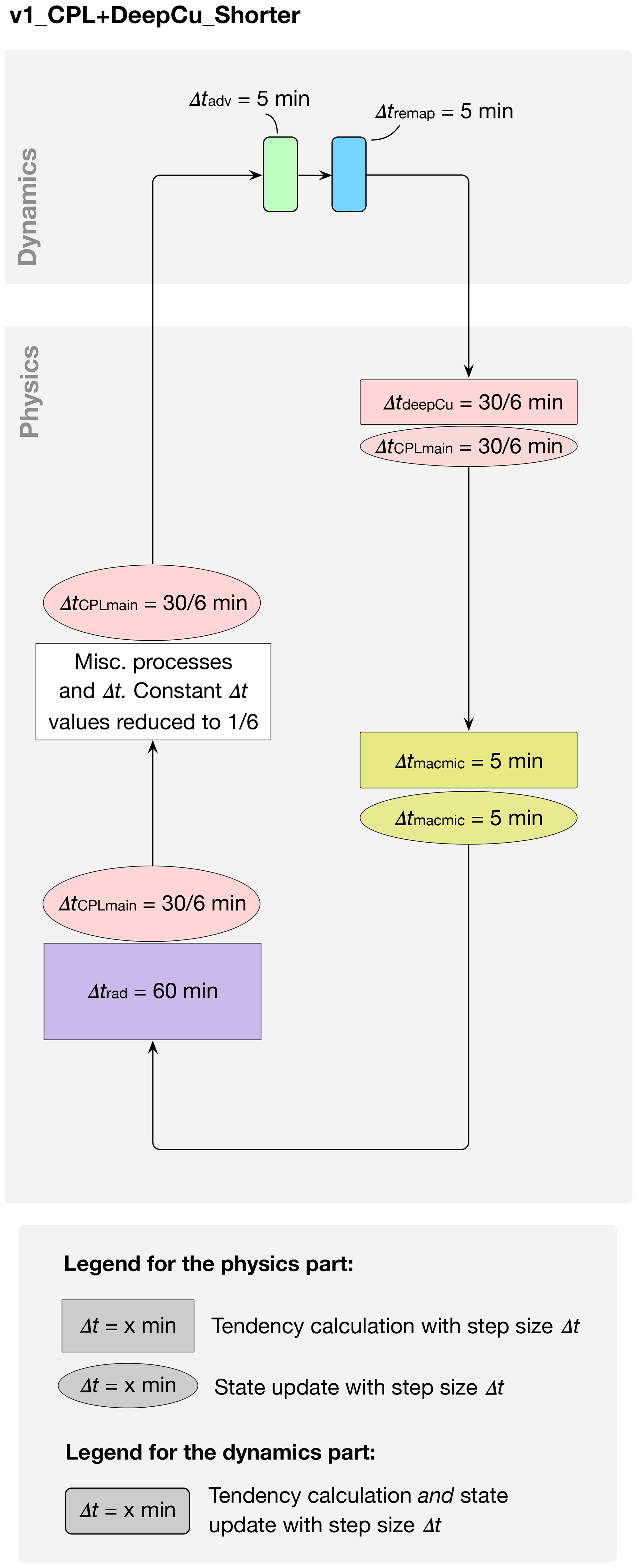

Figure 14The 10-year mean CRE differences between simulations v1_All_Except_MacMic_Shorter (see the schematic in Fig. 7b) and v1_CPL+DeepCu_Shorter (see the schematic in Fig. 13), revealing the impact of shortened dynamics and radiation time steps. White indicates statistically insignificant differences. The simulation setups are summarized in Tables 1 and A1.
4.3.1 Resolved dynamics and radiation
A simulation labeled v1_CPL+DeepCu_Shorter in Tables 1 and A1 (see the schematic in Fig. 13) was configured to be the same as v1_All_Except_MacMic_Shorter (schematic in Fig. 7b) except that Δtadv (the horizontal advection time step in the dynamical core) and Δtrad (the interval for calculating radiative cooling and heating rates) are reverted to their default values in v1_CTRL.1 The comparison of this pair of simulations reveals the impact of Δtadv and Δtrad, as shown in Fig. 14. The CRE differences appear to have small and mostly insignificant magnitudes. The small yet systematic differences in LWCRE in the Southern Hemisphere midlatitudes (Fig. 14a) indicate a shift in the location of the storm tracks, but no systematic signals are seen in the lower latitudes. Therefore, we conclude that the impact of dynamics and radiation time steps on subtropical clouds is small, at least in the context of the currently used process ordering and splitting–coupling methods.
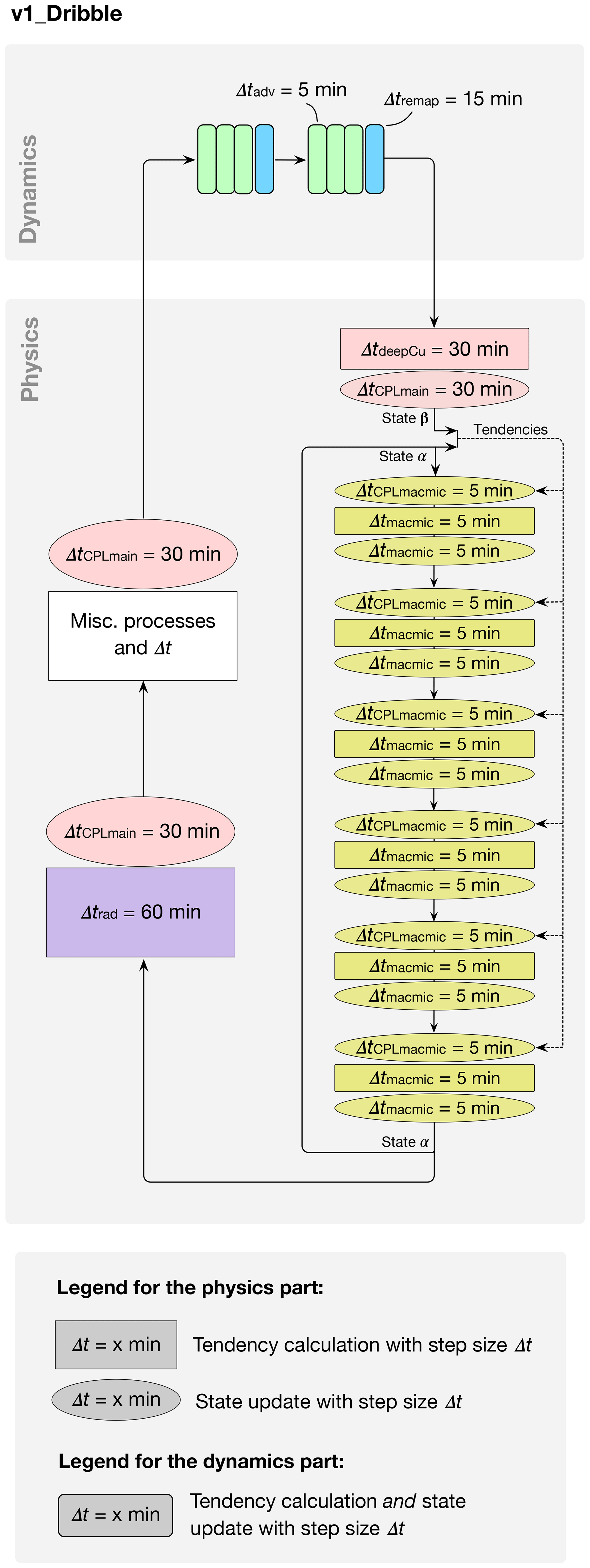

Figure 16 (a, c, e) Differences between v1_Dribble (see the schematic in Fig. 15) and v1_CTRL (see the schematic in Fig. 2), revealing the impact of coupling between the subcycled cloud macrophysics–microphysics and the rest of EAM. (b, d, f) Differences between v1_CPL+DeepCu_Shorter (see the schematic in Fig. 13) and v1_Dribble (see the schematic in Fig. 15), revealing the impact of step sizes used by various other parameterizations (deep convection, gravity wave drag, miscellaneous aerosol processes) and the coupling among them. White indicates statistically insignificant differences. The simulation setups are summarized in Tables 1 and A1.
4.3.2 Coupling between cloud macrophysics–microphysics and other processes
Since Sect. 4.3.1 has shown that the step sizes of resolved dynamics and radiation time steps have only very limited impacts, we are left with two step sizes to explore, ΔtCPLmain and ΔtdeepCu, to answer the question of which step sizes outside the cloud macrophysics and microphysics subcycles are responsible for the subtropical CRE changes shown in the rightmost column of Fig. 10. As explained in Sect. 2 and illustrated by color coding in Fig. 2a, these two step sizes have the same value in EAMv1, and the single ΔtCPLmain also controls the coupling frequency among the majority of the parameterizations as well as between physics and dynamics. This makes further attribution somewhat difficult unless changes are made to the model source code. Nevertheless, our exploration revealed that the coupling between the subcycled cloud parameterizations and the rest of the model was impactful.
Figure 15 shows the schematic for a simulation called v1_Dribble, which uses EAMv1's default step sizes for all the individual model components but a revised scheme for the coupling between the stratiform cloud subcycles and the rest of the model. In the revised scheme, the atmospheric temperature, specific humidity, and cloud liquid and ice concentrations that are passed to the first cloud macrophysics–microphysics subcycle are no longer the values updated by deep convection and dynamics (i.e., no longer state β in Fig. 15). Instead, the older snapshot saved after the last (i.e., sixth) 5 min cloud macrophysics–microphysics subcycle in the previous main time step (state α in Fig. 15) is provided together with the tendencies caused by all processes between points α and β in the schematic. At the beginning of each subcycle, those tendencies are used to update the atmospheric state using a step size of 5 min, as illustrated by the greenish-yellow ovals labeled with ΔtCPLmacmic=5 min in Fig. 15. This “dribbling” method is conceptually similar to the physics–dynamical coupling scheme used by EAMv1's dynamical core for temperature and horizontal winds (Zhang et al., 2018; Rasch et al., 2019), and it is also similar to the two other instances of tendency-involved process coupling mentioned at the end of Sect. 2.1. This dribbling can be viewed as an example of the sequential-tendency splitting method defined in Donahue and Caldwell (2018). To help distinguish this dribbling from the original splitting method depicted in Fig. 2a, we introduced the notation ΔtCPLmacmic in Eq. (2) and Fig. 15 as well as in Table 1 and Fig. 3; ΔtCPLmacmic=30 min in v1_CTRL and 5 min in v1_Dribble.
Dribbling provides a more frequent coupling from the perspective of the subcycled cloud macrophysics–microphysics, while the feedback to the processes outside the subcycles still occurs at longer intervals of ΔtCPLmain. A detailed explanation of the motivation for this dribbling and an in-depth analysis of its impact on the atmospheric water budget will be the topic of a separate paper. Here we only show the CRE differences between the two simulations v1_Dribble and v1_CTRL in the left column of Fig. 16. Weakened SWCRE and total CRE are found over the eastern parts of the subtropical oceans, especially in the Peruvian and Namibian stratocumulus regions. This suggests that the strongest local reduction of SWCRE and/or total CRE seen earlier in simulation v1_All_Except_MacMic_Shorter (Fig. 10f and i) is primarily attributable to more frequent coupling between the subcycled cloud macrophysics–microphysics and the rest of EAM.
4.3.3 Deep convection
We now attempt to attribute the time step sensitivities seen in simulation v1_All_Except_MacMic_Shorter (Fig. 10, right column) that are not explained by dribbling (Fig. 16, left column) or the time steps of dynamics and radiation (Fig. 14). This can be done by comparing the simulations v1_CPL+DeepCu_Shorter introduced in Sect. 4.3.1 and v1_Dribble discussed in Sect. 4.3.2, as the two experiments share the same Δtadv, Δtrad, and ΔtCPLmacmic, while they differ in the step sizes used for deep convection and its coupling to other processes, as well as miscellaneous processes like land surface, gravity wave drag, aerosols, and the coupling among them.
The right column in Fig. 16 shows the 10-year mean differences in CRE, revealing weaker LWCRE and SWCRE along the equatorial ITCZ (Intertropical Convergence Zone, where deep convection is important) and in the subtropics and equatorward flanks of the storm tracks. The LW and SW changes largely cancel each other along the Equator and near the storm tracks, leaving differences in the net CRE visible only in the trade cumulus regions. The signatures of a net cancellation in LWCRE and SWCRE along the ITCZ provide hints that there is a change in behavior in the deep convection regime.
Similar to the discussions in earlier sections on the stratiform cloud parameterizations, time step sensitivities associated with the deep convection parameterization can potentially be caused by the temporal truncation errors inside the parameterization, the coupling between the parameterization and other model components, or both. In the default EAMv1 and its recent predecessors, no subcycles are used for deep convection, meaning that the convection time step ΔtdeepCu and coupling time step ΔtCPLmain are tied together. Therefore, without further code modifications and simulations, we cannot yet further attribute the sensitivities seen in the right column of Fig. 16. Williamson (2013) discussed how the interplay between convection and stratiform clouds can be affected by their corresponding timescales and the model time step. Based on that study, one can speculate that process coupling might be an important cause of the sensitivities seen in the right column of Fig. 16. Whether this is indeed the case needs to be verified in future studies. Here we only make a brief comment that while the results in Williamson (2013) are commonly interpreted as the deep convection parameterization being constrained by the assumed timescale, our preliminary exploration described in Appendix B suggests that the time step–timescale ratio alone cannot explain the changes in CRE shown in the right column of Fig. 16. There are other significant factors related to process coupling that need to be identified and understood in the future.
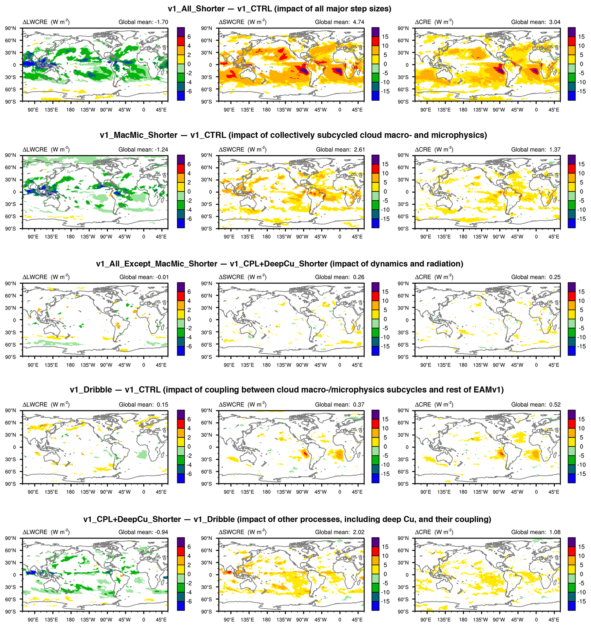
Figure 17 Attribution of the 10-year mean CRE differences between v1_All_Shorter and v1_CTRL (first row) to various components of EAMv1 (lower rows). Left column: LWCRE; middle column: SWCRE; right column: total CRE. White indicates statistically insignificant differences. The attribution process is summarized in Fig. 3. The simulation setups are summarized in Tables 1 and A1. Schematics depicting EAM's time integration loop and different step sizes can be found in Figs. 2, 7, 13, and 15.
This study evaluated the strength of time step sensitivities in 10-year present-day climate simulations conducted with the EAMv1 atmospheric model at 1∘ horizontal resolution. A proportional factor-of-6 reduction of time step size in major components of the model (simulation v1_All_Shorter versus v1_CTRL) was found to result in changes in the long-term mean climate that were significant both statistically and physically. A systematic warming was found in the low-latitude areas in the near-surface levels and a systematic cooling was seen aloft, with 10-year zonal mean temperature differences of up to 0.5 K. The zonal mean relative humidity was found to decrease by 1 %–10 % throughout the troposphere. Sizable zonal mean cloud fraction decreases were seen at most latitudes in the upper troposphere (10 %–20 %), the subtropical lower troposphere (more than 20 %), and the midlatitude near-surface layers (10 %–20 %). In terms of geographical distribution, the most pronounced annual mean changes are the decreases in total cloud cover (10 %–50 %) and CRE (20 %–50 %) over the subtropical marine stratocumulus and trade cumulus regions. The global mean CRE weakens by about 3 W m−2, corresponding to a relative decrease of 12 %.
The comparison of model results with a comprehensive set of observational data indicated that the changes caused by step size reduction led to a degradation in model fidelity in terms of both the global mean statistics and the geographical distributions. Although this is not surprising given the careful tuning EAMv1 has undergone, the compensation for time integration error by parameter tuning or by other sources of model error is undesirable. This compensation implies the need for additional tuning to achieve a new compensation when model time steps are shortened for high-resolution simulations. It would be more desirable to identify time stepping algorithms with numerical errors that are small enough that the simulation fidelity is insensitive to reasonable variations in step size: that is, so that the simulation quality is determined by physical understanding (or lack thereof).
In order to provide clues for future efforts to reduce time stepping errors in EAM, additional simulations were conducted to tease out some of the sources of time step sensitivities seen in EAMv1. Most of those simulations made use of flexible choices of time step sizes currently available in various subsets of EAM components. One of the simulations (v1_Dribble) used an alternate numerical scheme to couple the collectively subcycled shallow cumulus and stratiform cloud macrophysics–microphysics parameterizations with the rest of EAM at a higher frequency. A simulation discussed in Appendix B used a different value for the CAPE removal timescale in the deep convection parameterization to investigate the impact of the ratio of time step to this timescale.
Analysis of the results focused primarily on the annual mean cloud fraction and CRE. We found that the most notable sensitivity in the simulations was a change in total cloud cover and CRE in the subtropical marine stratocumulus and trade cumulus regimes. Our analysis revealed that this sensitivity was not caused primarily by the step size used for treating some of the most important processes in those regimes (turbulence, shallow cumulus, and stratiform cloud macrophysical and microphysical processes; see simulation v1_MacMic_Shorter) but rather by the strategy used to couple those processes to other components of the model (see simulation v1_Dribble). On the other hand, the step size of the cloud macrophysics and microphysics subcycles had quite an important impact on cloud fraction at most latitudes in the upper troposphere between 100 hPa and 400 hPa, as well as in the midlatitude near-surface layers. Additional simulations and analysis revealed that the deep convection parameterization and its coupling with other processes significantly affected trade cumulus. Impacts of the step sizes used by the dynamical core and radiation were small. In Fig. 17, we have reorganized some of the CRE difference plots presented in earlier sections: a different panel layout is used to facilitate a direct comparison of the impacts of step sizes used by different model components. Recent follow-up and independent studies have provided insights into the impact of process coupling on marine stratocumulus clouds and the impact of the macrophysics–microphysics time step on ice cloud formation. Those results will be reported in separate papers. The mechanisms behind the other sensitivities shown in the figure still need to be investigated.
Using the analysis method of Bony et al. (2004), we found that the subtropical low-cloud changes were primarily local thermodynamic responses of the model atmosphere, while the impact of circulation (vertical velocity) changes was very small. This conclusion has practical implications for follow-up investigations: since circulation changes are negligible and local cloud processes are fast, it should be feasible to use nudged 1-year simulations (Kooperman et al., 2012; Zhang et al., 2014; Sun et al., 2019) or even ensemble simulations of a few days (Xie et al., 2012; Ma et al., 2013; Wan et al., 2014) to help carry out further investigations at the process level and meanwhile keep the numerical experiments computationally economical.
Coincidentally, when our paper was submitted to Geoscientific Model Development, a paper by Santos et al. (2020a) was submitted to a different journal, which described an independent study that also attempted to quantify and attribute time step sensitivities in EAMv1. Their experimental strategy and ours turned out to be similar, although the details differed. Their analysis had a stronger focus on global mean precipitation rates and zonal mean cloud amounts, whereas our attribution focused more on the geographical distribution of CRE.
While both this study and the work of Santos et al. (2020a) focused on one specific AGCM, it would be useful to carry out similar exercises with other models. Because of considerations of computational cost, numerical models used for operational weather forecasts and climate research generally tend to use the longest step sizes that would provide satisfactory results. The chosen step sizes, however, influence key simulated features to an extent that is not always clear. If a time step sensitivity quantification exercise like ours presented in Sect. 3 reveals strong sensitivities, that would provide a motivation to understand the causes of the sensitivities and, in the next step, revise the numerical methods to provide higher accuracy without substantially increasing the computational cost.
Table A1 documents the namelist settings used in the EAMv0 and EAMv1 simulations presented in this paper. Figure A1 presents the geographical distribution of SWCRE biases in v0_CTRL and v1_CTRL to show that the two models have different characteristics in the spatial distribution of model biases (see Sect. 3.2).
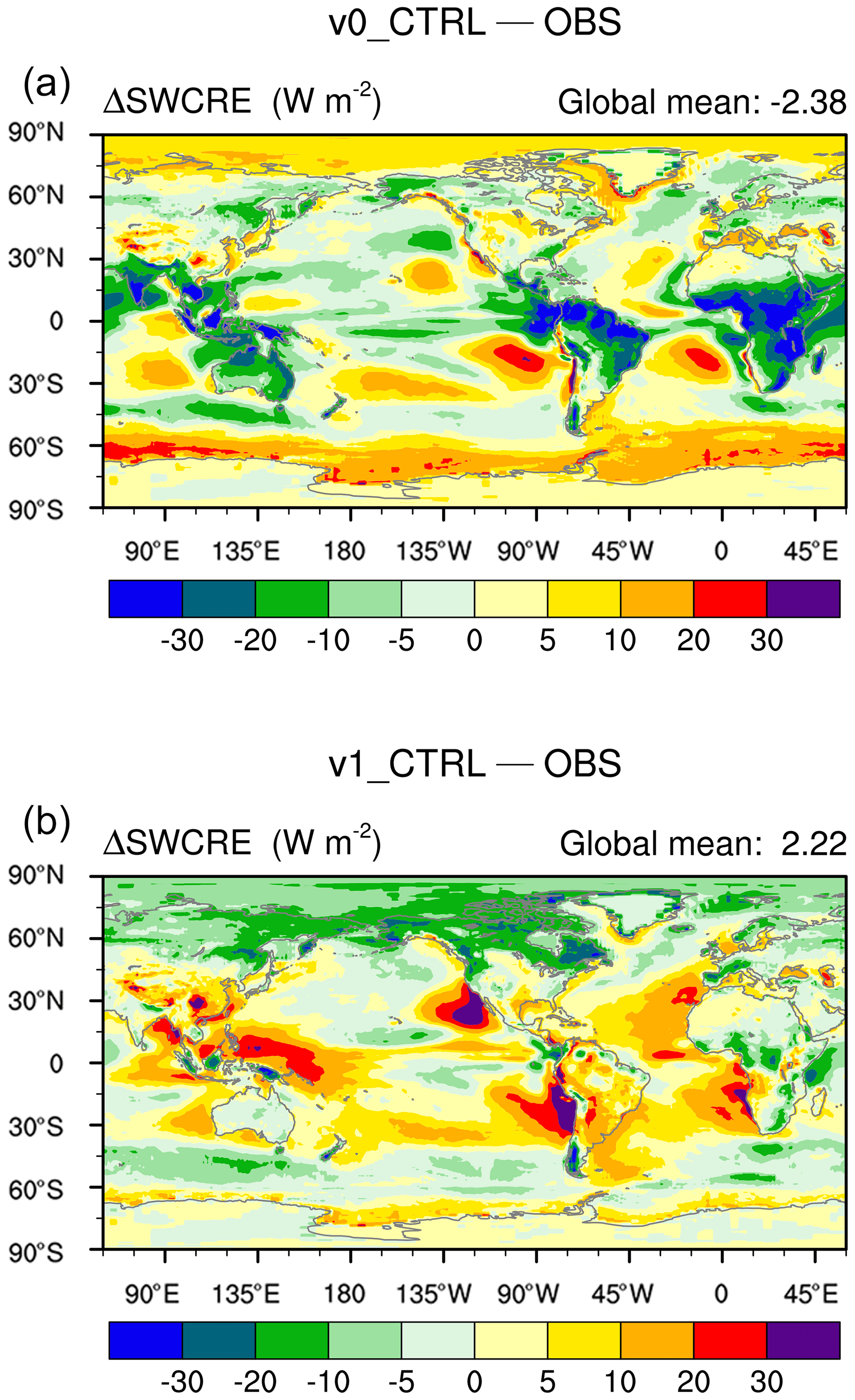
Figure A1The 10-year mean differences in SWCRE between simulation v0_CTRL (a) and v1_CTRL (b) as well as the 2000–2010 averages from CERES-EBAF.
Table A1Namelist setups used for the simulations listed in Table 1; n/a means not applicable.
Section 4.3.3 noted time step sensitivities in the deep convection regime but was inconclusive on the cause of such sensitivities. Based on the work of Williamson (2013), one can speculate that the interactions between deep convection and stratiform cloud parameterizations might be an important factor. In this Appendix, we present some preliminary results to show that how those interactions affect time step sensitivities in the deep convection regime is a complex topic that needs further investigation.
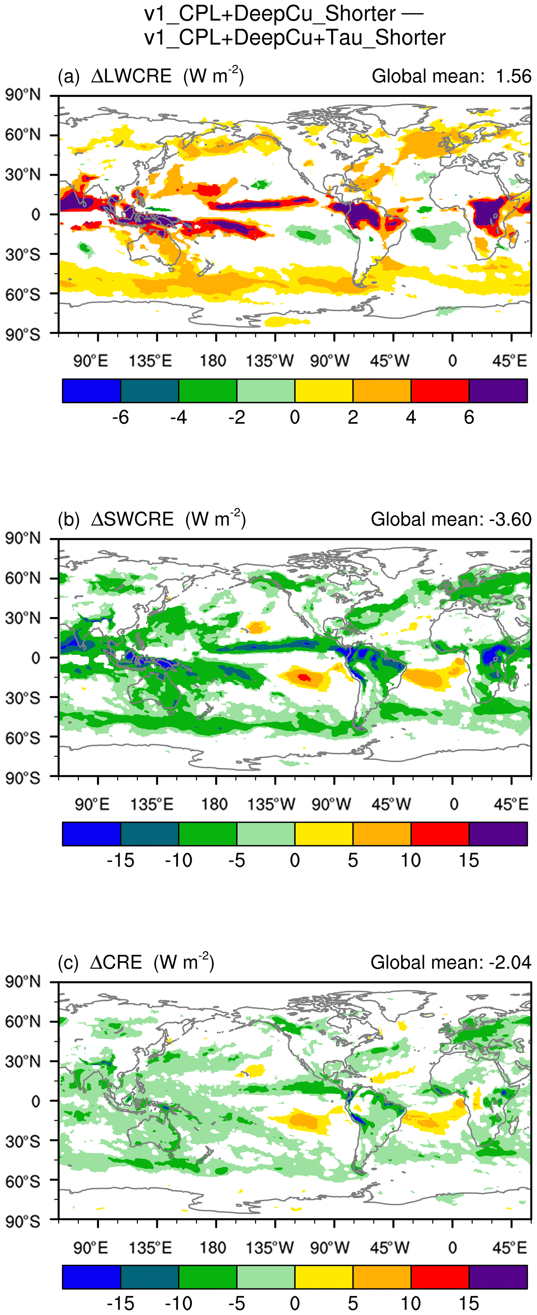
Figure B1 The 10-year annual mean CRE differences between v1_CPL+DeepCu_Shorter and v1_CPL+DeepCu+Tau_Shorter, revealing the impact of a reduced ratio of without model step size changes. White indicates statistically insignificant differences. The simulation setups are summarized in Tables 1 and A1. The two simulations correspond to the same schematic shown in Fig. 13.
Williamson (2013) pointed out that convective parameterizations designed to remove instability and supersaturation on a fixed timescale of τ are constrained by its step size in how much work such parameterizations can do in each time step. In contrast, large-scale condensation parameterizations designed to completely remove supersaturation within every time step are unconstrained, with implications for the column instability and depth of convection that in turn affects the resolved dynamical response. This difference in characteristic behavior can affect the simulated interactions between dynamics, deep convection, and the stratiform cloud processes. Williamson (2013) showed that this time step–timescale issue ( issue) could explain the occurrence of intense truncation-scale storms in high-resolution simulations conducted with the Community Atmosphere Model version 4 (CAM4). Other studies, e.g., Mishra et al. (2008), Mishra and Srinivasan (2010), Mishra and Sahany (2011), Yang et al. (2013), Qian et al. (2015), Yu and Pritchard (2015), Lin et al. (2016), and Qian et al. (2018), have also shown model sensitivities to Δt and/or τ.
Here, it is worth noting again that in the default EAMv1 and its recent predecessors, including CAM4 used in Williamson (2013), no subcycles are used for deep convection, meaning that the step size used by each invocation of the convection parameterization is the same as the step size used for the coupling of deep convection with other model components. In other words, Δt in Williamson (2013) is both ΔtdeepCu and ΔtCPLmain in this paper and we have ΔtdeepCu≡ΔtCPLmain in these models.
It is also worth noting that the ratio of can be changed through the denominator, numerator, or both. The direct effects of varying τ are limited to the ratio and the strength of convective activity the ratio controls, while a different Δt will also change the temporal truncation error associated with the deep convection scheme and process coupling.
The impact of a smaller ratio caused by changing only the timescale τ can be derived by comparing the simulation v1_CPL+DeepCu_Shorter introduced in Sect. 4.3.1 and a new simulation, v1_CPL+DeepCu+Tau_Shorter. Both experiments used the same step sizes depicted in the schematic in Fig. 13, but the values of τ differed by a factor of 6; hence, the ratio in v1_CPL+DeepCu_Shorter is of the ratio in v1_CPL+DeepCu+Tau_Shorter. A smaller ratio decreases the relative importance of the convective parameterization per time step and therefore amplifies the role of the stratiform cloud parameterizations and associated Hadley circulation; this makes the positive LWCRE more positive and the negative SWCRE more negative in convective regions. In other words, the strengthened amplitudes of both LW and SW CRE in the ITCZ seen in Fig. B1 are consistent with the response described in Williamson (2013).
In contrast, the right column of Fig. 16 in Section 4.3.3 shows CRE changes corresponding to a factor-of-6 decrease in the ratio caused by shortening Δt; the signs and patterns of CRE changes in the ITCZ are different from what is seen in Fig. B1. The discrepancies between the two figures suggest that the more frequent invocation of deep convection and more frequent coupling with other processes have led to consequences that compensate (in fact overcompensate) for the impact of a smaller . In other words, the overall responses of the annual mean CREs to a shortened Δt are inconsistent with the time step–timescale argument in Williamson (2013).
The EAMv0 and v1 source codes and run scripts used in this study can be found on Zenodo at https://doi.org/10.5281/zenodo.4118705 (E3SM developers et al., 2020).
The EAMv0 and v1 model output used in this study can be found on Zenodo at https://doi.org/10.5281/zenodo.4668866 (Zhang and Wan, 2021).
HW initiated this study and designed the sensitivity experiments with input from the coauthors. HW conducted the EAMv0 simulation. SZ carried out the EAMv1 simulations and processed all the model output. HW and SZ led the analysis of the results, and the other authors provided feedback. HW wrote the first draft of the paper and led the subsequent revisions. All coauthors contributed to the revisions.
The authors declare that they have no conflict of interest.
The authors thank Kai Zhang for helpful discussions during this study and for his comments on various versions of the paper. Andrew Barrett and an anonymous referee are thanked for their insightful reviews, which helped to substantially improve the clarity of the paper. Computing resources were provided by the National Energy Research Scientific Computing Center (NERSC), a U.S. Department of Energy Office of Science User Facility operated under contract no. DE-AC02-05CH11231. The Pacific Northwest National Laboratory is operated for the DOE by the Battelle Memorial Institute under contract DE-AC06-76RLO 1830.
This research has been supported by the U.S. Department of Energy, Office of Science, Office of Biological and Environmental Research (BER), via the Scientific Discovery through Advanced Computing (SciDAC) program (grant no. 70276).
This paper was edited by Paul Ullrich and reviewed by Andrew Barrett and one anonymous referee.
Barrett, A. I., Wellmann, C., Seifert, A., Hoose, C., Vogel, B., and Kunz, M.: One Step at a Time: How Model Time Step Significantly Affects Convection-Permitting Simulations, J. Adv. Model. Earth Sy., 11, 641–658, https://doi.org/10.1029/2018MS001418, 2019. a
Beljaars, A., Bechtold, P., Köhler, M., Morcrette, J. J., A.Tompkins, Viterbo, P., and Wedi, N.: The numerics of physicalparameterization, in: Seminar on Recent Developments in Numerical Methods for Atmospheric and Ocean Modelling, European Centre For Medium-Range Weather Forecasts, Shinfield Park, Reading, United Kingdom, ECMWF, 2004. a, b
Beljaars, A., Dutra, E., Balsamo, G., and Lemarié, F.: On the numerical stability of surface–atmosphere coupling in weather and climate models, Geosci. Model Dev., 10, 977–989, https://doi.org/10.5194/gmd-10-977-2017, 2017. a
Beljaars, A., Balsamo, G., Bechtold, P., Bozzo, A., Forbes, R., Hogan, R. J., Köhler, M., Morcrette, J.-J., Tompkins, A. M., Viterbo, P., and Wedi, N.: The Numerics of Physical Parametrization in the ECMWF Model, Front. Earth Sci., 6, 137, https://doi.org/10.3389/feart.2018.00137, 2018. a, b
Beljaars, A. C. M.: Numerical schemes for parametrizations, in: Seminar on Numerical Methods in Atmospheric Models, European Centre For Medium-Range Weather Forecasts, Shinfield Park, Reading, 1–42, available at: https://www.ecmwf.int/node/8028 (last access: 6 April 2021), 1991. a
Bogenschutz, P. A., Gettelman, A., Morrison, H., Larson, V. E., Craig, C., and Schanen, D. P.: Higher-order turbulence closure and its impact on climate simulations in the Community Atmosphere Model, J. Climate, 26, 9655–9676, https://doi.org/10.1175/JCLI-D-13-00075.1, 2013. a
Bony, S., Dufresne, J.-L., Treut, H. L., Morcrette, J.-J., and Senior, C.: On dynamic and thermodynamic components of cloud changes, Clim. Dynam., 22, 71–86, https://doi.org/10.1007/s00382-003-0369-6, 2004. a, b, c, d
Dennis, J. M., Edwards, J., Evans, K. J., Guba, O., Lauritzen, P. H., Mirin, A. A., St-Cyr, A., Taylor, M. A., and Worley, P. H.: CAM-SE: A scalable spectral element dynamical core for the Community Atmosphere Model, Int. J. High Perform., 26, 74–89, 2012. a
Donahue, A. S. and Caldwell, P. M.: Impact of physics parameterization ordering in a global atmosphere model, J. Adv. Model. Earth Sy., 10, 481–499, https://doi.org/10.1002/2017MS001067, 2018. a, b, c, d, e
E3SM developers, Zhang, S., and Wan, H.: EAM source codes and scripts for time step sensitivity experiments (Version 1), Zenodo, https://doi.org/10.5281/zenodo.4118705, 2020. a
Gettelman, A. and Morrison, H.: Advanced two-moment bulk microphysics for global models, Part I: Off-line tests and comparison with other schemes, J. Climate, 28, 1268–1287, https://doi.org/10.1175/JCLI-D-14-00102.1, 2015. a
Gettelman, A., Morrison, H., Santos, S., Bogenschutz, P., and Caldwell, P. M.: Advanced Two-Moment Bulk Microphysics for Global Models. Part II: Global Model Solutions and Aerosol–Cloud Interactions, J. Climate, 28, 1288–1307, https://doi.org/10.1175/JCLI-D-14-00103.1, 2015. a, b, c
Golaz, J.-C., Larson, V., and Cotton, W.: A PDF-Based Model for Boundary Layer Clouds. Part I: Method and Model Description, J. Atmos. Sci., 59, 3540–3551, https://doi.org/10.1175/1520-0469(2002)059<3540:APBMFB>2.0.CO;2, 2002. a, b
Guba, O., Taylor, M., and St-Cyr, A.: Optimization-based limiters for the spectral element method, J. Comput. Phys., 267, 176–195, https://doi.org/10.1016/j.jcp.2014.02.029, 2014. a
Guerra, J. E. and Ullrich, P. A.: A high-order staggered finite-element vertical discretization for non-hydrostatic atmospheric models, Geosci. Model Dev., 9, 2007–2029, https://doi.org/10.5194/gmd-9-2007-2016, 2016. a
Hardiman, S. C., Boutle, I. A., Bushell, A. C., Butchart, N., Cullen, M. J. P., Field, P. R., Furtado, K., Manners, J. C., Milton, S. F., Morcrette, C., O?Connor, F. M., Shipway, B. J., Smith, C., Walters, D. N., Willett, M. R., Williams, K. D., Wood, N., Abraham, N. L., Keeble, J., Maycock, A. C., Thuburn, J., and Woodhouse, M. T.: Processes Controlling Tropical Tropopause Temperature and Stratospheric Water Vapor in Climate Models, J. Climate, 28, 6516–6535, https://doi.org/10.1175/JCLI-D-15-0075.1, 2015. a
Iacono, M. J., Delamere, J. S., Mlawer, E. J., Shephard, M. W., Clough, S. A., and Collins, W. D.: Radiative forcing by long–lived greenhouse gases: Calculations with the AER radiative transfer models, J. Geophys. Res., 113, D13103, https://doi.org/10.1029/2008JD009944, 2008. a
Kinnmark, I. P. and Gray, W. G.: One step integration methods of third-fourth order accuracy with large hyperbolic stability limits, Math. Comput. Simulat., 26, 181–188, https://doi.org/10.1016/0378-4754(84)90056-9, 1984. a
Kooperman, G. J., Pritchard, M. S., Ghan, S. J., Wang, M., Somerville, R. C. J., and Russell, L. M.: Constraining the influence of natural variability to improve estimates of global aerosol indirect effects in a nudged version of the Community Atmosphere Model 5, J. Geophys. Res.-Atmos., 117, D23204, https://doi.org/10.1029/2012JD018588, 2012. a
Larson, V. E. and Golaz, J.-C.: Using Probability Density Functions to Derive Consistent Closure Relationships among Higher-Order Moments, Mon. Weather Rev., 133, 1023–1042, https://doi.org/10.1175/MWR2902.1, 2005. a, b
Larson, V. E., Golaz, J.-C., and Cotton, W. R.: Small-Scale and Mesoscale Variability in Cloudy Boundary Layers: Joint Probability Density Functions, J. Atmos. Sci., 59, 3519–3539, https://doi.org/10.1175/1520-0469(2002)059<3519:SSAMVI>2.0.CO;2, 2002. a, b
Lauritzen, P. H. and Williamson, D. L.: A Total Energy Error Analysis of Dynamical Cores and Physics-Dynamics Coupling in the Community Atmosphere Model (CAM), J. Adv. Model. Earth Sy., 11, 1309–1328, https://doi.org/10.1029/2018MS001549, 2019. a
Lauritzen, P. H., Nair, R. D., Herrington, A. R., Callaghan, P., Goldhaber, S., Dennis, J. M., Bacmeister, J. T., Eaton, B. E., Zarzycki, C. M., Taylor, M. A., Ullrich, P. A., Dubos, T., Gettelman, A., Neale, R. B., Dobbins, B., Reed, K. A., Hannay, C., Medeiros, B., Benedict, J. J., and Tribbia, J. J.: NCAR Release of CAM-SE in CESM2.0: A Reformulation of the Spectral Element Dynamical Core in Dry-Mass Vertical Coordinates With Comprehensive Treatment of Condensates and Energy, J. Adv. Model. Earth Sy., 10, 1537–1570, https://doi.org/10.1029/2017MS001257, 2018. a, b, c
Lin, G., Wan, H., Zhang, K., Qian, Y., and Ghan, S. J.: Can nudging be used to quantify model sensitivities in precipitation and cloud forcing?, J. Adva. Model. Earth Sy., 8, 1073–1091, https://doi.org/10.1002/2016MS000659, 2016. a
Lin, S.-J.: A “Vertically Lagrangian” Finite-Volume Dynamical Core for Global Models, Mon. Weather Rev., 132, 2293–2307, https://doi.org/10.1175/1520-0493(2004)132<2293:AVLFDC>2.0.CO;2, 2004. a
Liu, X., Ma, P.-L., Wang, H., Tilmes, S., Singh, B., Easter, R. C., Ghan, S. J., and Rasch, P. J.: Description and evaluation of a new four-mode version of the Modal Aerosol Module (MAM4) within version 5.3 of the Community Atmosphere Model, Geosci. Model Dev., 9, 505–522, https://doi.org/10.5194/gmd-9-505-2016, 2016. a
Ma, H.-Y., Xie, S., Boyle, J. S., Klein, S. A., and Zhang, Y.: Metrics and Diagnostics for Precipitation-Related Processes in Climate Model Short-Range Hindcasts, J. Climate, 26, 1516–1534, https://doi.org/10.1175/JCLI-D-12-00235.1, 2013. a
Mishra, S., Srinivasan, J., and Nanjundiah, R.: The Impact of the Time Step on the Intensity of ITCZ in an Aquaplanet GCM, Mon. Weather Rev., 136, 4077–4091, https://doi.org/10.1175/2008MWR2478.1, 2008. a
Mishra, S. K. and Sahany, S.: Effects of time step size on the simulation of tropical climate in NCAR–CAM 3, Clim. Dynam., 37, 689–704, https://doi.org/10.1007/s00382-011-0994-4, 2011. a
Mishra, S. K. and Srinivasan, J.: Sensitivity of the simulated precipitation to changes in convective relaxation time scale, Ann. Geophys., 28, 1827–1846, https://doi.org/10.5194/angeo-28-1827-2010, 2010. a
Mlawer, E. J., Taubman, S. J., Brown, P. D., Iacono, M. J., and Clough, S. A.: Radiative transfer for inhomogeneous atmospheres: RRTM, a validated correlated?k model for the longwave, J. Geophys. Res., 102, 16663–16682, https://doi.org/10.1029/97JD00237, 1997. a
Morrison, H. and Gettelman, A.: A New Two-Moment Bulk Stratiform Cloud Microphysics Scheme in the Community Atmosphere Model, Version 3 (CAM3). Part I: Description and Numerical Tests, J. Climate, 21, 3642–3659, https://doi.org/10.1175/2008JCLI2105.1, 2008a. a
Morrison, H. and Gettelman, A.: A new two-moment bulk stratiform cloud microphysics scheme in the NCAR Community Atmosphere Model (CAM3), Part I: Description and numerical tests, J. Climate, 21, 3642–3659, https://doi.org/10.1175/2008JCLI2105.1, 2008b. a
Neale, R. B., Richter, J. H., and Jochum, M.: The impact of convection on ENSO: From a delayed oscillator to a series of events, J. Climate, 21, 5904–5924, 2008. a
Oleson, K., Lawrence, D., Gordon, B. B., Drewniak, B., Huang, M., Koven, C. D., Levis, S., Li, F., Riley, W. J., Subin, Z. M., Swenson, S. C., Thornton, P. E., Bozbiyik, A., Fisher, R., Heald, C. L., Kluzek, E., Lamarque, J., Lawrence, P. J., R., L. L., Sacks, W., Sun, Y., Tang, J., and Yang, Z.: Technical description of version 4.5 of the Community Land Model (CLM), NCAR technical note ncar/tn-503+str, NCAR, https://doi.org/10.5065/D6RR1W7M, 2013. a
Park, S. and Bretherton, C. S.: The University of Washington shallow convection and moist turbulence schemes and their impact on climate simulations with the Community Atmosphere Model, J. Climate, 22, 3449–3469, https://doi.org/10.1175/2008JCLI2557.1, 2009. a
Park, S., Bretherton, C. S., and Rasch, P. J.: Integrating Cloud Processes in the Community Atmosphere Model, Version 5., J. Climate, 27, 6821–6855, https://doi.org/10.1175/JCLI-D-14-00087.1, 2014. a
Qian, Y., Yan, H., Hou, Z., Johannesson, G., Klein, S., Lucas, D., Neale, R., Rasch, P., Swiler, L., Tannahill, J., Wang, H., Wang, M., and Zhao, C.: Parametric sensitivity analysis of precipitation at global and local scales in the Community Atmosphere Model CAM5, J. Adv. Model. Earth Sy., 7, 382–411, https://doi.org/10.1002/2014MS000354, 2015. a
Qian, Y., Wan, H., Yang, B., Golaz, J.-C., Harrop, B., Hou, Z., Larson, V. E., Leung, L. R., Lin, G., Lin, W., Ma, P.-L., Ma, H.-Y., Rasch, P., Singh, B., Wang, H., Xie, S., and Zhang, K.: Parametric Sensitivity and Uncertainty Quantification in the Version 1 of E3SM Atmosphere Model Based on Short Perturbed Parameter Ensemble Simulations, J. Geophys. Res.-Atmos., 123, 13046–13073, https://doi.org/10.1029/2018JD028927, 2018. a
Rasch, P. J., Xie, S., Ma, P.-L., Lin, W., Wang, H., Tang, Q., Burrows, S. M., Caldwell, P., Zhang, K., Easter, R. C., Cameron-Smith, P., Singh, B., Wan, H., Golaz, J.-C., Harrop, B. E., Roesler, E., Bacmeister, J., Larson, V. E., Evans, K. J., Qian, Y., Taylor, M., Leung, L. R., Zhang, Y., Brent, L., Branstetter, M., Hannay, C., Mahajan, S., Mametjanov, A., Neale, R., Richter, J. H., Yoon, J.-H., Zender, C. S., Bader, D., Flanner, M., Foucar, J. G., Jacob, R., Keen, N., Klein, S. A., Liu, X., Salinger, A., Shrivastava, M., and Yang, Y.: An Overview of the Atmospheric Component of the Energy Exascale Earth System Model, J. Adv. Model. Earth Sy., 11, 2377–2411, https://doi.org/10.1029/2019MS001629, 2019. a, b, c, d, e
Richter, J. H. and Rasch, P. J.: Effects of Convective Momentum Transport on the Atmospheric Circulation in the Community Atmosphere Model, Version 3, J. Climate, 21, 1487–1499, https://doi.org/10.5194/gmd-10-2221-2017, 2008. a
Santos, S. P., Bretherton, C., and Caldwell, P.: Cloud Process Coupling and Time Integration in the E3SM Atmosphere Model, Earth and Space Science Open Archive, p. 23, https://doi.org/10.1002/essoar.10504538.1, 2020a. a, b
Santos, S. P., Caldwell, P. M., and Bretherton, C. S.: Numerically Relevant Timescales in the MG2 Microphysics Model, J. Adv. Model. Earth Sy., 12, e2019MS001972, https://doi.org/10.1029/2019MS001972, 2020b. a
Spiteri, R. J. and Ruuth, S. J.: A New Class of Optimal High-Order Strong-Stability-Preserving Time Discretization Methods, SIAM J. Numer. Anal., 40, 469–491, https://doi.org/10.1137/S0036142901389025, 2002. a
Sportisse, B.: An Analysis of Operator Splitting Techniques in the Stiff Case, J. Comput. Phys., 161, 140–168, https://doi.org/10.1006/jcph.2000.6495, 2000. a
Sun, J., Zhang, K., Wan, H., Ma, P.-L., Tang, Q., and Zhang, S.: Impact of Nudging Strategy on the Climate Representativeness and Hindcast Skill of Constrained EAMv1 Simulations, J. Adv. Model. Earth Sy., 11, 3911–3933, https://doi.org/10.1029/2019MS001831, 2019. a
Taylor, M. A., Cyr, A. S., and Fournier, A.: A Non-oscillatory Advection Operator for the Compatible Spectral Element Method,, International Conference on Computational Science, Springer, Berlin, Heidelberg, https://doi.org/10.1007/978-3-642-01973-9_31, 2009. a
Wan, H., Rasch, P. J., Zhang, K., Kazil, J., and Leung, L. R.: Numerical issues associated with compensating and competing processes in climate models: an example from ECHAM-HAM, Geosci. Model Dev., 6, 861–874, https://doi.org/10.5194/gmd-6-861-2013, 2013. a
Wan, H., Rasch, P. J., Zhang, K., Qian, Y., Yan, H., and Zhao, C.: Short ensembles: an efficient method for discerning climate-relevant sensitivities in atmospheric general circulation models, Geosci. Model Dev., 7, 1961–1977, https://doi.org/10.5194/gmd-7-1961-2014, 2014. a
Wang, H., Easter, R. C., Zhang, R., Ma, P.-L., Singh, B., Zhang, K., Ganguly, D., Rasch, P. J., Burrows, S. M., Ghan, S. J., Lou, S., Qian, Y., Yang, Y., Feng, Y., Flanner, M., Leung, R. L., Liu, X., Shrivastava, M., Sun, J., Tang, Q., Xie, S., and Yoon, J.-H.: Aerosols in the E3SM Version 1: New Developments and Their Impacts on Radiative Forcing, J. Adv. Model. Earth Sy., 12, e2019MS001851, https://doi.org/10.1029/2019MS001851, 2020. a
Wang, Y., Liu, X., Hoose, C., and Wang, B.: Different contact angle distributions for heterogeneous ice nucleation in the Community Atmospheric Model version 5, Atmos. Chem. Phys., 14, 10411–10430, https://doi.org/10.5194/acp-14-10411-2014, 2014. a
Williamson, D. L.: Time-Split versus Process-Split Coupling of Parameterizations and Dynamical Core, Mon. Weather Rev., 130, 2024–2041, https://doi.org/10.1175/1520-0493(2002)130<2024:TSVPSC>2.0.CO;2, 2002. a
Williamson, D. L.: The effect of time steps and time-scales on parametrization suites, Q. J. Roy. Meteor. Soc., 139, 548–560, https://doi.org/10.1002/qj.1992, 2013. a, b, c, d, e, f, g, h, i
Xie, S., Ma, H.-Y., Boyle, J. S., Klein, S. A., and Zhang, Y.: On the Correspondence between Short- and Long-Time-Scale Systematic Errors in CAM4/CAM5 for the Year of Tropical Convection, J. Climate, 25, 7937–7955, https://doi.org/10.1175/JCLI-D-12-00134.1, 2012. a
Xie, S., Lin, W., Rasch, P. J., Ma, P., Neale, R., Larson, V. E., Qian, Y., Bogenschutz, P. A., Caldwell, P., Cameron-Smith, P., Golaz, J., Mahajan, S., Singh, B., Tang, Q., Wang, H., Yoon, J., Zhang, K., and Zhang, Y.: Understanding cloud and convective characteristics in version 1 of the E3SM atmosphere model, J. Adv. Model. Earth Sy., 10, 2618–2644, https://doi.org/10.1029/2018MS001350, 2018. a, b, c
Yang, B., Qian, Y., Lin, G., Leung, L. R., Rasch, P. J., Zhang, G. J., McFarlane, S. A., Zhao, C., Zhang, Y., Wang, H., Wang, M., and Liu, X.: Uncertainty quantification and parameter tuning in the CAM5 Zhang-McFarlane convection scheme and impact of improved convection on the global circulation and climate, J. Geophys. Res.-Atmos., 118, 395–415, https://doi.org/10.1029/2012JD018213, 2013. a
Yu, S. and Pritchard, M. S.: The effect of large-scale model time step and multiscale coupling frequency on cloud climatology, vertical structure, and rainfall extremes in a superparameterized GCM, J. Adv. Model. Earth Sy., 7, 1977–1996, https://doi.org/10.1002/2015MS000493, 2015. a
Zhang, G. J. and McFarlane, N. A.: Sensitivity of climate simulations to the parameterization of cumulus convection in the Canadian Climate Centre general circulation model, Atmos. Ocean, 33, 407–446, https://doi.org/10.1080/07055900.1995.9649539, 1995. a
Zhang, K., Wan, H., Liu, X., Ghan, S. J., Kooperman, G. J., Ma, P.-L., Rasch, P. J., Neubauer, D., and Lohmann, U.: Technical Note: On the use of nudging for aerosol–climate model intercomparison studies, Atmos. Chem. Phys., 14, 8631–8645, https://doi.org/10.5194/acp-14-8631-2014, 2014. a
Zhang, K., Rasch, P. J., Taylor, M. A., Wan, H., Leung, R., Ma, P.-L., Golaz, J.-C., Wolfe, J., Lin, W., Singh, B., Burrows, S., Yoon, J.-H., Wang, H., Qian, Y., Tang, Q., Caldwell, P., and Xie, S.: Impact of numerical choices on water conservation in the E3SM Atmosphere Model version 1 (EAMv1), Geosci. Model Dev., 11, 1971–1988, https://doi.org/10.5194/gmd-11-1971-2018, 2018. a, b, c
Zhang, S. and Wan, H.: EAM output from time step sensitivity experiments [Data set], Zenodo, https://doi.org/10.5281/zenodo.4668866, 2021. a
Zwiers, F. W. and von Storch, H.: Taking Serial Correlation into Account in Tests of the Mean, J. Climate, 8, 336–351, https://doi.org/10.1175/1520-0442(1995)008<0336:TSCIAI>2.0.CO;2, 1995. a
- Abstract
- Introduction
- Model and simulation overview
- Impact of proportional step size reductions in all major processes
- Attributing time step sensitivities in cloud fraction and CRE
- Conclusions
- Appendix A: Additional table and figure for Sects. 2–4
- Appendix B: Deep convection timescale and time step
- Code availability
- Data availability
- Author contributions
- Competing interests
- Acknowledgements
- Financial support
- Review statement
- References