the Creative Commons Attribution 4.0 License.
the Creative Commons Attribution 4.0 License.
 | 01 Apr 2021
Novel estimation of aerosol processes with particle size distribution measurements: a case study with the TOMAS algorithm v1.0.0
Dana L. McGuffin
Yuanlong Huang
Richard C. Flagan
Tuukka Petäjä
B. Erik Ydstie
Peter J. Adams
Atmospheric aerosol microphysical processes are a significant source of uncertainty in predicting climate change. Specifically, aerosol nucleation, emissions, and growth rates, which are simulated in chemical transport models to predict the particle size distribution, are not understood well. However, long-term size distribution measurements made at several ground-based sites across Europe implicitly contain information about the processes that created those size distributions. This work aims to extract that information by developing and applying an inverse technique to constrain aerosol emissions as well as nucleation and growth rates based on hourly size distribution measurements. We developed an inverse method based upon process control theory into an online estimation technique to scale aerosol nucleation, emissions, and growth so that the model–measurement bias in three measured aerosol properties exponentially decays. The properties, which are calculated from the measured and predicted size distributions, used to constrain aerosol nucleation, emission, and growth rates are the number of particles with a diameter between 3 and 6 nm, the number with a diameter greater than 10 nm, and the total dry volume of aerosol (N3–6, N10, Vdry), respectively. In this paper, we focus on developing and applying the estimation methodology in a zero-dimensional “box” model as a proof of concept before applying it to a three-dimensional simulation in subsequent work. The methodology is first tested on a dataset of synthetic and perfect measurements that span diverse environments in which the true particle emissions, growth, and nucleation rates are known. The inverse technique accurately estimates the aerosol microphysical process rates with an average and maximum error of 2 % and 13 %, respectively. Next, we investigate the effect that measurement noise has on the estimated rates. The method is robust to typical instrument noise in the aerosol properties as there is a negligible increase in the bias of the estimated process rates. Finally, the methodology is applied to long-term datasets of in situ size distribution measurements in western Europe from May 2006 through June 2007. At Melpitz, Germany, and Hyytiälä, Finland, the average diurnal profiles of estimated 3 nm particle formation rates are reasonable, having peaks near noon local time with average peak values of 1 and 0.15 cm−3 s−1, respectively. The normalized absolute error in estimated N3–6, N10, and Vdry at three European measurement sites is less than 15 %, showing that the estimation framework developed here has potential to decrease model–measurement bias while constraining uncertain aerosol microphysical processes.
- Article
(2389 KB) - Full-text XML
-
Supplement
(365 KB) - BibTeX
- EndNote


Atmospheric aerosols scatter and absorb incoming solar radiation (Cubasch et al., 2013). They also provide sites for cloud droplet formation, known as cloud condensation nuclei (CCN) (Twomey, 1974). Through the latter process, they contribute to the aerosol indirect effect in which aerosols perturb the CCN concentrations, affecting the Earth's energy balance by altering cloud properties such as cloud coverage, reflectivity, and lifetime (Lohmann and Feichter, 2005). The indirect effect is the most uncertain mechanism of global radiative forcing (Stocker et al., 2013). Given the importance of aerosol indirect radiative forcing, considerable effort has been devoted to developing chemical transport models (CTMs) that predict CCN concentration fields (Adams and Seinfeld, 2002; Easter, 2004; Kajino and Kondo, 2011; von Salzen et al., 2000; Spracklen et al., 2005, 2010; Wilson et al., 2001; Yu and Luo, 2009; Zhang et al., 2004). CTMs simulate atmospheric processes and aerosol microphysics driven by meteorological fields.
The major sources of uncertainty in using a CTM to predict CCN include uncertainties in the rates of the following processes: particle formation, emissions, and growth (Carslaw et al., 2013; Pierce and Adams, 2009b; Spracklen et al., 2008, 2011; Westervelt et al., 2014). New particle formation, or nucleation, is the formation of thermodynamically stable clusters near 1 nm in diameter from condensable vapors. The general understanding of nucleation is still an open challenge (Adams et al., 2013). Particle emissions can be estimated from data such as emission factors and activity levels of each emission source for different classes of sources. However, these data are less commonly tabulated for number concentration emitted as opposed to mass emitted, and measurements of the emitted particle size distributions are sparse. Particles grow partially due to the condensation of sulfuric acid and oxidized volatile organic compounds (VOCs). An uncertain quantity of VOCs is emitted from biomass burning, anthropogenic sources, and the biosphere (Folberth et al., 2006). After their emission, sulfuric acid and VOCs form secondary organic aerosol (SOA) (e.g., Kerminen et al., 2018; Kulmala et al., 2014; Shrivastava et al., 2017), and the SOA yield from VOCs is also uncertain.
Predicted CCN concentrations can be improved either by nudging the concentration fields themselves or by estimating the particle formation, emissions, and growth rates that largely control CCN concentrations. Estimating the key uncertain aerosol processes is preferred to directly estimating CCN concentrations because it provides insight into the underlying model biases (Benedetti et al., 2018). A systematic way to estimate uncertain atmospheric processes is to use data assimilation or inverse modeling techniques that employ a combination of CTMs and field measurements.
Long-term observations of particle size distributions are available from large measurement networks such as the European Supersites for Atmospheric Aerosol Research (EUSAAR) (Asmi et al., 2011), the German Aerosol Ultrafine Network (GUAN) (Birmili et al., 2015), and the Global Atmosphere Watch World Data Centre for Aerosols (GAW-WDCA) (https://www.gaw-wdca.org/, last access: 24 March 2021). Observed size distributions contain intrinsic information about the aerosol processes that created those size distributions. Previous work focuses on extracting particle formation and growth rates from size distributions observed at a measurement site (Kerminen et al., 2018). These studies utilize methods developed by Kulmala et al. (2012, and references therein) to determine aerosol process rates during new particle formation (NPF) events. However, there are several limiting assumptions in the proposed methodology, including the fact that the coagulation sink and growth rate are assumed to be constant across particle sizes as is the nucleation rate during the NPF event; moreover, no sources of particles between 3 and 25 nm are considered besides NPF. A method that uses an aerosol microphysics model or a CTM with aerosol microphysics could account for the limiting assumptions to enable the estimation of aerosol processes outside of and during NPF events. The goal of this paper is to propose a computationally efficient method that assimilates size distribution measurements with an atmospheric aerosol model that improves model accuracy by inferring aerosol process rates.
Previous studies used size distribution measurements from smog chamber experiments with 0D (“box”) models simulating the aerosol general dynamic equation (GDE) to estimate uncertain terms in the GDE (Pierce et al., 2008; Verheggen and Mozurkewich, 2006). These inverse models estimate processes such as nucleation, growth, and chamber wall loss by minimizing the model–measurement bias. The minimization procedure involves iteratively fitting the model to the measurements and requires knowledge of the sensitivity of the size distribution to the uncertain processes for each iteration. However, this method does not guarantee that the optimal process rates will be discovered within a low number of iterations, making the inverse model potentially computationally expensive when applied in the context of a three-dimensional model.
Furthermore, previous inverse modeling studies with 3D CTMs have focused on estimating emission rates of gases, such as methane, ammonia, sulfur oxides, and nitrogen oxides (Bergamaschi et al., 2010; Gilliland et al., 2003; Hein et al., 1997; Henze et al., 2009; Houweling et al., 1999) from in situ measurements. Other investigations have estimated aerosol emissions from remote aerosol optical depth measurements (Chen et al., 2019; Dubovik et al., 2008; Escribano et al., 2016, 2017; Huneeus et al., 2012, 2013; Wang et al., 2012; Xu et al., 2013; Zhang et al., 2015, 2005) or from in situ observations (Viskari et al., 2012b, a). These previous researchers used various inverse modeling techniques to solve their proposed problem, including a Kalman filter and a four-dimensional variational (4D-Var) method with an adjoint model. These techniques are not ideal to estimate aerosol microphysical processes for three reasons: (1) complexity in the relationship between ambient size distribution and the emissions as well as aerosol formation and growth, (2) significant computational cost in optimizing multiple (potentially spatially distributed) parameters, and (3) the adjoint model used with 4D-Var becoming obsolete when the 3D CTM is updated.
In this study, we utilize estimation techniques from the field of nonlinear process control to address disadvantages in the current inverse modeling techniques. Understanding a complex process is vital when controlling it to a set point or goal, so adaptive controllers utilize online estimation algorithms to improve the controller's internal model with data. We apply ideas from inventory control and passive systems theory (Farschman et al., 1998; Ydstie, 2002) to formulate an estimation algorithm for aerosol microphysics. Inventory control uses a set of variables, called inventories, to define the overall performance of the inverse model. These ideas have been used to control the float-glass process (Ydstie and Jiao, 2006), a pressure tank (Li et al., 2010), and production of solar-grade silicon (Balaji et al., 2010). The same theories have been used to estimate chemical kinetics and the heat of reaction (Zhao and Ydstie, 2018). An estimation technique based on inventory control is attractive because it is developed for complex and nonlinear systems, does not require significant computational cost, and is flexible to model updates because of the algorithm's high-level perspective. By this, we mean that the algorithm needs to know the net rates of certain processes but is insensitive to the details of how those rates are calculated. In coding terms, the process rates can be estimated by looking at changes before and after the corresponding subroutine is called and is robust to changes in the subroutine itself, setting it apart from adjoint methods.
In this work, we aim to design an inverse modeling technique from nonlinear process control theory that can incorporate size distribution measurements with a 3D CTM; however, as a first development step, we limit the estimation algorithm to a box model. Our objective is to input size distribution measurements to the inverse model in order to estimate uncertain aerosol processes simulated in a box model: particle formation, emissions, and SOA production rates. We will first describe the inverse model and how it is designed to estimate particle formation, emissions, and growth. Then, we will validate the method on sets of synthetic measurements relevant to conditions in a 3D CTM. Next, we will assess the effect of instrument noise on the estimates by corrupting the synthetic measurements with a realistic noise signal. Finally, we will test the inverse model on realistic field data by estimating time-varying particle formation, emissions, and growth at three measurement sites: San Pietro Capofiume, Italy; Melpitz, Germany; and Hyytiälä, Finland. While the ultimate goal of this work is to deploy the inverse method in a 3D CTM, all of the steps presented here are proof-of-concept work in a zero-dimensional atmospheric box model.
Inverse models use the observed model output to estimate a set of control variables such that the predicted model output matches the observations as closely as possible. Common control variables estimated in the atmospheric inverse modeling and data assimilation fields include emission fluxes and mixing ratios. A disadvantage of using mixing ratios as control variables is that it does not address underlying errors in processes that are responsible for the mismatch between the model and observations. While model-predicted mixing ratios are improved, little insight is gathered into the causes of the errors. In this work, we consider control variables that are scaling factors applied to three highly uncertain but important aerosol processes: particle nucleation, emissions, and growth. Since these processes significantly affect the evolution of the measured properties, we anticipate greater understanding in these uncertain process rates over mixing ratio control variables.
2.1 TOMAS model
The TwO-Moment Aerosol Sectional (TOMAS) algorithm simulates both discretized mass and number size distributions. In this work, we utilize a zero-dimensional version of TOMAS as our box model. The algorithm was originally described by Adams and Seinfeld (2002) based on numerical methods for simulating cloud droplet microphysics originally proposed by Tzivion et al. (1987, 1989). The code has been updated several times since the original release (Pierce and Adams, 2009a; Trivitayanurak et al., 2008; Westervelt et al., 2013). The TOMAS box model used here simulates sulfuric acid, ammonia, and sulfur dioxide vapors as well as five particle species: sulfate, ammonium, sea salt, organic carbon, and water. The discretized size distribution includes 43 size sections, defined by particle mass, that are logarithmically spaced by a factor of 2. The smallest particle is kg of dry aerosol mass per particle, resulting in a size distribution that spans particle dry diameters from roughly 0.5 nm to 10 µm based on a typical particle density of 1.8 g cm−3. TOMAS calculates the density online based on the current composition of a given size bin. Although TOMAS tracks the concentration of particles as small as 0.5 nm, the minimum predicted size is 3 nm here due to the implemented nucleation routine described below.
In this work we utilize a simplified version of TOMAS v1.0.0 (McGuffin, 2020) that was described by Westervelt et al. (2013). The simulated microphysics include nucleation, coagulation, condensation, wet deposition, size-resolved dry deposition, and emissions. The model incorporates a combination of binary and ternary nucleation mechanisms (Napari et al., 2002; Vehkamäki et al., 2002) in which the ternary parameterization allows calculation of the rate of formation of new particles 3 nm in diameter if the concentration of ammonia gas exceeds 0.1 ppt. Condensation of sulfuric acid vapor and VOCs follow a kinetic scheme in which the vapor condenses to Fuchs-corrected surface area (Riipinen et al., 2011). The rate of aerosol mass accumulation due to condensation of VOCs is defined here as the production rate of secondary organic aerosol (SOA), in which the combined processes of VOC emissions, chemistry, and condensation result in a total SOA production rate. Sulfuric acid vapor is assumed to be in pseudo-steady state between aerosol nucleation, growth, and its photochemical production from sulfur dioxide (Pierce and Adams, 2009a). Organic carbon aerosol, sulfur dioxide, and ammonia are emitted at a constant flux in which the primary organic aerosol (POA) emissions are based on measured size distributions of particles emitted from heavy- and light-duty vehicles (Ban-Weiss et al., 2010). Sea spray emissions are not considered here since we are simulating a continental measurement station. Therefore, sea salt does not contribute to the simulated aerosol composition. POA emission, SOA production, and particle nucleation rates will be adjusted based on the measurements, so the a priori rates are not significant here.
Particle sinks, such as wet deposition and transport, are simplified as a single first-order loss of particles with a time constant of 12 h, which is much faster than a time constant for depositional losses only. This high loss rate is important for our application of the box model to simulate field measurements. A weakness of any application of a box model to ambient data is that advection, convection, and dilution are not simulated explicitly. The microphysical processes constrained here are all aerosol sources, so a large sink will allow the box model to match measurements that are rapidly decreasing, e.g., due to an inflow of cleaner air. Dry deposition is calculated with a resistance-in-series approach (Zhang et al., 2001).
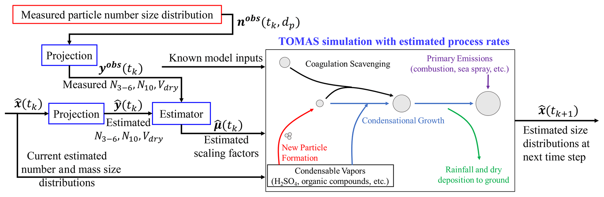
Figure 1Schematic of the TOMAS box model with the online estimation technique. The measured size distribution is projected to the inventory variables (N3–6, N10, Vdry), which the estimator compares to the current model prediction to calculate scaling factors that adjust particle formation, SOA production, and POA emission rates in TOMAS to simulate the size distribution with adjusted rates at the next time step.
2.2 Parameter estimation technique
To perform the inverse modeling technique, we adjust the TOMAS box model by introducing three time-varying scaling factors as the control variables that we want to estimate. Then, we estimate the control variables from moments of the size distribution that are sensitive to the uncertain processes. The estimation method used here requires us to define “inventory variables”, which are measurable quantities that are additive, positive, and continuously differentiable (McGuffin et al., 2019b). The observed and predicted size distributions are projected to the inventory variables (yk) at time tk, which are used to estimate the set of scaling factors input to TOMAS, as shown in Fig. 1. Here we choose to employ the following as inventory variables: (1) the particle concentration between 3 and 6 nm (N3–6), (2) the number concentration of particles greater than 10 nm (N10), (3) and the dry aerosol volume concentration (Vdry) (). These three variables are strongly sensitive to the uncertain processes of nucleation, emissions, and growth, respectively. The rates of change of the inventory variables depend on the scaling factors (μk) at time tk such that
where Gk is an array of the sensitivity of each inventory variable with respect to each uncertain process and fk is the vector of remaining terms in the inventory dynamics not directly dependent on the uncertain processes. Conceptually, Eq. (1) can be understood as a balance equation for the inventory variable, which is derived from the general dynamic equation for aerosol microphysics. For example, when yk corresponds to N10, the terms on the right consist of the rates of all the processes that add or remove particles from this size range. For N10, this would include the emission rates of any particles larger than 10 nm and growth of smaller particles to sizes larger than 10 nm in Gk, as well as formation or loss of particles in this size range by coagulation (in fk). Theoretically, they could be derived by a suitable integration of the aerosol general dynamic equation. In practice, in the code, Gk and are easily calculated online based on a backward finite-difference scheme since the model equations are solved using a forward-explicit Euler technique. Then, fk is determined from Eq. (1) based on the nominal scaling factor μk used to determine Gk. Because these rates are determined by finite difference, i.e., by saving model parameters before and after relevant subroutines are called, this approach is generalizable to various processes, modular, and robust with respect to changes in the aerosol microphysics. Internal details of subroutines can change so long as the estimator is able to compare the model state before and after the subroutine call. Additionally, this method can easily be adapted to other models with different uncertain processes or available measurements.
The parameter estimation technique was described in detail by McGuffin et al. (2019b); it was previously used to estimate sea spray emissions in a 3D CTM (McGuffin et al., 2019a). We will give a brief summary of the parameter estimation technique here. Instead of using a least-squares regression or the analytical maximum a posteriori solution, as other parameter estimates are generated (i.e., variational data assimilation or Bayesian inference techniques), we update the parameter estimate so that the model–measurement error exponentially decays, as shown in Eq. (2). In this case, the error is defined based on the chosen inventory variables (yk). The parameter estimate is calculated by solving the system of linear equations:
where is the model-predicted vector of inventory variables at time tk, is the observed vector of inventory variables, is the observed derivative of the vector of inventory variables, is the vector of estimated scaling factors, and Kc is a positive–definite diagonal array that determines the error exponential decay rate. Kc is analogous to a Kalman gain that weights the model–measurement bias. The gain has dimensions of frequency, i.e., inverse time. The gain determines how quickly the estimator forces the model to match the observations. High values of the gain accelerate convergence to observations. In contrast, decreasing the gain tends to weight the model more heavily than observations, increasing the time required for the model predictions to converge to observations so that the model does not follow the observations with high time resolution; the estimator will, however, reduce systematic biases if given sufficient time. This property of Kc allows the user to avoid noisy measurements corrupting the parameter estimates. For the rest of this paper, we use a matrix with diagonal elements of h−1 for Kc, which corresponds to convergence timescales of 15 min and 1 h for the number- and volume-based inventory variables, respectively. This array was found to have the best performance in reducing model–measurement mismatch without instabilities in the estimated scaling factors.
The left-hand side of Eq. (2) represents the rate of change of the model–measurement error, which is invertible for the scaling factors . The terms fk and Gk can be easily calculated online as described above. Because we require instantaneous sensitivity and model dynamics (Gk and fk), we must run the TOMAS algorithm twice for each time step (1) to determine fk and Gk from the nominal μk and (2) to move the simulation forward in time based on the estimated . The solution to the parameter estimation is implemented in the model in the second step to affect the complete number and mass size distributions.
There are two main drawbacks to the parameter estimation technique utilized here. First, we require knowledge of the derivative of the observations, which may include noise from differentiation. Unlike noise in the observations, noise in the derivatives cannot be dampened by adjusting the tuning parameter Kc. However, we can smooth to remove any differentiation noise with filtering techniques, such as the Savitzky–Golay filter. Second, Gk must have full rank and it should be well-conditioned to solve Eq. (2) for the scaling factors. If the sensitivity array is ill-conditioned, we cannot accurately solve the system of equations for the scaling factors to estimate the three process rates. This corresponds to the situation in which the measured inventory variables do not unambiguously constrain the process rates; i.e., several sets of process rates adequately satisfy the measured constraints, leaving at least two of the equations nearly linearly dependent. Physically, this can be thought of as a scenario in which inventory variables react to an aerosol process in the same way. For example, the system of equations using inventory variables N10 and N100 to estimate SOA production and emissions would be ill-conditioned in a scenario with the model predicting only particles greater than 100 nm and an emitted size distribution of particles 100 nm and larger. It follows that the condition number is not informed by any model–measurement mismatch.
We determine if the system is ill-conditioned based on the condition number (κ) of the relative sensitivity array (RSA), which is the element-wise product of the sensitivity array and the transpose of its inverse.
Here, the condition number is calculated as the ratio between the maximum and minimum eigenvalues of the square matrix (Highman, 2008), RSA, at time tk.
Another drawback of this estimation method, which is shared with most inverse techniques, is the effect of uncertainty in model errors not corrected by the estimator (fk uncertainty). Model errors outside of particle nucleation, emissions, and growth can lead the estimator to overcompensate in the scaling factors if the inventory variables are sensitive to those model errors. For example, the estimation technique applied to a model that does not correctly simulate particle deposition will estimate particle emissions incorrectly, while the estimated nucleation rate will not be affected. Identifying this scenario with outside model errors negatively impacting the estimated process rates is very difficult, but one sign is when the estimated process rates are not physical, e.g., a higher SOA production rate during nighttime. In future work, including various types of observations and more inventory variables can possibly inform the scaling factors and limit the impact of outside model errors on the estimated process rates.
Since the scaling factors are allowed to vary temporally, the estimated scaling factors are specific to the model and its a priori particle formation, emission, and growth rates. The scaling factors do not have any inherent physical meaning. Additionally, the estimated process rates cannot simply be reconstructed from the a priori rate and the estimated scaling factor since aerosol processes can be dependent on the state of the atmosphere; e.g., particle formation and growth depend on aerosol surface area. For all these reasons, instead of analyzing the estimated scaling factors, we will look at the estimated aerosol process rates.
2.3 Particle size distribution observations
The particle size distribution was observed from May 2006 through June 2007 at three rural locations: San Pietro Capofiume, Italy (SPC); Melpitz, Germany (MPZ); and the Station for Measuring Ecosystem–Atmosphere Relations II (Hari and Kulmala, 2005) site in Hyytiälä, Finland (HYY). All three measurement sites use twin-differential mobility particle sizer (DMPS) instruments to observe the ambient size distribution with particle diameters ranging from 3 nm to various upper size limits. The largest particle diameter measured is 0.6, 0.8, and 1 µm at SPC, MPZ, and HYY, respectively. The experimental setup at SPC and HYY was described by Aalto et al. (2001), and Birmili et al. (1999) described the setup at MPZ.
Random noise in the measured inventory variables could corrupt the estimated scaling factors. Instead of directly inputting the observed inventory variables, we smooth the observations and calculate their derivatives with a Savitzky–Golay filter (Savitzky and Golay, 1964). The filter fits a polynomial of a predetermined degree to the dataset over a time horizon that is also predetermined. The filtered value is then taken as the value of the polynomial at the midpoint of the time horizon. Additionally, the rate of change of a dataset is determined by differentiating the fitted polynomial at the midpoint. The method is computationally efficient since the there is an analytical solution to the best-fit polynomial coefficients (Savitzky and Golay, 1964).
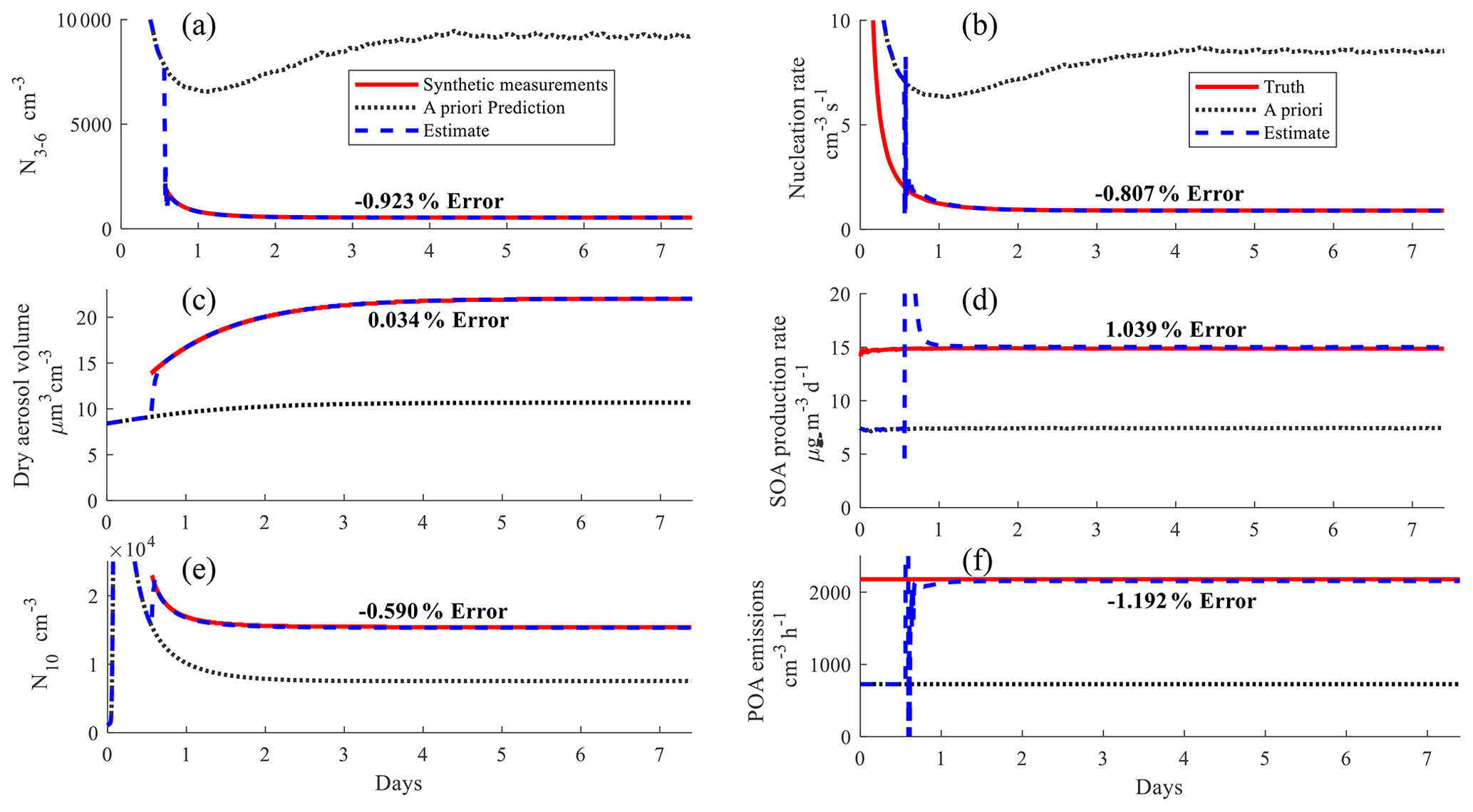
Figure 2Estimated, measured, and a priori inventory variables are in the left panels, and estimated, true, and a priori process rates are in the right panels for scenario no. 26 of the proof-of-concept scenarios. The measurements are (a) N3–6, (c) Vdry, and (e) N10. The process rates are (b) nucleation rate, (d) SOA production rate, and (f) POA emission rate.
In this work, we use the Savitzky–Golay filter of degree 1 so that we perform a moving-horizon average over a 3 h window on the raw measured inventory variables. A small averaging window is used for the field measurements to make sure the nucleation events are not filtered out. Then, we use finite differences on the filtered data to calculate the derivative of the measurements. The measurement derivatives and hourly filtered measurements are used to linearly interpolate the measurements to a frequency of 5 min, which is the model time step.
To evaluate the inverse modeling technique, we estimate particle formation, emissions, and growth rates based on simulated inventory variables, or “synthetic measurements”. The synthetic measurements are from the TOMAS box model itself with scaling factor inputs (μ*); the aerosol formation, emissions, and growth rates simulated are the so-called “true” rates. Then, TOMAS is run with the initial scaling factors at their nominal values (), but the inverse modeling technique adapts the scaling factors so the online model prediction matches the synthetic measurements. This configuration tests whether the estimation technique can recover the true process rates starting from a biased a priori model. This represents a best-case proof of concept because the synthetic measurements have no measurement noise and because the only errors in the a priori model are in the processes to be tuned. Nevertheless, it demonstrates the viability and potential performance of the theoretical approach. There is no outside noise included in the synthetic measurements and they are simulated with time-invariant scaling factors, but we apply a moving average with a 5 h window before utilizing in the inverse method to be consistent with the other simulations performed here.
Figure 2 shows how the inverse modeling approach performs for a week-long simulation in which the original model underpredicted aerosol mass (via dry aerosol volume Vdry) and N10, and it overpredicted the nucleation-mode number concentration (N3–6). Figure 2a, c, and e each show the a priori prediction if the scaling factors are not adjusted, the synthetic measurements, and the estimated inventory variables for N3–6, N10, and Vdry, respectively. Figure 2b, d, and f show the process rates for the a priori, the true values that determine the synthetic measurements, and the estimated rates of aerosol nucleation, emission, and SOA production, respectively. The first 12 h of the inverse modeling simulation is considered model spin-up, so the parameter estimation starts adjusting the scaling factors at t=12 h. We then evaluate the performance of the estimator starting at 24 h until the end of the simulation. The percent error between the average estimated and true value normalized by the average true value between days 1 and 7 for the aerosol measurements and rates is shown in each plot of Fig. 2. The method works very well in this case since the average bias for each measurement and aerosol process rate is less than 1 % and 2 %, respectively.

Figure 3Scatter plots of time-averaged (a) N3–6, (b) Vdry, and (c) N10 comparing the inverse modeling estimate and truth from synthetic measurements for each scenario. Circle and triangle markers represent well- and ill-conditioned scenarios, respectively. Open triangles represent scenarios unlikely to be observed with field measurements. The solid line is 1 : 1, and the dashed lines are 1 : 2 and 2 : 1.
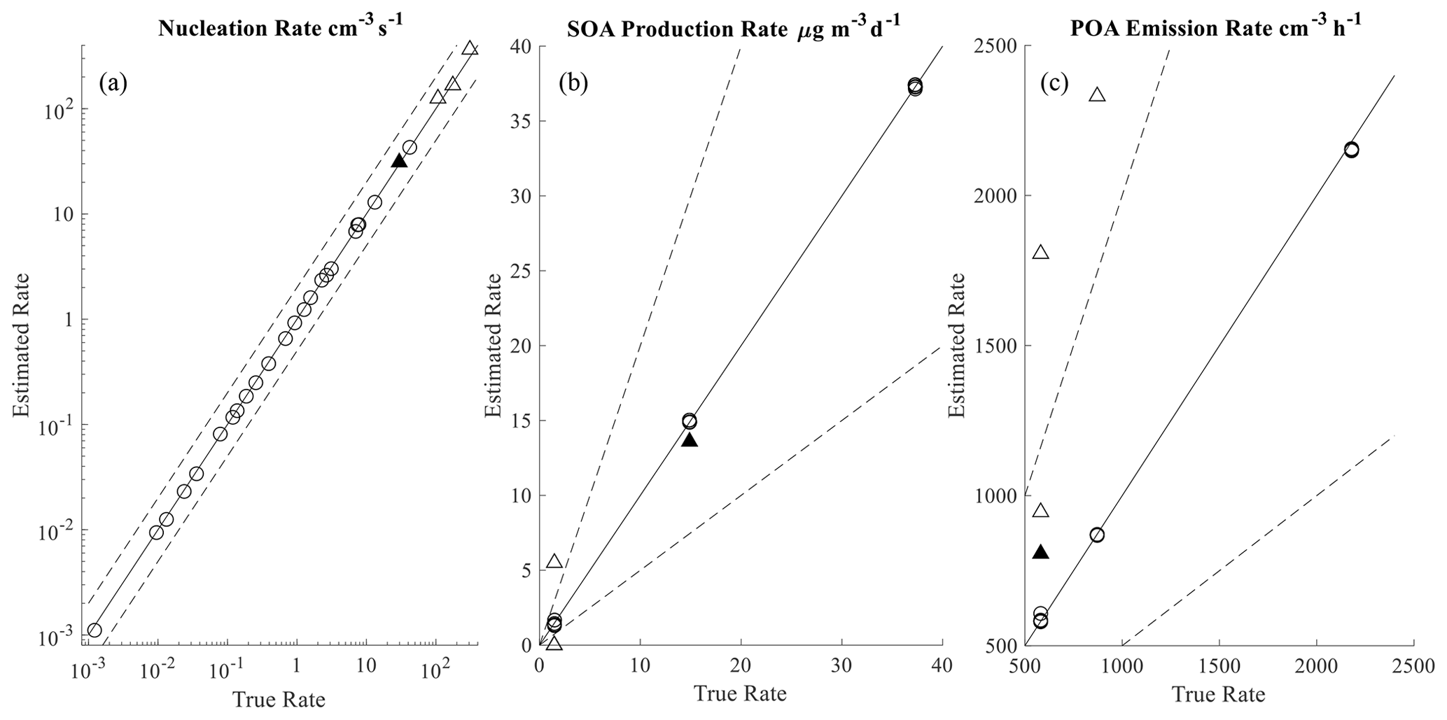
Figure 4Scatter plots of time-averaged nucleation rate (a), SOA production rate (b), and POA emission rate (c) comparing the inverse modeling estimate and truth for each scenario. See Fig. 3 for details.
Since the objective is to design an inverse technique that is robust enough to apply in a global 3D CTM, we repeat the above method for a set of 27 scenarios that span a range of process rates typically encountered in the atmosphere. We explore different particle formation, emissions, and SOA production rates that span approximately 0.001–300 cm−3 s−1, 580–2200 cm−3 h−1, and 1–38 µg m−3 d−1, respectively (Dunne et al., 2016; Fountoukis et al., 2012; Hodzic et al., 2016; Riemer et al., 2009). A weakness of this estimation method occurs when the sensitivity matrix (Gk) is ill-conditioned. Out of the 27 scenarios investigated here, four sets of synthetic measurements are deemed ill-conditioned as they were generated from a system in which the condition number, calculated with Eq. (3), is greater than 1.2 on average. In these cases, the condition number is near or equal to 1 for the majority of the simulation except for a small number of time steps in which the condition number spikes much higher, leading to an average condition number between 1.2 and 2.3. Common features among these ill-conditioned scenarios are very high nucleation rates coupled with low SOA production and low emission rates. Out of the four ill-conditioned scenarios, three scenarios were physically unrealistic in that they paired extremely high formation and extremely low growth rates – unlikely because the photochemistry that leads to nucleation events also tends to lead to high rates of condensational growth. Figure 3 shows the average estimate against the average measured inventory variables for all 27 scenarios. The only synthetic measurements that were not accurately estimated are ill-conditioned and unrealistic scenarios, which are denoted by the open triangle markers. The three inventory variables are estimated with an average error less than 11 % for the 23 well-conditioned scenarios and the one physically realistic ill-conditioned scenario.
Similarly, Fig. 4 shows that the estimated nucleation, emissions, and growth rates are accurately estimated if the synthetic measurements are well-conditioned. Particle formation only directly affects N3–6, which is significantly more sensitive to nucleation than emissions or growth, so we see that the nucleation rate is accurately estimated independent of the condition number. On the other hand, the accuracy of the estimated emissions and SOA production rates is strongly dependent on whether the true system is well-conditioned. Particle formation, emissions, and SOA production are each estimated with an average error less than 13 % in the 23 well-conditioned scenarios. In the worst-case scenario (the ill-conditioned but realistic scenario), aerosol nucleation, emissions, and SOA production rates are estimated with errors of 4 %, 38 %, and 9 % on average, respectively.
Although the inverse modeling technique in general estimates the correct inventory variables and aerosol process rates, we also wish to investigate whether the estimated size distribution will match the true size distribution. Accurately simulating the size distribution is very important to correctly predict the effect that aerosols have on climate. Figure 5 shows that the average estimated size distribution based on the inventory variables matches the average size distribution of the synthetic measurements generated from an intermediate set of particle formation, emissions, and SOA production rates. For the 23 well-conditioned scenarios with low bias in the estimated aerosol process rates, the estimated size distribution similarly closely matches the true size distribution.
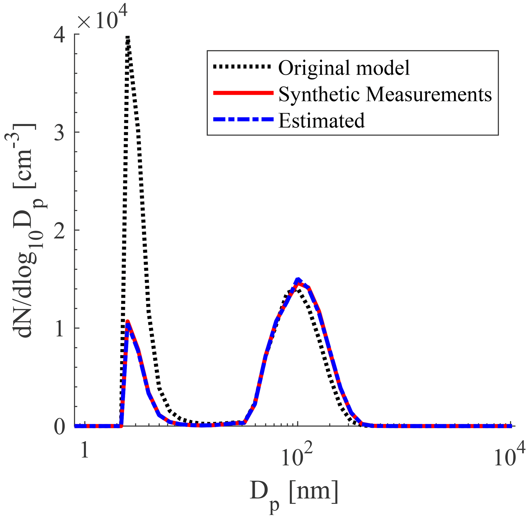
Figure 5Average particle size distributions in scenario no. 14 (nucleation, SOA production, POA emission rates: 2.7 cm−3 s−1, 15 µg m−3 d−1, 872 cm−3 h−1) from synthetic measurements, TOMAS run with a priori rates, and estimated with the inverse model are shown in the solid red, dotted black, and dashed blue profiles, respectively.
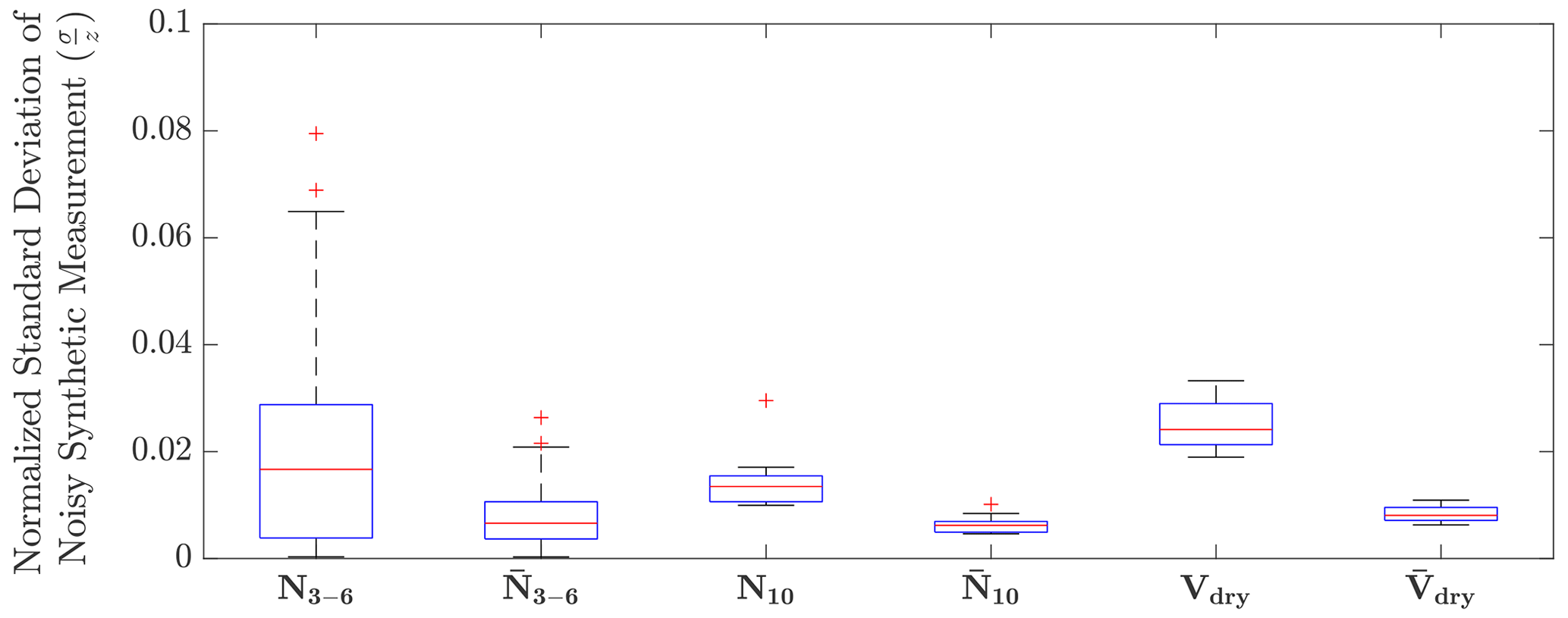
Figure 6Box plot showing the standard deviation of “noisy synthetic measurements” relative to their average value in all 27 scenarios for the inventory variables originally (N3–6, N10, Vdry) and after filtering (, , ).
Effect of measurement error on estimates
The estimation technique performs very well when utilizing “perfect measurements” (y*) that are not corrupted by any measurement noise or errors, but this is not a realistic scenario. We add noise to the 23 well-conditioned synthetic measurements explored in Sect. 3 to understand how measurement uncertainty will affect the estimated process rates. The noise added to each inventory variable is sampled, as random numbers, from a Gaussian probability distribution function with zero mean and a standard deviation of the approximated uncertainty in the respective inventory variable. The same set of random numbers is sampled for each scenario so that the noise signals in each of the 23 scenarios only vary in magnitude but their temporal profiles are the same.
We calculated the uncertainty in the size distribution from an instrument model described in Appendix A using the operating parameters of the DMPS operated at San Pietro Capofiume. The true size distribution is input to the instrument model to determine the size distribution uncertainty, which assumes Poisson counting statistics for each size bin from the counts by the condensation particle counter (Kangasluoma and Kontkanen, 2017). The inventory variables considered here are observed by combining several size bins observed by the DMPS. Inventory variable uncertainty is the uncertainty of the size distribution's corresponding size bins added in quadrature, which leads to inventory variables that are not as noisy as the individually measured particle sizes. Since the inventory variables are defined as the total concentration across a size range, the method intrinsically dampens instrument noise as random errors across multiple channels tend to cancel each other out.
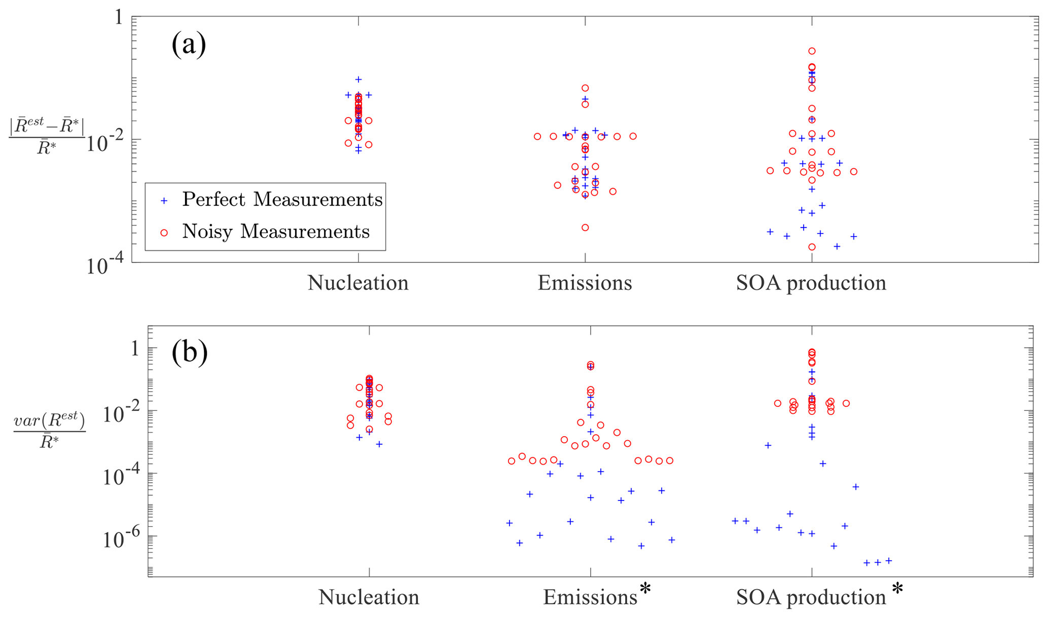
Figure 7Beeswarm plots showing (a) normalized mean error and (b) normalized variance in estimated nucleation, emissions, and SOA production rates (Rest) relative to the actual process rates (R*). The blue crosses show the 23 scenarios with perfect measurements, and the red circles show the same 23 scenarios with noisy measurements. * The difference between the perfect and noisy measurement scenarios is statistically significant for α=0.05.
The normalized standard deviation in the noisy N3–6, N10, and Vdry (with respect to their average value with noise) across the 27 scenarios is less than 0.08, 0.03, and 0.04, respectively. Then, we filter the synthetic noisy measurements with an 11 h window and a first-degree polynomial with the Savitzky–Golay filter to produce measurement values and derivatives that are smooth. As shown in Fig. 6, the relative standard deviation of each inventory variable decreases to less than 0.03, 0.011, and 0.011 for N3–6, N10, and Vdry, respectively. The filtered noisy synthetic measurements and their derivatives were used to estimate particle formation, emissions, and SOA production in the same 27 scenarios that were investigated in the previous section. Since we observe poor performance in 4 ill-conditioned scenarios, we focus on the remaining 23 well-conditioned scenarios in this section. The same version of TOMAS that was used above is used here, and the same estimation algorithm is used except for additional code to handle the scenario when the system of equations is ill-conditioned. At each time step, we evaluate the condition number of the system of equations as in Eq. (3) within the estimation algorithm; if its value is greater than 3, the equation and unknown scaling factor corresponding to the row with the largest eigenvalue are removed. This corresponds to solving for just two uncertain process rates instead of three. When a scaling factor is removed from the system of equations, it then is assigned its value from the previous time step.
Figure 7 shows the mean bias and variance in the estimated process rates for each of the 23 scenarios as blue crosses and red circles when synthetic measurements without and with noise are used, respectively. In Fig. 7a, we find that the normalized mean bias across the 23 scenarios does not significantly change, with median values without and with noise of 0.03 and 0.03, 0.005 and 0.007, and 0.004 and 0.006 for nucleation, emissions, and growth, respectively. Figure 7b shows a statistically significant difference in the normalized variance of estimated SOA production and POA emission rates between the cases using measurements with and without noise. The estimated process rates using noisy measurements have a somewhat higher variance compared to the estimates with perfect measurements. The high variance in estimated process rates is due to the estimator tracking synthetic measurement noise, which is translated to noise in the process rates. In the future, the gain should be adjusted to a lower value so the measurement noise is filtered and the estimated process rates are smoother.
This section evaluates the inverse method by utilizing field measurements of particle size distribution from SPC, MPZ, and HYY instead of synthetic measurements to estimate particle formation, emissions, and SOA production. Since we previously found that an ill-conditioned sensitivity matrix results in inaccurately estimated process rates when using synthetic measurements, we avoid solving an ill-conditioned system by reducing the system of equations. If the condition number of Gk is greater than a threshold of 5, then we assume that the scaling factor for SOA production is constant from the previous time step and estimate the other two scaling factors based on N3–6 and N10 inventory variables. Here, we eliminate the equation for Vdry and eliminate the unknown scaling factor on SOA production as we observed that the full system of equations is ill-conditioned because N10 and Vdry are very close to co-linear. Since N10 is more directly measured than Vdry, we choose to remove Vdry.
The purpose of this section is to test the inverse method on real data, including size distributions not generated by the TOMAS model itself (the synthetic measurements above). A challenge here arises from the processes that are not well-captured in a box modeling framework, namely long-range transport of aerosol to the measurement site, including abrupt changes in air mass. Recognizing that our long-term goal is to deploy the estimation framework in a three-dimensional model that will include an improved and more detailed representation of long-range transport, we mitigate them here with several simple approaches.
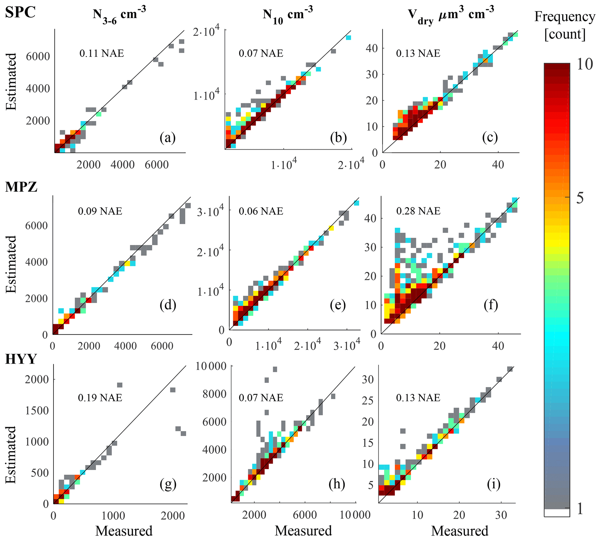
Figure 8Frequency scatter plots comparing hourly estimates to hourly measurements of N3–6, N10, and Vdry in the first, second, and third columns, respectively. Measurements from San Pietro Capofiume, Melpitz, and Hyytiälä are shown in the first, second, and third rows, respectively. The black line shows the 1 : 1 line. Normalized absolute error (NAE) is shown at the top of each panel.
First, we filter the measurements to select time periods when meteorology is relatively stable. We classify whether a time is stagnant from the three conditions determined by Garrido-Perez et al. (2018) in addition to a condition on the sea level pressure. A time period is considered stagnant if (1) the reanalysis wind speed at 10 m of altitude is less than 3.2 m s−1, (2) the reanalysis wind speed at 500 hPa is less than 13 m s−1, (3) daily precipitation is less than 1 mm, and (4) sea level pressure is greater than 1020 hPa. The reanalysis precipitation fields are retrieved from the European Climate Assessment & Dataset E-OBS at a resolution of 0.25∘ latitude by 0.25∘ longitude (Cornes et al., 2018), while wind speed and sea level pressure are from the National Aeronautics and Space Administration's MERRA-2 at 0.5∘ latitude by 0.625∘ longitude. All of the conditions must be met for at least 24 h before the remaining hours fulfilling the constraints are considered stable. These conditions leave us with 23, 31, and 18 d out of the 1 year of measurements at SPC, MPZ, and HYY, respectively. Out of the filtered measurements at each site, 24 %, 43 %, and 41 % are from the spring season in SPC, MPZ, and HYY, respectively.
Second, we choose a first-order removal timescale that is faster than aerosol removal processes (i.e., deposition) to allow the box model to adjust to air mass changes. Finally, we use this largely as a proof of concept, taking caution in interpreting the process rates. We expect that, in a box modeling framework, the N3–6 inventory variable and nucleation rates will be the most realistic of the process variables since nucleation-mode particles are short-lived, and long-range transport is a relatively minor factor in determining their concentrations. In contrast, we do not seek to interpret the emissions or SOA production rates since the inverse model will naturally adjust them artificially to compensate for transport processes not represented in the box model. Therefore, for this work, we further simplify the box model as described in the next section.
4.1 Simulating ambient aerosol with TOMAS
The inverse modeling method assumes that all simulated processes in the box model are correct except for the processes scaled by the control variables. Thus, the primary emitted size distribution must have the correct shape in order to estimate emissions correctly. The aerosol size distribution we emit into the TOMAS box model in this section reflects primary organic aerosol emissions from a 3D CTM (GEOS-Chem). Here, the particle emissions are from fossil fuel and biomass burning emission inventories averaged over western Europe (Bond et al., 2007).
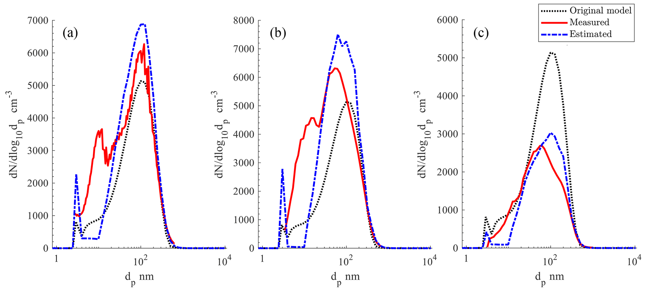
Figure 9Average particle size distributions measured, originally predicted with a priori rates in TOMAS, and estimated with the inverse model are shown in the solid red, dotted black, and dashed blue profiles, respectively. Results are shown using measurements at (a) San Pietro Capofiume, (b) Melpitz, and (c) Hyytiälä.
Additionally, we remove condensation of sulfuric acid from the box model simulation so that we are estimating overall particle growth while perturbing SOA production with the growth scaling factor. Using only this box model and measurements of particle size distribution, we cannot distinguish between sulfate and VOC condensation since both similarly affect the size distribution in the model. Since we have removed sulfuric acid from the box model, the default nucleation parameterization will not produce new particles. Instead, we replace the nucleation scheme with a constant new particle formation rate of 0.2 cm−3 s−1. This will only affect the estimated scaling factors and not the estimated nucleation rates.
4.2 Estimation results
At each measurement site, the estimated inventory variables are close to the hourly measurement of those same parameters, as shown in Fig. 8. At SPC, MPZ, and HYY the normalized absolute errors across the three inventory variables are 0.10, 0.14, and 0.13, respectively, which is improved with respect to the predictions with a priori process rates, as shown in Fig. S1 in the Supplement. Each row in Fig. 8 shows frequency scatter plots of the hourly estimated versus observed inventory variable; the color represents the count of data points in that respective grid cell.
Figure 9 shows the average estimated, measured, and original model-predicted size distributions at each measurement site. Although the inventory variables are close to the observations, the estimated size distributions do not match as well as with the synthetic measurements. We expect that the estimated size distribution does not match the field measurements because the mass and number of particles larger than 100 nm indicate long-range species that are influenced by processes not included in the version of TOMAS used here, i.e., various primary aerosol emission sources, transport, aerosol aging. Several factors contribute to the bias between the estimated and observed size distribution between 4 and 20 nm. First, TOMAS nucleates 3 nm particles based on the N3–6 measurement in order to match the total number concentration in the 3 to 6 nm range to the observations, but the shape of the size distribution within that range does not match since all new particles enter through the 3 nm size bin. Second, the estimated SOA production rates exhibit similar high variability as the estimated nucleation rate in order to account for changes in air mass and wind direction not included in the model. Since peaks in the estimated growth from SOA production do not always coincide with nucleation events, the model simulation forms the two distinct modes at 3 and 100 nm, as shown in Fig. 9.
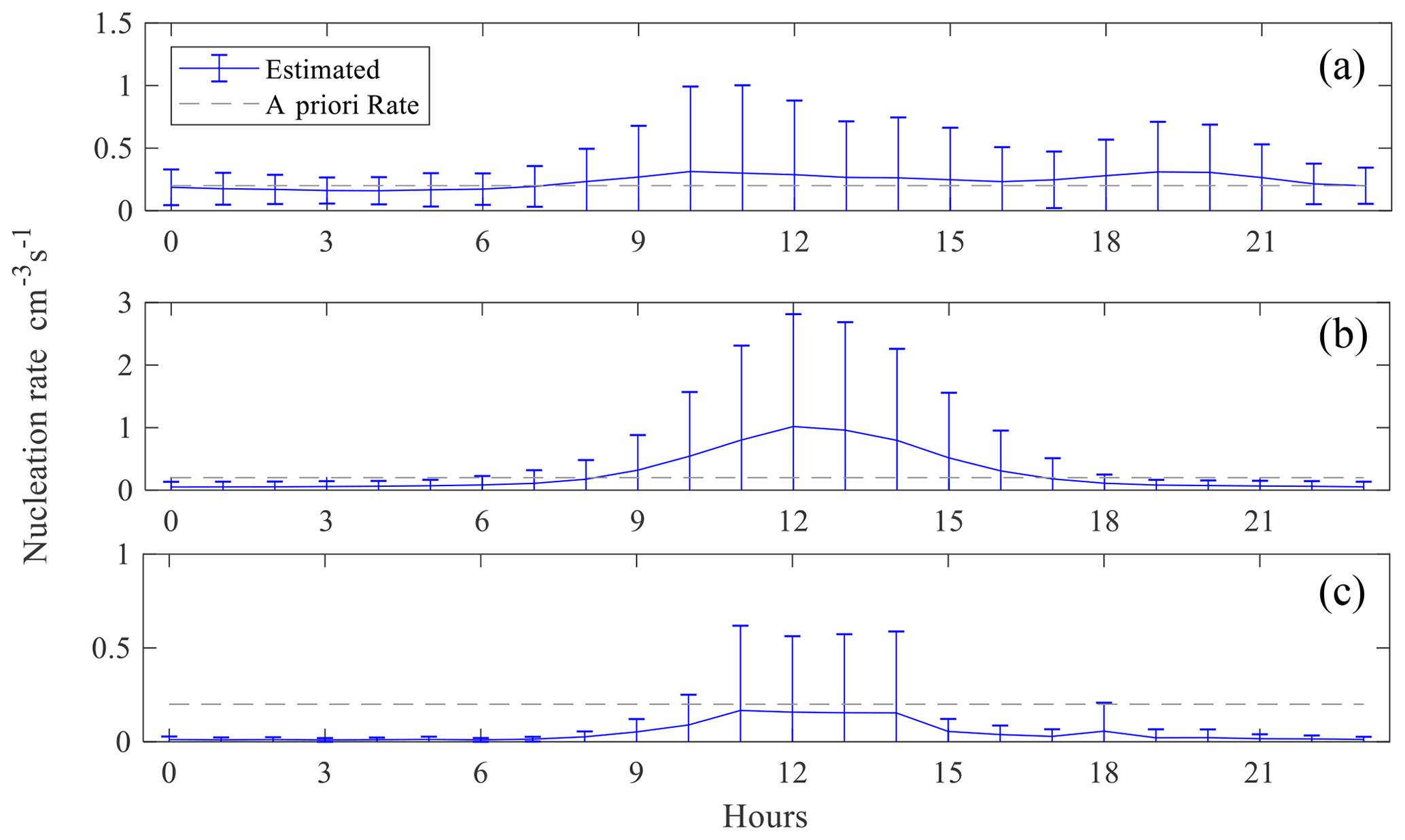
Figure 10Estimated diurnal nucleation rate during stagnant events for each measurement site: (a) San Pietro Capofiume, (b) Melpitz, (c) Hyytiälä. Blue solid and grey dashed lines show the estimated rate and a priori rate, respectively; the error bars show the standard deviation across all days.
We find that the estimated nucleation rates are reasonable as shown in Fig. 10, which shows the average diurnal profile estimated for each site. The average estimated nucleation rate at all of the sites has a realistic magnitude near 1 cm−3 s−1, which agrees with previous simulation results at HYY (Kulmala et al., 2005; Westervelt et al., 2014). MPZ and HYY have a clear peak in particle formation near noon local time, correlating with photochemical production of condensable vapors. At HYY we see an increase in estimated particle formation rate at 18:00 local time, which occurs after sunset on 22 February and before sunset on 28 March. The estimated diurnal profile of formation at SPC includes significant formation, even during nighttime. To understand the large, fairly consistent nucleation rate at SPC, we can examine the average diurnal profile of the measured N3–6, as shown in Fig. S3. The fairly constant N3–6 measurement throughout the day may indicate an instrument bias, which introduces a similar bias into the estimated nucleation rate at SPC.
This work has explored a way to assimilate particle size distribution data with an aerosol microphysics algorithm used in 3D CTMs by designing a novel estimation algorithm borrowed from the field of nonlinear process control. The estimation framework is robust, computationally inexpensive, and flexible to model updates. It has been tested with synthetic measurements, noisy synthetic measurements, and European field measurements. We show that the particle size distribution inverse modeling technique estimates particle formation, emissions, and SOA production accurately when there is no measurement error and all other processes are known accurately. N3–6, N10, and Vdry are estimated within 11 % error of the synthetic measurements across 24 realistic scenarios that span global conditions. New particle formation, emissions, and growth rates were estimated within 13 % of the true rates in 23 scenarios that are well-conditioned. Moreover, the estimated size distribution matches the synthetic measurements when the inventory variables are accurately estimated. Introducing realistic instrumental noise into the synthetic measurements results in a statistically significant increase in the variance of the estimated SOA production and emission rates. Nonetheless, no significant biases were introduced in the estimated process rates across the 23 well-conditioned scenarios when adding noise to the synthetic measurements.
We applied the inverse technique to field data from San Pietro Capofiume, Melpitz, and Hyytiälä between May 2006 and June 2007. Error in the estimated N3–6, N10, and Vdry is less than 15 % during stagnant measurement days for which the meteorology is most amenable to a box modeling framework. Although the estimated emissions and growth are not necessarily accurate since the box model cannot represent long-range transport of aerosol resulting from these processes, we can estimate the nucleation rate. The average estimated nucleation rates at Melpitz and Hyytiälä have peaks near noon local time with average values of 1 and 0.15 cm−3 s−1, respectively. This application demonstrates the ability of our method to derive reasonable process rates from long-term aerosol size distribution measurements.
Although there is reason to believe that the estimated emissions and SOA production rates are not correct when applying the box model to field measurements, these rates are estimated correctly in the synthetic measurement case. The key differences between field and synthetic measurements are the model–measurement biases outside of particle formation, emissions, and growth. The zero-dimensional version of TOMAS used here does not incorporate sufficient detail about meteorology or emission sources to give successful inverse modeling results. However, a 3D CTM that includes processes such as transport, photochemistry, and diverse emission sources could be more successful in an inverse modeling study. If the method applied here is integrated into a 3D CTM, there is potential to estimate key uncertain parameters that control aerosol dynamics and thereby improve the predicted size distribution field.
The DMPS takes aerosol samples and reports the particle count of a specific size bin during a time interval, as represented by the following equation:
where represents the counts of particles in each size bin, is the actual particle size distribution, and M is the matrix involving all the processes inside the DMPS (Pfeifer et al., 2014): the charging probability, the transfer function, and the counting efficiency of the detector. The charging probability follows the empirical approximation by Wiedensohler (1988). For a specific voltage, flow rates, and the geometry of the differential mobility analyzer (DMA), the DMPS system is at steady state, so the Stolzenburg (1988) transfer function can be used to approximate the transmission efficiency of particles at the corresponding conditions. The counting efficiency of the detector is determined by the parameters from Mertes (1995).
We assume that the uncertainty of the measurement only comes from the counting, which follows Poisson counting statistics, since the information about the uncertainty of the working conditions is unknown. Thus, the uncertainty from measurement is , which yields the uncertainty of the particle size distribution, En, as follows.
The model generates the matrix M, and with the input of the actual particle size distribution n, it first calculates the counts c and its element-wise square root (); then it applies the totally nonnegative least-squares method (Merritt and Zhang, 2005) to obtain the uncertainty of the particle size distribution En.
The code used in this work is available online (McGuffin, 2020). Data on particle size distribution measurements were provided through the EBAS (Aalto and Kulmala, 2012; Sonntag et al., 2008) for the MPZ and HYY stations. Stefano Decesari provided size distribution measurements for the SPC station. Precipitation data were downloaded from the European Climate Assessment & Dataset (Cornes et al., 2018). Sea level pressure and wind speed data were downloaded from the NASA Goddard Earth Sciences Data and Information Center (GMAO, 2015a, b).
The supplement related to this article is available online at: https://doi.org/10.5194/gmd-14-1821-2021-supplement.
PJA, BEY, and DLM conceptualized the simulations and estimation technique. DLM adapted the model code with the estimation algorithm and performed all simulations. RF and YH conceptualized the measurement uncertainty. YH created the uncertainty code. DLM authored the text with contributions from all co-authors. YH wrote Appendix A.
The authors declare that they have no conflict of interest.
The authors acknowledge Thomas Tuch, Pasi Aalto, Stefano Decesari, and Jorma Joutsensaari for providing descriptions and technical specifications of their measurement setup. This work was performed partially under the auspices of the US Department of Energy by the Lawrence Livermore National Laboratory under contract DE-AC52-07NA27344 with IM release number LLNL-JRNL-813683.
We acknowledge the E-OBS dataset from the EU-FP6 project UERRA (http://www.uerra.eu, last access: 24 March 2021) and the data providers in the ECA&D project (https://www.ecad.eu, last access: 24 March 2021).
This research was supported by the Carnegie Mellon University Department of Chemical Engineering and the Mahmood I. Bhutta Fellowship in Chemical Engineering. Tuukka Petäjä acknowledges financial support through the Academy of Finland (304347), the Center of Excellence in Atmospheric Sciences, and the European Commission through the Horizon 2020 research and innovation program under grant agreement no. 689443 via project iCUPE (Integrative and Comprehensive Understanding on Polar Environments).
This paper was edited by Christina McCluskey and reviewed by three anonymous referees.
Aalto, P., Hämeri, K., Becker, E., Weber, R., Salm, J., Mäkelä, J. M., Hoell, C., O'dowd, C. D., Hansson, H.-C., Väkevä, M., Koponen, I. K., Buzorius, G., and Kulmala, M.: Physical characterization of aerosol particles during nucleation events, Tellus B, 53, 344–358, https://doi.org/10.3402/tellusb.v53i4.17127, 2001.
Aalto, P. and Kulmala, M.: Finland – Hyytiälä (FI0050R) – dmps – particle_number_size_distribution – aerosol [data set], available at: http://ebas.nilu.no/DataSets.aspx?stations=FI0050R&InstrumentTypes=dmps&components=particle_number_size_distribution&fromDate=1970-01-01&toDate=2021-12-31 (last access: 24 March 2021), 2012.
Adams, P. J. and Seinfeld, J. H.: Predicting global aerosol size distributions in general circulation models, J. Geophys. Res.-Atmos., 107, AAC 4-1–AAC 4-23, https://doi.org/10.1029/2001JD001010, 2002.
Adams, P. J., Donahue, N. M., and Pandis, S. N.: Atmospheric nanoparticles and climate change, AIChE J., 59, 4006–4019, https://doi.org/10.1002/aic.14242, 2013.
Asmi, A., Wiedensohler, A., Laj, P., Fjaeraa, A.-M., Sellegri, K., Birmili, W., Weingartner, E., Baltensperger, U., Zdimal, V., Zikova, N., Putaud, J.-P., Marinoni, A., Tunved, P., Hansson, H.-C., Fiebig, M., Kivekäs, N., Lihavainen, H., Asmi, E., Ulevicius, V., Aalto, P. P., Swietlicki, E., Kristensson, A., Mihalopoulos, N., Kalivitis, N., Kalapov, I., Kiss, G., de Leeuw, G., Henzing, B., Harrison, R. M., Beddows, D., O'Dowd, C., Jennings, S. G., Flentje, H., Weinhold, K., Meinhardt, F., Ries, L., and Kulmala, M.: Number size distributions and seasonality of submicron particles in Europe 2008–2009, Atmos. Chem. Phys., 11, 5505–5538, https://doi.org/10.5194/acp-11-5505-2011, 2011.
Balaji, S., Du, J., White, C. M., and Ydstie, B. E.: Multi-scale modeling and control of fluidized beds for the production of solar grade silicon, Powder Technol., 199, 23–31, https://doi.org/10.1016/j.powtec.2009.04.022, 2010.
Ban-Weiss, G. A., Lunden, M. M., Kirchstetter, T. W., and Harley, R. A.: Size-resolved particle number and volume emission factors for on-road gasoline and diesel motor vehicles, J. Aerosol Sci., 41, 5–12, https://doi.org/10.1016/j.jaerosci.2009.08.001, 2010.
Benedetti, A., Reid, J. S., Knippertz, P., Marsham, J. H., Di Giuseppe, F., Rémy, S., Basart, S., Boucher, O., Brooks, I. M., Menut, L., Mona, L., Laj, P., Pappalardo, G., Wiedensohler, A., Baklanov, A., Brooks, M., Colarco, P. R., Cuevas, E., da Silva, A., Escribano, J., Flemming, J., Huneeus, N., Jorba, O., Kazadzis, S., Kinne, S., Popp, T., Quinn, P. K., Sekiyama, T. T., Tanaka, T., and Terradellas, E.: Status and future of numerical atmospheric aerosol prediction with a focus on data requirements, Atmos. Chem. Phys., 18, 10615–10643, https://doi.org/10.5194/acp-18-10615-2018, 2018.
Bergamaschi, P., Krol, M., Meirink, J. F., Dentener, F., Segers, A., Van Aardenne, J., Monni, S., Vermeulen, A. T., Schmidt, M., Ramonet, M., Yver, C., Meinhardt, F., Nisbet, E. G., Fisher, R. E., O'Doherty, S., and Dlugokencky, E. J.: Inverse modeling of European CH4 emissions 2001–2006, J. Geophys. Res.-Atmos., 115, D22309, https://doi.org/10.1029/2010JD014180, 2010.
Birmili, W., Stratmann, F., and Wiedensohler, A.: Design of a DMA-Based size spectrometer for a large particle size range and stable operation, J. Aerosol. Sci., 30, 549–553, 1999.
Birmili, W., Sun, J., Weinhold, K., Merkel, M., Rasch, F., Spindler, G., Wiedensohler, A., Bastian, S., Löschau, G., Schladitz, A., Quass, U., Kuhlbusch, T. A. J., Kaminski, H., Cyrys, J., Pitz, M., Gu, J., Peters, A., Flentje, H., Meinhardt, F., Schwerin, A., Bath, O., Ries, L., Gerwig, H., Wirtz, K., and Weber, S.: Atmospheric aerosol measurements in the German Ultrafine Aerosol Network (GUAN), Aerosolmessung Gefahrstoffe–Reinhaltung der Luft, 7512(11), 2015.
Bond, T. C., Bhardwaj, E., Dong, R., Jogani, R., Jung, S., Roden, C., Streets, D. G., and Trautmann, N. M.: Historical emissions of black and organic carbon aerosol from energy-related combustion, 1850–2000, Global Biogeochem. Cy., 21, GB2018, https://doi.org/10.1029/2006GB002840, 2007.
Carslaw, K. S., Lee, L. A, Reddington, C. L., Pringle, K. J., Rap, A., Forster, P. M., Mann, G. W., Spracklen, D. V., Woodhouse, M. T., Regayre, L. A., and Pierce, J. R.: Large contribution of natural aerosols to uncertainty in indirect forcing, Nature, 503, 67–71, https://doi.org/10.1038/nature12674, 2013.
Chen, C., Dubovik, O., Henze, D. K., Chin, M., Lapyonok, T., Schuster, G. L., Ducos, F., Fuertes, D., Litvinov, P., Li, L., Lopatin, A., Hu, Q., and Torres, B.: Constraining global aerosol emissions using POLDER/PARASOL satellite remote sensing observations, Atmos. Chem. Phys., 19, 14585–14606, https://doi.org/10.5194/acp-19-14585-2019, 2019.
Cornes, R. C., van der Schrier, G., van den Besselaar, E. J. M., and Jones, P. D.: An Ensemble Version of the E-OBS Temperature and Precipitation Data Sets, J. Geophys. Res.-Atmos., 123, 9391–9409, https://doi.org/10.1029/2017JD028200, 2018.
Cubasch, U. D., Chen, D., Facchini, M. C., Frame, D., Mahowald, N. and Winther, J. G.: Climate Change 2013: The Physical Science Basis. Contribution of Working Group I to the Fifth Assessment Report of the Intergovernmental Panel on Climate Change, edited by: Stocker, T. F., Qin, D., Plattner, G. K., Tignor, M., Allen, S. K., Boschung, J., Nauels, A., Xia, Y., Bex, V., and Midgley, P. M., Cambridge University Press, 2013.
Dubovik, O., Lapyonok, T., Kaufman, Y. J., Chin, M., Ginoux, P., Kahn, R. A., and Sinyuk, A.: Retrieving global aerosol sources from satellites using inverse modeling, Atmos. Chem. Phys., 8, 209–250, https://doi.org/10.5194/acp-8-209-2008, 2008.
Dunne, E. M., Gordon, H., Kürten, A., Almeida, J., Duplissy, J., Williamson, C., Ortega, I. K., Pringle, K. J., Adamov, A., Baltensperger, U., Barmet, P., Benduhn, F., Bianchi, F., Breitenlechner, M., Clarke, A., Curtius, J., Dommen, J., Donahue, N. M., Ehrhart, S., Flagan, R. C., Franchin, A., Guida, R., Hakala, J., Hansel, A., Heinritzi, M., Jokinen, T., Kangasluoma, J., Kirkby, J., Kulmala, M., Kupc, A., Lawler, M. J., Lehtipalo, K., Makhmutov, V., Mann, G., Mathot, S., Merikanto, J., Miettinen, P., Nenes, A., Onnela, A., Rap, A., Reddington, C. L. S., Riccobono, F., Richards, N. A. D., Rissanen, M. P., Rondo, L., Sarnela, N., Schobesberger, S., Sengupta, K., Simon, M., Sipilä, M., Smith, J. N., Stozkhov, Y., Tomé, A., Tröstl, J., Wagner, P. E., Wimmer, D., Winkler, P. M., Worsnop, D. R., and Carslaw, K. S.: Global atmospheric particle formation from CERN CLOUD measurements, Science, 354, 1119–1124, https://doi.org/10.1126/science.aaf2649, 2016.
Easter, R. C.: MIRAGE: Model description and evaluation of aerosols and trace gases, J. Geophys. Res., 109, D20210, https://doi.org/10.1029/2004JD004571, 2004.
Escribano, J., Boucher, O., Chevallier, F. and Huneeus, N.: Subregional inversion of North African dust sources, J. Geophys. Res.-Atmos., 121, 8549–8566, https://doi.org/10.1002/2016JD025020, 2016.
Escribano, J., Boucher, O., Chevallier, F., and Huneeus, N.: Impact of the choice of the satellite aerosol optical depth product in a sub-regional dust emission inversion, Atmos. Chem. Phys., 17, 7111–7126, https://doi.org/10.5194/acp-17-7111-2017, 2017.
Farschman, C. A., Viswanath, K. P., and Erik Ydstie, B.: Process systems and inventory control, AIChE J., 44, 1841–1857, https://doi.org/10.1002/aic.690440814, 1998.
Folberth, G. A., Hauglustaine, D. A., Lathière, J., and Brocheton, F.: Interactive chemistry in the Laboratoire de Météorologie Dynamique general circulation model: model description and impact analysis of biogenic hydrocarbons on tropospheric chemistry, Atmos. Chem. Phys., 6, 2273–2319, https://doi.org/10.5194/acp-6-2273-2006, 2006.
Fountoukis, C., Riipinen, I., Denier van der Gon, H. A. C., Charalampidis, P. E., Pilinis, C., Wiedensohler, A., O'Dowd, C., Putaud, J. P., Moerman, M., and Pandis, S. N.: Simulating ultrafine particle formation in Europe using a regional CTM: contribution of primary emissions versus secondary formation to aerosol number concentrations, Atmos. Chem. Phys., 12, 8663–8677, https://doi.org/10.5194/acp-12-8663-2012, 2012.
Garrido-Perez, J. M., Ordóñez, C., García-Herrera, R., and Barriopedro, D.: Air stagnation in Europe: Spatiotemporal variability and impact on air quality, Sci. Total Environ., 645, 1238–1252, https://doi.org/10.1016/j.scitotenv.2018.07.238, 2018.
Gilliland, A. B., Dennis, R. L., Roselle, S. J., and Pierce, T. E.: Seasonal NH3 emission estimates for the eastern United States based on ammonium wet concentrations and an inverse modeling method, J. Geophys. Res., 108, 4477, https://doi.org/10.1029/2002JD003063, 2003.
Global Modeling and Assimilation Office (GMAO): MERRA-2 tavg1_2d_slv_Nx: 2d,1-Hourly,Time-Averaged,Single-Level,Assimilation,Single-Level Diagnostics V5.12.4, Greenbelt, MD, USA, Goddard Earth Sciences Data and Information Services Center (GES DISC), https://doi.org/10.5067/VJAFPLI1CSIV (last access: 1 May 2018), 2015a.
Global Modeling and Assimilation Office (GMAO): MERRA-2 tavg3_3d_asm_Nv: 3d,3-Hourly,Time-Averaged,Model-Level,Assimilation,Assimilated Meteorological Fields V5.12.4, Greenbelt, MD, USA, Goddard Earth Sciences Data and Information Services Center (GES DISC), https://doi.org/10.5067/SUOQESM06LPK (last access: 1 May 2018), 2015b.
Hari, P. and Kulmala, M.: Station for Measuring Ecosystem-Atmosphere Relations (SMEAR II), Boreal Environ. Res., 10, 315–322, 2005.
Hein, R., Crutzen, P. J., and Heimann, M.: An inverse modeling approach to investigate the global atmospheric methane cycle, Global Biogeochem. Cy., 11, 43–76, 1997.
Henze, D. K., Seinfeld, J. H., and Shindell, D. T.: Inverse modeling and mapping US air quality influences of inorganic PM2.5 precursor emissions using the adjoint of GEOS-Chem, Atmos. Chem. Phys., 9, 5877–5903, https://doi.org/10.5194/acp-9-5877-2009, 2009.
Highman, N. J.: Conditioning, in: Functions of Matrices (Environmental Engineering), Society for Industrial and Applied Mathematics, 55–70, https://doi.org/10.1137/1.9780898717778.ch3, 2008.
Hodzic, A., Kasibhatla, P. S., Jo, D. S., Cappa, C. D., Jimenez, J. L., Madronich, S., and Park, R. J.: Rethinking the global secondary organic aerosol (SOA) budget: stronger production, faster removal, shorter lifetime, Atmos. Chem. Phys., 16, 7917–7941, https://doi.org/10.5194/acp-16-7917-2016, 2016.
Houweling, S., Kaminski, T., Dentener, F., Lelieveld, J., and Heimann, M.: Inverse modeling of methane sources and sinks using the adjoint of a global transport model Sander global methane emissions, J. Geophys. Res., 104, 26137–26160, https://doi.org/10.1029/1999JD900428, 1999.
Huneeus, N., Chevallier, F., and Boucher, O.: Estimating aerosol emissions by assimilating observed aerosol optical depth in a global aerosol model, Atmos. Chem. Phys., 12, 4585–4606, https://doi.org/10.5194/acp-12-4585-2012, 2012.
Huneeus, N., Boucher, O., and Chevallier, F.: Atmospheric inversion of SO2 and primary aerosol emissions for the year 2010, Atmos. Chem. Phys., 13, 6555–6573, https://doi.org/10.5194/acp-13-6555-2013, 2013.
Kajino, M. and Kondo, Y.: EMTACS: Development and regional-scale simulation of a size, chemical, mixing type, and soot shape resolved atmospheric particle model, J. Geophys. Res.-Atmos., 116, D02303, https://doi.org/10.1029/2010JD015030, 2011.
Kangasluoma, J. and Kontkanen, J.: On the sources of uncertainty in the sub-3 nm particle concentration measurement, J. Aerosol Sci., 112, 34–51, https://doi.org/10.1016/j.jaerosci.2017.07.002, 2017.
Kerminen, V. M., Chen, X., Vakkari, V., Petäjä, T., Kulmala, M., and Bianchi, F.: Atmospheric new particle formation and growth: Review of field observations, Environ. Res. Lett., 13, 103003, https://doi.org/10.1088/1748-9326/aadf3c, 2018.
Kulmala, M., Petäjä, T., Mönkkönen, P., Koponen, I. K., Dal Maso, M., Aalto, P. P., Lehtinen, K. E. J., and Kerminen, V.-M.: On the growth of nucleation mode particles: source rates of condensable vapor in polluted and clean environments, Atmos. Chem. Phys., 5, 409–416, https://doi.org/10.5194/acp-5-409-2005, 2005.
Kulmala, M., Pet, T., Nieminen, T., Sipil, M., Manninen, H. E., Lehtipalo, K., Dal Maso, M., Aalto, P. P., Junninen, H., Paasonen, P., Riipinen, I. J., Lehtinen, K. E., Laaksonen, A., and Kerminen, V.-M.: Measurement of the nucleation of atmospheric aerosol particles, Nat. Protoc., 7, 1651–1667, https://doi.org/10.1038/nprot.2012.091, 2012.
Kulmala, M., Petäjä, T., Ehn, M., Thornton, J., Sipilä, M., Worsnop, D. R., and Kerminen, V.-M.: Chemistry of Atmospheric Nucleation: On the Recent Advances on Precursor Characterization and Atmospheric Cluster Composition in Connection with Atmospheric New Particle Formation, Annu. Rev. Phys. Chem., 65, 21–37, https://doi.org/10.1146/annurev-physchem-040412-110014, 2014.
Li, K., Chan, K. H., Ydstie, B. E., and Bindlish, R.: Passivity-based adaptive inventory control, J. Process Control, 20, 1126–1132, https://doi.org/10.1016/j.jprocont.2010.06.024, 2010.
Lohmann, U. and Feichter, J.: Global indirect aerosol effects: a review, Atmos. Chem. Phys., 5, 715–737, https://doi.org/10.5194/acp-5-715-2005, 2005.
McGuffin, D. L.: danamcguff/TOMAS-InverseModel: First release used in GMD paper, Zenodo, https://doi.org/10.5281/ZENODO.4010877, 2020.
McGuffin, D. L., Ydstie, B. E., and Adams, P. J.: Distributed input observers to integrate satellite data with 3-D atmospheric models, Comput. Chem. Eng., 130, 106525, https://doi.org/10.1016/j.compchemeng.2019.106525, 2019a.
McGuffin, D. L., Ydstie, B. E., and Adams, P. J.: Integrating atmospheric models and measurements using passivity-based input observers, Comput. Chem. Eng., 129, 106501, https://doi.org/10.1016/j.compchemeng.2019.06.026, 2019b.
Merritt, M. and Zhang, Y.: Interior-Point Gradient Method for Large-Scale Totally Nonnegative Least Squares Problems, 126, 191–202, https://doi.org/10.1007/s10957-005-2668-z, 2005.
Mertes, S., Schröder, F., and Wiedensohler, A.: The Particle Detection Efficiency Curve of the TSI-3010 CPC as a Function of the Temperature Difference between Saturator and Condenser, Aerosol Sci. Technol., 23, 257–261, https://doi.org/10.1080/02786829508965310, 1995.
Napari, I., Noppel, M., Vehkamäki, H., and Kulmala, M.: Parametrization of ternary nucleation rates for H2SO4-NH3-H2O vapors, J. Geophys. Res., 107, 4381, https://doi.org/10.1029/2002JD002132, 2002.
Pfeifer, S., Birmili, W., Schladitz, A., Müller, T., Nowak, A., and Wiedensohler, A.: A fast and easy-to-implement inversion algorithm for mobility particle size spectrometers considering particle number size distribution information outside of the detection range, Atmos. Meas. Tech., 7, 95–105, https://doi.org/10.5194/amt-7-95-2014, 2014.
Pierce, J. R. and Adams, P. J.: A Computationally Efficient Aerosol Nucleation/ Condensation Method: Pseudo-Steady-State Sulfuric Acid, Aerosol Sci. Technol., 43, 216–226, https://doi.org/10.1080/02786820802587896, 2009a.
Pierce, J. R. and Adams, P. J.: Uncertainty in global CCN concentrations from uncertain aerosol nucleation and primary emission rates, Atmos. Chem. Phys., 9, 1339–1356, https://doi.org/10.5194/acp-9-1339-2009, 2009b.
Pierce, J. R., Engelhart, G. J., Hildebrandt, L., Weitkamp, E. A., Pathak, R. K., Donahue, N. M., Robinson, A. L., Adams, P. J., and Pandis, S. N.: Constraining Particle Evolution from Wall Losses, Coagulation, and Condensation-Evaporation in Smog-Chamber Experiments: Optimal Estimation Based on Size Distribution Measurements, Aerosol Sci. Technol., 42, 1001–1015, https://doi.org/10.1080/02786820802389251, 2008.
Riemer, N., West, M., Zaveri, R. A., and Easter, R. C.: Simulating the evolution of soot mixing state with a particle-resolved aerosol model, J. Geophys. Res.-Atmos., 114, D09202, https://doi.org/10.1029/2008JD011073, 2009.
Riipinen, I., Pierce, J. R., Yli-Juuti, T., Nieminen, T., Häkkinen, S., Ehn, M., Junninen, H., Lehtipalo, K., Petäjä, T., Slowik, J., Chang, R., Shantz, N. C., Abbatt, J., Leaitch, W. R., Kerminen, V.-M., Worsnop, D. R., Pandis, S. N., Donahue, N. M., and Kulmala, M.: Organic condensation: a vital link connecting aerosol formation to cloud condensation nuclei (CCN) concentrations, Atmos. Chem. Phys., 11, 3865–3878, https://doi.org/10.5194/acp-11-3865-2011, 2011.
Savitzky, A. and Golay, M. J. E.: Smoothing and differentiation of data by simplified least squares procedures, Anal. Chem., 36, 1627–1639, 1964.
Shrivastava, M., Cappa, C. D., Fan, J., Goldstein, A. H., Guenther, A. B., Jimenez, J. L., Kuang, C., Laskin, A., Martin, S. T., Ng, N. L., Petaja, T., Pierce, J. R., Rasch, P. J., Roldin, P., Seinfeld, J. H., Shilling, J., Smith, J. N., Thornton, J. A., Volkamer, R., Wang, J., Worsnop, D. R., Zaveri, R. A., Zelenyuk, A., and Zhang, Q.: Recent advances in understanding secondary organic aerosol: Implications for global climate forcing, Rev. Geophys., 55, 509–559, https://doi.org/10.1002/2016RG000540, 2017.
Sonntag, A., Tuch, T., Wehner, B., and Wiedensohler, A.: Germany – Melpitz (DE0044R) – dmps – particle_number_size_distribution – aerosol [data set], available at: http://ebas.nilu.no/DataSets.aspx?stations=DE0044R&InstrumentTypes=dmps&components=particle_number_size_distribution&fromDate=2006-01-01&toDate=2007-12-31 (last access: 24 March 2021), 2008.
Spracklen, D. V., Carslaw, K. S., Kulmala, M., Kerminen, V. M., Sihto, S. L., Riipinen, I., Merikanto, J., Mann, G. W., Chipperfield, M. P., Wiedensohler, A., Birmili, W., and Lihavainen, H.: Contribution of particle formation to global cloud condensation nuclei concentrations, Geophys. Res. Lett., 35, 1–5, https://doi.org/10.1029/2007GL033038, 2008.
Spracklen, D. V., Pringle, K. J., Carslaw, K. S., Chipperfield, M. P., and Mann, G. W.: A global off-line model of size-resolved aerosol microphysics: I. Model development and prediction of aerosol properties, Atmos. Chem. Phys., 5, 2227–2252, https://doi.org/10.5194/acp-5-2227-2005, 2005.
Spracklen, D. V., Carslaw, K. S., Merikanto, J., Mann, G. W., Reddington, C. L., Pickering, S., Ogren, J. A., Andrews, E., Baltensperger, U., Weingartner, E., Boy, M., Kulmala, M., Laakso, L., Lihavainen, H., Kivekäs, N., Komppula, M., Mihalopoulos, N., Kouvarakis, G., Jennings, S. G., O'Dowd, C., Birmili, W., Wiedensohler, A., Weller, R., Gras, J., Laj, P., Sellegri, K., Bonn, B., Krejci, R., Laaksonen, A., Hamed, A., Minikin, A., Harrison, R. M., Talbot, R., and Sun, J.: Explaining global surface aerosol number concentrations in terms of primary emissions and particle formation, Atmos. Chem. Phys., 10, 4775–4793, https://doi.org/10.5194/acp-10-4775-2010, 2010.
Spracklen, D. V., Carslaw, K. S., Pöschl, U., Rap, A., and Forster, P. M.: Global cloud condensation nuclei influenced by carbonaceous combustion aerosol, Atmos. Chem. Phys., 11, 9067–9087, https://doi.org/10.5194/acp-11-9067-2011, 2011.
Stocker, T. F., Qin, D., Plattner, G.-K., Tignor, M. M. B., Allen, S. K., Boschung, J., Nauels, A., Xia, Y., Bex, V., and Midgley, P. M.: Climate Change 2013 The Physical Science Basis. Working Group I Contribution to the Fifth Assessment Report of the Intergovernmental Panel on Climate Change, Cambridge University Press, New York, 2013.
Stolzenburg, M. R.: An ultrafine aerosol size distribution measuring system [PhD thesis], University of Minnesota, USA, 1988.
Trivitayanurak, W., Adams, P. J., Spracklen, D. V., and Carslaw, K. S.: Tropospheric aerosol microphysics simulation with assimilated meteorology: model description and intermodel comparison, Atmos. Chem. Phys., 8, 3149–3168, https://doi.org/10.5194/acp-8-3149-2008, 2008.
Twomey, S.: Pollution and the planetary albedo, Atmos. Environ., 8, 1251–1256, 1974.
Tzivion, S., Feingold, G., and Levin, Z.: An Efficient Numerical Solution to the Stochastic Collection Equation, J. Atmos. Sci., 44, 3139–3149, https://doi.org/10.1175/1520-0469(1987)044< 3139:aenstt>2.0.co;2, 1987.
Tzivion, S., Feingold, G., and Levin, Z.: The Evolution of Raindrop Spectra. Part II: Collisional Collection/Breakup and Evaporation in a Rainshaft, J. Atmos. Sci., 46, 3312–3327, 1989.
Vehkamäki, H., Kulmala, M., Napari, I., Lehtinen, K. E. J., Timmreck, C., Noppel, M., and Laaksonen, A.: An improved parameterization for sulfuric acid–water nucleation rates for tropospheric and stratospheric conditions, J. Geophys. Res., 107, 4622, https://doi.org/10.1029/2002JD002184, 2002.
Verheggen, B. and Mozurkewich, M.: An inverse modeling procedure to determine particle growth and nucleation rates from measured aerosol size distributions, Atmos. Chem. Phys., 6, 2927–2942, https://doi.org/10.5194/acp-6-2927-2006, 2006.
Viskari, T., Asmi, E., Virkkula, A., Kolmonen, P., Petäjä, T., and Järvinen, H.: Estimation of aerosol particle number distribution with Kalman Filtering – Part 2: Simultaneous use of DMPS, APS and nephelometer measurements, Atmos. Chem. Phys., 12, 11781–11793, https://doi.org/10.5194/acp-12-11781-2012, 2012a.
Viskari, T., Asmi, E., Kolmonen, P., Vuollekoski, H., Petäjä, T., and Järvinen, H.: Estimation of aerosol particle number distributions with Kalman Filtering – Part 1: Theory, general aspects and statistical validity, Atmos. Chem. Phys., 12, 11767–11779, https://doi.org/10.5194/acp-12-11767-2012, 2012b.
von Salzen, K., Leighton, H. G., Ariya, P. A., Barrie, L. A., Gong, S. L., Blanchet, J.-P., Spacek, L., Lohmann, U., and Kleinman, L. I.: Sensitivity of sulphate aerosol size distributions and CCN concentrations over North America to SOx emissions and H2O2 concentrations, J. Geophys. Res.-Atmos., 105, 9741–9765, https://doi.org/10.1029/2000JD900027, 2000.
Wang, J., Xu, X., Henze, D. K., Zeng, J., Ji, Q., Tsay, S.-C. C., and Huang, J.: Top-down estimate of dust emissions through integration of MODIS and MISR aerosol retrievals with the GEOS-Chem adjoint model, Geophys. Res. Lett., 39, L08802, https://doi.org/10.1029/2012GL051136, 2012.
Westervelt, D. M., Pierce, J. R., Riipinen, I., Trivitayanurak, W., Hamed, A., Kulmala, M., Laaksonen, A., Decesari, S., and Adams, P. J.: Formation and growth of nucleated particles into cloud condensation nuclei: model–measurement comparison, Atmos. Chem. Phys., 13, 7645–7663, https://doi.org/10.5194/acp-13-7645-2013, 2013.
Westervelt, D. M., Pierce, J. R., and Adams, P. J.: Analysis of feedbacks between nucleation rate, survival probability and cloud condensation nuclei formation, Atmos. Chem. Phys., 14, 5577–5597, https://doi.org/10.5194/acp-14-5577-2014, 2014.
Wiedensohler, A.: An approximation of the bipolar charge distribution for particles in the submicron size range, J. Aerosol Sci., 19, 387–389, https://doi.org/10.1002/bit.260310104, 1988.
Wilson, J., Cuvelier, C., and Raes, F.: A modeling study of global mixed aerosol fields, J. Geophys. Res.-Atmos., 106, 34081–34108, https://doi.org/10.1029/2000JD000198, 2001.
Xu, X., Wang, J., Henze, D. K., Qu, W., and Kopacz, M.: Constraints on aerosol sources using GEOS-Chem adjoint and MODIS radiances, and evaluation with multisensor (OMI, MISR) data, J. Geophys. Res.-Atmos., 118, 6396–6413, https://doi.org/10.1002/jgrd.50515, 2013.
Ydstie, B. E.: Passivity based control via the second law, Comput. Chem. Eng., 26, 1037–1048, https://doi.org/10.1016/S0098-1354(02)00041-8, 2002.
Ydstie, B. E. and Jiao, Y.: Passivity-based control of the float-glass process, IEEE Control Syst. Mag., 26, 64–72, https://doi.org/10.1109/mcs.2006.252812, 2006.
Yu, F. and Luo, G.: Simulation of particle size distribution with a global aerosol model: contribution of nucleation to aerosol and CCN number concentrations, Atmos. Chem. Phys., 9, 7691–7710, https://doi.org/10.5194/acp-9-7691-2009, 2009.
Zhang, L., Gong, S., Padro, J., and Barrie, L.: A size-segregated particle dry deposition scheme for an atmospheric aerosol module: Atmos. Environ., 35, 549–560, https://doi.org/10.1016/S1352-2310(00)00326-5, 2001.
Zhang, L., Henze, D. K., Grell, G. A., Carmichael, G. R., Bousserez, N., Zhang, Q., Torres, O., Ahn, C., Lu, Z., Cao, J., and Mao, Y.: Constraining black carbon aerosol over Asia using OMI aerosol absorption optical depth and the adjoint of GEOS-Chem, Atmos. Chem. Phys., 15, 10281–10308, https://doi.org/10.5194/acp-15-10281-2015, 2015.
Zhang, S., Penner, J. E., and Torres, O.: Inverse modeling of biomass burning emissions using Total Ozone Mapping Spectrometer aerosol index for 1997, J. Geophys. Res., 110, D21306, https://doi.org/10.1029/2004JD005738, 2005.
Zhang, Y., Pun, B., Vijayaraghavan, K., Wu, S. Y., Seigneur, C., Pandis, S. N., Jacobson, M. Z., Nenes, A., and Seinfeld, J. H.: Development and application of the Model of Aerosol Dynamics, Reaction, Ionization, and Dissolution (MADRID), J. Geophys. Res.-Atmos., 109, https://doi.org/10.1029/2003jd003501, 2004.
Zhao, Z. and Ydstie, B. E.: Passivity-based Input Observer, in: IFAC International Symposium on Advanced Control of Chemical Processes, Shenyang, Liaoning, China, 25–27 July 2018, 821–826, 2018.
- Abstract
- Introduction
- Inverse modeling methods
- Validation of inverse modeling technique
- Estimation of ambient aerosol dynamics
- Conclusions
- Appendix A: Uncertainty of particle size distribution
- Code and data availability
- Author contributions
- Competing interests
- Acknowledgements
- Financial support
- Review statement
- References
- Supplement