GTS v1.0: a macrophysics scheme for climate models based on a probability density function

Cloud macrophysics schemes are unique parameterizations for general circulation models. We propose an approach based on a probability density function (PDF) that utilizes cloud condensates and saturation ratios to replace the assumption of critical relative humidity (RH). We test this approach, called the Global Forecast System (GFS) – Taiwan Earth System Model (TaiESM) – Sundqvist (GTS) scheme, using the macrophysics scheme within the Community Atmosphere Model version 5.3 (CAM5.3) framework. Via single-column model results, the new approach simulates the cloud fraction (CF)–RH distributions closer to those of the observations when compared to those of the default CAM5.3 scheme. We also validate the impact of the GTS scheme on global climate simulations with satellite observations. The simulated CF is comparable to CloudSat/Cloud-Aerosol Lidar and Infrared Pathfinder Satellite Observation (CALIPSO) data. Comparisons of the vertical distributions of CF and cloud water content (CWC), as functions of large-scale dynamic and thermodynamic parameters, with the CloudSat/CALIPSO data suggest that the GTS scheme can closely simulate observations. This is particularly noticeable for thermodynamic parameters, such as RH, upper-tropospheric temperature, and total precipitable water, implying that our scheme can simulate variation in CF associated with RH more reliably than the default scheme. Changes in CF and CWC would affect climatic fields and large-scale circulation via cloud–radiation interaction. Both climatological means and annual cycles of many of the GTS-simulated variables are improved compared with the default scheme, particularly with respect to water vapor and RH fields. Different PDF shapes in the GTS scheme also significantly affect global simulations.

1 Introduction

Global weather and climate models commonly use cloud macrophysics parameterization to calculate the subgrid cloud fraction (CF) and/or large-scale cloud condensate, as well as cloud overlap, which is required in cloud microphysics and radiation schemes (Slingo, 1987; Sundqvist, 1988; Sundqvist et al., 1989; Smith, 1990; Tiedtke, 1993; Xu and Randall, 1996; Rasch and Kristjansson, 1998; Jakob and Klein, 2000; Tompkins, 2002; Zhang et al., 2003; Wilson et al., 2008a, b; Chabourea and Bechtold, 2002; Park et al., 2014, 2016). The largest uncertainty in climate prediction is associated with clouds and aerosols (Boucher et al., 2013). The large number of cloud-related parameterizations in general circulation models (GCMs) contributes to this uncertainty. In recent years, an increasing amount of research has been devoted to unifying cloud-related parameterizations, for example, by incorporating the planetary boundary layer, shallow and/or deep convection, and stratiform cloud (cloud macrophysics and/or microphysics) parameterizations, to improve cloud simulations in large-scale global models (Bogenschutz et al., 2013; Park et al., 2014a, b; Storer et al., 2015).

Some of these parameterizations use prognostic approaches to parameterize the CF (Tiedtke, 1993; Tompkins, 2002; Wilson et al., 2008a, b; Park et al., 2016), while others use diagnostic approaches (Sundqvist et al., 1989; Smith, 1990; Xu and Randall, 1996; Zhang et al., 2003; Park et al., 2014). Most of the diagnostic approaches used in GCM cloud macrophysical schemes use the critical relative humidity threshold (RH_c) to calculate CF (Slingo, 1987; Sundqvist et al., 1989; Roeckner et al., 1996). In this type of parameterization, GCMs frequently use the RH_c value as a tunable parameter (Mauritsen et al., 2012; Golaz et al., 2013; Hourdin et al., 2017). There are some studies on the verification of global simulations focused on the cloud macrophysical parameterization (Hogan et al., 2009; Franklin et al., 2012; Qian et al., 2012; Sotiropoulou et al., 2015). In addition, many model development studies show the impact of total water used in CF schemes on global simulations after modifying the RH_c and/or the probability density function (PDF) (Donner et al., 2011; Neale et al., 2013; Schmidt et al., 2014). Some recent studies have attempted to constrain RH_c from regional sounding observations and/or satellite retrievals to improve regional and/or global simulations (Quaas, 2012; Molod, 2012; Lin, 2014).

While many variations of the diagnostic Sundqvist CF scheme have been proposed, most numerical weather prediction models and GCMs use the basic principle proposed by Sundqvist et al. (1989): the changes in cloud condensate in a grid box are derived from the budget equation for RH. In the meantime, the amount of additional moisture from other processes is divided between the cloudy portion and the clear portion according to the proportion of clouds determined using an assumed RH_c. While changes have been made to other parts of the Sundqvist scheme, the CF–RH_c relationship still applies in most Sundqvist-based schemes. As highlighted by Tompkins (2005), the RH_c value in the Sundqvist scheme can be related to the assumption of uniform distribution for the total water in an unsaturated grid box such that the distribution width (δ_c) of the situation when a cloud is about to form is given by

$$\begin{array}{}\text{(1)}& {\mathit{\delta }}_{\mathrm{c}}=q_{\mathrm{s}}\left(\mathrm{1}-{\mathrm{RH}}_{\mathrm{c}}\right),\end{array}$$

where q_s is the saturated mixing ratio.

We re-derived this equation by describing the change in the distribution width δ with grid-mean cloud condensates and saturation ratio using the basic assumption of uniform distribution from Sundqvist et al. (1989) rather than using the RH_c-derived δ_c, thereby eliminating unnecessary use of the RH_c while retaining the PDF assumption for the entire scheme. This modified macrophysics scheme is named the GFS–TaiESM–Sundqvist (GTS) scheme version 1.0 (GTS v1.0). It was first developed for the Global Forecast System (GFS) model at the National Centers for Environmental Prediction (NCEP) and has been further improved for the Taiwan Earth System Model (TaiESM; Lee et al., 2020a) at the Research Center for Environmental Changes (RCEC), Academia Sinica. Park et al. (2014) discussed a similar approach wherein a triangular PDF was used to diagnose cloud liquid water as well as the liquid cloud fraction, and suggested that the PDF width could be computed internally rather than specified, to consistently diagnose both CF and cloud liquid water as in macrophysics. These authors also mentioned that such stratus cloud macrophysics could be applied across any horizontal and vertical resolution of a GCM grid, although they did not formally implement and test this idea using their scheme. Building upon their ideas, we implemented and tested this assumption with a triangular PDF in the GTS scheme.

In summary, this GTS scheme adopts Sundqvist's assumption regarding the partition of cloudy and clear regions within a model grid box but uses a variable PDF width once clouds are formed. It introduces a self-consistent diagnostic calculation of CF. Due to their use of an internally computed PDF width, GTS schemes are expected to be able to better represent the relative variation of CF with RH in GCM grids.

A variety of assumptions regarding PDF shape can be adopted in diagnostic approaches (Sommeria and Deardorff, 1977; Bougeault, 1982; Smith, 1990; Tompkins, 2002). Some studies have investigated representing cloud condensate and water vapor in a more statistically accurate way by using more complex types of PDF to represent parameters such as total water, CF, and updraft vertical velocity (Larson, 2002; Golaz et al., 2002; Firl, 2013; Bogenschutz et al., 2012; Bogenschutz and Krueger, 2013; Firl and Randall, 2015). In this study, we apply and investigate two simple and commonly used PDF shapes – uniform and triangular – in our parameterization of the GTS macrophysics scheme. Other complex types of PDF assumptions can also be used if analytical solutions regarding the width of the PDF can be derived.

Most of the studies mentioned above estimate the CF via cloud liquid or total cloud water. Earlier versions of GCMs used a Slingo-type approach to resolve the ice cloud fraction (Slingo, 1987; Tompkins et al., 2007; Park et al., 2014). On the other hand, the current generation of global models participating in the Coupled Model Intercomparison Project phase 6 (CMIP6) have alternative approaches for the handling of CFs associated with ice clouds. In the GTS scheme, the approach to cloud liquid water fraction parameterization is extended to the ice cloud fraction as well, wherein the saturation mixing ratio (q_s) with respect to water is replaced by q_s with respect to ice. This provides a consistent treatment for the liquid cloud and ice cloud fractions. Many studies have argued that the assumption of rapid adjustment between water vapor and cloud liquid water applied in GCM CF schemes cannot be applied to ice clouds (Tompkins et al., 2007; Salzmann et al., 2010; Chosson et al., 2014). In addition, it would be difficult to represent the CF of mixed-phase clouds using such an assumption (McCoy et al., 2016). Applying a diagnostic approach to the ice cloud fraction similar to that used for the liquid cloud fraction is indeed challenging and may result in a high level of uncertainty. To investigate this issue, we also conduct a series of sensitivity tests related to the supersaturation ratio assumption, which is applied when calculating the ice cloud fraction in the GTS scheme.

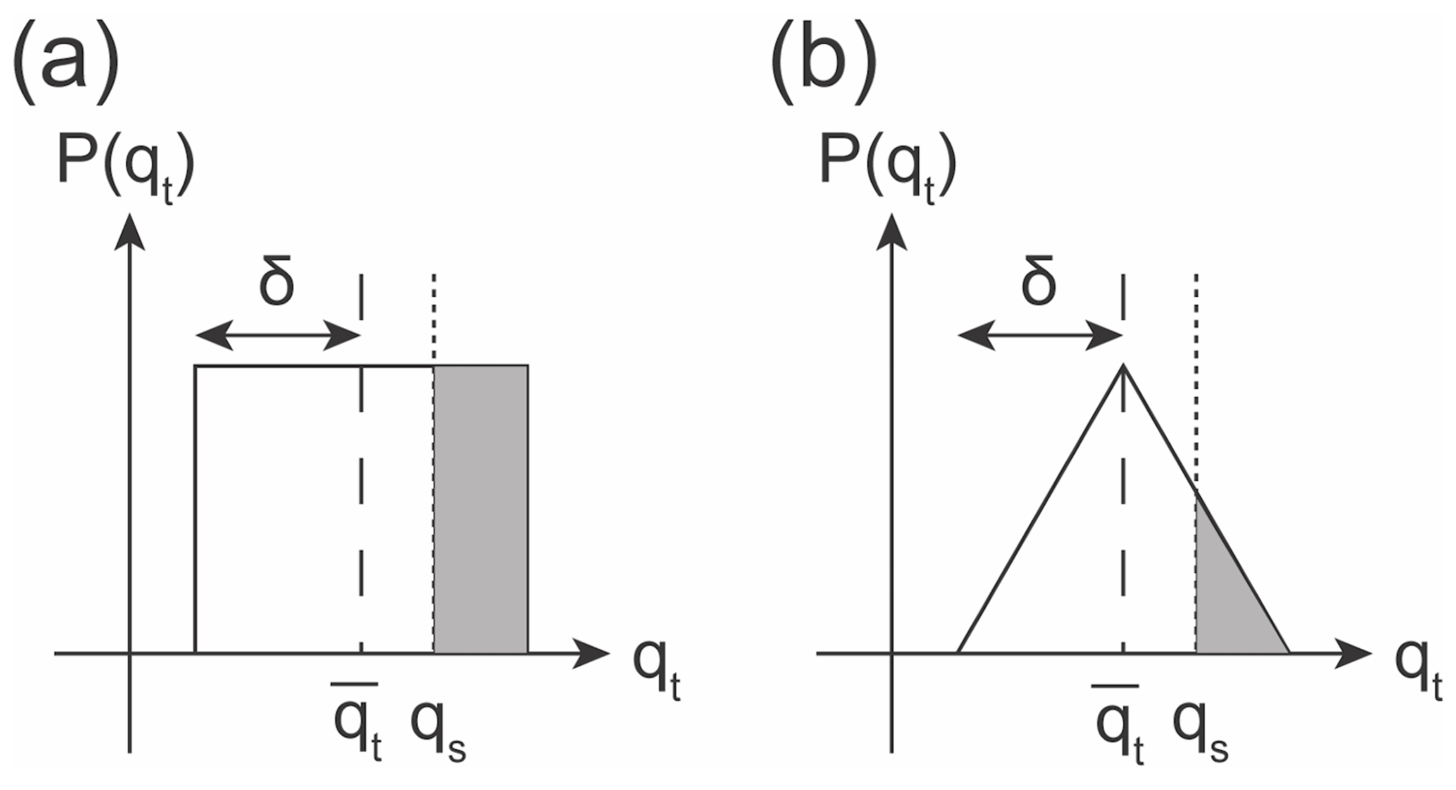
Figure 1 Illustration of subgrid PDF of total water substance q_t with (a) uniform distribution and (b) triangular distribution. The shaded part shows the saturated cloud fraction, δ represents the width of the PDF, $\stackrel{\mathrm{‾}}{q_{\mathrm{t}}}$ denotes the grid-mean value of total water substance, and q_s represents the saturation mixing ratio as the temperature is assumed to be uniform within the grid. Please note that uniform temperature assumption is used for the GTS cloud macrophysics.

2 Descriptions of scheme, model, and simulation setup

2.1 Scheme descriptions

Figure 1 illustrates the PDF-based scheme with a uniform PDF and a triangular PDF of total water substance q_t. By assuming that the clear region is free of condensates and that the cloudy region is fully saturated, the cloudy region (b) becomes the area where q_t is larger than the saturation value q_s (shaded area). The PDF-based scheme automatically retains consistency between CF and condensates because it is derived from the same PDF. Here, we used the uniform PDF to demonstrate the relationship between RH_c and the width of the PDF. Using a derivation extended from Tompkins (2005),

$$\begin{array}{}\text{(2)}& b={\displaystyle \frac{\mathrm{1}}{\mathrm{2}\mathit{\delta }}}(\stackrel{\mathrm{‾}}{q_{\mathrm{t}}}+\mathit{\delta }-q_{\mathrm{s}}).\end{array}$$

It is evident that, with the uniform PDF,

$$\begin{array}{}\text{(3)}& {\mathit{\delta }}_{\mathrm{c}}=q_{\mathrm{s}}\left(\mathrm{1}-{\mathrm{RH}}_{\mathrm{c}}\right).\end{array}$$

Therefore, ${\mathrm{RH}}_{\mathrm{c}}=\mathrm{1}-\frac{{\mathit{\delta }}_{\mathrm{c}}}{q_{\mathrm{s}}}$. Thus, if the width δ of the uniform PDF is determined, then RH_c can be determined accordingly. This relation reveals that the RH_c assumption of the RH-based scheme actually assumes the width of the uniform PDF to be δ_c from the PDF-based scheme. As noticed by Tompkins (2005), the RH_c used by Sundqvist et al. (1989) for cloud generation can be linked to the statistical cloud scheme with a uniform distribution. Building upon this finding, we eliminated the assumption of RH_c by determining the P(q_t) with information about $\stackrel{\mathrm{‾}}{q_{\mathrm{v}}}$ and $\stackrel{\mathrm{‾}}{q_{\mathrm{l}}}$ provided by the base model. Please note that uniform temperature is assumed over the grid for the GTS scheme.

With uniform PDF as denoted in Fig. 1a, the liquid cloud fraction (b_l) and grid-mean cloud liquid mixing ratio ($\stackrel{\mathrm{‾}}{q_{\mathrm{l}}}$) can be integrated as follows:

$$\begin{array}{}\text{(4)}& b_{\mathrm{l}}=\underset{q_{\mathrm{s}}}{\overset{\mathrm{\infty }}{\int }}P\left(q_{\mathrm{t}}\right)d{q}_{\mathrm{t}}={\displaystyle \frac{\mathrm{1}}{\mathrm{2}\mathit{\delta }}}\left(\stackrel{\mathrm{‾}}{q_{\mathrm{l}}}+\stackrel{\mathrm{‾}}{q_{\mathrm{v}}}+\mathit{\delta }-q_{\mathrm{s}}\right),\end{array}$$

and

$$\begin{array}{}\text{(5)}& \stackrel{\mathrm{‾}}{q_{\mathrm{l}}}=\underset{q_{\mathrm{s}}}{\overset{\mathrm{\infty }}{\int }}(q_{\mathrm{t}}-q_{\mathrm{s}})P\left(q_{\mathrm{t}}\right)d{q}_{\mathrm{t}}={\displaystyle \frac{\mathrm{1}}{\mathrm{4}\mathit{\delta }}}\left({\stackrel{\mathrm{‾}}{q}}_{\mathrm{t}}+\mathit{\delta }-q_{\mathrm{s}}\right).\end{array}$$

Given $\stackrel{\mathrm{‾}}{q_{\mathrm{l}}}$, $\stackrel{\mathrm{‾}}{q_{\mathrm{v}}}$, and q_s, the width of uniform PDF can be determined as follows:

$$\begin{array}{}\text{(6)}& \mathit{\delta }={\left(\sqrt{\stackrel{\mathrm{‾}}{q_{\mathrm{l}}}}+\sqrt{q_{\mathrm{s}}-\stackrel{\mathrm{‾}}{q_{\mathrm{v}}}}\right)}^{\mathrm{2}}.\end{array}$$

Therefore, we can calculate the liquid cloud fraction from Eq. (4).

In addition to the application of a PDF-based approach for liquid CF parameterization, the GTS scheme also uses the same concept for parameterizing the ice CF (b_i) as follows:

$$\begin{array}{}\text{(7)}& b_{\mathrm{i}}={\displaystyle \frac{\mathrm{1}}{\mathrm{2}\mathit{\delta }}}({\stackrel{\mathrm{‾}}{q}}_{\mathrm{i}}+{\stackrel{\mathrm{‾}}{q}}_{\mathrm{v}}+\mathit{\delta }-\sup \cdot q_{\mathrm{si}}),\end{array}$$

where ${\stackrel{\mathrm{‾}}{q}}_{\mathrm{i}}$, ${\stackrel{\mathrm{‾}}{q}}_{\mathrm{v}}$, and q_si denote the grid-mean cloud ice mixing ratio, water vapor mixing ratio, and saturation mixing ratio over ice, respectively. In Eq. (7), q_si is multiplied by a supersaturation factor (“sup”) to account for the situation in which rapid saturation adjustment is not reached for cloud ice. In the present version of the GTS scheme, sup is temporarily assumed to be 1.0. Sensitivity tests regarding sup will be discussed in Sect. 5.6. Values of $\stackrel{\mathrm{‾}}{q_{\mathrm{i}}}$ and $\stackrel{\mathrm{‾}}{q_{\mathrm{v}}}$ used to calculate Eq. (7) are the updated state variables before calling the cloud macrophysics process.

A more complex PDF can be used for P(q_t) instead of the uniform distribution in our derivation. For example, the Community Atmosphere Model version 5.3 (CAM5.3) macrophysics model adopts a triangular PDF instead of a uniform PDF to represent the subgrid distribution of the total water substance (Park et al., 2014). Mathematically, the triangular distribution is a more accurate approximation of the Gaussian distribution than the uniform distribution and it may also be more realistic. Therefore, we followed the same procedure to diagnose the CF by forming a triangular PDF with $\stackrel{\mathrm{‾}}{q_{\mathrm{l}}}$, $\stackrel{\mathrm{‾}}{q_{\mathrm{v}}}$, and $\stackrel{\mathrm{‾}}{q_{\mathrm{s}}}$ provided. Moreover, by using a triangular PDF, we can obtain results that are more comparable to the CAM5.3 macrophysics scheme because the same PDF was used. By considering the PDF width, the CF (b) and liquid water content ($\stackrel{\mathrm{‾}}{q_{\mathrm{l}}}$) can be written as follows:

$$\begin{array}{}\text{(8)}& b=\left\{\begin{array}{lll}\frac{\mathrm{1}}{\mathrm{2}}{\left(\mathrm{1}-s_{\mathrm{s}}\right)}^{\mathrm{2}}& \text{if}& s_{\mathrm{s}}>\mathrm{0}\\ \mathrm{1}-\frac{\mathrm{1}}{\mathrm{2}}{\left(\mathrm{1}+s_{\mathrm{s}}\right)}^{\mathrm{2}}& \text{if}& s_{\mathrm{s}}<\mathrm{0}\end{array}\right.,\end{array}$$

and

$$\begin{array}{}\text{(9)}& {\displaystyle \frac{\stackrel{\mathrm{‾}}{q_{\mathrm{l}}}}{\mathit{\delta }}}=\left\{\begin{array}{lll}\frac{\mathrm{1}}{\mathrm{6}}-\frac{s_{\mathrm{s}}^{\mathrm{2}}}{\mathrm{6}}+\frac{s_{\mathrm{s}}^{\mathrm{3}}}{\mathrm{6}}-s_{\mathrm{s}}b& \text{if}& s_{\mathrm{s}}>\mathrm{0}\\ -\frac{\mathrm{1}}{\mathrm{6}}-\frac{\mathrm{1}}{\mathrm{6}}\left(\mathrm{3}{s}_{\mathrm{s}}^{\mathrm{2}}-\mathrm{2}{s}_{\mathrm{s}}^{\mathrm{3}}\right)-s_{\mathrm{s}}b& \text{if}& s_{\mathrm{s}}<\mathrm{0}\end{array}\right.,\end{array}$$

respectively, where $s_{\mathrm{s}}=\frac{q_{\mathrm{s}}-\stackrel{\mathrm{‾}}{q_{\mathrm{t}}}}{\mathit{\delta }}$. From these two equations, we can derive the width of the triangular PDF and calculate the CF (b) based on q_s, $\stackrel{\mathrm{‾}}{q_{\mathrm{t}}}$, and $\stackrel{\mathrm{‾}}{q_{\mathrm{v}}}$ instead of RH_c. Detailed derivations of Eqs. (8) and (9) can be seen in Appendix A. Notably, the PDF width for the total water substance can only be constrained when the cloud exists. Therefore, the RH_c is still required when clouds start to form from a clear region. To simplify the cloud macrophysics parameterization, value of RH_c in the GTS scheme is assumed to be 0.8 instead of RH_c varying with height in the default Park scheme. The GTS scheme still uses the default prognostic scheme for calculating cloud condensates (Park et al., 2014), and it has effects only on the stratiform CFs. Although the GTS scheme is presumed to have good consistency between CF and condensates, the consistency check subroutines of the Park scheme are still kept in the GTS scheme to avoid “empty” and “dense” clouds due to the usage of the Park scheme for calculating cloud condensates, and the GTS schemes still need RH_c when clouds start to form.

In this study, GTS schemes utilizing two different PDF shape assumptions are evaluated: uniform (hereafter, U_pdf) and triangular (hereafter, T_pdf). These two PDF types are specifically formulated to evaluate the effects of the choice of PDF shape. A triangular PDF is the default shape used for cloud macrophysics by CAM5.3 (hereafter, the Park scheme). The T_pdf of the GTS scheme is numerically similar to that of the Park scheme except for using a variable width for the triangular PDF once clouds are formed.

2.2 Model description and simulation setup

The GTS schemes described in this study were implemented into CAM5.3 in the Community Earth System Model version 1.2.2 (CESM 1.2.2), which is developed and maintained by Department of Energy (DOE) University Corporation for Atmospheric Research/National Center for Atmospheric Research (UCAR/NCAR). Physical parameterizations of CAM5.3 include deep convection, shallow convection, macrophysics, aerosol activation, stratiform microphysics, wet deposition of aerosols, radiation, a chemistry and aerosol module, moist turbulence, dry deposition of aerosols, and dynamics. References for the individual physical parameterizations can be found in the NCAR technical notes (Neale et al., 2010). The master equations are solved on a vertical hybrid pressure–sigma coordinate system (30 vertical levels) using the finite-volume dynamical core option of CAM5.3.

We conducted both the single-column tests and stand-alone global-domain simulations with CAM5.3 physics. The single-column setup provides the benefit of understanding the responses of physical schemes under environmental forcing of different regimes of interest. Here, we adopt the case of Tropical Warm Pool – International Cloud Experiment (TWP-ICE), which was supported by the ARM program of the Department of Energy and the Bureau of Meteorology of Australia from January to February 2006 over Darwin in northern Australia. Based on the meteorological conditions, the TWP-ICE period can be divided into four shorter periods: the active monsoon period (19–25 January), the suppressed monsoon period (26 January to 2 February), the monsoon clear-sky period (3–5 February), and the monsoon break period (6–13 February; May et al., 2008; Xie et al., 2010). To take advantage of previous studies of cloud-resolving models and single-column models, we followed the setup of Franklin et al. (2012) to initiate the single-column runs starting on 19 January 2006 and running for 25 d.

Stand-alone CAM5.3 simulations of the CESM model, forced by climatological sea surface temperature for the year 2000 (i.e., CESM compset: F_2000_CAM5), are conducted to demonstrate global results. The horizontal resolution of the CESM global runs is set at 2^∘. Individual global simulations are integrated for 12 years, and the output for the last 10 years is used to calculate climatological means and annual cycles in global means. Because we made changes largely with respect to CF, we also conducted corresponding simulations using the satellite-simulator approach to provide CF for a fair comparison with satellite CF products and typical CESM model output. This was done using the Cloud Feedback Model Intercomparison Project (CFMIP) Observation Simulator Package (COSP) built into CESM 1.2.2 (Kay et al., 2012). In addition to the default monthly outputs, daily outputs of several selected variables are also written out for more in-depth analysis.

3 Observational datasets and offline calculations

3.1 Observational data

Cloud field comparisons are critical for modifications to our system with respect to cloud macrophysical schemes. Therefore, we use the products from CloudSat/Cloud-Aerosol Lidar and Infrared Pathfinder Satellite Observation (CALIPSO) to provide CF data for evaluating the modeling capabilities of the default and modified GTS cloud macrophysical schemes. This dataset (provided by the AMWG diagnostics package of NCAR) is used to compare with CF simulated by the COSP satellite simulator of CESM 1.2.2. Notably, this dataset is different from the one below which also includes cloud water content (CWC).

In addition to cloud observations, observational radiation fluxes from the Clouds and the Earth's Radiant Energy System – Energy Balanced and Filled (EBAF) product (CERES-EBAF) are also used to investigate whether simulations using our system will improve radiation calculations for both shortwave and longwave radiation flux, as well as their corresponding cloud radiative forcings. Precipitation data are compared with Global Precipitation Climatology Project data and several other climatic parameters, e.g., air temperature, RH, precipitable water, and zonal wind, are evaluated against the reanalysis data (ERA-Interim). All these observational data are also obtained from the AMWG diagnostics package provided by NCAR and their corresponding datasets can be found in the NCAR Climate Data Guide (https://climatedataguide.ucar.edu/collections/diagnostic-data-sets/ncar-doe-cesm/atmosdiagnostics, last access: 8 January 2021). The time periods used to calculate the climatological means are simply following the default setup of the AMWG diagnostics package.

We further evaluate the performance of the three macrophysics schemes by using the approach of Su et al. (2013), which compares CF and CWC sorted by large-scale dynamical and thermodynamic parameters. The CF products are based on the 2B-GEOPROF R04 dataset (Marchand et al., 2008), while the CWC data are based on the 2B-CWC-RO R04 dataset (Austin et al., 2009). The methodology from Li et al. (2012) is used to generate gridded data. Two independent approaches (i.e., FLAG and PSD methods) are used in Li et al. (2012) to distinguish ice mass associated with clouds from ice mass associated with precipitation and convection. The PSD method is used in this study (Chen et al., 2011). In total, 4 years of CloudSat/CALIPSO data, from 2007 to 2010, are used to carry out the statistical analyses. These data are used to obtain overall climatological means to compare to those obtained from model simulations instead of undergoing rigorous year-to-year comparisons between observations and simulations. Monthly data from ERA-Interim for the same 4 years are used to obtain the dynamical and thermodynamic parameters used in Su et al.'s approach. These parameters include large-scale vertical velocity at 500 mbar and RH at several vertical levels.

Figure 2 Mean cloud fraction in July (a) from the ERA-Interim reanalysis dataset and (b, c, d) diagnosed from cloud fraction schemes, with temperature, moisture, and condensates from the ERA-Interim reanalysis provided. From left to right, these schemes are the (b) U_pdf, (c) T_pdf, and (d) Park macrophysics schemes. Cloud distributions from 100 to 900 hPa are plotted from top to bottom. Also shown are values of global annual means.

3.2 Offline calculation of cloud fraction

To evaluate the impact of assumptions of CF distributions for the RH- and PDF-based schemes, we conducted offline calculations of the CF by using the reanalyzed temperature, humidity, and condensate data from ERA-Interim. As the differences in CF characteristics do not change from month to month, the results for July are shown in Fig. 2 as an example. The ERA-Interim reanalysis performed by Dee et al. (2011) using a 0.75^∘ resolution from 1979 to 2012 is used in the calculation. With this offline approach, we can observe the impacts of these macrophysics assumptions with a balanced atmospheric state provided by the reanalysis.

Using the U_pdf of GTS scheme as an example to elaborate on the details of calculation procedures, we simply obtain the cloud liquid mixing ratio ($\stackrel{\mathrm{‾}}{q_{\mathrm{l}}}$), water vapor mixing ratio ($\stackrel{\mathrm{‾}}{q_{\mathrm{v}}}$), and air temperature (to calculate $\stackrel{\mathrm{‾}}{q_{\mathrm{sl}}}$) from the ERA-Interim as input variables to calculate the liquid CF via using Eqs. (6) and (4) when $\stackrel{\mathrm{‾}}{q_{\mathrm{l}}}$ is greater than 10⁻¹⁰ (kg kg⁻¹). When $\stackrel{\mathrm{‾}}{q_{\mathrm{l}}}$ is smaller than 10⁻¹⁰ (kg kg⁻¹) and if RH>RH_c, CFs are calculated based on Eq. (3) and the liquid CF parameterization of Sundqvist et al. (1989), and if RH<RH_c, CFs are equal to zero. Ice CFs are calculated similarly to those of liquid CFs but using Eq. (7), ${\stackrel{\mathrm{‾}}{q}}_{\mathrm{i}}$, ${\stackrel{\mathrm{‾}}{q}}_{\mathrm{si}}$, and sup of 1.0. Procedures for calculating CFs diagnosed by the T_pdf of the GTS scheme are similar to those of U_pdf but using the equation set of the triangular PDF. Values of RH_c used in the U_pdf and T_pdf of GTS schemes are assumed to be 0.8 and height independent. The maximum overlapping assumption is used to calculate the horizontal overlap between the liquid CF and ice CF.

Overall, the geographical distributions from the two GTS schemes are similar to that of the ERA-Interim reanalysis shown in Fig. 2. In July, high clouds corresponding to deep convection are shown over south and east Asia where monsoons prevail. The diagnosed clouds of the GTS scheme have a maximum level of 125 hPa, which is consistent with those of the ERA-Interim reanalysis but also have a more extensive cloud coverage of up to 90 %. Below the freezing level at approximately 500 hPa, the CF diagnosed by the GTS scheme is comparable to that diagnosed by ERA-Interim reanalysis. The most substantial differences in CF between the GTS scheme and ERA-Interim are observed in the mixed-phase clouds, such as the low clouds over the Southern and Arctic oceans. Such differences suggest that more complexity in microphysics assumptions may be needed to describe the large-scale balance of mixed-phase clouds. It is interesting to note that the U_pdf simulates CFs at the lower levels in closer agreement with those of ERA-Interim and the U_pdf obtains similar magnitude of CFs to those of the T_pdf at the upper levels. The potential reason for such differences could be related to the nature of the two PDFs. The U_pdf is likely to calculate more CFs compared to T_pdf given similar RH and cloud liquid mixing ratio in the lower atmospheric levels. The diagnosed CF for the Park macrophysics scheme is also shown in the right column of Fig. 2. We found that the cloud field diagnosed by the Park macrophysics scheme was considerably different from that diagnosed by ERA-Interim reanalysis and the GTS schemes. The Park scheme diagnosed overcast high clouds of 100–125 hPa with coverage of up to 100 % over the warm pool and Intertropical Convergence Zone, but very little cloud coverage below 200 hPa, suggesting that the assumptions of the Park scheme are probably not suitable for large-scale states of the ERA-Interim reanalysis.

However, such a calculation does not account for the feedback of the clouds to the atmospheric states through condensation or evaporation and cloud radiative heating. Therefore, we further extended our single-column CAM5.3 experiments to examine the impact of the cloud PDF assumption.

4 Single-column results

This section presents the analysis of single-column simulations using the TWP-ICE field campaign. We focused on the CF fields and humidity fields to see how the RH_c assumption affects these features through humidity partitioning. Five sets of model experiments were conducted. In addition to the T_pdf and U_pdf of the GTS and Park schemes, we also include the T_pdf and U_pdf of the GTS scheme with the Slingo ice CF parameterization. These experiments can help us to interpret the impacts of RH_c on liquid and ice CFs separately.

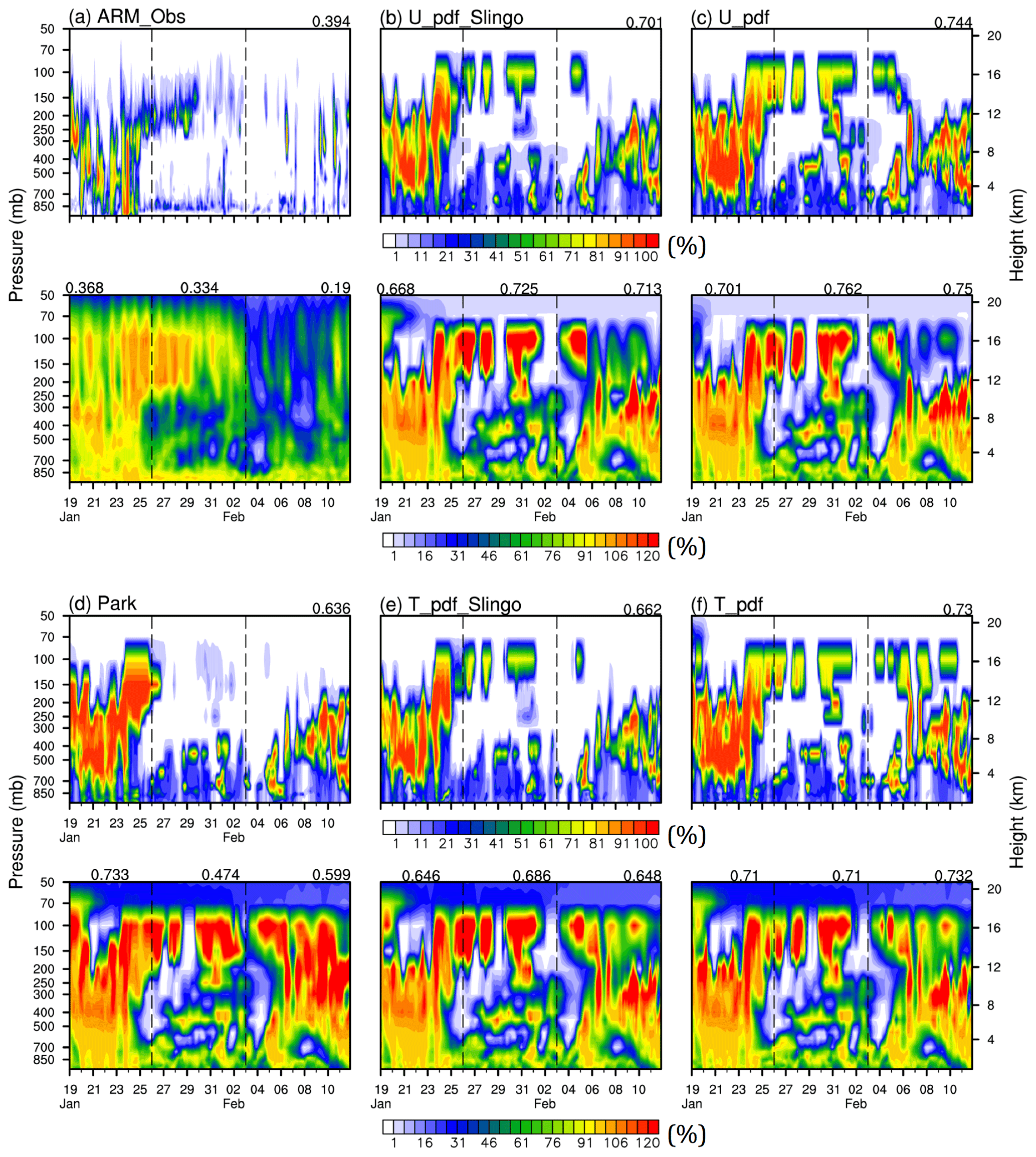
Figure 3 Pressure–time cross-sections of cloud fraction (upper panel) and relative humidity (lower panel) observed by (a) Xie et al. (2010) and simulated by SCAM with the (b) U_pdf with Slingo ice CF scheme, (c) U_pdf, (d) Park of CAM5.3, (e) T_pdf with Slingo ice CF scheme, and (f) T_pdf cloud macrophysics schemes. Values shown in the upper sections of panels (a)–(f) represent pressure–time pattern correlation coefficients between cloud fraction and relative humidity during the whole time period. Similarly, values shown in the lower sections of panels (a)–(f) represent pattern correlation coefficients between cloud fraction and relative humidity during the first, second, and third time periods as separated by the dashed lines.

Figure 3 shows the correlation between CF and RH for the three time periods during the TWP-ICE. As expected, the correlation coefficients are quite similar for the individual schemes during the active monsoon period when convective clouds dominated (R=0.73, Park, vs. 0.71, T_pdf, vs. 0.70, U_pdf). In contrast, the correlation coefficient between CF and RH differs during the suppressed monsoon period when stratiform clouds dominated (R=0.47, Park, vs. 0.71, T_pdf, vs. 0.76, U_pdf). The correlation coefficient between CF and RH is approximately 20 % higher for the stratiform-cloud-dominated period when using T_pdf or U_pdf in the GTS scheme. It is also worth mentioning that, during the monsoon break period when both convective and stratiform clouds coexist, the usage of the GTS scheme can also increase the correlation between CF and RH by 10 % compared to the default Park scheme. Notably, the higher correlation coefficient for stratiform-cloud-dominated areas only suggests that the GTS scheme can somehow better simulate the variation of CF associated with RH, for which stratiform cloud macrophysics parameterization normally takes effect in CAM5.3.

Comparisons between T_pdf with the Slingo ice CF and the Park scheme can be used to examine the role of applying a PDF-based approach in simulating the liquid CF in the GTS scheme. The use of a PDF-based approach for calculating the liquid CF can increase the correlation between CF and RH by approximately 12 % during the suppressed monsoon period (R=0.69, T_pdf with Slingo, vs. 0.47, Park). Such an outcome also suggests that implementing a PDF-based approach for liquid clouds can lead to more reasonable fluctuations between CF and RH in GCM grids.

It turns out that using the PDF-based approach for ice clouds slightly contributes to the increased correlation between CF and RH, as shown in Fig. 3 with the T_pdf scheme (R=0.69, T_pdf with Slingo, vs. 0.71, T_pdf) or U_pdf scheme (R=0.73, U_pdf with Slingo, vs. 0.76, U_pdf). Such results also suggest that extending this PDF-based approach for ice clouds can better simulate changes in the ice cloud fraction using an RH-based approach rather than an RH_c-based approach. Notably, such pair comparisons (i.e., T_pdf with Slingo ice cloud fraction scheme vs. T_pdf and vs. Park) only reveal the important features of the GTS scheme, such as how variations in liquid CF are better correlated with changes in RH of the GCM grids when compared to that of the default cloud macrophysics scheme. In fact, such high correlations between CF and RH seen in the GTS and Park schemes are not consistent with those of observations as shown in Fig. 3a, suggesting that, in nature, CF and RH are likely to be non-linear.

Admittedly, it is not easy to directly use the observational CF of the TWP-ICE field campaign to evaluate the performance of stratiform cloud macrophysics schemes in the SCAM simulations due to the coexistence of other CF types determined by the deep and shallow convective schemes as well as cloud overlapping treatments in both horizontal and vertical directions. As expected, correlation coefficients between the simulated and observed CFs are not high and their values do not differ a lot among the five cloud macrophysics schemes (Table S1 in the Supplement).

Figure 4 Scatter plots of high-level (50–300 hPa) relative humidities and cloud fractions during the suppressed monsoon period of the TWP-ICE field campaign (26 January to 3 February 2006) observed by (a) Xie et al. (2010) and simulated by SCAM with the (b) U_pdf with Slingo ice CF scheme, (c) U_pdf, (d) Park of CAM5.3, (e) T_pdf with Slingo ice CF scheme, and (f) T_pdf cloud macrophysics schemes. Two dashed blue lines are also shown in the figure to enclose the observational RH–CF distributions.

To minimize possible interference from deep and shallow convective CFs, we picked up the stratiform-cloud-dominated levels and time period to examine the CF–RH distributions. Figure 4 shows scatter plots of RH and CF between 50 and 300 hPa determined from observations (Xie et al., 2010) and simulated by models run for the suppressed monsoon period from the TWP-ICE case. It turns out that the CF–RH distributions simulated by the GTS schemes (Fig. 4c and f) are closer to those of the observational results (Fig. 4a) except under more overcast conditions (i.e., RH >70 % and RH >110 %). In contrast, the CF–RH distributions simulated by the Park scheme are much less consistent with those of observations (Fig. 4d vs. 4a). On the other hand, by excluding PDF-based treatment for the ice cloud fraction in the GTS scheme, a more obvious spread in the CF–RH distribution is produced (comparing Fig. 4b and c or 4e and f). In other words, the comparisons shown in Fig. 4 suggest that applying a PDF-based treatment for both liquid and ice CF parameterizations can simulate the CF–RH distributions in better agreement with the observational results.

Table 1 Root-mean-square errors (RMSEs) for comparisons of latitude–height cross-sections of CF among the three macrophysical schemes (Park: default scheme; T_pdf: triangular PDF in the GTS scheme; U_pdf: uniform PDF in the GTS scheme) and observational data from CloudSat/CALIPSO (Fig. 6). Comparisons are made of the means for five latitudinal ranges and three periods (JJA: June, July, August; DJF: December, January, February). The smallest RMSE value of the three schemes in each case is bold.

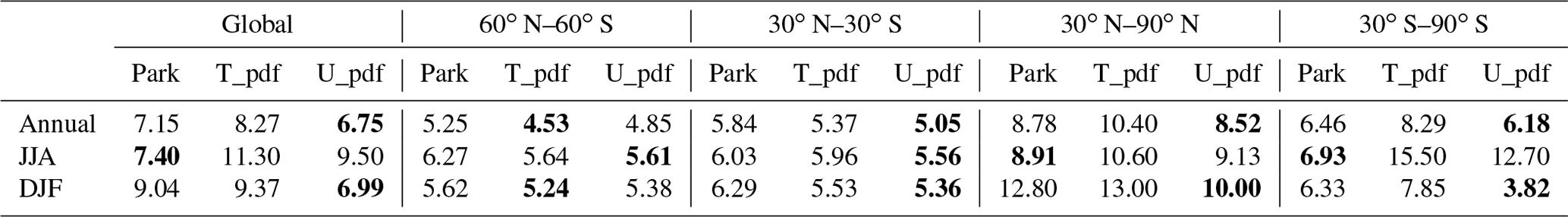
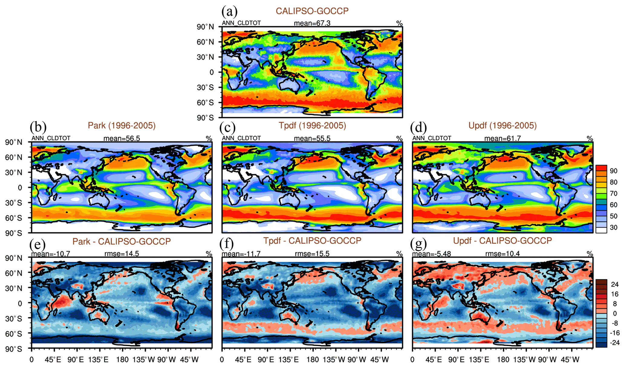
Figure 5 Total CF from (a) CALIPSO-GOCCP and simulated by the three schemes: (b) the default Park, (c) T_pdf, and (d) U_pdf, using the COSP satellite simulator of the NCAR CESM model. Differences between the simulated and observed total CFs derived from (e) the default Park, (f) T_pdf, and (g) U_pdf schemes. Also shown are values of global annual means (mean) and root mean square error (rmse) evaluated against CALIPSO-GOCCP.

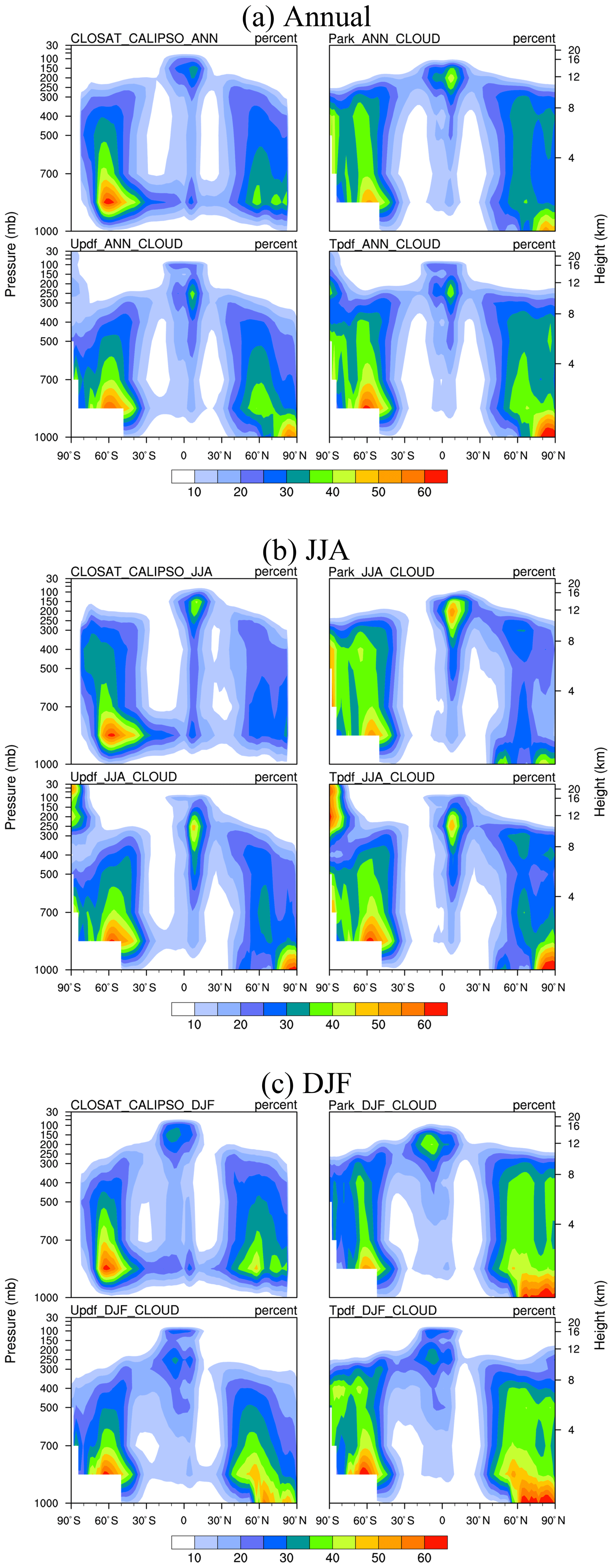
Figure 6 Latitude–height cross-sections of (a) annual, (b) June–July–August (JJA), and (c) December–January–February (DJF) mean CFs from CloudSat/CALIPSO data (upper left) and the Park (upper right), U_pdf (lower left), and T_pdf (lower right) schemes.

5 Global-domain results

5.1 Impacts on cloud fields

5.1.1 Cloud fraction

In Fig. 5, total CF simulated by the GTS schemes and the CESM default cloud macrophysics scheme, obtained from the COSP satellite simulator of the AMWG package of NCAR CESM, is compared with the total CF in CALIPSO-GOCCP. Notably, the following comparisons for the CF and associated variables are not only affected by the changes in the cloud macrophysics but also contributed by the deep and shallow convective schemes as well as cloud overlapping assumptions in the horizontal and vertical directions. Both global mean and RMSE values are improved by applying U_pdf in the GTS scheme. The CF simulation resulting from the use of U_pdf in the GTS scheme is qualitatively similar to that of CloudSat/CALIPSO, especially over the mid- and high-latitude regions and for the annual and December–January–February (DJF) simulations (Fig. 6). On the other hand, the results of the Park scheme show clouds at higher altitudes in the tropics in closer agreement with CloudSat/CALIPSO than those of U_pdf or T_pdf. Cross-section comparison of the zonal height shows that the CF simulation using U_pdf and T_pdf in the GTS scheme agrees better with that of CloudSat/CALIPSO than that produced by Park under most scenarios (globally, within 60^∘ N–60^∘ S, and within 30^∘ N–30^∘ S), especially for the annual and DJF simulations (Table 1). In contrast, some scenarios show lower RMSEs when the Park scheme is used, e.g., for the June–July–August (JJA) season globally, within 30–90^∘ N, and within 30–90^∘ S. Interestingly, when high latitudes are included (i.e., 30–90^∘ N and 30–90^∘ S), U_pdf still results in the smallest RMSE values, except for during the JJA season. It is evident that some CFs are existing at the upper level in the Antarctic in JJA when U_pdf or T_pdf of GTS is used. However, such high CFs are not seen in CloudSat/CALIPSO observations, suggesting that the usage of GTS schemes could cause significant biases in CFs under such environmental conditions. This is of course highly related to the ice CF schemes of GTS. More observation-constrained adjustments or tuning of the ice CF schemes of GTS are needed to reduce the biases in CFs in similar atmospheric environments like the upper level of the Antarctic winter. Potential tuning parameters of ice CF scheme of GTS are sup and RH_c which are discussed in Sect. 5.6.3.

Table 2 RMSEs for comparisons between CF at nine pressure levels, as simulated by the three macrophysical schemes (Park, T_pdf, U_pdf) and observational data from CloudSat/CALIPSO (Fig. 7). The comparisons are made for three periods (JJA: June, July, August; DJF: December, January, February). The smallest RMSE value of the three schemes in each case is bold.

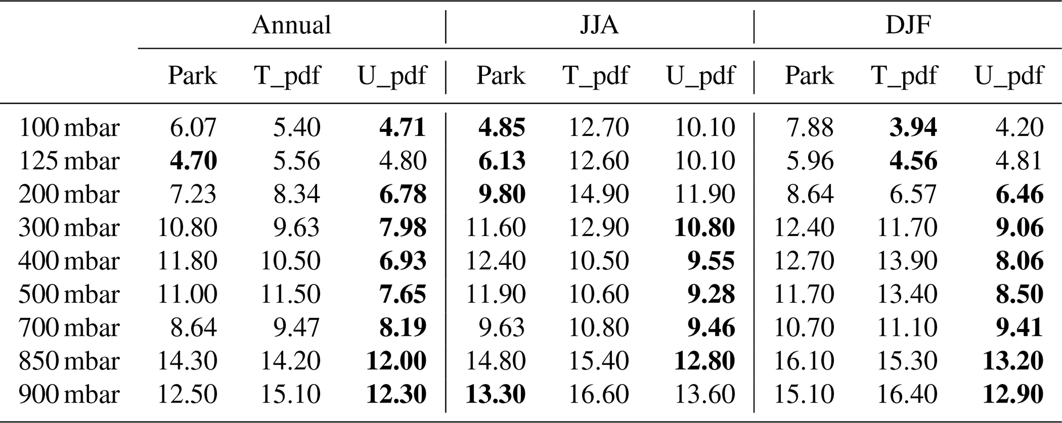
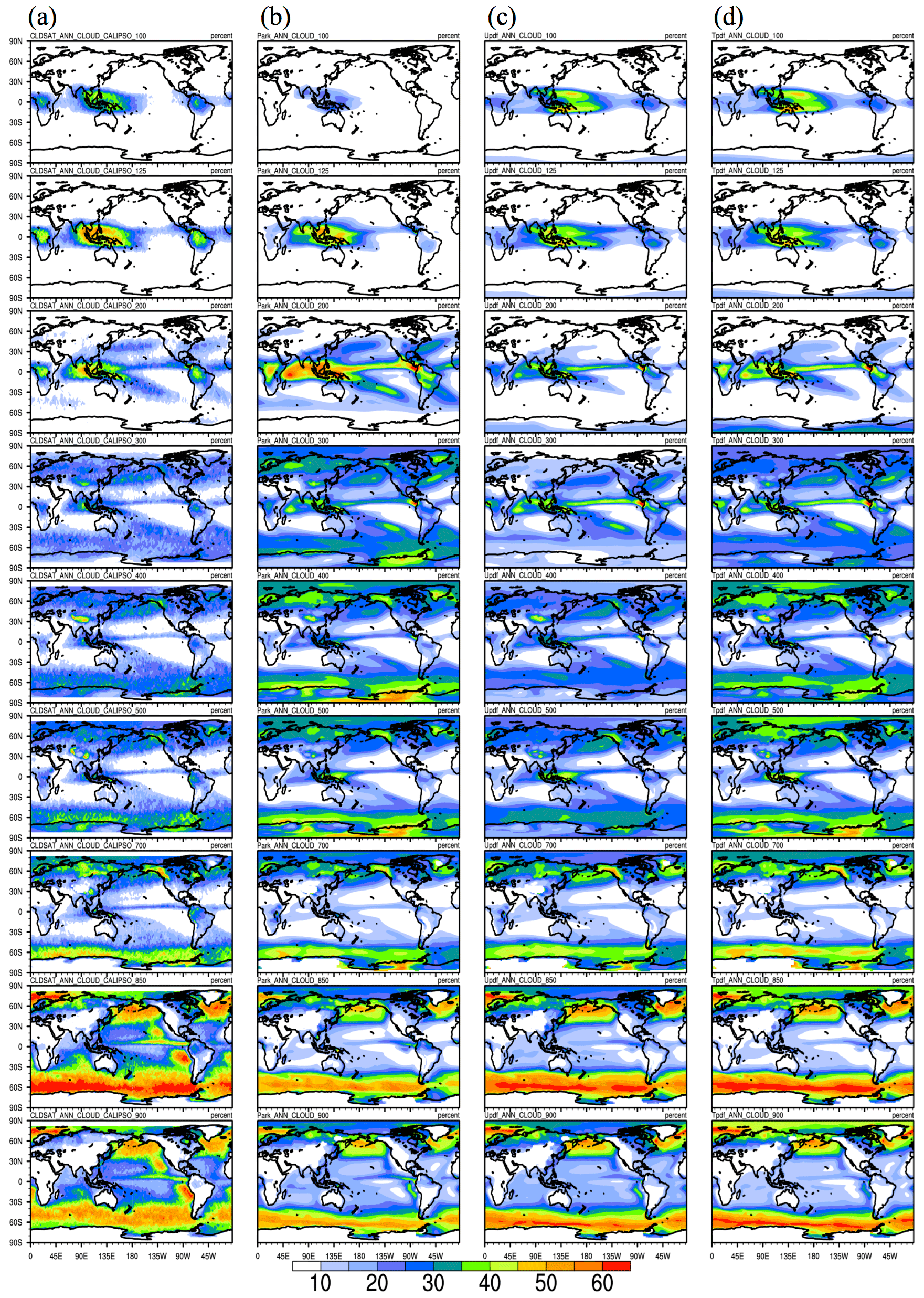
Figure 7 CFs at nine pressure levels (one pressure level per row; top to bottom: 100, 125, 200, 300, 400, 500, 700, 850, and 900 mbar) from (a) CloudSat/CALIPSO observational data and simulated by (b) the default Park, (c) U_pdf, and (d) T_pdf schemes.

We also compared the annual latitude–longitude distributions of CF at different specific pressure levels (Fig. 7). The use of U_pdf resulted in a CF simulation relatively similar to that of CloudSat/CALIPSO for mid-level clouds, i.e., 300–700 mbar, particularly for the mid- and high latitudes. However, none of the CF parameterizations are able to simulate stratocumulus clouds effectively, as revealed at the 850 and 900 mbar levels. For high clouds, the GTS and Park schemes exhibit observable differences regarding the maximum CF level. Table 2 summarizes the RMSE values for the latitude–longitude distribution of CFs at nine specific levels for the three schemes and CloudSat/CALIPSO for the annual, JJA, and DJF means. For the annual mean, U_pdf results in the smallest RMSE at all levels except at 125 mbar, for which the Park scheme yields the smallest RMSE (Table 2). For JJA, the Park scheme is closer to the observations aloft (100–200 mbar) and nearest the surface (900 mbar). For DJF, U_pdf again performs best at most levels except 100 and 125 mbar, for which T_pdf is slightly better, while for JJA, U_pdf is only best for most of the levels below 300 mbar. Overall, U_pdf in the GTS scheme results in better latitude–longitude CF distributions for 300–900 mbar for the annual, DJF, and JJA means, suggesting improvements in CF simulation for middle and low clouds.

When annual, DJF, and JJA mean vertical CF profiles are averaged over the entire globe and between 30^∘ N and 30^∘ S, U_pdf in the GTS scheme can produce a global simulation close to that of CloudSat/CALIPSO for 200–850 mbar (Fig. S1 in the Supplement). In contrast, there is a large discrepancy between the simulated and observed CFs over the tropics. Although the GTS schemes can simulate CF profiles above 100 mbar, the height of the maximum CF is lower than that of CloudSat/CALIPSO. In contrast, the height of the maximum CF simulated by the Park scheme is similar to that of CloudSat/CALIPSO but overestimated in CF. As before, when compared with CloudSat/CALIPSO, U_pdf in the GTS scheme results in the smallest RMSE and the largest correlation coefficient of the three schemes, whether or not the lower levels are included except in JJA at 125 mbar, for which Park yields the smallest RMSE (Table S2). The reason for excluding the lower levels from the statistical results is that there may be a bias for low clouds retrieved by CloudSat due to radar-signal blocking by deep convective clouds.

The different degrees of changes for the global and tropical CFs can be attributed to the relative roles of cumulus parameterizations (both deep and shallow) and stratus cloud macrophysics and/or microphysics for the different latitudinal regions. It is expected that the GTS scheme can alter CF simulations in the mid- and high-latitude areas more than in the tropics because more stratiform clouds occur in those areas. It is also interesting to note that, although it is known that more convective clouds exist in the tropics (i.e., the cumulus parameterization contributes more to the grid CF), the GTS scheme can also affect the CF simulation over the tropics to some extent.

Table 3 RMSE and R values for comparisons between CF and CWC simulated by the three macrophysical schemes (Park, T_pdf, and U_pdf) and plotted against vertical velocity at 500 mbar (ω500) or averaged RH for 300–1000 mbar (RH300–1000, obtained from the ERA-Interim reanalysis) and observational data from CloudSat/CALIPSO (Figs. 9 and 10). The comparisons are made for three latitudinal ranges. The smallest RMSE or largest R value of the three schemes in each case is bold.

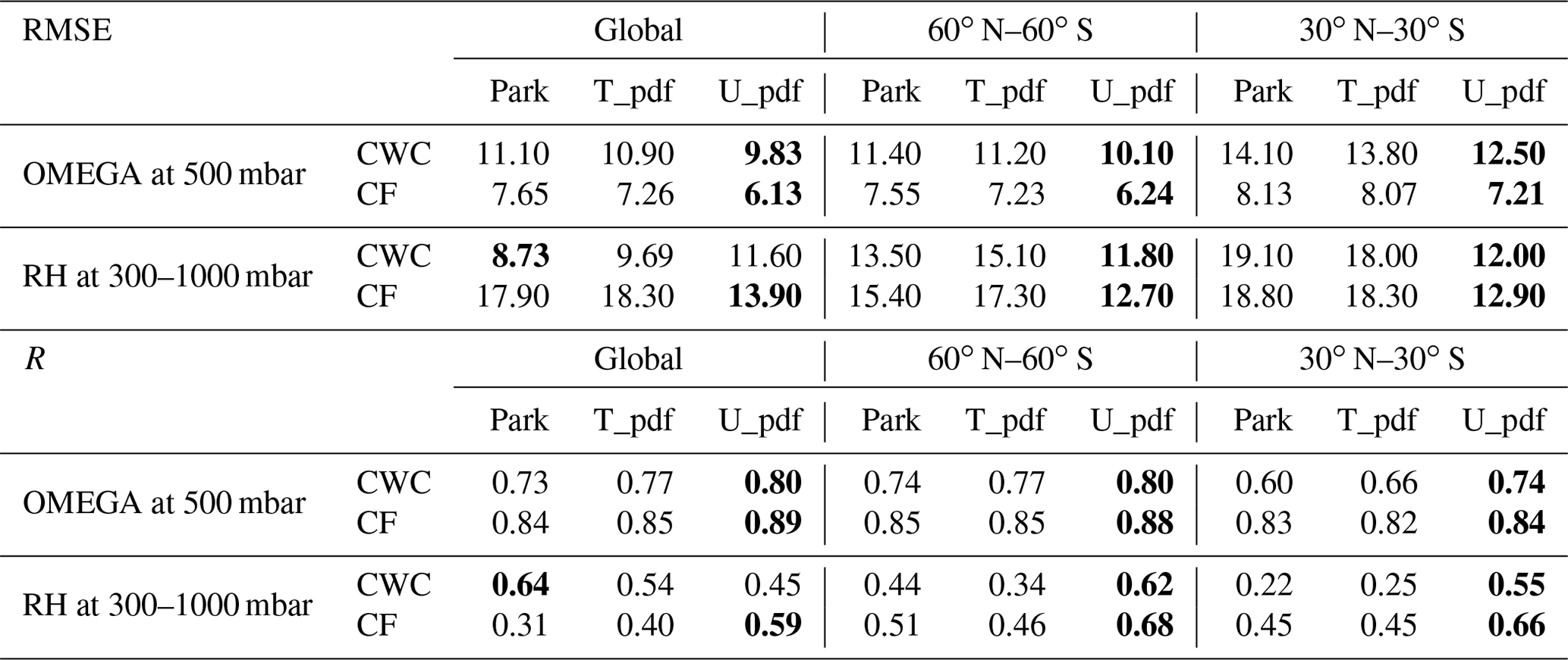
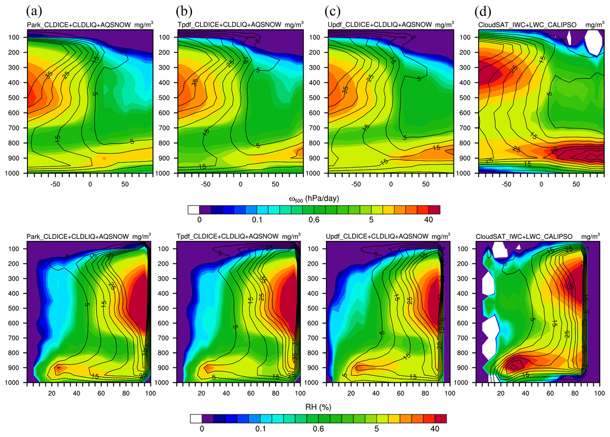
Figure 8 Vertical distribution of CF (contour lines) and CWC (colors) as functions of two large-scale parameters: vertical velocity at 500 mbar (ω500, upper four panels) and relative humidity averaged between 300 and 1000 mbar (RH300–1000, lower four panels) for the latitudinal range 30^∘ N–30^∘ S. Columns present simulations by the (a) Park, (b) T_pdf, and (c) U_pdf schemes, and (d) observational data from CloudSat/CALIPSO.

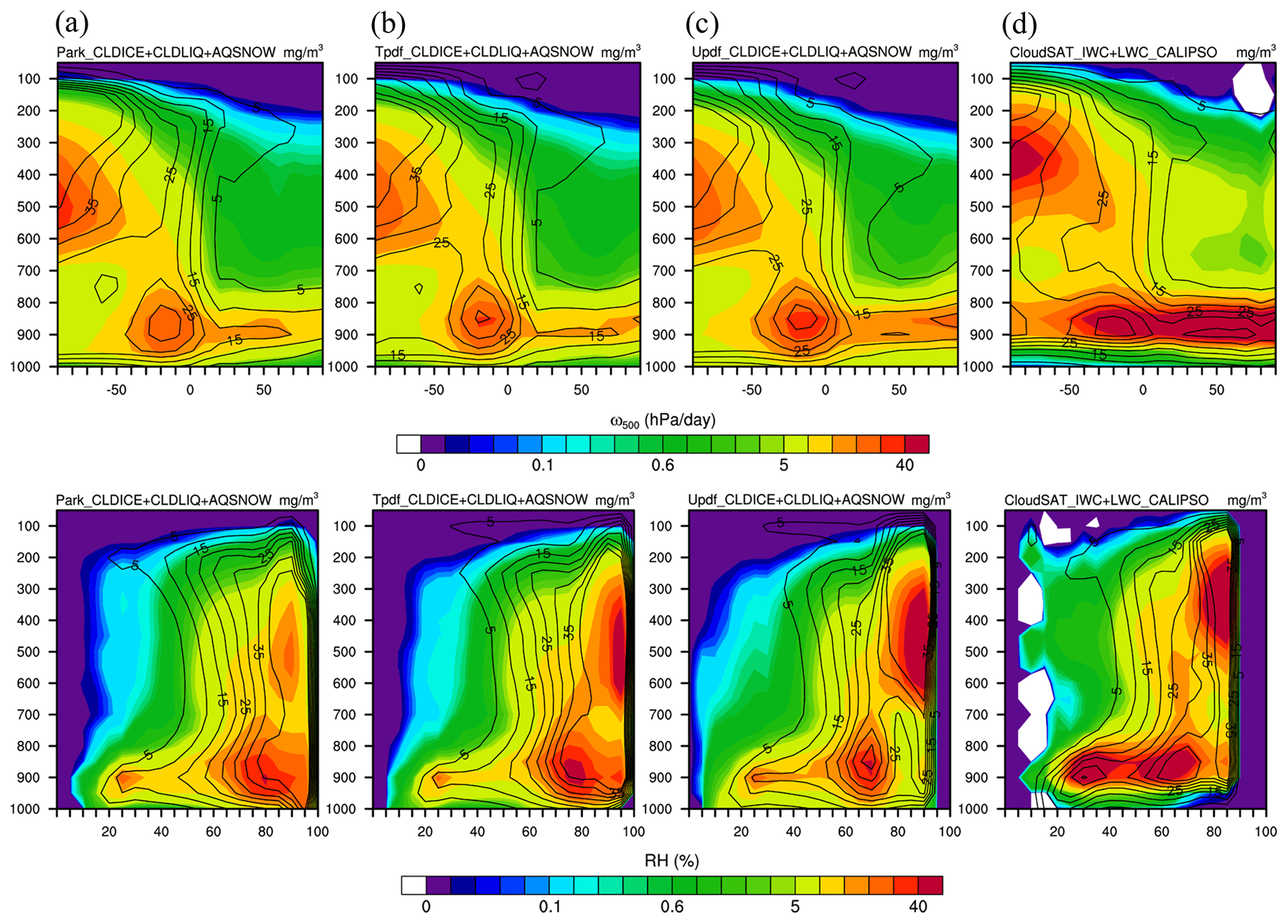
Figure 9 Vertical distribution of CF (contour lines) and CWC (colors) as functions of two large-scale parameters: ω500 (upper four panels) and RH300–1000 (lower four panels) for the latitudinal range 60^∘ N–60^∘ S. Columns present simulations by the (a) Park, (b) T_pdf, and (c) U_pdf, and (d) observational data from CloudSat/CALIPSO.

5.1.2 Cloud fraction and cloud water content

In Figs. 8 and 9, the distributions of CWC and CF as functions of large-scale vertical velocity at 500 mbar (ω500) or mean RH averaged between 300 and 1000 mbar (RH300–1000) are evaluated against CloudSat/CALIPSO observations for 30^∘ N–30^∘ S and 60^∘ N–60^∘ S. Figures 8 and 9 show that the model simulations are all qualitatively more similar to each other than to the observations. Further statistical comparisons are shown in Table 3. It is encouraging to note that, in addition to the slight improvements in CF for both of these latitudinal ranges, the use of U_pdf in the GTS scheme results in a CWC simulation that is more consistent with CloudSat/CALIPSO, whether it is plotted against ω500 or RH300–1000. The RMSE and correlation coefficient (R) values in Table 3 confirm this. For global simulations, using U_pdf also results in better agreement with CloudSat/CALIPSO for both CF and CWC when they are plotted against ω500, although for CWC plotted against RH300–1000, the Park scheme yields the smallest RMSE (Table 3). Overall, these comparisons yield results that are consistent with the general characteristics of most CMIP5 models, as found by Su et al. (2013). GCMs in general simulate the distribution of cloud fields better with respect to a dynamical parameter as opposed to a thermodynamic parameter.

It is also worth noting that the use of U_pdf yields a 20 %–30 % improvement in R when plotted against RH300–1000 for the two latitudinal ranges, 30^∘ N–30^∘ S and 60^∘ N–60^∘ S. The observable improvement in a thermodynamic parameter is an indication of the uniqueness of this GTS scheme, in that it is capable of simulating the variation in cloud fields relative to that in RH fields. There are also slight improvements in cloud fields with respect to large-scale dynamical parameters. On the other hand, the Park scheme results in an approximately 20 % improvement in R when plotted against RH300–1000 for the global domain, suggesting that the default Park scheme still simulates cloud fields better over the high latitudinal regions. It is thus worth addressing the likelihood that the different CF and CWC results for the different latitudinal ranges simulated using the GTS scheme induce cloud–radiation interaction distinct from that simulated in the Park scheme. Such changes in cloud–radiation interaction would modify not only the thermodynamic fields but also the dynamic fields in the GCMs. These changes are in turn likely to affect the climate mean state and variability. We assess and compare these potential effects in the following subsection.

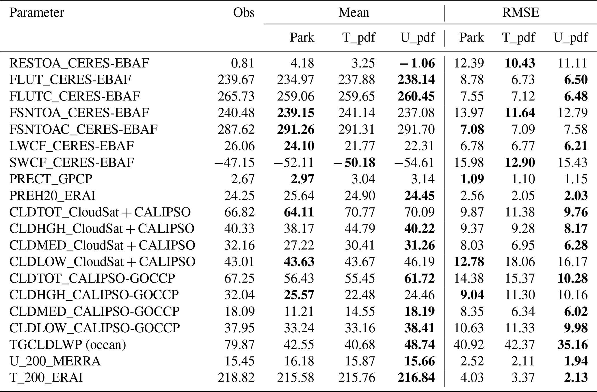
Table 4 Global annual means (mean) and RMSE values for comparisons with the observed values (obs) for a selection of climatic parameters simulated by the three cloud macrophysical schemes (Park, T_pdf, and U_pdf). The smallest RMSE value or closest global mean of the three schemes in each case is bold.

5.2 Effects on annual mean climatology

GTS schemes tend to produce smaller RMSE values for most of the global mean values of the radiation flux, cloud radiative forcing, and CF parameters shown in Table 4, suggesting that the GTS scheme is capable of simulating the variability of these variables. Furthermore, the assumed U_pdf shape appears to perform better for outgoing longwave radiation flux, longwave cloud forcing (LWCF), and CF at various levels, whereas the T_pdf assumption is better for simulating net and shortwave radiation flux at the top of the atmosphere as well as shortwave cloud forcing (SWCF) (Table 4). On the other hand, the Park scheme is better for simulating clear-sky net shortwave radiation flux and precipitation. Smaller RMSE values can also be seen for parameters such as total precipitable water, total-column cloud liquid water, zonal wind at 200 mbar (hereafter, U_200), and air temperature at 200 mbar (hereafter, T_200) when U_pdf of GTS is used. For global annual means, U_pdf simulates net radiation flux at the top of the atmosphere, all- and clear-sky outgoing longwave radiation flux, and precipitable water as well as U_200 and T_200 in closer agreement with observations. In contrast, the Park scheme is better for simulating global mean variables such as net shortwave radiation flux at the top of the atmosphere, longwave cloud forcing, and precipitation. T_pdf simulates SWCF closest to the observational mean.

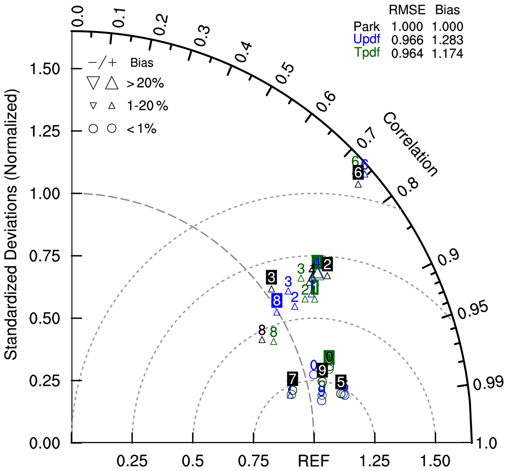
Figure 10 Space–time Taylor diagram for the 10 climatic parameters simulated by the three macrophysical schemes (Park: black symbols; U_pdf: green; T_pdf: blue) and comparisons of these with the corresponding observational data provided by the atmospheric diagnostic package from the NCAR CESM group. The 10 climatic parameters are marked from 0 to 9, where 0 denotes sea level pressure; 1 is SW cloud forcing, 2 is LW cloud forcing, 3 is land rainfall, 4 is ocean rainfall, 5 is land 2 m temperature, 6 is Pacific surface stress, 7 is zonal wind at 300 mbar, 8 is relative humidity, and 9 is temperature.

Overall, the averaged RMSE values of the 10 parameters are 0.97 and 0.96 for U_pdf and T_pdf, respectively, in the GTS schemes (Fig. 10), suggesting that using the GTS schemes would result in global simulation performance more or less similar to that of the Park scheme. It is also worth noting that the biases in RH are smallest when U_pdf in the GTS scheme is used (Table S3 in the Supplement). In contrast, T_pdf results in the smallest biases for SWCF, sea level pressure, and ocean rainfall within 30^∘ N–30^∘ S. On the other hand, the Park scheme produces the smallest biases regarding mean fields such as LWCF, land rainfall within 30^∘ N–30^∘ S, Pacific surface stress within 5^∘ N–5^∘ S, zonal wind at 300 mbar, and temperature.

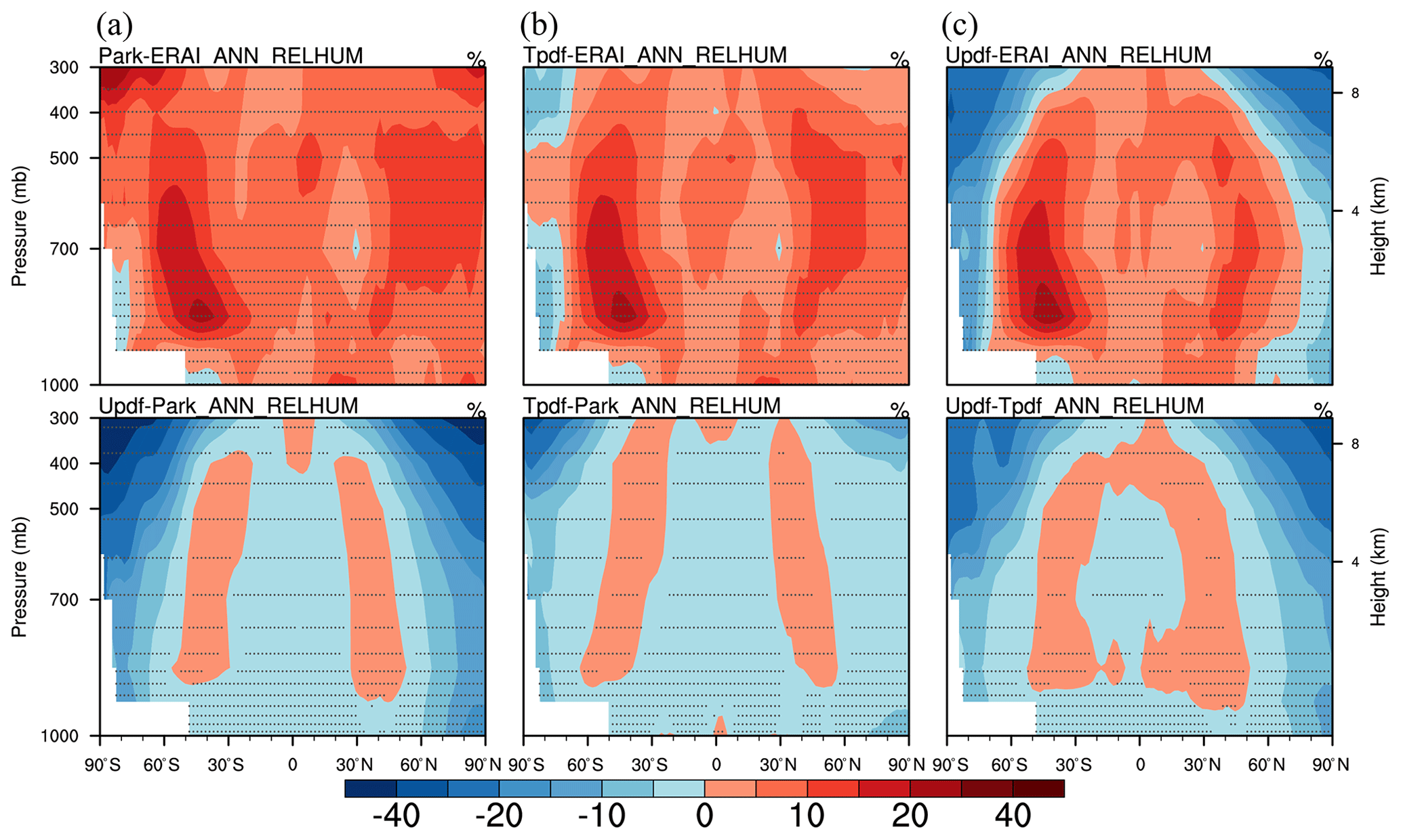
Figure 11 Upper row: latitude–pressure cross-sections of differences in relative humidity (RH) between the simulations and ERA-Interim from (a) Park, (b) T_pdf, and (c) U_pdf schemes. Lower row: differences in RH in pair-wise comparisons of the three cloud macrophysical schemes.

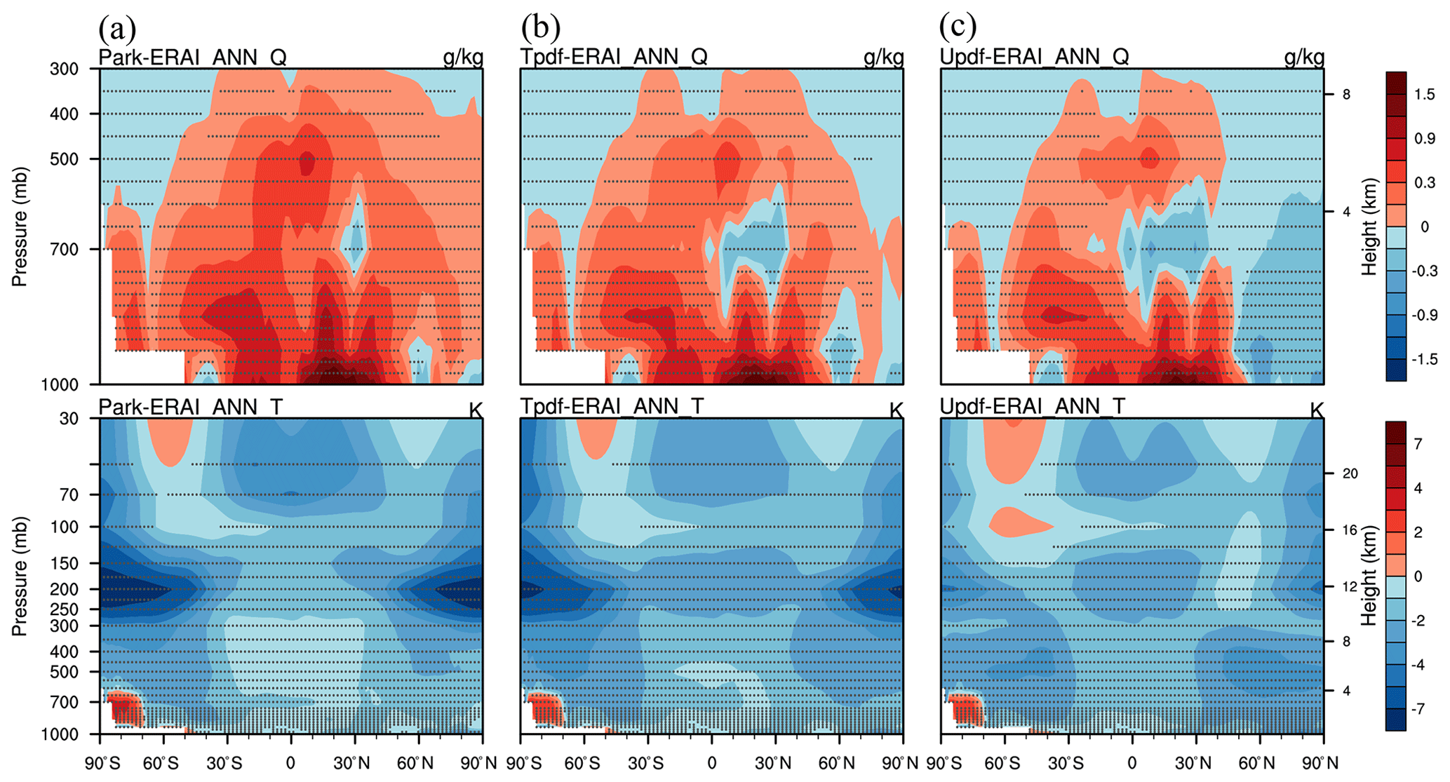
Figure 12 Differences in specific humidity (upper row) and air temperature (lower row) between the simulations and ERA-Interim from the (a) Park, (b) T_pdf, and (c) U_pdf schemes.

Comparisons of latitude–height cross-sections of RH and ERA-Interim show that the GTS schemes tend to simulate RH values smaller than the default scheme does, especially for high-latitude regions (>60^∘ N and 60^∘ S), as shown in Fig. 11. In general, in terms of RH, using T_pdf in the GTS scheme results in better agreement with ERA-Interim (Table S4). Figure 12 shows that the Park and T_pdf schemes are wetter than ERA-Interim almost everywhere and that the uniform scheme is sometimes drier. Table S5a further suggests that specific humidity simulated by the GTS schemes is slightly more consistent with ERA-Interim than the Park scheme. Comparisons of air temperature show that the three schemes tend to have cold biases almost everywhere. However, it is interesting to note that the cold biases are reduced to some extent when using the GTS schemes compared to the default scheme, as is evident in the smaller values of RMSE shown in Table S5b. These effects on moisture and temperature are likely to result in changes in the annual cycle and seasonality of climatic parameters. Such observable changes in RH, clouds (both CF and CWC), and cloud forcing suggest that the GTS scheme will simulate cloud macrophysics processes in GCMs quite differently from the Park scheme, due to the use of a variable-width PDF that is determined based on grid-mean information.

Figure 13 Upper row: differences in annual cycles of zonal mean total precipitable water between the three macrophysical schemes and the ERA-Interim data from the (a) Park, (b) T_pdf, and (c) U_pdf schemes. Lower row: differences in annual cycles of total precipitable water in pair-wise comparisons of the three cloud macrophysical schemes.

5.3 Changes in the annual cycle of climatic variables

Figure 13 shows the annual cycle of precipitable water simulated by the three schemes. The magnitude of precipitable water simulated by the GTS schemes is closer to the ERA-Interim data than the Park simulation is (Table S6). Interestingly, U_pdf results in slightly better agreement with ERA-Interim than T_pdf for the region 60^∘ N–60^∘ S. This implies that the GTS scheme would alter the moisture field for both RH and precipitable water in GCMs. These results are relatively more realistic with respect to both the moisture field and CF and CWC (Figs. 8 and 9), and are likely to yield a more reasonable cloud–radiation interaction in the GCMs. It is therefore also worth examining any differences in dynamic fields, for example, in the annual U_200 cycle, between the three schemes and the ERA-Interim data (Fig. 14). Like the annual cycle of precipitable water, U_200 simulated by the GTS schemes is closer to that of ERA-Interim than that simulated by the Park scheme (Table S6). Furthermore, the U_pdf assumption results in a better annual U_200 cycle than the T_pdf assumption, especially for 60^∘ N–60^∘ S. This further supports the argument that this GTS scheme can effectively modulate global simulations, with respect to both thermodynamic and dynamical climatic variables.

Figure 14 Upper row: differences in annual cycles of zonal wind at 200 mbar between the three macrophysical schemes and the ERA-Interim data from the (a) Park, (b) T_pdf, and (c) U_pdf schemes. Lower row: differences in annual cycles of zonal wind at 200 mbar in pair-wise comparisons of the three cloud macrophysical schemes.

Figure 15 Global annual cycles of (a) total precipitable water, (b) shortwave cloud forcing, (c) net longwave flux at the top of the model, (d) zonal wind at 200 mbar, (e) longwave cloud forcing, and (f) air temperature at 200 mbar. Colored lines represent observational data (blue) and simulations by the Park (red), U_pdf (purple), and T_pdf (green) schemes.

Figure 15 displays the global mean annual cycles of several parameters simulated by the three schemes and the corresponding parameters from observational data. The GTS scheme simulations of total precipitable water (TMQ) are close to that of ERA-Interim; indeed, U_pdf almost exactly reproduces the ERA-Interim TMQ. However, we must admit that such good agreement of the global mean is partly due to offsetting wet and dry differences from ERA-Interim. The GTS schemes also produce a more reasonable global mean annual cycle for outgoing longwave radiation (FLUT). It is probably due to the reduced CF simulated by the GTS scheme compared to the Park scheme even though the cloud top heights simulated by GTS are lower than observations in the tropics. Interestingly, for SWCF, T_pdf yields a simulation closer to the observations than the other two schemes, which is consistent with the features of the global annual mean of SWCF shown in Fig. 10 and Table S3. However, for LWCF, the annual cycle simulated by Park is closest to the observations. The U_pdf of the GTS scheme also results in improvements in U_200 and T_200 (Fig. 15). The RMSEs for all of these comparisons confirm these results (Table S7).

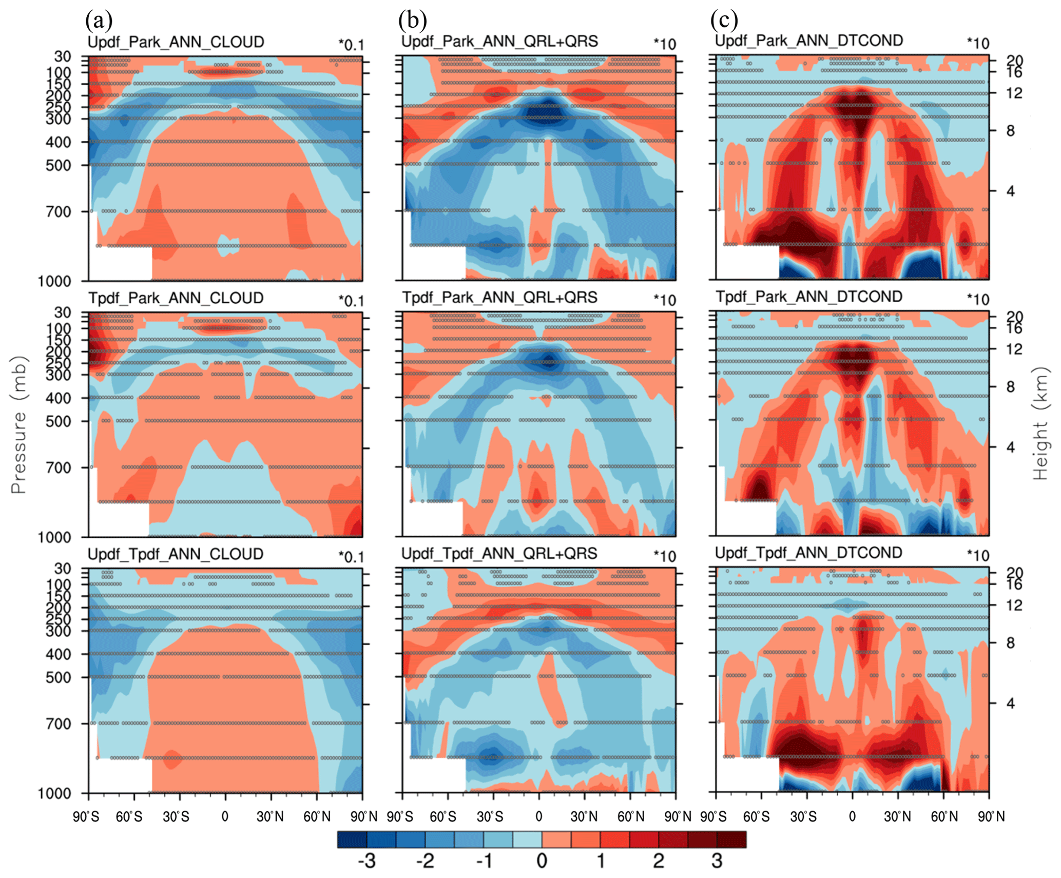
Figure 16 Differences in (a) CF (unit: %), (b) sum of longwave and shortwave heating rates (QRL + QRS, unit: K d⁻¹), and (c) temperature tendencies due to all moist processes in the NCAR CESM model (DTCOND, unit: K d⁻¹) in pair-wise comparisons of the three cloud macrophysical schemes. Upper row: U_pdf and Park; middle row: T_pdf and Park; lower row: U_pdf and T_pdf. A statistically significant difference with a confidence level of 95 % is represented in the panels by an open circle using Student's t test.

5.4 Changes in cloud–radiation interaction

As mentioned in Sect. 5.1, usage of the GTS cloud macrophysics schemes would affect the cloud fields, i.e., CF and CWC. This, in turn, is likely to affect global simulations with respect to both mean climatology and the annual cycles of many climatic parameters (as discussed in Sect. 5.2 and 5.3) through cloud–radiation interaction. Figure 16 compares CF, radiation heating rate (i.e., longwave heating rate plus shortwave heating rate, hereafter QRL + QRS), and temperature tendencies due to moist processes (hereafter, DTCOND) for each pair-wise combination of the three schemes. Qualitatively consistent changes in CF are apparent for the GTS schemes, e.g., an increase in the highest clouds over the tropics and a decrease below them, a decrease in 150–400 mbar clouds over the midlatitudes, a decrease in 300–700 mbar clouds over the high latitudes, an increase in 300–700 mbar clouds over the tropics to midlatitudes, and an increase in low clouds over the high-latitude regions. The GTS schemes also yield a significant increase in CF at atmospheric levels higher than 300 mbar over the high-latitude regions (Fig. 16). These changes affect the radiation calculations to some extent. In addition, CWC is also affected by the GTS schemes (Figs. 8 and 9). The combined effects of the changes in CF and CWC are likely to result in changes in cloud–radiation interaction. In addition, although there are significant changes in CF at high atmospheric levels in the high-latitude regions, the combined effect of CF and CWC on QRL + QRS is quite small, due to the low CWC values over this region. The changes in moisture processes, i.e., DTCOND (Fig. 16), also suggest that the combined effects of the changes in the thermodynamic and dynamical fields occur as a result of changes in cloud–radiation interaction within the GCMs from GTS schemes.

The bottom row in Fig. 16 shows the differences in CF, QRL + QRS, and DTCOND between the two GTS schemes. Relative to T_pdf, U_pdf simulates a greater CF for 300–1000 mbar clouds within 60^∘ N–60^∘ S but a smaller CF for all three cloud levels for the high-latitude regions. Furthermore, the CWC vertical cross-section also differs for the two GTS schemes (data not shown for limitations of space). Combining the changes in CF and CWC, the corresponding changes in QRL + QRS and DTCOND, particularly the increase of low clouds over the midlatitude region, are clear with an obvious decrease of high clouds over the tropical to midlatitude region. It is also evident that DTCOND simulated by the U_pdf is stronger than that simulated by the T_pdf below 700 hPa. Such enhanced condensation heating is probably contributed by the enhanced shallow convection as a result of changes in cloud–radiation interaction. However, more process-oriented diagnostics are needed to understand the complicated interaction of the moist processes.

Observable changes in large-scale circulations are likely, given the various changes in QRL + QRS and DTCOND resulting from applying different cloud macrophysics. Accordingly, both the mean and variability of the climate simulated by the GCMs differ among the three schemes, as shown in the previous subsections. These results emphasize the importance of improving cloud-related parameterization to provide better simulations of the cloud–radiation interaction within GCMs. Furthermore, as previously shown, the cloud–radiation interaction is highly sensitive to the assumptions of the CF parameterization used in the macrophysical scheme in the GCMs, even if there is only a small change in the CF parameterization. The uniqueness of the GTS scheme is in its application of a variable PDF width to calculate CF in the default PDF-based CF scheme of the CESM model. Further systematic experiments are necessary to improve our understanding of the sensitivity of the GTS scheme, and some are presented in Sect. 5.6.

Figure 17 Differences in (a) total cloud fraction, (b) shortwave cloud radiative forcing (W m⁻²), (c) longwave cloud radiative forcing (W m⁻²), and cloud fraction of (d) high clouds, (e) middle clouds, and (f) low clouds between the T_pdf and default Park schemes. Panels (g–i) are as for (d–f) but for total cloud water content at the three cloud levels. Panels (j–l) are as for (g–i) except for averaged RH at the three cloud levels.

5.5 Consistent changes in cloud radiative forcing, cloud fraction, and cloud condensates

Observable changes in clouds and radiation fluxes after adopting the GTS scheme were clearly shown in the previous subsections. It is thus worth examining features in cloud radiative forcings caused by the GTS scheme that produce such changes, as compared to those of the default Park scheme. Figure 18 shows the difference in total cloud fraction, SWCF, LWCF, CF, and averaged cloud water content, as well as the averaged RH at the three levels, i.e., 100–400, 400–700, and 700–1000 mbar, derived from the T_pdf of GTS with the Park results subtracted. One can readily observe that changes in SWCF (Fig. 17b) are quite consistent with those for total CF, showing a decrease in the total CF over the area within 30^∘ N and 30^∘ S with an increase everywhere else (Fig. 17a). Such prominent changes in latitudinal distribution of SWCF can be further related to the changes in the low (Fig. 17e) and middle (Fig. 17f) CFs particularly associated with low clouds.

On the other hand, changes in the high CF (Fig. 17d) are also quite consistent with those in LWCF (Fig. 17c), showing an overall decrease of high clouds especially over the tropical convection areas. As expected, changes in cloud water condensates (Fig. 17g–i) are closely related to changes in the CF at the three levels except for the middle clouds. Therefore, according to the evidence shown in Fig. 17a–i, it is clear that use of the GTS scheme would cause significant changes in the spatial distribution of low, middle, and high clouds (both in CF and cloud water condensates) that would result in corresponding changes in cloud radiative forcings (both for SWCF and LWCF).

Surprisingly, changes in RH at the three levels (Fig. 17j–l) are relatively less consistent with changes in the CF and condensates, especially for middle and low clouds over the mid- and high-latitude areas. Such results also indicate that there are complicated factors accounting for changes in RH in the GCMs. We suggest that, in addition to the active roles of the GTS scheme in redistributing/modulating moisture between clouds (i.e., cloud liquid or ice) and environment (water vapor) in GCM grids, thermodynamic and dynamical feedback resulting from cloud–radiation interaction also contributes to RH changes. At the present stage, we cannot quantify these individual contributions. More in-depth analysis is needed to unveil the detailed mechanisms of why GTS schemes tend to produce less low clouds over the tropics while more low clouds over the mid- and high latitudes compared to the default Park scheme, as well as observable changes regarding middle and high clouds.

5.6 Uncertainty in GTS cloud fraction parameterization

5.6.1 Assumption of PDF shape in the GTS scheme

In general, the simulations of CF, RH, and other parameters (e.g., global annual mean and/or annual cycle) using the T_pdf scheme that have been discussed and illustrated thus far have distribution features qualitatively and values quantitatively between those of the Park and U_pdf schemes. In other words, the characteristics of the T_pdf simulations are a combination of those from both the default Park scheme and the U_pdf scheme. This is to be expected because there are fewer differences between the Park and T_pdf schemes than between the Park and U_pdf schemes in terms of cloud macrophysics parameterization. Since the shape of the PDF is triangular for both the Park and T_pdf schemes, the only difference between these two is that T_pdf has a variable PDF width that is based on the grid-mean mixing ratio of hydrometeors and the saturation ratio of the atmospheric environment, rather than the fixed-width function of RH_c. Even such a minor difference, however, can have an impact on both the thermodynamic and dynamical fields in global simulations. Our findings further suggest that the use of a variable PDF width to determine CF results in some changes in consistency between the RH and CF fields, as well as in the simulation of SWCF and net radiation flux at the top of the atmosphere. As mentioned in Sect. 1, a diagnostic approach to determining the triangular PDF width of the default Park scheme can be used to refine the Park scheme (Appendix A of Park et al., 2014). This is effectively the same as using the GTS scheme with T_pdf.

However, it is also evident that assuming a uniform PDF (i.e., a rectangular shape) can have a larger effect on global simulations, as seen with our use of U_pdf. It is interesting to note that the use of U_pdf yields a smaller overall RMSE for many thermodynamic and dynamical fields than does the use of T_pdf. This implies that a uniform distribution is probably more appropriate for the 2^∘ horizontal resolution currently used in global simulations. The scale dependence of the PDF shape is certainly important to consider, as revealed in our comparisons between T_pdf and U_pdf, but this is beyond the scope of this paper. Furthermore, the possible dependence of PDF shape on specific cloud systems in different regions should also be examined using systematic tests and simulation designs.

5.6.2 Uncertainty resulting from ice cloud fraction parameterization

It is worth evaluating the possible uncertainty related to CF for cloud ice because the saturation adjustment assumption used for cloud liquid may not apply to cloud ice, as discussed in Sect. 1. We thus examine the sensitivity of the supersaturation values for the ice CF by multiplying by q_si, as shown in Eq. (7) by the constant sup. Several values of sup are assumed for the ice CF in the GTS schemes with CF simulated using Slingo's approach to parameterization as used by Park et al. (2014) and are compared with the CloudSat/CALIPSO observational data (Fig. S5). Both GTS schemes are sensitive to the sup value. For U_pdf, CF decreases more or less linearly with increasing sup values, but there is no such clear linearity for T_pdf, especially for sup values of 1.0000–1.0005. Interestingly, changing the sup value for the ice CF affects the liquid CF results for the scheme. We also find that the CF profile simulated by U_pdf when sup is equal to 1.0005 is similar to that simulated using Slingo's approach to parameterization, especially for middle and low clouds. Based on these sensitivity tests, it is evident that the sup value used in the ice CF formulae of the GTS scheme can be regarded as a tunable parameter under the present cloud macrophysics and microphysics framework of the CESM model. When sup is equal to 1.0 in the GTS scheme with U_pdf, the results are comparable to CloudSat/CALIPSO observations, while with T_pdf, the sup value can be tuned between 1.0 and 1.005 to mimic the CloudSat/CALIPSO data (Fig. S5). Thus, the results of GTS schemes are sensitive to the supersaturation threshold and suggest that it is still quite challenging to produce a reasonable parameterization for the ice CF, given the longer timescales needed for ice clouds to reach saturation equilibrium.

5.6.3 Tuning parameters of the GTS scheme

The top-of-atmosphere (TOA) radiation balance is very important for a coupled climate model, and modifying cloud-related physical parameterizations can significantly alter the TOA radiation balance. It is thus worth comparing the difference in TOA radiation flux between the GTS and the default Park schemes as listed in Table 4. It turns out that the net TOA radiation of T_pdf is smaller than that of the Park scheme by 0.93 W m⁻². In contrast, the net TOA radiation of U_pdf is smaller than that of the Park scheme by 5.24 W m⁻². We can expect that utilizing U_pdf of the GTS scheme will introduce much stronger TOA radiation imbalance compared to T_pdf of the GTS scheme in present physical parameterization framework of NCAR CESM 1.2.2. Our past experiences in tuning GCMs also show that implementing strong tuning sometimes will indeed offset the improvements resulted from physical parameterizations with less tuning. In fact, to avoid the situation, we used the T_pdf of GTS scheme (with tuning as discussed below) as the stratiform cloud macrophysics scheme of the TaiESM model participating in the CMIP6 project (Lee et al., 2020a).

As mentioned in the previous subsection, the sup value can be tuned and CF profiles would be modified accordingly as shown in Fig. S5. It is thus worth discussing the sensitivity of tuning parameters of the GTS scheme and whether such tuning would affect overall model performance. It is interesting to note that, although significant changes in CF profiles (Fig. S5), SWCF, and LWCF (Table S8) between a sup of 1.0 and sup of 1.05 are shown, differences in net radiation at the top of model (RESTOM) between a sup of 1.0 and sup of 1.05 are only about 0.6 to 0.7 W m⁻² for the GTS schemes (Table S8). Such an outcome suggests that possible compensating effects exist between changes in SWCF and LWCF associated with cloud overlapping. One could expect that, despite relatively smaller changes in RESTOM, significant changes in SWCF and LWCF between a sup of 1.0 and sup of 1.05 could potentially affect the overall performance of GCMs. Comparisons of Taylor diagrams and biases confirm this (Figs. S6 and S7, Table S9). Notably, sup here is assumed to be constant and height independent. Further height-dependent tuning can be tested.

In addition, RH_c of cloud macrophysics parameterizations is frequently used to tune the radiation balance issue of coupled GCMs. As mentioned in Sect. 2.1, although RH_c is no longer used once clouds formed in the GTS schemes, the GTS schemes still need RH_c when clouds start to form. RH_c is assumed to be 0.8 and height independent in this study. Our past tuning experiences suggest that tuning RH_c of the GTS scheme could moderately alter the net radiation flux at TOA of coupled global simulations. For example, the net radiation fluxes at TOA are −0.61 and −0.23 W m⁻² for RH_c=0.83 and RH_c=0.85, respectively, in the TaiESM tuning work using T_pdf of the GTS scheme. Therefore, RH_c in the GTS scheme can be one of the parameters for tuning GCMs. Moreover, height-dependent RH_c as that of the Park cloud macrophysics scheme can be considered to tune the TOA radiation balance.

6 Conclusions

In this paper, we presented a macrophysics parameterization based on a PDF called the GFS–TaiESM–Sundqvist (GTS) cloud macrophysics scheme, which is based on Sundqvist's cloud macrophysics concept for global models and the recent modification of the cloud macrophysics in the NCAR CESM model by Park et al. (2014). The GTS scheme especially excludes the assumption of a prescribed critical relative humidity threshold (RH_c), which is included in the default cloud macrophysics schemes, by determining the width of the PDF based on grid hydrometeors and saturation ratio.

We first used ERA-Interim reanalysis data to examine offline the validity of the relationship between CF and RH based on the PDF assumption. Results showed that the GTS assumption better describes the large-scale equilibrium between CF and environment conditions. In a single-column model setup, we noticed, according to the pair-wise comparisons shown and discussed in Figs. 3 and 4, the use of PDF-based treatments for parameterizing both liquid and ice CFs in the GTS schemes contributed to the CF–RH distributions. The GTS schemes simulated the CF–RH distributions closer to those of the observational results compared to the default scheme of CAM5.3.

According to our detailed comparisons with observational cloud field data (CF and CWC) from CloudSat/CALIPSO, GTS parameterization is able to simulate changes in CF that are associated with changes in RH in global simulations. Improvements with respect to the CF of middle clouds, the boreal winter, and mid- and high latitudes are particularly evident. Furthermore, examination of the vertical distributions of CF and CWC as a function of large-scale dynamical and thermodynamic parameters suggests that, compared to the default scheme, simulations of CF and CWC from the GTS scheme are qualitatively more consistent with the CloudSat/CALIPSO data. It is particularly encouraging to observe that the GTS scheme is also capable of substantially increasing the pattern correlation coefficient of CF and CWC as a function of a large-scale thermodynamic parameter (i.e., RH300–1000). These effects appear to have a substantial impact on global climate simulations via cloud–radiation interaction.

The fact that CF and CWC simulated by the GTS scheme are temporally and spatially closer to those of the observational data suggests that not only the climatological mean but also the annual cycles of many parameters would be better simulated by the GTS cloud macrophysical scheme. Improvements with respect to thermodynamic fields such as upper-troposphere and lower-stratosphere temperature, RH, and total precipitable water were more substantial even than those in the dynamical fields. This was consistent with our comparisons based on the vertical distribution of CF and CWC as functions of large-scale dynamical and thermodynamic forcing. Interestingly, the GTS scheme results in observable changes in the annual cycle of zonal wind at 200 hPa, which suggests that the modification of thermodynamic fields resulting from changes in cloud–radiation interaction will, in turn, reciprocally affect the dynamical fields. Accordingly, it is worth investigating possible changes in large-scale circulation, monsoon evolution, and short- and long-term climate variability in future research.

GTS schemes can simulate spatial distributions of cloud radiative forcings (both for shortwave and longwave) quite differently compared to the default Park scheme. Changes in cloud radiative forcings are very consistent with different latitudinal changes in CF and cloud water condensates at the three cloud levels. The most important feature of the GTS scheme is that CF is self-consistently determined based on hydrometeors and the environmental information in the model grid box in the GCM simulation. In contrast to the prescribed vertical profile of RH_c used in many current GCMs, the width of the PDF in the GTS scheme is variable and calculated in a diagnostic way. A fixed RH_c is thus no longer used once clouds are formed. This feature also potentially makes the GTS scheme a candidate macrophysics parameterization for use in modern global weather forecasting and climate prediction models as it better simulates the CF–RH relationship. However, further efforts are required to develop a more meaningful and physical way to parameterize the supersaturation ratio assumption applied to the ice cloud fraction in the GTS scheme, and to investigate why a uniform PDF in the GTS scheme performs better overall than the triangular PDF.

Admittedly, it is challenging to disentangle the relationship between causes and effects resulting from the usage of the GTS scheme in the global simulations. Notably, such changes in cloud fields and cloud radiative forcings are not only contributed by the stratiform cloud macrophysics scheme but also affected by other moist processes in GCMs (e.g., deep convection, shallow convection, stratiform cloud microphysics, and turbulent boundary layer schemes). Moreover, cloud overlapping assumptions in the macrophysics scheme of CESM (both in the horizontal and vertical directions) also affect the global simulation results through changes in thermodynamic and dynamic fields caused by utilizing different cloud macrophysics schemes. We suggest that those asymmetric changes in total CF, SWCF, and LWCF between the tropics and the mid- and high latitudes could be related to regions where stratiform cloud macrophysics parameterization takes effect more compared to other moist parameterizations in the physical-process splitting framework of CESM. More so-called process-oriented analyses and simulation designs can be devoted to unveiling the causality resulting from the GTS scheme.

Appendix A: Derivations of cloud fraction and half width of triangular PDF

We used the triangular distribution instead of the uniform distribution to diagnose the cloud fraction. The triangular PDF of total water substance q_t is now assumed to be triangular distribution with a width of δ (Fig. 1b) with the saturated part being the cloudy region. Following the hint of Park et al. (2014) and Tompkins (2005), we performed a variable transform by substituting q_t with $s=(q_{\mathrm{t}}-\stackrel{\mathrm{‾}}{q_{\mathrm{t}}})/\mathit{\delta }$.

Thus, the original probability distribution becomes a triangular distribution P(q_t) with a unit half width and variance of 6, expressed as follows:

$$P\left(q_{\mathrm{t}}\right)=\left\{\begin{array}{ll}\frac{\mathrm{1}}{\mathit{\delta }}-\frac{\left|q_{\mathrm{t}}-\stackrel{\mathrm{‾}}{q_{\mathrm{t}}}\right|}{{\mathit{\delta }}^{\mathrm{2}}}& \text{if }\left|s\right|<\mathrm{1}\\ \mathrm{0}& \text{otherwise}.\end{array}\right.$$

The cloud fraction b can be expressed as

$$\begin{array}{ll}{\displaystyle }b& {\displaystyle }=\underset{q_{\mathrm{s}}}{\overset{\mathrm{\infty }}{\int }}P\left(q_{\mathrm{t}}\right)\mathrm{d}{q}_{\mathrm{t}}\\ {\displaystyle }& {\displaystyle }=\underset{q_{\mathrm{s}}}{\overset{\mathrm{\infty }}{\int }}P\left(\mathit{\delta }s+\stackrel{\mathrm{‾}}{q_{\mathrm{t}}}\right)\mathrm{d}{q}_{\mathrm{t}}\\ {\displaystyle }& {\displaystyle }=\underset{s_{\mathrm{s}}}{\overset{\mathrm{\infty }}{\int }}\left({\displaystyle \frac{\mathrm{1}}{\mathit{\delta }}}-{\displaystyle \frac{\left|s\right|}{\mathit{\delta }}}\right)\mathit{\delta }\mathrm{d}s\\ {\displaystyle }& {\displaystyle }=\underset{s_{\mathrm{s}}}{\overset{\mathrm{\infty }}{\int }}\left(\mathrm{1}-\left|s\right|\right)\mathrm{d}s\\ {\displaystyle }& {\displaystyle }=\left\{\begin{array}{ll}\frac{\mathrm{1}}{\mathrm{2}}{\left(\mathrm{1}-s_{\mathrm{s}}\right)}^{\mathrm{2}}& \text{if }{s}_{\mathrm{s}}>\mathrm{0}\\ \mathrm{1}-\frac{\mathrm{1}}{\mathrm{2}}{\left(\mathrm{1}+s_{\mathrm{s}}\right)}^{\mathrm{2}}& \text{if }{s}_{\mathrm{s}}<\mathrm{0}.\end{array}\right.\end{array}$$

Cloud liquid water is then derived as

$$\begin{array}{ll}{\displaystyle }\stackrel{\mathrm{‾}}{q_{\mathrm{l}}}& {\displaystyle }=\underset{q_{\mathrm{s}}}{\overset{\mathrm{\infty }}{\int }}(q_{\mathrm{t}}-q_{\mathrm{s}})P\left(q_{\mathrm{t}}\right)\mathrm{d}{q}_{\mathrm{t}}\\ {\displaystyle }& {\displaystyle }=\underset{q_{\mathrm{s}}}{\overset{\stackrel{\mathrm{‾}}{q_{\mathrm{t}}}+\mathit{\delta }}{\int }}{q}_{\mathrm{t}}P\left(\mathit{\delta }s+\stackrel{\mathrm{‾}}{q_{\mathrm{t}}}\right)\mathrm{d}{q}_{\mathrm{t}}\\ {\displaystyle }& {\displaystyle }=\underset{s_{\mathrm{s}}}{\overset{\mathrm{1}}{\int }}(\mathit{\delta }s-\mathit{\delta }{s}_{\mathrm{s}})\left(\mathrm{1}-\mathrm{|}s\mathrm{|}\right)\mathrm{d}s\\ {\displaystyle }& {\displaystyle }=\underset{s_{\mathrm{s}}}{\overset{\mathrm{1}}{\int }}\left(\mathit{\delta }s\right)\left(\mathrm{1}-\mathrm{|}s\mathrm{|}\right)\mathrm{d}s-\mathit{\delta }{s}_{\mathrm{s}}\underset{s_{\mathrm{s}}}{\overset{\mathrm{1}}{\int }}\left(\mathrm{1}-\mathrm{|}s\mathrm{|}\right)\mathrm{d}s\\ {\displaystyle }& {\displaystyle }=\underset{s_{\mathrm{s}}}{\overset{\mathrm{1}}{\int }}\mathit{\delta }s\left(\mathrm{1}-\mathrm{|}s\mathrm{|}\right)\mathrm{d}s-\mathit{\delta }{s}_{\mathrm{s}}b.\end{array}$$

Thus,

$${\displaystyle \frac{\stackrel{\mathrm{‾}}{q_{\mathrm{l}}}}{\mathit{\delta }}}=\underset{s_{\mathrm{s}}}{\overset{\mathrm{1}}{\int }}s\left(\mathrm{1}-\left|s\right|\right)\mathrm{d}s-s_{\mathrm{s}}b.$$

For $\mathrm{1}>s_{\mathrm{s}}>\mathrm{0}$ (i.e., $\stackrel{\mathrm{‾}}{q_{\mathrm{t}}}<q_{\mathrm{s}}$),

$${\displaystyle \frac{\stackrel{\mathrm{‾}}{q_{\mathrm{l}}}}{\mathit{\delta }}}=\underset{s_{\mathrm{s}}}{\overset{\mathrm{1}}{\int }}s\left(\mathrm{1}-\left|s\right|\right)\mathrm{d}s-s_{\mathrm{s}}b={\displaystyle \frac{\mathrm{1}}{\mathrm{6}}}-{\displaystyle \frac{s_{\mathrm{s}}^{\mathrm{2}}}{\mathrm{6}}}+{\displaystyle \frac{s_{\mathrm{s}}^{\mathrm{3}}}{\mathrm{6}}}-s_{\mathrm{s}}b.$$

For $-\mathrm{1}<s_{\mathrm{s}}<\mathrm{0}$ (i.e., $\stackrel{\mathrm{‾}}{q_{\mathrm{t}}}>q_{\mathrm{s}}$),

$$\begin{array}{ll}{\displaystyle \frac{\stackrel{\mathrm{‾}}{q_{\mathrm{l}}}}{\mathit{\delta }}}& {\displaystyle }=\underset{s_{\mathrm{s}}}{\overset{\mathrm{1}}{\int }}s\left(\mathrm{1}-\left|s\right|\right)\mathrm{d}s-s_{\mathrm{s}}b\\ {\displaystyle }& {\displaystyle }=\underset{s_{\mathrm{s}}}{\overset{\mathrm{0}}{\int }}s\left(\mathrm{1}+s\right)\mathrm{d}s+\underset{\mathrm{0}}{\overset{\mathrm{1}}{\int }}s\left(\mathrm{1}-s\right)\mathrm{d}s-s_{\mathrm{s}}b\\ {\displaystyle }& {\displaystyle }=-{\displaystyle \frac{\mathrm{1}}{\mathrm{6}}}-{\displaystyle \frac{\mathrm{1}}{\mathrm{6}}}(\mathrm{3}{s}_{\mathrm{s}}^{\mathrm{2}}-\mathrm{2}{s}_{\mathrm{s}}^{\mathrm{3}})-s_{\mathrm{s}}b.\end{array}$$

In summary,

$${\displaystyle \frac{\stackrel{\mathrm{‾}}{q_{\mathrm{l}}}}{\mathit{\delta }}}=\left\{\begin{array}{lll}\frac{\mathrm{1}}{\mathrm{6}}-\frac{s_{\mathrm{s}}^{\mathrm{2}}}{\mathrm{6}}+\frac{s_{\mathrm{s}}^{\mathrm{3}}}{\mathrm{6}}-s_{\mathrm{s}}b& \text{if }& \stackrel{\mathrm{‾}}{q_{\mathrm{t}}}<q_{\mathrm{s}}\\ -\frac{\mathrm{1}}{\mathrm{6}}-\frac{\mathrm{1}}{\mathrm{6}}\left(\mathrm{3}{s}_{\mathrm{s}}^{\mathrm{2}}-\mathrm{2}{s}_{\mathrm{s}}^{\mathrm{3}}\right)-s_{\mathrm{s}}b& \text{if }& \stackrel{\mathrm{‾}}{q_{\mathrm{t}}}>q_{\mathrm{s}}.\end{array}\right.$$