the Creative Commons Attribution 4.0 License.
the Creative Commons Attribution 4.0 License.
 | 30 Mar 2021
Assessing the simulated soil hydrothermal regime of the active layer from the Noah-MP land surface model (v1.1) in the permafrost regions of the Qinghai–Tibet Plateau
Xiangfei Li
Xiaodong Wu
Xiaofan Zhu
Guojie Hu
Ren Li
Yongping Qiao
Cheng Yang
Junming Hao
Jie Ni
Wensi Ma
Extensive and rigorous model intercomparison is of great importance before model application due to the uncertainties in current land surface models (LSMs). Without considering the uncertainties in forcing data and model parameters, this study designed an ensemble of 55 296 experiments to evaluate the Noah LSM with multi-parameterization (Noah-MP) for snow cover events (SCEs), soil temperature (ST) and soil liquid water (SLW) simulation, and investigated the sensitivity of parameterization schemes at a typical permafrost site on the Qinghai–Tibet Plateau (QTP). The results showed that Noah-MP systematically overestimates snow cover, which could be greatly resolved when adopting the sublimation from wind and a semi-implicit snow/soil temperature time scheme. As a result of the overestimated snow, Noah-MP generally underestimates ST, which is mostly influenced by the snow process. A systematic cold bias and large uncertainties in soil temperature remain after eliminating the effects of snow, particularly in the deep layers and during the cold season. The combination of roughness length for heat and under-canopy (below-canopy) aerodynamic resistance contributes to resolving the cold bias in soil temperature. In addition, Noah-MP generally underestimates top SLW. The runoff and groundwater (RUN) process dominates the SLW simulation in comparison to the very limited impacts of all other physical processes. The analysis of the model structural uncertainties and characteristics of each scheme would be constructive to a better understanding of the land surface processes in the permafrost regions of the QTP as well as to further model improvements towards soil hydrothermal regime modeling using LSMs.
- Article
(5024 KB) - Full-text XML
-
Supplement
(1435 KB) - BibTeX
- EndNote


The Qinghai–Tibet Plateau (QTP) is underlain by the world's largest high-altitude permafrost, covering a contemporary area of 1.06×10⁶ km2 (Zou et al., 2017). Under the background of climate warming and intensifying human activities, soil hydrothermal dynamics in the permafrost regions on the QTP has been widely suffering from soil warming (Wang et al., 2021), soil wetting (Zhao et al., 2019) and changes in the soil freeze–thaw cycle (Luo et al., 2020). Such changes have not only induced a reduction in the permafrost extent, the disappearance of permafrost patches and thickening of the active layer (Chen et al., 2020), but they have also resulted in alterations to the hydrological cycles (Zhao et al., 2019; Woo, 2012), changes in the ecosystem (Fountain et al., 2012; Yi et al., 2011) and damage to infrastructure (Hjort et al., 2018). Therefore, it is very important to monitor and simulate the soil hydrothermal regime in order to adapt to the changes taking place.
A number of monitoring sites have been established in the permafrost regions of the QTP (Cao et al., 2019). However, it is inadequate to construct the soil hydrothermal state by considering the spatial variability of the ground thermal regime and the uneven distribution of these observations. In contrast, numerical models are competent alternatives. In recent years, land surface models (LSMs), which describe the exchanges of heat, water, and momentum between the land and atmosphere (Maheu et al., 2018), have received significant improvements with respect to the representation of permafrost and frozen ground processes (Koven et al., 2013; Nicolsky et al., 2007; Melton et al., 2019). LSMs are capable of simulating the transient change in subsurface hydrothermal processes (e.g., soil temperature and moisture) with soil heat conduction (or diffusion) and water movement equations (Daniel et al., 2008). Moreover, they could be integrated with a numerical weather prediction system such as WRF (Weather Research and Forecasting), making them effective tools to explore comprehensive interactions between climate and permafrost (Nicolsky et al., 2007).
Some LSMs have been evaluated and applied in the permafrost regions of the QTP. Guo and Wang (2013) investigated near-surface permafrost and seasonally frozen ground states as well as their changes using version 4 of the Community Land Model (CLM4). Hu et al. (2015) applied a coupled heat and mass transfer model to identify the hydrothermal characteristics of the permafrost active layer in the QTP. Using an augmented Noah LSM, Wu et al. (2018) modeled the extent of permafrost, the active layer thickness, the mean annual ground temperature, the depth of the zero annual amplitude and the ground ice content on the QTP in the 2010s. Despite those achievements based on different models, LSMs are in many aspects insufficient in permafrost regions. For one thing, large uncertainties still exist in state-of-the-art LSMs when simulating the soil hydrothermal regime on the QTP (Chen et al., 2019). For instance, 19 LSMs in CMIP5 overestimate snow depth over the QTP (Wei and Dong, 2015), which could result in variations in the soil hydrothermal regime with respect to the aspects of magnitude and vector (cooling or warming) (Zhang, 2005). Moreover, most of the existing LSMs are not originally developed for permafrost regions: many of their soil processes are designed for shallow soil layers (Westermann et al., 2016), but permafrost occurs in the deep soil; moreover, the soil column is often considered to be homogeneous, which cannot represent the stratified soil that is common on the QTP (Yang et al., 2005). Given the numerous LSMs and their possible deficiencies, it is necessary to assess the parameterization schemes for permafrost modeling on the QTP, which is helpful for identifying the influential sub-processes, for enhancing our understanding of model behavior and for guiding the improvement of model physics (Zhang et al., 2016).
The Noah LSM with multi-parameterization (Noah-MP) provides a unified framework in which a given physical process can be interpreted using multiple optional parameterization schemes (Niu et al., 2011). Due to the simplicity in selecting alternative schemes within one modeling framework, it has been attracting increasing attention in intercomparison work among multiple parameterizations at point and watershed scales (Hong et al., 2014; Zheng et al., 2017; Gan et al., 2019; Zheng et al., 2019; Chang et al., 2020; You et al., 2020a). For example, Gan et al. (2019) carried out an ensemble of 288 simulations from multi-parameterization schemes of six physical processes, assessed the uncertainties in parameterizations in Noah-MP, and further revealed the best-performing schemes for latent heat, sensible heat and terrestrial water storage simulation over 10 watersheds in China. You et al. (2020b) assessed the performance of Noah-MP in simulating snow process at eight sites over distinct snow climates and identified the shared and specific sensitive parameterizations at all sites, finding that sensitive parameterizations contribute most of the uncertainties in the multi-parameterization ensemble simulations. Nevertheless, there is little research on the intercomparison of soil hydrothermal processes in the permafrost regions. In this study, an ensemble experiment of 55 296 scheme combinations was conducted at a typical permafrost monitoring site on the QTP. The simulated snow cover events (SCEs), soil temperature (ST) and soil liquid water (SLW) of the Noah-MP model was assessed, and the sensitivities of the parameterization schemes at different depths were further investigated. This study could be expected to present a reference for soil hydrothermal simulation in the permafrost regions on the QTP.
This article is structured as follows: Sect. 2 introduces the study site, the atmospheric forcing data, the design of the ensemble simulation experiments and the sensitivity analysis methods; Sect. 3 describes the ensemble simulation results of the SCEs, ST and SLW, and explores the sensitivity and interactions of parameterization schemes; Sect. 4 discusses the schemes in each physical process, and Sect. 5 concludes the main findings.
2.1 Site description and observation datasets
The Tanggula observation station (TGL) lies in the continuous permafrost regions of the Tanggula Mountains, on the central QTP (33.07∘ N, 91.93∘ E; 5100 m a.s.l.; Fig. 1). This site is a typical permafrost site on the plateau with a sub-frigid and semiarid climate (Li et al., 2019), filmy and discontinuous snow cover (Che et al., 2019), sparse grassland (Yao et al., 2011), coarse soil (Wu and Nan, 2016; He et al., 2019), and thick active layer (Luo et al., 2016), which are common features in the permafrost regions of the plateau. According to the observations from 2010 to 2011, the annual mean air temperature of the TGL site was −4.4 ∘C. The annual precipitation was 375 mm, 80 % of which was concentrated between May and September. Alpine steppe with low height is the main land surface, and this land surface type covers about 40 %–50 % of the region (Yao et al., 2011). The active layer thickness is about 3.15 m (Hu et al., 2017).
The atmospheric forcing data, including wind speed and direction; air temperature, relative humidity and pressure; downward shortwave and longwave radiation; and precipitation, were used to drive the model. The abovementioned variables were measured at a height of 2 m and covered the period from 10 August 2010 to 10 August 2012 with a temporal resolution of 1 h. Daily soil temperature and liquid moisture at depths of 5, 25, 70, 140, 220 and 300 cm from 10 August 2010 to 9 August 2011 were utilized to validate the simulation results.
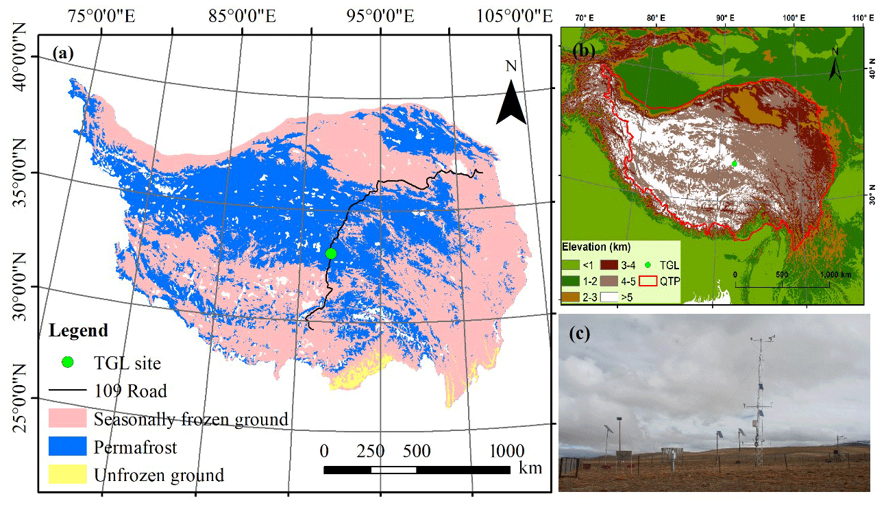
Figure 1Location and geographic features of the study site. (a) Location of the observation site and permafrost distribution (Zou et al., 2017). (b) Topography of the Qinghai–Tibet Plateau. (c) Photo of the Tanggula observation station.
2.2 Ensemble experiments of Noah-MP
The offline Noah-MP LSM v1.1 was assessed in this study. The default Noah-MP model consists of 12 physical processes that are interpreted by multiple optional parameterization schemes. These sub-processes include the following: the vegetation model (VEG), canopy stomatal resistance (CRS), the soil moisture factor for stomatal resistance (BTR), runoff and groundwater (RUN), the surface layer drag coefficient (SFC), supercooled liquid water (FRZ), frozen soil permeability (INF), the canopy gap for radiation transfer (RAD), snow surface albedo (ALB), the precipitation partition (SNF), the lower boundary of soil temperature (TBOT) and the snow/soil temperature time scheme (STC) (Table 1). Details about the processes and optional parameterizations can be found in Yang et al. (2011a).
VEG(1) is adopted in the VEG process, in which the vegetation fraction is prescribed according to the NESDIS/NOAA 0.144 degree monthly 5-year climatology green vegetation fraction (https://ral.ucar.edu/solutions/products/wrf-noah-noah-mp-modeling-system, last access: 27 March 2021), and the monthly leaf area index (LAI) was derived from the Advanced Very High-Resolution Radiometer (AVHRR; https://www.ncei.noaa.gov/data/, last access: 27 March 2021, Claverie et al., 2016). Previous studies have confirmed that Noah-MP seriously overestimates the snow events and underestimates soil temperature and moisture on the QTP (Jiang et al., 2020; Li et al., 2020; Wang et al., 2020), which can be greatly resolved by considering the sublimation from wind (Gordon scheme) and a combination of roughness length for heat and under-canopy (below-canopy) aerodynamic resistance (Y08–UCT scheme) (Zeng et al., 2005; Yang et al., 2008; Li et al., 2020). For a more comprehensive assessment, we added two physical processes based on the default Noah-MP model – i.e., the snow sublimation from wind (SUB) and the combination scheme process (CMB) (Table 1). In the two processes, users can choose to turn on the respective Gordon and Y08–UCT schemes (described in the study of Li et al., 2020) or not. As a result, 55 296 total combinations are possible for the 13 processes, and orthogonal experiments were carried out to evaluate their performance in soil hydrothermal dynamics.
The Noah-MP model was modified to consider the vertical heterogeneity in the soil profile by setting the corresponding soil parameters for each layer. The soil hydraulic parameters, including the porosity, saturated hydraulic conductivity, hydraulic potential, the Clapp–Hornberger parameter b, the field capacity, the wilt point and the saturated soil water diffusivity, were determined using the pedotransfer functions proposed by Hillel (1980), Cosby et al. (1984), and Wetzel and Chang (1987) (Eqs. S1–S7 in the Supplement), in which the sand and clay percentages were based on Hu et al. (2017) (Table S1). In addition, the simulation depth was extended to 8.0 m to cover the active layer thickness of the QTP. The soil column was discretized into 20 layers (Table S1), whose depths follow the default scheme in CLM 5.0 (Lawrence et al., 2018). Due to the inexact match between observed and simulated depths, the simulations at 4, 26, 80, 136, 208 and 299 cm were compared with the observations at 5, 25, 70, 140, 220 and 300 cm, respectively. A 30-year spin-up was conducted in every simulation to reach equilibrium soil states.
Table 1The physical processes and options in the Noah-MP LSM (Yang et al., 2011a).
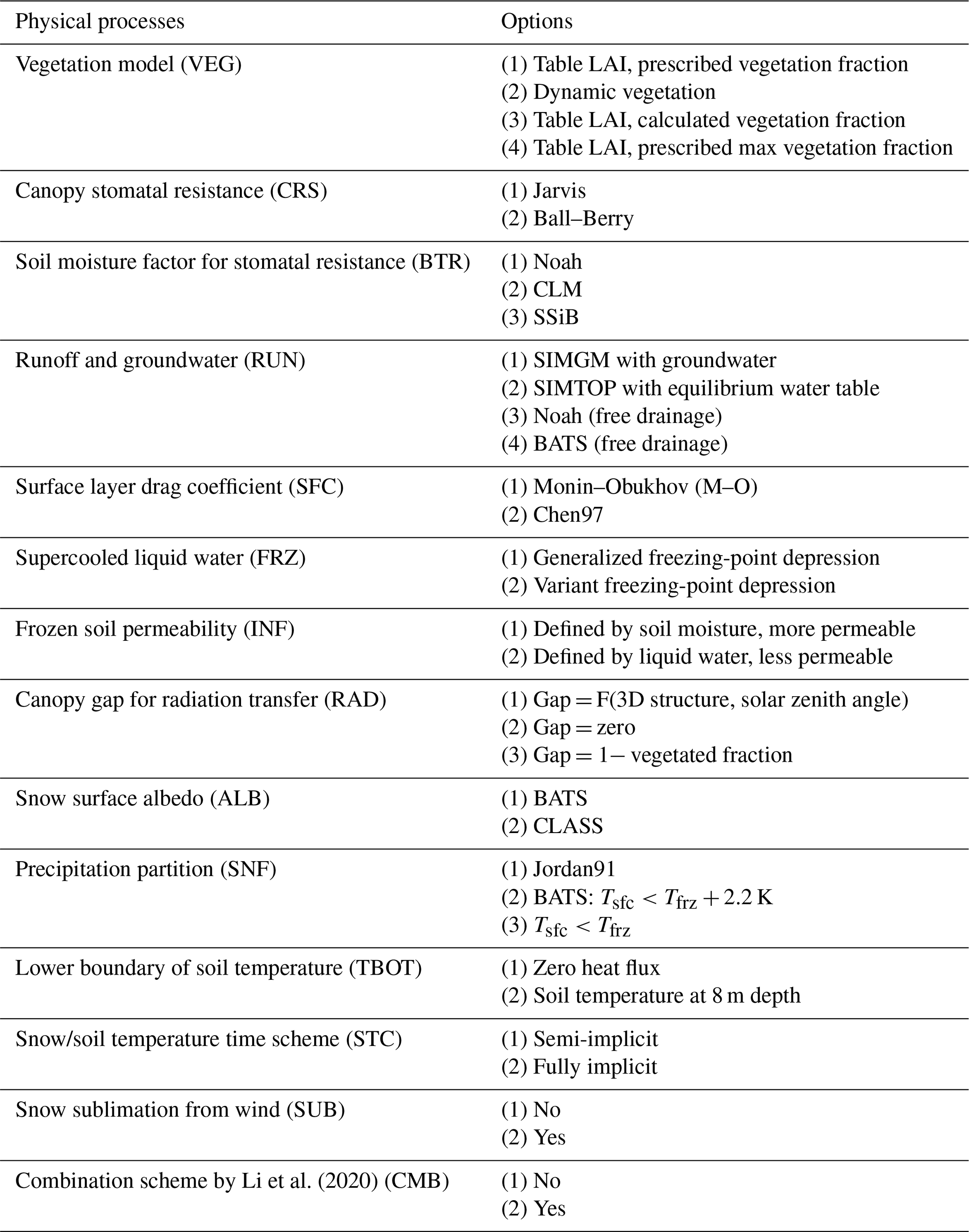
The abbreviations used in the table are as follows: BATS (Biosphere–Atmosphere Transfer Model), CLASS (Canadian Land Surface Scheme), SIMGM (Simple topography-based runoff and Groundwater Model), SIMTOP (Simple Topography-based hydrological model) and SSiB (Simplified Simple Biosphere model).
2.3 Methods for sensitivity analysis
The simulated snow cover events (SCEs) were quantitatively evaluated using the overall accuracy index (OA) (Toure et al., 2016):
where a represents the positive hits, b represents the false alarm, c represents the misses and d represents the negative hits. The value of the OA ranges from 0 to 1. A higher OA signifies better performance. Ground albedo was used as an indicator for snow events due to a lack of snow depth observations. The days when the daily mean albedo is greater than the observed mean value of the warm and cold season (0.25 and 0.30, respectively) are identified as snow cover.
The root mean square errors (RMSEs) between the simulations and observations were adopted to evaluate the performance of Noah-MP in simulating soil hydrothermal dynamics.
To investigate the degree of influence of each physical process on the SCEs, ST and SLW, we firstly calculated the mean OA (for SCE) and the mean RMSE (for ST and SLW) ( of the jth parameterization schemes (j=1, 2, …) in the ith process (i=1, 2, …). The maximum difference in (ΔOA or ΔRMSE) was then defined to quantify the degree of influence of the ith process (i=1, 2, …) (Li et al., 2015):
where and are the largest and the smallest in the ith process, respectively. For a given physical process, a high ΔOA or ΔRMSE signifies a large difference between parameterizations, indicating high sensitiveness of the ith process for SCEs and ST/SLW simulation.
The sensitivities of physical processes were determined by quantifying the statistical distinction level of performance between parameterization schemes. The independent sample (two-tailed) t test was adopted to identify whether the distinction level between two schemes was significant, and the significance of the distinction level between three or more schemes was tested using a Tukey test. The Tukey test has been widely used due to its simple computation and statistical features (Benjamini, 2010). Detailed descriptions of this method can be found in Zhang et al. (2016), Gan et al. (2019) and You et al. (2020a). A process can be considered sensitive when the schemes show a significant difference. Moreover, schemes with a large mean OA and a small mean RMSE were considered favorable for SCEs and ST/SLW simulation, respectively. We distinguished the differences of the parameterization schemes at the 95 % confidence level.
3.1 General performance of the ensemble simulation
The performance of Noah-MP for snow simulation was firstly tested by conducting an ensemble of 55 296 experiments. Due to a lack of snow depth measurements, ground albedo was used as an indicator of snow cover. Figure 2 shows the monthly variations in observed ground albedo and the simulation results of the ensemble simulations. The ground albedo was extremely overestimated with large uncertainties when considering the snow options in Noah-MP, indicating an overestimation of snow depth and duration. This overestimation continued until July.
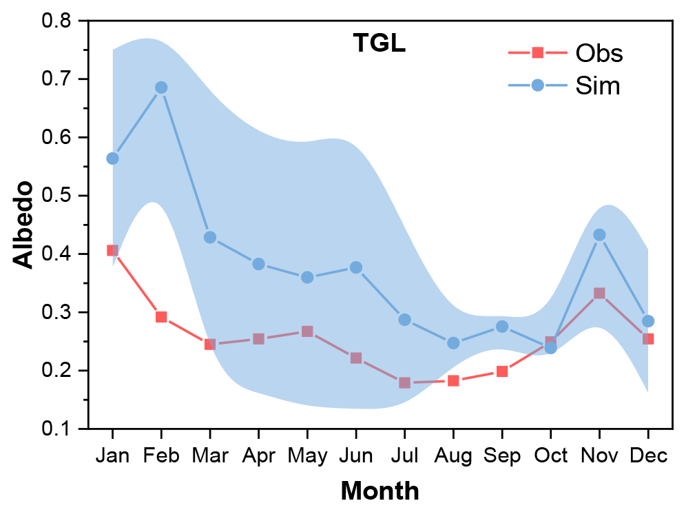
Figure 2Monthly variations in ground albedo at the TGL site for the observations (Obs) and the ensemble simulation (Sim). The light blue shading represents the standard deviation of the ensemble simulation.
Figure 3 illustrates the ensemble-simulated and observed annual cycle of ST and SLW at the TGL site. The ensemble experiments basically captured the seasonal variability of ST, whose magnitude decreased with soil depth. In addition, the simulated ST in the snow-affected season (October–July) showed relatively wide uncertainty ranges, particularly in the shallow layers. This indicates that the selected schemes perform very differently with respect to snow simulation, resulting in large uncertainties in shallow STs. The simulated ST were generally smaller than the observations with relatively large gaps during the snow-affected season. This indicates that the Noah-MP model generally underestimates the ST, especially during the snow-affected months.
As the observation equipment can only record the liquid water, the soil liquid water (SLW) was evaluated against simulations from the ensemble experiments (Fig. 3). The Noah-MP model generally underestimated surface (5 and 25 cm) and deep (220 and 300 cm) SLW (Fig. 3g, h, k, l). However, Noah-MP tended to overestimate the SLW in the middle layers of 70 and 140 cm. Moreover, the simulated SLW exhibited relatively wide uncertainty ranges, particularly during the warm season (Fig. 3).
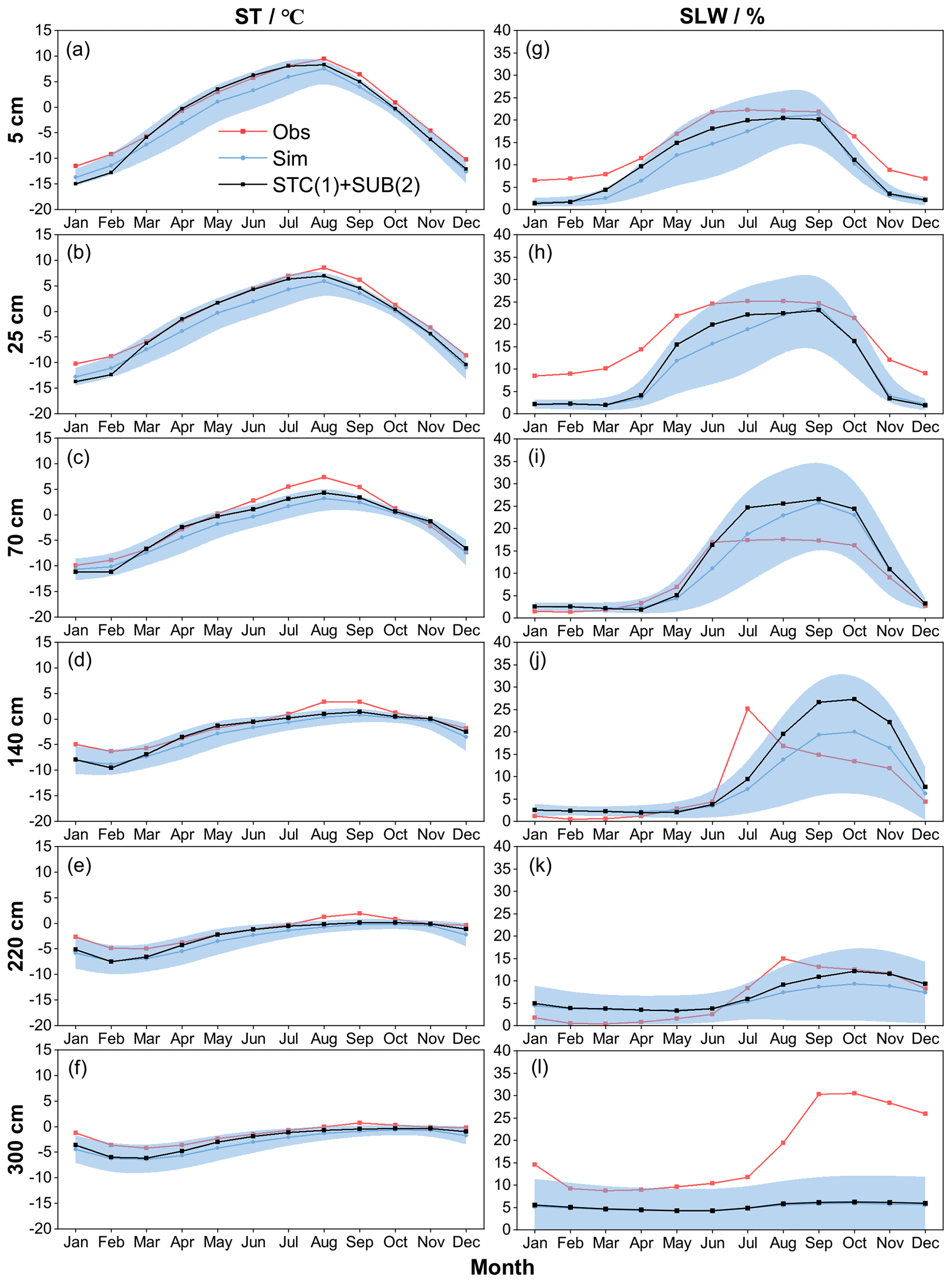
Figure 3Monthly soil temperature (ST, in ∘C) and soil liquid water (SLW, in %) at (a, g) 5 cm, (b, h) 25 cm, (c, i) 70 cm, (d, j) 140 cm, (e, k) 220 cm and (f, l) 300 cm at the TGL site. The light blue shading represents the standard deviation of the ensemble simulation. The black line and the symbols represent the ensemble mean of simulations with STC(1) and SUB(2).

Figure 4The maximum difference in the mean overall accuracy (OA) for albedo (ALB-ΔOA) in each physical process (a) annually and during the (b) cold and (c) warm seasons at the TGL site.
3.2 Sensitivity of physical processes
3.2.1 Degree of influence of physical processes
Figure 4 compares the influence scores of the 13 physical processes based on the maximum difference in the mean OA over 55 296 experiments using the same scheme, for SCEs at the TGL site. On the whole, the SUB and STC processes had the largest scores for the whole year as well as during both the warm and cold seasons, and the other processes showed a value of less than 0.05 (Fig. 4a, b, c). Moreover, the SUB process had a consistent influence on SCEs, whereas the influence of STC differed with season. In the cold season, the score of the SUB process (0.28) was 2 times more than that of the STC process (Fig. 4b), indicating the relative importance of snow sublimation for SCE simulation during the cold season. When it came to the warm season, the influence score of SUB (0.25) did not change much, whereas that of STC increased to 0.26 and showed a similar influence on SCE simulation to SUB.

Figure 5The maximum difference in the mean RMSE for (a, c, e) soil temperature (ST-ΔRMSE, in ∘C) and (b, d, f) soil liquid water (SLW-ΔRMSE, in %) in each physical process (a, b) annually and during the (c, d) warm and (e, f) cold seasons at different soil depths at the TGL site.
Figure 5 compares the influence scores of the 13 physical processes at different soil depths, based on the maximum difference in the mean RMSE over 55 296 experiments using the same scheme, for ST and SLW at the TGL site. The snow-related processes, including the STC, SUB and SNF processes, showed the largest ST-ΔRMSE at all layers, followed by the RAD, SFC and RUN processes, whereas the ST-ΔRMSE values of the other seven physical processes were less than 0.5 ∘C, among which the influence of the CRS and BTR processes were negligible. Moreover, the FRZ, INF and TBOT processes had larger influence scores during the cold season than during the warm season, and the scores of TBOT were greater in deep soils than shallow soils. During the warm season, the physical processes generally showed more influence on shallow soil temperatures. When it came to the cold season, the influence of the physical processes on deep layers obviously increased and was comparable to that on shallow layers, implying relatively higher uncertainties in Noah-MP during the cold season.
Most of the ΔRMSE values for SLW are less than 5 %, indicating that all of the physical processes have limited influence on the SLW, among which CRS, BTR, ALB, SNF and CMB showed the smallest effects (Fig. 5b, d, f). During the warm season, the RUN process, along with the STC and SUB processes, dominated the performance of SLW simulation, especially in the shallow layers (5, 25 and 70 cm; Fig. 5d). During the cold season, however, the RUN process dominated the SLW simulation, with a great decline in the dominance of STC and SUB processes.
3.2.2 Sensitivities of physical processes and the general behaviors of parameterizations
To further investigate the sensitivity of each process and the general performance of the parameterizations, an independent sample (two-tailed) t test and a Tukey test were conducted to establish whether the differences between parameterizations within a physical process were significant (Figs. 6, 7). For a given sub-process, any two schemes labeled with different letters behave significantly differently, and this sub-process can, therefore, be identified as sensitive; otherwise, the sub-process is considered insensitive. For simplicity, schemes with insensitive sub-process are not labeled. Moreover, schemes with the letters late in the alphabet have smaller mean RMSEs and outperform those with letters that appear early in the alphabet. The following outlines an example of this process using the two schemes in the CRS process, hereafter CRS(1) and CRS(2), in Fig. 6. For the annual and warm season, CRS(1) and CRS(2) were labeled with “B” and “A”, respectively. In the cold season, neither of them were labeled with letters. As described above, the CRS process was sensitive for SCE simulation during the annual and warm season, and CRS(1) outperformed CRS(2). However, it was not sensitive during the cold season.
Consistent with the degrees of influence shown in Fig. 4, the performance difference between schemes of the STC and SUB processes for SCE simulation were significantly greater than for other processes. Most other physical processes showed significant but limited differences. Schemes in the BTR and TBOT processes, however, showed no significant difference with respect to performance. Specifically, the performance order was as follows: STC(1) > STC(2), SUB(2) > SUB(1), SFC(2) > SFC(1), ALB(2) > ALB(1) and CMB(2) > CMB(1) at both the annual and seasonal scales. RAD showed no obvious difference during the warm season, whereas RAD(3) outperformed RAD(1) and RAD(2) during the cold season. For SNF, SNF(3) generally excelled over SNF(1) and SNF(2), especially during the warm season.
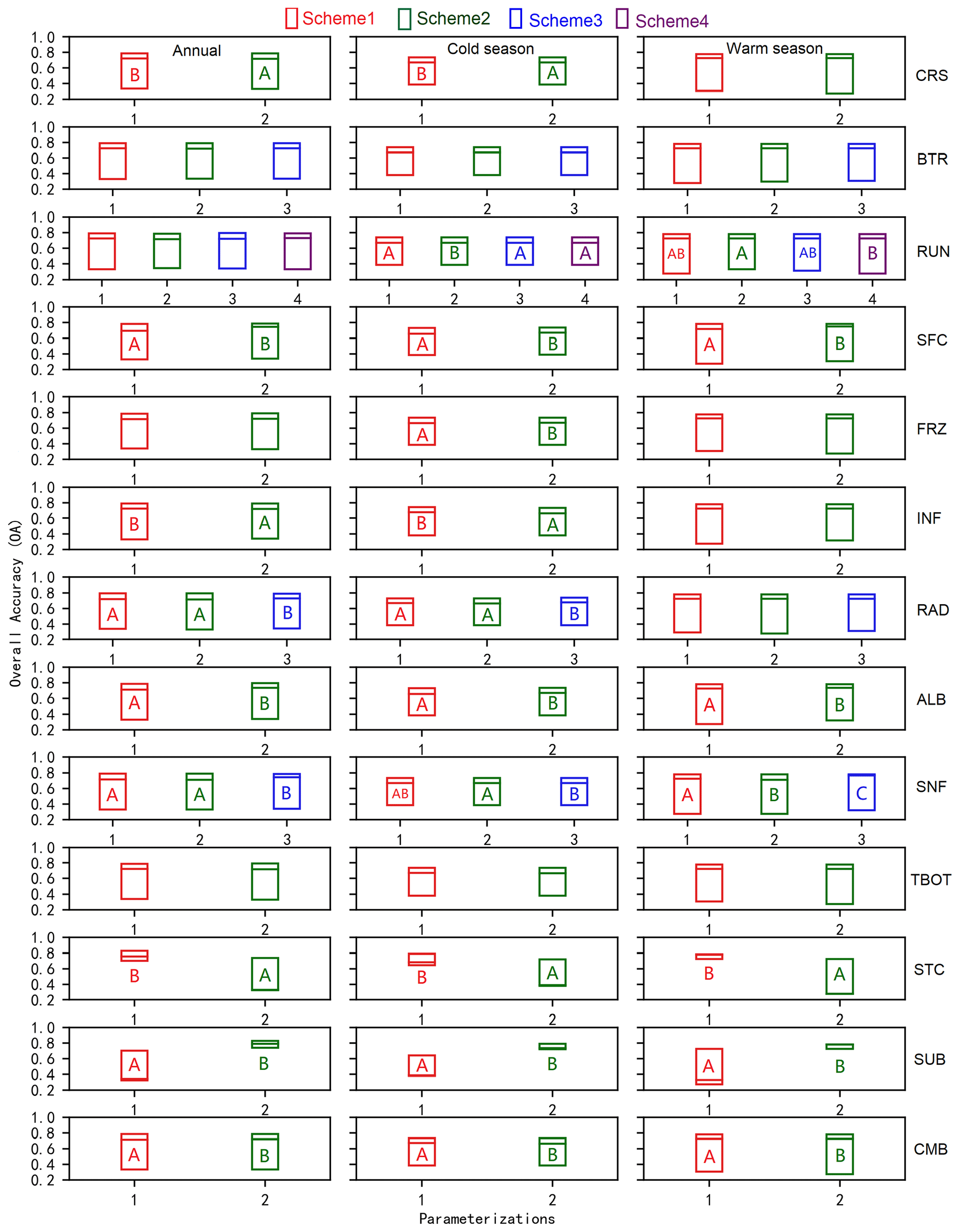
Figure 6Distinction level for overall accuracy (OA) of snow cover events (SCEs) annually and during the warm and cold seasons at the TGL site. The limits of the boxes represent the upper and lower quartiles, and the lines in the boxes indicate the median values.
All of the physical processes showed sensitivities for ST and SLW simulation to varying magnitudes except for the BTR and CRS processes in most layers. For ST, the performance difference between schemes of the STC, SUB and SNF processes were obviously greater than other processes, indicating the importance of snow on ST, followed by the RAD, SFC and RUN processes. The performance order was as follows: STC(1) > STC(2), SUB(2) > SUB(1), SNF(3) > SNF(1) > SNF(2), RAD(3) > RAD(1) > RAD(2) and SFC(2) > SFC(1). For SLW, the RUN, STC and SUB processes showed significant and higher sensitivities than other physical processes, especially during the warm season and in the shallow layers (Figs. 5, 8). Consistent with that of ST, the performance order for the SLW simulation was as follows: STC(1) > STC(2) and SUB(2) > SUB(1). For the RUN process, the performance order for both ST and SLW simulation generally followed RUN(4) > RUN(1) > RUN(3) > RUN(2) as a whole, among which RUN(1) and RUN(4) showed similar performance during both warm and cold seasons. During both warm and cold seasons, the performance order for the ST simulations was SFC(2) > SFC(1) for SFC process, FRZ(2) > FRZ(1) for FRZ process and RAD(3) > RAD(1) > RAD(2) for RAD process (Figs. S2, S3), which is somewhat similar to SLW simulations in the shallow and deep layers.
For ST, both FRZ and INF showed higher sensitivities during the cold season, especially in shallow soils for FRZ and deep soils for INF. FRZ(2) INF(1) outperformed FRZ(1) INF(2) for the whole year with respect to ST simulation. Specifically, FRZ(1) INF(2) performed better in shallow soils during the warm season, whereas its performance was worse during the cold season compared with FRZ(2) INF(1). For SLW, FRZ(2) INF(2) generally preceded FRZ(1) INF(1) in shallow and deep soils (5, 25, 220 and 300 cm), whereas its performance was worse in the middle soil layers (140 and 220 cm).
For ST simulation, the performance sequence for RAD and SNF was RAD(3) > RAD(1) > RAD(2) and SNF(3) > SNF(1) > SNF(2), respectively. For SLW simulation, the sequence became complicated. However, RAD(3) and SNF(3) still outperformed the other two schemes, respectively. ALB(2) was superior to ALB(1) for both ST and SLW simulation. The influence of TBOT on soil hydrothermal dynamics arose in deep soils and during cold season, and TBOT(1) excelled over TBOT(2). CMB(2) outperformed CMB(1) for ST simulation and for SLW simulation in shallow and deep soils (5, 25 and 300 cm).
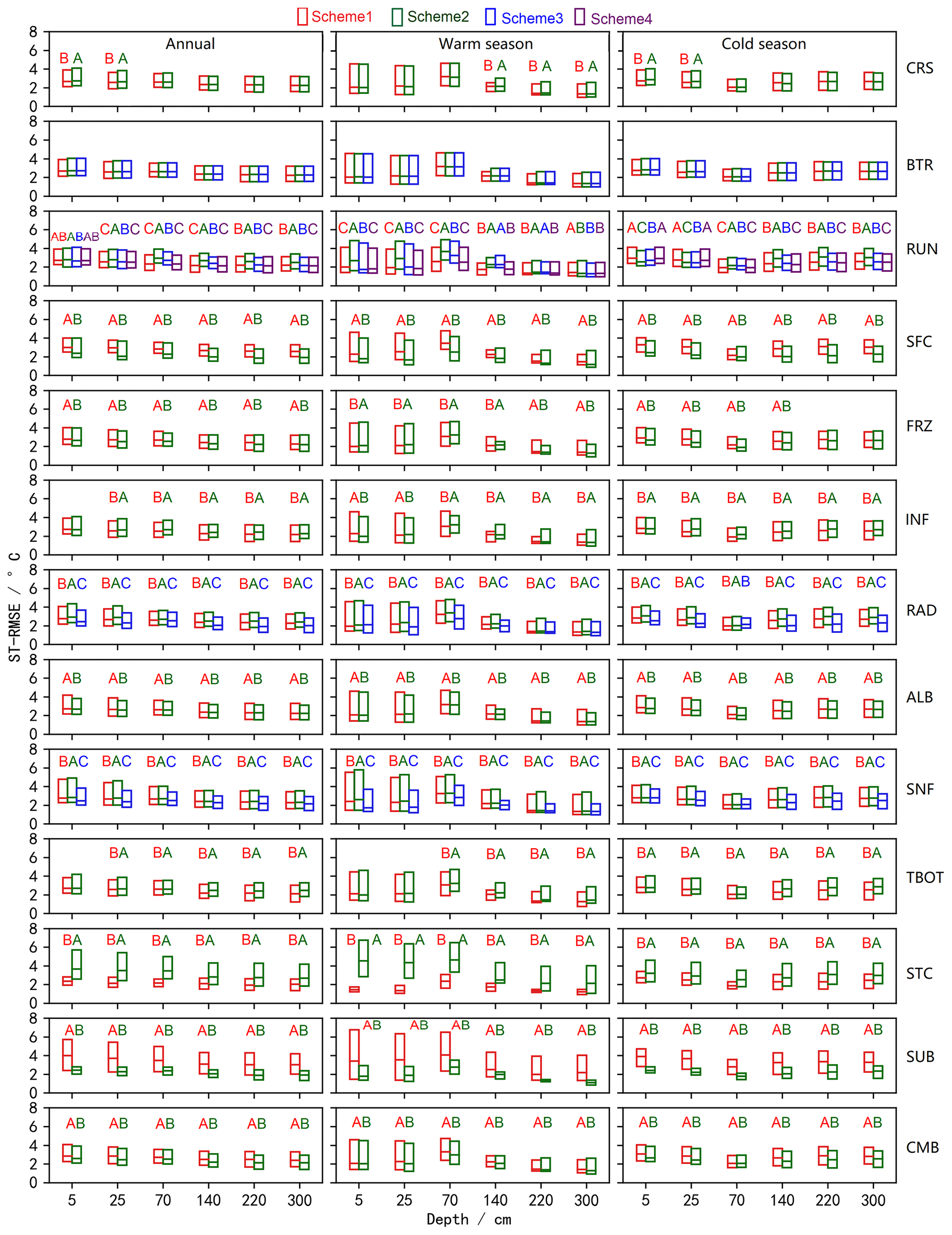
Figure 7Distinction level for the RMSE of ST at different layers annually and during the warm and cold seasons in the ensemble simulations at the TGL site. Limits of the boxes represent the upper and lower quartiles, and the lines in the boxes indicate the median values.

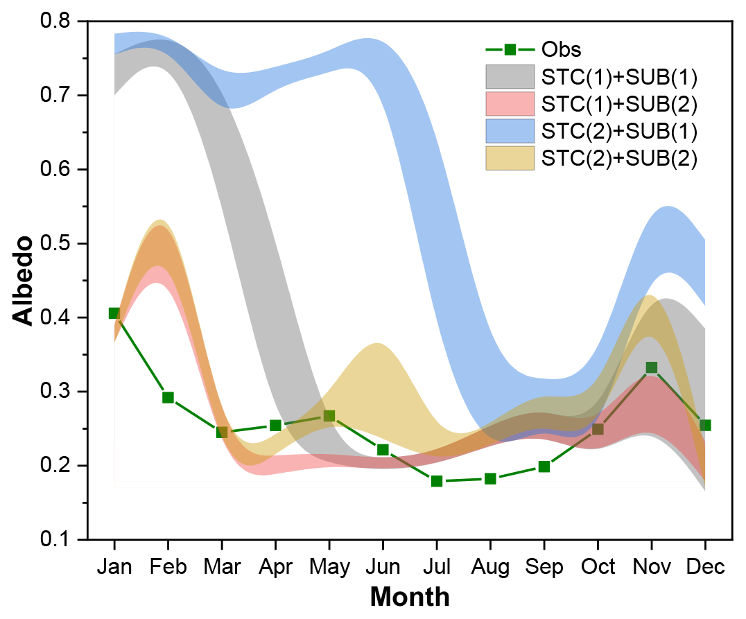
Figure 9Uncertainty interval of ground albedo at the TGL site in the dominant physical processes (STC and SUB) for SCE simulation.
3.3 Influence of snow cover and the surface drag coefficient on soil hydrothermal dynamics
The influence of snow on soil temperature is firstly investigated. The dominant role of STC and SUB in the simulation of SCEs has been identified (Figs. 4, 6). Interactions between the two physical processes are further analyzed here. Figure 9 compares the uncertainly intervals of the two physics. The duration of snow cover is the longest when STC(2) + SUB(1), followed by when STC(1) + SUB(1). Simulations considering SUB(2) generally have a short snow duration. Among the four combinations, STC(1) + SUB(2) is in best agreement with the measurements.
Given the good performance of STC(1) + SUB(2) in simulating SCEs, the influence of snow on soil hydrothermal dynamics is investigated by comparing the total ensemble mean ST and SLW with those adopting STC(1) + SUB(2) (Fig. 3). It can be seen that the ensemble mean ST values of simulations adopting STC(1) and SUB(2) are generally higher than the total ensemble means, especially during the spring and summer (March–August). In January and February in the shallow layers (5, 25 and 70 cm), STC(1) + SUB(2) had a lower ST and showed an insulation effect on ST for these 2 months. As a whole, however, snow cover has a cooling effect on ST. In addition, along with the improved SCEs and elevated ST, STC(1) + SUB(2) induced moister soil with a higher SLW (Fig. 3).
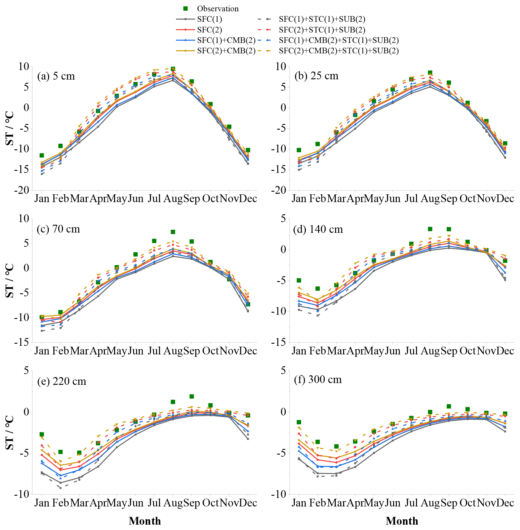
Figure 10Monthly soil temperature (ST, in ∘C) at (a) 5 cm, (b) 25 cm, (c) 70 cm, (d) 140 cm, (e) 220 cm and (f) 300 cm for the SFC process with or without consideration of the CMB(2) and STC(1) + SUB(2) processes.
The SFC and CMB processes use different ways of calculating the surface drag coefficient, which greatly influences the surface energy partitioning and, thus, the ST and SLW. The influence of the surface drag coefficient is assessed by comparing the soil temperature before and after considering the combined scheme, CMB(2), and the effect of snow, STC(1) + SUB(2) (Fig. 10). SFC(2) tended to produce a higher ST than SFC(1), especially during the warming period (January–August). When adopting the combined Y08–UCT scheme, CMB(2), the cold bias was significantly resolved. The performance order was as follows: SFC(2) + CMB(2) > SFC(2) > SFC(1) + CMB(2) > SFC(1). However, considerable underestimations of ST still exist in all layers due to the poor representation of snow process. After eliminating the effects of snow (STC(1) + SUB(2), dash lines in Fig. 10), the simulated ST increased accordingly, except in January and February. SFC(2) and SFC(2) + CMB(2) overestimated STs from March to July in the shallow layers (5 and 25 cm), resulting in good agreement of deep STs with observations. In contrast, the simulated STs in the shallow layers (5 and 25 cm) by SFC(1) and SFC(1) + CMB(2) were basically consistent with observations from March to July, whereas a large cold bias remained in the deep layers.
4.1 Snow cover on the QTP and its influence on the soil hydrothermal regime
Snow cover in the permafrost regions of the QTP is thin, patchy and short-lived (Che et al., 2019), and its influence on soil temperature and the permafrost state is usually considered weak (Jin et al., 2008; Zou et al., 2017; Wu et al., 2018; Zhang et al., 2018; Yao et al., 2019). However, our ensemble simulations showed that the surface albedo is extremely overestimated with respect to both magnitude and duration (Fig. 2), implying an extreme overestimation of snow cover, which is consistent with studies using Noah-MP model (Jiang et al., 2020; Li et al., 2020; Wang et al., 2020) and widely found in other state-of-the-art LSMs (Wei and Dong, 2015) for the QTP.
Great efforts to resolve the overestimation of snow cover in LSMs include considering the vegetation effect (Park et al., 2016), the snow cover fraction (Jiang et al., 2020), blowing snow (Xie et al., 2019) and the fresh snow albedo (Wang et al., 2020). Our results illustrated the superiority of considering the snow sublimation from wind (SUB(2)) and using a semi-implicit snow/soil temperature time scheme (STC(1)) (Figs. 4, 6, 9) when simulating snow cover on the QTP. This is consistent with previous conclusions that accounting for the loss resulting from wind contributes to improving the snow cover days and depth (Yuan et al., 2016) and that STC(1) has more rapid snow ablation than STC(2) (You et al., 2020a).
The impacts of snow cover on soil temperature with respect to magnitude and vector (cooling or warming) depend on its timing, duration and depth (Zhang et al., 2005). In January and February, the ground heat flux mainly goes upward, and the warming effect of simulated snow can be related to the overestimated snow depth that prevents heat loss from the ground. During the spring and summer, when snow melts, a cooling effects occurs, mainly because the considerable energy that is used to heat the ground is reflected due to the high albedo of snow. With the improvement of snow (STC(1) + SUB(2)), the originally overestimated snow melts and infiltrates into the soil, resulting in improved SLWs (Fig. 3). A higher soil temperature also contributed to the SLWs according to the freezing-point depression equation, in which SLW exponentially increases with soil temperature for a given site (Niu and Yang, 2006).
4.2 Discussions on the sensitivity of physical processes to soil hydrothermal simulation
4.2.1 Canopy stomatal resistance (CRS) and soil moisture factor for stomatal resistance (BTR)
The biophysical BTR and CRS processes directly affect the canopy stomatal resistance and, thus, plant transpiration (Niu et al., 2011). The transpiration of plants could impact the ST and SLW through its cooling effect (Shen et al., 2015) and the water balance in the root zone (Chang et al., 2020). However, the annual transpiration of the alpine steppe is weak due to the shallow effective root zone and lower stomatal control in this dry environment (Ma et al., 2015), which may explain the indistinctive or very small difference among the schemes of the BTR and CRS processes for SCEs (Fig. 6), ST (Fig. 7) and SLW (Fig. 8).
4.2.2 Runoff and groundwater (RUN)
In the warm season, different SLWs would result in a difference in the surface energy partitioning and, thus, different soil temperatures. RUN(2) had the worst performance for simulating ST and SLW (Figs. 7, 8) among the four schemes, likely due to its higher estimation of soil moisture (Fig. S1) and, thus, greater sensible heat and smaller ST (Gao et al., 2015). Likewise, RUN(4) was on par with RUN(1) with respect to the simulation of ST in most layers due to the very small difference in the SLW of the two schemes (Figs. 8, S1). For the whole soil column, RUN(4) surpassed RUN(1) and RUN(2) for SLW simulation, both of which define surface and subsurface runoff as functions of the groundwater table depth (Niu et al., 2005, 2007). This is in keeping with the study of Zheng et al. (2017), which found that soil-water-storage-based parameterizations outperformed groundwater-table-based parameterizations in simulating the total runoff in a seasonally frozen and high-altitude Tibetan river. Moreover, RUN(4) is designed based on the infiltration-excess runoff (Yang and Dickinson, 1996) in spite of the saturation-excess runoff in RUN(1) and RUN(2) (Gan et al., 2019), which is more common in arid and semiarid areas like the permafrost regions of the QTP (Pilgrim et al., 1988). In the cold season, much of the liquid water freezes into ice, which would greatly influence the thermal conductivity of frozen soil considering that the thermal conductivity of ice is nearly 4 times that of the equivalent liquid water. Therefore, the impact of RUN is important for the soil temperature simulations in both the warm and cold seasons (Figs. 5, 7).
4.2.3 Surface layer drag coefficient (SFC and CMB)
SFC defines the calculation of the surface exchange coefficient for heat and water vapor (CH), which greatly impact the energy and water balance and, thus, the temperature and moisture of soil (Zeng et al., 2012; Zheng et al., 2012). SFC(1) adopts the Monin–Obukhov similarity theory (MOST) in its general form, whereas SFC(2) uses the improved MOST modified by Chen et al. (1997). In SFC(1), the roughness length for heat (Z0h) is taken as the same as the roughness length for momentum (Z0m; Niu et al., 2011). SFC(2) adopts the Zilitinkevich approach for Z0h calculation (Zilitinkevich, 1995). The difference between SFC(1) and SFC(2) has a great impact on the CH value. Several studies have reported that SFC(2) shows better performance for the simulation of sensible and latent heat on the QTP (Zhang et al., 2016; Gan et al., 2019). The results of the t test in this study showed remarkable distinctions between the two schemes, where SFC(2) was dramatically superior to SFC(1) (Figs. 7, 8). SFC(2) produces lower CH values than SFC(1) (Zhang et al., 2014), resulting in less efficient ventilation and greater heating of the land surface (Yang et al., 2011b) as well as a substantial improvement in the cold bias of Noah-MP in this study (Figs. 7, 10).
Both SFC(1) and SFC(2) could not produce the diurnal variation in Z0h (Chen et al., 2010). CMB offers a scheme that considers the diurnal variation in Z0h in bare ground and under-canopy turbulent exchange in sparse vegetated surfaces (Li et al., 2020). Consistent with previous studies on the QTP (Chen et al., 2010; Guo et al., 2011; Zheng et al., 2015; Li et al., 2020), the simulated ST generally followed SFC(2) + CMB(2) > SFC(2) > SFC(1) + CMB(2) > SFC(1) with/without removing the overestimation of snow (Fig. 10), indicating that CMB(2) contributes to resolving the cold bias of the LSMs. However, none of the four combinations could satisfactorily reproduce the shallow and deep STs simultaneously. When the snow was well-simulated, SFC(2) + CMB(2) performed the best in the deep layers at the cost of overestimating the shallow STs. Meanwhile, SFC(1) + CMB(1) showed the best agreement in the shallow layers with a considerable cold bias in the deep layers, which could be related to the overestimated frozen soil thermal conductivity (Luo et al., 2009; Chen et al., 2012; Li et al., 2019).
4.2.4 Supercooled liquid water (FRZ) and frozen soil permeability (INF)
FRZ and INF describe the unfrozen water and permeability of frozen soil, and they had a larger influence on ST and SLW during the cold season than during the warm season, as expected (Fig. 5). Specifically, FRZ treats liquid water in frozen soil (supercooled liquid water) using two forms of the freezing-point depression equation. FRZ(1) takes a general form (Niu and Yang, 2006), whereas FRZ(2) exhibits a variant form that considers the increased surface area of icy soil particles (Koren et al., 1999). FRZ(2) generally yields more liquid water compared with FRZ(1) (Fig. S2). INF(1) uses soil moisture (Niu and Yang, 2006), whereas INF(2) employs only the liquid water (Koren et al., 1999) to parameterize soil hydraulic properties. INF(2) generally produces more impermeable frozen soil than INF(1), which is also found in this study (Fig. S3). For the whole year, INF(1) surpassed INF(2) with respect to simulating STs, which may be related to the more realistic SLWs produced by INF(1) for the whole soil column (Fig. S3).
4.2.5 Canopy gap for radiation transfer (RAD)
RAD treats the radiation transfer process within the vegetation and adopts three methods to calculate the canopy gap. RAD(1) defines the canopy gap as a function of the 3D vegetation structure and the solar zenith angle, RAD(2) employs no gap within canopy and RAD(3) treats the canopy gap from unity minus the vegetation fraction (Niu and Yang, 2004). The RAD(3) scheme allows the most solar radiation to penetrate to the ground, followed by the RAD(1) and RAD(2) schemes. As it is an alpine grassland, there is a relative low LAI at the TGL site and, thus, quite a high canopy gap. Therefore, schemes with a larger canopy gap could realistically reflect the environment. Consequently, the performance decreased in the following order for the ST and SLW simulation: RAD(3) > RAD(1) > RAD(2).
4.2.6 Snow surface albedo (ALB) and precipitation partition (SNF)
The ALB describes two ways of calculating snow surface albedo, in which ALB(1) and ALB(2) adopt the scheme from the BATS and CLASS LSMs, respectively. ALB(2) generally produces lower albedo than ALB(1), especially when the ground is covered by snow (Fig. S4). As a result, higher net radiation is absorbed by the land surface and more heat is available for heating the soil in ALB(2), which is beneficial for counteracting the cooling effect of overestimated snow on the ST (Fig. S5). Along with the higher ST, ALB(2) outperformed ALB(1) with respect to SLW simulation, likely due to more snowmelt water offsetting the dry bias in Noah-MP (Fig. S5).
The SNF defines the snowfall fraction of precipitation as a function of surface air temperature. SNF(1) is the most complicated of the three schemes, in which the precipitation is considered rain (snow) when the surface air temperature is greater (less) than or equal to 2.5 ∘C (0.5 ∘C), otherwise it is recognized as sleet, whereas SNF(2) and SNF(3) simply distinguish rain or snow by judging whether the air temperature is above the respective thresholds of 2.2 and 0 ∘C or not. The significant difference between the three schemes for SCE simulation during the warm season is consistent with the large difference in the snowfall fraction in this period (Figs. 6, S6). SNF(3) is the most rigorous scheme and produces the minimum amount of snow, followed by SNF(1) and SNF(2) with limited difference (Fig. S6). This specifically explains the superiority of SNF(3) for ST and SLW simulation (Figs. 7, 8).
4.2.7 Lower boundary of soil temperature (TBOT) and the snow/soil temperature time scheme (STC)
The TBOT process adopts two schemes to describe the soil temperature boundary conditions. TBOT(1) assumes zero heat flux at the bottom of the model, whereas TBOT(2) adopts the soil temperature at 8 m depth (Yang et al., 2011a). In general, TBOT(1) is expected to accumulate heat in the deep soil and produce higher ST than TBOT(2). In this study, the two assumptions performed significantly differently, especially in the deep soil layers and during the cold season. Although TBOT(2) is more representative of realistic conditions, TBOT(1) surpassed TBOT(2) in this study. This can be related to the overall underestimation in the model, which can be alleviated by TBOT(1) due to heat accumulation (Fig. S7).
Two time discretization strategies are implemented in the STC process – STC(1) adopts the semi-implicit scheme, whereas STC(2) uses the fully implicit scheme – to solve the thermal diffusion equation in first soil or snow layers (Yang et al., 2011a). STC(1) and STC(2) are not strictly physical processes, they are different upper boundary conditions of the soil column (You et al., 2020a). The differences between STC(1) and STC(2) were significant (Fig. 7). The impacts of the two options on ST are remarkable (Fig. 6), particularly in the shallow layers and during the warm season (Fig. 5). In addition, STC(1) outperformed STC(2) in the ensemble-simulated ST (Fig. 7), because STC(1) greatly alleviated the cold bias in Noah-MP (Fig. S8) by producing a higher OA for SCEs (Fig. 6).
4.3 Perspectives
This study analyzed the characteristics and general behavior of each parameterization scheme of Noah-MP at a typical permafrost site on the QTP, hoping to provide a reference for simulating the permafrost state on the QTP. We identified the systematic overestimation of snow cover, cold bias and dry bias in Noah-MP, and discussed the role of snow and the surface drag coefficient on soil hydrothermal dynamics. Further tests at another permafrost site (BLH site; 34.82∘ N, 92.92∘ E; 4,659 m a.s.l.) basically showed consistent conclusions with those from the TGL site (see the Supplement for details), indicating that relevant results and methodologies can be practical guidelines for improving the parameterizations of physical processes and testing their uncertainties towards soil hydrothermal modeling in the permafrost regions of the plateau. Although the site that we selected may be representative of the typical environment on the plateau, continued investigation with a broad spectrum of climate and environmental conditions is required to make a general conclusion at a regional scale.
An ensemble simulation using multi-parameterizations was conducted using the Noah-MP model at the TGL site, aiming to present a reference for simulating soil hydrothermal dynamics in the permafrost regions of the QTP using LSMs. The model was modified to consider the vertical heterogeneity in the soil, and the simulation depth was extended to cover the whole active layer. The ensemble simulation consists of 55 296 experiments, combining 13 physical processes (CRS, BTR, RUN, SFC, FRZ, INF, RAD, ALB, SNF, TBOT, STC, SUB and CMB), each with multiple optional schemes. On this basis, the general performance of Noah-MP was assessed by comparing simulation results with in situ observations, and the sensitivity of snow cover event, soil temperature and moisture at different depths of the active layer to the parameterization schemes was explored. The main conclusions of the study are as follows:
-
Noah-MP tends to overestimate snow cover, which is most influenced by the STC and SUB processes. Such overestimation can be greatly resolved by considering the snow sublimation from wind, SUB(2) and the semi-implicit snow/soil temperature time scheme, STC(1).
-
Soil temperature is largely underestimated by the overestimated snow cover and, thus, dominated by the STC and SUB processes. Systematic cold bias and large uncertainties in soil temperature still exist after eliminating the effects of snow, particularly in the deep layers and during the cold season. The combination of the Y08 and UCT schemes contributes to resolving the cold bias of soil temperature.
-
Noah-MP tends to underestimate the soil liquid water content. Most physical processes have a limited influence on the soil liquid water content, among which the RUN process plays a dominant role during the whole year. The STC and SUB process have a considerable influence on topsoil liquid water during the warm season.
The original source code of the offline 1D Noah-MP LSM v1.1 is available at https://ral.ucar.edu/solutions/products/noah-multiparameterization-land-surface-model-noah-mp-lsm (last access: 23 February 2021). The modified Noah-MP LSM considering vertical heterogeneity in the soil profile, snow sublimation from wind, and the combination of roughness length for heat and under-canopy aerodynamic resistance can be downloaded from https://doi.org/10.5281/zenodo.4555449 (Li, 2021).
The 1-hourly forcing data, daily soil temperature and liquid water content at the TGL and BLH sites are available at https://doi.org/10.17632/h7hbd69nnr.2 (Li, 2020). Soil texture data can be obtained from https://doi.org/10.1016/j.catena.2017.04.011 (Hu et al., 2017). The AVHRR LAI data can be downloaded from https://www.ncei.noaa.gov/data/ (last access: 27 March 2021, Claverie et al., 2016).
The supplement related to this article is available online at: https://doi.org/10.5194/gmd-14-1753-2021-supplement.
TW and XL conceived the idea and designed the model experiments. XL performed the simulations, analyzed the output and wrote the paper. JC helped to compile the model in a GNU/Linux (CentOS 7.0) environment. XW, XZ, GH and RL contributed to conducting the simulation and interpreting the results. YQ provided the observations of atmospheric forcing and soil temperature. CY and JH helped with downloading and processing the AVHRR LAI data. JN and WM provide guidelines for the visualization. All authors revised and polished the paper.
The authors declare that they have no conflict of interest.
The authors thank the Cryosphere Research Station on the Qinghai–Tibet Plateau, CAS, for providing field observation data and Guohui Zhao for providing access to supercomputing resources. The authors are also grateful to Sizhong Yang and the two anonymous reviewers for their insightful and constructive comments and suggestions that greatly improved the quality of the paper.
This research has been supported by the CAS “Light of West China” program, the National Natural Science Foundation of China (grant nos. 41690142, 41771076, 41961144021 and 42071093), the CAS “Hundred Talents program” (Sizhong Yang) and the National Cryosphere Desert Data Center Program (grant no. E0510104).
This paper was edited by Juan Antonio Añel and reviewed by two anonymous referees.
Benjamini, Y.: Simultaneous and selective inference: Current successes and future challenges, Biometrical J., 52, 708–721, https://doi.org/10.1002/bimj.200900299, 2010.
Cao, B., Zhang, T., Wu, Q., Sheng, Y., Zhao, L., and Zou, D.: Brief communication: Evaluation and inter-comparisons of Qinghai–Tibet Plateau permafrost maps based on a new inventory of field evidence, The Cryosphere, 13, 511–519, https://doi.org/10.5194/tc-13-511-2019, 2019.
Chang, M., Liao, W., Wang, X., Zhang, Q., Chen, W., Wu, Z., and Hu, Z.: An optimal ensemble of the Noah-MP land surface model for simulating surface heat fluxes over a typical subtropical forest in South China, Agr. Forest Meteorol., 281, 107815, https://doi.org/10.1016/j.agrformet.2019.107815, 2020.
Che, T., Hao, X., Dai, L., Li, H., Huang, X., and Xiao, L.: Snow cover variation and its impacts over the Qinghai-Tibet Plateau, B. Chin. Acad. Sci., 34, 1247–1253, https://doi.org/10.16418/j.issn.1000-3045.2019.11.007, 2019.
Chen, F., Janjić, Z., and Mitchell, K.: Impact of atmospheric surface-layer parameterizations in the new land-surface scheme of the NCEP Mesoscale Eta Model, Bound.-Lay. Meteorol. 85, 391–421, https://doi.org/10.1023/A:1000531001463, 1997.
Chen, R., Yang, M., Wang, X., and Wan, G.: Review on simulation of land-surface processes on the Tibetan Plateau, Sci. Cold Arid Reg., 11, 93–115, 2019.
Chen, S., Li, X., Wu, T., Xue, K., Luo, D., Wang, X., Wu, Q., Kang, S., Zhou, H., and Wei, D.: Soil thermal regime alteration under experimental warming in permafrost regions of the central Tibetan Plateau, Geoderma, 372, 114397, https://doi.org/10.1016/j.geoderma.2020.114397, 2020.
Chen, Y., Yang, K., Zhou, D., Qin, J., and Guo, X.: Improving the Noah land surface model in arid regions with an appropriate parameterization of the thermal roughness length, J. Hydrometeor., 11, 995–1006, https://doi.org/10.1175/2010JHM1185.1, 2010.
Chen, Y., Yang, K., Tang, W., Qin, J., and Zhao, L.: Parameterizing soil organic carbon's impacts on soil porosity and thermal parameters for Eastern Tibet grasslands, Sci. Chin. Earth Sci., 55, 1001–1011, https://doi.org/10.1007/s11430-012-4433-0, 2012.
Claverie, M., Matthews, J. L., Vermote, E. F., and Justice, C. O.: A 30+ year AVHRR LAI and FAPAR climate data record: Algorithm description and validation, Remote Sens., 8, 263, https://doi.org/10.3390/rs8030263, 2016.
Cosby, B. J., Hornberger, G. M., Clapp, R. B., and Ginn, T. R.: A statistical exploration of the relationships of soil moisture characteristics to the physical properties of soils, Water Resour. Res., 20, 682–690, https://doi.org/10.1029/WR020i006p00682, 1984.
Daniel, R., Nikolay, S., Bernd, E., Stephan, G., and Sergei, M.: Recent advances in permafrost modelling, Permafr. Periglac. Process., 19, 137–156, https://doi.org/10.1002/ppp.615, 2008.
Fountain, A. G., Campbell, J. L., Schuur, E. A. G., Stammerjohn, S. E., Williams, M. W., and Ducklow, H. W.: The disappearing cryosphere: Impacts and ecosystem responses to rapid cryosphere loss, BioScience, 62, 405–415, https://doi.org/10.1525/bio.2012.62.4.11, 2012.
Gan, Y. J., Liang, X. Z., Duan, Q. Y., Chen, F., Li, J. D., and Zhang, Y.: Assessment and reduction of the physical parameterization uncertainty for Noah-MP land surface model, Water Resour. Res., 55, 5518–5538, https://doi.org/10.1029/2019wr024814, 2019.
Gao, Y., Kai, L., Fei, C., Jiang, Y., and Lu, C.: Assessing and improving Noah-MP land model simulations for the central Tibetan Plateau, J. Geophys. Res.-Atmos., 120, 9258–9278, https://doi.org/10.1002/2015JD023404, 2015.
Guo, D. and Wang, H.: Simulation of permafrost and seasonally frozen ground conditions on the Tibetan Plateau, 1981–2010, J. Geophys. Res.-Atmos., 118, 5216–5230, https://doi.org/10.1002/jgrd.50457, 2013.
Guo, X., Yang, K., Zhao, L., Yang, W., Li, S., Zhu, M., Yao, T., and Chen, Y.: Critical evaluation of scalar roughness length parametrizations over a melting valley glacier, Bound.-Lay. Meteorol., 139, 307–332, https://doi.org/10.1007/s10546-010-9586-9, 2011.
He, K., Sun, J., and Chen, Q.: Response of climate and soil texture to net primary productivity and precipitation-use efficiency in the Tibetan Plateau, Pratacultural Sci., 36, 1053–1065, 2019.
Hillel, D.: Applications of Soil Physics, Academic Press, New York, 400 pp., 1980.
Hjort, J., Karjalainen, O., Aalto, J., Westermann, S., Romanovsky, V. E., Nelson, F. E., Etzelmüller, B., and Luoto, M.: Degrading permafrost puts Arctic infrastructure at risk by mid-century, Nat. Commun., 9, 5147, https://doi.org/10.1038/s41467-018-07557-4, 2018.
Hong, S., Yu, X., Park, S. K., Choi, Y.-S., and Myoung, B.: Assessing optimal set of implemented physical parameterization schemes in a multi-physics land surface model using genetic algorithm, Geosci. Model Dev., 7, 2517–2529, https://doi.org/10.5194/gmd-7-2517-2014, 2014.
Hu, G., Zhao, L., Li, R., Wu, T., Wu, X., Pang, Q., Xiao, Y., Qiao, Y., and Shi, J.: Modeling hydrothermal transfer processes in permafrost regions of Qinghai-Tibet Plateau in China, Chin. Geograph. Sci., 25, 713–727, https://doi.org/10.1007/s11769-015-0733-6, 2015.
Hu, G., Zhao, L., Wu, X., Li, R., Wu, T., Xie, C., Pang, Q., and Zou, D.: Comparison of the thermal conductivity parameterizations for a freeze-thaw algorithm with a multi-layered soil in permafrost regions, Catena, 156, 244–251, https://doi.org/10.1016/j.catena.2017.04.011, 2017.
Jiang, Y., Chen, F., Gao, Y., He, C., Barlage, M., and Huang, W.: Assessment of uncertainty sources in snow cover simulation in the Tibetan Plateau, J. Geophys. Res.-Atmos., 125, e2020JD032674, https://doi.org/10.1029/2020JD032674, 2020.
Jin, H., Sun, L., Wang, S., He, R., Lu, L., and Yu, S.: Dual influences of local environmental variables on ground temperatures on the interior-eastern Qinghai-Tibet Plateau (I): vegetation and snow cover, J. Glaciol. Geocryol., 30, 535–545, 2008.
Koren, V., Schaake, J., Mitchell, K., Duan, Q. Y., Chen, F., and Baker, J. M.: A parameterization of snowpack and frozen ground intended for NCEP weather and climate models, J. Geophys. Res.-Atmos., 104, 19569–19585, https://doi.org/10.1029/1999JD900232, 1999.
Koven, C., Riley, W., and Stern, A.: Analysis of permafrost thermal dynamics and response to climate change in the CMIP5 earth system models, J. Climate, 26, 1877–1900, https://doi.org/10.1175/JCLI-D-12-00228.1, 2013.
Lawrence, D., Fisher, R., Koven, C., Oleson, K., Swenson, S., and Vertenstein, M.: Technical description of version 5.0 of the Community Land Model (CLM), National Center for Atmospheric Research, Boulder, Colorado, 2018.
Li, K., Gao, Y., Fei, C., Xu, J., Jiang, Y., Xiao, L., Li, R., and Pan, Y.: Simulation of impact of roots on soil moisture and surface fluxes over central Qinghai–Xizang Plateau, Plateau Meteor., 34, 642–652, https://doi.org/10.7522/j.issn.1000-0534.2015.00035, 2015.
Li, R., Zhao, L., Wu, T., Wang, Q. X., Ding, Y., Yao, J., Wu, X., Hu, G., Xiao, Y., Du, Y., Zhu, X., Qin, Y., Shuhua, Y., Bai, R., Erji, D., Liu, G., Zou, D., Yongping, Q., and Shi, J.: Soil thermal conductivity and its influencing factors at the Tanggula permafrost region on the Qinghai–Tibet Plateau, Agr. Forest Meteorol., 264, 235–246, https://doi.org/10.1016/j.agrformet.2018.10.011, 2019.
Li, X.: Modified Noah-MP for https://doi.org/10.5194/gmd-2020-142, Zenodo, https://doi.org/10.5281/zenodo.4555449, 2021.
Li, X., Wu, T., Zhu, X., Jiang, Y., Hu, G., Hao, J., Ni, J., Li, R., Qiao, Y., Yang, C., Ma, W., Wen, A., and Ying, X.: Improving the Noah-MP Model for simulating hydrothermal regime of the active layer in the permafrost regions of the Qinghai-Tibet Plateau, J. Geophys. Res.-Atmos., 125, e2020JD032588, https://doi.org/10.1029/2020JD032588, 2020.
Li, X.-F.: Noah-MP forcings and results at TGL and BLH stations, Mendeley Data, V2, https://doi.org/10.17632/h7hbd69nnr.2, 2020.
Luo, D., Wu, Q., Jin, H., Marchenko, S., Lyu, L., and Gao, S.: Recent changes in the active layer thickness across the northern hemisphere, Environ. Earth Sci., 75, 555, https://doi.org/10.1007/s12665-015-5229-2, 2016.
Luo, S., Lyu, S., Zhang, Y., Hu, Z., Ma, Y. M., Li, S. S., and Shang, L.: Soil thermal conductivity parameterization establishment and application in numerical model of central Tibetan Plateau, Chin. J. Geophys., 52, 919–928, https://doi.org/10.3969/j.issn.0001-5733.2009.04.008, 2009.
Luo, S., Wang, J., Pomeroy, J. W., and Lyu, S.: Freeze–thaw changes of seasonally frozen ground on the Tibetan Plateau from 1960 to 2014, J. Climate, 33, 9427–9446, https://doi.org/10.1175/JCLI-D-19-0923.1, 2020.
Ma, N., Zhang, Y., Guo, Y., Gao, H., Zhang, H., and Wang, Y.: Environmental and biophysical controls on the evapotranspiration over the highest alpine steppe, J. Hydrol., 529, 980–992, https://doi.org/10.1016/j.jhydrol.2015.09.013, 2015.
Maheu, A., Anctil, F., Gaborit, É., Fortin, V., Nadeau, D. F., and Therrien, R.: A field evaluation of soil moisture modelling with the Soil, Vegetation, and Snow (SVS) land surface model using evapotranspiration observations as forcing data, J. Hydrol., 558, 532–545, https://doi.org/10.1016/j.jhydrol.2018.01.065, 2018.
Melton, J. R., Verseghy, D. L., Sospedra-Alfonso, R., and Gruber, S.: Improving permafrost physics in the coupled Canadian Land Surface Scheme (v.3.6.2) and Canadian Terrestrial Ecosystem Model (v.2.1) (CLASS-CTEM), Geosci. Model Dev., 12, 4443–4467, https://doi.org/10.5194/gmd-12-4443-2019, 2019.
Nicolsky, D. J., Romanovsky, V. E., Alexeev, V. A., and Lawrence, D. M.: Improved modeling of permafrost dynamics in a GCM land-surface scheme, Geophys. Res. Lett., 34, L08501, https://doi.org/10.1029/2007gl029525, 2007.
Niu, G.-Y. and Yang, Z.-L.: Effects of vegetation canopy processes on snow surface energy and mass balances, J. Geophys. Res.-Atmos., 109, D23111, https://doi.org/10.1029/2004jd004884, 2004.
Niu, G.-Y. and Yang, Z.-L.: Effects of frozen soil on snowmelt runoff and soil water storage at a continental scale, J. Hydrometeorol., 7, 937–952, https://doi.org/10.1175/JHM538.1, 2006.
Niu, G.-Y., Yang, Z.-L., Dickinson, R. E., and Gulden, L. E.: A simple TOPMODEL-based runoff parameterization (SIMTOP) for use in global climate models, J. Geophys. Res.-Atmos., 110, D21106, https://doi.org/10.1029/2005jd006111, 2005.
Niu, G.-Y., Yang, Z.-L., Dickinson, R. E., Gulden, L. E., and Su, H.: Development of a simple groundwater model for use in climate models and evaluation with Gravity Recovery and Climate Experiment data, J. Geophys. Res.-Atmos., 112, D07103, https://doi.org/10.1029/2006jd007522, 2007.
Niu, G.-Y., Yang, Z.-L., Mitchell, K. E., Chen, F., Ek, M. B., Barlage, M., Kumar, A., Manning, K., Niyogi, D., and Rosero, E.: The community Noah land surface model with multiparameterization options (Noah-MP): 1. Model description and evaluation with local-scale measurements, J. Geophys. Res.-Atmos., 116, D12109, https://doi.org/10.1029/2010JD015139, 2011.
Park, S. and Park, S. K.: Parameterization of the snow-covered surface albedo in the Noah-MP Version 1.0 by implementing vegetation effects, Geosci. Model Dev., 9, 1073–1085, https://doi.org/10.5194/gmd-9-1073-2016, 2016.
Pilgrim, D. H., Chapman, T. G., and Doran, D. G.: Problems of rainfall-runoff modelling in arid and semiarid regions, Hydrolog. Sci. J., 33, 379–400, https://doi.org/10.1080/02626668809491261, 1988.
Shen, M., Piao, S., Jeong, S.-J., Zhou, L., Zeng, Z., Ciais, P., Chen, D., Huang, M., Jin, C.-S., Li, L. Z. X., Li, Y., Myneni, R. B., Yang, K., Zhang, G., Zhang, Y., and Yao, T.: Evaporative cooling over the Tibetan Plateau induced by vegetation growth, P. Natl. Acad. Sci. USA, 112, 9299–9304, https://doi.org/10.1073/pnas.1504418112, 2015.
Toure, A., Rodell, M., Yang, Z., Beaudoing, H., Kim, E., Zhang, Y., and Kwon, Y.: Evaluation of the snow simulations from the community land model, version 4 (CLM4), J. Hydrometeor., 17, 153–170, https://doi.org/10.1175/JHM-D-14-0165.1, 2016.
Wang, W., Yang, K., Zhao, L., Zheng, Z., Lu, H., Mamtimin, A., Ding, B., Li, X., Zhao, L., Li, H., Che, T., and Moore, J. C.: Characterizing surface albedo of shallow fresh snow and its importance for snow ablation on the interior of the Tibetan Plateau, J. Hydrometeorol., 21, 815–827, https://doi.org/10.1175/JHM-D-19-0193.1, 2020.
Wang, X., Chen, R., Han, C., Yang, Y., Liu, J., Liu, Z., Guo, S., and Song, Y.: Response of shallow soil temperature to climate change on the Qinghai–Tibetan Plateau, Int. J. Climatol., 41, 1–16, https://doi.org/10.1002/joc.6605, 2021.
Wei, Z. and Dong, W.: Assessment of simulations of snow depth in the Qinghai-Tibetan Plateau using CMIP5 multi-models, Arct. Antarct. Alp. Res., 47, 611–525, https://doi.org/10.1657/AAAR0014-050, 2015.
Westermann, S., Langer, M., Boike, J., Heikenfeld, M., Peter, M., Etzelmüller, B., and Krinner, G.: Simulating the thermal regime and thaw processes of ice-rich permafrost ground with the land-surface model CryoGrid 3, Geosci. Model Dev., 9, 523–546, https://doi.org/10.5194/gmd-9-523-2016, 2016.
Wetzel, P. and Chang, J.-T.: Concerning the relationship between evapotranspiration and soil moisture, J. Clim. Appl. Meteorol., 26, 18–27, https://doi.org/10.1175/1520-0450(1987)026<0018:CTRBEA>2.0.CO;2, 1987.
Woo, M. K.: Permafrost Hydrology, Springer, Berlin, Heidelberg, 2012.
Wu, X. and Nan, Z.: A multilayer soil texture dataset for permafrost modeling over Qinghai-Tibetan Plateau, 2016 IEEE International Geoscience and Remote Sensing Symposium (IGARSS), 10–15 July 2016, Beijing, China, 4917–4920, https://doi.org/10.1109/IGARSS.2016.7730283, 2016.
Wu, X., Nan, Z., Zhao, S., Zhao, L., and Cheng, G.: Spatial modeling of permafrost distribution and properties on the Qinghai-Tibet Plateau, Permafr. Periglac. Process., 29, 86–99, https://doi.org/10.1002/ppp.1971, 2018.
Xie, Z., Hu, Z., Ma, Y., Sun, G., Gu, L., Liu, S., Wang, Y., Zheng, H., and Ma, W.: Modeling blowing snow over the Tibetan Plateau with the community land model: Method and preliminary evaluation, J. Geophys. Res.-Atmos., 124, 9332–9355, https://doi.org/10.1029/2019jd030684, 2019.
Yang, K., Koike, T., Ye, B., and Bastidas, L.: Inverse analysis of the role of soil vertical heterogeneity in controlling surface soil state and energy partition, J. Geophys. Res.-Atmos., 110, D08101, https://doi.org/10.1029/2004jd005500, 2005.
Yang, K., Koike, T., Ishikawa, H., Kim, J., Li, X., Liu, H., Shaomin, L., Ma, Y., and Wang, J.: Turbulent flux transfer over bare-soil surfaces: Characteristics and parameterization, J. Appl. Meteorol. Clim., 47, 276–290, https://doi.org/10.1175/2007JAMC1547.1, 2008.
Yang, Z.-L. and Dickinson, R. E.: Description of the biosphere-atmosphere transfer scheme (BATS) for the soil moisture workshop and evaluation of its performance, Global Planet. Change, 13, 117–134, https://doi.org/10.1016/0921-8181(95)00041-0, 1996.
Yang, Z.-L., Cai, X., Zhang, G., Tavakoly, A., Jin, Q., Meyer, L., and Guan, X.: The Community Noah Land Surface Model with Multi-Parameterization Options (Noah-MP): Technical Description, Center for Integrated Earth System Science, Department of Geological Sciences, The University of Texas at Austin, Austin, TX, USA, available at: https://www.jsg.utexas.edu/noah-mp/files/Noah-MP_Technote_v0.2.pdf (last access: 27 March 2021), 2011a.
Yang, Z.-L., Niu, G.-Y., E. Mitchell, K., Chen, F., B. Ek, M., Barlage, M., Longuevergne, L., Manning, K., Niyogi, D., Tewari, M., and Xia, Y.: The community Noah land surface model with multiparameterization options (Noah-MP): 2. Evaluation over global river basins. J. Geophys. Res.-Atmos., 116, D12110, https://doi.org/10.1029/2010JD015140, 2011b.
Yao, C., Lyu, S., Wang, T., Wang, J., and Ma, C.: Analysis on freezing-thawing characteristics of soil in high and low snowfall years in source region of the Yellow River, Plateau Meteor., 38, 474–483, 2019.
Yao, J., Zhao, L., Gu, L., Qiao, Y., and Jiao, K.: The surface energy budget in the permafrost region of the Tibetan Plateau, Atmos. Res., 102, 394–407, https://doi.org/10.1016/j.atmosres.2011.09.001, 2011.
Yi, S., Zhou, Z., Ren, S., Ming, X., Yu, Q., Shengyun, C., and Baisheng, Y.: Effects of permafrost degradation on alpine grassland in a semi-arid basin on the Qinghai–Tibetan Plateau, Environ. Res. Lett., 6, 045403, https://doi.org/10.1088/1748-9326/6/4/045403, 2011.
You, Y., Huang, C., Gu, J., Li, H., Hao, X., and Hou, J.: Assessing snow simulation performance of typical combination schemes within Noah-MP in northern Xinjiang, China, J. Hydro., 581, 124380, https://doi.org/10.1016/j.jhydrol.2019.124380, 2020a.
You, Y., Huang, C., Yang, Z., Zhang, Y., Bai, Y., and Gu, J.: Assessing Noah-MP parameterization sensitivity and uncertainty interval across snow climates, J. Geophys. Res.-Atmos., 125, e2019JD030417, https://doi.org/10.1029/2019jd030417, 2020b.
Yuan, W., Xu, W., Ma, M., Chen, S., Liu, W., and Cui, L.: Improved snow cover model in terrestrial ecosystem models over the Qinghai–Tibetan Plateau, Agric. For. Meteor., 218–219, 161–170, https://doi.org/10.1016/j.agrformet.2015.12.004, 2016.
Zeng, X., Dicknson, R., Barlage, M., Dai, Y., Wang, G., and Oleson, K.: Treatment of undercanopy turbulence in land models. J. Climate, 18, 5086–5094, https://doi.org/10.1175/Jcli3595.1, 2005.
Zeng, X., Wang, Z., and Wang, A.: Surface skin temperature and the interplay between sensible and ground heat fluxes over arid regions, J. Hydrometeorol., 13, 1359–1370, https://doi.org/10.1175/JHM-D-11-0117.1, 2012.
Zhang, G., Zhou, G., Chen, F., Barlage, M., and Xue, L.: A trial to improve surface heat exchange simulation through sensitivity experiments over a desert steppe site, J. Hydrometeor., 15, 664–684, https://doi.org/10.1175/JHM-D-13-0113.1, 2014.
Zhang, G., Chen, F., and Gan, Y.: Assessing uncertainties in the Noah-MP ensemble simulations of a cropland site during the Tibet Joint International Cooperation program field campaign, J. Geophys. Res.-Atmos., 121, 9576–9596, https://doi.org/10.1002/2016jd024928, 2016.
Zhang, H., Su. Y., Jiang, H., Chao, H., and Su, W.: Influence of snow subliming process on land-atmosphere interaction at alpine wetland, J. Glaci. Geocry., 40, 1223–1230, 2018.
Zhang, T.: Influence of the seasonal snow cover on the ground thermal regime: An overview, Rev. Geophys., 43, RG4002, https://doi.org/10.1029/2004RG000157, 2005.
Zhao, L., Hu, G., Zou, D., Wu, X., Ma, L., Sun, Z., Yuan, L., Zhou, H., and Liu, S.: Permafrost changes and its effects on hydrological processes on Qinghai-Tibet Plateau, B. Chin. Acad. Sci., 34, 1233–1246, https://doi.org/10.16418/j.issn.1000-3045.2019.11.006, 2019.
Zheng, D., van der Velde, R., Su, Z., Wen, J., Booij, M., Hoekstra, A., and Wang, X.: Under-canopy turbulence and root water uptake of a Tibetan meadow ecosystem modeled by Noah-MP, Water Resour. Res., 51, 5735–5755. https://doi.org/10.1002/2015WR017115, 2015.
Zheng, D., van der Velde, R., Su, Z., Wen, J., and Wang, X.: Assessment of Noah land surface model with various runoff parameterizations over a Tibetan river, J. Geophys. Res.-Atmos., 122, 1488–1504, https://doi.org/10.1002/2016jd025572, 2017.
Zheng, H., Yang, Z.-L., Lin, P., Wei, J., Wu, W.-Y., Li, L., Zhao, L., and Wang, S.: On the sensitivity of the precipitation partitioning into evapotranspiration and runoff in land surface parameterizations, Water Resour. Res., 55, 95–111, https://doi.org/10.1029/2017WR022236, 2019.
Zheng, W., Wei, H., Wang, Z., Zeng, X., Meng, J., Ek, M., Mitchell, K., and Derber, J.: Improvement of daytime land surface skin temperature over arid regions in the NCEP GFS model and its impact on satellite data assimilation, J. Geophys. Res.-Atmos., 117, D06117, https://doi.org/10.1029/2011jd015901, 2012.
Zilitinkevich, S.: Non-local turbulent transport pollution dispersion aspects of coherent structure of convective flows, in: Air Pollution III, Air pollution theory and simulation, edited by: Power, H., Moussiopoulos, N., Brebbia, C. A., Computational Mechanics Publ., Southampton, Boston, 1, 53–60, 1995.
Zou, D., Zhao, L., Sheng, Y., Chen, J., Hu, G., Wu, T., Wu, J., Xie, C., Wu, X., Pang, Q., Wang, W., Du, E., Li, W., Liu, G., Li, J., Qin, Y., Qiao, Y., Wang, Z., Shi, J., and Cheng, G.: A new map of permafrost distribution on the Tibetan Plateau, The Cryosphere, 11, 2527–2542, https://doi.org/10.5194/tc-11-2527-2017, 2017.