Potential yield simulated by global gridded crop models: using a process-based emulator to explain their differences

How global gridded crop models (GGCMs) differ in their simulation of potential yield and reasons for those differences have never been assessed. The GGCM Intercomparison (GGCMI) offers a good framework for this assessment. Here, we built an emulator (called SMM for simple mechanistic model) of GGCMs based on generic and simplified formalism. The SMM equations describe crop phenology by a sum of growing degree days, canopy radiation absorption by the Beer–Lambert law, and its conversion into aboveground biomass by a radiation use efficiency (RUE). We fitted the parameters of this emulator against gridded aboveground maize biomass at the end of the growing season simulated by eight different GGCMs in a given year (2000). Our assumption is that the simple set of equations of SMM, after calibration, could reproduce the response of most GGCMs so that differences between GGCMs can be attributed to the parameters related to processes captured by the emulator. Despite huge differences between GGCMs, we show that if we fit both a parameter describing the thermal requirement for leaf emergence by adjusting its value to each grid-point in space, as done by GGCM modellers following the GGCMI protocol, and a GGCM-dependent globally uniform RUE, then the simple set of equations of the SMM emulator is sufficient to reproduce the spatial distribution of the original aboveground biomass simulated by most GGCMs. The grain filling is simulated in SMM by considering a fixed-in-time fraction of net primary productivity allocated to the grains (frac) once a threshold in leaves number (n_thresh) is reached. Once calibrated, these two parameters allow for the capture of the relationship between potential yield and final aboveground biomass of each GGCM. It is particularly important as the divergence among GGCMs is larger for yield than for aboveground biomass. Thus, we showed that the divergence between GGCMs can be summarized by the differences in a few parameters. Our simple but mechanistic model could also be an interesting tool to test new developments in order to improve the simulation of potential yield at the global scale.

1 Introduction

Potential yield corresponds to the yield achieved when an adapted crop cultivar grows in non-limiting environmental conditions (i.e., without water and nutrient stresses and in the absence of damages from weeds, pests, and diseases) under a given crop management (e.g., plant density). Fundamentally, it is determined by a reduced number of environmental variables: prevailing radiation, temperature, and atmospheric CO₂ concentration. Biotic variables such as cultivar characteristics (e.g., maturity group, leaf area index, root depth, harvest index), plant density and sowing date modulate how the environmental conditions are converted into yield. At the local scale (field, farm, or small region), potential yields can be estimated from field experiments, yield census, or crop growth models (Lobell et al., 2009). Crop simulation models provide a robust approach because they account for the interactive effects of genotype, weather, and management (van Ittersum et al., 2013). These models are mathematical representations of our current understanding of biophysical crop processes (phenology, carbon assimilation, assimilate allocation) and of crop responses to environmental factors. Such models have been designed to separate genotype–environment–management interactions, for example via factorial simulations where one driver is varied at a time. Models require site-specific inputs, such as daily weather data, crop management practices (sowing date, cultivar maturity group, plant density, fertilization, and irrigation amounts and dates), and soil characteristics, with some of them being not useful for the purpose of simulating potential yield. At the local scale, crop models can be calibrated to account for local specificities, in particular for specificities related to the cultivar used at these sites (Grassini et al., 2011)

Potential yield is also a variable of interest at large (country, global) spatial scales, in particular as it is required for yield gap analyses (van Ittersum et al., 2013; Lobell et al., 2009). Such analyses are necessary to get a large-scale picture of yield limitations and to investigate questions related to production improvement strategies, food security, and management of resources with a global perspective. However, while crop models used at local scale can be calibrated to account for local specificities, it is much more complicated to model the spatial variations of yields at the global scale. Local crop models have been applied at the global scale either directly or through the implementation of some of their equations into global vegetation models (Elliott et al., 2015). Global Gridded Crop Models (GGCMs in the following) provide spatially explicit outputs, typically at half-degree resolution in latitude and longitude. Their simulations are prone to uncertainty. In particular, it is quite difficult to get reliable information about the diversity of cultivars (Folberth et al., 2019) or crop management at the global scale with large effects on the crop behavior (Drewniak et al., 2013).

Increasing our confidence in potential yield simulated by GGCMs is required to improve our ability to reply to societal questions mentioned above. To do so, we first need to understand how and why GGCMs potentially diverge in potential yield simulation. The GGCM Intercomparison (GGCMI phase I) provides a framework relevant to the investigation of the differences between GGCMs, as all GGCM modellers followed the same protocol (Elliott et al., 2015). Model outputs are available on the GGCMI data archive (Müller et al., 2019). In the GGCMI framework, a simulation performed with a harmonized growing period, absence of nutrient stress, and irrigated conditions (see below) is particularly adapted to simulate potential yield. Figure 1 displays the average and coefficient of variation (CV) of such simulated aboveground biomass (biom) and yield (grain) for maize among eight GGCMs participating in GGCMI that have been used in our following analysis. While the GGCM divergence under potential conditions is lower than the GGCM divergence when limiting factors are represented (Fig. S2 in the Supplement), it remains relatively high. Figure 1 shows that the CV in potential conditions is higher for grain than for biom and that the CV for grain can locally reach more than 50 %. To understand what could explain these differences, we built a mechanistic emulator of GGCMs based on generic processes controlling the accumulation of biomass (phenology from the sum of growing degree days, light absorption, radiation use efficiency) and the transformation of biomass into grain yield (trigger of yield formation, allocation of net primary production, NPP, to yield). We then calibrated the parameters of the emulator independently for each GGCM against GGCM-simulated biom and the GGCM-simulated relationship between biom and grain. Our assumption is that a simple set of equations, with calibrated parameters, can reproduce the outputs of most GGCMs and could be used to explore the sources of differences between them. We choose to use a process-based (if very simple) model, as we expect that this model could propose interesting perspectives as explained in Sect. 4. In particular, if able to reproduce the results of an ensemble of GGCMs, it could be an alternative to the model ensemble mean or median usually used in intercomparison exercises (Martre et al., 2015). Running much faster than GGCMs, it would also be an interesting tool to test new developments, such as the implementation of cultivar diversity, to improve the simulation of potential yield at the global scale.

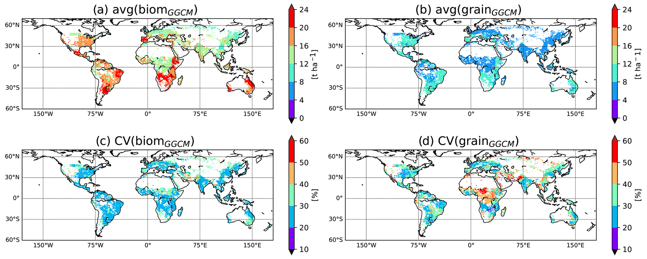
Figure 1 GGCM divergence in simulation of potential aboveground biomass and yield. Average and coefficient of variation for both aboveground biomass (biom) and yield (grain) computed among eight GGCMs used in the current analysis for simulations approaching potential yield in GGCMI (i.e., harmnon×irrigated for LPJ-GUESS, LPJmL, CLM-crop, pDSSAT, pAPSIM, GEPIC, and EPIC-IIASA and default×irrigated for CGMS-WOFOST; see Sect. 2.2.1). Only grid cells common to the eight GGCMs are considered for this figure. For GEPIC and EPIC-IIASA, the variable biom has been corrected (see Sect. 2.2.1). For the comparison including GGCMs that provide biom and grain for harmnon×irrigated simulation in GGCMI but which are not part of the current paper (i.e., EPIC-BOKU, PEPIC, and PEGASUS), see Fig. S1 in the Supplement.

2 Methods

2.1 GGCM emulator

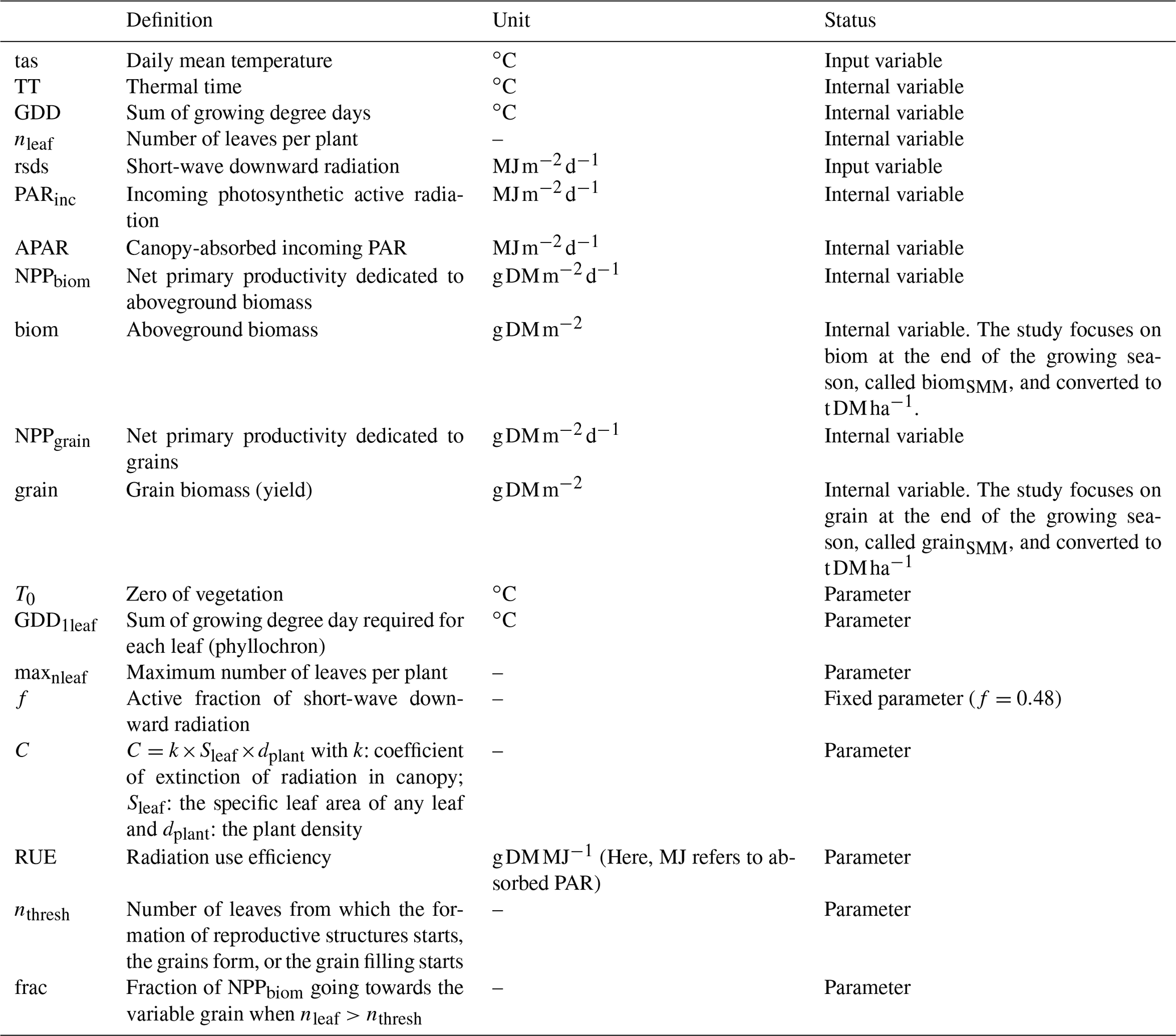
For any given day d of the growing season (defined here as the period between the planting day, t_p, and the crop maturity, t_m), we used the Eqs. (1)–(7), which rely on concepts commonly used in modeling of ecosystem productivity to compute the potential aboveground biomass (biom, in t DM ha⁻¹, with 1 ha = 0.01 km²). Variables and parameters are summarized in Table 1, and a simplified flow chart is given in Fig. S3 in the Supplement.

Table 1 List of variables and parameters in SMM.

For any d in [t_p, t_m], the thermal time (TT) is computed from the daily mean temperature (tas, in ^∘C) by using a reference temperature (T₀):

$$\begin{array}{}\text{(1)}& \text{TT}\left(d\right)=\text{tas}\left(d\right)-T_{\mathrm{0}}.\end{array}$$

GDD is the sum of growing degree days, defined as follows:

$$\begin{array}{}\text{(2)}& \text{GDD}\left(d\right)={\sum }_{i\le d}max\left(\mathrm{0},TT\left(i\right)\right).\end{array}$$

The number of leaves per plant (n_leaf) is computed from GDD and one parameter representing the thermal requirement for the emergence of any leaf (GDD_1leaf):

$$\begin{array}{}\text{(3)}& n_{\text{leaf}}\left(d\right)=min\left({\text{max}}_{\text{nleaf}},\text{GDD}\left(d\right)/{\text{GDD}}_{\text{1leaf}}\right),\end{array}$$

where max_nleaf is the maximum number of leaves. In our model, as soon as one leaf emerges, we assumed that it reaches its fully expanded leaf area, which is the same for all leaves (individual leaf area, called S_leaf hereafter). The incoming photosynthetic active radiation (PAR_inc) is derived from the short-wave downwelling radiation (rsds in $\mathrm{MJ}{\mathrm{m}}^{-\mathrm{2}}{\mathrm{d}}^{-\mathrm{1}}$) and its active fraction, f:

$$\begin{array}{}\text{(4)}& {\text{PAR}}_{\text{inc}}\left(d\right)=f\times \text{rsds}\left(d\right).\end{array}$$

The absorbed PAR by the canopy (APAR) is determined by assuming an exponential function according to the Beer–Lambert law:

$$\begin{array}{}\text{(5)}& \text{APAR}\left(d\right)={\text{PAR}}_{\text{inc}}\left(d\right)\times \left(\mathrm{1}-\exp \left(-C\times n_{\text{leaf}}\left(d\right)\right)\right),\end{array}$$

where C is a constant (see below). The net primary productivity dedicated to the aboveground biomass (NPP_biom) is computed from APAR with a constant radiation use efficiency (RUE in g DM MJ⁻¹):

$$\begin{array}{}\text{(6)}& {\text{NPP}}_{\text{biom}}\left(d\right)=\text{RUE}\times \text{APAR}\left(d\right).\end{array}$$

The aboveground biomass corresponds to the sum over time of NPP_biom:

$$\begin{array}{}\text{(7)}& \text{biom}\left(d\right)={\sum }_{i\le d}\left({\text{NPP}}_{\text{biom}}\left(i\right)\right).\end{array}$$

The parameter C of Eq. (5) can be decomposed in different parameters:

$$\begin{array}{}\text{(8)}& C=k\times S_{\text{leaf}}\times d_{\text{plant}},\end{array}$$

where k is the light extinction coefficient, S_leaf is the individual leaf area, and d_plant is the plant density. The product of S_leaf, d_plant and the number of leaves of a given day d (i.e., n_leaf(d)), corresponds to the leaf area index (LAI) of the same day:

$$\begin{array}{}\text{(9)}& \text{LAI}\left(d\right)=S_{\text{leaf}}\times d_{\text{plant}}\times n_{\text{leaf}}\left(d\right),\end{array}$$

in such a way that Eq. (5) can be re-written as follows:

$$\text{APAR}\left(d\right)={\text{PAR}}_{\text{inc}}\left(d\right)\times \left(\mathrm{1}-\exp \left(-k\times \text{LAI}\left(d\right)\right)\right)\left(\mathrm{5}\text{bis}\right),$$

We preferred Eq. (5) over Eq. (5bis) as we cannot separately calibrate the different parameters composing C and because we do not have any information about the LAI from GGCMs (see Sect. 4).

To compute the grain biomass at maturity, we first define the day l as follows:

$$\begin{array}{}\text{(10)}& n_{\text{leaf}}\left(l\right)\ge n_{\text{thresh}},\end{array}$$

From day l, a fixed fraction (frac) of NPP_biom constitutes the net primary productivity dedicated to the variable grain (called NPP_grain):

$$\left\{\begin{array}{ll}\text{if}d\ge l,& {\text{NPP}}_{\text{grain}}\left(d\right)=\text{frac}\times {\text{NPP}}_{\text{biom}}\left(d\right),\left(\mathrm{11}\right)\\ \text{if}d<l,& {\text{NPP}}_{\text{grain}}\left(d\right)=\mathrm{0}.\left(\mathrm{12}\right)\end{array}\right.$$

and finally,

$$\begin{array}{}\text{(13)}& \text{grain}\left(d\right)={\sum }_{i\le d}\left({\text{NPP}}_{\text{grain}}\left(i\right)\right).\end{array}$$

The variable grain (in t DM ha⁻¹) could be considered either as reproductive structures+grains or grains only. The parameter n_thresh is a threshold in the number of leaves from which either the formation of reproductive structures starts, the grains form, or grain filling starts. The above equations aim to be generic and to reproduce the diversity of approaches in GGCMs. That is why we do not distinguish between the production of reproductive structures and the accumulation of assimilates in grains after anthesis.

Equations (1)–(7) and (10)–(13) are called SMM (for simple mechanistic model) in the following. We focused on biom and grain at maturity, i.e., computed on the last day of the growing season t_m. They are called biom_SMM and grain_SMM in the following:

$$\begin{array}{}\text{(14)}& {\displaystyle }& {\displaystyle }{\text{biom}}_{\text{SMM}}=\text{biom}\left(t_{\mathrm{m}}\right),\text{(15)}& {\displaystyle }& {\displaystyle }{\text{grain}}_{\text{SMM}}=\text{grain}\left(t_{\mathrm{m}}\right).\end{array}$$

The variable grain_SMM is used to approach the potential yield. Our analysis focuses on maize because of the importance of cereals in human food and because of the widespread distribution of this crop across latitudes.

2.2 Set-up

We focused first on the computation of biom_SMM and then on the relationship grain_SMM vs. biom_SMM. The sensitivity of SMM to each parameter involved in the computation of biom_SMM was first studied. Then, we calibrated SMM against each GGCM to make the spatial distribution of biom_SMM mimic the spatial distribution of aboveground biomass at maturity simulated by each GGCM (hereafter called biom_GGCM). This calibration happened in two steps. The first step concerned C and RUE, which have one value at the global scale. The second step concerned GDD_1leaf, which we made varying in space to mimic procedure used by GGCM modellers in GGCMI (see below). The choice of focusing on C, RUE, and GDD_1leaf is justified below. In the last step (step 3), we calibrated n_thresh and frac to make SMM mimic the relationship grain vs. biom of each GGCM.

2.2.1 GGCMs and GGCMI simulations considered

The eight GGCMs considered in our approach were LPJ-GUESS (Lindeskog et al., 2013; Smith et al., 2001), LPJmL (Bondeau et al., 2007; Waha et al., 2012), CLM-crop (Drewniak et al., 2013), pDSSAT (Elliott et al., 2014; Jones et al., 2003), pAPSIM (Elliott et al., 2014; Keating et al., 2003), CGMS-WOFOST (Boogaard et al., 2014), GEPIC (Williams et al., 1995; Folberth et al., 2012; Izaurralde et al., 2006; Liu et al., 2007), EPIC-IIASA (Williams et al., 1995; Izaurralde et al., 2006). GGCMs simulations are provided in the framework of the GGCM Intercomparison (GGCMI) and described in Müller et al. (2019). GGCMI is an activity of the of the Agricultural Model Intercomparison and Improvement Project (AgMIP; Rosenzweig et al., 2013) and is an element of a broader AgMIP effort to explore cropping system responses to climate conditions and climate changes to facilitate applications including toward integrated assessment (Ruane et al., 2017). Six other GGCMs also participated in GGCMI but were not considered here as necessary output variables (timing and duration of the growing season for EPIC-BOKU, PEPIC, EPIC-TAMU; aboveground biomass for ORCHIDEE-crop) or simulations (for PRYSBI2) were not provided on the data archive of GGCMI.

In GCCMI, all GGCMs followed a common protocol and were forced by the same weather datasets. We focused here on the simulations forced by one of them, the AgMERRA dataset (Ruane et al., 2015). We used simulations forced by the AgMERRA dataset as all GGCMs performed these simulations. Three levels of harmonization have been used in GGCM simulations: default, fullharm, harmnon. In fullharm simulations, all GGCMs have been forced by the same prescribed beginning and end of the growing season, which were derived from a combination of two global datasets (MIRCA, Portmann et al., 2010; and SAGE, Sacks et al., 2010; Elliott et al., 2015). In harmnon simulations, in addition to forced timing and duration of the growing season, all GGCMs experienced no nutrient limitation through prescribed fertilizer inputs. Besides this harmonization level, two water regimes have been considered: irrigated and non-irrigated. For our analysis focusing on the simulation of potential yield, we decided to select the configuration (harmnon and irrigated). This is true for all GGCMs considered except CGMS-WOFOST. In fact, the harmnon simulation was not provided for CGMS-WOFOST but because (i) this model does not consider nutrient limitation and (ii) the growing season was prescribed in the default simulation, we assumed that the potential yield could be approached by the (default and irrigated) simulation.

For EPIC family models (here, GEPIC and EPIC-IIASA), we used a corrected biom_GGCM computed as below, as it has been noticed that some issues related to the variable biom appeared in the outputs available on the GGCMI data archive that are likely related to the output time step of specific variables (Folberth, personal communication, 2019):

$$\begin{array}{}\text{(16)}& {\text{biom}}_{\text{GGCM}}={\text{grain}}_{\text{GGCM}}/{\text{HI}}_{\text{max}},\end{array}$$

where HI_max is the maximum harvest index (no unit), varying in space as a function of cultivars. In EPIC, the actual HI at harvest only differs to HI_max if a drought stress occurs in the reproductive phase. Because this stress was virtually eliminated by sufficient irrigation in the harmnon×irrigated simulations, Eq. (16) provides the most accurate estimate of aboveground biomass at harvest. Maps of cultivar distribution, used as input to the EPIC models (Fig. 1 and Table D in Folberth et al., 2019), have been considered here to compute the corrected biom_GGCM.

2.2.2 Input variables for SMM

We focused our analysis on the growing season starting in calendar year 2000 (and potentially finishing in calendar year 2001). SMM was forced by the short-wave downwelling radiation (rsds in $\mathrm{MJ}{\mathrm{m}}^{-\mathrm{2}}{\mathrm{d}}^{-\mathrm{1}}$) and the daily mean temperature (tas, in ^∘C) from the AgMERRA weather dataset (Ruane et al., 2015). SMM also needs the beginning and end of the maize growing season, and we used the planting day (t_p) and the timing of maturity (t_m), respectively, both being provided in the output of each GGCM. Despite the fact that all GGCMs are forced by the same growing season in harmnon, some GGCMs allow flexibility in regards to t_p and t_m prescribed as input (Müller et al., 2017), as suggested by the GGCMI protocol: “crop variety parameters (e.g., required growing degree days to reach maturity, vernalization requirements, photoperiodic sensitivity) should be adjusted as much as possible to roughly match reported maturity dates”. Thus, we cannot use t_p and t_m from GGCM input files (Text S1 in the Supplement).

We performed SMM simulations (and thus, computed biom_SMM and grain_SMM) for each GGCM, i.e., for each GGCM growing season. For a given GGCM, SMM simulations were performed only for grid cells considered in the given GGCM. In addition, grid cells for which information about the growing season from MIRCA and SAGE was not available are masked to prevent to consider grid cells where internal GGCM computation was performed.

The maps of cultivar distribution used by EPIC models (Folberth et al., 2019) were also used as inputs to SMM in the simulation aiming to mimic the biom vs. grain relationship of EPIC models (see Sect. 2.2.4).

2.2.3 Sensitivity of global biom_SMM to SMM parameters

Except the active fraction of short-wave downward radiation (f in Eq. 4) the value of which is physically well-known, other parameters involved in the computation of biom_SMM (T₀, max_nleaf, GDD_1leaf, C, RUE) are relatively uncertain. The sensitivity of the global averaged biom_SMM to these parameters was assessed by performing 3125 (i.e., 5⁵) SMM simulations, allowing for the combination of five different values for each parameter. In each of these SMM simulations, a given parameter was constant in space. The initial estimate of each parameter was provided in Table S1. While the initial estimate of each parameter was based on the literature, we chose quite arbitrarily the same range of variation of [50 %–150 %] (in % of the initial estimate) for all parameters, with the five values tested uniformly distributed within the range of variation (i.e., 50 %, 75 %, 100 %, 125 %, 150 % of initial guess).

Following our current knowledge based on observations, it would be partly possible to choose a different uncertainty range for each parameter: for instance, the literature tends to show that RUE is relatively well constrained for maize (Sinclair and Muchow, 1999), while the C parameter, which depends on plant density, is expected to vary a lot as a function of the farming practices (Sangoi et al., 2002; Testa et al., 2016) (Table S1). However, SMM aimed to mimic GGCMs and not observations, and it is quite difficult to know if parameter values used in GGCMs reflect our current knowledge well. For instance, there is some confusion in values of RUE reported in the literature following the diversity of experimental approaches and units of expression that have been used (Sinclair and Muchow, 1999). Some confusion in RUE values exists in the literature between RUE expressed in g DM MJ⁻¹ of intercepted solar radiation (called here RUE^′) or in g DM MJ⁻¹ of intercepted PAR (RUE^′′, with ${\text{RUE}}^{\prime \prime }={\text{RUE}}^{\prime }/\mathrm{0.5}$) or in g DM MJ⁻¹ of absorbed PAR (RUE^′′′, with ${\text{RUE}}^{\prime \prime \prime }={\text{RUE}}^{\prime }/\mathrm{0.425}$) (Sinclair and Muchow, 1999), and this could lead to erroneous values in GGCMs. In the following we used MJ of absorbed PAR to be consistent with our Eq. (6). Observations also showed that RUE decreases during grain filling following the mobilization of leaf nitrogen to the grain (Sinclair and Muchow, 1999). Thus, RUE is larger during vegetative growth (3.8–4.0 g DM (MJofabsorbedPAR)⁻¹; Kiniry et al., 1989) than averaged over the whole season (3.1–4.0 g DM MJ⁻¹; Sinclair and Muchow, 1999). It is likely that some GGCMs used RUE values which are not representative to the whole growing season. Thus, we used the same range of uncertainty for all parameters in our calibration procedure. Exploring a wider range of values also allows for a more complete assessment of GGCM performance.

Potential confusion in units mentioned above also led us to choose an initial estimate of RUE (2 g DM MJ⁻¹) lower than values commonly reported in the literature (3.1–4.0 g DM MJ⁻¹) (Sinclair and Muchow, 1999); however, note that the highest values of RUE tested during our calibration (3.0 g DM MJ⁻¹) reach the literature-based range.

The global mismatch between each GGCM and SMM was quantified thanks to the root-mean-square error (RMSE), computed as follows:

$$\begin{array}{ll}\text{(17)}& {\displaystyle }& {\displaystyle }\text{RMSE}\left(u\right){\displaystyle }& {\displaystyle }=\sqrt{{\displaystyle \frac{\mathrm{1}}{N}}{\sum }_{g=\mathrm{1}}^N{\left({\text{biom}}_{\text{SMM}}\left(u,g\right)-{\text{biom}}_{\text{GGCM}}\left(g\right)\right)}^{\mathrm{2}}},\end{array}$$

where u is a combination of parameters and g is a grid cell among the N grid cells considered for each GGCM. All grid cells are assumed independent and have the same weight in the RMSE computation. RMSE has the same unit as biom (t DM ha⁻¹).

2.2.4 SMM calibration against each GGCM

SMM was calibrated following three steps. The first two steps aimed to mimic biom_GGCM distribution, while the last step aimed to make SMM reproduce the relationship grain vs. biom of each GGCM. The procedure of calibration was summarized in Table 2. “Emulated GGCM” is used from now to define SMM output after SMM calibration, aiming to mimic a given GGCM.

Table 2 Strategy of SMM calibration for each parameter.

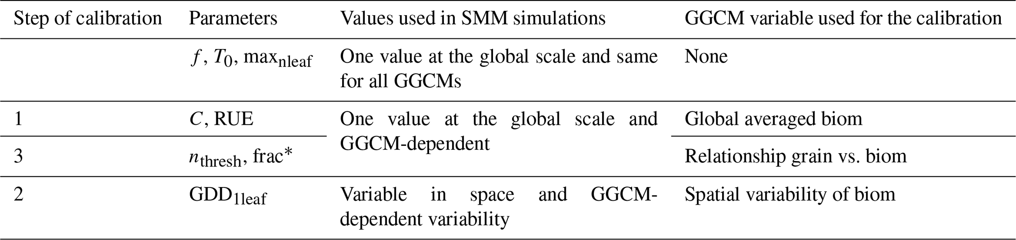
^* n_thresh and frac are variable in space as a function of the cultivar when SMM aims to mimic EPIC family models as these latter consider some cultivar diversity in harvest index.

Parameters involved in the computation of biom_SMM

Regarding the simulation of biom, we restricted the calibration to RUE, C, and GDD_1leaf as follows: f is well constrained, max_nleaf has a small effect on global simulated biom_SMM (see the results of the analysis prescribed in Sect. 2.2.3), and T₀ co-varies with GDD_1leaf, and we decided to focus on GDD_1leaf (see below). These parameters (f, max_nleaf, T₀) were prescribed equal to their initial estimate and were the same for all SMM simulations.

We choose to make C and RUE globally constant and GGCM-dependent. The decision to not make C and RUE vary in space is consistent with the rule of parsimony, which we used to build SMM. It also follows the procedure commonly used in GGCMs that involved a similar approach. For instance, GEPIC is based on a biomass-energy conversion coefficient that does not vary in space (Folberth et al., 2016). Plant density (hidden in C) is constant in space in LPJmL (Schaphoff et al., 2018a). We calibrated C and RUE at the same time to assess potential compensation between these parameters in SMM. The three pairs (C, RUE) that minimized the global RMSE computed following Eq. (17) the most among the pairs tested were chosen. A fourth pair corresponding to (C, RUE), where C is equal to its initial estimate, has been used. The use of four different pairs aimed to assess the sensitivity of our conclusions to the parameter values. For each (C, RUE) pair, we finally calibrated GDD_1leaf. We made GDD_1leaf vary in space as it is allowed in the GGCMI exercise. In the GGCMI protocol, accumulated thermal requirements were adjusted to catch the growing season (duration and timing) prescribed as input in the harmnon GGCM simulation. In SMM, the procedure slightly differs as we calibrated thermal requirements to match biom_GGCM: for each grid cell, GDD_1leaf is chosen among its five possible values to minimize the absolute difference between biom_GGCM and biom_SMM. Grid cells were considered independently.

The ability of SMM to match the spatial distribution of biom_GGCM for each GGCM after SMM calibration was measured through the bias, RMSE, and Nash–Sutcliffe model efficiency coefficient (NS), defined as follows:

$$\begin{array}{}\text{(18)}& \text{NS}=\mathrm{1}-{\displaystyle \frac{{\sum }_{g=\mathrm{1}}^N{\left({\text{biom}}_{\text{SMM}}\left(g\right)-{\text{biom}}_{\text{GGCM}}\left(g\right)\right)}^{\mathrm{2}}}{{\sum }_{g=\mathrm{1}}^N{\left({\text{biom}}_{\text{GGCM}}\left(g\right)-\stackrel{\mathrm{‾}}{{\text{biom}}_{\text{GGCM}}}\right)}^{\mathrm{2}}}},\end{array}$$

where g refers to any grid cell and biom_GGCM is the average of biom_GGCM over grid cells. NS=1 means that SMM perfectly matches the spatial distribution of biom_GGCM.

To assess the mismatch between biom_GGCM and biom_SMM after SMM calibration for a given GGCM, we aimed to assess how a variable related to climate or soil type can contribute to this mismatch. To do so, we separated all grid cells within two sub-groups according to the value of this variable (e.g., one sub-group corresponding to grid cells with high temperatures and one sub-group with low temperatures) and assess if the RMSE is different for the two sub-groups. If yes, it would suggest that a process related to this variable (e.g., heat stress) could be missing in SMM.

Parameters involved in the computation of grain_SMM

C, RUE, and GDD_1leaf determine biom simulated by SMM at each time step. Two SMM parameters are involved in the computation of grain for any day from biom, namely n_thresh and frac. The calibration of these parameters aims to make SMM able to mimic the relationship between grain and biom at the end of the growing season from each GGCM. One global and GGCM-dependent pair (n_thresh, frac) was chosen by using the following criteria:

$$\left\{\begin{array}{l}\text{if}{A}_{\text{GGCM}}=\mathrm{0},\text{find}u\text{that minimizes}\left(\mathrm{19}\right)\\ R_{\text{slope}}\left(u\right)=\left|a_{\text{GGCM}}-a_{\text{SMM}}\left(u\right)\right|,\\ \text{if}{A}_{\text{GGCM}}\ne \mathrm{0},\text{find}u\text{that maximizes}\left(\mathrm{20}\right)\\ R_{\text{areas}}\left(u\right)=\left(\frac{A_{\text{GGCM}}\cap A_{\text{SMM}}\left(u\right)}{max\left(A_{\text{GGCM}},A_{\text{SMM}}\left(u\right)\right)}\right),\end{array}\right.$$

where u corresponds to a given pair (n_thresh, frac), A_X is the area defined by the grid cell clouds in the grain vs. biom space for X, and a_X is the slope of the linear regression grain_X∼biom_X, with X in {GGCM,SMM}.

In other words, if grain_GGCM vs. biom_GGCM is a line, (n_thresh, frac) is chosen to make the relationship between grain_SMM vs. biom_SMM linear with the same slope as the one of the GGCM. If grain_GGCM vs. biom_GGCM is not a line, the grid cells in the space grain_GGCM vs. biom_GGCM define a non-null area, called A_GGCM, and (n_thresh, frac) is chosen to make A_SMM as similar as possible to A_GGCM. EPIC family GGCMs introduced a cultivar diversity in parameters related to grain filling and, in that case, the calibration of (n_thresh, frac), instead of being done at the global scale, was made for each cluster of grid cells corresponding to a given cultivar. The distribution of cultivars from EPIC was used as input of SMM in that case.

2.3 Contribution of different processes to yield in SMM

We computed ratios between some SMM internal variables to assess the global contribution of different processes represented in SMM to the achievement of grain_SMM. The following ratios have been computed: $n_{\text{leaf}}/\text{tas}$, $\text{APAR}/\text{rsds}$, $\text{APAR}/n_{\text{leaf}}$, $\text{biom}/\text{APAR}$, and $\text{grain}/\text{biom}$. The ratio $n_{\text{leaf}}/\text{tas}$ represents the phenology sensitivity to temperature, $\text{APAR}/\text{rsds}$ reflects how radiation is absorbed by the canopy, $\text{APAR}/n_{\text{leaf}}$ represents the absorption sensitivity to phenology, $\text{biom}/\text{APAR}$ reflects the conversion from absorbed radiation to biomass, and $\text{grain}/\text{biom}$ represents the harvest index.

We also investigated how the contribution of the different processes to the achievement of grain_SMM varies between emulated GGCMs. Variations in these ratios reflects the difference in global averaged key parameters between emulated GGCMs. For instance, variations in $\text{grain}/\text{biom}$ between emulated GGCMs reflects differences in calibrated n_thresh and frac (Fig. S3).

To compute the different ratios, averages over the growing season were used for tas, rsds, APAR, and n_leaf, while the end of the growing season was used for biom and grain (so-called biom_SMM and grain_SMM, Eqs. 14 and 15). A given ratio was computed for each grid cell, and its grid-cell distribution was plotted in the following as a bar plot (Sect. 3.4 and Fig. 8).

3 Results

3.1 Global averaged biom_SMM: sensitivity to each parameter and calibration of (C, RUE)

As expected when looking at Eqs. (6) and (7), the global averaged biom_SMM sensitivity to RUE was large (Fig. 2). Varying RUE was the only way possible to capture the global averaged biom_GGCM for LPJ-GUESS (Fig. 2). The global averaged biom_SMM was only slightly sensitive to other parameters as compared to the sensitivity to RUE. When all parameters are equal to their initial estimate, RUE minimizing the RMSE computed following Eq. (17) was 1.0 (LPJ-GUESS), 2.0 (LPJmL), 1.5 (CLM-crop), 2.5 (pDSSAT), 1.5 (pAPSIM), 2.0 (CGMS-WOFOST), 1.5 (GEPIC), and 1.5 g DM MJ⁻¹ (EPIC-IIASA).

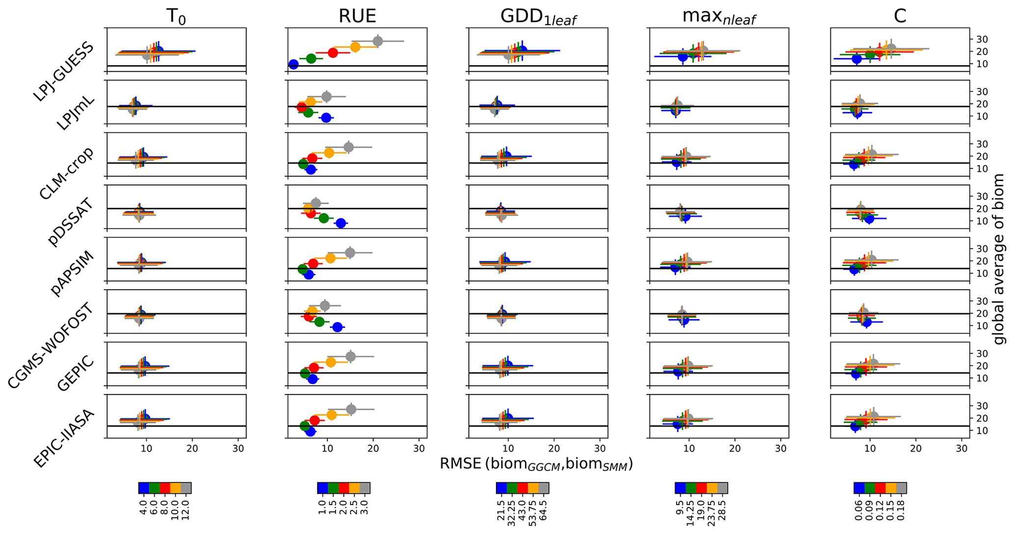
Figure 2 Global RMSE (biom_SMM, biom_GGCM) and global averaged biom_SMM sensitivity to SMM parameters. Five different values are used for each SMM parameter, and thus 5⁵ SMM simulations have been performed. The different lines correspond to the different GGCMs. For a given line and for a given column (i.e., for a given SMM parameter), each dot represents all SMM simulations sharing the same value for this parameter, which defines its color. Error bars correspond to the standard deviation among these SMM simulations. Each dot is defined through the RMSE(biom_GGCM,biom_SMM) (x axis, in t ha⁻¹) and the global averaged biom_SMM (y axis, in t ha⁻¹). The black horizontal line reports the global averaged biom_GGCM on the y axis. The difference of biom_SMM between rows for a given column results from differences in growth periods between GGCMs (and to a lesser extent from the difference in the spatial coverage of maize between GGCMs). Global values (average, RMSE) are computed by giving the same weight to each grid cell.

In Fig. 3, we plotted how RMSE changes according to both C and RUE varying at the same time, with all other parameters being equal to their initial estimate. Figure 3 shows that C and RUE can compensate in SMM. Calibrating (C, RUE) (with one global value for each parameter) allows the value to reach RMSE around 4 t DM ha⁻¹ for all GGCMs except LPJ-GUESS and LPJmL (around 2 and 3 t DM ha⁻¹ respectively) (Fig. 3). We chose 3 pairs (C, RUE) among the 25 tested couples that minimized the RMSE to assess the sensitivity of our conclusions to the pair chosen. Using a fourth pair with the same C for all GGCMs equal to its initial estimate decreased the ability of SMM to match the GGCMs only slightly (magenta dots in Fig. 3) and did not drastically change the RUE compared to the pairs where both C and RUE were calibrated.

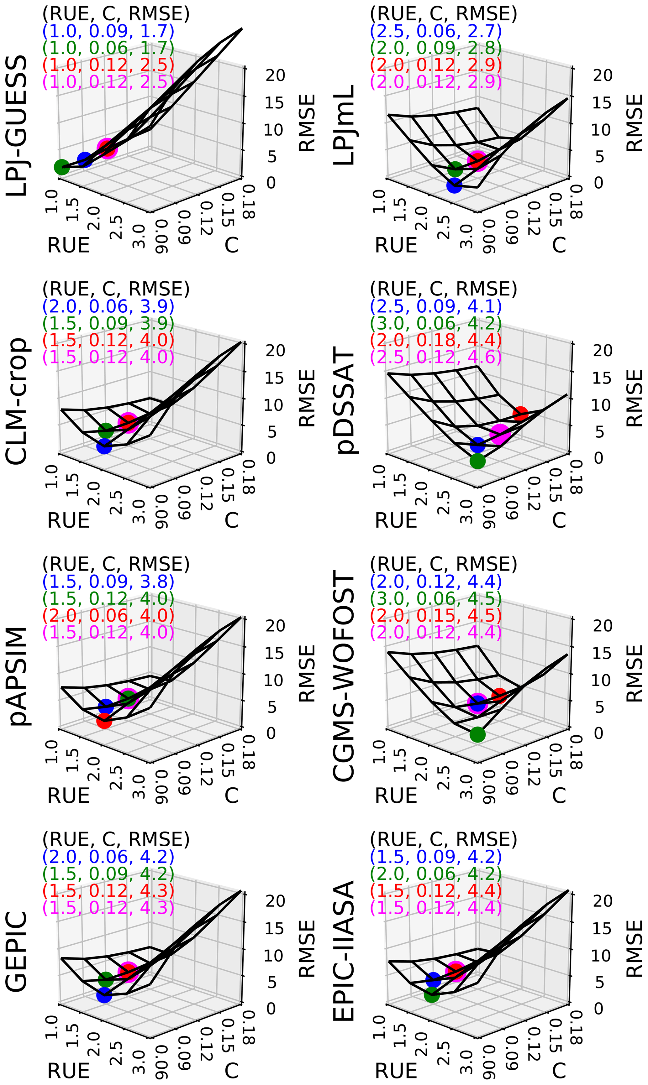
Figure 3 Sensitivity of global RMSE (biom_SMM, biom_GGCM) (t DM ha⁻¹) to C (−) and RUE (g DM MJ⁻¹) for each GGCM. For each GGCM, the shape of RMSE is derived from 25 SMM simulations (five values of C combined with five values of RUE). Other SMM parameters are equal to their respective initial estimate. For each GGCM, three (C, RUE) pairs that minimize the most RMSE among the 25 pairs tested are plotted in blue, green, and red. A fourth (C, RUE) pair minimizing the RMSE but with C equal to its initial estimate is shown in magenta. The values of the four (C, RUE) pairs and the corresponding RMSE are given in top left of each panel.

3.2 Calibration of GDD_1leaf

Once (C, RUE) was globally chosen, a spatially varying GDD_1leaf was calibrated. After calibration, SMM was able to catch the spatial variability of biom_GGCM for most GGCMs (Figs. 4 and 5a). Difference in percent can be large, especially for regions with small biom, but the global distribution was relatively well captured (Fig. 4).

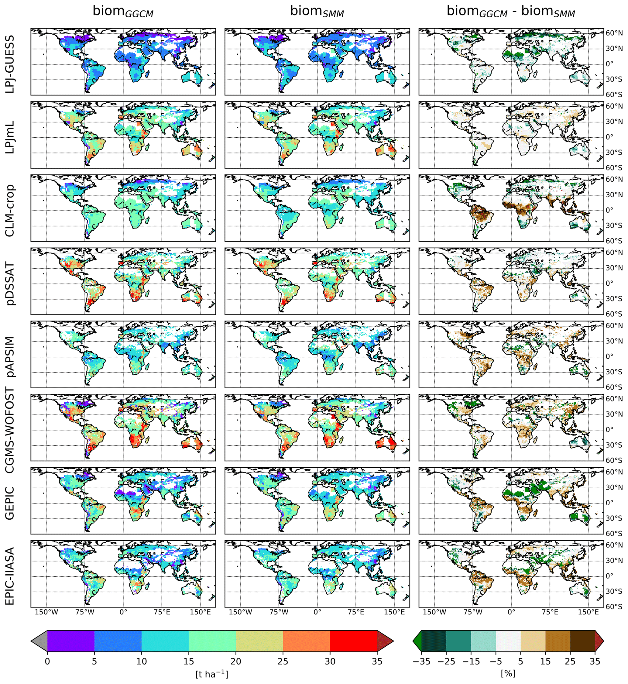
Figure 4 Comparison of the spatial distribution of simulated aboveground biomass (biom) between GGCM and SMM after its calibration. For each GGCM (row), the following variables are displayed: biom_GGCM (left column), biom_SMM after SMM calibration (i.e., calibration of global GGCM-dependent C and RUE and spatially varying GDD_1leaf), and the difference between the two (biom_GGCM−biom_SMM) (expressed in percent of biom_GGCM). Only biom_SMM after SMM calibration with the first (C, RUE) pair is shown.

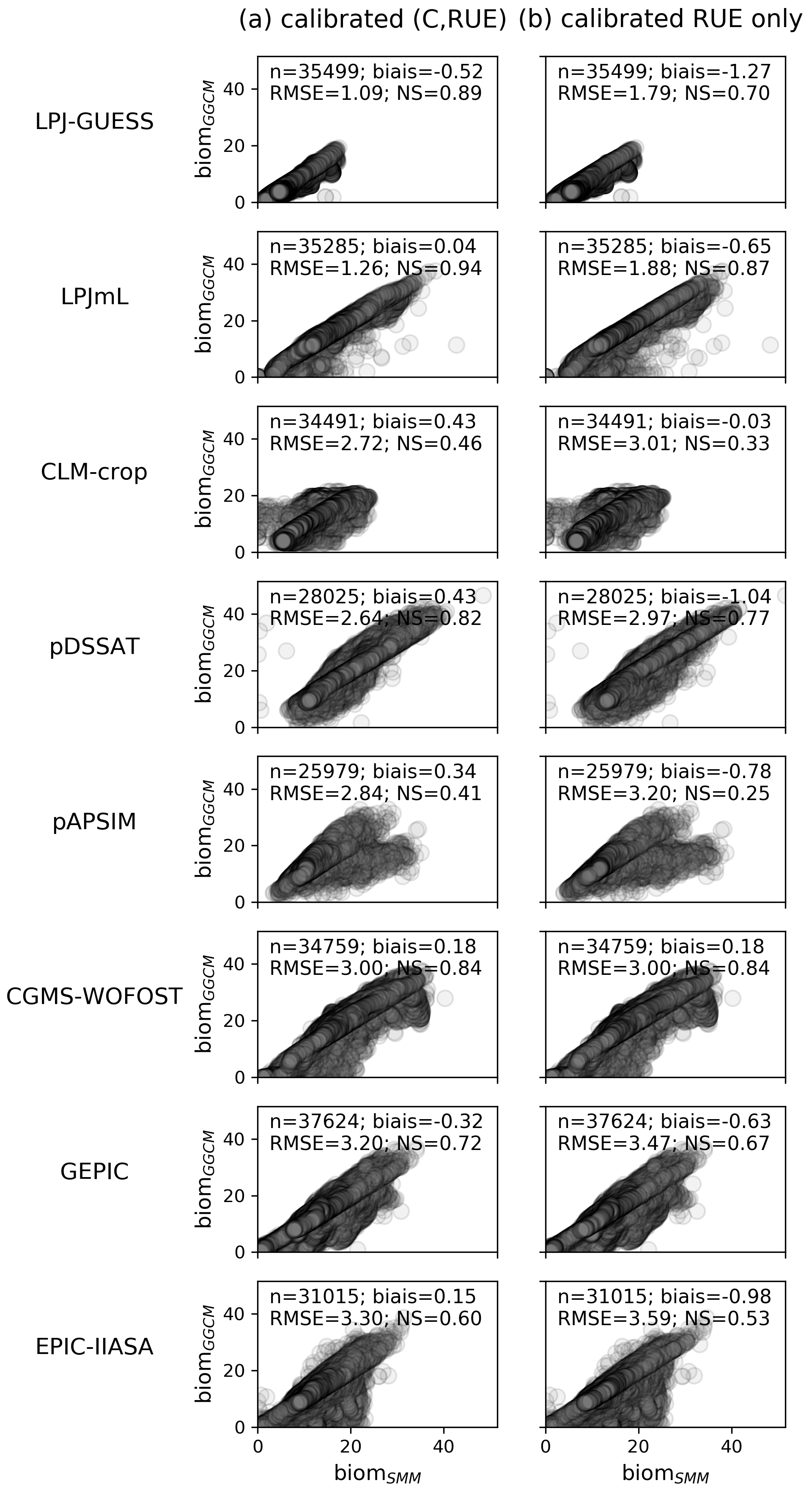
Figure 5 Scatterplots of biom_GGCM (y axis) vs. biom_SMM (x axis) after SMM calibration, i.e., calibration of global GGCM-dependent (C, RUE) and spatially varying GDD_1leaf. In (a) the (C, RUE) pair that minimizes the most the RMSE is used, while in (b) the (C, RUE) minimizing the RMSE with C equal to its initial estimate (the so-called fourth pair in Sect. 2.2.4) is used. Each dot corresponds to one grid cell. In the top left of each panel, the number of grid cells considered (n) and the different quantifications of the SMM vs. GGCM agreement (bias, RMSE, and NS) are given. See Fig. S6 in the Supplement for scatterplots of the four (C, RUE) pairs.

Global RMSE reaches between ∼1 (LPJ-GUESS) and 3.3 t DM ha⁻¹ (EPIC-IIASA) (Fig. 5a). The Nash–Sutcliffe coefficient (NS) is large (≥0.6) for all GGCMs but CLM-crop (0.46) and pAPSIM (0.41). RMSE is greater if computed for grid cells that experience some days with temperature above 30 ^∘C than if computed for grid cells without such days, i.e., for LPJ-GUESS (1.5 t DM ha⁻¹ vs. 0.8), GEPIC (4.4 vs. 2.3), EPIC-IIASA (4.2 vs. 2.8), and pAPSIM (3.5 vs. 2.3) (not shown). Nevertheless, the implementation of a heat stress within SMM (Text S2 in the Supplement) only slightly increases the fit of SMM vs. GGCM for these GGCMs: for example, NS increases from 0.41 (without heat stress) to 0.52 (with heat stress) for pAPSIM (Fig. S5 in the Supplement). The limited increase can be explained by the fact that optimized GDD_1leaf in the SMM simulation without heat stress encompasses a part of the heat stress for these grid cells.

EPIC family GGCMs simulate some other stresses, such as stresses related to salinity and aeration, that could have an effect on the potential yield even in the (harmnon and irrigated) simulations (Müller et al., 2019). The intensity of some of these stresses (aeration) depends on soil orders and should be particularly important in Vertisols (Christian Folberth, personal communication, 2019). However, RMSE is only slightly different for grid cells characterized by Vertisols vs. others soil orders for GEPIC (3.4 for Vertisols vs. 3.2 for other soil orders) and EPIC-IIASA (3.8 vs. 3.3).

CLM-crop (NS=0.46) and pAPSIM (NS=0.52 for SMM configuration with heat stress) are the two GGCMs for which the GGCM vs. SMM agreement remains relatively poor.

When using other (C, RUE) pairs, the fit SMM vs. GGCM overall slightly decreases for most GGCMs as the (C, RUE) chosen tends to lower global fit when GDD_1leaf is constant (see RMSE for the different pairs given in Fig. 3) but the same conclusions as above are reached: the fits are relatively correct, except for CLM-crop and pAPSIM (Fig. S6). Calibrating GDD_1leaf when the fourth (C, RUE) pair is used leads to reasonable fit between SMM and GGCM (Fig. 5b): calibrating C is of the second-order importance compared to the calibration of RUE.

The distribution of calibrated GDD_1leaf is provided in Fig. 6. This distribution varies between GGCMs. Most of the grid cells are characterized by extreme GDD_1leaf values. The distribution of GDD_1leaf is also sensitive to the chosen (C, RUE) pair, particularly for LPJ-GUESS and LPJmL. For these GGCMs, the difference (biom_GGCM−biom_SMM) is small and has the same sign almost everywhere (Fig. 4, last column). The sign is sensitive to the chosen (C, RUE): for instance, the difference is negative for the first (C, RUE) pair and positive for the second one for LPJ-GUESS. The calibration of GDD_1leaf, as it happens after the calibration of (C, RUE), tends to compensate this systematic bias and varies between pairs.

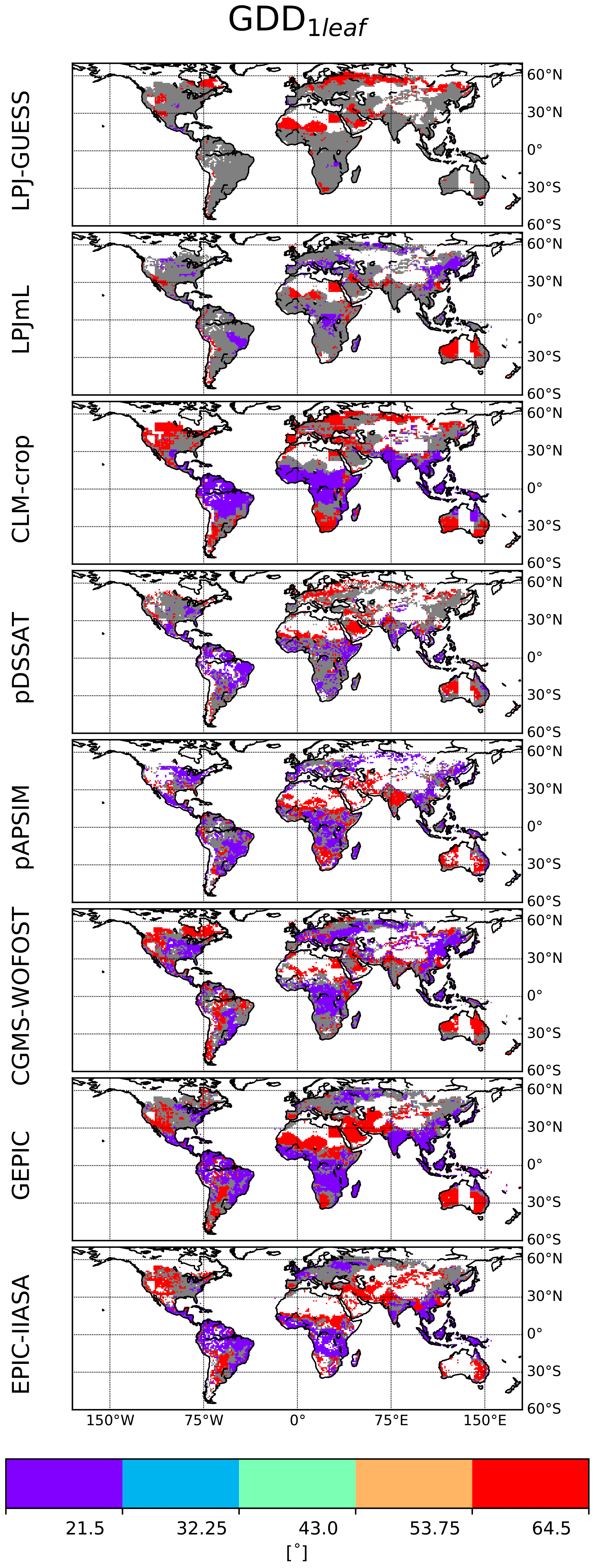
Figure 6 Calibrated spatial distribution of GDD_1leaf. Five values of GDD_1leaf are allowed (color scale and Table S1). Global GGCM-dependent (C, RUE) have been calibrated prior to GDD_1leaf and for a given GGCM; grid cells for which calibrated GDD_1leaf is different for the four (C, RUE) pairs are in grey.

A SMM simulation where the range of variation allowed for GDD_1leaf during the step two of the calibration is increased (from [50 %–150 %] of the initial estimate in the default calibration to [25 %–200 %] of the initial estimate) allows us to significantly improve the match between GGCM and SMM; the NS increases for CLM-CROP (from 0.46 to 0.66) and pAPSIM (from 0.41 to 0.60) (second column of Fig. S7 in the Supplement). Increasing the sensitivity to temperature by letting both GDD_1leaf and T₀ vary at the same time during the calibration gives similar results (third column of Fig. S7). These results are obvious, as allowing more variation in SMM allows a best fit to GGCM in more grid cells. This underlines the difficulty of making an SMM that functions as a mechanistic model (see Sect. 4).

3.3 Calibration of parameters involved in grain computation (n_thresh, frac)

Varying (n_thresh, frac) allows the dots (corresponding to the different grid cells) to define different shapes in the space yield_SMM vs. biom_SMM (e.g., Fig. S8 in the Supplement for pDSSAT). n_thresh=0 leads to a linear relationship between yield_SMM and biom_SMM with a slope equal to frac (left panels of Fig. S8). Non-null n_thresh make some grid cells deviate to this linear relationship and the number of such grid cells increases with n_thresh (Fig. S8). For all GGCMs, we found a (n_thresh, frac) combination that allows the relationship yield_SMM vs. biom_SMM to fit the relationship yield_GGCM vs. biom_GGCM (Fig. 7). For CLM-crop, we are not able to reproduce the cloud of dots corresponding to grid cells where the potential yield is below the line $\text{grain}=\mathrm{80}\mathit{\%}\times \text{biom}$. For EPIC family GGCMs, a calibration per cluster of grid cells sharing the same cultivar is required.

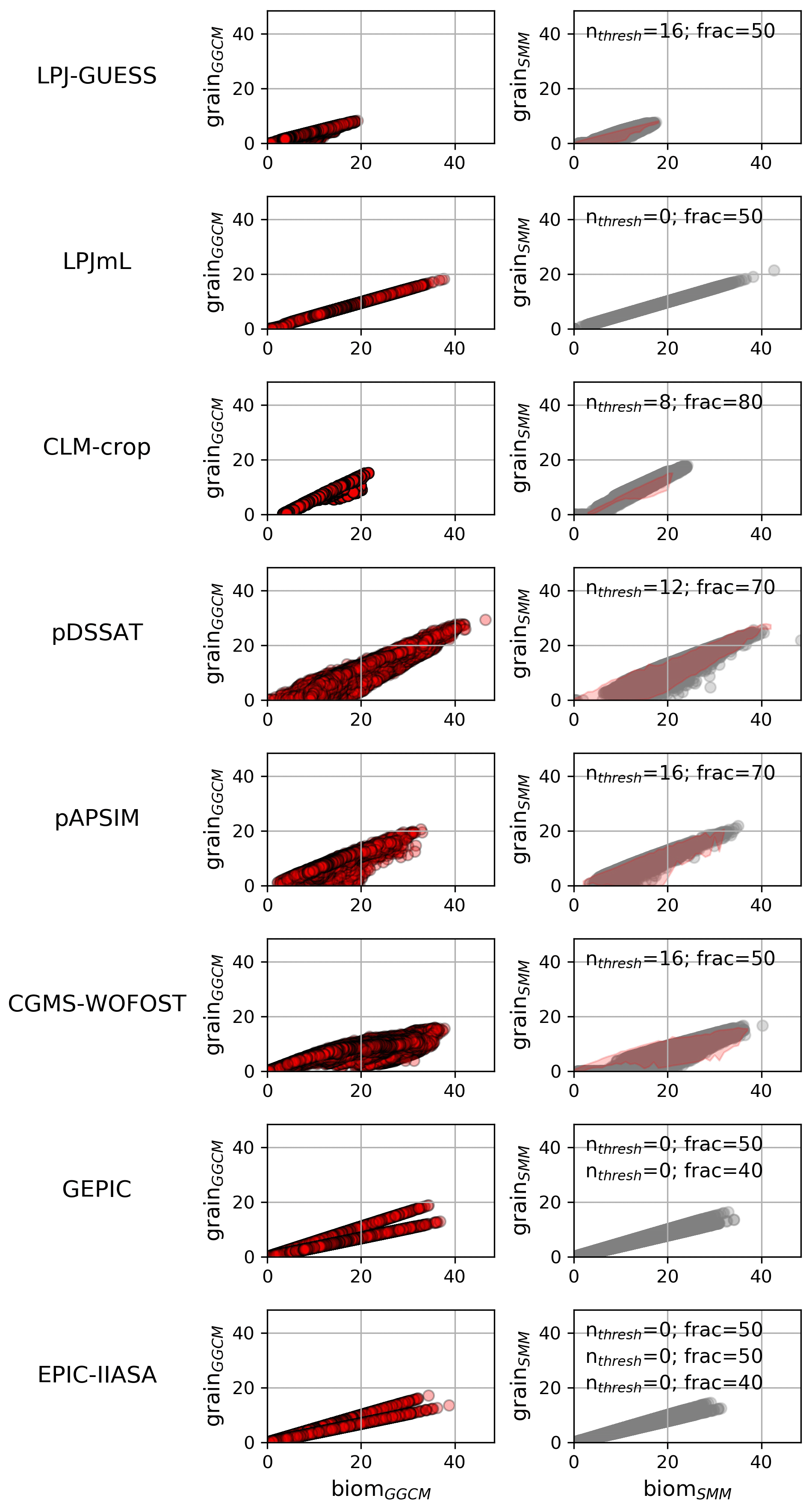
Figure 7 Relationship between grain and biom: comparison between GGCM and SMM after its calibration. The grain vs. biom relationship for GGCMs (left column) and for SMM after independent calibration against each GGCM (right column) are both displayed. For SMM, the relationship is given for the (n_thresh, frac) combination that maximizes the match between GGCM and SMM (see Sect. 2.2.4). The calibrated combination is given at the top of each SMM panel. When multiple cultivars are considered, one calibrated (n_thresh, frac) combination is given per cultivar. In the right-hand panels, pink shading defines A_GGCM (see Sect. 2.2.4).

3.4 Contribution of different processes to the achievement of grain_SMM

The ratio $n_{\text{leaf}}/\text{tas}$ is relatively constant among the emulated GGCMs, and this is true whatever the (C, RUE) pair is chosen (Fig. 8a). The ratio $n_{\text{leaf}}/\text{tas}$ reflects GDD_1leaf. The calibrated GDD_1leaf, even if its spatial distribution varies from one GGCM to the other (see Sect. 3.2), remains relatively constant at the global scale between GGCMs.

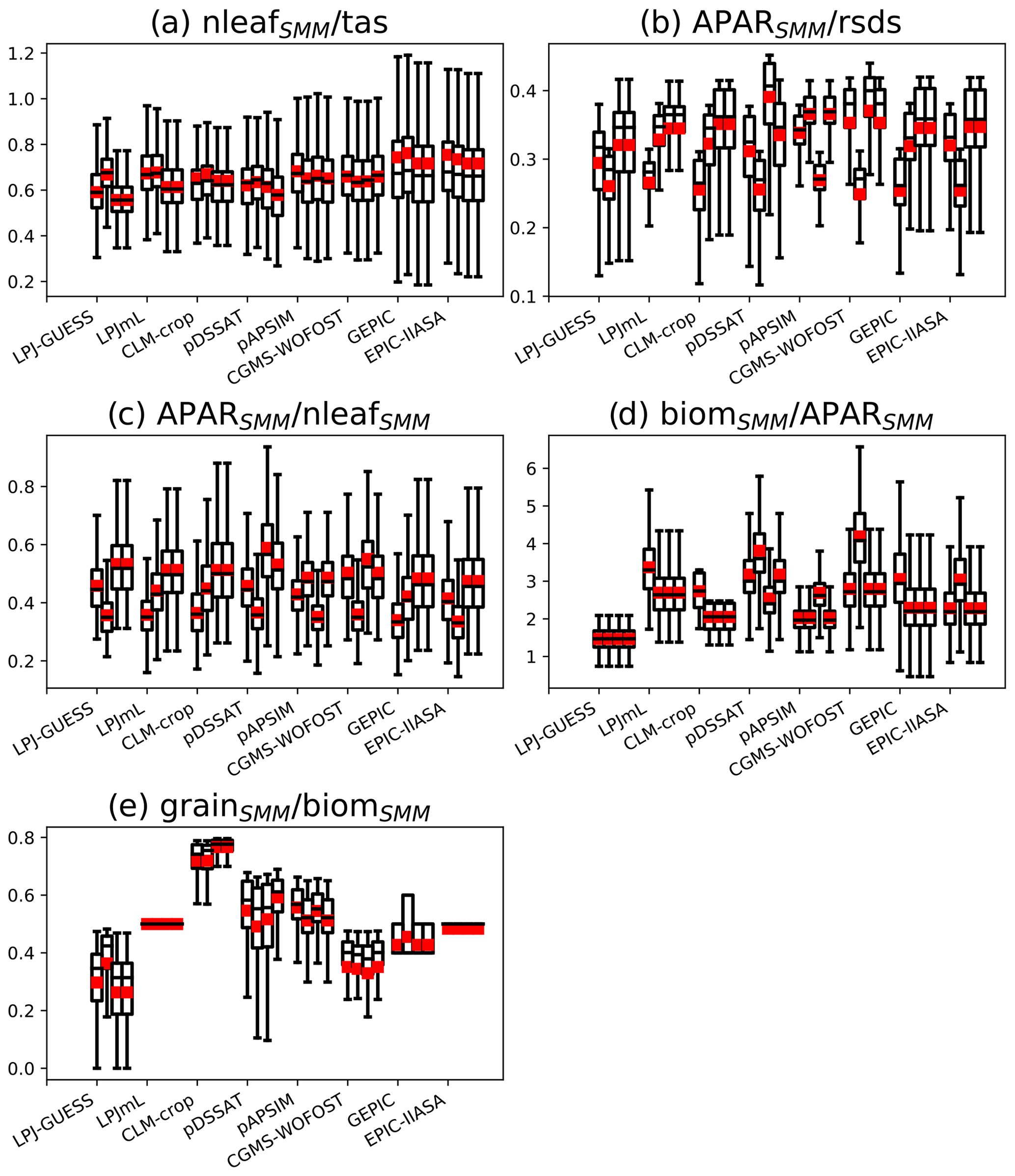
Figure 8 Bar plots of different ratios computed with SMM calibrated against each GGCM. Each panel shows a ratio (a $n_{\text{leaf}}/\text{tas}$, b $\text{APAR}/\text{rsds}$, c $\text{APAR}/n_{\text{leaf}}$, d $\text{biom}/\text{APAR}$, e $\text{grain}/\text{biom}$), while for a given panel x axis ticks correspond to emulated GGCMs. Four different (C, RUE) pairs have been tested and correspond to the four bars of each x axis tick.

The ratios $\text{APAR}/\text{rsds}$ and $\text{APAR}/n_{\text{leaf}}$ (Fig. 8b and c) vary a lot between GGCMs, but this variation is of the same order of magnitude as the one between (C, RUE) pairs. These ratios reflect C, which is highly variable between GGCMs and between pairs.

The ratio $\text{biom}/\text{APAR}$ (Fig. 8d) reflects global RUE. Calibrated RUE varies a lot between GGCMs and only slightly between pairs for a given GGCM.

The ratio $\text{grain}/\text{biom}$ (Fig. 8e) varies a lot between GGCMs and is only slightly sensitive to the (C, RUE) pair. This ratio reflects a combination of n_thresh and frac. GGCMs with n_thresh equal to 0 (LPJmL, EPIC-IIASA) have no grid cell variability in $\text{grain}/\text{biom}$ (Fig. 8e). Overall, regardless of the GGCM variability at grid cell scale, we can distinguish (i) emulated GGCMs that convert a large fraction of biom to grain, such as CLM-crop; (ii) emulated GGCMs that convert around 50 % of biom to grain, such as LPJmL, pDSSAT, GEPIC, pAPSIM, and EPIC-IIASA; and (iii) emulated GGCMs that convert around 30 %–40 % of biom to grain, such as LPJ-GUESS and CGMS-WOFOST. Large variation of $\text{grain}/\text{biom}$ between GGCMs is consistent with the fact that difference in grain among GGCMs is larger than the one in biom (Fig. 1).

4 Discussion and conclusions

We have shown that a simple set of equations with one GGCM-dependent global RUE and spatially variable thermal requirement (GDD_1leaf) is able to mimic spatial distribution of aboveground biomass of most GGCMs. Calibrating one additional global parameter at the same time as RUE (namely C) only slightly improves the fit between SMM and GGCM and only modified the calibrated value of RUE to a small extent. RUE represents canopy photosynthesis and GDD_1leaf determines crop duration, i.e., the two main drivers of crop productivity (Sinclair and Muchow, 1999). The relationship between potential yield and aboveground biomass of GGCM is captured by the calibration of two additional global parameters: one that triggers the start of grain filling and one corresponding to a time-invariant fraction of NPP allocated to the grain. These two parameters allow us to capture the relationship between biom and grain from all GGCMs. This feature of SMM is particularly important, as we have shown that the divergence between GGCMs is larger for grain than for biom (Fig. 1). Cultivar diversity regarding these latter parameters is nevertheless required to catch the behavior of some GGCMs. Despite the apparent complexity of GGCMs, we have shown that differences between them regarding potential yield can be explained by differences in a few key parameters.

Our approach has a few caveats. First, SMM could be able to fit individual GGCMs for the wrong reasons, i.e., following a compensation between SMM internal processes that is not representative of the considered GGCM. We think that this issue is nevertheless minimized in our approach. First, we investigated how parameters can compensate, e.g., by calibrating RUE and C at the same time. We showed that calibration of C is of second-order importance and that getting calibrated RUE to vary less among emulated GGCMs would require extreme values for C, well outside the range of values allowed in our calibration. The parameter C encompasses different parameters (see Eq. 8), and a better alternative would be to separate them as well as to explicitly simulate the leaf area index (LAI) variable. SMM-simulated LAI would be compared to GGCM output and this comparison would further reduce the risk of compensation between processes in SMM. However, LAI was neither available from GGCMI data archive nor upon request to GGCM modellers. We stress the need to incorporate this output variable in the next intercomparison exercise. It is also important to note that the average over the growing season of LAI or LAI at set fractions of the growing season (including anthesis) would be more interesting than LAI at harvest as, under potential conditions, LAI at harvest is very likely close to maximum LAI allowed by the different GGCMs.

Therefore, the reasonable match between SMM-simulated aboveground biomass and GGCM-simulated biom is made possible only because of the large range of variation allowed for RUE and GDD_1leaf during the calibration, i.e., [50 %–150 %] of their initial estimate. This range should have a meaning in term of values commonly used in GGCMs. Otherwise, the calibrated parameters could implicitly encompass different mechanisms considered in GGCMs but not in SMM, and this issue should become more likely as we choose a larger range of variations. For instance, calibrated GDD_1leaf in SMM could artificially encompass the sensitivity to temperature of processes not considered in SMM, as we discussed for heat stress in Sect. 3.2. It is likely that the variation of GDD_1leaf also encompasses a spatial variation of emergence in GGCMs, as in SMM we did not compute emergence and plants start to grow from the planting day. In such cases SMM should not be considered as a pure mechanistic model but more as a meta-model, and purely statistical meta-models should be more appropriate than our simplified process-based model. However, the range of variation that we used for GDD_1leaf ([50 %–150 %] around the initial estimate of 43 ^∘C, corresponding to $\sim \left[\mathrm{22}\text{–}\mathrm{65}{}^{\circ }\mathrm{C}\right]$) is consistent with ranges reported by observations focusing on the sensitivity of phyllochron (thermal requirement for the emergence of any leaf) to temperature (fig. 2 of Birch et al., 1998) and cultivar (Padilla and Otegui, 2005). Our range of GDD_1leaf cannot be straightforward compared to the range of heat units commonly used in GGCMs to catch the prescribed growing season (e.g., $\sim \left[\mathrm{10}\text{–}\mathrm{225}{}^{\circ }\mathrm{C}\right]$ in GEPIC if we divide the values of heat units given in Minoli et al., 2019, by a maximum number of leaves of 19, as in our study) or computed in van Bussel et al. (2019b) ($\sim \left[\mathrm{25}\text{–}\mathrm{160}{}^{\circ }\mathrm{C}\right]$ if we divide the values given in Fig. 2 of that latter reference by 19). Indeed, in our approach, GDD_1leaf×max_nleaf corresponds to the thermal requirement up to the emergence of all leaves, while the sum of heat unit used in GEPIC or van Bussel et al. (2015b) is required to reach plant maturity and thus encompasses both the emergence of all leaves and the period from flowering (concomitant to the end of leaf emergence) up to plant maturity.

Some discrepancies remain between SMM and some GGCMs, especially CLM-crop and pAPSIM. This could be explained by differences between GGCM and SMM in the choice of processes represented (e.g., net productivity in SMM instead of a balance between gross productivity and plant respiration in some GGCMs) or in the choice of equations used to represent a given process (e.g., Farquhar (CLM-crop) vs. RUE (SMM) for assimilation). The representation of stomatal conductance and CO₂ assimilation rate within Farquhar equations introduces a sensitivity to variables not considered in the RUE-based approach (e.g., water vapor pressure deficit), which is in line with observations that show that RUE is sensitive to many variables (Sinclair and Muchow, 1999). This would lead to differences in the spatial variability of simulated aboveground biomass as compared to one simulated with spatially constant RUE. The succession of phenological stages with different parameterizations in some GGCMs (e.g., in pAPSIM; Wang et al., 2002) can also partly contribute to differences with SMM because plant development is continuously simulated in SMM, as it is in other GGCMs (e.g., LPJmL, Schaphoff et al., 2018b). Another potential mismatch is related to some limiting factors (nutrients, water, etc.) that could exist in the harmnon and irrigated simulation for GGCMs (despite the protocol of these simulations) or through different biases. First, GGCMs that do not explicitly simulate nutrient limitations may have integrated these stresses implicitly in their parameterizations (discussed below). Second, irrigation in some GGCMs ensures that plants are not limited by water supply. However, plants can still experience water stress if the atmospheric demand is higher than the plant hydraulic structure can service. This could likely explain the lower yield for the group of grid cells below the line corresponding to ${\text{grain}}_{\text{GGCM}}=\mathrm{80}\mathit{\%}\times {\text{biom}}_{\text{GGCM}}$ for CLM-Crop in Fig. 7. Finally, some other stresses (salinity, aeration, etc.) are present in a few GGCMs (e.g., EPIC family models) and are not alleviated in harmnon simulation. However, it seems that these stresses, restricted to a few grid cells, cannot significantly contribute to the GGCM vs. SMM mismatch.

Despite some confusion in values of RUE reported in the literature arising from diversity of experimental approaches and units of expression that have been used (Sinclair and Muchow, 1999; Sect. 2.2.3), RUE is relatively well constrained from observations ([3.1–4.0] g DM MJ⁻¹). Here, we found that calibrated RUE values in emulated GGCMs are lower than values derived from observations and varied a lot among GGCMs: between 1 g DM MJ⁻¹ for LPJ-GUESS and 2.5 g DM MJ⁻¹ for pDSSAT. The values of calibrated RUE found in our study can be compared to values actually used in GGCMs based on the same approach of conversion of radiation to aboveground biomass. RUE used in GEPIC is equal to 4.0 g DM MJ⁻¹ (Christian Folberth, personal communication, 2020), while our calibrated value for the same GGCM is 2.0 g DM MJ⁻¹. Our calibrated RUE is an apparent RUE and the mismatch with actual RUE prescribed to GEPIC can be explained as follows. First, the daily increment of biomass in GEPIC derived from the conversion of radiation encompasses an increment for both aboveground biomass and roots (with a root : total ratio varying from 0.4 at germination to 0.2 at maturity), while both the RUE values used in SMM and derived from most observations (Sinclair and Muchow, 1999) concern aboveground biomass only. Actual RUE prescribed to GEPIC after correction to make it represent only aboveground biomass should vary between 2.4 at germination to 3.8 g DM MJ⁻¹ at maturity and is closer (particular in the first growth stages) to our calibrated RUE for GEPIC. Second, LAI_max in GEPIC is lower than values used in SMM: in GEPIC, LAI_max varies with plant density and is equal to 3.5 at plant density of 5 plants m⁻² used in the GGCMI simulations, while LAI_max in SMM is equal to 5 (this value can be derived from Eq. (9) when n_leaf reaches its maximum, i.e., max_nleaf, whose the value is prescribed during the calibration procedure; max_nleaf=19). Lower LAI_max in GEPIC than SMM can compensate for higher RUE. Some additional sensitivity tests with varying LAI_max (not shown) nevertheless suggest that the mismatch in LAI_max between GEPIC and SMM contributes only slightly to the mismatch in RUE. Finally, the seasonal dynamic of LAI could be different between GEPIC and SMM, and this can counterbalance the lower increment of biomass computed in SMM than in GEPIC once LAI_max is reached. As mentioned above, the values of LAI computed by GGCMs at different set fractions of the growing season would be very helpful.

The diversity in apparent RUE found between GGCMs raises a question about the physical meaning of the parameters used in each GGCM. GGCMs are tools that are primarily dedicated to simulating actual yield and could have been tuned for that purpose against local observations. During this tuning, processes not explicitly represented in a given GGCM could be implicitly incorporated into parameterizations of other processes. For instance, this could be the case for GGCMs that do not explicitly incorporate nutrient limitations. Potential yield is a variable that has been computed in a second step and that could suffer from these implicit incorporations. In the end, the divergence in potential yield between GGCMs raises questions about their ability to reproduce real processes as the basis of the actual yield, as this depends on the combination of potential yield and many limiting factors.

Our study has some implications for GGCM modellers in regards to the simulation of potential yield. We showed that differences between GGCMs can be explained by differences in a few key parameters, namely the RUE and parameters driving the grain filling (n_thresh and frac). For RUE, we recommend for GGCM modellers to investigate why each individual GGCM has a such a small (explicit or implicit) apparent RUE. We showed that n_thresh and frac vary a lot between GGCMs. For GGCMs with n_thresh equal to 0, a parametrization based on a better distinction between the emergence of all leaves and the period from flowering to maturity could be interesting. We also showed that n_thresh and frac determines harvest index (HI), and we showed that HI varies a lot between GGCMs. Thus, we advise that more effort needs to be directed toward assembling a global dataset of HI for either parametrization or evaluation of GGCMs. The maximum HI that a plant can reach is a cultivar characteristic, and one possibility to build such dataset could partly rely on information from seed companies. Finally, we suggested that the next intercomparison exercise encompass LAI and the beginning and end of the different growing season periods (vegetative period, flowering, etc.) for GGCMs that distinguish between such stages.

Model ensemble mean or median from an intercomparison exercise is commonly preferred to individual GGCM as it has better skill in reproducing the observations (Asseng et al., 2014; Martre et al., 2015). Our mechanistic model tuned against GGCMs could be a viable alternative to this ensemble mean and median as it allows us to keep track of processes leading to the final variable, namely the potential yield. Once tuned, SMM could be forced by an ensemble of parameters to reproduce the ensemble of GGCMs. Our emulator could also offer a potential for GGCM evaluation and analysis of their structural uncertainty. Its use under different climate and CO₂ conditions would nevertheless require the implementation of some missing mechanisms (e.g., heat stress and effect of CO₂).

For the purpose of simulating potential yield at the global scale, our emulator forced by daily temperature and radiation, growing season, and a few adjustable parameters could be considered an interesting alternative to GGCMs as they are easier to manipulate and allow much faster simulations. For instance, our model could be used to investigate the implementation of cultivar diversity at the global scale. The introduction of cultivar diversity is a keystone in development of crop models at the global scale (Boote et al., 2013). Cultivar diversity considered at the global scale was mainly related to phenological development through sensitivity to photoperiod and sensitivity to temperature (and vernalization for winter cultivars) (van Bussel et al., 2015a). The effect of cultivar diversity on allometry (e.g., through variability in harvest index) was considered in a less extensive extent at the global scale and restricted to some EPIC models (Folberth et al., 2019) or pDSSAT in a specific study (Gbegbelegbe et al., 2017). Through the protocol of GGCMI in which thermal requirements are tuned to match the growing season, cultivar diversity was implicitly accounted for. The same applies for SMM. The parameters of the emulator, here fitted to reproduce GGCM output, could also be fitted to global datasets based on census data and observations in a manner similar to that of PEGASUS (Deryng et al., 2011) but related to potential yield (against real yield for PEGASUS). For instance, SMM could be calibrated against the global dataset of potential yield based on statistical approach (Mueller et al., 2012), and the spatial variation of calibrated parameters could be compared to existing knowledge about the spatial distribution of cultivars. Finally, because it allows temporal dynamic simulation, our model could be coupled with simulation of limiting factors (water, nutrients) to investigate the limitation of potential yield at the global scale in a simple but mechanistic manner.