the Creative Commons Attribution 4.0 License.
the Creative Commons Attribution 4.0 License.
 | 17 Mar 2021
MLAir (v1.0) – a tool to enable fast and flexible machine learning on air data time series
Lukas Hubert Leufen
Felix Kleinert
Martin G. Schultz
With MLAir (Machine Learning on Air data) we created a software environment that simplifies and accelerates the exploration of new machine learning (ML) models, specifically shallow and deep neural networks, for the analysis and forecasting of meteorological and air quality time series. Thereby MLAir is not developed as an abstract workflow, but hand in hand with actual scientific questions. It thus addresses scientists with either a meteorological or an ML background. Due to their relative ease of use and spectacular results in other application areas, neural networks and other ML methods are also gaining enormous momentum in the weather and air quality research communities. Even though there are already many books and tutorials describing how to conduct an ML experiment, there are many stumbling blocks for a newcomer. In contrast, people familiar with ML concepts and technology often have difficulties understanding the nature of atmospheric data. With MLAir we have addressed a number of these pitfalls so that it becomes easier for scientists of both domains to rapidly start off their ML application. MLAir has been developed in such a way that it is easy to use and is designed from the very beginning as a stand-alone, fully functional experiment. Due to its flexible, modular code base, code modifications are easy and personal experiment schedules can be quickly derived. The package also includes a set of validation tools to facilitate the evaluation of ML results using standard meteorological statistics. MLAir can easily be ported onto different computing environments from desktop workstations to high-end supercomputers with or without graphics processing units (GPUs).
- Article
(2925 KB) - Full-text XML
- BibTeX
- EndNote


In times of rising awareness of air quality and climate issues, the investigation of air quality and weather phenomena is moving into focus. Trace substances such as ozone, nitrogen oxides, or particulate matter pose a serious health hazard to humans, animals, and nature (Cohen et al., 2005; Bentayeb et al., 2015; World Health Organization, 2013; Lefohn et al., 2018; Mills et al., 2018; US Environmental Protection Agency, 2020). Accordingly, the analysis and prediction of air quality are of great importance in order to be able to initiate appropriate countermeasures or issue warnings. The prediction of weather and air quality has been established operationally in many countries and has become a multi-million dollar industry, creating and selling specialized data products for many different target groups.
These days, forecasts of weather and air quality are generally made with the help of so-called Eulerian grid point models. This type of model, which solves physical and chemical equations, operates on grid structures. In fact, however, local observations of weather and air quality are strongly influenced by the immediate environment. Such local influences are quite difficult for atmospheric chemistry models to accurately simulate due to the limited grid resolution of these models and because of uncertainties in model parameterizations. Consequently, both global models and so-called small-scale models, whose grid resolution is still in the magnitude of about a kilometre and thus rather coarse in comparison to local-scale phenomena in the vicinity of a measurement site, show a high uncertainty of the results (see Vautard, 2012; Brunner et al., 2015). To enhance the model output, approaches focusing on the individual point measurements at weather and air quality monitoring stations through downscaling methods are applied allowing local effects to be taken into account. Unfortunately, these methods, being optimized for specific locations, cannot be generalized for other regions and need to be re-trained for each measurement site.
Recently, a variety of machine learning (ML) methods have been developed to complement the traditional downscaling techniques. Such methods (e.g. neural networks, random forest) are able to recognize and reproduce underlying and complex relationships in data sets. Driven in particular by computer vision and speech recognition, technologies like convolutional neural networks (CNNs; Lecun et al., 1998), or recurrent networks variations such as long short-term memory (LSTM; Hochreiter and Schmidhuber, 1997) or gated recurrent units (GRUs; Cho et al., 2014) but also more advanced concepts like variational autoencoders (VAEs; Kingma and Welling, 2014; Rezende et al., 2014), or generative adversarial networks (GANs; Goodfellow et al., 2014), are powerful and widely and successfully used. The application of such methods to weather and air quality data is rapidly gaining momentum.
Although the scientific areas of ML and atmospheric science have existed for many years, combining both disciplines is still a formidable challenge, because scientists from these areas do not speak the same language. Atmospheric scientists are used to building models on the basis of physical equations and empirical relationships from field experiments, and they evaluate their models with data. In contrast, data scientists use data to build their models on and evaluate them either with additional independent data or physical constraints. This elementary difference can lead to misinterpretation of study results so that, for example, the ability of the network to generalize is misjudged. Another problem of several published studies on ML approaches to weather forecasting is an incomplete reporting of ML parameters, hyperparameters, and data preparation steps that are key to comprehending and reproducing the work that was done. As shown by Musgrave et al. (2020) these issues are not limited to meteorological applications of ML only.
To further advance the application of ML in atmospheric science, easily accessible solutions to run and document ML experiments together with readily available and fully documented benchmark data sets are urgently needed (see Schultz et al., 2021). Such solutions need to be understandable by both communities and help both sides to prevent unconscious blunders. A well-designed workflow embedded in a meteorological and ML-related environment while accomplishing subject-specific requirements will bring forward the usage of ML in this specific research area.
In this paper, we present a new framework to enable fast and flexible Machine Learning on Air data time series (MLAir). Fast means that MLAir is distributed as full end-to-end framework and thereby simple to deploy. It also allows typical optimization techniques to be deployed in ML workflows and offers further technical features like the use of graphics processing units (GPUs) due to the underlying ML library. MLAir is suitable for ML beginners due to its simple usage but also offers high customization potential for advanced ML users. It can therefore be employed in real-world applications. For example, more complex model architectures can be easily integrated. ML experts who want to explore weather or air quality data will find MLAir helpful as it enforces certain standards of the meteorological community. For example, its data preparation step acknowledges the autocorrelation which is typically seen in meteorological time series, and its validation package reports well-established skill scores, i.e. improvement of the forecast compared to reference models such as persistence and climatology. From a software design perspective, MLAir has been developed according to state-of-the-art software development practices.
This article is structured as follows. Section 2 introduces MLAir by expounding the general design behind the MLAir workflow. We also share a few more general points about ML and what a typical workflow looks like. This is followed by Sect. 3 showing three application examples to allow the reader to get a general understanding of the tool. Furthermore, we show how the results of an experiment conducted by MLAir are structured and which statistical analysis is applied. Section 4 extends further into the configuration options of an experiment and details on customization. Section 5 delineates the limitations of MLAir and discusses for which applications the tool might not be suitable. Finally, Sect. 6 concludes with an overview and outlook on planned developments for the future.
At this point we would like to point out that in order to simplify the readability of the paper, highlighting is used. Frameworks are highlighted in italics and typewriter font is used for code elements such as class names or variables. Other expressions that, for example, describe a class but do not explicitly name it, are not highlighted at all in the text. Last but not least, we would like to mention that MLAir is an open-source project and contributions from all communities are welcome.
ML in general is the application of a learning algorithm to a data set whereby a statistical model describing relations within the data is generated. During the so-called training process, the model learns patterns in the data set with the aid of the learning algorithm. Afterwards, this model can be applied to new data. Since there is a large number of learning algorithms and also an arbitrarily large number of different ML architectures, it is generally not possible to determine in advance which approach will deliver the best results under which configuration. Therefore, the optimal setting must be found by trial and error.
ML experiments usually follow similar patterns. First, data must be obtained, cleaned if necessary, and finally put into a suitable format (preprocessing). Next, an ML model is selected and configured (model setup). Then the learning algorithm can optimize the model under the selected settings on the data. This optimization is an iterative procedure and each iteration is called an epoch (training). The accuracy of the model is then evaluated (validation). If the results are not satisfactory, the experiment is continued with modified settings (i.e. hyperparameters) or started again with a new model. For further details on ML, we refer to Bishop (2006) and Goodfellow et al. (2016) but would also like to point out that there is a large amount of further introductory literature and freely available blog entries and videos, and that the books mentioned here are only two of many options out there.
The overall goal of designing MLAir was to create a ready-to-run ML application for the task of forecasting weather and air quality time series. The tool should allow many customization options to enable users to easily create a custom ML workflow, while at the same time it should support users in executing ML experiments properly and evaluate their results according to accepted standards of the meteorological community. At this point, it is pertinent to recall that MLAir's current focus is on neural networks.
In this section we present the general concepts on which MLAir is based. We first comment on the choice of the underlying programming language and the packages and frameworks used (Sect. 2.1). We then focus on the design considerations and choices and introduce the general workflow of MLAir (Sect. 2.2). Thereafter we explain how the concepts of run modules (Sect. 2.3), model class (Sect. 2.4), and data handler (Sect. 2.5) were conceived and how these modules interact with each other. More detailed information on, for example, how to adapt these modules can be found in the corresponding subsection of the later Sect. 4.
2.1 Coding language
Python (Python Software Foundation, 2018, release 3.6.8) was used as the underlying coding language for several reasons. Python is pretty much independent of the operating system and code does not need to be compiled before a run. Python is flexible to handle different tasks like data loading from the web, training of the ML model or plotting. Numerical operations can be executed quite efficiently due to the fact that they are usually performed by highly optimized and compiled mathematical libraries. Furthermore, because of its popularity in science and economics, Python has a huge variety of freely available packages to use. Furthermore, Python is currently the language of choice in the ML community (Elliott, 2019) and has well-developed easy-to-use frameworks like TensorFlow (Abadi et al., 2015) or PyTorch (Paszke et al., 2019) which are state-of-the-art tools to work on ML problems. Due to the presence of such compiled frameworks, there is for instance no performance loss during the training, which is the biggest part of the ML workflow, by using Python.
Concerning the ML framework, Keras (Chollet et al., 2015, release 2.2.4) was chosen for the ML parts using TensorFlow (release 1.13.1) as back-end. Keras is a framework that abstracts functionality out of its back-end by providing a simpler syntax and implementation. For advanced model architectures and features it is still possible to implement parts or even the entire model in native TensorFlow and use the Keras front-end for training. Furthermore, TensorFlow has GPU support for training acceleration if a GPU device is available on the running system.
For data handling, we chose a combination of xarray (Hoyer and Hamman, 2017; Hoyer et al., 2020, release 0.15.0) and pandas (Wes McKinney, 2010; Reback et al., 2020, release 1.0.1). pandas is an open-source tool to analyse and manipulate data primarily designed for tabular data. xarray was inspired by pandas and has been developed to work with multi-dimensional arrays as simply and efficiently as possible. xarray is based on the off-the-shelf Python package for scientific computing NumPy (van der Walt et al., 2011, release 1.18.1) and introduces labels in the form of dimensions, coordinates, and attributes on top of raw NumPy-like arrays.

Figure 1Visualization of the MLAir standard setup DefaultWorkflow including the stages ExperimentSetup, PreProcessing, ModelSetup, Training, and PostProcessing (all highlighted in orange) embedded in the RunEnvironment (sky blue). Each experiment customization (bluish green) like the data handler, model class, and hyperparameter shown as examples, is set during the initial ExperimentSetup and affects various stages of the workflow.
2.2 Design of the MLAir workflow
According to the goals outlined above, MLAir was designed as an end-to-end workflow comprising all required steps of the time series forecasting task. The workflow of MLAir is controlled by a run environment, which provides a central data store, performs logging, and ensures the orderly execution of a sequence of individual stages. Different workflows can be defined and executed under the umbrella of this environment. The standard MLAir workflow (described in Sect. 2.3) contains a sequence of typical steps for ML experiments (Fig. 1), i.e. experiment setup, preprocessing, model setup, training, and postprocessing.
Besides the run environment, the experiment setup plays a very important role. During experiment setup, all customization and configuration modules, like the model class (Sect. 2.4), data handler (Sect. 2.5), or hyperparameters, are collected and made available to MLAir. Later, during execution of the workflow, these modules are then queried. For example, the hyperparameters are used in training whereas the data handler is already used in the preprocessing. We want to mention that apart from this default workflow, it is also possible to define completely new stages and integrate them into a custom MLAir workflow (see Sect. 4.8).
2.3 Run modules
MLAir models the ML workflow as a sequence of self-contained stages called run modules. Each module handles distinct tasks whose calculations or results are usually required for all subsequent stages. At run time, all run modules can interchange information through a temporary data store. The run modules are executed sequentially in predefined order. A run module is only executed if the previous step was completed without error. More advanced workflow concepts such as conditional execution of run modules are not implemented in this version of MLAir. Also, run modules cannot be run in parallel, although a single run module can very well execute parallel code. In the default setup (Fig. 1), the MLAir workflow constitutes the following run modules:
-
Run environment. The run module
RunEnvironmentis the base class for all other run modules. By wrapping theRunEnvironmentclass around all run modules, parameters are tracked, the workflow logging is centralized, and the temporary data store is initialized. After each run module and at the end of the experiment,RunEnvironmentguarantees a smooth (experiment) closure by providing supplementary information on stage execution and parameter access from the data store. -
Experiment setup. The initial stage of MLAir to set up the experiment workflow is called
ExperimentSetup. Parameters which are not customized are filled with default settings and stored for the experiment workflow. Furthermore, all local paths for the experiment and data are created during experiment setup. -
Preprocessing. During the run module
PreProcessing, MLAir loads all required data and carries out typical ML preparation steps to have the data ready to use for training. If theDefaultDataHandleris used, this step includes downloading or loading of (locally stored) data, data transformation and interpolation. Finally, data are split into the subsets for training, validation, and testing. -
Model setup. The
ModelSetuprun module builds the raw ML model implemented as a model class (see Sect. 2.4), sets Keras and TensorFlow callbacks and checkpoints for the training, and finally compiles the model. Additionally, if using a pre-trained model, the weights of this model are loaded during this stage. -
Training. During the course of the
Trainingrun module, training and validation data are distributed according to the parameterbatch_sizeto properly feed the ML model. The actual training starts subsequently. After each epoch of training, the model performance is evaluated on validation data. If performance improves as compared to previous cycles, the model is stored asbest_model. Thisbest_modelis then used in the final analysis and evaluation. -
Postprocessing. In the final stage,
PostProcessing, the trained model is statistically evaluated on the test data set. For comparison, MLAir provides two additional forecasts, first an ordinary multi-linear least squared fit trained on the same data as the ML model and second a persistence forecast, where observations of the past represent the forecast for the next steps within the prediction horizon. For daily data, the persistence forecast refers to the last observation of each sample to hold for all forecast steps. Skill scores based on the model training and evaluation metric are calculated for all forecasts and compared with climatological statistics. The evaluation results are saved as publication-ready graphics. Furthermore, a bootstrapping technique can be used to evaluate the importance of each input feature. More details on the statistical analysis that is carried out can be found in Sect. 3.3. Finally, a geographical overview map containing all stations is created for convenience.
Ideally this predefined default workflow should meet the requirements for an entire end-to-end ML workflow on station-wise observational data. Nevertheless, MLAir provides options to customize the workflow according to the application needs (see Sect. 4.8).
2.4 Model class
In order to ensure a proper functioning of ML models, MLAir uses a model class, so that all models are created according to the same scheme. Inheriting from the AbstractModelClass guarantees correct handling during the workflow. The model class is designed to follow an easy plug-and-play behaviour so that within this security mechanism, it is possible to create highly customized models with the frameworks Keras and TensorFlow. We know that wrapping such a class around each ML model is slightly more complicated compared to building models directly in Keras, but by requiring the user to build their models in the style of a model class, the model structure can be documented more easily. Thus, there is less potential for errors when running through an ML workflow, in particular when this is done many times to find out the best model setup, for example. More details on the model class can be found in Sect. 4.5.
2.5 Data handler
In analogy to the model class, the data handler organizes all operations related to data retrieval, preparation and provision of data samples. If a set of observation stations is being examined in the MLAir workflow, a new instance of the data handler is created for each station automatically and MLAir will take care of the iteration across all stations. As with the creation of a model, it is not necessary to modify MLAir's source code. Instead, every data handler inherits from the AbstractDataHandler class which provides guidance on which methods need to be adapted to the actual workflow.
By default, MLAir uses the DefaultDataHandler. It accesses data from Jülich Open Web Interface (JOIN, Schultz et al., 2017a, b) as demonstrated in Sect. 3.1. A detailed description of how to use this data handler can be found in Sect. 4.4. However, if a different data source or structure is used for an experiment, the DefaultDataHandler must be replaced by a custom data handler based on the AbstractDataHandler. Simply put, such a custom handler requires methods for creating itself at runtime and methods that return the inputs and outputs. Partitioning according to the batch size or suchlike is then handled by MLAir at the appropriate moment and does not need to be integrated into the custom data handler. Further information about custom data handlers follows in Sect. 4.3, and we refer to the source code documentation for additional details.
Before we dive deeper into available features and the actual implementation, we show three basic examples of the MLAir usage to demonstrate the underlying ideas and concepts and how first modifications can be made (Sect. 3.1). In Sect. 3.2, we then explain how the output of an MLAir experiment is structured and which graphics are created. Finally, we briefly touch on the statistical part of the model evaluation (Sect. 3.3).

Figure 2A very simple Python script (e.g. written in a Jupyter Notebook (Kluyver et al., 2016) or Python file) calling the MLAir package without any modification. Selected parts of the corresponding logging of the running code are shown underneath. Results of this and following code snippets have to be seen as a pure demonstration, because the default neural network is very simple.
3.1 Running first experiments with MLAir
To install MLAir, the program can be downloaded as described in the Code availability section, and the Python library dependencies should be installed from the requirements file. To test the installation, MLAir can be run in a default configuration with no extra arguments (see Fig. 2). These two commands will execute the workflow depicted in Fig. 1. This will perform an ML forecasting experiment of daily maximum ground-level ozone concentrations using a simple feed-forward neural network based on seven input variables consisting of preceding trace gas concentrations of ozone and nitrogen dioxide, and the values of temperature, humidity, wind speed, cloud cover, and the planetary boundary layer height.
MLAir uses the DefaultDataHandler class (see Sect. 4.4) if not explicitly stated and automatically starts downloading all required air quality and meteorological data from JOIN the first time it is executed after a fresh installation. This web interface provides access to a database of measurements of over 10 000 air quality monitoring stations worldwide, assembled in the context of the Tropospheric Ozone Assessment Report (TOAR, 2014–2021). In the default configuration, 21-year time series of nine variables from five stations are retrieved with a daily aggregated resolution (see Table 3 for details on aggregation). The retrieved data are stored locally to save time on the next execution (the data extraction can of course be configured as described in Sect. 4.4).
After preprocessing of the data, splitting them into training, validation, and test data, and converting them to a xarray and NumPy format (details in Sect. 2.1), MLAir creates a new vanilla feed-forward neural network and starts to train it. The training is finished after a fixed number of epochs. In the default settings, the epochs parameter is preset to 20. Finally, the results are evaluated according to meteorological standards and a default set of plots is created. The trained model, all results and forecasts, the experiment parameters and log files, and the default plots are pooled in a folder in the current working directory. Thus, in its default configuration, MLAir performs a meaningful meteorological ML experiment, which can serve as a benchmark for further developments and baseline for more sophisticated ML architectures.

Figure 3The MLAir experiment has now minor adjustments for the parameters stations and window_history_size.
In the second example (Fig. 3), we enlarged the window_history_size (number of previous time steps) of the input data to provide more contextual information to the vanilla model. Furthermore, we use a different set of observational stations as indicated in the parameter stations. From a first glance, the output of the experiment run is quite similar to the earlier example. However, there are a couple of aspects in this second experiment which we would like to point out. Firstly, the DefaultDataHandler keeps track of data available locally and thus reduces the overhead of reloading data from the web if this is not necessary. Therefore, no new data were downloaded for station DEBW107, which is part of the default configuration, as its data have already been stored locally in our first experiment. Of course the DefaultDataHandler can be forced to reload all data from their source if needed (see Sect. 4.1). The second key aspect to highlight here is that the parameter window_history_size could be changed, and the network was trained anew without any problem even though this change affects the shape of the input data and thus the neural network architecture. This is possible because the model class in MLAir queries the shape of the input variables and adapts the architecture of the input layer accordingly. Naturally, this procedure does not make perfect sense for every model, as it only affects the first layer of the model. In case the shape of the input data changes drastically, it is advisable to adapt the entire model as well. Concerning the network output, the second experiment overwrites all results from the first run, because without an explicit setting of the file path, MLAir always uses the same sandbox directory called testrun_network. In a real-world sequence of experiments, we recommend always specifying a new experiment path with a reasonably descriptive name (details on the experiment path in Sect. 4.1).
The third example in this section demonstrates the activation of a partial workflow, namely a re-evaluation of a previously trained neural network. We want to rerun the evaluation part with a different set of stations to perform an independent validation. This partial workflow is also employed if the model is run in production. As we replace the stations for the new evaluation, we need to create a new testing set, but we want to skip the model creation and training steps. Hence, the parameters create_new_model and train_model are set to False (see Fig. 4). With this setup, the model is loaded from the local file path and the evaluation is performed on the newly provided stations. By combining the stations from the second and third experiment in the stations parameter the model could be evaluated at all selected stations together. In this setting, MLAir will abort to execute the evaluation if parameters pertinent for preprocessing or model compilation changed compared to the training run.
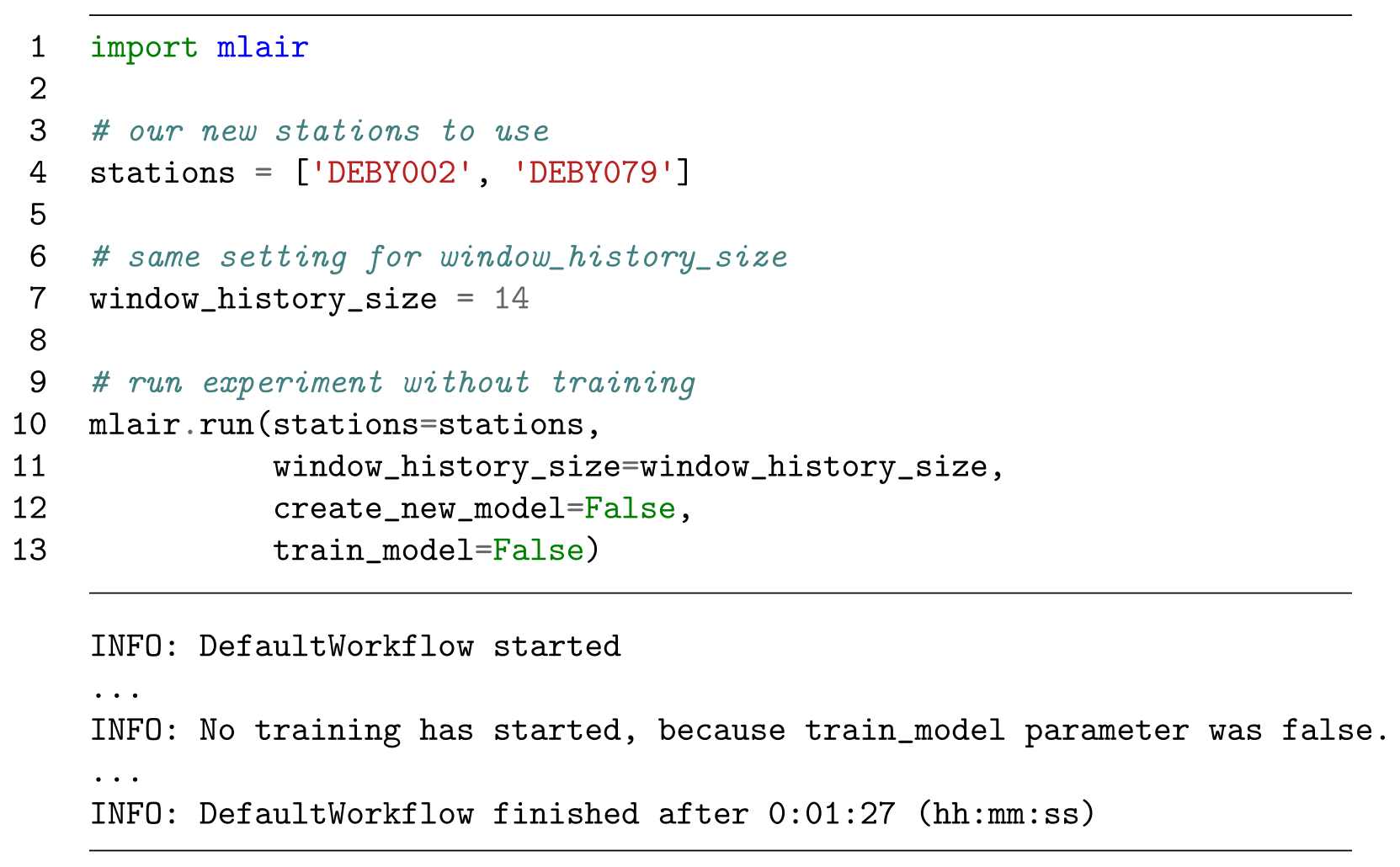
Figure 4Experiment run without training. For this, it is required to have an already trained model in the experiment path.
It is also possible to continue training of an already trained model. If the train_model parameter is set to True, training will be resumed at the last epoch reached previously, if this epoch number is lower than the epochs parameter. Specific uses for this are either an experiment interruption (for example due to wall clock time limit exceedance on batch systems) or the desire to extend the training if the optimal network weights have not been found yet. Further details on training resumption can be found in Sect. 4.9.
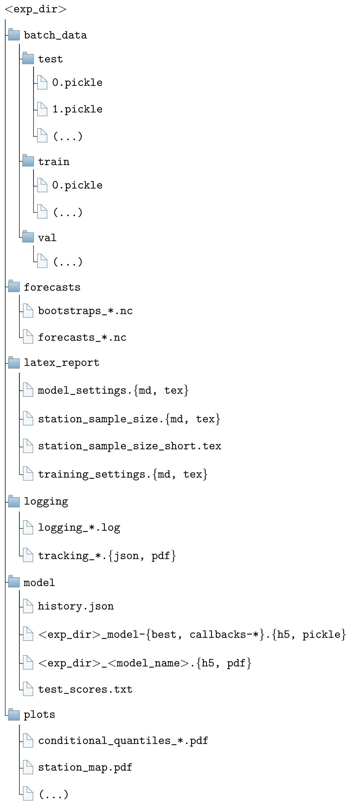
Figure 5Default structure of each MLAir experiment with the subfolders forecasts, latex_report, logging, model, and plots. <exp_dir> is a placeholder for the actual name of the experiment.
3.2 Results of an experiment
All results of an experiment are stored in the directory, which is defined during the experiment setup stage (see Sect. 4.1). The sub-directory structure is created at the beginning of the experiment. There is no automatic deletion of temporary files in case of aborted runs so that the information that is generated up to the program termination can be inspected to find potential errors or to check on a successful initialization of the model, etc. Figure 5 shows the output file structure. The content of each directory is as follows:
-
All samples used for training and validation are stored in the
batch_datafolder. -
forecastscontains the actual predictions of the trained model and the persistence and linear references. All forecasts (model and references) are provided in normalized and original value ranges. Additionally, the optional bootstrap forecasts are stored here (see Sect. 3.3). -
In
latex_report, there are publication-ready tables in Markdown (Gruber, 2004) or LaTeX (LaTeX Project, 2005) format, which give a summary about the stations used, the number of samples, and the hyperparameters and experiment settings. -
The
loggingfolder contains information about the execution of the experiment. In addition to the console output, MLAir also stores messages on the debugging level, which give a better understanding of the internal program sequence. MLAir has a tracking functionality, which can be used to trace which data have been stored and pulled from the central data store. In combination with the corresponding tracking plot that is created at the very end of each experiment automatically, it allows visual tracking of which parameters have an effect on which stage. This functionality is most interesting for developers who make modifications to the source code and want to ensure that their changes do not break the data flow. -
The folder
modelcontains everything that is related to the trained model. Besides the file, which contains the model itself (stored in the binary hierarchical data format HDF5; Koranne, 2011), there is also an overview graphic of the model architecture and all Keras callbacks, for example from the learning rate. If a training is not started from the beginning but is either continued or applied to a pre-trained model, all necessary information like the model or required callbacks must be stored in this subfolder. -
The
plotsdirectory contains all graphics that are created during an experiment. Which graphics are to be created in postprocessing can be determined using theplot_listparameter in the experiment setup. In addition, MLAir automatically generates monitoring plots, for instance of the evolution of the loss during training.
As described in the last bullet point, all plots which are created during an MLAir experiment can be found in the subfolder plots. By default, all available plot types are created. By explicitly naming individual graphics in the plot_list parameter, it is possible to override this behaviour and specify which graphics are created during postprocessing. Additional plots are created to monitor the training behaviour. These graphics are always created when a training session is carried out. Most of the plots which are created in the course of postprocessing are publication-ready graphics with complete legend and resolution of 500 dpi. Custom graphics can be added to MLAir by attaching an additional run module (see Sect. 4.8) which contains the graphic creation methods.
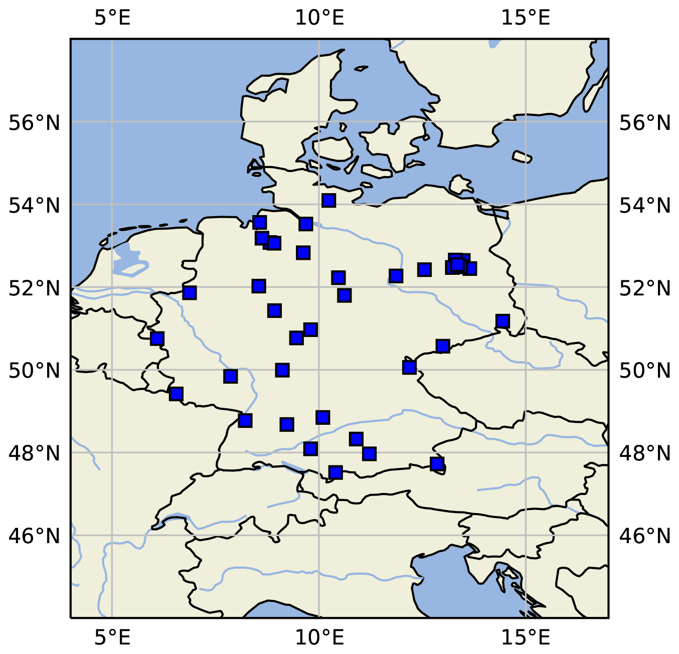
Figure 6Map of central Europe showing the locations of some sample measurement stations as blue squares created by PlotStationMap.
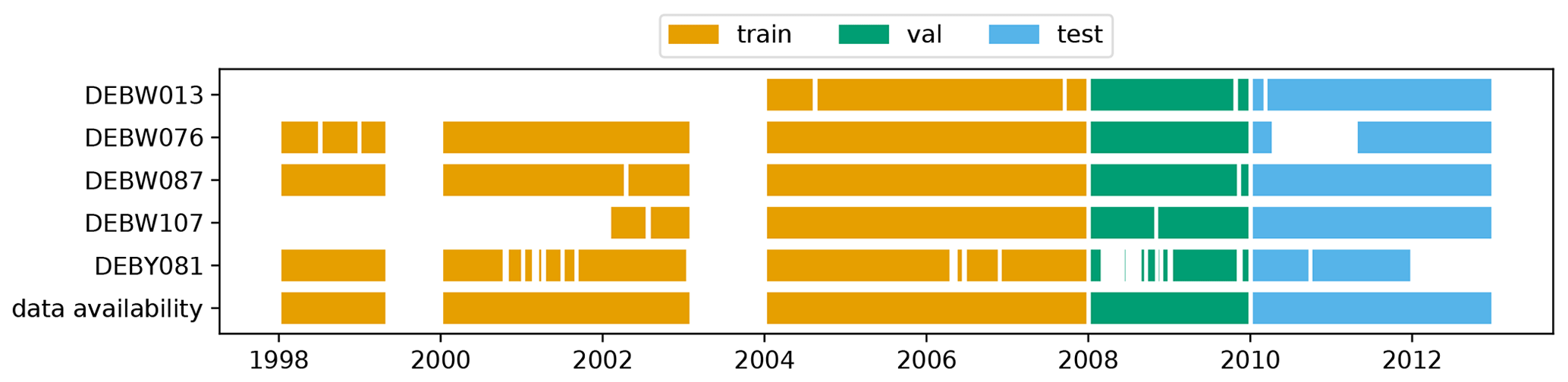
Figure 7PlotAvailability diagram showing the available data for five measurement stations. The different colours denote which period of the time series is used for the training (orange), validation (green), and test (blue) data set. “Data availability” denotes if any of the above-mentioned stations has a data record for a given time.
A general overview of the underlying data can be obtained with the graphics PlotStationMap and PlotAvailability. PlotStationMap (Fig. 6) marks the geographical position of the stations used on a plain map with a land–sea mask, country boundaries, and major water bodies. The data availability chart created by PlotAvailability (Fig. 7) indicates the time periods for which preprocessed data for each measuring station are available. The lowest bar shows whether a station with measurements is available at all for a certain point in time. The three subsets of training, validation, and testing data are highlighted in different colours.
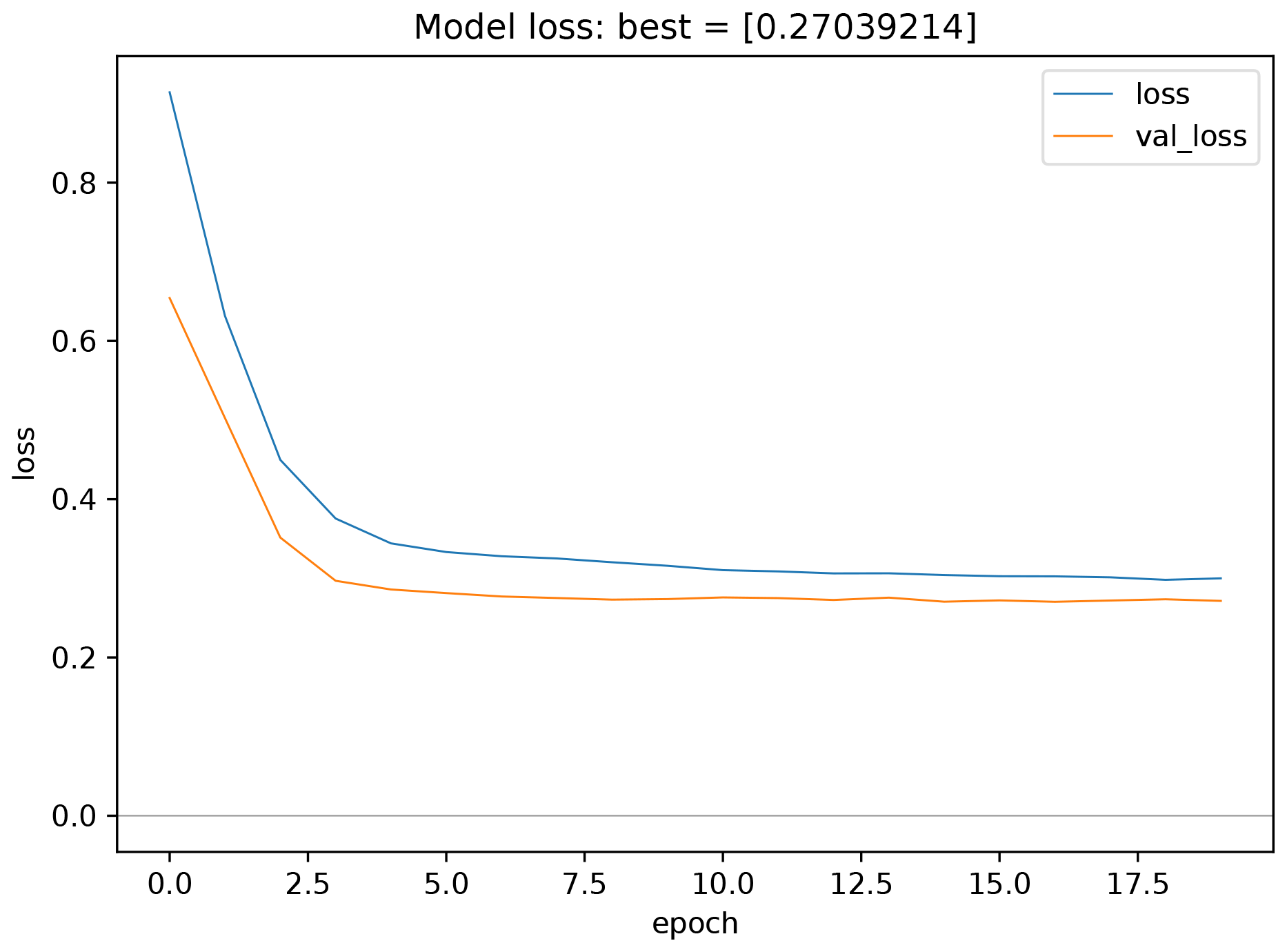
Figure 8Monitoring plots showing the evolution of train and validation loss as a function of the number of epochs. This plot type is kept very simplistic by choice. The underlying data are saved during the experiment so that it would be easy to create a more advanced plot using the same data.
The monitoring graphics show the course of the loss function as well as the error depending on the epoch for the training and validation data (see Fig. 8). In addition, the error of the best model state with respect to the validation data is shown in the plot title. If the learning rate is modified during the course of the experiment, another plot is created to show its development. These monitoring graphics are kept as simple as possible and are meant to provide insight into the training process. The underlying data are always stored in the JavaScript Object Notation format (.json, ISO Central Secretary, 2017) in the subfolder model and can therefore be used for case-specific analyses and plots.

Figure 9Graph of PlotMonthlySummary showing the observations (green) and the predictions for all forecast steps (dark to light blue) separated for each month.
Through the graphs PlotMonthlySummary and PlotTimeSeries it is possible to quickly assess the forecast quality of the ML model. The PlotMonthlySummary (see Fig. 9) summarizes all predictions of the model covering all stations but considering each month separately as a box-and-whisker diagram. With this graph it is possible to get a general overview of the distribution of the predicted values compared to the distribution of the observed values for each month. Besides, the exact course of the time series compared to the observation can be viewed in the PlotTimeSeries (not included as a figure in this article). However, since this plot has to scale according to the length of the time series, it should be noted that this last-mentioned graph is kept very simple and is generally not suitable for publication.
3.3 Statistical analysis of results
A central element of MLAir is the statistical evaluation of the results according to state-of-the-art methods used in meteorology. To obtain specific information on the forecasting model, we treat forecasts and observations as random variables. Therefore, the joint distribution p(m,o) of a model m and an observation o contains information on p(m), p(o) (marginal distribution), and the relations p(o|m) and p(m|o) (conditional distribution) between both of them (Murphy and Winkler, 1987). Following Murphy et al. (1989), marginal distribution is shown as a histogram (light grey), while the conditional distribution is shown as percentiles in different line styles. By using PlotConditionalQuantiles, MLAir automatically creates plots for the entire test period (Fig. 10) that are, as is common in meteorology, separated by seasons.
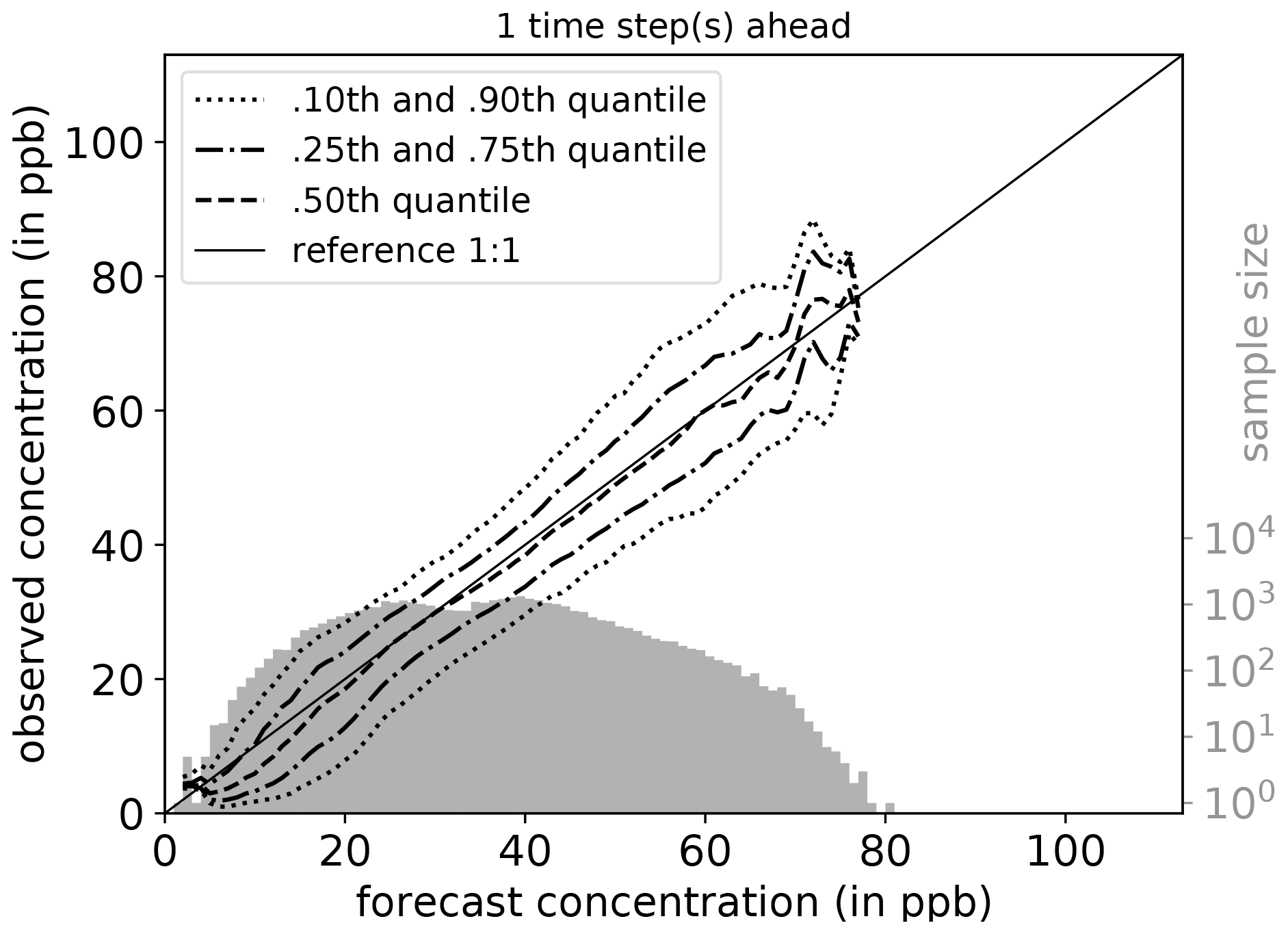
Figure 10Conditional quantiles in terms of calibration-refinement factorization for the first lead time and the full test period. The marginal forecasting distribution is shown as a log histogram in light grey (counting on right axis). The conditional distribution (calibration) is shown as percentiles in different line styles. Calculations are done with a bin size of 1 ppb. Moreover, the percentiles are smoothed by a rolling mean of window size three. This kind of plot was originally proposed by Murphy et al. (1989) and can be created using PlotConditionalQuantiles.
In order to access the genuine added value of a new forecasting model, it is essential to take other existing forecasting models into account instead of reporting only metrics related to the observation. In MLAir we implemented three types of basic reference forecasts: (i) a persistence forecast, (ii) an ordinary multi-linear least square model, and (iii) four climatological forecasts.
The persistence forecast is based on the last observed time step, which is then used as a prediction for all lead times. The ordinary multi-linear least square model serves as a linear competitor and is derived from the same data the model was trained with. For the climatological references, we follow Murphy (1988) who defined single and multiple valued climatological references based on different timescales. We refer the reader to Murphy (1988) for an in-depth discussion of the climatological reference. Note that this kind of persistence and also the climatological forecast might not be applicable for all temporal resolutions and may therefore need adjustment in different experiment settings. We think here, for example, of a clear diurnal pattern in temperature, for which a persistence of successive observations would not provide a good forecast. In this context, a reference forecast based on the observation of the previous day at the same time might be more suitable.
For the comparison, we use a skill score S, which is naturally defined as the performance of a new forecast compared to a competitive reference with respect to a statistical metric (Murphy and Daan, 1985). Applying the mean squared error as the statistical metric, such a skill score S reduces to unity minus the ratio of the error of the forecast to the reference. A positive skill score can be interpreted as the percentage of improvement of the new model forecast in comparison to the reference. On the other hand, a negative skill score denotes that the forecast of interest is less accurate than the referencing forecast. Consequently, a value of zero denotes that both forecasts perform equally (Murphy, 1988).

Figure 11Skill scores of different reference models like persistence (persi) and ordinary multi-linear least square (ols). Skill scores are shown separately for all forecast steps (dark to light blue). This graph is generated by invoking PlotCompetitiveSkillScore.

Figure 12Climatological skill scores (cases I to IV) and related terms of the decomposition as proposed in Murphy (1988) created by PlotClimatologicalSkillScore. Skill scores and terms are shown separately for all forecast steps (dark to light blue). In brief, cases I to IV describe a comparison with climatological reference values evaluated on the test data. Case I is the comparison of the forecast with a single mean value formed on the training and validation data and case II with the (multi-value) monthly mean. The climatological references for cases III and IV are, analogous to cases I and II, the single and the multi-value mean, but on the test data. Cases I to IV are calculated from the terms AI to CIV. For more detailed explanations of the cases, we refer to Murphy (1988).
The PlotCompetitiveSkillScore (Fig. 11) includes the comparison between the trained model, the persistence, and the ordinary multi-linear least squared regression. The climatological skill scores are calculated separately for each forecast step (lead time) and summarized as a box-and-whiskers plot over all stations and forecasts (Fig. 12), and as a simplified version showing the skill score only (not shown) using PlotClimatologicalSkillScore.
In addition to the statistical model evaluation, MLAir also allows the importance of individual input variables to be assessed through bootstrapping of individual input variables. For this, the time series of each individual input variable is resampled n times (with replacement) and then fed to the trained network. By resampling a single input variable, its temporal information is disturbed, but the general frequency distribution is preserved. The latter is important because it ensures that the model is provided only with values from a known range and does not extrapolate out-of-sample. Afterwards, the skill scores of the bootstrapped predictions are calculated using the original forecast as reference. Input variables that show an overly negative skill score during bootstrapping have a stronger influence on the prediction than input variables with a small negative skill score. In case the bootstrapped skill score even reaches the positive value domain, this could be an indication that the examined variable has no influence on the prediction at all. The result of this approach applied to all input variables is presented in PlotBootstrapSkillScore (Fig. 13). A more detailed description of this approach is given in Kleinert et al. (2021).
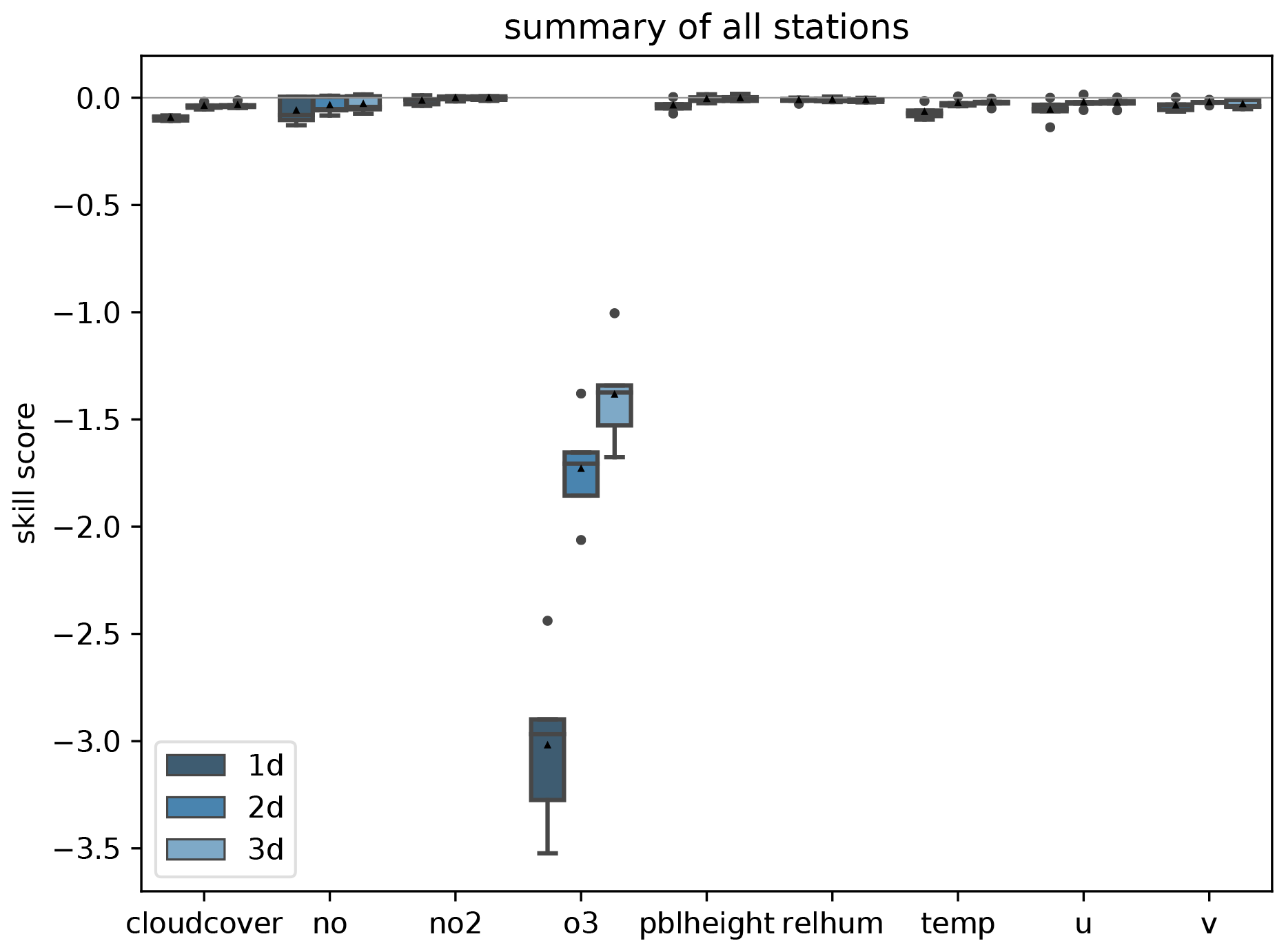
Figure 13Skill score of bootstrapped model input predictions separated for each input variable (x axis) and forecast steps (dark to light blue) with the original (non-bootstrapped) predictions as reference. PlotBootstrapSkillScore is only executed if bootstrap analysis is enabled.
As well as the already described workflow adjustments, MLAir offers a large number of configuration options. Instead of defining parameters at different locations inside the code, all parameters are centrally set in the experiment setup. In this section, we describe all parameters that can be modified and the authors' choices for default settings when using the default workflow of MLAir.
Table 1Summary of all parameters related to the host system that are required, recommended, or optional to adjust for a custom experiment workflow.
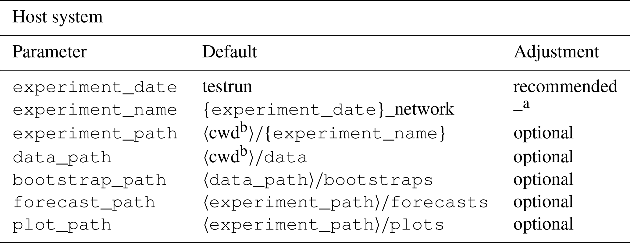
a Only adjustable via the experiment_date parameter.
b Refers to the Linux command to get the path name of the current working directory.
4.1 Host system and processing units
The MLAir workflow can be adjusted to the hosting system. For that, the local paths for experiment and data are adjustable (see Table 1 for all options). Both paths are separated by choice. This has the advantage that the same data can be used multiple times for different experiment setups if stored outside the experiment path. Contrary to the data path placement, all created plots and forecasts are saved in the experiment_path by default, but this can be adjusted through the plot_path and forecast_path parameter.
Concerning the processing units, MLAir supports both central processing units (CPUs) and GPUs. Due to their bandwidth optimization and efficiency on matrix operations, GPUs have become popular for ML applications (see Krizhevsky et al., 2012). Currently, the sample models implemented in MLAir are based on TensorFlow v1.13.1, which has distinct branches: the tensorflow-1.13.1 package for CPU computation and the tensorflow-gpu-1.13.1 package for GPU devices. Depending on the operating system, the user needs to install the appropriate library if using TensorFlow releases 1.15 and older (TensorFlow, 2020). Apart from this installation issue, MLAir is able to detect and handle both TensorFlow versions during run time. An MLAir version to support TensorFlow v2 is planned for the future (see Sect. 5).
4.2 Preprocessing
In the course of preprocessing, the data are prepared to allow immediate use in training and evaluation without further preparation. In addition to the general data acquisition and formatting, which will be discussed in Sect. 4.3 and 4.4, preprocessing also handles the split into training, validation, and test data. All parameters discussed in this section are listed in Table 2.
Table 2Summary of all parameters related to the preprocessing that are required, recommended, or optional to adjust for a custom experiment workflow.
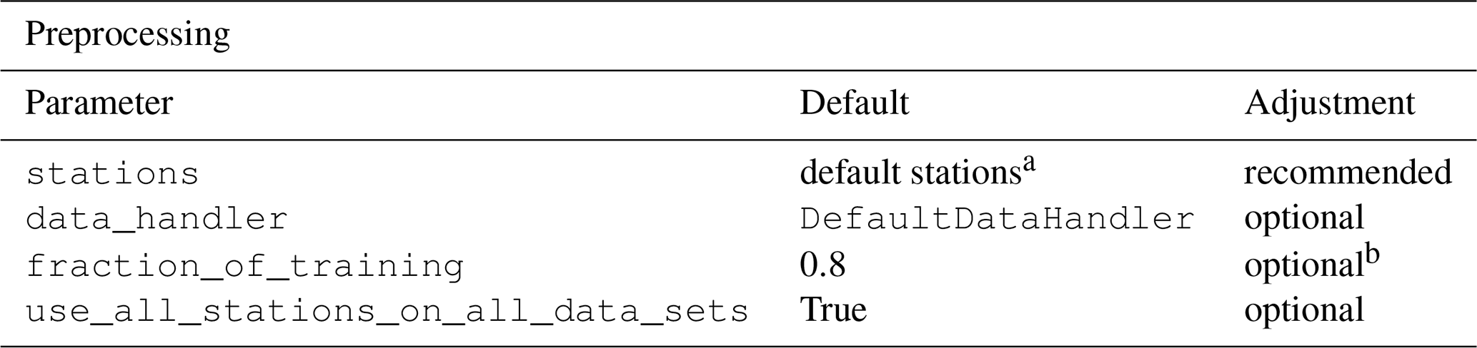
a Default stations: DEBW107, DEBY081, DEBW013, DEBW076, DEBW087.
b Not used in the default setup because use_all_stations_on_all_data_sets is True.
Data are split into subsets along the temporal axis and station between a hold-out data set (called test data) and the data that are used for training (training data) and model tuning (validation data). For each subset, a {train,val,test}_start and {train,val,test}_end date not exceeding the overall time span (see Sect. 4.4) can be set. Additionally, for each subset it is possible to define a minimal number of samples per station {train,val,test}_min_length to remove very short time series that potentially cause misleading results especially in the validation and test phase. A spatial split of the data is achieved by assigning each station to one of the three subsets of data. The parameter fraction_of_training determines the ratio between hold-out data and data for training and validation, where the latter two are always split with a ratio of 80 % to 20 %, which is a typical choice for these subsets.
To achieve absolute statistical data subset independence, data should ideally be split along both temporal and spatial dimensions. Since the spatial dependency of two distinct stations may vary due to weather regimes, season, and time of day (Wilks, 2011), a spatial and temporal division of the data might be useful, as otherwise a trained model can presumably lead to over-confident results. On the other hand, by applying a spatial split in combination with a temporal division, the amount of utilizable data can drop massively. In MLAir, it is therefore up to the user to split data either in the temporal dimension or along both dimensions by using the use_all_stations_on_all_data_sets parameter.
4.3 Custom data handler
The integration of a custom data handler into the MLAir workflow is done by inheritance from the AbstractDataHandler class and implementation of at least the constructor __init__(), and the accessors get_X(), and get_Y(). The custom data handler is added to the MLAir workflow as a parameter without initialization. At runtime, MLAir then queries all the required parameters of this custom data handler from its arguments and keyword arguments, loads them from the data store and finally calls the constructor. If data need to be downloaded or preprocessed, this should be executed inside the constructor. It is sufficient to load the data in the accessor methods if the data can be used without conversion. Note that a data handler is only responsible for preparing data from a single origin, while the iteration and distribution into batches is taken care of while MLAir is running.
The accessor methods for input and target data form a clearly defined interface between MLAir's run modules and the custom data handler. During training the data are needed as a NumPy array; for preprocessing and evaluation the data are partly used as xarray. Therefore the accessor methods have the parameter as_numpy and should be able to return both formats. Furthermore it is possible to use a custom upsampling technique for training. To activate this feature the parameter upsampling can be enabled. If such a technique is not used and therefore not implemented, the parameter has no further effect.
The abstract data handler provides two additional placeholder methods that can support data preparation, training, and validation. Depending on the case, it may be helpful to define these methods within a custom data handler. With the method transformation it is possible to either define or calculate the transformation properties of the data handler before initialization. The returned properties are then applied to all subdata sets, namely training, validation, and testing. Another supporting class method is get_coordinates. This method is currently used only for the map plot for geographical overview (see Sect. 3.2). To feed the overview map, this method must return a dictionary with the geographical coordinates indicated by the keys lat and lon.
Table 3Summary of all parameters related to the default data handler that are required, recommended, or optional to adjust for a custom experiment workflow.
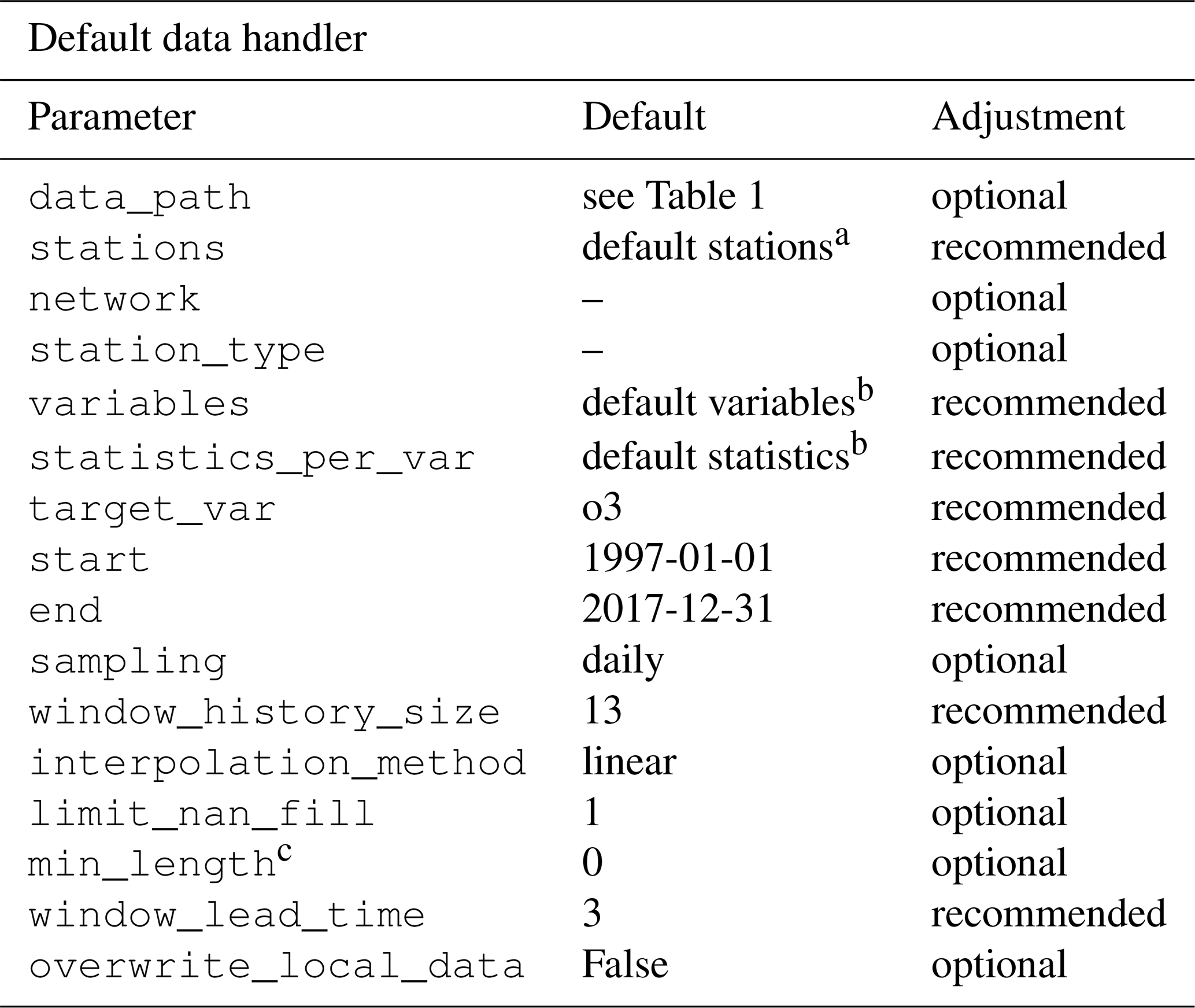
a Default stations: DEBW107, DEBY081, DEBW013, DEBW076, DEBW087.
b Default variables (statistics): o3 (dma8eu), relhum (average_values), temp (maximum), u (average_values), v (average_values), no (dma8eu), no2 (dma8eu), cloudcover (average_values), pblheight (maximum).
c Indicates the required minimum number of samples per station.
4.4 Default data handler
In this section we describe a concrete implementation of a data handler, namely the DefaultDataHandler, using data from the JOIN interface.
Regarding the data handling and preprocessing, several parameters can be set to control the choice of inputs, size of data, etc. in the data handler (see Table 3). First, the underlying raw data must be downloaded from the web. The current version of the DefaultDataHandler is configured for use with the REST API of the JOIN interface (Schultz and Schröder, 2017). Alternatively, data could be already available on the local machine in the directory data_path, e.g. from a previous experiment run. Additionally, a user can force MLAir to load fresh data from the web by enabling the overwrite_local_data parameter. According to the design structure of a data handler, data are handled separately for each observational station indicated by its ID. By default, the DefaultDataHandler uses all German air quality stations provided by the German Environment Agency (Umweltbundesamt, UBA) that are indicated as “background” stations according to the European Environmental Agency (EEA) AirBase classification (European Parliament and Council of the European Union, 2008). Using the stations parameter, a user-defined data collection can be created. To filter the stations, the parameters network and station_type can be used as described in Schultz et al. (2017a) and the documentation of JOIN (Schultz and Schröder, 2017).
For the DefaultDataHandler, it is recommended to specify at least
-
the number of preceding time steps to use for a single input sample (
window_history_size), -
if and which interpolation should be used (
interpolation_method), -
if and how many missing values are allowed to be filled by interpolation (
limit_nan_fill), -
and how many time steps the forecast model should predict (
window_lead_time).
Regarding the data content itself, each requested variable must be added to the variables list and be part of the statistics_per_var dictionary together with a proper statistic abbreviation (see documentation of Schultz and Schröder, 2017). If not provided, both parameters are chosen from a standard set of variables and statistics. Similar actions are required for the target variable. Firstly, target variables are defined in target_var, and secondly, the target variable must also be part of the statistics_per_var parameter. Note that the JOIN REST API calculates these statistics online from hourly values, thereby taking into account a minimum data coverage criterion. Finally, the overall time span the data shall cover can be defined via start and end, and the temporal resolution of the data is set by a string like "daily" passed to the sampling parameter. At this point, we want to refer to Sect. 5, where we discuss the temporal resolution currently available.
4.5 Defining a model class
The motivation behind using model classes was already explained in Sect. 2.4. Here, we show more details on the implementation and customization.
To achieve the goal of an easy plug-and-play behaviour, each ML model implemented in MLAir must inherit from the AbstractModelClass, and the methods set_model and set_compile_options are required to be overwritten for the custom model. Inside set_model, the entire model from inputs to outputs is created. Thereby it has to be ensured that the model is compatible with Keras to be compiled. MLAir supports both the functional and sequential Keras application programming interfaces. For details on how to create a model with Keras, we refer to the official Keras documentation (Chollet et al., 2015). All options for the model compilation should be set in the set_compile_options method. This method should at least include information on the training algorithm (optimizer), and the loss to measure performance during training and optimize the model for (loss). Users can add other compile options like the learning rate (learning_rate), metrics to report additional informative performance metrics, or options regarding the weighting as loss_weights, sample_weight_mode, or weighted_metrics. Finally, methods that are not part of Keras or TensorFlow like customized loss functions or self-made model extensions are required to be added as so-called custom_objects to the model so that Keras can properly use these custom objects. For that, it is necessary to call the set_custom_objects method with all custom objects as key value pairs. See also the official Keras documentation for further information on custom objects.

Figure 14Example how to create a custom ML model implemented as a model class. MyCustomisedModel has a single 1×1 convolution layer followed by two fully connected layers with a neuron size of 16, and the number of forecast steps. The model itself is defined in the set_model method, whereas compile options such as the optimizer, loss, and error metrics are defined in set_compile_options. Additionally, for demonstration, the loss is added as custom object which is not required because a Keras built-in function is used as loss.
An example implementation of a small model using a single convolution and three fully connected layers is shown in Fig. 14. By inheriting from the AbstractModelClass (l. 9), invoking its constructor (l. 15), defining the methods set_model (l. 25–35) and set_compile_options (l. 37–41), and calling these two methods (l. 21–22), the custom model is immediately usable for MLAir. Additionally, the loss is added to the custom objects (l. 23). This last step would not be necessary in this case, because an error function incorporated in Keras is used (l. 2/40). For the purpose of demonstrating how to use a customized loss, it is added nevertheless.
A more elaborate example is described in Kleinert et al. (2021), who used extensions to the standard Keras library in their workflow. So-called inception blocks (Szegedy et al., 2015) and a modification of the two-dimensional padding layers were implemented as Keras layers and could be used in the model afterwards.
Table 4Summary of all parameters related to the training that are required, recommended, or optional to adjust for a custom experiment workflow.
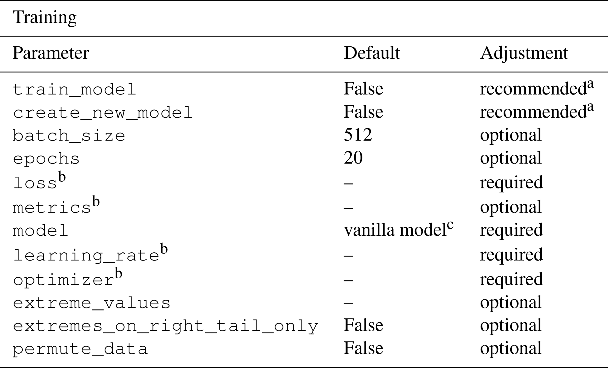
a Note: both parameters are disabled per default to prevent unintended overwriting of a model. If, upon reversion, these parameters are not enabled on the first execution of a new experiment without providing a suitable and trained ML model, the MLAir workflow is going to fail.
b These parameters are set in the model class.
c As default, a vanilla feed-forward neural network architecture will be loaded for workflow testing. The usage of such a simple network for a real application is at least questionable.
4.6 Training
The parameter create_new_model instructs MLAir to create a new model and use it in the training. This is necessary, for example, for the very first training run in a new experiment. However, it must be noted that already existing training progress within the experiment will be overwritten by activating create_new_model. Independent of using a new or already existing model, train_model can be used to set whether the model is to be trained or not. Further notes on the continuation of an already started training or the use of a pre-trained model can be found in Sect. 4.9.
Most parameters to set for the training stage are related to hyperparameter tuning (see Table 4). Firstly, the batch_size can be set. Furthermore, the number of epochs to train needs to be adjusted. Last but not least, the model used itself must be provided to MLAir including additional hyperparameters like the learning_rate, the algorithm to train the model (optimizer), and the loss function to measure model performance. For more details on how to implement an ML model properly we refer to Sect. 4.5.
Due to its application focus on meteorological time series and therefore on solving a regression problem, MLAir offers a particular handling of training data. A popular technique in ML, especially in the image recognition field, is to augment and randomly shuffle data to produce a larger number of input samples with a broader variety. This method requires independent and identically distributed data. For meteorological applications, these techniques cannot be applied out of the box, because of the lack of statistical independence of most data and autocorrelation (see also Schultz et al., 2021). To avoid generating over-confident forecasts, training and test data are split into blocks so that little or no overlap remains between the data sets. Another common problem in ML, not only in the meteorological context, is the natural under-representation of extreme values, i.e. an imbalance problem. To address this issue, MLAir allows more emphasis to be placed on such data points. The weighting of data samples is conducted by an over-representation of values that can be considered as extreme regarding the deviation from a mean state in the output space. This can be applied during training by using the extreme_values parameter, which defines a threshold value at which a value is considered extreme. Training samples with target values that exceed this limit are then used a second time in each epoch. It is also possible to enter more than one value for the parameter. In this case, samples with values that exceed several limits are duplicated according to the number of limits exceeded. For positively skewed distributions, it could be helpful to apply this over-representation only on the right tail of the distribution (extremes_on_right_tail_only). Furthermore, it is possible to shuffle data within, and only within, the training subset randomly by enabling permute_data.
4.7 Validation
The configuration of the ML model validation is related to the postprocessing stage. As mentioned in Sect. 2.3, in the default configuration there are three major validation steps undertaken after each run besides the creation of graphics: first, the trained model is opposed to the two reference models, a simple linear regression and a persistence prediction. Second, these models are compared with climatological statistics. Lastly, the influence of each input variable is estimated by a bootstrap procedure.
Table 5Summary of all parameters related to the evaluation that are required, recommended, or optional to adjust for a custom experiment workflow.
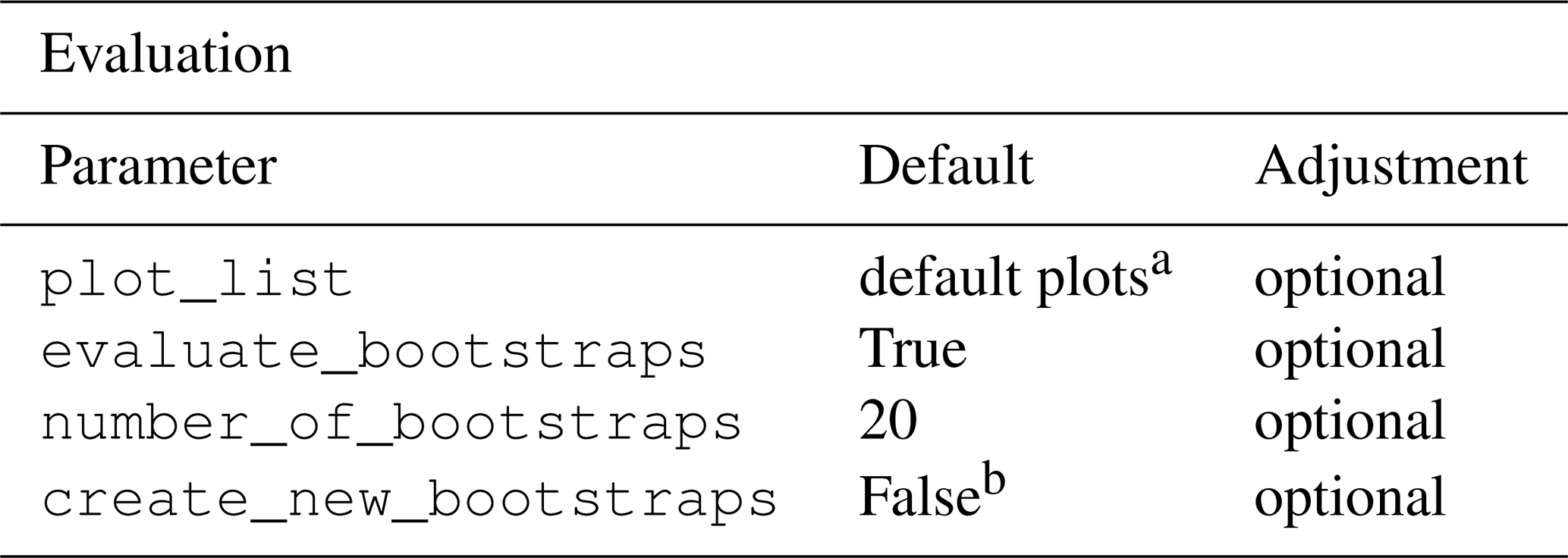
a Default plots are PlotMonthlySummary, PlotStationMap, PlotClimatologicalSkillScore, PlotTimeSeries, PlotCompetitiveSkillScore, PlotBootstrapSkillScore, PlotConditionalQuantiles, and PlotAvailability.
b Is automatically enabled if parameter train_model (see Table 4) is enabled.
Due to the computational burden the calculation of the input variable sensitivity can be skipped and the graphics creation part can be shortened. To perform the sensitivity study, the parameter evaluate_bootstraps must be enabled and the number_of_bootstraps defines how many samples shall be drawn for the evaluation (see Table 5). If such a sensitivity study was already performed and the training stage was skipped, the create_new_bootstraps parameter should be set to False to reuse already preprocessed samples if possible. To control the creation of graphics, the parameter plot_list can be adjusted. If not specified, a default selection of graphics is generated. When using plot_list, each graphic to be drawn must be specified individually. More details about all possible graphics have already been provided in Sect. 3.2 and 3.3. In the current version, extending the validation as part of MLAir's default postprocessing stage is somewhat complicated, but it is possible to append another run module to the workflow to perform additional validations.
4.8 Custom run modules and workflow adaptions
MLAir offers the possibility to define and execute a custom workflow for situations in which special calculations or data evaluation procedures not available in the standard version are needed. For this purpose it is not necessary to modify the program code of MLAir, but instead user-defined run modules can be included in a new workflow. This is done in analogy to the procedure of defining new model classes by inheritance from the base class RunEnvironment. Compared to the very simple examples from Sect. 3, such a use of MLAir requires a slightly increased effort. The implementation of the run module is done straightforwardly by a constructor method, which initializes the module and executes all desired calculation steps when called. To execute the custom workflow, the MLAir Workflow class must be loaded and then each run module must be registered. The order in which the individual stages are added determines the execution sequence.
As custom workflows will generally be necessary if a custom run module is to be defined, we briefly describe how the central data store mentioned in Sect. 2.3 interacts with the workflow module. With the data store it is possible to share any kind of information from previous or subsequent stages. By invoking the constructor of the super class during the initialization of a custom run module, the data store is automatically connected with this module. Information can then be set or queried using the accessor methods get and set. For each saved information object a separate namespace called scope can be assigned. If not specified, the object is always stored in the general scope. If the scope is specified, a separate sub-scope is created. Information stored in this scope memory cannot be accessed from the general scope memory, but conversely all sub-scopes have access to the general scope. For example, more general objects can be set in the general scope and objects specific to a sub-data set, such as test data, can be stored under the scope test. If some objects for the keyword test are retrieved from the data store, then for non-existent objects in the test namespace attributes from the general scope are used if available.
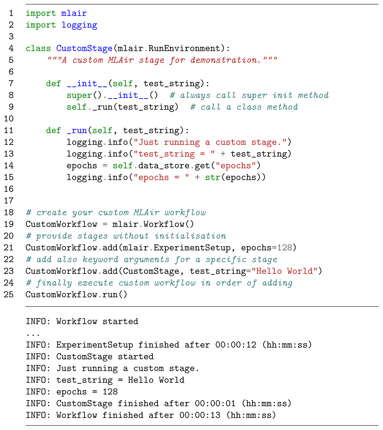
Figure 15Embedding of a custom run module in a modified MLAir workflow. In comparison to Figs. 2, 3, and 4, this code example works on a single step deeper regarding the level of abstraction. Instead of calling the run method of MLAir, the user needs to add all stages individually and is responsible for all dependencies between the stages. By using the Workflow class as context manager, all stages are automatically connected with the result that all stages can easily be plugged in.
An example for the implementation of a custom run module embedded in a custom workflow can be found in Fig. 15. The custom run module named CustomStage inherits from the base class RunEnvironment (l. 4) and calls its constructor (l. 8) on initialization. The CustomStage expects a single parameter (test_string, l. 7), which is used during the run method (l. 11–15). The run method first logs two information messages by using the test_string parameter (l. 12–13). Then it extracts the value of the parameter epochs (l. 14) that has been set in the ExperimentSetup (l. 21) from the data store and logs the value of this parameter too. To run this custom run module is has to be included in a workflow. First an empty workflow is created (l. 19) and then individual run modules are attached (l. 21–23). As last step, this new defined workflow is executed by calling the run method (l. 25).
4.9 How to continue an experiment?
There can be different reasons for the continuation of an experiment. First of all, by looking at the monitoring graphs, it could be discovered that training has not yet converged and the number of epochs should be increased. Instead of training a new network from scratch, the training can be resumed from the latest epoch to save time. To do so, the parameter epochs must be increased accordingly and create_new_model must be set to False. If the model output folder has not been touched, the intermediate results and the history of the previous training are usually available in full, so that MLAir can continue the training as if it had never been interrupted. Another reason for a continuation would be the interruption of the training for unexpected reasons such as runtime exceedance on batch systems. By keeping the same number of epochs and switching off the creation of a new model, the training continues at the last checkpoint (see model setup in Sect. 2.3). Finally, MLAir can also be used in the context of transfer learning. By providing a pre-trained model and having train_model enabled and create_new_model disabled, a transfer learning task can be performed.
Even though MLAir addresses a wide range of ML-related problems and allows many different ML architectures and customized workflows to be embedded, it is still no universal Swiss Army knife but rather focuses on the application of neural networks for the task of station time series forecasting. In this section we will explain the limitations of MLAir and why MLAir ends at these points.
Due to the scientifically oriented development of MLAir starting from a specific research question (Kleinert et al., 2021), MLAir could initially only use data from the REST API of JOIN. This binding has already been revoked in the current version, however, the DefaultDataHandler still uses this data source. Furthermore, MLAir always expects a particular structure in the data and especially considers the data as a collection of time series data from various stations. We are currently investigating the possibility of integrating grid data, which could be taken from a weather model, and time-constant data such as topography into the MLAir workflow, but we cannot yet present any results on how easy such an integration would be.
While MLAir can technically handle data in different time resolutions, it has been tested primarily on daily aggregated data due to the specific science case which served as the seed for its development. The use of different temporal resolutions was spot-checked and could be successfully confirmed without obvious errors, but we cannot guarantee that the results will be meaningful if data in other temporal resolutions are used as inputs. In particular, most of the evaluation routines may not make sense for data in less than hourly or greater than daily resolution. Note also that MLAir does not perform explicit error checking or missing value handling. Such functionality must be implemented within the data handler. MLAir expects a ready-to-use data set without missing values provided by the data handler during training.
Another limitation is the choice of the underlying libraries and their versions. Due to the selection of TensorFlow as back-end, it is not possible to use PyTorch or other frameworks in combination with MLAir. Specifically, MLAir was developed and tested with TensorFlow version 1.13.1, as the HPC systems on which our experiments are performed supported this version at the time of writing. We have already tested MLAir occasionally with the TensorFlow version 1.15 and could not find any errors. Please check the code repository for updates concerning the support of newer TensorFlow versions, which we hope to make available in the coming months.
MLAir is an innovative software package intended to facilitate high-quality meteorological studies using ML. By providing an end-to-end solution based on a specific scientific workflow of time series prediction, MLAir enables a transparent and reproducible conduction of ML experiments in this domain. Due to the plug-and-play behaviour it is straightforward to explore different model architectures and change various aspects of the workflow or model evaluation. Although MLAir is focusing on neural networks, it should be possible to include other ML techniques. Since MLAir is based on a pure Python environment, and it is highly portable. It has been tested on various computing systems from desktop workstations to high-end supercomputers.
MLAir is under continuous development. Further enhancements of the program are already planned and can be found in the issue tracker (see Code availability). Ongoing developments concern the extension of the statistical evaluation methods, the graphical presentation of the results, and the flawless support of temporal resolutions other than daily aggregated data. Through further code refactoring, MLAir will become even more versatile as the decoupling of individual components is being pushed forward. In particular, it is planned to structure the data handling in a more modular way so that varying structured data sources can be connected and used without much effort. We invite the community of meteorological ML scientists to participate in the further development of MLAir through comments and contributions to code and documentation. A good starting point for contributions is the issue tracker of MLAir.
We hope that MLAir can serve as a blueprint for the development of reusable ML applications in the fields of meteorology and air quality, as it seeks to combine the best practices from ML with the best practices of meteorological model evaluation and data preprocessing. MLAir is thus a contribution to strengthen cooperation between the communities of ML and meteorology or air quality researchers.
The current version of MLAir is available from the project website https://gitlab.version.fz-juelich.de/toar/mlair (last access: 10 March 2021) under the MIT licence. The exact version v1.0.0 of MLAir described in this paper and used to produce the code examples shown is archived on B2SHARE (Leufen et al., 2020, https://doi.org/10.34730/5a6c3533512541a79c5c41061743f5e3). Detailed installation instructions are provided in the project page readme file. There is also a Jupyter notebook with all code snippets to reproduce the examples highlighted in this paper.
MLAir is not directly linked to any specific data. Data used in the examples are extracted from the corresponding databases at runtime, as described and cited in the text.
The concept of MLAir was developed by LHL. Detailed investigations on methodological approaches were carried out by LHL and FK. FK contributed the first use case. The actual implementation of the software and its validation and visualization were done by LHL and FK. LHL was responsible for the code structure and test developments. MGS contributed to the concept discussions and provided supervision and funding. LHL wrote the original draft, all authors reviewed the manuscript and helped in the preparation of the final paper as well as drafting the responses to the reviewers' comments.
The authors declare that they have no conflict of interest.
The authors gratefully acknowledge the Jülich Supercomputing Centre for providing the infrastructure and resources to develop this software.
This research has been supported by the European Research Council, H2020 Research Infrastructures (IntelliAQ (grant no. 787576).
The article processing charges for this open-access
publication were covered by a Research
Centre of the Helmholtz Association.
This paper was edited by Christoph Knote and reviewed by two anonymous referees.
Abadi, M., Agarwal, A., Barham, P., Brevdo, E., Chen, Z., Citro, C., Corrado, G. S., Davis, A., Dean, J., Devin, M., Ghemawat, S., Goodfellow, I., Harp, A., Irving, G., Isard, M., Jia, Y., Jozefowicz, R., Kaiser, L., Kudlur, M., Levenberg, J., Mané, D., Monga, R., Moore, S., Murray, D., Olah, C., Schuster, M., Shlens, J., Steiner, B., Sutskever, I., Talwar, K., Tucker, P., Vanhoucke, V., Vasudevan, V., Viégas, F., Vinyals, O., Warden, P., Wattenberg, M., Wicke, M., Yu, Y., and Zheng, X.: TensorFlow: Large-Scale Machine Learning on Heterogeneous Systems, available at: https://www.tensorflow.org/ (last access: 10 March 2021), 2015. a
Bentayeb, M., Wagner, V., Stempfelet, M., Zins, M., Goldberg, M., Pascal, M., Larrieu, S., Beaudeau, P., Cassadou, S., Eilstein, D., Filleul, L., Le Tertre, A., Medina, S., Pascal, L., Prouvost, H., Quénel, P., Zeghnoun, A., and Lefranc, A.: Association between long-term exposure to air pollution and mortality in France: a 25-year follow-up study, Environ. Int., 85, 5–14, https://doi.org/10.1016/j.envint.2015.08.006, 2015. a
Bishop, C. M.: Pattern recognition and machine learning, Springer, New York, 2006. a
Brunner, D., Savage, N., Jorba, O., Eder, B., Giordano, L., Badia, A., Balzarini, A., Baró, R., Bianconi, R., Chemel, C., Curci, G., Forkel, R., Jiménez-Guerrero, P., Hirtl, M., Hodzic, A., Honzak, L., Im, U., Knote, C., Makar, P., Manders-Groot, A., van Meijgaard, E., Neal, L., Pérez, J. L., Pirovano, G., San Jose, R., Schröder, W., Sokhi, R. S., Syrakov, D., Torian, A., Tuccella, P., Werhahn, J., Wolke, R., Yahya, K., Zabkar, R., Zhang, Y., Hogrefe, C., and Galmarini, S.: Comparative analysis of meteorological performance of coupled chemistry-meteorology models in the context of AQMEII phase 2, Atmos. Environ., 115, 470–498, https://doi.org/10.1016/j.atmosenv.2014.12.032, 2015. a
Cho, K., van Merrienboer, B., Gulcehre, C., Bahdanau, D., Bougares, F., Schwenk, H., and Bengio, Y.: Learning Phrase Representations using RNN Encoder-Decoder for Statistical Machine Translation, arXiv: 1406.1078, available at: http://arxiv.org/abs/1406.1078 (last access: 10 March 2021), 2014. a
Chollet, F., et al.: Keras, available at: https://keras.io (last access: 10 March 2021), 2015. a, b
Cohen, A. J., Anderson, H. R., Ostro, B., Pandey, K. D., Krzyzanowski, M., Künzli, N., Gutschmidt, K., Pope, A., Romieu, I., Samet, J. M., and Smith, K.: The Global Burden of Disease Due to Outdoor Air Pollution, J. Toxicol. Env. Hea. A, 68, 1301–1307, https://doi.org/10.1080/15287390590936166, 2005. a
Elliott, T.: The State of the Octoverse: machine learning, The GitHub Blog, available at: https://github.blog/2019-01-24-the-state-of-the-octoverse-machine-learning/, (last access: 23 June 2020), 2019. a
European Parliament and Council of the European Union: Directive 2008/50/EC of the European Parliament and of the Council of 21 May 2008 on ambient air quality and cleaner air for Europe, Official Journal of the European Union, available at: http://data.europa.eu/eli/dir/2008/50/oj (last access: 10 March 2021), 2008. a
Goodfellow, I., Pouget-Abadie, J., Mirza, M., Xu, B., Warde-Farley, D., Ozair, S., Courville, A., and Bengio, Y.: Generative Adversarial Nets, in: Advances in Neural Information Processing Systems 27, edited by: Ghahramani, Z., Welling, M., Cortes, C., Lawrence, N. D., and Weinberger, K. Q., pp. 2672–2680, Curran Associates, Inc., available at: http://papers.nips.cc/paper/5423-generative-adversarial-nets.pdf (last access: 10 March 2021), 2014. a
Goodfellow, I., Bengio, Y., and Courville, A.: Deep Learning, MIT Press, http://www.deeplearningbook.org (last access: 10 March 2021), 2016. a
Gruber, J.: Markdown, available at: https://daringfireball.net/projects/markdown/license, (last access: 7 January 2021), 2004. a
Hochreiter, S. and Schmidhuber, J.: Long Short-Term Memory, Neural Computation, 9, 1735–1780, https://doi.org/10.1162/neco.1997.9.8.1735, 1997. a
Hoyer, S. and Hamman, J.: xarray: N-D labeled arrays and datasets in Python, J. Open Res. Softw., 5, 10, https://doi.org/10.5334/jors.148, 2017. a
Hoyer, S., Hamman, J., Roos, M., Fitzgerald, C., Cherian, D., Fujii, K., Maussion, F., crusaderky, Kleeman, A., Kluyver, T., Clark, S., Munroe, J., keewis, Hatfield-Dodds, Z., Nicholas, T., Abernathey, R., Wolfram, P. J., MaximilianR, Hauser, M., Markel, Gundersen, G., Signell, J., Helmus, J. J., Sinai, Y. B., Cable, P., Amici, A., lumbric, Rocklin, M., Rivera, G., and Barna, A.: pydata/xarray v0.15.0, Zenodo, https://doi.org/10.5281/zenodo.3631851, 2020. a
ISO Central Secretary: Information technology – The JSON data interchange syntax, Standard ISO/IEC 21778:2017, International Organization for Standardization, Geneva, Switzerland, available at: https://www.iso.org/standard/71616.html (last access: 10 March 2021), 2017. a
Kingma, D. P. and Welling, M.: Auto-Encoding Variational Bayes, arXiv: 1312.6114, available at: https://arxiv.org/abs/1312.6114 (last access: 10 March 2021), 2014. a
Kleinert, F., Leufen, L. H., and Schultz, M. G.: IntelliO3-ts v1.0: a neural network approach to predict near-surface ozone concentrations in Germany, Geosci. Model Dev., 14, 1–25, https://doi.org/10.5194/gmd-14-1-2021, 2021. a, b, c
Kluyver, T., Ragan-Kelley, B., Pérez, F., Granger, B., Bussonnier, M., Frederic, J., Kelley, K., Hamrick, J., Grout, J., Corlay, S., Ivanov, P., Avila, D., Abdalla, S., Willing, C., and development team, J.: Jupyter Notebooks – a publishing format for reproducible computational workflows, in: Positioning and Power in Academic Publishing: Players, Agents and Agendas, edited by: Loizides, F. and Scmidt, B., IOS Press, the Netherlands, 87–90, available at: https://eprints.soton.ac.uk/403913/ (last access: 10 March 2021), 2016. a
Koranne, S.: Hierarchical data format 5: HDF5, in: Handbook of Open Source Tools, 191–200, Springer, Boston, MA, HDF5 is maintained by The HDF Group, http://www.hdfgroup.org/HDF5 (last access: 10 March 2021), 2011. a
Krizhevsky, A., Sutskever, I., and Hinton, G. E.: ImageNet Classification with Deep Convolutional Neural Networks, in: Advances in Neural Information Processing Systems 25, edited by: Bartlett, P. L., Pereira, F. C. N., Burges, C. J. C., Bottou, L., and Weinberger, K. Q., Curran Associates, Inc., 1106–1114, available at: http://papers.nips.cc/paper/4824-imagenet-classification-with-deep-convolutional-neural-networks (last access: 10 March 2021), 2012. a
LaTeX Project: LaTeX, available at: https://www.latex-project.org/, (last access: 7 January 2021), 2005. a
Lecun, Y., Bottou, L., Bengio, Y., and Haffner, P.: Gradient-based learning applied to document recognition, Proceedings of the IEEE, 86, 2278–2324, https://doi.org/10.1109/5.726791, 1998. a
Lefohn, A. S., Malley, C. S., Smith, L., Wells, B., Hazucha, M., Simon, H., Naik, V., Mills, G., Schultz, M. G., Paoletti, E., De Marco, A., Xu, X., Zhang, L., Wang, T., Neufeld, H. S., Musselman, R. C., Tarasick, D., Brauer, M., Feng, Z., Tang, H., Kobayashi, K., Sicard, P., Solberg, S., and Gerosa, G.: Tropospheric ozone assessment report: Global ozone metrics for climate change, human health, and crop/ecosystem research, Elementa: Science of the Anthropocene, 1, 1, https://doi.org/10.1525/elementa.279, 2018. a
Leufen, L. H., Kleinert, F., and Schultz, M. G.: MLAir (v1.0.0) – a tool to enable fast and flexible machine learning on air data time series – Source Code, EUDAT Collaborative Data Infrastructure, https://doi.org/10.34730/fcc6b509d5394dad8cfdfc6e9fff2bec, 2020. a
Mills, G., Pleijel, H., Malley, C., Sinha, B., Cooper, O., Schultz, M., Neufeld, H., Simpson, D., Sharps, K., Feng, Z., Gerosa, G., Harmens, H., Kobayashi, K., Saxena, P., Paoletti, E., Sinha, V., and Xu, X.: Tropospheric Ozone Assessment Report: Present-day tropospheric ozone distribution and trends relevant to vegetation, Elementa: Science of the Anthropocene, 6, 47, https://doi.org/10.1525/elementa.302, 2018. a
Murphy, A. H.: Skill Scores Based on the Mean Square Error and Their Relationships to the Correlation Coefficient, Mon. Weather Rev., 116, 2417–2424, https://doi.org/10.1175/1520-0493(1988)116<2417:SSBOTM>2.0.CO;2, 1988. a, b, c, d, e
Murphy, A. H. and Daan, H.: Forecast evaluation, in: Probability, statistics, and decision making in the atmospheric sciences, edited by: Murphy, A. H. and Katz, R. W., Westview Press, Boulder, USA, 379–437, 1985. a
Murphy, A. H. and Winkler, R. L.: A General Framework for Forecast Verification, Mon. Weather Rev., 115, 1330–1338, https://doi.org/10.1175/1520-0493(1987)115<1330:AGFFFV>2.0.CO;2, 1987. a
Murphy, A. H., Brown, B. G., and Chen, Y.-S.: Diagnostic Verification of Temperature Forecasts, Weather Forecast., 4, 485–501, https://doi.org/10.1175/1520-0434(1989)004<0485:DVOTF>2.0.CO;2, 1989. a, b
Musgrave, K., Belongie, S., and Lim, S.-N.: A Metric Learning Reality Check, arXiv: 2003.08505, available at: https://arxiv.org/abs/2003.08505 (last access: 10 March 2021), 2020. a
Paszke, A., Gross, S., Massa, F., Lerer, A., Bradbury, J., Chanan, G., Killeen, T., Lin, Z., Gimelshein, N., Antiga, L., Desmaison, A., Kopf, A., Yang, E., DeVito, Z., Raison, M., Tejani, A., Chilamkurthy, S., Steiner, B., Fang, L., Bai, J., and Chintala, S.: PyTorch: An Imperative Style, High-Performance Deep Learning Library, in: Advances in Neural Information Processing Systems 32, edited by: Wallach, H., Larochelle, H., Beygelzimer, A., d'Alché-Buc, F., Fox, E., and Garnett, R., Curran Associates, Inc., Vancouver, Canada, 8024–8035, available at: http://papers.neurips.cc/paper/9015-pytorch-an-imperative-style-high-performance-deep-learning-library.pdf (last access: 10 March 2021), 2019. a
Python Software Foundation: Python Language Reference, release 3.6.8, PEP 494, available at: https://www.python.org/dev/peps/pep-0494/ (last access: 10 March 2021), 2018. a
Reback, J., McKinney, W., jbrockmendel, Van den Bossche, J., Augspurger, T., Cloud, P., gfyoung, Sinhrks, Klein, A., Roeschke, M., Tratner, J., She, C., Hawkins, S., Ayd, W., Petersen, T., Schendel, J., Hayden, A., Garcia, M., MomIsBestFriend, Jancauskas, V., Battiston, P., Seabold, S., chris-b1, h-vetinari, Hoyer, S., Overmeire, W., alimcmaster1, Mehyar, M., Dong, K., and Whelan, C.: pandas-dev/pandas: Pandas v1.0.1, Zenodo, https://doi.org/10.5281/zenodo.3644238, 2020. a
Rezende, D. J., Mohamed, S., and Wierstra, D.: Stochastic Backpropagation and Approximate Inference in Deep Generative Models, arXiv: 1401.4082, available at: https://arxiv.org/abs/1401.4082 (last access: 10 March 2021), 2014. a
Schultz, M. G. and Schröder, S.: Documentation of the JOIN REST interface, Juelich, Germany, available at: https://join.fz-juelich.de/services/rest/surfacedata/, (last access: 18 September 2020), 2017. a, b, c
Schultz, M. G., Schröder, S., Lyapina, O., Cooper, O. R., Galbally, I., Petropavlovskikh, I., von Schneidemesser, E., Tanimoto, H., Elshorbany, Y., Naja, M., Seguel, R. J., Dauert, U., Eckhardt, P., Feigenspan, S., Fiebig, M., Hjellbrekke, A.-G., Hong, Y.-D., Kjeld, P. C., Koide, H., Lear, G., Tarasick, D., Ueno, M., Wallasch, M., Baumgardner, D., Chuang, M.-T., Gillett, R., Lee, M., Molloy, S., Moolla, R., Wang, T., Sharps, K., Adame, J. A., Ancellet, G., Apadula, F., Artaxo, P., Barlasina, M. E., Bogucka, M., Bonasoni, P., Chang, L., Colomb, A., Cuevas-Agulló, E., Cupeiro, M., Degorska, A., Ding, A., Fröhlich, M., Frolova, M., Gadhavi, H., Gheusi, F., Gilge, S., Gonzalez, M. Y., Gros, V., Hamad, S. H., Helmig, D., Henriques, D., Hermansen, O., Holla, R., Hueber, J., Im, U., Jaffe, D. A., Komala, N., Kubistin, D., Lam, K.-S., Laurila, T., Lee, H., Levy, I., Mazzoleni, C., Mazzoleni, L. R., McClure-Begley, A., Mohamad, M., Murovec, M., Navarro-Comas, M., Nicodim, F., Parrish, D., Read, K. A., Reid, N., Ries, L., Saxena, P., Schwab, J. J., Scorgie, Y., Senik, I., Simmonds, P., Sinha, V., Skorokhod, A. I., Spain, G., Spangl, W., Spoor, R., Springston, S. R., Steer, K., Steinbacher, M., Suharguniyawan, E., Torre, P., Trickl, T., Weili, L., Weller, R., Xiaobin, X., Xue, L., and Zhiqiang, M.: Tropospheric Ozone Assessment Report: Database and metrics data of global surface ozone observations, Elementa: Science of the Anthropocene, 5, 58, https://doi.org/10.1525/elementa.244, 2017a. a, b
Schultz, M. G., Schröder, S.,Lyapina, O., Cooper, O. R., Galbally, I., Petropavlovskikh, I., von Schneidemesser, E., Tanimoto, H., Elshorbany, Y., Naja, M., Seguel, R. J., Dauert, U., Eckhardt, P., Feigenspan, S., Fiebig, M., Hjellbrekke, A.-G., Hong, Y.-D., Kjeld, P. C., Koide, H., Lear, G., Tarasick, D., Ueno, M., Wallasch, M., Baumgardner, D., Chuang, M.-T., Gillett, R., Lee, M., Molloy, S., Moolla, R., Wang, T., Sharps, K., Adame, J. A., Ancellet, G.., Apadula, F., Artaxo, P., Barlasina, M. E., Bogucka, M., Bonasoni, P., Chang, L., Colomb, A., Cuevas-Agulló, E., Cupeiro, M., Degorska, A., Ding, A., Fröhlich, M., Frolova, M., Gadhavi, H., Gheusi, F., Gilge, S., Gonzalez, M. Y., Gros, V., Hamad, S. H., Helmig, D., Henriques, D., Hermansen, O., Holla, R., Hueber, J., Im, U., Jaffe, D. A., Komala, N., Kubistin, D., Lam, K.-S., Laurila, T., Lee, H.,Levy, I., Mazzoleni, C., Mazzoleni, L. R., McClure-Begley, A., Mohamad, M., Murovec, M., Navarro-Comas, M., Nicodim, F., Parrish, D., Read, K. A., Reid, N., Ries, L., Saxena, P., Schwab, J. J.,Scorgie, Y., Senik, I., Simmonds, P., Sinha, V., Skorokhod, A. I., Spain, G., Spangl, W., Spoor, R., Springston, S. R., Steer, K., Steinbacher, M., Suharguniyawan, E., Torre, P., Trickl, T., Weili, L., Weller, R., Xu, X., Xue, L., and Zhiqiang, M.: Tropospheric Ozone Assessment Report, links to Global surface ozone datasets, PANGAEA, https://doi.org/10.1594/PANGAEA.876108, 2017b. a
Schultz, M. G., Betancourt, C., Gong, B., Kleinert, F., Langguth, M., Leufen, L. H., Mozaffari, A., and Stadtler, S.: Can deep learning beat numerical weather prediction?, Philos. T. Roy. Soc. A, 379, 2194, https://doi.org/10.1098/rsta.2020.0097, 2021. a, b
Szegedy, C., Wei Liu, Yangqing Jia, Sermanet, P., Reed, S., Anguelov, D., Erhan, D., Vanhoucke, V., and Rabinovich, A.: Going deeper with convolutions, in: 2015 IEEE Conference on Computer Vision and Pattern Recognition (CVPR), IEEE, Boston, MA, USA, 1–9, https://doi.org/10.1109/CVPR.2015.7298594, 2015. a
TensorFlow: GPU support, available at: https://www.tensorflow.org/install/gpu, last access: 6 June 2020. a
TOAR: Tropospheric Ozone Assessment Report (TOAR): Global metrics for climate change, human health and crop/ecosystem research, International Global Atmospheric Chemistry (IGAC), available at: https://igacproject.org/activities/TOAR (last access: 29 January 2021), 2014–2021. a
US Environmental Protection Agency: Integrated science assessment for ozone and related photochemical oxidants, US Environmental Protection Agency, Washington, D.C., ePA-HQ-ORD-2018-0274, 2020. a
van der Walt, S., Colbert, S. C., and Varoquaux, G.: The NumPy Array: A Structure for Efficient Numerical Computation, Comput. Sci. Eng., 13, 22–30, https://doi.org/10.1109/MCSE.2011.37, 2011. a
Vautard, R.: Evaluation of the meteorological forcing used for the Air Quality Model Evaluation International Initiative (AQMEII) air quality simulations, Atmos. Environ., 53, 15–37, https://doi.org/10.1016/j.atmosenv.2011.10.065, 2012. a
Wes McKinney: Data Structures for Statistical Computing in Python, in: Proceedings of the 9th Python in Science Conference, edited by: Stéfan van der Walt and Jarrod Millman, SciPy Organizers, Austin, Texas, 56–61, https://doi.org/10.25080/Majora-92bf1922-00a, 2010. a
Wilks, D. S. (Ed.): Statistical methods in the atmospheric sciences, pp. 178–186, International Geophysics Series, Elsevier Academic Press, Amsterdam, 3rd edn., 2011. a
World Health Organization: Health risks of air pollution in Europe – HRAPIE project recommendations for concentration–response functions for cost–benefit analysis of particulate matter, ozone and nitrogen dioxide, Ozone and Nitrogen Dioxide, available at: https://www.euro.who.int/__data/assets/pdf_file/0006/238956/Health_risks_air_pollution_HRAPIE_project.pdf (last access: 10 March 2021), 2013. a
- Abstract
- Introduction
- MLAir workflow and design
- Conducting an experiment with MLAir
- Configuration of experiment, data handler, and model class in the MLAir workflow
- Limitations
- Summary
- Code availability
- Data availability
- Author contributions
- Competing interests
- Acknowledgements
- Financial support
- Review statement
- References