the Creative Commons Attribution 4.0 License.
the Creative Commons Attribution 4.0 License.
 | 12 Jan 2021
Updated European hydraulic pedotransfer functions with communicated uncertainties in the predicted variables (euptfv2)
Melanie Weynants
Tobias K. D. Weber
Soil hydraulic properties are often derived indirectly, i.e. computed from easily available soil properties with pedotransfer functions (PTFs), when those are needed for catchment, regional or continental scale applications. When predicted soil hydraulic parameters are used for the modelling of the state and flux of water in soils, uncertainty of the computed values can provide more detailed information when drawing conclusions. The aim of this study was to update the previously published European PTFs (Tóth et al., 2015, euptf v1.4.0) by providing prediction uncertainty calculation built into the transfer functions. The new set of algorithms was derived for point predictions of soil water content at saturation (0 cm matric potential head), field capacity (both −100 and −330 cm matric potential head), wilting point (−15 000 cm matric potential head), plant available water, and saturated hydraulic conductivity, as well as the Mualem–van Genuchten model parameters of the moisture retention and hydraulic conductivity curve. The minimum set of input properties for the prediction is soil depth and sand, silt and clay content. The effect of including additional information like soil organic carbon content, bulk density, calcium carbonate content, pH and cation exchange capacity were extensively analysed. The PTFs were derived adopting the random forest method. The advantage of the new PTFs is that they (i) provide information about prediction uncertainty, (ii) are significantly more accurate than the euptfv1, (iii) can be applied for more predictor variable combinations than the euptfv1, 32 instead of 5, and (iv) are now also derived for the prediction of water content at −100 cm matric potential head and plant available water content. A practical guidance on how to use the derived PTFs is provided.
- Article
(8849 KB) - Full-text XML
-
Supplement
(2173 KB) - BibTeX
- EndNote


Quantitative information on state and flux of water in the critical zone is important for a wide range of environmental process models and decision support systems related to land surface processes (Lin, 2010; Zhao et al., 2018). Performance of hydrologic, climate, crop and other models related to soil hydrological processes depends on the quality and resolution of soil hydraulic input parameters (Vereecken et al., 2015). Simulations of flow through variably saturated soil media either rely on simple modelling approaches which only require few directly measurable input variables such as porosity, field capacity, and wilting point, or on the Richards equation. While the former are simple and straightforward to obtain, the Richards equation requires knowledge about the soil hydraulic properties over the full moisture range. In practice, one of the most common approaches to describe the water retention and hydraulic conductivity curves required to solve the Richards equation is arguably (Weber et al., 2019) the Mualem–van Genuchten model (MVG) (van Genuchten, 1980; Mualem, 1976). Since soil hydraulic measurements in the laboratory or in the field are often time consuming, expensive and difficult, indirect methods for estimating soil hydraulic properties using widely available surrogate data have been developed (Schaap, 2006). To date, a large number of pedotransfer functions have become popular to predict soil hydraulic properties and MVG model parameters (Van Looy et al., 2017).
Information on the uncertainty of the predicted soil hydraulic properties is important for modelling the state and flux of water in soil. The source of prediction uncertainty can be threefold: it can stem from the (i) predictor (e.g. measurement uncertainty, non-representativeness of a sample), (ii) predicted variables (e.g. uncertainty in the estimated soil hydraulic model parameters), and the (iii) algorithm which describes the relation between the two. Information on the uncertainty of the predictor variables is commonly not available in PTFs derived before the 2000s, but has become a more intensively studied topic in the last decade. For example, Weynants et al. (2009) quantified uncertainty of derived PTFs related to experimental, model and fitting errors with the one-step inversion method. Deng et al. (2009) differentiated and quantified intrinsic and input uncertainty of PTFs. Tranter et al. (2010) developed an uncertainty estimation method using fuzzy k-means with extragrades classification that can be applied in any PTF prediction. Kotlar et al. (2019) presented uncertainty assessment of PTFs through deriving PTFs on tens of resamples for train and test sets. Román Dobarco et al. (2019) introduced prediction interval coverage probability to assess prediction uncertainty in PTFs derived on French soils. McNeill et al. (2018) provided estimation of the distribution and confidence intervals of the predicted soil hydraulic property (i.e. water content at 100 and 15 000 cm matric potential head and total available water). In the field of soil mapping it is an even more extensively studied topic where different computational methods have been proposed to assess uncertainty of the mapped properties. Examples are estimation of the 90 % prediction intervals based on a triangular distribution (Odgers et al., 2014), quantification of mapped soil properties uncertainties by quantile regression forest (Vaysse and Lagacherie, 2017), and a detailed comparison of uncertainties in mapped soil organic carbon content by different geostatistical and machine learning methods (Szatmári and Pásztor, 2019).
Machine learning methods can be more robust to construct PTFs in comparison to previous approaches such as linear regression or simple decision trees if the relationship between the predictors and response is highly non-linear (Araya and Ghezzehei, 2019). The random forest algorithm (Breiman, 2001) is able to outperform other machine learning methods (Olson et al., 2018), which was also shown for predicting soil properties (Hengl et al., 2018; Nussbaum et al., 2018). Improvements in computing power, statistical methods and statistical software provide the possibility to apply more easily even complex models on large datasets. Therefore, complexity of a prediction algorithm is no longer a barrier in selecting a suitable algorithm to develop and apply PTFs. Most of the recent machine learning algorithms have the built in possibility to compute the uncertainty in the predicted variable, e.g. by quantile regression forest (Meinshausen, 2006) or generalized boosted regression (Ridgeway, 2017). If PTFs are derived with these algorithms, the uncertainty of the predicted soil property can be directly estimated when applying the PTF (Szabó et al., 2019a), although this could also be achieved by applying the above mentioned uncertainty assessment methods without using machine learning methods (e.g. Kotlar et al., 2019; Tranter et al., 2010).
Despite the above mentioned developments, the euptfv1 (Tóth et al., 2015) and derived soil hydraulic property maps for Europe on a 1 km and 250 m grid (Tóth et al., 2017) do not include uncertainties in the prediction. Hence, the aim of our study was to update the euptfv1 by deriving a new set of soil hydraulic PTFs (euptfv2) providing uncertainty calculation built into the PTF model. For this, we rely heavily on the datasets used in the construction of the euptfv1. Methodologically, we constructed new soil hydraulic PTFs on the basis of the random forest method which facilitates quantification of prediction-uncertainties. The predicted variables of interest included soil water content at saturation, field capacity and wilting point, plant available water content, saturated hydraulic conductivity, MVG parameters of the moisture retention and hydraulic conductivity curves. The predictions are based on easily available soil properties. The predictor variables were similar to those of euptfv1, except the topsoil and subsoil distinction, which was replaced by mean soil depth of the sample, since it is typically known, anyway. Additionally, the improved performance of the euptfv2 was assessed against predictions using the earlier version. Moreover, we determined the minimum sufficient predictor variables for 32 input variables combinations.
The construction of a pedotransfer function requires three elements: predictor variables, predicted variables as the property of interest, and a transfer method between the former two. The predicted variables are in this case directly measured soil hydraulic properties on samples contained in a large pan-European dataset, ensuring a representativeness of the PTF for Europe. Additionally, Tóth et al. (2015) had fitted MVG model parameters for each sample dataset individually by inverse modelling, the results of which we reused in this study.
2.1 Dataset
The European Hydropedological Data Inventory (EU-HYDI) (Weynants et al., 2013) provided the basis for the preparation of the prediction algorithms. The dataset partitions for training and testing the prediction algorithms were almost identical to the ones used in Tóth et al. (2015), except that the samples had to have information on soil depth as well. Depending on the soil hydraulic property of interest, 76 %–99 % of the originally selected samples were used to derive the new PTFs. It enabled comparison of the performance between the EU-PTFs (Tóth et al., 2015) – built in the euptfv1 (Weynants and Tóth, 2014) – and their improved version (euptfv2). Table 1 shows the number of samples in the training and test sets.
2.2 Predicted soil hydraulic properties
Prediction algorithms were derived for each of the following soil hydraulic properties:
-
water content at saturation (THS): water content at 0 cm matric potential head;
-
water content at field capacity at
-
−100 cm matric potential head (FC_2), and
-
−330 cm matric potential head and (FC);
-
-
water content at wilting point (WP): water content at −15 000 cm matric potential head;
-
plant available water content (AWC) based on the following equations:
-
saturated hydraulic conductivity (KS): hydraulic conductivity at 0 cm matric potential head;
-
Mualem–van Genuchten model parameters (VG; for the water retention model only, MVG; for the water retention and hydraulic conductivity model).
Transformation of predicted variables, and explanation on how (i) the water content at a certain matric potential head values were harmonized and (ii) the Mualem–van Genuchten model parameters were fitted is provided in great detail in (Tóth et al., 2015). Similarly to euptfv1, for the description of the moisture retention curve (MRC), we predicted the VG model parameters: the residual water content (θr), the saturated water content (θs), and shape parameters α and n. For the hydraulic conductivity curve, two additional parameters: the hydraulic conductivity acting as a matching point at saturation K0 and a shape parameter related to pore tortuosity (L) are estimated, too.
FC_2 was not predicted in euptfv1 and was determined in this study as follows. In the EU-HYDI, 8231 samples have at least one water content observation in the matric potential head range −110 to −95 cm. 86 % of those have a measured water retention value exactly at −100 cm matric potential head. In 10 % of the cases, FC_2 was set to the water content measured at the closest matric potential head in the range [−110, −95]. In the absence of a measured value at −100 cm, in 4 % of the cases, FC_2 was computed by linear interpolation between the two closest matric potential heads smaller and greater than −100 cm. In the case of AWC and AWC_2 direct and indirect predictions were analysed, i.e. AWC was once predicted directly from the predictor variables and once computed from the PTF predicted variables WP, and FC and FC_2, respectively.
2.3 Predictor variables
As predictors we used the following easily available soil properties: the particle size densities (PSD) characterised by the mass-percentages of clay (< 2 µm), silt (2–50 µm) and sand (50–2000 µm), organic carbon content (OC; mass – %) , bulk density (DB; g cm−3), calcium carbonate content (CACO3; mass – %), pH in water (PH_H2O; –), cation exchange capacity (CEC; cmol (+) kg−1), and replaced the former topsoil and subsoil distinction in euptfv1 with mean soil depth (cm) (DEPTH). At minimum, the predictor variables, clay, silt and sand content, as well as mean soil depth were used regardless of predicted variable. In addition to that, we tested every possible combination of the other above mentioned soil properties (predictor variables) to determine which combination significantly improves the performance of the predictions. A total of 32 different combinations of predictor variables were studied in their respective ability to predict the nine different properties of interest; i.e. the set of soil hydraulic properties and model parameters.
Replacing the topsoil/subsoil distinction with depth for the new PTFs was supported by the fact that this information is commonly available, too, or can be based on expert knowledge. Introducing more accurate information on depth might improve the performance without using machine learning algorithms for the prediction. However, we did not test this hypothesis, because our aim was to provide uncertainty of the predictions related to predictor variables of the PTFs. Tested predictor variables are shown in Table 1 with number of samples used to derive the PTFs and compute their performance.
Table 1Number of samples by predictor variable combinations used to derive the new European PTFs (euptfv2). Rows in italic font indicate PTFs with the same predictor variables as were tested in euptfv1 (Tóth et al., 2015).
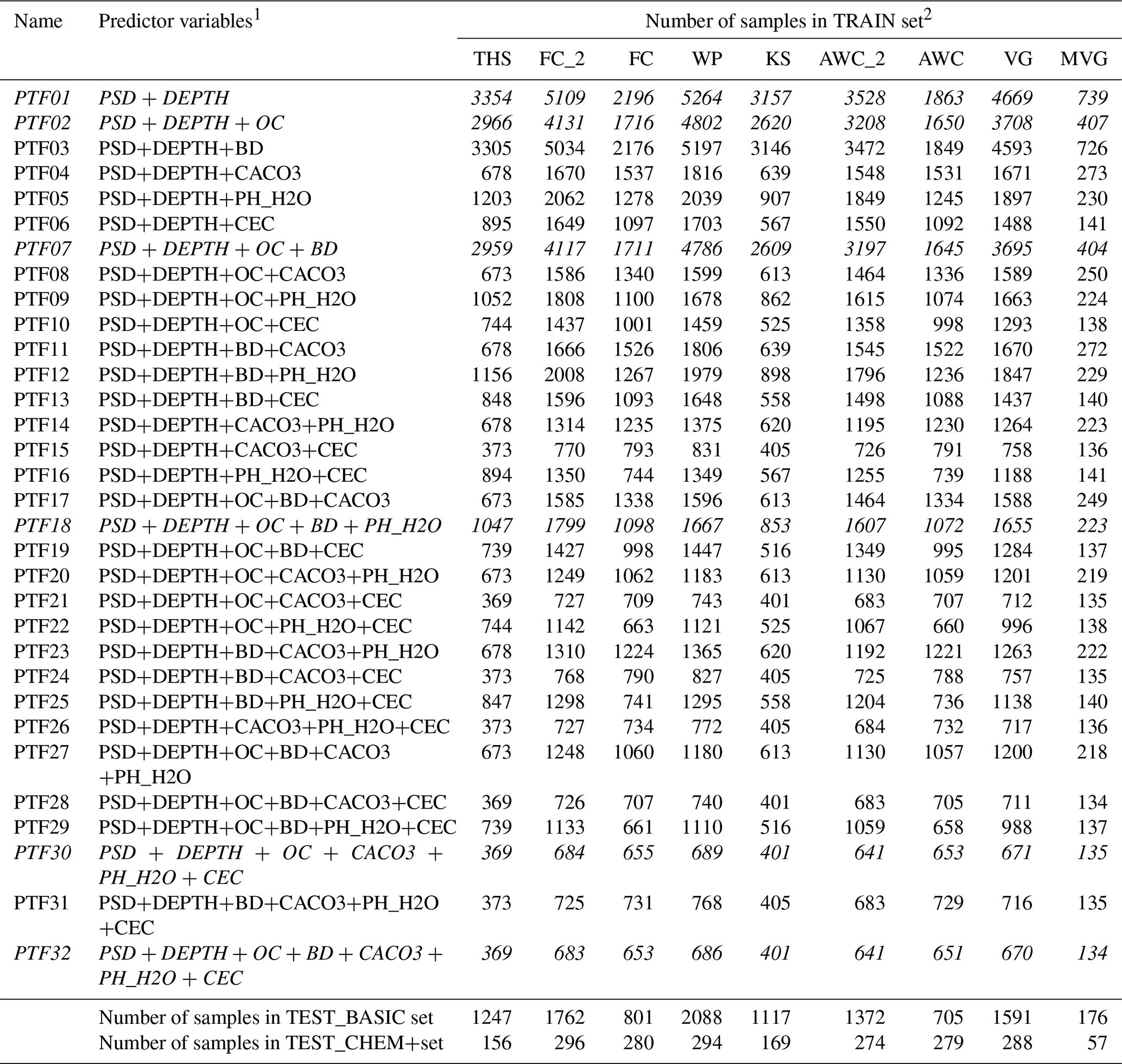
1 PSD: particle size distribution (sand, 50–2000 µm; silt, 2–50 µm; clay, < 2 µm (mass %)); DEPTH: mean soil depth (cm); OC: organic carbon content (mass %); BD: bulk density (g cm−3); CACO3: calcium carbonate content (mass %); PH_H2O: pH in water (–); CEC: cation exchange capacity (cmol (+) kg−1). 2 THS: saturated water content (pF 0); FC_2: water content at −100 cm matric potential head (pF 2.0); FC: water content at −330 cm matric potential head (pF 2.5); AWC_2: plant available water content based on FC_2; AWC: plant available water content based on FC; WP: water content at wilting point (pF 4.2); KS: saturated hydraulic conductivity; VG: parameters of the van Genuchten model; MVG: parameters of the Mualem – van Genuchten model; TEST_BASIC: samples with measured PSD, DEPTH, OC and BD; TEST_CHEM+: samples with measured PSD, DEPTH, OC, BD, CACO3, PH_H2O and CEC.
2.4 The Random Forest algorithm to derive PTFs
We derived the PTFs adopting the random forest method (Breiman, 2001), implemented in the “ranger” R package (Wright and Ziegler, 2017). We selected this method, because (i) it is among the best performing prediction algorithms if there is a complex interaction structure in the dataset (Boulesteix et al., 2012), (ii) it computes quantiles of the predicted values, (iii) parallel processing is supported which saves significant computation time, and (iv) the initially black-box type algorithm can be interpreted based on computing variable importance and analysing partial dependence plots implemented in the “pdp” R package (Greenwell, 2017b).
In the case of a continuous response variable, a random forest is an ensemble of de-correlated regression trees (Breiman, 2001). The regression tree approach divides the predictor space into non-overlapping regions through minimizing the residual sum of squares. The aim of the method is to subset the data as homogeneously as possible at each split. The observations can be assigned to the defined regions in which the mean of the response variable is the predicted value. Single trees of the forest are noisy and limited in performance, but if many unbiased trees are derived and averaged with bagging, the variance is reduced and performance of the prediction improves (Hastie et al., 2009). Building of de-correlated trees is achieved by randomization at two levels. Firstly, each tree of the forest is grown on a randomly selected two thirds of the data with replacement, which is called bootstrap sample or in-bag fraction. Secondly, at each node of a single tree, randomly selected sets of predictors are analysed to split the data. This feature of randomization allows correlation between the response variables (Ziegler and König, 2014), which is an important advantage in the case of pedotransfer functions where predictors are often highly correlated.
Parameter tuning of the ranger was performed with the “caret” R package (Kuhn et al., 2017, 2018). With the implemented train function, a fivefold cross-validation was repeated 10 times to tune the number of randomly selected predictor variables at each split (mtry) and find the best performing splitting rule (splitrule) during training. We started the tuning by setting the number of randomly selected predictor variables to two, then added one by one until the number of all available predictors for each input variable combination was reached. All three built-in splitting rules in the ranger function were tuned, namely variance, extratrees and maxstat. The minimum node size was kept to 10. In addition to the tuning options included in the train function of the caret package, we optimized the number of trees in the forest. The above described tuning was performed by discretely altering the number of trees in the forest in separate tuning steps to 50, 100, 200, 500 and 1000, analysing the results and choosing the best number of trees for the random forest.
We analysed the relevance of predictors and their influence on the response variable. The relevance of predictors was determined by computing the variable importance based on the mean decrease in impurity (Hastie et al., 2009) in the ranger function. The relative importance was assessed by dividing the variable importance of each predictor by the sum of the importance of all the predictors after Kotlar et al. (2019). The marginal effect of some selected predictors on the response – soil hydraulic parameters – was analysed with partial dependence plots (Greenwell, 2017a, b).
The final prediction algorithm was built on the whole training set based on the result of the tuning. To quantify the prediction uncertainties, quantile regression was used (Meinshausen, 2006). In random forest, as implemented in ranger, it is called quantile regression forest. For each node in each tree, the quantile regression forest not only keeps the mean of the predicted target variable, but all observations that belong to that node from which the full conditional distribution of the predicted variable is estimated. The width of the prediction interval varies with the predictor variables. The smaller the range of the prediction interval, the more accurate the prediction is. We analysed the 90 % prediction interval for all predictions, but the derived algorithms (PTFs) provide the possibility to compute the individual predictions of each tree.
2.5 Evaluation of derived PTFs
The performance of the PTFs was calculated using the median values predicted by the random forests. It was described with the root mean square error (RMSE) (Eq. 3.), and the coefficient of determination (R2) (Eq. 4.) computed for the training and test sets.
where yi is the measured and the predicted soil water content or log-transformed saturated or unsaturated hydraulic conductivity, is the average of yi, N is the number of yi and data pairs, and MSE is the mean square error. The different data range of the dataset influences the performance of the PTFs when that is compared to the studies in the literature. Therefore, normalized RMSE (NRMSE) was computed (Eq. 5), where ymax and ymin are the maximum and minimum value of variable.
For each predicted variable, there was an initial set of 32 predictor combinations (Table 1), whose individual performance for each of the predicted variables was assessed. Based on the test results, we derived recommendations which PTF should be used when certain sets of predictor variables are available. We compared the performance of PTFs to quantify if there are significant differences between the predictions as a consequence of adding certain soil properties to the predictor variables. We also compared the performance of point and parameter estimations for those input combinations, which reflect the most frequently available soil property combination from a practical point of view. The aim of this comparison was to analyse whether point or parametric prediction performs better when only THS and/or FC/FC_2 and/or WP are needed.

Figure 1Results of parameter tuning of the random forest: optimization of (a) the number of randomly selected predictors at each split by number of available predictors and (b) splitting rule applied to build the trees in the random forest.
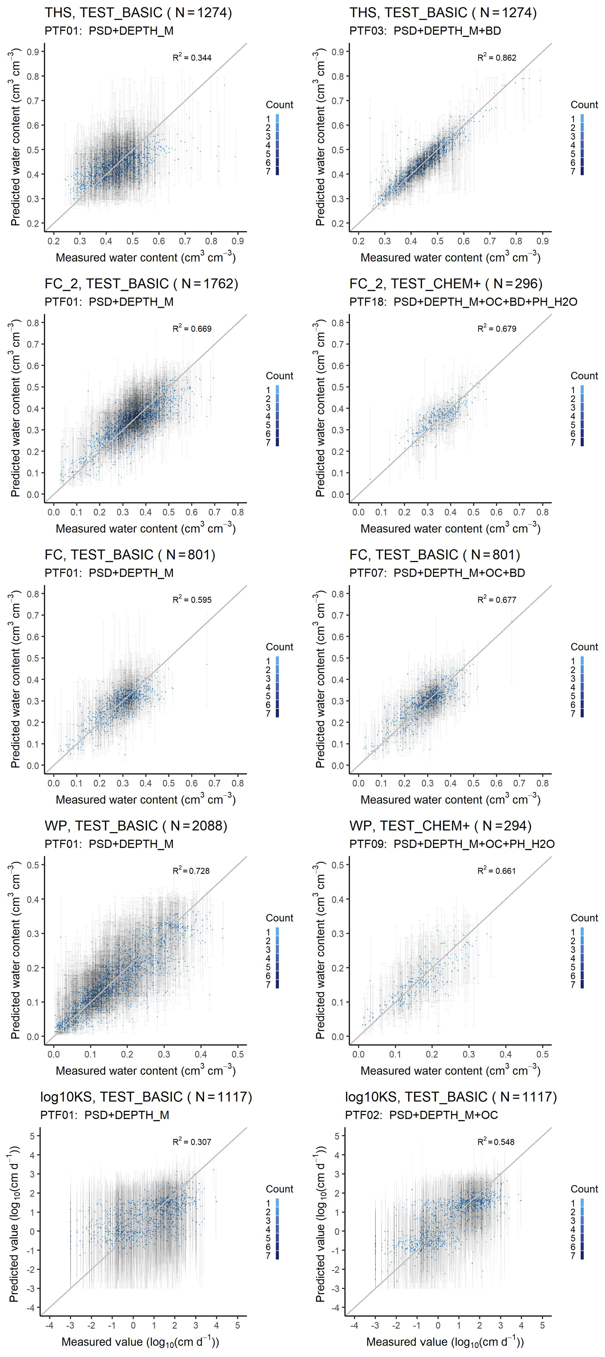
Figure 2Scatter plot of the measured versus median predicted water retention values of the worst and best performing PTF with 90 % prediction interval on test datasets. THS: saturated water content (PTF01 vs. PTF03); FC_2: water content at −100 cm matric potential head (PTF01 vs. PTF18); FC: water content at −330 cm matric potential head (PTF01 vs. PTF07); WP: water content at wilting point (PTF01 vs. PTF09); log10KS: saturated hydraulic conductivity (PTF01 vs. PTF02); PSD: particle size distribution (sand, 50–2000 µm; silt, 2–50 µm; clay, < 2 µm (mass %)); DEPTH_M: mean soil depth (cm); OC: organic carbon content (mass %); BD: bulk density (g cm−3); PH_H2O: pH in water (–); Count: the number of cases in each rectangle.
Additionally, the performance of the presented random forest based PTFs was compared to that of the euptfv1 (Tóth et al., 2015). For comparison, those PTFs from euptfv2 were selected which corresponded to the analysed input variable combination of the euptfv1.
The comparison of PTFs was done using a non-parametric Kruskal-Wallis test at the 5 % significance level applied on the MSE values – computed on TEST_BASIC and/or TEST_CHEM+ sets (Table 1) – using the R package agricolae (De Mendiburu, 2017). Recommendation of PTFs for a given set of predictor variables was based on the performance of euptfv2 on the test sets. If there was no significant difference in performance, the PTF derived from the largest population was selected.
All statistical analysis was performed in R [version 3.6.0] (R Core Team, 2019).
3.1 General performance
In the process of tuning the random forest parameters, the number of trees was found to be sufficient when set to 200 in all cases. The number of candidate predictors was found to be higher than the recommended square root of the number of available predictor variables (p) in most of the cases, especially when p was greater than 5 (Fig. 1). When optimizing the splitting rules to build the trees in the forest, overall, the best performance was achieved by the extratrees rule in 54 %, by the variance rule in 28 %, and by the maxstat rule in 18 % of the cases (Fig. 1).
The RMSE values were between 0.020 and 0.068 cm3 cm−3 for THS (Table 2), 0.046 and 0.055 cm3 cm−3 for FC (Table 3), 0.040 and 0.060 cm3 cm−3 for FC_2 (Table 4), 0.037 and 0.048 cm3 cm−3 for WP (Table 5), 0.043 and 0.053 cm3 cm−3 for AWC (Table S1 in the Supplement), 0.045 and 0.060 cm3 cm−3 for AWC_2 (Table S2), and 0.09 and 1.18 log10 (cm d−1) for KS (Table 6) in the case of including different predictor variables computed on the test sets. Table S3 shows the NRMSE for the point predictions computed for the TEST_BASIC and TEST_CHEM+ sets to provide possibility for comparison with other PTFs available from the literature. In the case of VG and MVG, RMSE for the entire matric potential head range was between 0.041 and 0.068 cm3 cm−3 for the moisture retention (Table 7) and 0.61 and 0.71 log10 (cm d−1) for the hydraulic conductivity (Table 8). These RMSE values are within the range of recently published PTFs (McNeill et al., 2018; Nguyen et al., 2017; Román Dobarco et al., 2019; Zhang and Schaap, 2017).
In the case of the point estimations, Figs. 2, S1 depict the scatterplots of measured and predicted soil hydraulic properties/parameters with 90 % prediction interval computed on the test sets. Performance of the worst to best PTFs are shown. The addition of predictors that significantly improve the predictions also decreases the uncertainty. The largest reduction in the width of the inner 90 % of the prediction interval is visible for THS. Specifically this value decreased from 0.21 to 0.10 cm3 cm−3 for THS, from 0.19 to 0.14 cm3 cm−3 for FC_2, from 0.17 to 0.14 cm3 cm−3 for FC, from 0.15 to 0.14 cm3 cm−3 for WP, from 0.19 to 0.17 cm3 cm−3 for AWC_2, from 4.1 to 3.2 log10 (cm d−1) for KS. In the case of AWC the mean 90 % mean interval did not change (0.15 cm3 cm−3).
Figures S2, S4, S6, S8, S10, S12, S14, S16, S19 show the squared error of the derived PTFs computed on the TEST_BASIC and TEST_CHEM+ sets. The PTFs are ordered based on their performance. Density plots of measured and predicted soil hydraulic values are included in Figs. S3, S5, S7, S9, S11, S13, S15, S17, S20. Plots show the PTFs that use the most frequently available predictors.
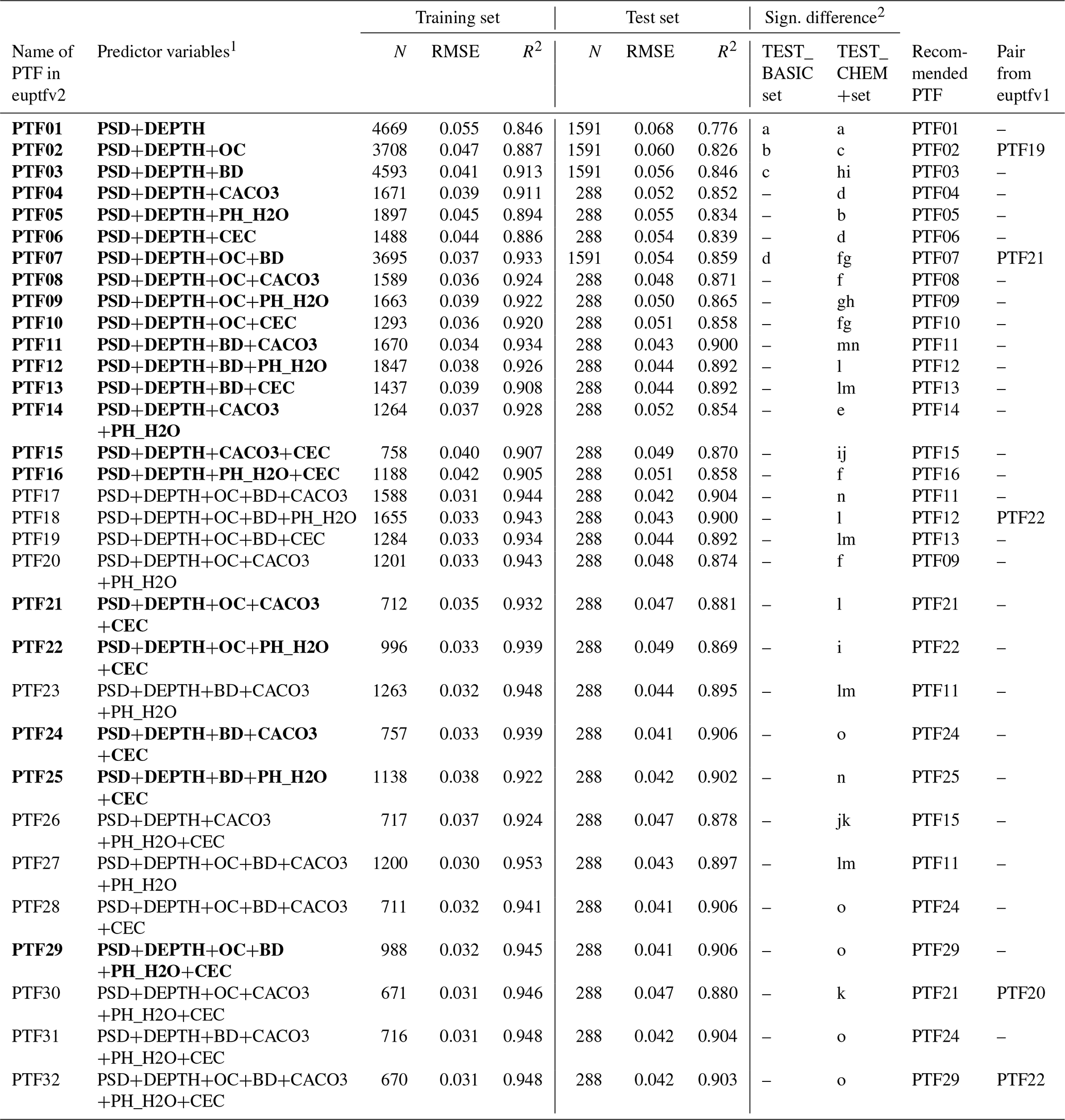
Table 2Performance of pedotransfer functions (PTFs) by input combination on training and test datasets to predict water content at saturation (THS). N: number of samples, RMSE: root mean square error (cm3 cm−3), and R2: determination coefficient, TEST_BASIC: samples with measured PSD, DEPTH, OC and BD; TEST_CHEM+: samples with measured PSD, DEPTH, OC, BD, CACO3, PH_H2O and CEC. Recommended PTFs are highlighted in bold.
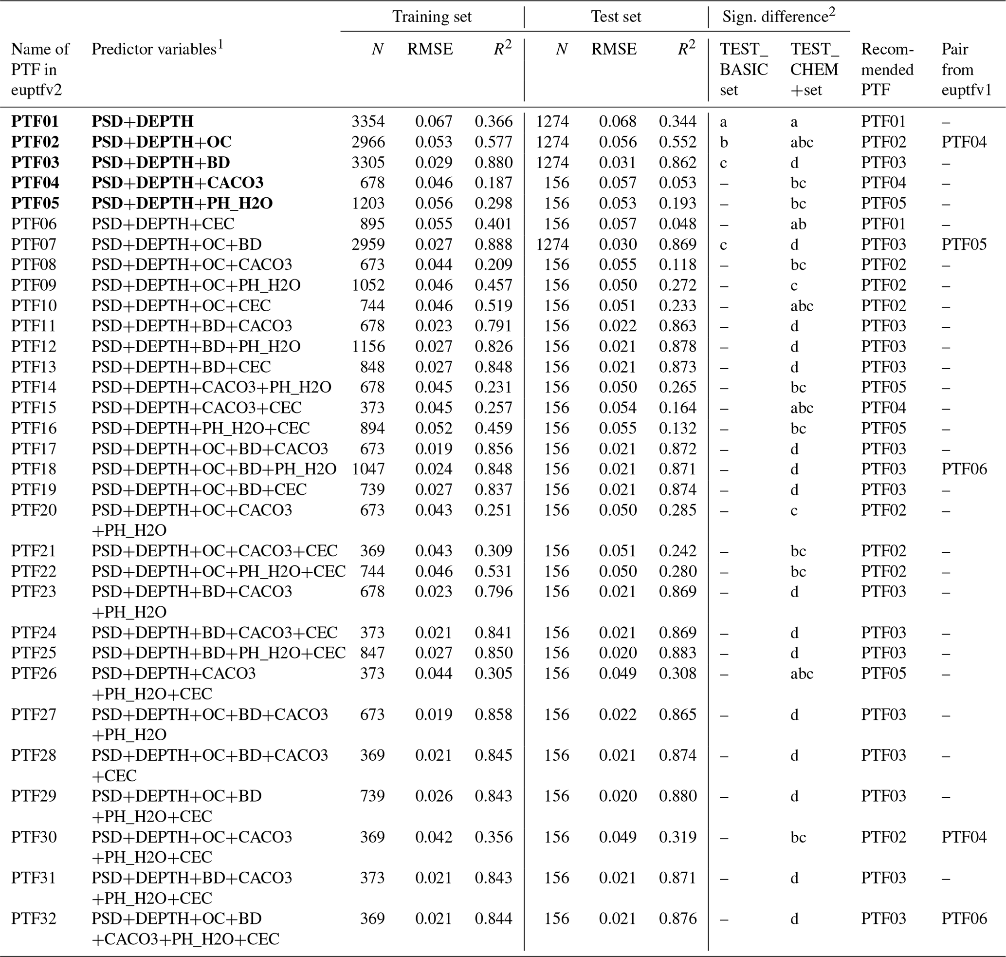
1 PSD: particle size distribution (sand, 50–2000 µm; silt, 2–50 µm; clay, <2 µm (mass %)); DEPTH: mean soil depth (cm); OC: organic carbon content (mass %); BD: bulk density (g cm−3); CACO3: calcium carbonate content (mass %); PH_H2O: pH in water (–); CEC: cation exchange capacity (cmol (+) kg−1). 2 Different letters indicate significant differences at the 0.05 level between the accuracy of the methods based on the squared error; for example performance indicated with the letter c is significantly better than the one noted with letters b and a.
Table 3Performance of pedotransfer functions (PTFs) by input combination on training and test datasets to predict water content at −100 cm matric potential head (FC_2). N: number of samples, RMSE: root mean square error (cm3 cm−3), and R2: determination coefficient, TEST_BASIC: samples with measured PSD, DEPTH, OC and BD; TEST_CHEM+: samples with measured PSD, DEPTH, OC, BD, CACO3, PH_H2O and CEC. Recommended PTFs are highlighted in bold. FC_2 was not analysed in euptfv1.

1 PSD: particle size distribution (sand, 50–2000 µm; silt, 2–50 µm; clay, < 2 µm (mass %)); DEPTH: mean soil depth (cm); OC: organic carbon content (mass %); BD: bulk density (g cm−3); CACO3: calcium carbonate content (mass %); PH_H2O: pH in water (–); CEC: cation exchange capacity (cmol (+) kg−1). 2 Different letters indicate significant differences at the 0.05 level between the accuracy of the methods based on the squared error; for example performance indicated with the letter c is significantly better than the one noted with letters b and a.
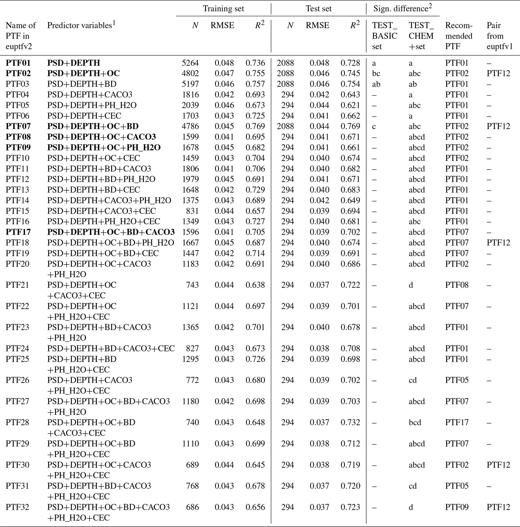
Table 4Performance of pedotransfer functions (PTFs) by input combination on training and test datasets to predict water content at −330 cm matric potential head, field capacity (FC). N: number of samples, RMSE: root mean square error (cm3 cm−3), and R2: determination coefficient, TEST_BASIC: samples with measured PSD, DEPTH, OC and BD; TEST_CHEM+: samples with measured PSD, DEPTH, OC, BD, CACO3, PH_H2O and CEC. Recommended PTFs are highlighted in bold.

1 PSD: particle size distribution (sand, 50–2000 µm; silt, 2–50 µm; clay, < 2 µm (mass %)); DEPTH: mean soil depth (cm); OC: organic carbon content (mass %); BD: bulk density (g cm−3); CACO3: calcium carbonate content (mass %); PH_H2O: pH in water (–); CEC: cation exchange capacity (cmol (+) kg−1). 2 Different letters indicate significant differences at the 0.05 level between the accuracy of the methods based on the squared error; for example performance indicated with the letter c is significantly better than the one noted with letters b and a.
Table 5Performance of pedotransfer functions (PTFs) by input combination on training and test datasets to predict water content at wilting point (WP). N: number of samples, RMSE: root mean square error (cm3 cm−3), and R2: determination coefficient, TEST_BASIC: samples with measured PSD, DEPTH, OC and BD; TEST_CHEM+: samples with measured PSD, DEPTH, OC, BD, CACO3, PH_H2O and CEC. Recommended PTFs are highlighted in bold.
1 PSD: particle size distribution (sand, 50–2000 µm; silt, 2–50 µm; clay, < 2 µm (mass %)); DEPTH: mean soil depth (cm); OC: organic carbon content (mass %); BD: bulk density (g cm−3); CACO3: calcium carbonate content (mass %); PH_H2O: pH in water (–); CEC: cation exchange capacity (cmol (+) kg−1). 2 Different letters indicate significant differences at the 0.05 level between the accuracy of the methods based on the squared error; for example performance indicated with the letter c is significantly better than the one noted with letters b and a.
This study strengthens the importance of chemical soil properties in the prediction. CEC was found to be an important predictor by Pachepsky and Rawls (1999) for FC and WP, by Botula et al. (2013) for water retention at several matric potential head values, and by Hodnett and Tomasella (2002) for the VG parameters. Hodnett and Tomasella (2002) showed that pH influenced all four VG parameters. The role of CACO3 was shown to be not significant in the study of Khodaverdiloo et al. (2011). They highlight that a possible influence of CACO3 might already have been indirectly included by bulk density. The role of PSD, BD and OC has been studied extensively by various authors, e.g. Nemes et al. (2003), Rawls et al. (2003), Vereecken et al. (1989), Weynants et al. (2009), Wösten et al. (1999), which is in line with the general pattern of variable influence we see in this study.
Table S3 summarizes the recommended PTF for each combination of available predictor variables. The importance and influence of soil properties on the performance of hydraulic PTFs and results of partial dependence plots are reported below by predicted soil hydraulic properties.
3.2 Point estimations
The performance of the PTFs was computed for the training and test sets (Tables 2–8 and S1–2) indicating the presence of significant differences. For each predictor variable, the recommended PTF number is indicated and its predictor variables are highlighted in bold font in the respective tables. For easier comparison with euptfv1, the corresponding PTF number used in Tóth et al. (2015) is additionally provided in each table. In the following, detailed results of the constructed PTFs for the individual predicted variables are presented and discussed.
3.2.1 Water content at saturation
Table 2, Figs. S2 and S3 show the performance of the PTFs predicting THS. The best performing random forest is PTF03. It is also the one trained on the largest population. It uses PSD, DEPTH and BD as predictors. For the prediction of THS, the most important variable by far is BD (Fig. 3). When BD is not used for the computation of THS, values above 0.60 cm3 cm−3 are not well predicted (Fig. S3). The addition of OC or CACO3 or PH_H2O to PSD and DEPTH improves significantly the performance of the PTF. The picture changes if BD is known: if PSD, DEPTH and BD were available, further addition of OC or CACO3 or PH_H2O or CEC does not significantly improve the prediction, neither do their combinations. Figure 4 shows the dependence of THS on OC and BD, considering the average effect of the other predictor variables – i.e. PSD and DEPTH. When BD is lower than 1.5 g cm−3 changes in OC do not influence THS. If BD is larger than 1.5 g cm−3, samples with higher OC have higher THS.
3.2.2 Water content at field capacity
The performance of the PTFs computed on training and test set are shown in Table 3, Figs. S4 and S5 for FC_2 and in Table 4, Figs. S6 and S7 for FC. The best performing PTF derived from the largest population is the one using (i) PSD, DEPTH, OC, BD and PH_H2O (PTF18) in the case of FC_2, and (ii) PSD, DEPTH, OC and BD (PTF07) for FC.
For FC_2, the two most important variables are USSAND and BD (Fig. 3). When BD and USSAND increase, FC_2 decreases (Fig. 4). Adding OC or BD to PSD and DEPTH significantly improves the prediction of FC_2. If either of CACO3, PH_H2O or CEC is added as a further predictor to PSD and DEPTH, the performance of the PTF does not significantly improve. If PSD, DEPTH and BD are available, adding OC or CACO3 or PH_H2O does not significantly improve the prediction. Including CEC as an additional predictor besides PSD, DEPTH and BD, significantly improves the estimation of FC_2.
USSAND and USCLAY are the two most important variables for the prediction of FC (Fig. 3). Instead of analysing these two soil properties, both characterizing the soil texture, we include OC next to USSAND in the partial dependence plot analysis, because the amount of OC can be altered due to change in climate, land use, soil and water management, cropping systems, etc. (Wiesmeier et al., 2019). Within the range of OC in the dataset FC increases with increasing OC regardless of USSAND content by up to 0.08 cm3 cm−3 even when USSAND is greater than 60 % (Fig. 4). Adding OC or CEC to PSD and DEPTH significantly improves the prediction of FC. The effect of CEC on the prediction of FC was also shown by Pachepsky and Rawls (1999). BD or CaCO3 or PH_H2O do not significantly improve the predictions if PSD, DEPTH, or PSD, DEPTH and OC are available. Predictions significantly improve when both CaCO3 and PH_H2O are added as predictors to PSD, DEPTH and OC.
3.2.3 Water content at wilting point
The performance of PTFs derived for WP prediction is shown in Table 5, Figs. S8 and S9. Among the best performing PTFs, PTF09 is derived on the largest training set. It uses PSD, DEPTH, OC and PH_H2O as predictors. Even though the most important variables for WP prediction were USCLAY and USSAND (Fig. 3), we included OC on the partial dependence plot (Fig. 4) as in the FC analysis. USCLAY had the strongest influence on WP. The influence of OC on WP can be detected for soils with OC less than 4 % and USCLAY less than 50 %. Below 10 % USCLAY, the WP slightly increases with increasing OC. When USCLAY is between 10 % and 50 % and OC is less than 4 %, increasing OC generally decreases WP.
OC significantly improves the prediction of WP if added to PSD and DEPTH. If BD or CACO3 or PH_H2O or CEC are added to PSD and DEPTH, the performance of the prediction does not improve significantly. Adding CACO3 and CEC to PSD, DEPTH and OC significantly improves the prediction.
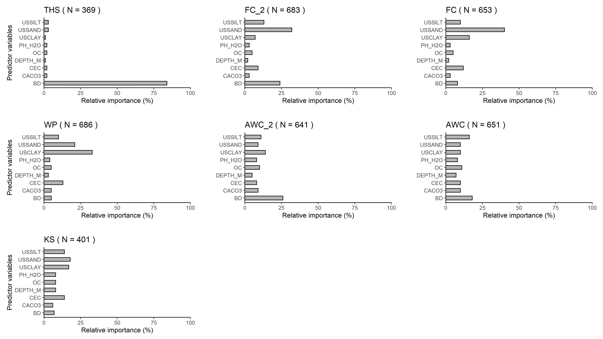
Figure 3Relative variable importance computed with the random forest algorithm for the prediction of water content with PTF32 at saturation (THS), at field capacity; −100 (FC_2) and −330 (FC) matric potential head, at wilting point (WP), of the plant available water content based on FC_2 (AWC_2) and FC (AWC), and the saturated hydraulic conductivity (KS). USSILT: silt content (2–50 µm (mass %)); USSAND: sand content (50–2000 µm (mass %)); USCLAY: clay content (< 2 µm (mass %)); PH_H2O: pH in water (–); OC: organic carbon content (mass %); DEPTH_M: mean soil depth (cm); OC: organic carbon content (mass %); CEC: cation exchange capacity (cmol (+) kg−1); CACO3: calcium carbonate content (mass %); BD: bulk density (g cm−3).
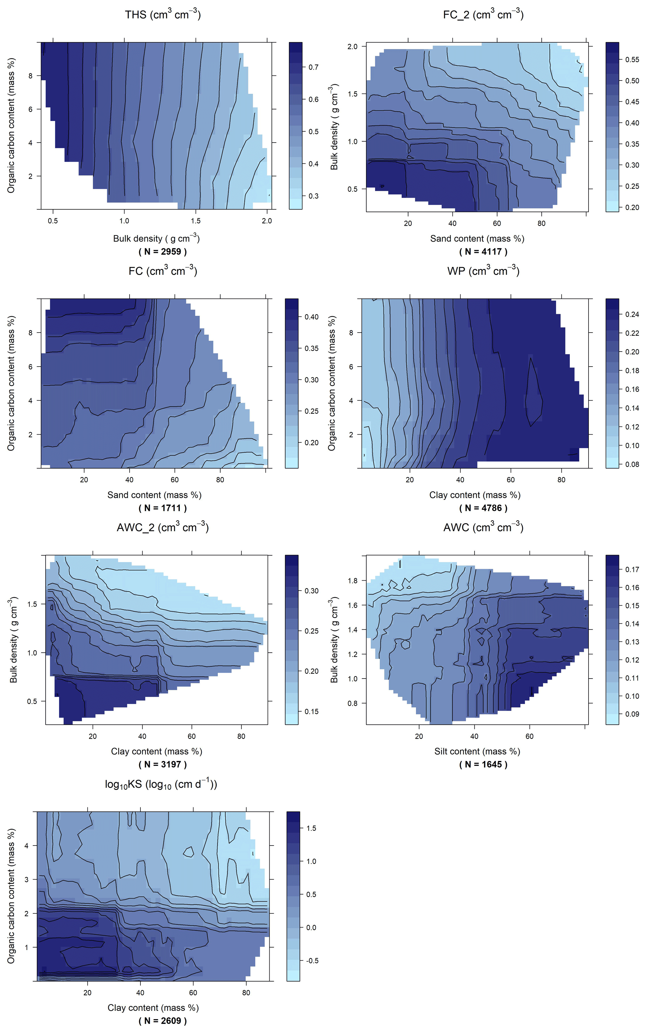
Figure 4Partial dependence plot computed based on the random forest algorithm (PTF07) for the prediction of water content at saturation (THS), field capacity at −100 (FC_2) and −330 (FC) matric potential head, wilting point (WP), plant available water content computed with field capacity at −100 and −330 cm matric potential head (AWC_2, AWC) and saturated hydraulic conductivity (KS) for selected predictors.
3.2.4 Plant available water content
Tables S1, S2 and Figs. S1, S10–13 show the performance of AWC and AWC_2 predictions. Considering PSD, DEPTH, and BD as input, PTF03 is the best performing algorithm and in both case had the largest training data sets. For both AWC and AWC_2, BD is the most important predictor among the analysed variables (Fig. 3). The second most important variable is USCLAY in the case of AWC_2 and USSILT for AWC. Increasing BD and USCLAY decreases AWC_2. In the case of AWC, increasing BD and decreasing USSILT decreases the water content (Fig. 4).
OC and BD significantly improve the prediction of AWC_2 when added as input variables next to PSD and DEPTH. If either BD or OC is already included, adding the respective other, does not significantly improve the prediction. Neither PH_H2O, CACO3 nor CEC improves the prediction.
For the prediction of AWC, further addition of only BD or OC or CACO3 or PH_H2O or CEC to PSD and DEPTH does not significantly improve the prediction. If both OC and BD are included as predictors next to PSD and DEPTH, the prediction significantly improves.
There is no significant difference between direct and indirect predictions, neither for AWC nor for AWC_2. However, the size of the test set used for the statistical analysis is limited. There were only 145 samples in the TEST_BASIC set and 64 samples in TEST_CHEM+ set after merging datasets available for both direct and indirect predictions for analysing AWC, and 70 and 34 samples in the case of AWC_2. Thus, if prediction of FC_2/FC and WP are needed in addition to AWC_2/AWC, we recommend computing AWC from those to save on computing time. Variation in AWC could be explained less efficiently (Tables S1, S2) than the other studied water retention values but the performance of the prediction is comparable with that of published values in the literature (Li et al., 2016; Malone et al., 2009).
Table 6Performance of pedotransfer functions (PTFs) by input combination on training and test datasets to predict saturated hydraulic conductivity (KS). N: number of samples, RMSE: root mean square error (log10 (cm d−1)), and R2: determination coefficient, TEST_BASIC: samples with measured PSD, DEPTH, OC and BD; TEST_CHEM+: samples with measured PSD, DEPTH, OC, BD, CACO3, PH_H2O and CEC. Recommended PTFs are highlighted in bold.

1 PSD: particle size distribution (sand, 50–2000 µm; silt, 2–50 µm; clay, < 2 µm (mass %)); DEPTH: mean soil depth (cm); OC: organic carbon content (mass %); BD: bulk density (g cm−3); CACO3: calcium carbonate content (mass %); PH_H2O: pH in water (–); CEC: cation exchange capacity (cmol (+) kg−1). 2 Different letters indicate significant differences at the 0.05 level between the accuracy of the methods based on the squared error; for example performance indicated with the letter c is significantly better than the one noted with letters b and a.

Figure 5Scatter plot of the measured versus median predicted water retention values computed with the van Genuchten (VG) model (PTF01 vs. PTF29, i.e. the worst versus best performing PTF). PSD: particle size distribution (sand, 50–2000 µm; silt, 2–50 µm; clay, < 2 µm (mass %)); DEPTH_M: mean soil depth (cm); OC: organic carbon content (mass %); BD: bulk density (g cm−3); PH_H2O: pH in water (–); CEC: cation exchange capacity (cmol (+) kg−1); Count: the number of cases in each hexagon.
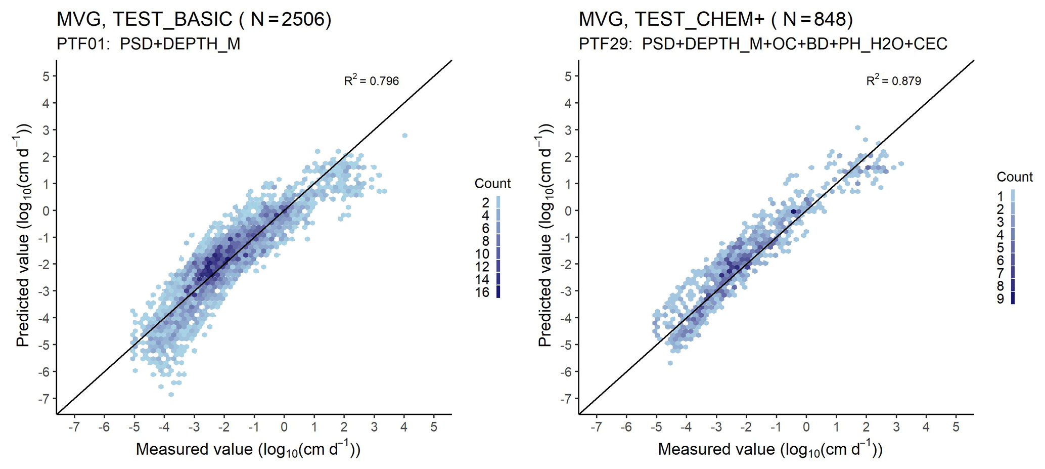
Figure 6Scatter plot of the measured versus median predicted hydraulic conductivity values computed with the Mualem–van Genuchten (MVG) model (PTF01 vs. PTF27, i.e. the worst versus best performing PTF). PSD: particle size distribution (sand, 50–2000 µm; silt, 2–50 µm; clay, < 2 µm (mass %)); DEPTH_M: mean soil depth (cm); OC: organic carbon content (mass %); BD: bulk density (g cm−3); CACO3: calcium carbonate content (mass %); PH_H2O: pH in water (–); Count: the number of cases in each hexagon.
3.2.5 Saturated hydraulic conductivity
The performance of KS prediction is shown in Table 6, Figs. S14 and S15. The predictors of the best performing PTF derived on the largest training set are PSD, DEPTH and OC (PTF02). The prediction of KS significantly improves if OC is included among the predictor variables next to PSD and DEPTH. No other predictors significantly improve the performance of the PTF. On the training dataset, when OC is greater than 2.5 %, the influence of clay content on KS is more dominant than that of OC (Fig. 4). In the case of KS prediction, the simplest best performing PTF – which was derived on a training dataset with KS ranging between −3.00 and 4.67 log10 (cm d−1) – has an RMSE of 0.94 log10 (cm d−1) and NRMSE 0.14 log10 (cm d−1) (Table S3). PSD and CEC are the most important input variables for the prediction of KS when all nine variables are considered as predictors (Fig. 3). In that case, OC is the fifth and BD is only the eighth most important variable. The prediction performance is influenced by the heterogeneity of measurement methods of KS in the EU-HYDI dataset. When the methods are homogeneous, the RMSE value is usually around 0.6–0.8 log10 (cm d−1) as reviewed by Zhang and Schaap (2019). ROSETTA3 PTF with PSD and BD predictors had an RMSE of 0.68 log10 (cm d−1) with an NRMSE of 0.11 log10 (cm d−1) (Zhang and Schaap, 2017). Araya and Ghezzehei (2019) published PTF using PSD, BD and OC predictors with the highest accuracy in the literature with an RMSE of 0.34 log10 (cm d−1) and NRMSE of 0.06 log10 (cm d−1). In Lilly et al. (2008), the performance of the KS predictions and findings were similar to this study. They report an RMSE between 0.95 and 1.08 log10 (cm d−1) – with an NRMSE between 0.17 and 0.20 log10 (cm d−1) – for the KS prediction when analysed with several input combinations. Even when information on soil structure and crack orientation was considered – next to topsoil and subsoil distinction, PSD, BD and OC – the RMSE was 0.97 log10 (cm d−1). BD would be among the most important variables, but also in their analysis its influence was masked out. They derived the PTFs on the HYPRES dataset (Wösten et al., 1999), which also includes very diverse methods to determine the saturated hydraulic conductivity and part of which is also contained in the EU-HYDI. The uncertainty in the predictions (Fig. 2) could be decreased if the predictions would be differentiated according to the measurement methods, but that might decrease the applicability of the PTFs. On the contrary, this study indicates the necessity to include saturated hydraulic conductivity values determined from many different measurement techniques, otherwise, the PTFs are expected to lose their generality.
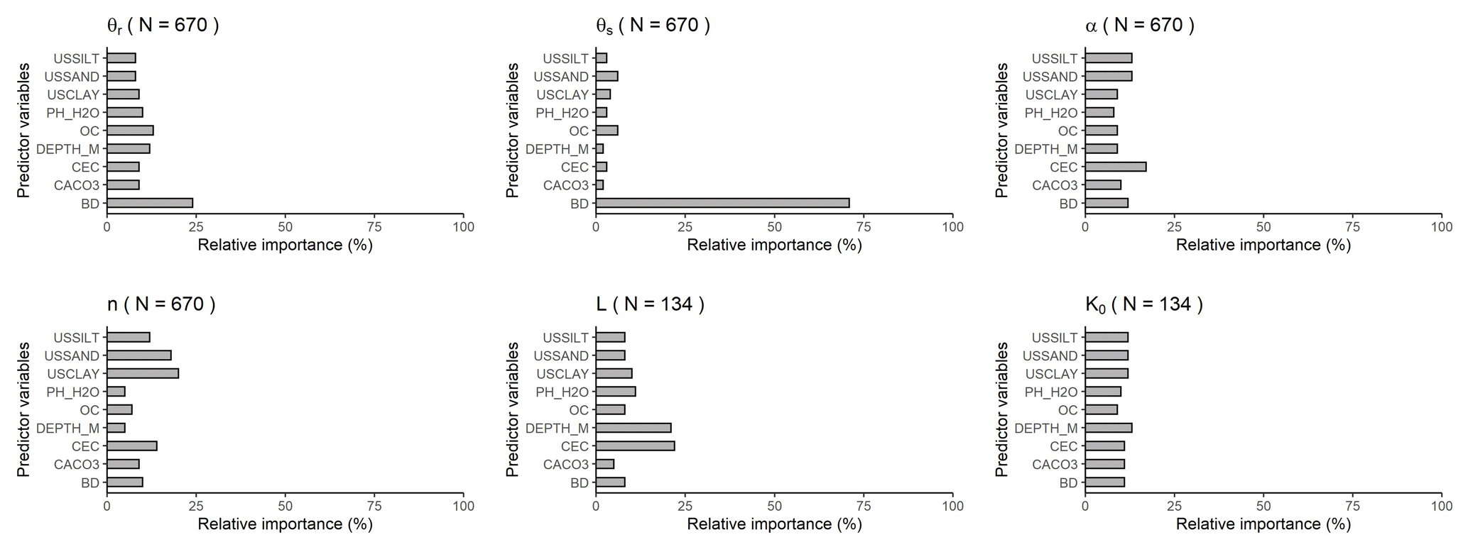
Figure 7Relative variable importance computed with the random forest algorithm for the prediction of parameters of the van Genuchten and Mualem–van Genuchten models based on PTF32. θr: residual water content (cm3 cm−3); θs: saturated water content (cm3 cm−3); α (cm−1), n (–): shape parameters; K0: the hydraulic conductivity acting as a matching point at saturation (cm d−1); L: shape parameter related to pore tortuosity (–); USSILT: silt content (2–50 µm (mass %)); USSAND: sand content (50–2000 µm (mass %)); USCLAY: clay content (< 2 µm (mass %)); PH_H2O: pH in water (–); OC: organic carbon content (mass %); DEPTH_M: mean soil depth (cm); OC: organic carbon content (mass %); CEC: cation exchange capacity (cmol (+) kg−1); > CACO3: calcium carbonate content (mass %); BD: bulk density (g cm−3).
3.3 Parameter estimations
The performance of parametric PTFs are shown in Tables 7 and 8 and Figs. 5, 6, S16–S21. Figure 7 illustrates the importance of variables for the prediction of VG and MVG parameters. The best performing PTF derived on the largest training set is PTF29 – with PSD, DEPTH, OC, BD, PH_H2O and CEC – for MRC and PTF27 – with PSD, DEPTH, OC, BD, CACO3, PH_H2O – for HCC.
For θr, overall, BD is the most important predictor while all other predictors show similar variable importance (Fig. 7). Interpretation of this parameter is complex, but it was demonstrated that it is influenced by the soil specific surface area (Assouline and Or, 2013), and the measured data range (Weber et al., 2019). For θs, the most important predictor is by far BD, similarly to THS. The importance of CEC has to be noted for the prediction of parameters α, n and L. For the prediction of parameter n – which relates to the pore size distribution – USCLAY and USSAND are the most important variables. K0 is influenced by several soil properties besides those included in the dataset used here, e.g. pore connectivity, tortuosity, primary pore orientation. These properties cannot be directly inferred from other soil properties limiting the explanatory power of the available properties. The prediction of K0 remains complex and challenging. Variable importance of all studied predictors is greater than 70 %. Moreover, K0 is influenced by the data quality, and is correlated in parameter space, which is not treated here.
Only a few studies have analysed the importance of CEC for MRC and HCC PTFs (Botula et al., 2013; Hodnett and Tomasella, 2002; Pachepsky and Rawls, 1999) which might be linked to the fact that CEC is rarely available in soil hydraulic datasets. It is noteworthy to highlight that all best performing MRC PTFs (PTF24, PTF28, PTF29, PTF30, PTF31) include CEC among the predictors (Table 7). In addition to that, Hodnett and Tomasella (2002) found that CEC was important for the prediction of θr and α parameters of the van Genuchten model. This is because CEC provides indirect information on soil mineralogy and reflects soil specific surface area, charge density and pore size which influence soil water retention (Lal and Shukla, 2004).
Table 7Performance of pedotransfer functions (PTFs) by input combination on training and test datasets to predict parameters of the van Genuchten model to describe soil moisture retention curve (VG). N: number of samples, RMSE: root mean square error (cm3 cm−3), and R2: determination coefficient, TEST_BASIC: samples with measured PSD, DEPTH, OC and BD; TEST_CHEM+: samples with measured PSD, DEPTH, OC, BD, CACO3, PH_H2O and CEC. Recommended PTFs are highlighted in bold.
1 PSD: particle size distribution (sand, 50–2000 µm; silt, 2–50 µm; clay, < 2 µm (mass %)); DEPTH: mean soil depth (cm); OC: organic carbon content (mass %); BD: bulk density (g cm−3); CACO3: calcium carbonate content (mass %); PH_H2O: pH in water (–); CEC: cation exchange capacity (cmol (+) kg−1). 2 Different letters indicate significant differences at the 0.05 level between the accuracy of the methods based on the squared error; for example performance indicated with the letter c is significantly better than the one noted with letters b and a.
Table 8Performance of pedotransfer functions (PTFs) by input combination on training and test datasets to predict parameters of the Mualem–van Genuchten model to describe soil moisture retention and hydraulic conductivity curve (MVG). N: number of samples, RMSE: root mean square error (log10 (cm d−1)), and R2: determination coefficient, TEST_BASIC: samples with measured PSD, DEPTH, OC and BD; TEST_CHEM+: samples with measured PSD, DEPTH, OC, BD, CACO3, PH_H2O and CEC. Recommended PTFs are highlighted in bold.
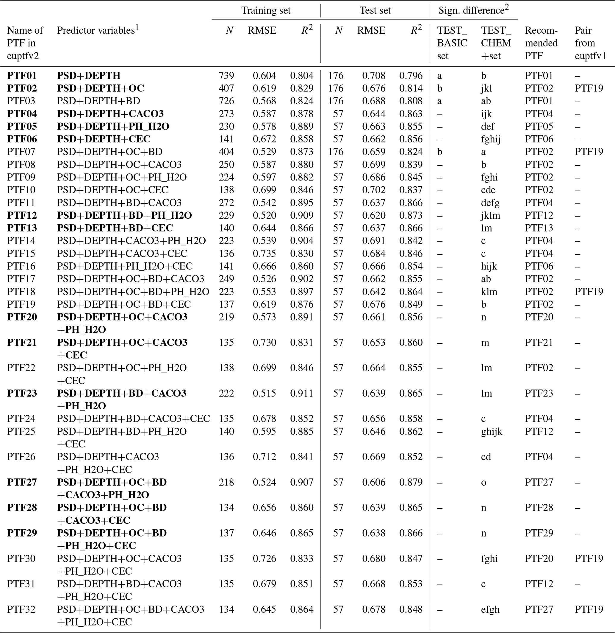
1 PSD: particle size distribution (sand, 50–2000 µm; silt, 2–50 µm; clay, < 2 µm (mass %)); DEPTH: mean soil depth (cm); OC: organic carbon content (mass %); BD: bulk density (g cm−3); CACO3: calcium carbonate content (mass %); PH_H2O: pH in water (–); CEC: cation exchange capacity (cmol (+) kg−1). 2 Different letters indicate significant differences at the 0.05 level between the accuracy of the methods based on the squared error; for example performance indicated with the letter c is significantly better than the one noted with letters b and a.
3.3.1 Moisture retention curve
If BD or OC or CACO3 or CEC or PH_H2O are added as a predictor to information on PSD and DEPTH, the performance of the PTF significantly improves (Table 7, Fig. S16). Adding BD next to PSD and DEPTH improves the predictions more than adding OC (Table 7, Fig. S17). BD and OC together significantly improve the prediction compared to using PSD, DEPTH together with either BD or OC. Adding OC next to PSD, DEPTH, BD and chemical soil properties (CACO3 and/or CEC and /or PH_H2O) does not significantly improve the prediction. If PSD, DEPTH, CACO3 and CEC are available, further addition of PH_H2O does not improve the prediction. The best performing PTF includes USSAND, USSILT, USCLAY, DEPTH, BD, CACO3, CEC. Figure 5 shows a scatterplot of measured and predicted water content values, including the performance of the worst and the best performing PTF (PTF01 and PTF29). The importance of including chemical properties and most importantly bulk density among the predictors is visible when measured water contents are greater than 0.50 cm3 cm−3. Those high water content values are characteristic when the soil is close to saturation, thus indirect information about the structure is needed for more accurate predictions of those water content values. Parametric PTFs underestimate water content near saturation and between −200 and −15 000 cm matric potential head (Fig. S18). Overestimation occurs between −10 and −50 cm matric potential head and above 16 000 cm matric potential head. When chemical soil properties are included, the degree of underestimation decreases between −200 and −15 000 cm matric potential head, but overestimation increases between −5 and −10 cm with around 0.02 cm3 cm−3.
3.3.2 Hydraulic conductivity curve
OC, CACO3, PH_H2O and CEC significantly improves the prediction of HCC when added to PSD and DEPTH. Adding BD next to PSD and DEPTH does not improve the predictions (Table 8, Figs. S19, S20). If PSD, DEPTH and OC are used as predictors, further addition of BD or CACO3 or PH_H2O or CEC does not significantly improve the performance of the PTFs. However, adding CaCO3 and CEC or PH_H2O significantly improve the prediction. The performance of the worst and the best performing PTF is shown on Fig. 6. The PTF with only PSD and DEPTH underestimate hydraulic conductivity values smaller than 0.01 cm d−1. When OC, BD, PH_H2O and CEC are included, the underestimation decreases. This could be explained by the fact that these predictors contain indirect information on soil particle surface area and surface characteristics, which are some of the governing properties of low hydraulic conductivities.
When soil chemical properties are not used as predictors, hydraulic conductivity is underestimated close to saturation and at matric potential heads smaller than −500 cm; overestimation occurs between −10 and −500 cm matric potential head (Fig. S21). If chemical properties are also considered, hydraulic conductivity is (i) underestimated at matric potential head smaller than −5000 cm, and (ii) overestimated between −5 and −5000 cm. With added information on chemical properties, the degree of underprediction decreases close to saturation and at the very dry end of the hydraulic conductivity curve. An increase in prediction performance for values lower than 0.1 cm d−1 is visible also on Fig. 6.
Samples with measurements of the HCC at pressure heads cm are less frequent and are not as numerous within a dataset of a single sample, if it was measured. Since the dataset of estimated VG model parameters was identical in this study and in Tóth et al. (2015), differences between the two studies of the unsaturated HCC are related to the PTF methods involved. However, at pressure heads cm, the HCC is dominated by non-capillary conductivity (Streck and Weber, 2020; Weber et al., 2019), which is not included in the MVG model. The considerable data mismatch observable for the dry range (Fig. 6) can only be overcome by a different soil hydraulic property model and by a different PTF, because of compensatory effects in the MVG. With this, we mean that better data descriptions in the dry end will lead to a larger mismatch in the wet end, as a consequence of the rigid model structure in the MVG model, which only accounts for capillary storage and conductivity. For better data description at cm other more comprehensive models need to be adopted (Weber et al., 2020a).
3.4 Comparison of point and parameter predictions
We compared the performance of the best point prediction methods (Tables 2–5) with the best parameter estimations (Table 7) on the test sets. In 5 out of 20 cases, point predictions are significantly more accurate and for further 8 cases, RMSE was smaller. In all other cases, we have no significant difference between point and parametric PTFs (Table 9). The reason for higher RMSE in parameter estimation can be that the MVG model does not always adequately describe the measured MRC data (Weber et al., 2019). Therefore, when THS, FC, FC_2 and WP are computed with parameter estimation those are not only affected by the uncertainty of the prediction of VG parameters but by the goodness of VG model fit as well. We found similar results in the case of euptfv1 (Tóth et al., 2015). Tomasella et al. (2003) and Børgesen and Schaap (2005) had comparable findings regarding the performance of point and parametric PTFs. For THS, point estimation performed better than parameter estimation. When the moisture retention curve is not needed, but only THS and/or FC/FC_2 and/or WP, we recommend computing those with the point PTFs, more detailed explanation on it is included in Tóth et al. (2015).
Table 9The results of comparing the performance of parametric and point pedotransfer functions (PTFs) on the test sets of EU-HYDI to predict saturated water content (THS), water content at −100 cm matric potential head (FC_2), water content at −330 cm matric potential head (FC), water content at wilting point (WP). Rows in italic indicate cases where there was no significant difference between the two PTFs.
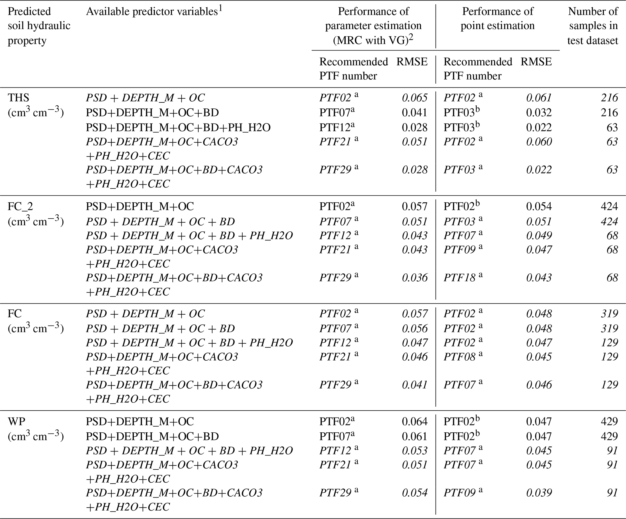
1 PSD: particle size distribution (sand, 50–2000 µm; silt, 2–50 µm; clay, < 2 µm (mass %)); DEPTH: mean soil depth (cm); OC: organic carbon content (mass %); BD: bulk density (g cm−3); CACO3: calcium carbonate content (mass %); PH_H2O: pH in water (–); CEC: cation exchange capacity (cmol (+) kg−1). 2 MRC: moisture retention curve; VG: parameters of the van Genuchten model. Different letters in a row indicate significant differences at the 0.05 level between the accuracy of the methods based on the squared error; for example performance indicated with the letter b is significantly better than the one noted with letter a. RMSE: root mean squared error.
Table 10The results of comparing the performance of euptfv1 and euptfv2 on the test sets of EU-HYDI to predict soil hydraulic properties. Rows in italic indicate cases where there was no significant difference between the two PTFs.
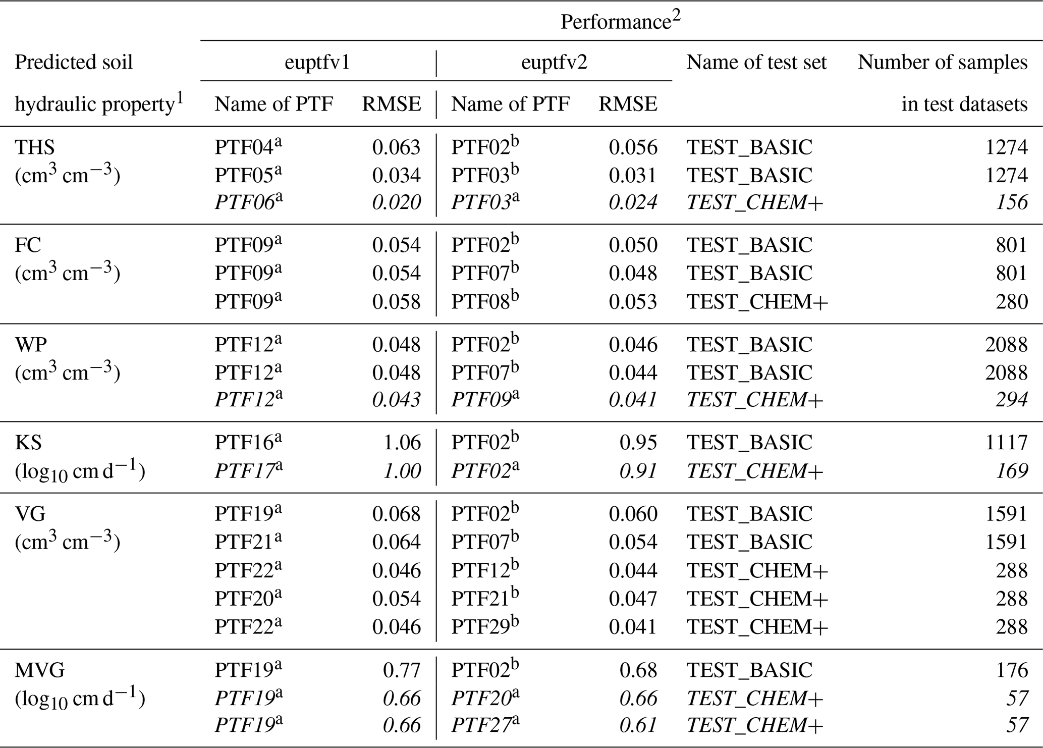
1 THS: saturated water content (pF 0); FC_2: water content at −100 cm matric potential head (pF 2.0); FC: water content at −330 cm matric potential head (pF 2.5); WP: water content at wilting point (pF 4.2); KS: saturated hydraulic conductivity; VG: parameters of the van Genuchten model; MVG: parameters of the Mualem – van Genuchten model. 2 Different letters in a row indicate significant differences at the 0.05 level between the accuracy of the methods based on the squared error;for example performance indicated with the letter b is significantly better than the one noted with letter a. RMSE: root mean squared error; TEST_BASIC: samples with measured PSD, DEPTH, OC and BD; TEST_CHEM+: samples with measured PSD, DEPTH, OC, BD, CACO3, PH_H2O and CEC; N: number of samples.
3.5 Comparison of euptfv1 and v2
The euptfv2 performs significantly better than euptfv1 in 14 out of 19 cases. In the remaining 5 cases, there is no significant difference (Table 10). Predictions of FC and MRC improve in all cases. The most important reason for it can be that the interaction between the target variable and the predictors is more complex for the cases of predicting FC or VG parameters, which can be untangled using random forest. This may provide a reason the random forest algorithm performed significantly better than the PTFs derived with linear regression or a simple regression tree. For THS, WP, KS, and MVG only those PTFs did not improve significantly, for which comparisons on the TEST_CHEM+ set were possible – which includes a reduced number of samples. The RMSE of THS prediction was somewhat lower for euptfv1 than for euptfv2, but the difference was not significant. It could be due to the close to linear relationship between THS and BD and high relative importance of BD in THS prediction (84 %). This way their interaction can be efficiently described with the linear regression which is capable to extrapolate as well. Extrapolation with the random forest algorithm is not possible outside the training data, which can limit its performance. The general improvement of the PTFs in euptfv2 is threefold, the better performance is due to (i) using random forest instead of single regression tree or linear regression, (ii) including more detailed information on soil sampling depth, not only distinguishing topsoils and subsoils and (iii) providing information on prediction uncertainty.
We recommend the use of euptfv2 instead of euptfv1 if continuous soil properties are available. If only texture classes – i.e. no particle size distribution – are available, class PTFs of euptfv1 can be used, that is PTF18 for modified FAO texture classes and PTF19 for USDA texture classes.
Table 11List of recommended pedotransfer functions (PTFs) by predicted soil hydraulic property and available predictor variables.
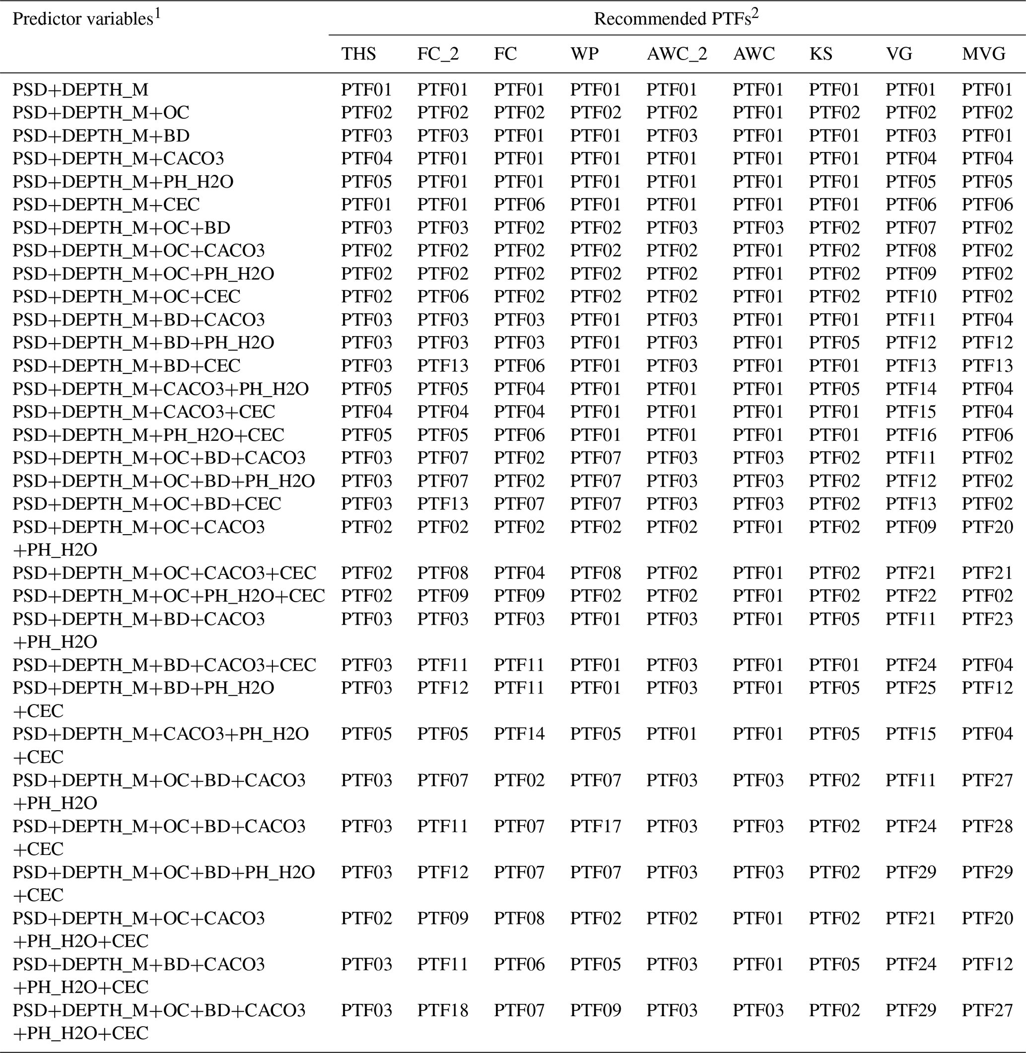
1 PSD: particle size distribution (sand, 50–2000 µm; silt, 2–50 µm; clay, < 2 µm (mass %)); DEPTH: mean soil depth (cm); OC: organic carbon content (mass %); BD: bulk density (g cm−3); CACO3: calcium carbonate content (mass %); PH_H2O: pH in water (–); CEC: cation exchange capacity (cmol (+) kg−1). 2THS: saturated water content (pF 0); FC_2: water content at -100 cm matric potential head (pF 2.0); FC: water content at -330 cm matric potential head (pF 2.5); AWC_2: plant available water content based on FC_2; AWC: plant available water content based on FC; WP: water content at wilting point (pF 4.2); KS: saturated hydraulic conductivity; VG: parameters of the van Genuchten model; MVG: parameters of the Mualem – van Genuchten model; TEST_BASIC: samples with measured PSD, DEPTH, OC and BD; TEST_CHEM+: samples with measured PSD, DEPTH, OC, BD, CACO3, PH_H2O and CEC.
The minimum input requirements for all PTFs are sand, silt and clay content, and soil depth. Soil depth is defined as the mean sampling depth, e.g. if PSD, BD and OC are provided for a soil sample from a depth of 0–20 cm, then the soil depth input (DEPTH) to the prediction algorithm is set to 10 cm.
If only soil texture information is available for the predictions, the class PTFs from euptfv1 could be applied (Tóth et al., 2015).
We emphasize that:
-
the units of input soil properties (predictors) have to be the same as indicated in the text and that the sand, silt, and clay are defined by the following particle diameters: clay <2 µm, silt between 2 and 50 µm, and sand between 50 and 2000 µm,
-
when only specific water content values at saturation, field capacity or wilting point are required (i.e. THS, FC_2, FC, WP) it is recommended to use point PTFs. This is also true for the prediction of KS,
-
for AWC, the most accurate way is to predict FC and WP with the point predictions, first, and then compute AWC using Eq. (1), and similarly for AWC_2 using FC_2 and Eq. (2),
-
it is recommended to do the VG prediction if only moisture retention curve parameters are needed, and
-
the MVG prediction when both moisture retention and hydraulic conductivity parameters are required.
The VG algorithms predict the following van Genuchten model parameters: the residual water content θr (cm3 cm−3), the saturated water content θs (cm3 cm−3), and shape parameters α (cm−1) and n (–). Parameter m (–) is provided based on (van Genuchten, 1980), and for the MVG algorithms, the two additional parameters: K0 (cm d−1) the hydraulic conductivity acting as a matching point at saturation and L (–), a shape parameter related to pore tortuosity.
Table 11 shows the recommended PTFs for each predicted soil hydraulic property and available predictor variables. The users need to check which basic soil properties are available for the predictions, then look in Table 11 which PTF is recommended to use.
The algorithms have been implemented in a web interface to facilitate the use of the PTFs, where the PTFs' selection is automated based on soil properties available for the predictions and required soil hydraulic property. The Code and data availability section provides information on how to access this resource.
The updated EU-PTFs – euptfv2 – perform significantly better than euptfv1 and are applicable for 32 predictor variables combinations. Uncertainties of the predicted soil hydraulic properties and model parameters can be computed. These uncertainties are, without further discrimination, related to the considered input data, predictors and the applied algorithm. The euptfv2 includes transfer functions to compute soil water content at saturation (0 cm matric potential head), field capacity (both −100 and −330 cm matric potential head) and wilting point (−15 000 cm matric potential head), plant available water content computed with field capacity at −100 and −330 cm matric potential head, saturated hydraulic conductivity, and Mualem–van Genuchten parameters of the moisture retention and hydraulic conductivity curves. For analyses of the impact as well as the significance of the uncertainties on the predicted soil hydraulic properties and model parameters, further studies are required.
The current version of euptfv2 is available from a user friendly web interface: https://ptfinterface.rissac.hu (last access: 4 January 2021, Szabó et al., 2019b) under the Creative Commons Attribution-NonCommercial 3.0 Unported License. The exact version of the model used to produce the results used in this paper is archived on Zenodo (https://doi.org/10.5281/ZENODO.3759442, Szabó et al., 2020), as are the R scripts to develop the predictions and the derived pedotransfer functions – in RData format – presented in this paper. The training data set cannot be made publicly available due to legal restrictions of the EU-HYDI dataset, thus only a test sample is provided along with the model code. The R files are complied into an R package to use the pedotransfer functions, archived on Zenodo (https://doi.org/10.5281/zenodo.4281045, Weber et al., 2020b).
The supplement related to this article is available online at: https://doi.org/10.5194/gmd-14-151-2021-supplement.
BS, TKDW and MW conceptualized the study and designed the methodology. BS supervised the research. MW cured the EU-HYDI dataset. BS, TKDW and MW prepared scripts for the statistical analysis, BS carried out the formal analysis, visualization and coordinated building of the PTF web interface. TKDW and BS built the R package with contributions of MW. BS and TKDW performed the validation. BS and TKDW wrote the paper with considerable input from MW.
The authors declare that they have no conflict of interest.
We are grateful to the individual scientists and their institutions in Europe who contributed to the establishment of the EU-HYDI database. We thank Gergely Tóth and Luca Montanarella for supporting the initiative that led to the EU-HYDI database. On behalf of the János Bolyai Research Scholarship we are grateful for the use of the MTA Cloud (https://cloud.mta.hu/, last access: 4 January 2021), which significantly helped us achieve the results published in this paper. We wish to thank Jeromos Rózsa for defining the computing infrastructure. We also thank Dávid Gyurkó for building the web interface for the prediction algorithms.
This research has been supported by the Hungarian National Research, Development and Innovation Office (grant no. KH124765), the János Bolyai Research Scholarship of the Hungarian Academy of Sciences (grant no. BO/00088/18/4), and the German Research Foundation (grant no. SFB 1253/1 2017).
This paper was edited by Wolfgang Kurtz and reviewed by three anonymous referees.
Araya, S. N. and Ghezzehei, T. A.: Using Machine Learning for Prediction of Saturated Hydraulic Conductivity and Its Sensitivity to Soil Structural Perturbations, Water Resour. Res., 55, 5715–5737, https://doi.org/10.1029/2018WR024357, 2019.
Assouline, S. and Or, D.: Conceptual and Parametric Representation of Soil Hydraulic Properties: A Review, Vadose Zone J., 12, 1–20, https://doi.org/10.2136/vzj2013.07.0121, 2013.
Børgesen, C. D. and Schaap, M. G.: Point and parameter pedotransfer functions for water retention predictions for Danish soils, Geoderma, 127, 154–167, https://doi.org/10.1016/j.geoderma.2004.11.025, 2005.
Botula, Y.-D., Nemes, A., Mafuka, P., Van Ranst, E., and Cornelis, W. M.: Prediction of Water Retention of Soils from the Humid Tropics by the Nonparametric -Nearest Neighbor Approach, Vadose Zone J., 12, 1–17, https://doi.org/10.2136/vzj2012.0123, 2013.
Boulesteix, A. L., Janitza, S., Kruppa, J., and König, I. R.: Overview of random forest methodology and practical guidance with emphasis on computational biology and bioinformatics, Wires. Data Min. Knowl., 2, 493–507, https://doi.org/10.1002/widm.1072, 2012.
Breiman, L.: Random Forests, Mach. Learn., 45, 5–32, 2001.
Deng, H., Ye, M., Schaap, M. G., and Khaleel, R.: Quantification of uncertainty in pedotransfer function-based parameter estimation for unsaturated flow modeling, Water Resour. Res., 45, W04409, https://doi.org/10.1029/2008WR007477, 2009.
van Genuchten, M. T.: A closed-form equation for predicting the hydraulic conductivity of unsaturated soils, Soil Sci. Soc. Am. J., 44, 892–898, 1980.
Greenwell, B.: Partial Dependence Plots, 15, available at: https://cran.r-project.org/web/packages/pdp/pdp.pdf (last access: 4 January 2021), 2017a.
Greenwell, B. M.: pdp: An R Package for Constructing Partial Dependence Plots, R J., 9, 421–436, available at: https://journal.r-project.org/archive/2017/RJ-2017-016/RJ-2017-016.pdf (last access: 4 January 2021), 2017b.
Hastie, T., Tibshirani, R., and Friedman, J.: The Elements of Statistical Learning, Data Mining, Inference, and Prediction, 2nd Edn., Springer, available at: https://web.stanford.edu/~hastie/ElemStatLearn//printings/ESLII_print10.pdf (last access: 19 November 2018), 2009.
Hengl, T., Nussbaum, M., Wright, M. N., and Heuvelink, B. M.: Random Forest as a Generic Framework for Predictive Modeling of Spatial and Spatio-temporal Variables, PeerJ Prepr., 6, e5518, https://doi.org/10.7287/peerj.preprints.26693v3, 2018.
Hodnett, M. G. and Tomasella, J.: Marked differences between van Genuchten soil water-retention parameters for temperate and tropical soils: a new water-retention pedo-transfer functions developed for tropical soils, Geoderma, 108, 155–180, https://doi.org/10.1016/S0016-7061(02)00105-2, 2002.
Khodaverdiloo, H., Homaee, M., van Genuchten, M. T., and Dashtaki, S. G.: Deriving and validating pedotransfer functions for some calcareous soils, J. Hydrol., 399, 93–99, https://doi.org/10.1016/j.jhydrol.2010.12.040, 2011.
Kotlar, A. M., Jong van Lier, Q., Barros, A. H. C., Iversen, B. V., and Vereecken, H.: Development and Uncertainty Assessment of Pedotransfer Functions for Predicting Water Contents at Specific Pressure Heads, Vadose Zo.ne J., 18, 190063, https://doi.org/10.2136/vzj2019.06.0063, 2019.
Kuhn, M., Wing, J., Weston, S., Williams, A., Keefer, C., Engelhardt, A., Cooper, T., Mayer, Z., Benesty, M., Lescarbeau, R., Ziem, A., Scrucca, L., Tang, Y., Candan, C., and Hunt, T.: Package “caret” Classification and Regression Training Description Misc functions for training and plotting classification and regression models, available at: https://cran.r-project.org/web/packages/caret/caret.pdf (last access: 4 January 2021), 2017.
Kuhn, M., Wing, J., Weston, S., Keefer, C., Engelhardt, A., Cooper, T., Mayer, Z., Kenkel, B., Team, R. C., Benesty, M., Lescarbeau, R., Ziem, A., Scrucca, L., Tang, Y., Candan, C., and Hunt, T.: caret: Classification and Regression Training. R package version 6.0-79, available at: https://github.com/topepo/caret/ (last access: 4 January 2021), 2018.
Lal, R. and Shukla, M. K.: Principles of soil physics, Marcel Dekker, Inc., New York, 2004.
Li, D., Gao, G., and Fu, B.: Predicting available water of soil from particle-size distribution and bulk density in an oasis – desert transect in northwestern China, J. Hydrol., 538, 539–550, https://doi.org/10.1016/j.jhydrol.2016.04.046, 2016.
Lilly, A., Nemes, A., Rawls, W. J., and Pachepsky, Y. A.: Probabilistic approach to the identification of input variables to estimate hydraulic conductivity, Soil Sci. Soc. Am. J., 72, 16–24, https://doi.org/10.2136/sssaj2006.0391, 2008.
Lin, H.: Earth's Critical Zone and hydropedology: concepts, characteristics, and advances, Hydrol. Earth Syst. Sci., 14, 25–45, https://doi.org/10.5194/hess-14-25-2010, 2010.
Van Looy, K., Bouma, J., Herbst, M., Koestel, J., Minasny, B., Mishra, U., Montzka, C., Nemes, A., Pachepsky, Y. A., Padarian, J., Schaap, M. G., Tóth, B., Verhoef, A., Vanderborght, J., van der Ploeg, M. J., Weihermüller, L., Zacharias, S., Zhang, Y., and Vereecken, H.: Pedotransfer Functions in Earth System Science: Challenges and Perspectives, Rev. Geophys., 55, 1199–1256, https://doi.org/10.1002/2017RG000581, 2017.
Malone, B. P., McBratney, A. B., Minasny, B., and Laslett, G. M.: Mapping continuous depth functions of soil carbon storage and available water capacity, Geoderma, 154, 138–152, https://doi.org/10.1016/j.geoderma.2009.10.007, 2009.
McNeill, S. J., Lilburne, L. R., Carrick, S., Webb, T. H., and Cuthill, T.: Pedotransfer functions for the soil water characteristics of New Zealand soils using S-map information, Geoderma, 326, 96–110, https://doi.org/10.1016/j.geoderma.2018.04.011, 2018.
Meinshausen, N.: Quantile Regression Forests, J. Mach. Learn. Res., 7, 983–999, 2006.
De Mendiburu, F.: agricolae: Statistical Procedures for Agricultural Research, R package version 1.2-8, available at: https://cran.r-project.org/package=agricolae (last access: 4 January 2021), 2017.
Mualem, Y.: A new model for predicting the hydraulic conductivity of unsaturated porous media, Water Resour. Res., 12, 513–522, 1976.
Nemes, A., Schaap, M., and Wösten, J.: Functional evaluation of pedotransfer functions derived from different scales of data collection, Soil Sci. Soc. Am., 67, 1093–1102, 2003.
Nguyen, P. M., Haghverdi, A., Pue, J. De, Botula, Y., Le, K. V, Waegeman, W., and Cornelis, W. M.: Comparison of statistical regression and data-mining techniques in estimating soil water retention of tropical delta soils, Biosyst. Eng., 153, 12–27, https://doi.org/10.1016/j.biosystemseng.2016.10.013, 2017.
Nussbaum, M., Spiess, K., Baltensweiler, A., Grob, U., Keller, A., Greiner, L., Schaepman, M. E., and Papritz, A.: Evaluation of digital soil mapping approaches with large sets of environmental covariates, SOIL, 4, 1–22, https://doi.org/10.5194/soil-4-1-2018, 2018.
Odgers, N. P., McBratney, A. B., and Minasny, B.: Digital soil property mapping and uncertainty estimation using soil class probability rasters, Geoderma, 237, 190–198, https://doi.org/10.1016/j.geoderma.2014.09.009, 2014.
Olson, R. S., La Cava, W., Mustahsan, Z., Varik, A., and Moore, J. H.: Data-driven advice for applying machine learning to bioinformatics problems, in Biocomputing 2018, edited by: Altman, R. B., Dunker, A. K., Hunter, L., Ritchie, M. D., Murray, T. A., and Klein, T. E., World Scientific, 192–203, 2018.
Pachepsky, Y. A. and Rawls, W. J.: Accuracy and Reliability of Pedotransfer Functions as Affected by Grouping Soils, Soil Sci. Soc. Am. J., 63, 1748–1757, https://doi.org/10.2136/sssaj1999.6361748x, 1999.
R Core Team: R: A language and environment for statistical computing, available at: https://www.r-project.org (last access: 4 January 2021), 2019.
Rawls, W., Pachepsky, Y., and Ritchie, J.: Effect of soil organic carbon on soil water retention, Geoderma, 116, 61–76, https://doi.org/10.1016/S0016-7061(03)00094-6, 2003.
Ridgeway, G.: gbm: Generalized Boosted Regression Models, R package version 2.1.3., 2017.
Román Dobarco, M., Cousin, I., Le Bas, C., and Martin, M. P.: Pedotransfer functions for predicting available water capacity in French soils, their applicability domain and associated uncertainty, Geoderma, 336, 81–95, https://doi.org/10.1016/J.GEODERMA.2018.08.022, 2019.
Schaap, M. G.: Models for Indirect Estimation of Soil Hydraulic Properties, in Encyclopedia of Hydrological Sciences, edited by: Anderson, M. G. and McDonnell, J. J., John Wiley & Sons, Ltd, Chichester, UK, 2006.
Streck, T. and Weber, T. K. D.: Analytical expressions for noncapillary soil water retention based on popular capillary retention models, Vadose Zone J., 19, e20042, https://doi.org/10.1002/vzj2.20042, 2020.
Szabó, B., Szatmári, G., Takács, K., Laborczi, A., Makó, A., Rajkai, K., and Pásztor, L.: Mapping soil hydraulic properties using random-forest-based pedotransfer functions and geostatistics, Hydrol. Earth Syst. Sci., 23, 2615–2635, https://doi.org/10.5194/hess-23-2615-2019, 2019a.
Szabó, B., Gyurkó, D., Weynants, M., and Weber, T. K. D.: Web interface for European hydraulic pedotransfer functions (euptfv2), Agártudományi Kutatóközpont, Talajtani Intézet, https://doi.org/10.34977/euptfv2.01, 2019b.
Szabó, B., Weynants, M., and Weber, T. K.: Scripts of updated European hydraulic pedotransfer functions (euptfv2), Zenodo, https://doi.org/10.5281/ZENODO.3759442, 2020.
Szatmári, G. and Pásztor, L.: Comparison of various uncertainty modelling approaches based on geostatistics and machine learning algorithms, Geoderma, 337, 1329–1340, https://doi.org/10.1016/j.geoderma.2018.09.008, 2019.
Tomasella, J., Crestana, S. and Rawls, W. J.: Comparison of Two Techniques to Develop Pedotransfer Functions for Water Retention, Soil Sci. Soc. Am. J., 67, 1085–1092, 2003.
Tóth, B., Weynants, M., Nemes, A., Makó, A., Bilas, G., and Tóth, G.: New generation of hydraulic pedotransfer functions for Europe, Eur. J. Soil Sci., 66, 226–238, https://doi.org/10.1111/ejss.12192, 2015.
Tóth, B., Weynants, M., Pásztor, L., and Hengl, T.: 3D soil hydraulic database of Europe at 250 m resolution, Hydrol. Process., 31, 2662–2666, https://doi.org/10.1002/hyp.11203, 2017.
Tranter, G., Minasny, B., and McBratney, A. B.: Estimating Pedotransfer Function Prediction Limits Using Fuzzy -Means with Extragrades, Soil Sci. Soc. Am. J., 74, 1967–1975, https://doi.org/10.2136/sssaj2009.0106, 2010.
Vaysse, K. and Lagacherie, P.: Using quantile regression forest to estimate uncertainty of digital soil mapping products, Geoderma, 291, 55–64, https://doi.org/10.1016/j.geoderma.2016.12.017, 2017.
Vereecken, H., Maes, J., Feyen, J., and Darius, P.: Estimating the Soil Moisture Retention Characteristic From Texture, Bulk Density, and Carbon Content, Soil Sci., 148, 389–403, https://doi.org/10.1097/00010694-198912000-00001, 1989.
Vereecken, H., Huisman, J. A., Franssen Hendricks, H. J., Brüggemann, N., Bogena, H. R., Kollet, S., Javaux, M., van der Kruk, J., and Vanderborght, J.: Soil hydrology: Recent methodological advances, challenges, and perspectives, Water Resour. Res., 51, 1–18, https://doi.org/10.1002/2014WR016852.Received, 2015.
Weber, T. K. D., Durner, W., Streck, T., and Diamantopoulos, E.: A Modular Framework for Modeling Unsaturated Soil Hydraulic Properties Over the Full Moisture Range, Water Resour. Res., 55, 4994–5011, https://doi.org/10.1029/2018WR024584, 2019.
Weber, T. K. D., Finkel, M., Conceição Gonçalves, M., Vereecken, H., and Diamantopoulos, E.: Pedotransfer function for the Brunswick soil hydraulic property model and comparison to the van Genuchten-Mualem model, Water Resour. Res., 56, e2019WR026820, https://doi.org/10.1029/2019WR026820, 2020a.
Weber, T. K. D., Weynants, M., and Szabó, B.: R package of updated European hydraulic pedotransfer functions (euptf2), Zenodo, https://doi.org/10.5281/zenodo.4281045, 2020b.
Weynants, M. and Tóth, B.: The euptf package, Eur. Soil Portal, 5, available at: https://esdac.jrc.ec.europa.eu (last access: 19 May 2019), 2014.
Weynants, M., Vereecken, H., and Javaux, M.: Revisiting Vereecken Pedotransfer Functions: Introducing a Closed-Form Hydraulic Model, Vadose Zone J., 8, 86, https://doi.org/10.2136/vzj2008.0062, 2009.
Weynants, M., Montanarella, L., Tóth, G., Arnoldussen, A., Anaya Romero, M., Bilas, G., Borresen, T., Cornelis, W., Daroussin, J., Gonçalves, M. D. C., Haugen, L.-E., Hennings, V., Houskova, B., Iovino, M., Javaux, M., Keay, C. A., Kätterer, T., Kvaerno, S., Laktinova, T., Lamorski, K., Lilly, A., Mako, A., Matula, S., Morari, F., Nemes, A., Patyka, N. V., Romano, N., Schindler, U., Shein, E., Slawinski, C., Strauss, P., Tóth, B., and Woesten, H.: European HYdropedological Data Inventory (EU-HYDI), Scientific and Technical Research series, ISSN 1831-9424, Luxembourg, 2013.
Wiesmeier, M., Urbanski, L., Hobley, E., Lang, B., von Lützow, M., Marin-Spiotta, E., van Wesemael, B., Rabot, E., Ließ, M., Garcia-Franco, N., Wollschläger, U., Vogel, H. J. and Kögel-Knabner, I.: Soil organic carbon storage as a key function of soils - A review of drivers and indicators at various scales, Geoderma, 333, 149–162, https://doi.org/10.1016/j.geoderma.2018.07.026, 2019.
Wösten, J. H. M., Lilly, A., Nemes, A., and Le Bas, C.: Development and use of a database of hydraulic properties of European soils, Geoderma, 90, 169–185, 1999.
Wright, M. N. and Ziegler, A.: ranger: A Fast Implementation of Random Forests for High Dimensional Data in C and R, J. Stat. Softw., 77, 1–17, https://doi.org/10.18637/jss.v077.i01, 2017.
Zhang, Y. and Schaap, M. G.: Weighted recalibration of the Rosetta pedotransfer model with improved estimates of hydraulic parameter distributions and summary statistics (Rosetta3), J. Hydrol., 547, 39–53, https://doi.org/10.1016/j.jhydrol.2017.01.004, 2017.
Zhang, Y. and Schaap, M. G.: Estimation of saturated hydraulic conductivity with pedotransfer functions: A review, J. Hydrol., 575, 1011–1030, https://doi.org/10.1016/j.jhydrol.2019.05.058, 2019.
Zhao, H., Zeng, Y., Lv, S., and Su, Z.: Analysis of soil hydraulic and thermal properties for land surface modeling over the Tibetan Plateau, Earth Syst. Sci. Data, 10, 1031–1061, https://doi.org/10.5194/essd-10-1031-2018, 2018.
Ziegler, A. and König, I. R.: Mining data with random forests: Current options for real-world applications, Wires Data Min. Knowl., 4, 55–63, https://doi.org/10.1002/widm.1114, 2014.