The Regional Ice Ocean Prediction System v2: a pan-Canadian ocean analysis system using an online tidal harmonic analysis

Canada has the longest coastline in the world and includes diverse ocean environments, from the frozen waters of the Canadian Arctic Archipelago to the confluence region of Labrador and Gulf Stream waters on the east coast. There is a strong need for a pan-Canadian operational regional ocean prediction capacity covering all Canadian coastal areas in support of marine activities including emergency response, search and rescue, and safe navigation in ice-infested waters. Here we present the first pan-Canadian operational regional ocean analysis system developed as part of the Regional Ice Ocean Prediction System version 2 (RIOPSv2) running in operations at the Canadian Centre for Meteorological and Environmental Prediction (CCMEP). The RIOPSv2 domain extends from 26^∘ N in the Atlantic Ocean through the Arctic Ocean to 44^∘ N in the Pacific Ocean, with a model grid resolution that varies between 3 and 8 km. RIOPSv2 includes a multivariate data assimilation system based on a reduced-order extended Kalman filter together with a 3D-Var bias correction system for water mass properties. The analysis system assimilates satellite observations of sea level anomaly and sea surface temperature, as well as in situ temperature and salinity measurements. Background model error is specified in terms of seasonally varying model anomalies from a 10-year forced model integration, allowing inhomogeneous anisotropic multivariate error covariances. A novel online tidal harmonic analysis method is introduced that uses a sliding-window approach to reduce numerical costs and allow for the time-varying harmonic constants necessary in seasonally ice-infested waters. Compared to the Global Ice Ocean Prediction System (GIOPS) running at CCMEP, RIOPSv2 also includes a spatial filtering of model fields as part of the observation operator for sea surface temperature (SST). In addition to the tidal harmonic analysis, the observation operator for sea level anomaly (SLA) is also modified to remove the inverse barometer effect due to the application of atmospheric pressure forcing fields. RIOPSv2 is compared to GIOPS and shown to provide similar innovation statistics over a 3-year evaluation period. Specific improvements are found near the Gulf Stream for all model fields due to the higher model grid resolution, with smaller root mean squared (rms) innovations for RIOPSv2 of about 5 cm for SLA and 0.5 ^∘C for SST. Verification against along-track satellite observations demonstrates the improved representation of mesoscale features in RIOPSv2 compared to GIOPS, with increased correlations of SLA (0.83 compared to 0.73) and reduced rms differences (12 cm compared to 14 cm). While the RIOPSv2 grid resolution is 3 times higher than GIOPS, the power spectral density of surface kinetic energy provides an indication that the effective resolution of RIOPSv2 is roughly double that of the global system (35 km compared to 66 km). Observations made as part of the Year of Polar Prediction (2017–2019) provide a rare glimpse at errors in Arctic water mass properties and show average salinity biases over the upper 500 m of 0.3–0.4 psu in the eastern Beaufort Sea in RIOPSv2.

1 Introduction

Over recent years, there has been a growing number of regional ocean prediction systems developed and being run operationally (Kourafalou et al., 2015; Tonani et al., 2015). For example, as part of the European Copernicus Marine Environmental Monitoring Service (CMEMS) there are regional systems covering the Arctic Ocean (Sakov et al., 2012), the northwest European shelf seas (King et al., 2018), the Iberia–Biscay–Ireland (IBI) shelf seas (Sotillo et al., 2015), the Mediterranean Sea (Tonani et al., 2008), and the Baltic Sea (Zhuang et al., 2011). Various systems are also in place along the US coastlines (e.g., Zhang et al., 2010; Moore et al., 2011; Xue et al., 2005; Mehra and Rivin, 2010; Chao et al., 2018). More recently, a number of systems have been put in place by China (Cho et al., 2014), Japan (Hirose et al., 2019) and Korea (Park et al., 2015).

A particular challenge for regional ocean prediction systems is the assimilation of sea level anomaly (SLA) observations into an ocean model that includes tidal forcing. Removing tidal variability requires a careful approach as any unfiltered tidal variations will contribute directly to the innovations and may result in unphysical increments. The approach taken in the IBI system is to perform an offline harmonic analysis and apply a static set of harmonic coefficients for the primary tidal constituents to remove tidal signals during the online assimilation step. However, this approach neglects nonstationary effects such as seasonally varying interactions between barotropic and baroclinic tidal modes. Moreover, in areas of sea ice cover, a strong seasonal cycle in tidal harmonics may be present. Indeed, Kleptsova and Pietrzak (2018) show summer–winter differences in the M2 amplitude that exceed 1 m in Hudson Strait and Ungava Bay, with changes in phase up to 180^∘ due to the displacement of tidal amphidromes. Xie et al. (2011) find that a 3 d mean filter provides a suitable reduction in tidal variance in the South China Sea to permit SLA assimilation but note that more sophisticated filters may provide better results.

Developing a regional ocean prediction system for Canada is challenging due to the length of the Canadian coastline and complexity of coastal waters in Canada. First, Canada's coasts cover three oceans that differ greatly, from relatively warm North Pacific Ocean waters on the west coast, to the confluence region of the Gulf Stream and the Labrador Current on the east coast, and to seasonal and multiyear sea ice in the Canadian Arctic Archipelago. Moreover, all three regions experience strong tidal currents, including the two largest tidal ranges in the world in the Bay of Fundy and Ungava Bay (Arbic et al., 2007; O'Reilly et al., 2005). A paucity of in situ data further complicates the development of reliable data assimilative operational oceanographic systems due in particular to significant gaps in real-time data availability. This situation is especially challenging in the Canadian Arctic Archipelago due to the harsh environmental conditions, combined with dynamic sea ice cover, and is further complicated by significant regions of poorly known bathymetry.

Early efforts in operational oceanography in Canada include models run in real time without any data assimilation to support search and rescue as well as oil spill response for the Gulf of St. Lawrence (Saucier et al., 2003) and St. Lawrence Estuary (Saucier and Chassé, 2000). The Gulf of St. Lawrence model was later developed into a coupled prediction system for sea ice and weather prediction (Pellerin et al., 2004; Smith et al., 2012). Additionally, a coupled ice–ocean prediction system for the Canadian east coast used for iceberg drift, ice service operations (i.e., for safe navigation), and offshore resource exploitation was implemented in 2007 that assimilates sea surface temperature and ice concentration (Tang et al., 2008). On the Canadian west coast there have been numerous modeling efforts (e.g., Masson and Cummins, 2007) but few real-time forecasting efforts, apart from tidal and storm surge forecasting systems (e.g., Soontiens et al., 2016).

More recently, the Global Ice Ocean Prediction System (GIOPS) was implemented at the Canadian Centre for Meteorological and Environmental Prediction (CCMEP), providing the first operational global ocean assimilative capacity in Canada (Smith et al., 2016). This system was designed primarily to support the initialization of coupled medium-range deterministic weather prediction (Smith et al., 2018). It is also now used to initialize coupled ensemble predictions of sub-seasonal (medium-monthly) range in addition to seasonal predictions (Lin et al., 2020). GIOPS analyses and forecasts are also used by the Canadian navy for marine operations (e.g., sonar range prediction). Building on the availability of ocean analyses from GIOPS, a higher-grid-resolution Regional Ice Ocean Prediction System (RIOPS) was developed (Dupont et al., 2015; Lemieux et al., 2016a) to support marine operations in Canadian ice-infested waters, in particular over two Arctic METAREAs (17 and 18) for which Canada has the responsibility to provide warnings regarding ice hazards and marine weather predictions as part of the Global Marine Distress and Safety System.

Increasing requirements for a world-class safety system to protect Canadian coastal areas have motivated the creation of the Government of Canada Ocean Protection Plan initiative. This initiative aims to put in place a range of measures, including pan-Canadian ocean prediction capacity to provide numerical guidance for marine emergency response (e.g., oil spill). To meet this need, ocean predictions are required that are able to represent coastal ocean processes (e.g., tidal flows, boundary currents) while constraining internal variability (i.e., through data assimilation).

There has yet to be a pan-Canadian regional ocean prediction system capable of meeting this need. Here we present the first such system in RIOPSv2, implemented operationally at the CCMEP on 3 July 2019 and developed as part of the Canadian Operational Network for Coupled Environmental Prediction Systems (CONCEPTS) initiative (Smith et al., 2013). RIOPSv2 includes both an extended domain to cover the North Pacific Ocean (Fig. 1) and a multivariate ocean data assimilation system. The ocean data assimilation component is similar to that used in the GIOPS system with several important additions. First, the sea level anomaly observation operator must be modified to filter tidal variations. Given the seasonal variations in tidal harmonics due to the presence of sea ice, a novel online harmonic analysis with a sliding-window approach is introduced. Second, a spatial filter is added to the sea surface temperature (SST) observation operator to remove small-scale features not resolved in the SST analysis product assimilated. The background error is defined in terms of a set of error modes derived from a multiyear forced simulation following the approach described by Lellouche et al. (2013). The incremental analysis updating (IAU) period is extended from 1 d used by GIOPS to 7 d to provide improved continuity. As a result, the RIOPSv2 system has many aspects in common with the CMEMS global prediction system (Lellouche et al., 2013). Particular differences include the use of a regional domain, the inclusion of tidal sea surface height (SSH) variations, a 3D-Var sea ice analysis, the assimilation of the CCMEP SST, and the use of a daily update analysis using a 1 d assimilation window to initialize forecasts.

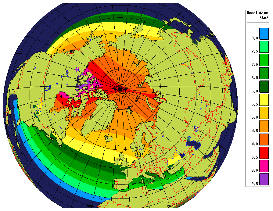
Figure 1 The coverage of the CREG12 extended domain used in RIOPSv2 showing the model grid resolution (km). The domain extends from 26^∘ N in the Atlantic Ocean over the Arctic Ocean to 44^∘ N in the Pacific Ocean. The model bathymetry is set to zero for the partially covered regions of the Gulf of Mexico, the Black and Red seas, and for inland lakes.

Here we present the RIOPSv2 system and provide an evaluation and demonstration of the added value with respect to the GIOPS analysis system. Section 2 provides a detailed description of the ocean and sea ice numerical models and describes improvements with respect to the previous RIOPSv1.3 system. Section 3 presents an overview of the assimilation components and details the various modifications made for RIOPSv2 including the new online harmonic analysis method introduced here. Section 4 presents an evaluation of innovations of sea level anomaly, SST, and temperature and salinity profiles over a 3-year reanalysis period. A comparison of RIOPSv2 and GIOPS along a particular Jason satellite altimeter track that crosses the Gulf Stream is also provided in Sect. 4, as is an analysis of the power spectral density of the surface kinetic energy fields of RIOPSv2 and GIOPS. Conclusions and a discussion of future work are provided in Sect. 5.

The main contributions of this paper are a description of the first pan-Canadian regional ocean analysis system, the development of a novel online harmonic analysis method with a sliding-window approach, and a demonstration of the added value of the RIOPSv2 analysis system compared to GIOPS in terms of smaller innovations over the Gulf Stream and higher effective resolution.

2 Numerical model description

2.1 Ocean model component

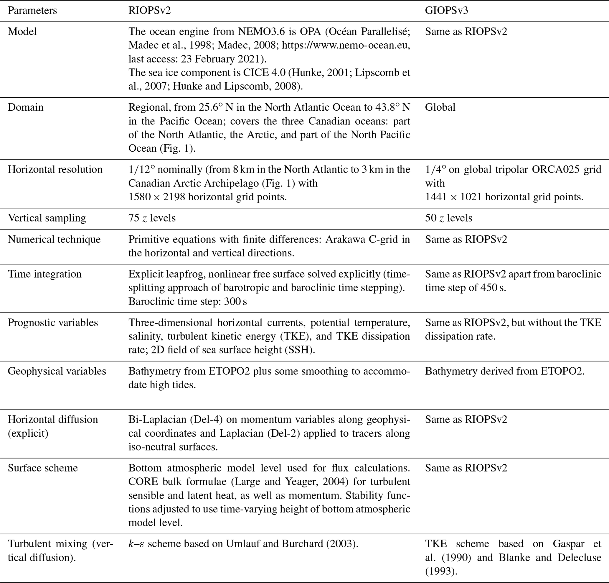
The ocean model used in RIOPSv2 and GIOPS is the Océan Parallisé (OPA) model as part of the Nucleus for European Modelling of the Ocean (NEMO; Madec et al., 2008) modeling framework. OPA is a primitive-equation model on an Arakawa C-grid employing the non-Boussinesq and hydrostatic approximations. A detailed description and evaluation of the model are provided in Dupont et al. (2015). The particular parameterization details and settings used are described in Tables 1 and 2.

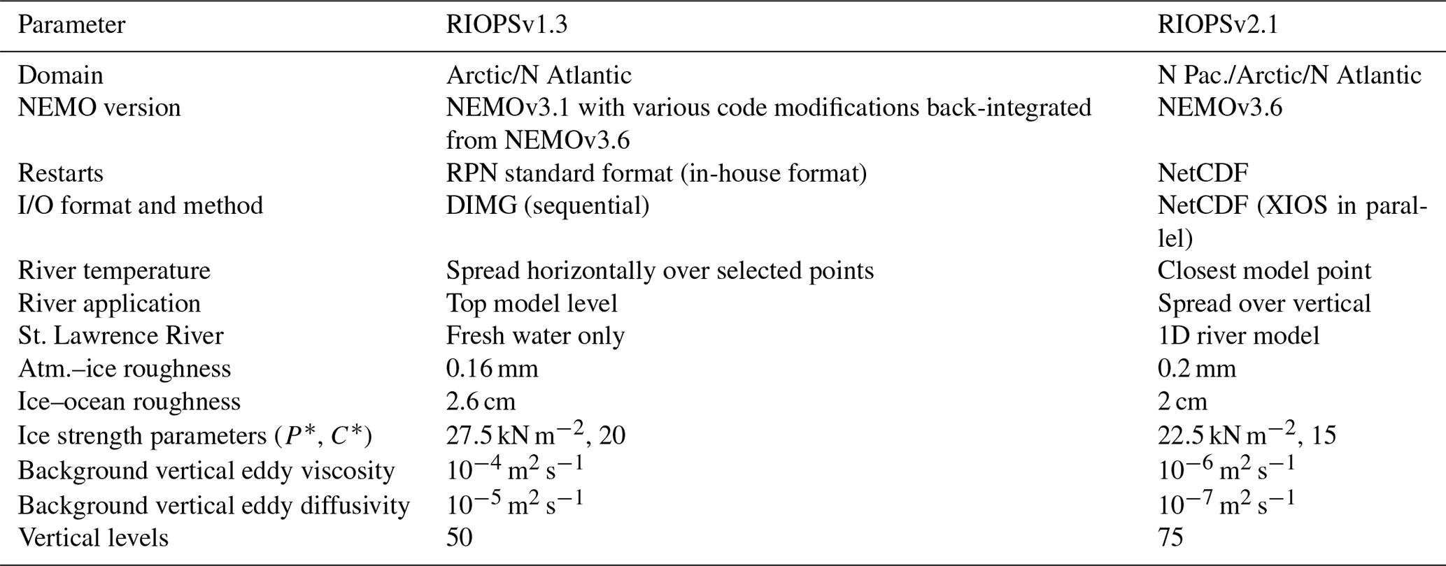
Table 1 Changes to model parameters between RIOPSv1.3 and RIOPSv2.1.

Table 2 Model parameters used in RIOPSv2 and GIOPSv3.

The RIOPSv2 numerical grid is constructed from the $\mathrm{1}/\mathrm{12}$^∘ tripolar ORCA grid (Madec and Imbard, 1996), whereby grid points from the Pacific section have been re-mapped to the top of the grid to eliminate the north fold from the ORCA grid (see Dupont et al., 2015, for details). The resulting grid has been previously referred to as the CONCEPTS regional grid (CREG) as used in various studies (e.g., Roy et al., 2015; Chikhar et al., 2019; Boutin et al., 2020). In RIOPSv2 CREG is extended to include the North Pacific Ocean down to 44^∘ N in order to cover the Canadian west coast. Bathymetry is based on ETOPO2 (Amante and Eakins, 2009).

Open boundary conditions are specified using daily mean fields from GIOPS. Tidal variations in sea surface height (SSH) and barotropic transport are applied along the open boundaries in the Atlantic and Pacific Ocean using 13 tidal constituents (M2, S2, N2, K2, O1, K1, Q1, P1, M4, Mf, Mm, Mn4, Ms4) extracted from the Oregon State University product (Egbert and Erofeeva, 2002). Self-attraction and loading terms are prescribed following the finite-element solution (FES) 2012 tidal product (Carrère et al., 2012). An evaluation of tidal variations in the CREG configuration is presented in Lemieux et al. (2018), and regional evaluations for the $\mathrm{1}/\mathrm{12}$^∘ resolution model configuration used in RIOPSv2 can be found in Nudds et al. (2020).

In RIOPSv2, the ocean model component was updated to NEMOv3.6 (from v3.1 with various modifications). As many features from NEMOv3.6 had been back-integrated in the NEMO code version used in RIOPSv1.3, this change in code did not in itself provide any significant change to model results. Rather, the code was updated to permit use of the XIOS I/O server.

Several other changes were made to the ocean model configuration (Table 1). The number of vertical levels was increased from 50 to 75 levels in order to improve the resolution of the layers from 250 to 500 m. Atmospheric pressure forcing is added such that the atmospheric pressure gradient may be applied in the momentum equations (the so-called “inverse barometer” effect) as in storm surge modeling. Following stability tests, the time step was increased to 300 s. A two-equation k–ε turbulent mixing scheme is introduced (Umlauf and Burchard, 2003) to replace the single prognostic equation turbulent kinetic energy (TKE) scheme used previously (Blanke and Delacluse, 1993). The vertical background diffusivity and viscosity were respectively reduced to molecular values (10⁻⁷ and 10⁻⁶ m² s⁻¹) to reduce mixing in deeper water masses in the Arctic.

2.2 Sea ice model component

RIOPSv2 uses the Los Alamos Community Ice CodE version 4.0 (CICE; Hunke, 2001; Lipscomb et al., 2007; Hunke and Lipscomb, 2008). CICE is a dynamic–thermodynamic sea ice model on an Arakawa B-grid. Ice–ice interactions are governed using an elasto-viscous–plastic scheme (Hunke et al., 2001). In RIOPS, CICE is configured to use 10 ice thickness categories and a single snow layer. Landfast ice is parameterized using the basal-stress approach of Lemieux et al. (2015, 2016b).

In RIOPSv2 the model code and settings were kept identical with the exception of the atmosphere–ice and ice–ocean drag coefficients and the ice strength parameters (Table 1). In an attempt to reduce the existing negative bias in ice velocity, the ice–ocean roughness was reduced from 2.6 to 2.0 cm, and the air–ice roughness was increased from 0.16 to 0.20 mm. Additionally, following Ungermann et al. (2017) and Chikhar et al. (2019), the ice strength parameters P^* and C^* were reduced to 22.5 and 15 kN m⁻², respectively (Table 1). In multi-annual hindcast simulations produced over the period 2003–2008 these changes were found to reduce the negative bias in ice drift with respect to buoys from the International Arctic Buoy Program (Rigor and Ortmeyer, 2004) as well as the gridded drift product from the National Snow and Ice Data Centre (Tschudi et al., 2019; not shown).

3 Data assimilation methods

In this section, we present the data assimilation systems for the ocean and sea ice. The main innovation introduced here is the online harmonic analysis method with a sliding-window approach described in Sect. 3.4. The gridded sea ice concentration and sea surface temperature analyses assimilated by RIOPSv2 are independent of (i.e., not cycled with) the ocean data assimilation system, and only a brief description is provided. Note that the version of RIOPS running operationally at CCMEP is expected to be updated in fall 2021 to the version of RIOPS described here (v2.1) (referred to hereafter simply as RIOPSv2).

In place of the spectral nudging approach used to generate initial conditions for RIOPSv1, in RIOPSv2 a multivariate data assimilation approach is implemented. This system is based on the System d'Assimilation Mercator version 2 (SAM2; Lellouche et al., 2013) used for GIOPS (Smith et al., 2016, 2019a). This system assimilates satellite observations of sea level anomaly and sea surface temperature, together with in situ observations of temperature and salinity. Ongoing evaluations (e.g., Zedel et al., 2018) and intercomparison activities as part of GODAE Oceanview (Bell et al., 2015) have shown GIOPS to provide analyses and forecasts of similar skill as other operational global ocean forecasting systems (Ryan et al., 2015; Divakaran et al., 2015). Following the approach used in GIOPS, the RIOPS system has three assimilation cycles (Fig. 2): a daily update (assimilating only SST and sea ice concentration with a 1 d analysis window) called “RU” (RIOPS update cycle), a real-time weekly cycle “RR” (RIOPS real-time cycle), and a delayed weekly cycle “RD” (RIOPS delayed-mode cycle) run 7 d behind real time. The RD cycle is the backbone of the system and provides the continuity in time. Both RR and RD cycles assimilate all available observations, although RD uses a longer cutoff and thus includes a greater number of in situ and SLA observations. The evaluation presented here uses RD cycles. This three-level approach is similar to the “one-way” coupled assimilation approach described in Browne et al. (2019).

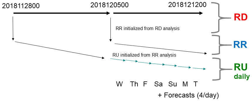
Figure 2 Schematic diagram showing the sequencing of the delayed-mode (RD), real-time (RR), and daily update cycles (RU). The RD cycle is run 7 d behind real time each Wednesday and provides continuity in time. The RR cycle is initialized from the RD cycle and provides a real-time analysis each Wednesday. Finally, the RU cycles provide daily updates using a shorter 1 d analysis cycle assimilating only sea ice and sea surface temperature. Additionally, 48 h forecasts are produced from RU analyses four times per day (00:00, 06:00, 12:00, 18:00 Z).

As the GIOPSv3 system will be used as a reference for the evaluation presented in Sect. 4, differences between RIOPSv2 and GIOPSv3 are highlighted in the following subsections.

3.1 Overview of the ocean data assimilation system

The SAM2 ocean data assimilation system is a reduced-order extended Kalman filter using a singular evolutive extended Kalman (SEEK) filter methodology (Pham et al., 1998) with a fixed basis. The main properties and features of the scheme are as described in Lellouche et al. (2013, 2018). A brief description is provided below. In the following section, specific adaptations made in the GIOPS system (Smith et al., 2016) and used for RIOPSv2 are described.

The background error is defined in terms of a static set of multivariate error modes obtained from sub-monthly anomalies of a multiyear forced simulation. A description of the method used for the construction of these error modes is provided in Sect. 3.3.2. An adaptivity scheme based on Talagrand (1998) is applied to adjust model background error variances. Innovations are calculated during the model integration in a first guess at appropriate time (FGAT) approach. Two online quality-control checks are applied to in situ temperature and salinity profiles based on temperature and salinity innovations and dynamic height innovations. Analysis increments are applied gradually in an incremental analysis updating (IAU) approach (Bloom et al., 1996). A 3D-Var bias correction approach is used for temperature and salinity profiles using mean innovations from the previous four cycles.

In order to assess satellite observations of sea level anomaly in the observation operator, mean dynamic topography (MDT) must be first removed from the model sea surface height. As a result, errors (or inconsistencies with the model) in the mean dynamic height field used may result in systematic errors in analysis increments and persistent mean increments in some regions. Here, the hybrid product described by Lellouche et al. (2018) is used. This product combines the CNES-CLS13 MDT (Rio et al., 2014) with mean increments calculated from the Mercator Ocean GLORYS2V3 reanalysis.

Several features described in Lellouche et al. (2018; system referred to therein as PSY4V3R1) are not used here. These include a Desroziers et al. (2005) scheme to adjust observation error variances and the application of a weak constraint toward climatology in the deep ocean. An additional difference is that the sea ice assimilation is not done using SAM2 but rather with a separate 3D-Var approach (described in Sect. 3.2 below).

3.2 Adaptations of SAM2 for GIOPS

A number of modifications were made to SAM2 for use in the GIOPS system and are described in Smith et al. (2016). First, the CCMEP gridded SST analysis (Brasnett and Colan, 2016) is assimilated (as opposed to the OSTIA or AVHRR products used in Lellouche et al., 2018). This foundation SST analysis is produced on a 0.1^∘ resolution latitude–longitude grid using an optimal interpolation (OI) approach that assimilates AMSR-2, AVHRR, VIIRS, and in situ observations from moorings, ships, and drifters. The OI uses the previous day's analysis as first guess for the present day's analysis. The SST OI analysis is set to the model freezing temperature in locations where the ice concentration is greater than 0.6. Additionally, SST observations within one grid cell of the coastline are rejected. The SST OI analysis is then assimilated into SAM2 using a relatively small 0.3 ^∘C observation error. This provides a tight constraint on the SST analysis necessary to reduce initialization shock for coupled forecasts (Smith et al., 2018). Another modification required for coupled forecasts was to use 24 h averaged shortwave and longwave radiation fields to force NEMO–CICE during the analysis cycles such that there is very little diurnal warming present in the ocean analysis. Damping diurnal SST variations in the analysis fields was also found to limit initialization shock in coupled forecasts as the atmospheric analysis was produced using the foundation SST product (Smith et al., 2018).

At the end of each analysis cycle, the ocean analysis is blended with a 3D-Var sea ice concentration analysis (Buehner et al., 2013, 2016). This blending adjusts the concentration of the 10 ice thickness categories using the rescaled forecast tendency (RFT) method of Smith et al. (2016). The 3D-Var ice analyses are produced on a 10 km grid and assimilate passive microwave retrievals from SSMI and SSMI/S using the NASA Team 2 algorithm, AMSR2, ASCAT, and manual RADARSAT image analyses and ice charts from the Canadian Ice Service.

3.3 Modifications of SAM2 introduced for RIOPSv2

The SAM2 system used in GIOPS had to be adapted for use in a regional context. As a result, there are several important differences in the assimilation approach used in RIOPSv2 described in the following sections. The most notable change is the introduction of the online harmonic analysis that will be described separately in the following section (Sect. 3.4).

3.3.1 7 d incremental analysis updating

In the GIOPS system, analysis increments are applied using an incremental analysis updating (IAU; Bloom et al., 1996) approach with increments applied evenly over a 1 d period. For the delayed-mode (GD) and real-time (GR) weekly cycles this is done over the last day of the 7 d assimilation window, and for the daily cycle (GU) this is done over the full 1 d window. To provide greater consistency in time, in RIOPSv2 a 7 d IAU is used for both RD and RR cycles inspired by the methodology of Benkiran and Greiner (2008). A linearly increasing ramp is used over the first day, followed by a constant increment for days 2–7. A decreasing ramp is applied for the first day of the following cycle. This approach is also applied in systems used by Mercator Océan International (Lellouche et al., 2013, 2018).

3.3.2 Background error

As mentioned above, the background error for RIOPSv2 is specified in terms of a series of error modes derived from a multiyear forced simulation over the period 2002–2011. Sub-monthly anomalies are constructed by removing low-frequency variations using a 30 d Hanning filter. The basic methodology used to calculate the error modes is the same as used for GIOPS apart from the smoothing used in the error modes. For RIOPSv2, 49 passes of a Shapiro filter are applied to temperature and salinity fields, resulting in a roughly 1^∘ smoothing. Also, tides are removed from the SSH field using the online harmonic analysis described below prior to calculation of the sea surface height anomaly.

The resulting error modes provide a seasonally varying estimate of the background error. For a particular analysis cycle, error modes within a 90 d window around the Julian day of the analysis cycle from all 10 years of the forced simulation are used. As error modes are produced every 3 d, this provides roughly 300 error modes available for each analysis cycle.

While this approach does not provide an estimate of “errors of the day” as in an ensemble Kalman filter, it does nonetheless provide an estimate of the covariances in space and between model variables (i.e., SSH and three-dimensional fields of temperature, salinity, and zonal and meridional velocities). An example of the multivariate correlations is shown in Fig. 3. Correlations can vary considerably at different locations and between variables based on the underlying oceanographic conditions. For example, in the Gulf Stream (Fig. 3) strong correlations are present between SSH and temperature at short distances, representative of dynamic height variability in this region of strong mesoscale activity.

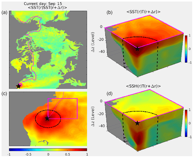
Figure 3 Example of spatial structures of multivariate correlations from background error modes for 15 September in the Gulf Stream region. The left panels show the spatial correlation of SST with the point marked with a star over the full domain (a) and over a magnified region (c). The right panels show the spatial correlation of SST with 3D temperature (b) and the spatial correlation of SSH with 3D temperature (d). The 3D cube is plotted such that the bottom left corner corresponds to the point marked with the star. The vertical dimension is plotted using the model level to enhance the resolution near the surface. Levels 20 and 40 roughly correspond to 60 and 200 m of depth, respectively. The spatial extent of the cube is shown in the left panel as a magenta box. The bubble radius used in the Gaussian localization function to reduce long-range spurious covariances is shown as a dashed oval. Model bathymetry is shown in grey. An animated version of this figure is available for which the central point marked with a star moves along the magenta line (see the Supplement).

As a SEEK filter formulation is used, the model background error will determine the subspace within which the analysis is restricted. Here, this subspace is limited by the variability of the model fields over the 10-year period of the model simulation. As such, the spatial scales represented in the analysis are determined by the effective model resolution and the spatial filtering applied to the error modes.

3.3.3 SSH observation operator

Satellite altimetry observations contain a variety of signals including those produced by tides. Here, we have chosen to address the calibration of the modeled tides separately in advance and to use the altimetry observations to constrain geostrophic variability. This permits the use of standard AVISO Ssalto/Duacs altimetry products available for operational real-time applications as required by RIOPS. These products undergo a number of processing steps to remove tidal signals, as well as wet-tropospheric effects and longwave errors (e.g., Carrère et al., 2003; Dibarboure et al., 2011).

To provide the most accurate model equivalent possible, it is important to apply the same processing to model fields as has been done to satellite altimeter observations. As RIOPS includes tidal and atmospheric pressure forcing, the SSH observation operator must also be adjusted to filter these sources of variability as they have been filtered from the AVISO Ssalto/Duacs SLA observations that are assimilated. The inverse barometer effect can be calculated locally based on the hourly atmospheric pressure forcing applied to the model and accounted for directly. This will not capture nonlocal effects such as coastally trapped waves. As the SSH observation operator applies a 24 h mean, much of the remaining coastal variability will be removed. Moreover, as the SLA observations are assimilated with a larger error close to coasts these effects will not have a significant impact. The SSH observation operator is also modified to include the online harmonic analysis as described in Sect. 3.4.

3.3.4 SST observation operator

As noted above, for both RIOPSv2 and GIOPSv3 the SST observations are assimilated in the SAM2 system using the CCMEP SST OI analysis. As this OI analysis uses covariances with e-folding length scales varying between 20 and 70 km (Brasnett and Colan, 2016) it is appropriate to apply a spatial filter to model SST fields to match the spatial scales present in the OI analysis. A Shapiro filter with 49 passes is used in RIOPS to provide a roughly 1^∘ resolution field. This number of passes was chosen as it was found to provide a good match in the power spectral density of SST fields between the CCMEP analysis and RIOPS fields (not shown). Moreover, as a diagonal observation error covariance matrix is used in SAM2, the CCMEP analysis is decimated by 1 point out of 5 to reduce correlated variability. Figure 4 provides an example for 20 July 2016, showing the unfiltered 0.1^∘ resolution CCMEP SST analysis, the CCMEP analysis decimated to 0.5^∘ resolution, the model trial field (raw model equivalent) for the same date, and the model equivalent following application of the Shapiro filter. We can clearly see that the raw model fields (Fig. 4c) contain smaller scales than the CCMEP analysis, whereas the filtered model fields provide a more representative comparison to the CCMEP analysis. The innovation is then calculated as Fig. 4b minus d.

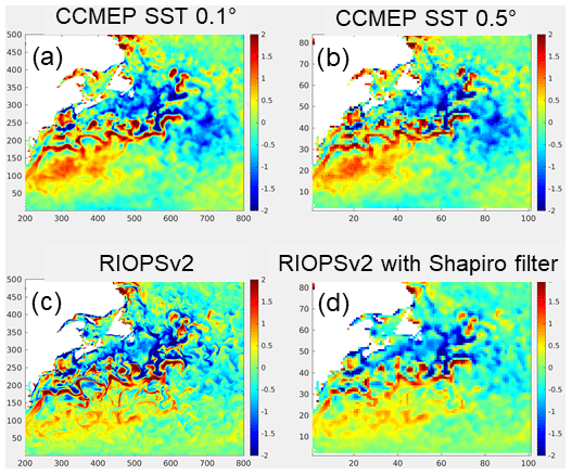
Figure 4 Example illustrating the SST filtering made as part of the observation operator in RIOPSv2 for 20 July 2016. The CCMEP SST analysis assimilated by RIOPSv2 is shown on its native 0.1^∘ latitude–longitude grid in panel (a). This analysis is first decimated to 1 point out of 5 to reduce correlated errors (b). The RIOPSv2 7 d trial field is shown in panel (c). Finally, the trial field following application of a Shapiro filter is shown in panel (d). The innovation is calculated as panel (b) minus (d).

3.4 Online harmonic analysis

Here we introduce a new online harmonic analysis method that uses a sliding-window approach to update harmonic coefficients. This approach provides an accurate estimate of tidal variability with a relatively low computational cost. Our scheme is similar to other harmonic analysis approaches (e.g., T_Tide; Pawlowicz et al., 2002) in that it is based on a least-square fit of the SSH time series by a set of harmonic functions. Here we adapt this method for efficient online model computation using a sliding-window approach with a given time weight to allow harmonic coefficients to vary in time. A detailed description of the method is given below, including a derivation of the basic harmonic analysis equations (Sect. 3.4.1) and the use of a rotation operator for the sliding-window approach (Sect. 3.4.2). A discussion of the numerical advantages of the sliding-window approach is presented in Sect. 3.4.3. Finally, the implementation details are provided in Sect. 3.4.4, together with an example showing the results of the method compared to a standard offline tidal filter. The derivation of the real-space equations implemented in NEMO for RIOPSv2 is provided in Appendix A.

3.4.1 Basic description

Given the model SSH time series Hⁿ at the nth model time step at a particular point on the model two-dimensional grid, we aim to find the harmonic spectrum coefficient X^k for each kth frequency to provide the harmonic decomposition:

$$\begin{array}{}\text{(1)}& A^n=E_k^n{X}^k,A^{\ast n}=E_k^{\ast n}{X}^{\ast k},\end{array}$$

where the superscript ^* indicates complex conjugate, and Aⁿ is the decomposition of the real time series Hⁿ. The harmonic function base is defined as

$$\begin{array}{}\text{(2)}& E_k^n=C_k\exp \left(i{\mathit{\omega }}_k\mathit{\tau }n\right),\end{array}$$

where C_k is a time-independent normalization constant factor, which could include the frequency-dependent initial phase term, ω_k is the kth pre-chosen harmonic frequency, and τ is the harmonic analysis time step length. Note that here we use n and m as indexes of time step and k and j as the frequency index, $k=\mathrm{0},\mathrm{1},\mathrm{2},\mathrm{\dots },K$. In the RIOPSv2 system, we select K=33 and specify ω₀=0 for the mean of time series H.

Aⁿ is found by minimizing the following cost function:

$$\begin{array}{}\text{(3a)}& {\displaystyle }J\left(X^k\right)={\displaystyle \frac{\mathrm{1}}{\mathrm{2}}}{\left(A^n-H^n\right)}^{\ast }{W}_{nm}\left(A^m-H^m\right),\text{(3b)}& {\displaystyle }={\displaystyle \frac{\mathrm{1}}{\mathrm{2}}}{\left(E_k^n{X}^k-H^n\right)}^{\ast }{W}_{nm}\left(E_j^m{X}^j-H^m\right),\end{array}$$

where W_nm is a real diagonal matrix of the time weights used in the sliding window; the indexes n and m take values from $-N+\mathrm{1},\mathrm{\dots },-\mathrm{2},-\mathrm{1},\mathrm{0}$, where n=0 indicates the current step. N is the sliding-window length in units of model time steps and increases with model integration time. Here, we follow the Einstein summation convention, i.e., summing over the covariant and contravariant index pairs, unless noted otherwise.

According to Eq. (3b), the variation of J on X^*k has

$$\begin{array}{}\text{(4)}& \begin{array}{rl}{\displaystyle \frac{\mathit{\delta }J}{\mathit{\delta }{X}^{\ast k}}}=& E_k^{\ast n}{W}_{nm}\left(E_j^m{X}^j-H^m\right)=\left(E_k^{\ast n}{W}_{nm}{E}_j^m\right)X^j\\ & -E_k^{\ast n}{W}_{nm}{H}^m.\end{array}\end{array}$$

We denote $B_{kj}=E_k^{*n}{W}_{nm}{E}_j^m$ with size $(K+\mathrm{1})\times (K+\mathrm{1})$ and $Y_k=E_k^{*n}{W}_{nm}{\mathbf{H}}^m$ with size $(K+\mathrm{1})\times \mathrm{1}$. If we set Eq. (4) to be equal to zero, we can obtain the minimization solution of J as follows:

$$\begin{array}{}\text{(5)}& X^j={\left({\mathbf{B}}^{-\mathrm{1}}\right)}_k^j{Y}^k,\end{array}$$

where B⁻¹ is the inverse matrix of B. Hence, we can obtain the final solution of the tidal harmonic analysis as

$$\begin{array}{}\text{(6a)}& A^n=E_j^n{\left({\mathbf{B}}^{-\mathrm{1}}\right)}_k^j{Y}^k.\end{array}$$

Note that the diagonal matrix W guarantees that matrix B is Hermitian and J is real. From Eq. (6a) we can see that the constant C in $E_k^n$ (Eq. 2) can be canceled, which means the final solution A is independent of C. Therefore, we set C=1 without any loss of generality. A convenient feature of this approach when implemented as an online harmonic analysis in a numerical model is that we only need the value of A⁰ from the current time step. Following Eq. (2), $E_j^{\mathrm{0}}$ is equal to 1 so that we have

$$\begin{array}{}\text{(6b)}& A^{\mathrm{0}}={\sum }_{j=\mathrm{0}}^K\left[{\left({\mathbf{B}}^{-\mathrm{1}}\right)}_k^j{Y}^k\right].\end{array}$$

Note that the mean of time series H is included in the above A⁰.

3.4.2 Sliding-window approach

In the following, we will show how to use a rotation operator and a sliding-window approach to update the B and Y matrices for the current time step based on previous time steps B^′ and Y^′ (hereafter, the symbol ^′ indicates the previous time step).

First, we split the summation index range of n (and m) into two sets, one for the current time step containing only step index 0 and another set for previous steps containing indexes $-N+\mathrm{1},\mathrm{\dots },-\mathrm{2},-\mathrm{1}$; to differentiate, we will use indices p and q for the latter set. Therefore, considering that W is a diagonal matrix, we can rewrite the B and Y matrices as follows:

$$\begin{array}{}\text{(7a)}& {\displaystyle }{B}_{kj}=E_k^{\ast n}{W}_{nm}{E}_j^m=E_k^{\ast \mathrm{0}}{W}_{\mathrm{00}}{E}_j^{\mathrm{0}}+E_k^{\ast p}{W}_{pq}{E}_j^q,\text{(7b)}& {\displaystyle }{Y}_k=E_k^{\ast n}{W}_{nm}{H}^m=E_k^{\ast \mathrm{0}}{W}_{\mathrm{00}}{H}^{\mathrm{0}}+E_k^{\ast p}{W}_{pq}{H}^q.\end{array}$$

According to Eq. (2), $E_k^{\mathrm{0}}$ and $E_k^{*\mathrm{0}}$ are simply equal to 1. If we denote W₀₀ as α, which is specified as the ratio of time step length τ to a given restoring time length (e.g., 30 d in RIOPSv2; see Sect. 3.4.4 for discussion), then the first terms on the right-hand side (RHS) of Eq. (7a) and (7b) become α1_kj and αV_kH⁰; here 1_kj and V_k are a matrix and a vector, respectively, with all elements equal to real number 1. In the second term on the RHS of Eq. (7b), we use n (or m) to replace p+1 (or q+1) and denote ${\mathbf{H}}^q={H^{\prime }}^m$. Here, ${H^{\prime }}^m$ is the variable H at the mth time step referred to in the previous time step.

The sliding-window weight W can then be specified as a decreasing exponential function as follows:

$$\begin{array}{ll}{\displaystyle }& {\displaystyle }{W}_{-\mathrm{1},-\mathrm{1}}=(\mathrm{1}-\mathit{\alpha })W_{\mathrm{00}},\\ {\displaystyle }& {\displaystyle }{W}_{-\mathrm{2},-\mathrm{2}}=(\mathrm{1}-\mathit{\alpha })W_{-\mathrm{1},-\mathrm{1}},\mathrm{\dots }\\ {\displaystyle }& {\displaystyle }{W}_{n-\mathrm{1},m-\mathrm{1}}=(\mathrm{1}-\mathit{\alpha })W_{nm}.\end{array}$$

In other words, $W_{pq}=(\mathrm{1}-\mathit{\alpha })W_{nm}$. As such, the second term on the RHS of Eq. (7b) can be rewritten as

$$\begin{array}{}\text{(8)}& \begin{array}{rl}& E_k^{\ast p}{W}_{pq}{H}^q={\sum }_{p,q=-N+\mathrm{1}}^{-\mathrm{1}}{E}_k^{\ast p}{W}_{pq}{H}^q\\ & =\exp \left(i{\mathit{\omega }}_k\mathit{\tau }\right){\sum }_{p,q=-N+\mathrm{1}}^{-\mathrm{1}}\exp (-i{\mathit{\omega }}_k\mathit{\tau })E_k^{\ast p}{W}_{pq}{H}^q\\ & =\exp \left(i{\mathit{\omega }}_k\mathit{\tau }\right){\sum }_{p,q=-N+\mathrm{1}}^{-\mathrm{1}}{E}_k^{\ast p+\mathrm{1}}{W}_{pq}{H}^q\\ & =\exp \left(i{\mathit{\omega }}_k\mathit{\tau }\right){\sum }_{n,m=-N+\mathrm{2}}^{\mathrm{0}}{E}_k^{\ast n}(\mathrm{1}-\mathit{\alpha })W_{nm}{H^{\prime }}^m\\ & =\left(\mathrm{1}-\mathit{\alpha }\right)\exp \left(i{\mathit{\omega }}_k\mathit{\tau }\right){\sum }_{n,m=-N+\mathrm{1}}^{\mathrm{0}}{E}_k^{\ast n}{W}_{nm}{H^{\prime }}^m\\ & +O\left(W_{-N+\mathrm{1},-N+\mathrm{1}}\right)\\ & =\left(\mathrm{1}-\mathit{\alpha }\right)\exp \left(i{\mathit{\omega }}_k\mathit{\tau }\right)Y_k^{\prime }+O\left(W_{-N+\mathrm{1},-N+\mathrm{1}}\right).\end{array}\end{array}$$

Here, the term $O\left(W_{-N+\mathrm{1},-N+\mathrm{1}}\right)$ results from the change in the lower limit of the summation of n(m) from $-N+\mathrm{2}$ to $-N+\mathrm{1}$. Generally speaking, this term can be neglected when N is sufficiently large because $W_{-N+\mathrm{1},-N+\mathrm{1}}$ is very small, on the order of $(\mathrm{1}-\mathit{\alpha }{)}^{N-\mathrm{1}}$ and $\mathit{\alpha }(\mathrm{1}-\mathit{\alpha }{)}^{N-\mathrm{1}}$ compared with W₀₀ and Y, respectively. For example, in RIOPS with a 30 d restoring time length and after a half-year spin-up period, they are about $e^{-\mathrm{6}}=\mathrm{2.479}\times {\mathrm{10}}^{-\mathrm{3}}$ and $\mathrm{1}/(\mathrm{288}\cdot \mathrm{30})\cdot e^{-\mathrm{6}}=\mathrm{2.869}\times {\mathrm{10}}^{-\mathrm{7}}$, respectively.

Therefore, using Eqs. (8) and (7b), we can obtain

$$\begin{array}{}\text{(9)}& Y_k=\mathit{\alpha }{\mathit{V}}_k{H}^{\mathrm{0}}+(\mathrm{1}-\mathit{\alpha })R_k^{\ast j}{Y^{\prime }}_j,\end{array}$$

where R is a diagonal time-independent rotation matrix, with its kth diagonal element taking the value

$$\begin{array}{}\text{(10)}& R_k^k=\exp (-i{\mathit{\omega }}_k\mathit{\tau }).\end{array}$$

The matrix R can be used to rotate a complex vector in the complex plane spanned by the kth complex harmonic function base. For instance, a complex vector e^iθ could be rotated into a vector $e^{i(\mathit{\theta }-{\mathit{\omega }}_k\mathit{\tau })}$ by operator $R_k^k$. One exception is that when ω₀=0, as is the case for the mean of time series of Hⁿ, both $R_{\mathrm{0}}^{\mathrm{0}}$ and $E_{\mathrm{0}}^n$ are equal to the real number 1 so that there is no complex plane spanned, and R only takes action in the one-dimensional real space. Similarly, we can rewrite the RHS of Eq. (7a) as

$$\begin{array}{}\text{(11a)}& \begin{array}{rl}& E_k^{\ast p}{W}_{pq}{E}_j^q={\sum }_{p,q=-N+\mathrm{1}}^{-\mathrm{1}}{E}_k^{\ast p}{W}_{pq}{E}_j^q\\ & =\exp \left(i{\mathit{\omega }}_k\mathit{\tau }\right)\exp (-i{\mathit{\omega }}_j\mathit{\tau }){\sum }_{p,q=-N+\mathrm{1}}^{-\mathrm{1}}\\ & \exp \left(-i{\mathit{\omega }}_k\mathit{\tau }\right)E_k^{\ast p}{W}_{pq}{E}_j^q\exp \left(i{\mathit{\omega }}_j\mathit{\tau }\right)\\ & =\exp \left(i{\mathit{\omega }}_k\mathit{\tau }\right)\exp (-i{\mathit{\omega }}_j\mathit{\tau }){\sum }_{p,q=-N+\mathrm{1}}^{-\mathrm{1}}\\ & E_k^{\ast p+\mathrm{1}}{W}_{pq}{E}_j^{q+\mathrm{1}}\\ & =\exp \left(i{\mathit{\omega }}_k\mathit{\tau }\right)\exp (-i{\mathit{\omega }}_j\mathit{\tau }){\sum }_{n,m=-N+\mathrm{2}}^{\mathrm{0}}\\ & E_k^{\ast n}(\mathrm{1}-\mathit{\alpha })W_{nm}{E}_j^m\\ & =\left(\mathrm{1}-\mathit{\alpha }\right)\exp \left(i{\mathit{\omega }}_k\mathit{\tau }\right)\exp (-i{\mathit{\omega }}_j\mathit{\tau }){\sum }_{n,m=-N+\mathrm{1}}^{\mathrm{0}}\\ & E_k^{\ast n}{W}_{nm}{E}_j^m+O\left(W_{-N+\mathrm{1},-N+\mathrm{1}}\right)\\ & =\left(\mathrm{1}-\mathit{\alpha }\right)\exp \left(i{\mathit{\omega }}_k\mathit{\tau }\right)B_{kj}^{\prime }\exp (-i{\mathit{\omega }}_j\mathit{\tau })\\ & +O\left(W_{-N+\mathrm{1},-N+\mathrm{1}}\right)\\ & =\left(\mathrm{1}-\mathit{\alpha }\right){\mathrm{R}}_k^{\ast i}{B}_{il}^{\prime }{\mathrm{R}}_j^l+O\left(W_{-N+\mathrm{1},-N+\mathrm{1}}\right).\end{array}\end{array}$$

Combining Eqs. (7a) and (11a), we can write

$$\begin{array}{}\text{(11b)}& B_{kj}=\mathit{\alpha }{\mathrm{1}}_{kj}+(\mathrm{1}-\mathit{\alpha })R_k^{\ast i}{B^{\prime }}_{il}{R}_j^l.\end{array}$$

Finally, based on Eqs. (6b) and (9)–(11b), we can get the final solution A⁰ for the current time step. Appendix A provides the derivation of the equivalent real-space version of these equations that is coded in RIOPSv2.

3.4.3 Numerical advantages

The main advantage of this sliding-window approach is that it is much cheaper to use than the traditional method. For instance, in RIOPSv2 the number of horizontal grid points is $N_{xy}=\mathrm{1580}\times \mathrm{2198}$, and if we update tidal harmonics at each model step with a half-year spin-up window (or analysis time window), this implies a total number of time steps of $N_{\mathrm{stp}}=\mathrm{288}\times \mathrm{182}$. This means the size of Y is less than 2 GB ($\sim \mathrm{8}\times N_{xy}\times (\mathrm{2}K+\mathrm{1})$) for our method and over 1 TB ($\sim \mathrm{8}\times N_{xy}\times N_{\mathrm{stp}}$) for the traditional method. In addition, updating Y at each model time step using the traditional method by equation $Y_k=E_k^{*n}{W}_{nm}{H}^m$ would require the computation of sine and cosine decomposition operators $N_{xy}\times (\mathrm{2}K+\mathrm{1})\times N_{\mathrm{stp}}$ times. Alternatively, the method outlined here requires only the use of the multiplication operator $N_{xy}\times (\mathrm{2}K+\mathrm{1})$ times. Moreover, to speed up computation in the traditional method one could save the sine and cosine decomposed values at each model step; however, the data size of Y will become huge, over 2K+1 TB. As such, the traditional method would be too slow for operational systems based on the present-day computing environments unless one made some modifications and/or simplifications. For instance, the cost could be lowered by reducing the resolution of the temporal and the spatial calculations. However, this could have negative consequences in coastal areas and areas of steep bathymetric slope as the local geometric structures have a strong influence on the tidal harmonics, as do high-frequency tidal constituents.

As we assume that the matrix B is homogeneous for the horizontal grids, the data size is very small $\left(\right(K+\mathrm{1})\times (K+\mathrm{1})$ in complex and $(\mathrm{2}K+\mathrm{1})\times (\mathrm{2}K+\mathrm{1})$ in real space, respectively), and there is no issue for B regarding differences of computational costs, memory, and I/O between the traditional method and online harmonic analysis with the sliding window.

Another advantage of the sliding-window approach is with respect to its spin-up. As we know, dynamic models and data assimilation systems require a certain time period to be spun up to equilibrium. When applying the online tidal harmonic analyses, we can allow all three parts (model, assimilation, and tidal filter) to be coupled in harmony during the common spin-up time window from the model cold start.

3.4.4 Implementation details

This sliding-window approach is implemented using the real-space version of the equations (Appendix A) such that Eqs. (A2)–(A4) are updated at every time step using 33 diurnal and semi-diurnal tidal constituents. Updating these equations less frequently (e.g., every four model time steps or hourly) was found to have a negative impact on the accuracy of the harmonic analysis and resulted in an increase in the tidal energy remaining in the SSH residual. The choice of 33 tidal constituents was based on the results of an offline harmonic analysis made using T_tide (Pawlowicz et al., 2002). Additionally, no harmonics with a period longer than 30 h were used to avoid contamination of the tidal signal by mesoscale variability.

The other free parameter in the sliding-window approach is the timescale used in the weighting function. Here a value of 30 d is used. This value must be large enough to permit an accurate fit of the different tidal constituents. Using a longer value reduces the ability of the system to adapt to seasonal (or longer) changes in tidal variability.

A comparison between the online harmonic approach and the well-known T_tide package is provided in Fig. 5. The unfiltered SSH and tidal residuals using both the online approach introduced here and T_tide are shown for a point in Ungava Bay (location indicated by a star in Fig. 6). This region is characterized by extremely large tidal amplitudes and seasonal ice cover. From Fig. 5 we can see that while both approaches provide similar tidal residuals (Fig. 5b), instantaneous differences of up to 0.5 cm may be present. This value corresponds to roughly 20 % of the observational error used for some satellite altimeters. Moreover, Fig. 5d shows that the amplitude of the high-frequency tidal variations in the tidal residual is larger for T_tide. While the period of analysis is too short to be conclusive, there does appear to be a seasonal cycle in the amplitude of the differences in tidal residuals (Fig. 5c), with larger differences in winter months potentially due to the presence of sea ice.

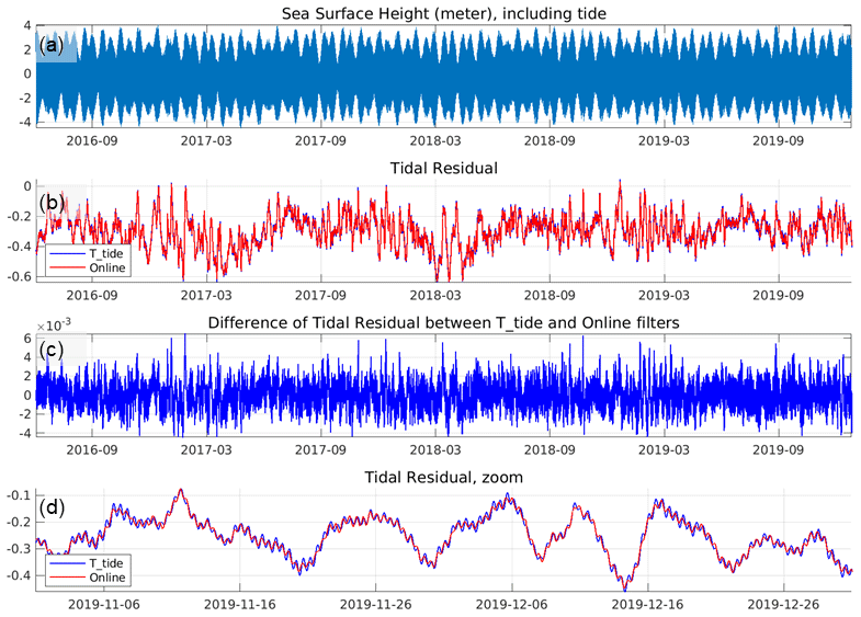
Figure 5 Example illustrating the performance of the online harmonic analysis compared to the T_tide offline filter for a location in Ungava Bay (location shown with a star in Fig. 6). Unfiltered sea surface height (SSH) variations (in meters) are shown in panel (a). The residual SSH variability following removal of the tidal signal using the T_tide package (blue line) and the online harmonic analysis (red line) is shown in panel (b). The difference between the two residuals is shown in panel (c). Panel (d) provides a subsample (zoom) of the results from panel (b) over a roughly 2-month period.

To illustrate the relative importance of the various filtering steps, the different components (tides, inverse barometer) have been separated and an example is shown in Fig. 6. The tidal signal is the most prominent source of variability and has a significant impact, with local variations exceeding 1 m in amplitude. In comparison, the inverse barometer effect is generally below 0.2 m. The residual SSH with tides and inverse barometer removed shows the main physical features well, including the Gulf Stream and Beaufort Gyre. Some tidal variability remains in coastal areas with strong tides (e.g., Bay of Fundy), but this is expected to have a negligible effect as SLA observation errors are amplified nearshore to account for representativity error.

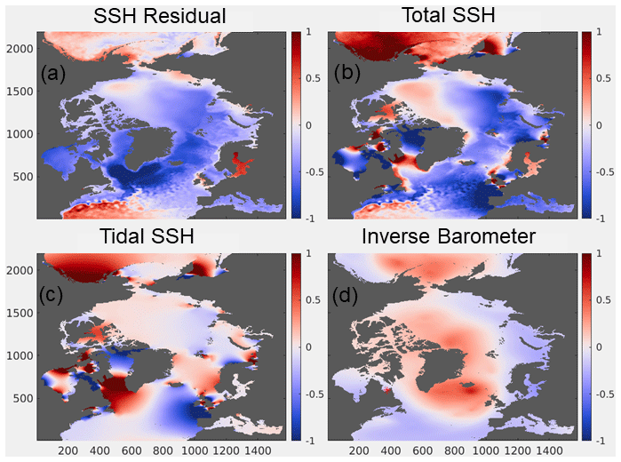
Figure 6 Example showing the impact of tidal and inverse barometer terms on the SLA observation operator for 31 December 2015. The SSH residual used in the SLA observation operator is shown in panel (a). Panel (b) shows the instantaneous model SSH field prior to any treatment. The tidal component calculated using the online harmonic analysis is shown in panel (c). Panel (d) shows the inverse barometer component. Units are meters (m). Fields are plotted on the native model grid with grid point numbers shown on the x and y axes. The SST residual (a) is calculated as the total SSH field (b) minus the tidal SSH (c) and the inverse barometer term (d).

4 Evaluation

The evaluation of RIOPSv2 will be made in three parts. First, an evaluation of the innovations (model minus observation differences) will be presented for both RIOPSv2 and GIOPSv3 to demonstrate that the adaptations of SAM2 for the RIOPSv2 system are performing well and to highlight the areas of improvement and degraded performance. We then assess the variations in sea level anomaly along a particular Jason satellite altimetry track over the 3-year evaluation period to show specific differences in the quality of the two analysis systems. Finally, we compare the power spectral density of the kinetic energy fields to investigate the representation of smaller-scale oceanic features in the RIOPS analyses. We begin by describing the experimental setup used to produce the analysis cycles being evaluated.

4.1 Experimental setup

To support the evaluation, weekly (RD) analysis cycles were produced over a 3-year period (9 September 2015 to 2 January 2019). The simulations are initialized from rest on 9 September 2015 from the World Ocean Atlas Climatology 2013v2 (Boyer et al., 2013) temperature and salinity fields, with ice fields taken from the forced model simulation used to produce the error modes. Following 6 weeks of spin-up (i.e., six cycles), the ocean data assimilation scheme is activated. This approach allows the online harmonic analysis sufficient time to converge prior to assimilating SLA. The system is then run for 10 cycles to allow the system to stabilize and the amplitude of innovations to decrease as fields are adjusted towards current conditions. The evaluation is then performed on the subsequent cycles run from 6 January 2016 to 2 January 2019.

Atmospheric forcing is applied in the same manner as used in operations, which means using the lowest-level atmospheric forecasts fields from the Regional Deterministic Prediction System (RDPS; 10 km grid resolution) blended with fields from the Global Deterministic Prediction System (GDPS; 25 km grid resolution) to cover the full RIOPS domain (for details see Dupont et al., 2019). Forecast fields from subsequent twice-daily forecasts (i.e., at 00:00 and 12:00 Z daily) at lead times of 06:00–24:00 h are blended together with a 6 h linear interpolation window to provide a continuous atmospheric forcing set. This approach minimizes potential shocks in atmospheric pressure fields due to variations in subsequent forecasts. Note that errors found here (in particular SST biases) may be larger than found in the real-time operational RIOPSv2 due to improvements implemented in the RDPS and GDPS, in particular those associated with the use of GEMv5 (McTaggart-Cowen et al., 2019) following the implementation on 3 July 2019.

The reference simulations used here for comparison are from the GIOPSv3 system. This was chosen as a reference since it uses an equivalent ocean data assimilation system and thus provides an assessment focused on the regional adaptations introduced here for RIOPSv2. Moreover, the RIOPSv1 system constrained temperature and salinity fields towards GIOPS using a spectral nudging approach. Thus, comparison of RIOPSv2 with GIOPSv3 provides a proxy for differences between RIOPSv2 and RIOPSv1. Direct comparison of RIOPSv2 and RIOPSv1 using innovation statistics is not possible since the innovations are calculated online and RIOPSv1 did not use SAM2. The GIOPSv3 simulation used here for comparison was initialized and spun up using the exact same methodology as used for RIOPSv2. For both RIOPSv2 and GIOPSv3, the SLA observations used during the evaluation period include SARAL/AltiKa, Jason-2 (until September 2016), Jason-2N (from February to June 2017), Jason-3 (from September 2016 onwards), and CryoSat-2. With at least three radar altimeters working at any given time, this provides a fairly data-rich period for SLA with which to evaluate the assimilation system.

4.2 Innovations

Here we present innovation statistics calculated over the 3-year evaluation period for SLA, SST, and temperature and salinity profile data. As noted in Sect. 3.1, SAM2 uses an FGAT approach to calculate innovations at the closest model time step. To provide a spatial representation of the innovation statistics, innovations were binned on a 1^∘ latitude–longitude grid. The mean and root mean squared (rms) differences were then produced for each evaluation grid point for innovations covering the full 3-year period. For profile data, innovations were evaluated over different depth ranges. For brevity, here we show results over the depth ranges 0–500 and 500–2000 m.

4.2.1 SLA innovations

The mean and rms innovation statistics for SLA are shown in Fig. 7. The largest innovations for both RIOPSv2 and GIOPSv3 occur over the Gulf Stream region due to the associated strong mesoscale variability. In GIOPSv3, rms differences exceed 25 cm from the east coast of North America eastward to 45^∘ W. RIOPSv2 shows notably smaller rms differences over this region, with values closer to 20 cm. These improvements are due in part to the smaller values of MDT representation error used in RIOPSv2, together with the higher model grid resolution that can better represent mesoscale structures.

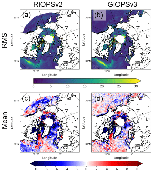
Figure 7 Innovation (observation–model) statistics of sea level anomaly for the period 1 January 2016 to 31 December 2018. The rms (a, b) and mean differences (c, d) are shown for RIOPSv2 (a, c) and GIOPSv3 (b, d).

A second region of large SLA innovations can be found in the Arctic Ocean. In the northern Laptev and Beaufort seas, rms differences larger than 20 cm are present. These regions are also characterized by negative mean SLA innovations of greater than 10 cm in GIOPSv3 and RIOPSv2. As such, the differences may be associated with the CNES-CLS13 MDT field used. As this area is typically ice-covered, the MDT would have had a few years of open-water data to use in its production. These regions are also strongly affected by freshwater drainage from the Mackenzie River and rivers in Russia that may affect the SLA. For example, a negative SLA bias of 10 cm (positive values in Fig. 7c and d) at the mouth of the Lena River (135^∘ W) is likely due to positive anomalies in actual river runoff compared to the climatological values used here by both systems. Note also that due to satellite orbits and ice coverage, far fewer observations are present over the Arctic Ocean, with fewer than 500 measurements per bin compared to over 2000 measurements per bin south of 66^∘ N. As such, the statistics over the Arctic are less reliable and more seasonally dependent.

Finally, a region with slightly increased rms differences in RIOPSv2 is noted in Hudson Bay and the northern Labrador Sea. These regions show larger rms differences of up to 5 cm and are likely associated with residual tidal variability remaining after application of the online harmonic analysis due to fortnightly and monthly timescale tidal harmonics.

4.2.2 SST innovations

SST innovations between RIOPSv2 and GIOPSv3 are broadly similar (Fig. 8), with the largest errors occurring in the Gulf Stream and along the winter marginal ice zone in the Labrador Sea and Greenland–Iceland–Norwegian seas. The rms SST innovations in the Gulf Stream region decrease from upwards of 2.0 ^∘C for GIOPSv3 to around 1.5 ^∘C for RIOPSv2. The largest SST innovations for both systems occur along the tail of the Grand Banks around 45^∘ W, likely due to the presence of strong SST gradients. Along the region of maximum ice extent in winter, errors of around 0.8 ^∘C are present. In most other areas, errors in both systems are less than 0.5  ^∘C, which is the nominal error of the CCMEP SST analysis (Brasnett and Colan, 2016). Similar to innovations of SLA (Fig. 7), a slight increase in rms SST innovations in RIOPSv2 can be seen in the central Labrador Sea.

Figure 8 Innovation (observation–model) statistics of sea surface temperature for the period 1 January 2016 to 31 December 2018. The rms (a, b) and mean differences (c, d) are shown for RIOPSv2 (a, c) and GIOPSv3 (b, d).

4.2.3 $T/S$ profile innovations

Innovation statistics obtained from in situ temperature and salinity profiles averaged over the upper 500 m of the water column and over the range 500–2000 m are shown in Figs. 9–11. These observations are composed mainly of data from Argo profiling floats, with some additional profiles from field campaigns, moorings, voluntary observing ships, gliders, and marine mammals. Interestingly, the period of evaluation includes the Year of Polar Prediction (YOPP; Jung et al., 2016) for which a number of additional in situ ocean observations were deployed (Smith et al., 2019b). These include Argo and ALAMO floats (Wood et al., 2018) used seasonally during ice-free periods as well as ice-tethered profilers (ITPs; Toole et al., 2011). These, together with other additional ocean observations deployed during YOPP, provide an exceptional opportunity to evaluate water mass properties in RIOPS and GIOPS over the Arctic Ocean, for which a significant gap is usually present in the in situ ocean observing network.

As shown for SLA and SST, the largest innovations in profile data for both systems are found in the Gulf Stream region due to the strong mesoscale variability and important spatial variability in water mass properties (Figs. 9 and 11). Significant innovations in salinity are also found along many coastal regions. On the Canadian east coast, in the Gulf of St. Lawrence, and along the Labrador Coast, rms salinity innovations often exceeding 0.5 psu are present. Similar errors are present around the North Sea and along the Norwegian coastline, with slightly larger values in RIOPSv2. The larger biases in RIOPSv2 may be associated with a positive salinity bias in the upper 50 m of the water column (not shown). This bias may be due to a deficit in river runoff together with the associated reduction in vertical stratification, resulting in overly intense vertical mixing due to tides.

Figure 9 Innovation (observation–model) statistics of in situ temperature and salinity over the upper 500 m depths for the period 1 January 2016 to 31 December 2018. The rms differences for temperature (a, b) and salinity (c, d) are shown for RIOPSv2 (a, c) and GIOPSv3 (b, d).

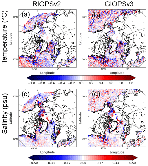
Figure 10 Innovation (observation–model) statistics of in situ temperature and salinity over the upper 500 m depths for the period 1 January 2016 to 31 December 2018. The mean differences for temperature (a, b) and salinity (c, d) are shown for RIOPSv2 (a, c) and GIOPSv3 (b, d).

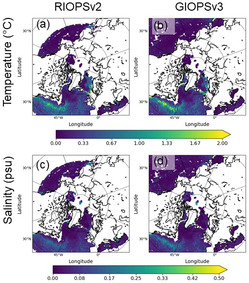
Figure 11 Innovation (observation–model) statistics of in situ temperature and salinity over the depth range 500–2000 m for the period 1 January 2016 to 31 December 2018. The rms differences for temperature (a, b) and salinity (c, d) are shown for RIOPSv2 (a, c) and GIOPSv3 (b, d).

The Arctic observations are quite revealing, highlighting important positive biases in salinity (i.e., too salty) in the Beaufort Sea (Fig. 10c) associated with the halocline (centered at 50 m of depth) and Pacific water layer (200–300 m of depth; not shown). This bias is smaller in GIOPSv3 in the eastern Beaufort Sea, with a salinity bias of less than 0.2 psu, whereas RIOPSv2 shows values up to 0.4 psu. The source of this bias is under investigation and will be part of a study to investigate how to better constrain water masses in the Arctic using observations from YOPP.

Errors in other regions are generally quite small in both systems. In the Pacific Ocean, the 3D-Var bias correction scheme considerably reduces the biases in salinity over the upper 500 m. Without the bias correction scheme, errors of up to 0.5 psu occur over a broad region in the North Pacific Ocean along the Aleutian Islands (not shown).

4.2.4 Evaluation of sea level anomalies over the Gulf Stream region

As the Gulf Stream region shows the largest rms innovation errors for all fields, we now focus on a comparison of SLA anomalies and resolved spatial scales over this region. Figure 12 shows Hovmöller diagrams for a particular Jason altimeter track, illustrating the evolution of SLA anomalies over the evaluation period. The vertical axis is constructed using the SLA anomalies over the track from the 10 d repeat orbit with each row representing one track. The location of the track is shown in green in Fig. 12b. Both RIOPSv2 and GIOPSv3 capture the low-frequency variations in SLA due to the evolution of mesoscale ocean features in this highly dynamic region. Indeed, SLA variations are present with a range greater than 1 m, yet rms differences for RIOPSv2 and GIOPSv3 are only 12 and 14 cm, respectively (Table 3). Differences between the analysis system and the observations (Fig. 12d and f) tend to be quite localized in time. The differences occur less frequently in RIOPSv2, suggesting a better representation of the mesoscale eddy field. In addition, GIOPS shows a significant period of error related to a negative SLA anomaly that occurred around 62^∘ W in mid-2017. The closer fit of RIOPS to observations is reflected in higher correlations and lower rms error between RIOPS and the SLA observations (Table 3).

Table 3 SLA statistics for GIOPSv3 and RIOPSv2 compared to a particular Jason satellite altimetry track across the Gulf Stream (shown in Fig. 12b).

Figure 12 Hovmöller diagrams showing variations in sea level anomaly (SLA; units are meters) for the period 1 January 2016 to 31 December 2018 along a repeat altimeter track of the Jason altimeter (green line in panel b, units are kilometers). Observations prior to 7 September 2016 are taken from Jason-2, and Jason-3 is used thereafter. Satellite observed values are shown in panel (a) along with values for RIOPSv2 (c) and GIOPSv3 (e). Differences (obs – model) for RIOPSv2 and GIOPSv3 are shown in panels (d) and (f), respectively. Periods of missing observations are shown as grey boxes.

Given the higher spatial resolution of RIOPSv2, one would expect to see finer scales present in the details of the along-track SLA anomalies. As this is not obvious from Fig. 12 we will now investigate the power spectral density (PSD) of the surface kinetic energy (KE) fields from RIOPSv2 and GIOPSv3 over the Gulf Stream region (Fig. 13) following the approach of Jacobs et al. (2019). First, we compute the Fourier transform of both zonal and meridional surface current fields over a box covering the Gulf Stream region (48.8–66.0^∘ W, 32.3–45.0^∘ N) using weekly instantaneous SLA fields from both RIOPSv2 and GIOPSv3 over the full 3-year evaluation period. The results are then averaged in time and between velocity components to provide the PSD of KE.

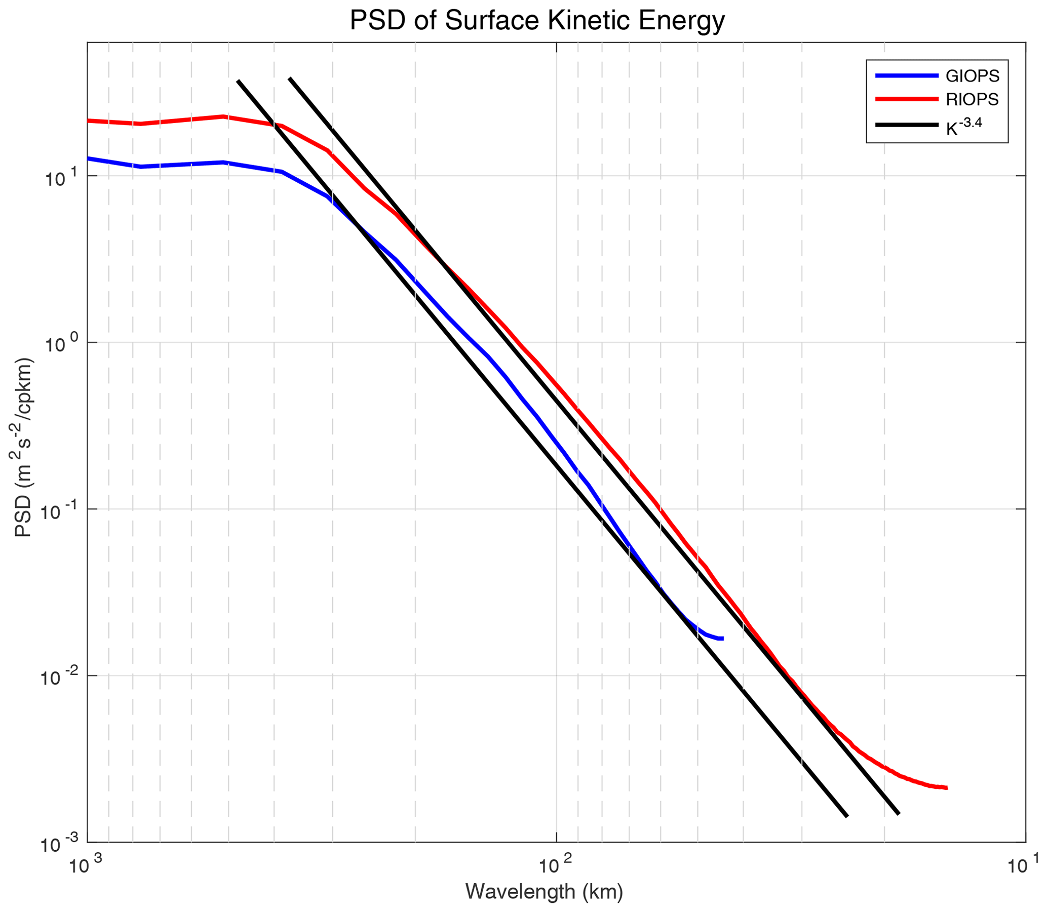
Figure 13 Power spectral density (PSD) of the surface kinetic energy in RIOPSv2 (red line) and GIOPSv3 (blue line). The PSD is calculated using both zonal and meridional surface current fields over a box covering the Gulf Stream region (48.8–66.0^∘ W, 32.3–45.0^∘ N) using weekly instantaneous SLA fields over the period 1 January 2016 to 31 December 2018. The k^−3.4 line is shown in black and adjusted to fit the curves for RIOPSv2 and GIOPSv3. The wavelengths at which the PSD curves depart from the k^−3.4 line are shown for both the high and low wavelength limits.

Overall, the surface kinetic energy for RIOPSv2 shows 1.7 times the power over the full spectrum, with higher power at all wavelengths. The PSD for both systems closely follows the k^−3.4 line over the mesoscale band, in agreement with Jacobs et al. (2019), demonstrating a good representation of the energy cascade. The wavelengths for which the PSD deviates from the k^−3.4 line at both the high and low wavelength limits are indicated in Fig. 13. Due to the higher model resolution, RIOPSv2 extends the mesoscale band down to about 35 km compared to 66 km for GIOPS. These scales provide an indication of the effective model resolution and are equivalent to roughly five and three model grid points for RIOPSv2 and GIOPSv3, respectively. The long-wavelength limits for RIOPSv2 and GIOPSv3 are broadly similar, with values of 178 and 208 km, respectively. Both systems show a peak in PSD around 416 km.

5 Summary and discussion

Here we present a description and evaluation of the first pan-Canadian ocean analysis system running operationally as part of RIOPSv2. This system includes various improvements with respect to its equivalent global ocean analysis system, GIOPSv3. These improvements include a 7 d IAU procedure, the use of higher-resolution background error modes, and a spatial filter used as part of the sea surface temperature observation operator. The most notable change, however, is the inclusion of tides, which requires an online harmonic analysis of sea surface height as part of the observation operator. A new method is presented here that makes use of a sliding-window approach. This approach allows for time-varying harmonic constants that can adapt to seasonal variations in the tides due to the sea ice cover (e.g., Kleptsova and Pietrzak, 2018).

An evaluation is presented of innovations of SLA, SST, and in situ temperature and salinity profile observations for RIOPSv2 and GIOPSv3 over a 3-year period. The results show similar overall innovation statistics between the two systems, demonstrating that the use of explicit tides and the online tidal filter do not lead to any significant degradation in the quality of the analyses. The largest errors for both systems occur in the Gulf Stream region for all fields, with smaller rms innovations for RIOPSv2 of about 5 cm for SLA and 0.5 ^∘C for SST.

Some areas do show larger innovation statistics for RIOPSv2, highlighting areas for improvement. In the Arctic Ocean, larger mean and rms SLA errors are found for RIOPSv2 close to the North Pole in the marginal ice zone of the seasonal sea ice minimum. These errors may be related to errors in the CNES-CLS13 MDT as significant mean innovations are present and fewer observations were available to construct the MDT in these regions. These errors in the central Arctic may be expected to occur more frequently in the real-time operational systems in future years, as declining summer sea ice cover in the Arctic will lead to increasing areas of open water.

Some increases in SLA innovations (up to 5 cm) locally in areas of Hudson Bay and Baffin Bay are also found. As these regions experience strong tides with important seasonality and baroclinic effects (Saucier et al., 2004), the increase in SLA innovation statistics may be due to unfiltered tidal residuals related to fortnightly baroclinic modes. Extending the online tidal filter approach from a 1D analysis to take into account 2D tidal correlations may be able to improve this somewhat by making it possible to increase the number of constituents (i.e., to include fortnightly and monthly) without erroneously filtering mesoscale variability.

As part of YOPP (2017–2019), a significant number of in situ temperature and salinity observations were taken and made available via the Global Telecommunications System, allowing their use in studies such as these that rely on operational databases. These valuable observations provide a rare glimpse at errors in Arctic water mass properties (Smith et al., 2019b). Here, we see RIOPSv2 shows larger salinity errors in the Beaufort Sea, with mean salinity biases over the upper 500 m of 0.3–0.4 psu in the eastern Beaufort Sea. Larger salinity biases are also present along many coastlines for RIOPSv2, in particular in the Baltic and North seas.

As the largest innovations in both RIOPSv2 and GIOPSv3 occur in the Gulf Stream region, a comparison of SLA along a particular Jason satellite track was made. Both systems capture the main evolution of mesoscale variations; however, RIOPSv2 shows smaller differences from SLA observations than GIOPSv3 (Table 3), with higher correlation (0.82 and 0.73, respectively) and lower rms (12 and 14 cm, respectively).

To investigate the role of increased resolution in RIOPSv2, the PSD of surface kinetic energy over the Gulf Stream region was investigated. The PSD of RIOPSv2 is 1.7 times the power of GIOPSv3 and contains smaller scales down to roughly 35 km compared to 66 km for GIOPSv3. These scales give an indication of the effective model resolution and roughly correspond to five and three grid points, respectively. These values are somewhat smaller than one would expect purely from a numerical point of view (generally the smallest feature resolvable requires 6–10 grid points) and suggest that the data assimilation may be artificially increasing the resolution somewhat. This is not surprising for GIOPSv3, as it has only a $\mathrm{1}/\mathrm{4}$^∘ grid resolution and is thus considered eddy-permitting only.

The evaluation presented here demonstrates that RIOPSv2 is able to produce analyses of a similar quality as GIOPSv3 albeit including higher grid resolution and explicit tides. However, the evaluation is restricted to the observations assimilated by the systems and provides only indirect information regarding the quality of related quantities such as surface currents, which are important for key applications of RIOPSv2 like emergency response. An alternative means to evaluate the skill of surface currents is to use drifting buoys. A significant effort is underway as part of the Ocean Protection Plan initiative by the Canadian government to deploy various types of drifters in Canadian waters to evaluate numerical ocean predictions. As part of this effort, a comparison of RIOPSv1.3 and TOPAZ with drifter observations off the coast of Norway showed positive results (Sutherland et al., 2020).

Despite being an important application for RIOPSv2, quantitative evaluation for emergency response is especially challenging due to a lack of cases with sufficient data. Qualitative evaluations from respondents from the emergency response section at CCMEP have found that RIOPSv2 provides significant improvements in many areas. However, in cases close to the coast, RIOPSv2 applicability is limited due to the relatively coarse ∼ 3–6 km grid along the Canadian coastline. As a result, two sub-domains at 2 km grid resolution that downscale RIOPSv2 fields have been developed and are being run experimentally at CCMEP to evaluate the added value of increased resolution. An evaluation of RIOPSv2 analyses for the Canadian east and west coasts is being made as part of this effort that includes comparison with drifting buoys, acoustic Doppler current profiler observations, and high-frequency radar observations.

Another important application of RIOPSv2 is for sea ice prediction. An evaluation of forecasts of sea ice concentration, drift, and thickness showed very little change from RIOPSv1.3 to RIOPSv2 (Dupont et al., 2019). The only significant impact is a slight reduction in the negative bias in ice drift due to the reduction in the ice–ocean drag coefficient. The lack of impact on sea ice is not surprising given the similarity between RIOPSv2 and GIOPSv3 analyses and the fact that RIOPSv1.3 used a spectral nudging approach toward GIOPS analyses. As such, differences in ocean fields (e.g., SST, mixed-layer depth) in the vicinity of the sea ice were quite small and thus had little impact on the evolution of sea ice fields (e.g., due to formation and melt).

Appendix A: Derivation of real-space equations for the sliding-window online harmonic analysis

In RIOPSv2, we work on the real vector space spanned by the real function base pair of cos (ω_kτn) and sin (ω_kτn). To replace the complex space spanned by $e^{i{\mathit{\omega }}_k\mathit{\tau }n}$ as described in Sect. 3.4.2 we employ the Euler identity ${\mathit{e}}^{i\mathit{\theta }}=\cos \mathit{\theta }+i\sin \mathit{\theta }$. Its dimension becomes $\mathrm{2}K+\mathrm{1},$ including the one-dimensional real subspace for ω₀=0. The complex space matrices R and B are replaced by real-space matrix S and D with size $(\mathrm{2}K+\mathrm{1})\times (\mathrm{2}K+\mathrm{1})$, respectively. Similarly, complex space vector Y is replaced by real-space vector Z with size (2K+1)x1. This is just a transform of the operators' representative space from complex space to the equivalent two-dimensional (2D) real space.

Because R is a diagonal matrix in the K+1-dimensional complex space, there is no frequency mixing when operating by R. This means that each 2D real vector space is a complete invariant subspace when operating under S. In addition, when ω₀=0, it is a 1D complete invariant subspace. In other words, the 2K+1 dimensional space that S operates on is reducible, and it can be reduced into a direct-sum space of one 1D-invariant subspace and K 2D-invariant subspaces. In doing so, S would be reduced and represented as a block-diagonal matrix as follows:

$$\begin{array}{}\text{(A1)}& S=S^{\mathrm{0}}\oplus \sum _{k=\mathrm{1}}^K\oplus S^k.\end{array}$$

Here, ⊕ is the matrix direct-sum operator, S⁰ is the real number 1 for ω₀=0, and S^k is a 2D real rotation matrix with rotation angle ω_kτ. Therefore, we can rewrite Eqs. (9), (11b), and (6b) as the following 2K+1-dimensional real-space vector and matrix format:

$$\begin{array}{}\text{(A2)}& {\displaystyle }& {\displaystyle }Z=\mathit{\alpha }\mathit{U}{H}^{\mathrm{0}}+(\mathrm{1}-\mathit{\alpha }){\mathbf{S}}^{\mathrm{T}}{Z}^{\prime },\text{(A3)}& {\displaystyle }& {\displaystyle }D=\mathit{\alpha }{\mathrm{1}}_c+(\mathrm{1}-\mathit{\alpha })S^T{D}^{\prime }S,\text{(A4)}& {\displaystyle }& {\displaystyle }{A}^{\mathrm{0}}={\sum }_{\cos }\left[{\mathbf{D}}^{-\mathrm{1}}Z\right].\end{array}$$

Here, U and 1_c are a real vector and matrix with an element equal to 0 if the element involves the sine dimension; otherwise, the element is equal to 1 because both 1_kj and V_k are real number 1 in Eqs. (9) and (11b). S^T is the transpose of S, and the symbol Σ_cos denotes summing over only the cosine components of the 2K+1-dimensional vector D⁻¹Z.