the Creative Commons Attribution 4.0 License.
the Creative Commons Attribution 4.0 License.
 | 24 Feb 2021
A fully coupled Arctic sea-ice–ocean–atmosphere model (ArcIOAM v1.0) based on C-Coupler2: model description and preliminary results
Shihe Ren
Qizhen Sun
L. Bruno Tremblay
Bo Lin
Xiaoping Mai
Fu Zhao
Na Liu
Zhikun Chen
Yunfei Zhang
The Arctic regional coupled sea-ice–ocean–atmosphere model (ArcIOAM) has been developed to provide reliable Arctic sea ice prediction on seasonal timescales. The description and implementation of ArcIOAM and its preliminary results for the year of 2012 are presented in this paper. In the ArcIOAM configuration, the Community Coupler 2 (C-Coupler2) is used to couple the Arctic sea-ice–oceanic configuration of the MITgcm (Massachusetts Institute of Technology general circulation model) with the Arctic atmospheric configuration of the Polar WRF (Weather Research and Forecasting) model. A scalability test is performed to investigate the parallelization of the coupled model. As the first step toward reliable Arctic seasonal sea ice prediction, ArcIOAM, implemented with two-way coupling strategy along with one-way coupling strategy, is evaluated with respect to available observational data and reanalysis products for the year of 2012. A stand-alone MITgcm run with prescribed atmospheric forcing is performed for reference. From the comparison, all the experiments simulate reasonable evolution of sea ice and ocean states in the Arctic region over a 1-year simulation period. The two-way coupling has better performance in terms of sea ice extent, concentration, thickness and sea surface temperature (SST), especially in summer. This result indicates that sea-ice–ocean–atmosphere interaction plays a crucial role in controlling Arctic summertime sea ice distribution.
- Article
(27441 KB) - Full-text XML
- BibTeX
- EndNote


It is widely recognized that coupling between different Earth system components (ocean, atmosphere, sea ice and land) provides improved forecasts of oceanic and atmospheric states on various timescales (Neelin et al., 1994). As an essential component in the climate system, sea ice plays a crucial role in the global energy and water budget and has a substantial impact on atmospheric and oceanic circulation. In polar regions, strong interactions at different interfaces disturb sea ice motion and affect sea ice growth–melt processes (Jung et al., 2016). Due to the combined physics of solids and fluids, sea ice thermodynamical and dynamical representations in coupled models are complicated (Bailey et al., 2020). Due to the projected increase in marine traffic through the Arctic marginal seas as climate change continues, there is amplified demand for reliable polar sea ice and marine environmental predictions from synoptic timescales to seasonal and interannual timescales.
In past decades, a number of coupled models have been developed with various sea ice prediction capacities on various timescales (Pellerin et al., 2004; Williams et al., 2018; Chen et al., 2010; Skachko et al., 2019). Climate models comprising phase 6 of the Coupled Model Intercomparison Project (CMIP6) are used for state-of-the-art sea ice prediction on seasonal to longer timescales. Recently within the GODAE (Global Ocean Data Assimilation Experiment) Oceanview community, there has been increasing interest in using coupled global models to predict sea ice on shorter timescales (Brassington et al., 2015). In Canada, a coupled global forecasting system is now operationally running at the Canadian Centre for Meteorological and Environmental Prediction (Smith et al., 2018), providing global 10 d forecasts of ocean and sea ice states. The ocean–sea-ice component of this system, namely the Global Ice-Ocean Prediction System (GIOPS, running in real time since March 2014) (Smith et al., 2016), are based on the Nucleus for European Modelling of the Ocean (NEMO) and the Community Ice CodE (CICE) models. The GIOPS is coupled to an operational global deterministic medium-range weather forecasting system, namely the Global Deterministic Prediction System (GDPS) (Smith et al., 2014), which is based on the Global Environmental Multiscale (GEM) atmosphere model. In the United Kingdom, Hadley Centre Global Environment Model version 3 (HadGEM3) is under development and is intended to provide seasonal sea ice prediction (Williams et al., 2018). The HadGEM3 is made up of the UK Met Office Unified Model (UKMO UM) atmosphere model (Walters et al., 2011), the Joint UK Land Environment Simulator land-surface model (Brown et al., 2012), the NEMO model and the CICE model. In the United States, a coupled global sea-ice–ocean–wave–land–atmosphere prediction system providing operational daily predictions out to 10 d and weekly predictions out to 30 d is being developed by the US Navy (Brassington et al., 2015; Posey et al., 2015).
Although global coupled models are now being run with increased horizontal resolution, higher-resolution regional coupled models can provide an affordable way to study interactive ocean–atmosphere and sea-ice–atmosphere feedbacks for polar weather and sea ice processes, if properly forced by initial and boundary conditions. On the regional scale, there are also a few coupled sea-ice–ocean–atmosphere model systems for Arctic climate studies and operational sea ice forecasts. The Arctic Region Climate System Model (ARCSyM) was developed to simulate coupled interactions among the atmosphere, sea ice, ocean and land surface of the western Arctic (Lynch et al., 1995; Rinke et al., 2000). Schrum et al. (2003) introduced a coupled sea-ice–ocean–atmosphere model for the North and Baltic seas. In their work, the regional atmospheric model REgional MOdel (REMO) was coupled to the HAMburg Shelf Ocean Model (HAMSOM) with a sea ice module. Pellerin et al. (2004) demonstrated that significant sea ice forecasting improvements occurred when the two-way coupling was implemented between the Gulf of St. Lawrence model and the GEM atmosphere model. The Regional Arctic System Model (RASM) is a fully coupled, regional Earth system model covering the pan-Arctic domain (Maslowski et al., 2012; Cassano et al., 2017). The component models of RASM include the Weather Research and Forecasting (WRF) atmospheric model, the Variable Infiltration Capacity (VIC) land and hydrology model, and regionally configured versions of the ocean and sea ice models used in the Community Earth System Model (CESM): the CICE model and Parallel Ocean Program (POP). Van Pham et al. (2014) compared basin-scale climate simulation in the regional coupled model COSMO-CLM-NEMO with that in the stand-alone COSMO-CLM model for the North and Baltic seas and found a large improvement in the simulated atmospheric low-boundary temperature. As part of the Canadian Operational Network of Coupled Environmental PredicTion Systems (CONCEPTS), a fully coupled sea-ice–ocean–atmosphere forecasting system for the Gulf of St. Lawrence has been developed (Faucher et al., 2009) and running operationally at the Canadian Meteorological Centre since June 2011. The new model development plan is to couple a high-resolution (∘) sea-ice–ocean regional model which covers the North Atlantic and Arctic Ocean (Dupont et al., 2015) to the regional weather and wave prediction system of Environment Canada and provides short-term sea ice and ocean predictions to users. Yang et al. (2020) has developed a coupled atmosphere–sea-ice–ocean model configured for the pan-Arctic with the Coupled Ocean–Atmosphere–Wave–Sediment Transport modeling system (COAWST). A data assimilation system using an ensemble Kalman filter is combined with this coupled model to assimilate satellite sea ice observations to improve initial sea ice conditions. Since regional models can be run at higher resolution than global models, regional models can explicitly represent mesoscale features that may not be resolved in global models. Another potential advantage of regional systems is that lateral boundary conditions can be controlled to get an optimal model input (Cassano et al., 2017). In coupled model systems, moisture, heat and momentum are often coupled through the use of a separate coupling software like OASIS-MCT (Craig et al., 2017) or framework like the Earth System Model Framework (ESMF) (DeLuca et al., 2012) which links component models flexibly and controls the exchange and interpolation of coupling variables. The coupler, which can handle data interpolation and data transfer between different models and different grids, is the crucial part in the coupled systems. Using the ESMF and the National United Operational Prediction Capability (NUOPC), Sun et al. (2019) introduced a regional ocean–atmosphere coupled model covering the Red Sea based on the MITgcm (Marshall et al., 1997) and the WRF models (Skamarock et al., 2008).
To provide operational seasonal sea ice prediction in the National Marine Environmental Forecasting Center (NMEFC) of China, the motivation of this work is to develop a fully coupled Arctic sea-ice–ocean–atmosphere model (ArcIOAM) as a new tool to perform regional sea ice simulation and operational sea ice prediction on seasonal timescale. In our study, we use a newly developed efficient coupling framework, the Community Coupler 2 (C-Coupler2) (Liu et al., 2018), to couple the Arctic sea-ice–oceanic configuration of the MITgcm (Nguyen et al., 2011; Liang and Losch, 2018) with the Arctic atmospheric configuration of the Polar WRF model (Hines and Bromwich, 2008). By coupling the Polar WRF and the MITgcm for the first time in the Arctic region, a series of specific procedures including data interpolation between different grids and a relaxation algorithm in lateral boundaries are implemented. After describing the ArcIOAM, we evaluate the model performance in 2012 against available observational and reanalysis data. This year is selected because of the historical sea ice extent minimum record in the satellite era. To evaluate the role of sea-ice–ocean–atmosphere interaction in the Arctic sea ice seasonal cycle, we compare the simulation results of the two-way coupling experiment with that of the one-way coupling experiment in which the coupling variables are only transmitted from the Polar WRF to the MITgcm. Also, a stand-alone MITgcm simulation with prescribed atmospheric forcing is performed for reference.
The paper is organized as follows. The description of the component models and coupling strategy are detailed in Sect. 2. In Sect. 3, a scalability test of the coupled model is performed to investigate its parallel capability. Section 4 introduces the designs and configurations of coupling experiments. Section 5 discusses the preliminary results in the validation test. The last section concludes the paper and presents an outlook for future work.
The newly developed regional coupled modeling system of ArcIOAM is introduced in this section. The descriptions of individual model components and the coupling strategy with C-Coupler2 are presented below. Detailed options of physical parameterizations and model settings for the Polar WRF, MITgcm models and C-Coupler2 are summarized in Table 1.
Table 1The summary of physics option and details of coupled system.
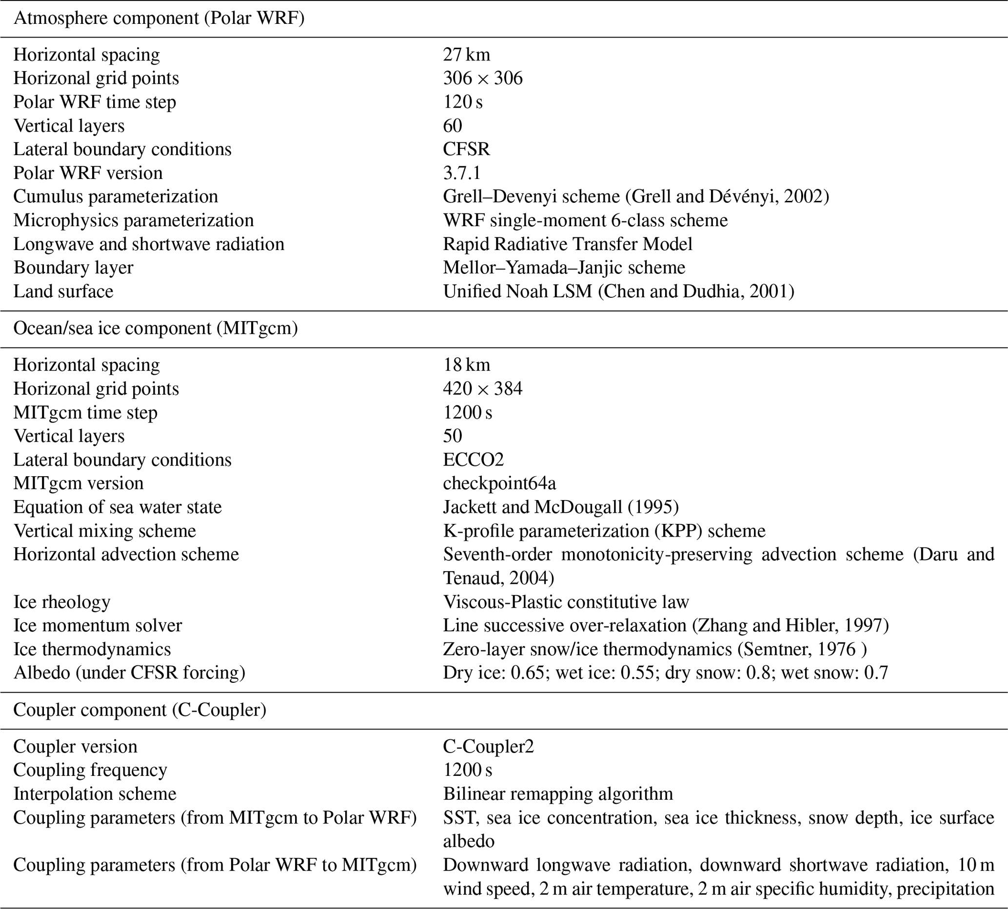
2.1 The oceanic and sea ice component model
The ocean and sea ice component of ArcIOAM is an Arctic configuration of the MITgcm (Nguyen et al., 2011; Liang and Losch, 2018; Liang et al., 2019, 2020). The model has an average horizontal resolution of 18 km and covers the whole Arctic Ocean with open boundaries close to 55∘ N in both the Atlantic and Pacific sectors (Losch et al., 2010). The ocean model includes 420×384 horizontal grid points and 50 vertical model layers based on Arakawa C grid and Z coordinates and a time step of 1200 s. The ocean model uses curvilinear coordinates, and the model grid is locally orthogonal. Vertical resolution of the ocean model layers increases from 10 m near the surface to 456 m near the bottom. The K-profile parameterization (KPP) (Large et al., 1994) is used as the vertical mixing scheme.
The sea ice model shares the same horizontal grid with the ocean model and divides each model grid into two parts: ice and open ocean. In the open-ocean area, ocean–atmosphere heat and momentum fluxes are calculated following the standard bulk formula (Doney et al., 1998). In the ice-covered area, the ice surface and bottom heat and momentum fluxes are calculated according to viscous-plastic dynamics and zero-layer thermodynamics (Hibler, 1980; Semtner, 1976). The so-called zero-layer thermodynamic model assumes one layer of ice underneath one layer of snow and assumes ice does not store heat and therefore tends to exaggerate the seasonal variability in ice thickness. Snow modifies ice surface albedo and conductivity. If enough snow accumulates on top of the ice, its weight submerges the ice and the snow is flooded. In order to parameterize a sub-grid-scale distribution for sea ice thickness, the mean sea ice thickness in each grid can be split into as many as seven thickness categories in the MITgcm sea ice model. In our coupled model for simplicity, we use two thickness categories: open water and sea ice.
2.2 The atmospheric component model
The atmospheric component of ArcIOAM is based on the Polar WRF (Bromwich et al., 2013; Hines and Bromwich, 2008) model, which is an optimized version of the WRF model (Skamarock et al., 2008) for use in polar regions. Previous researchers have made several specific modifications for polar environments, which primarily encompass the land surface model and sea ice to adapt to the particular conditions in Arctic regions. The Noah land surface model is embedded inside the Polar WRF. The changes made in the Noah land surface model (LSM; Chen and Dudhia, 2001) include using the latent heat of sublimation for calculating latent heat flux over ice surface, increasing the snow albedo and the emissivity value for snow, adjusting snow density, modifying thermal diffusivity and snow heat capacity for the subsurface layer, changing the calculation of skin temperature, and assuming ice saturation in calculating the surface saturation mixing ratio over ice. Other modifications of the Polar WRF include a fix to allow specified sea ice quantities and the land mask associated with sea ice to update during a simulation. These modifications improve model performance over the pan-Arctic for short-term forecasts.
The Arctic configuration of the Polar WRF model has been tested and evaluated by a set of simulations over several key surface categories, including large permanent ice sheets with the Greenland/North Atlantic grid and Arctic land (Hines et al., 2011; Hines and Bromwich, 2008) and the production of the Arctic System Reanalysis (ASR) (Bromwich et al., 2010). In this study, the Polar WRF model covers the Arctic regions with a horizontal resolution of 27 km. The model has 306×306 horizontal grid points and 60 vertical layers and a time step of 120 s. The Polar WRF model employed physics options that included the Mellor–Yamada–Janjic boundary layer scheme in conjunction with the Janjic Eta Monin–Obukhov surface layer scheme (Janjić, 2002), the WRF single-moment 6-class microphysics scheme for microphysics, the Grell–Devenyi scheme for clouds (Grell and Dévényi, 2002), and the new version of the rapid radiative transfer model for both shortwave and longwave radiation.
2.3 The coupler
We have implemented the C-Coupler2 to couple the MITgcm and the Polar WRF model. The first version (C-Coupler1) includes features such as a flexible coupling configuration and 3-D coupling capability (Liu et al., 2014). Two coupled models have been built using the C-Coupler1. The first is a coupled climate system model version FGOALS-gc at the Institute of Atmospheric Physics, Chinese Academy of Sciences. The FGOALS-gc can achieve exactly the same (bitwise identical) simulation results as the same model components with a different coupler, the CPL6 (Liu et al., 2014). The second is a regional coupled model FIO-AOW (Zhao et al., 2017) which includes an atmosphere model WRF, an ocean model POM (Princeton Ocean Model) and a wave model MASNUM (Yang et al., 2005).
The second version of the C-Coupler family, the C-Coupler2 (Liu et al., 2018), is equipped with many advanced functions, including (1) a common, flexible, user-friendly coupling configuration interface; (2) the capability of coupling within one executable or the same subset of Message Passing Interface (MPI) processes; (3) flexible and automatic coupling procedure generation for any subset of component models; (4) dynamic 3-D coupling that enables convenient coupling of the field on 3-D grids with time-evolving vertical coordinate values; (5) non-blocking data transfer; (6) model nesting; (7) increment coupling; and (8) adaptive restart capability (Liu et al., 2018).
2.4 Coupling strategy
In ArcIOAM, the requested CPUs are assigned equally to the MITgcm and Polar WRF models. The C-Coupler2 is employed as a library to achieve the two-way parallel coupling between the Polar WRF and the MITgcm (Fig. 1). The coupling interval is set to 20 min. The component models are running in concurrent mode (Fig. 2); that is, the component models run on mutually exclusive sets of cores. If one component model finishes earlier than the other, its resources are idle and wait for the other component model. At each coupling time step, data transfer from the MITgcm to the Polar WRF is executed when data transfer from the Polar WRF to the MITgcm is completed, and vice versa. During coupling execution, the MITgcm sends sea surface temperature (SST), sea ice concentration, sea ice thickness, snow depth and ice surface albedo to the coupler, and these coupling variables are used directly as the bottom boundary conditions in the Polar WRF model. The Polar WRF model sends the atmospheric bottom boundary variables to the coupler, including downward longwave radiation, downward shortwave radiation, 10 m wind speed, 2 m air temperature, 2 m air specific humidity and precipitation. The MITgcm uses these atmospheric variables to compute the open-ocean and ice surface heat, freshwater, and momentum forcing.
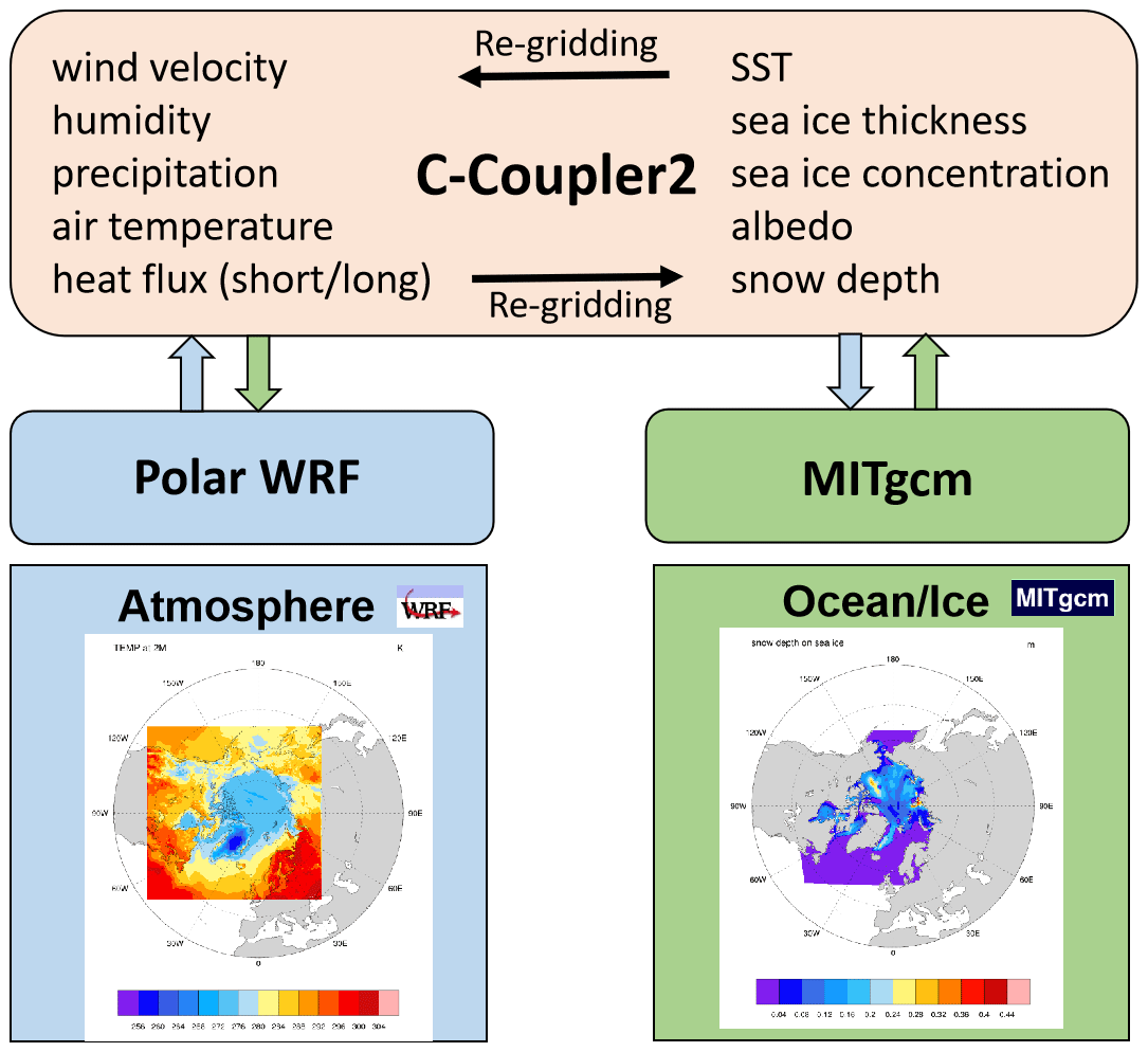
Figure 1Coupling strategy of the Polar WRF-MITgcm coupled model system.
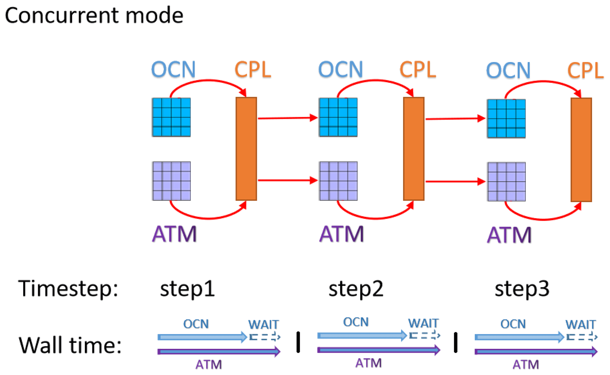
Figure 2Concurrent mode of the coupled model. The small blocks under OCN or above ATM are the small subdomains in each node; the block under CPL is the coupler. The red curve arrows indicate that the component models are sending data to the coupler and the red straight arrows indicate that the component models are reading data from the coupler. The horizontal arrows in the wall time indicate the time axis of each component model and the ticks on the time axis indicate the coupling time steps.
Model domains of the MITgcm and the Polar WRF model are shown in Fig. 3a. As the model domain and grid of the Polar WRF and the MITgcm are generally different, several important procedures are carried out in our coupled system. The model domain of the Polar WRF is larger than that of the MITgcm, producing a non-overlapped area between the MITgcm domain and the Polar WRF domain. Also, the MITgcm model only produces surface variables over ocean, and the Polar WRF model also needs bottom boundary conditions over land. Thus, the coupling variables received by the Polar WRF model need to be concatenated by value in the non-overlapped area and in the land area from an external forcing file, and by value in the overlapped ocean area from the MITgcm model together. To diminish the abrupt value changes from two sources, a simple linear relax zone is designed near the open boundaries of the MITgcm model in both the Atlantic and Pacific sectors (Fig. 3b). The coupling variables (VARrecbyWRF) received by the Polar WRF model can be expressed as follows:
where α is relaxation coefficient, which is equal to 0 in the overlapped ocean area away from the MITgcm open boundaries, and equal to 1 in the land area and in the non-overlapped area away from the MITgcm open boundaries. While in the relax zone, α increases from 0 to 1 linearly from the overlapped side to the non-overlapped side. VARsedbyMIT are the coupling variables which are sent by the MITgcm model. VARextern are the bottom boundary variables of the Polar WRF model which are read from the external forcing file.

Figure 3(a) Model domain of the MITgcm and the Polar WRF model. The red and black lines denote the boundaries of the Polar WRF and the MITgcm model, respectively. (b) Relaxation coefficient for the external forcing file of the Polar WRF bottom boundary conditions.
Normally in coupled models the coupler controls the exchange of heat and momentum fluxes among component models. In our model configuration, instead of coupling fluxes directly, we use the C-Coupler2 to control the exchange of fields between the Polar WRF and the MITgcm. Heat and momentum fluxes are calculated separately in each component model. Both the Polar WRF and the MITgcm use the same bulk formula and similar parameters in calculating fluxes, which guarantees the quasi-conservation of heat and momentum transmission between the component models. The bilinear interpolation algorithm is used to transform model variables between the horizontal grid of the Polar WRF and that of the MITgcm. Figure 4 shows wind stress curl derived from the Polar WRF output and the MITgcm output, as well as their difference on 1 March 2012. It can be seen that the Polar WRF and MITgcm models generate similar wind stress curl pattern, and the difference due to the interpolation algorithm and momentum calculation accounts for less than 5 % of the wind stress curl (Fig. 4c).
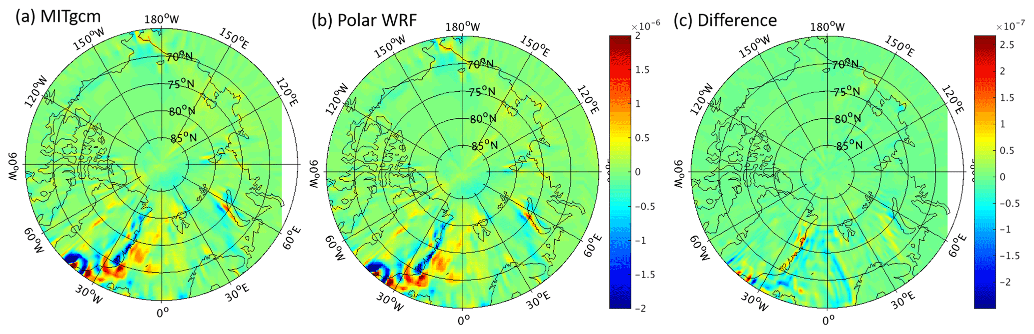
Figure 4Wind stress curl (unit: Nm−2) derived from (a) the MITgcm output, (b) the Polar WRF output and (c) their difference on 1 March 2012. The difference of wind stress curl between the Polar WRF and MITgcm is calculated by interpolating the Polar WRF output onto the MITgcm grid.
In this section, the parallel efficiency of the ArcIOAM is investigated. Different numbers of CPU cores are used to evaluate the parallel speed-up of the coupled model. The CPU elapsed time spent on the coupling interface of each component model in the coupled runs are detailed. Additionally, the parallel efficiency of each component model in the stand-alone runs are calculated for references. The parallel efficiency tests are performed on the high-performance computing cluster at NMEFC. The high-performance computing cluster is a Lenovo Blade Server system composed of 240 dual-socket compute nodes based on 14-core Intel Haswell processors running at 2.4 GHz. Each node has 128 GB DDR4 memory running at 2133 MHz. Overall the system has a total of 6270 CPU cores (240 nodes CPU cores) and has a theoretical peak speed of 258 teraflops. The parallel efficiency of the scalability test is , where Np0 and Npn are the number of CPUs employed in the base case and the test case, respectively; tp0 andtpn represent the CPU elapsed time in the base case and the test case. The speed-up is defined as , which is the relative improvement of the CPU time. The scalability tests are performed by integrating 7 model days for the stand-alone Polar WRF, the stand-alone MITgcm and the coupled runs.
In the ArcIOAM runs, the requested CPUs are assigned equally to the component models. The minimum number of CPUs we use is 28, i. e. Np0 =28. Limited by computational resources, the maximum number of CPUs we can use is 896. The total CPU elapsed time in the coupled runs decreases from 12 840 to 1380 s when the requested CPUs increase from 28 to 896 (Table 2). When the requested CPUs are less than 448, the CPU elapsed time used for numerical integration by the MITgcm is substantially smaller than that for numerical integration by the WRF, meaning that the efficiency of the coupled model depends on the WRF component model. When the requested CPUs are larger than 448, the efficiency of the coupled model depends on the MITgcm component model.
Table 2Comparison of CPU time spent on coupled and stand-alone runs. The CPU time spent on two stand-alone simulations are presented to show the difference between coupled and stand-alone simulations. “total_cpu_number” denotes the requested CPUs, and “total_run_time” denotes the total CPU elapsed time. “wrf_interface”, “wrf_integration”, “mitgcm_interface” and “mitgcm_integration” denote the CPU elapsed time used for coupling interface by the WRF, numerical integration by the WRF, coupling interface by the MITgcm and numerical integration by the MITgcm, respectively. “wrf_time_ alone” denotes the CPU elapsed time of the stand-alone WRF runs. “mitgcm_time_alone” denotes the CPU elapsed time of the stand-alone MITgcm runs. Each run is integrated for 7 model days.
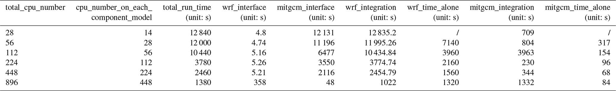
The parallel efficiency of the coupled model remains higher than 90 % when employing less than 112 cores and is still as high as 80 % when using 224 cores (Fig. 5). The parallel efficiency of the stand-alone MITgcm is near to that of the stand-alone Polar WRF when the requested CPUs are less than 448, while both of them are substantially lower than the coupled model. The parallel speed-up of the coupled model is higher than the stand-alone component model. The decrease in parallel efficiency results from the increase in communication time, load imbalance and I/O (read and write) operation per CPU core (Christidis, 2015).
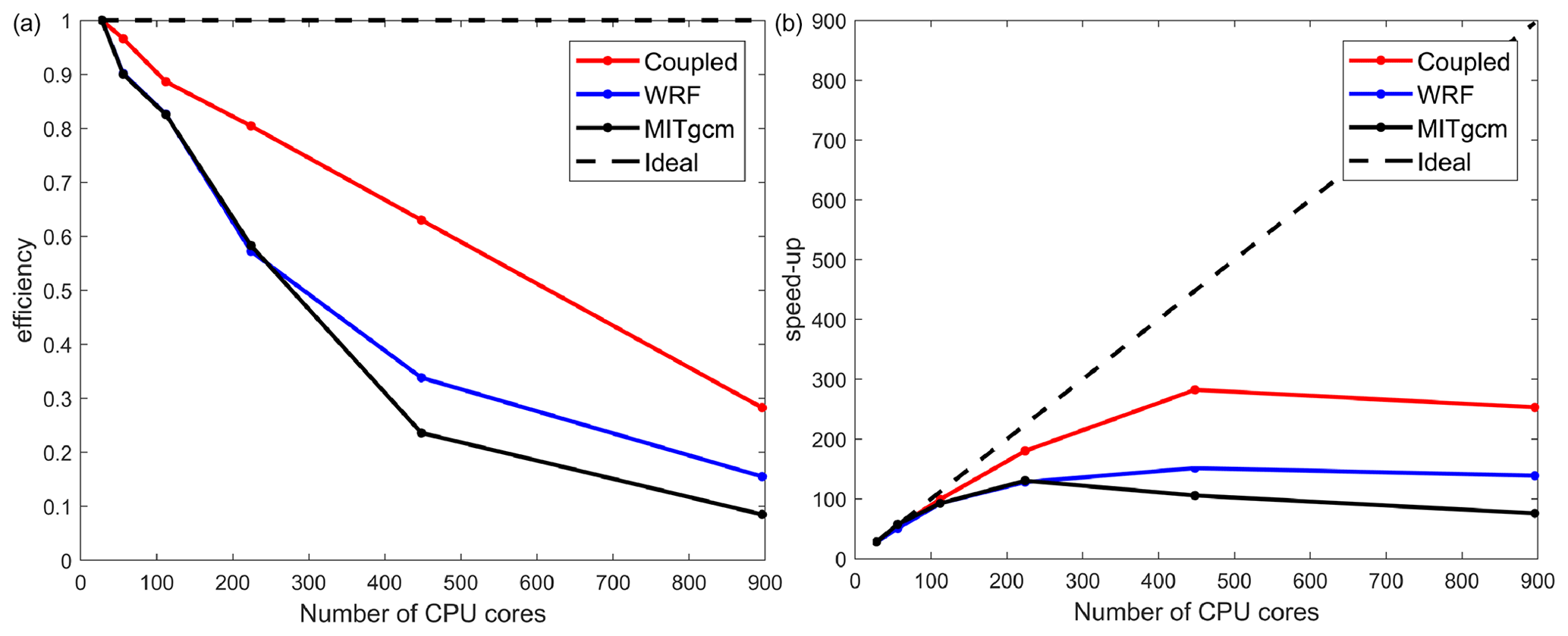
Figure 5The parallel efficiency (a) and speed-up (b) test of the coupled model and the stand-alone component models, employing up to 896 CPU cores. The simulation using 28 CPU cores is regarded as the baseline case when computing the speed-up. The tests are performed on a Lenovo Blade Server system composed of 240 dual-socket compute nodes based on 14-core Intel Haswell processors.

Figure 6Time series of (a) sea ice extent, (b) sea ice extent anomaly and (c) root mean square error (RMSE) of modeled sea ice concentration with respect to the OSISAF observation in 2012. The black, red, green and blue lines in (a) denote sea ice extent of the MASIE observation, the OCNCPL run, the OCNSTA run and the OCNDYN run, respectively. The black, red, green and blue lines in (b) denote sea ice extent anomaly of the MASIE observation, the OCNCPL run, the OCNSTA run and the OCNDYN run, respectively. The red, green and blue lines in (c) denote the sea ice concentration RMSE of the OCNCPL run, the OCNSTA run and the OCNDYN run, respectively. MASIE: Multisensor Analyzed Sea Ice Extent; OSISAF: Ocean and Sea Ice Satellite Application Facility.
As a starting point, we evaluate the performance of ArcIOAM on a seasonal timescale. In this work, we perform the coupled model simulations in the year 2012, because an unusually strong storm formed off the coast of Alaska on 5 August 2012 and tracked into the center of the Arctic Basin, where it lingered for several days and generated strong sea-ice–ocean–atmosphere interaction (Simmonds and Rudeva, 2012). With more open-ocean area exposed to atmosphere, we expect that sea-ice–ocean–atmosphere interaction processes are more intense in the summertime than in the wintertime. In the Arctic regions, there is also higher demand for seasonal prediction in the summertime when more commercial and Arctic shipping occurs. The main aim of this paper is to assess the sea ice and ocean simulation capabilities of the coupled system. For this reason, less attention will be paid to the atmosphere simulation. Future work will emphasize atmospheric variables and seasonal sea ice prediction skill with available observations assimilated.
Three experiments using different coupling strategies are performed in this study (Table 3). The first experiment, which is denoted by OCNCPL, is a two-way coupled simulation where the MITgcm receives the coupled variables from the Polar WRF, and the Polar WRF receives the coupled variables from the MITgcm. The second experiment, which is denoted by OCNDYN, is a one-way coupled simulation where the MITgcm only receives the coupled variables from Polar WRF, but without sending the coupled variables back to Polar WRF. α in Eq. (1) is set to 1 in the OCNDYN run. The third experiment, OCNSTA, represents the stand-alone MITgcm simulation with the same sea ice albedo parameters as the coupled model but prescribed atmospheric forcing to keep consistency with the previous two coupling experiments. The model state deviation between these cases represents the influences of sea-ice–ocean–atmosphere interaction in the Arctic Ocean.
Table 3The initial conditions, boundary conditions and forcing terms used in the experiments.

Atmospheric initial and boundary conditions: CFSR. Oceanic boundary conditions: ECCO2.r Oceanic initial conditions: restart field on 1 January 2012 derived from a stand-alone MITgcm simulation initialized from climatological temperature and salinity field derived from WOA05 and forced by the 3-hourly JRA55 data from 1979 to 2011.
The atmospheric initial and lateral boundary conditions, the bottom boundary conditions in the external forcing file used in the OCNCPL and OCNDYN runs, and the prescribed atmospheric forcing used in the OCNSTA run are derived from the 6-hourly National Centers for Environmental Prediction (NCEP) Climate Forecast System Reanalysis (CFSR) data (Saha et al., 2010). The oceanic monthly lateral boundary condition of the coupled model is derived from the Estimating the Circulation and Climate of the Ocean Phase II (ECCO2) high-resolution global-ocean and sea ice data synthesis (Menemenlis et al., 2008), including potential temperature, salinity, current and sea surface elevation. The discrepancy of atmosphere and ocean boundary condition is less of an issue since the ocean does not vary much on shorter timescales and the zones of sea ice are far away from the lateral boundary. The initial conditions of ocean and sea ice on 1 January 2012 are derived from a stand-alone MITgcm simulation initialized from a climatological temperature and salinity field derived from the World Ocean Atlas 2005 (WOA05) (Locarnini et al., 2006; Antonov et al., 2006) and forced by the 3-hourly Japanese 55-year Reanalysis (JRA55) (Harada et al., 2016; Kobayashi et al., 2015) data from 1979 to 2011 (Liang and Losch, 2018). After a 33-year integration, the ocean and sea ice initial conditions on 1 January 2012 used in the coupled model are retrieved from a quasi-equilibrium ocean–sea-ice evolution period. River runoff is based on the Arctic Runoff Database (Nguyen et al., 2011). The model states are output on a daily basis.
5.1 Sea ice extent and concentration
The minimum Arctic sea ice extent in the satellite era occurred in the summer of 2012 (Francis, 2013). Arctic sea ice extent grew to maximum value of 14.5 million km2 in March 2012 and dropped to minimum value of 3.5 million km2 in September 2012 (Fig. 6a) according to the Multisensor Analyzed Sea Ice Extent – North Hemisphere (MASIE-NH) data (U.S. National Ice Center and National Snow and Ice Data Center, 2010). The MASIE-NH data are provided daily by the National Ice Center Interactive Multisensor Snow and Ice Mapping System with a spatial resolution of 4 km. Compared with the OCNSTA run, results from the experiments with coupling (OCNCPL and OCNDYN) are closer to observations (Fig. 6). It is noted that both the OCNCPL and OCNDYN runs simulate lower sea ice extent than the observations by a bias of 1–1.5 million km2 (Fig. 6a) after the first 2 weeks of January. Because the sea ice initial condition on 1 January 2012 is derived from a stand-alone MITgcm simulation which is forced by the JRA55 data, the change of atmospheric forcing data from the JRA55 to the NCEP CFSR induces a model state adjustment period which lasts about 2 weeks. By comparing the sea ice extent evolution of the OCNCPL and OCNDYN runs, it appears that sea-ice–ocean–atmosphere interaction generates only a small change in sea ice extent. Based on our analysis of the sea ice spatial distribution, sea-ice–ocean–atmosphere interaction plays a decisive role in summertime sea ice spatial distribution.
Figure 6b shows the modeled and observed sea ice extent anomaly. After the model state adjustment period, both the amplitudes and phase of sea ice extent seasonal cycle in the OCNCPL and OCNDYN runs are close to the observations. Results of the stand-alone run show that sea ice melts and freezes in advance of the observations. Nguyen et al. (2011) pointed out that optimized parameters of sea ice and snow albedo depend on selected atmospheric forcing in the MITgcm. In the sea ice model of MITgcm, the actual surface albedo changes with time and is a function of four foundational albedo parameters (dry ice, dry snow, wet ice, wet snow), as well as ice surface temperature and snow depth. A series of sensitivity experiments are performed to get an optimal combination of sea ice parameters (figures not shown). The sea ice model systematic bias could also be reduced by assimilating sea ice data (Liang et al., 2019) when conducting a seasonal sea ice prediction system.
The modeled sea ice concentration is compared with the observations derived from the EUMETSAT Ocean and Sea Ice Satellite Application Facility (OSISAF) (Eastwood et al., 2011). The observations are reprocessed daily sea ice concentration fields which are retrieved from the Scanning Multichannel Microwave Radiometer/Special Sensor Microwave Imager (SMMR/SSMI) data with a spatial resolution of 10 km. Figure 6c shows the root mean square error (RMSE) evolution of the modeled sea ice concentration with respect to the OSISAF data. After 1 month of model state adjustment, three experiments show a similar pattern of RMSE being lower in winter and spring than in summer and autumn. The Arctic basin is almost fully covered by sea ice from November to May (Fig. 7); thus the two coupling experiments do not produce substantial sea ice concentration differences. With more open ocean exposed to atmosphere, from June to September the sea ice concentration RMSE of the OCNCPL run is significantly lower than that of the OCNDYN run. This result indicates that sea-ice–ocean–atmosphere interaction plays a crucial role in controlling Arctic summertime sea ice distribution.
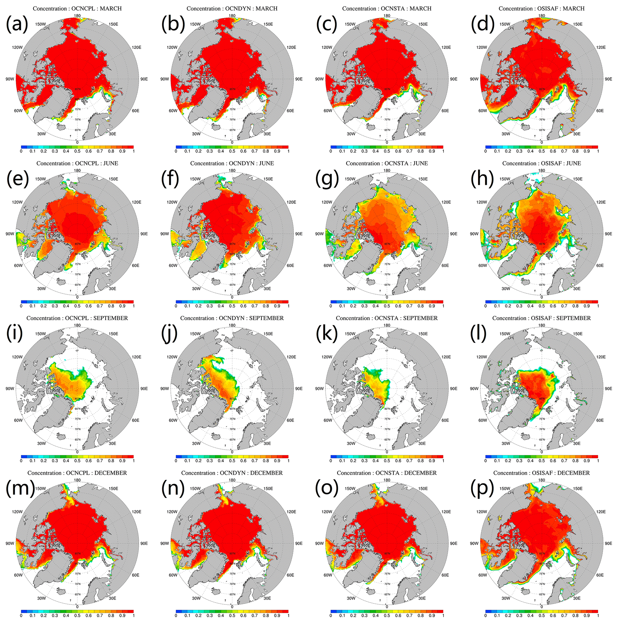
Figure 7Modeled and observed monthly mean sea ice concentration. From top to bottom panels show the March, June, September and December sea ice concentration, respectively. From left to right panels show sea ice concentration of the OCNCPL run, the OCNDYN run, the OCNSTA run and the OSISAF observations. OSISAF: Ocean and Sea Ice Satellite Application Facility.
We show the modeled and observed monthly mean sea ice concentration (Fig. 7) and deviation of model results and observation (Fig. 8) in March, June, September and December. In March, when the Arctic Ocean is almost fully covered by sea ice, the main source of discrepancy appears in sea ice edge zones on the Atlantic side (Fig. 7a–c). In June, sea ice concentrations are overestimated in the Arctic marginal seas in the OCNCPL and OCNDYN runs (Fig. 8d–e). The modeled sea ice concentration in the OCNSTA run is closer to the observations (Fig. 7f) than the two coupled runs. In September, the modeled sea ice in the marginal sea ice zone melts out in all runs (Fig. 7i–k). Compared with the satellite observations (Fig. 7l), sea ice in the OCNSTA run melts over in summertime, which leads to an anomalous negative bias of sea ice concentration in the Arctic (Fig. 8i), and the two coupled runs overestimate sea ice concentration in the southern Beaufort Sea while underestimating sea ice concentration in the center Arctic basin (Fig. 8g–h). Although the two coupled runs simulate similar sea ice extent patterns, due to the inclusion of sea-ice–ocean–atmosphere interaction in the OCNCPL run, the modeled sea ice distribution of the OCNCPL run is closer to the observations (Fig. 7i and l). In December, the situation is similar to that in March when sea ice dominates almost the entire Arctic.

Figure 8Deviation between the modeled and observed monthly mean sea ice concentration. From top to bottom panels show the March, June, September and December sea ice concentration deviation respect to the OSISAF observations, respectively. The left, middle and right panels show results of the OCNCPL run, the OCNDYN run and the OCNSTA run. OSISAF: Ocean and Sea Ice Satellite Application Facility.
5.2 Sea ice volume and thickness
Satellite sea ice thickness data are not currently available in melt seasons from May to September. We compare the modeled sea ice volume with that from a widely used sea ice volume data source (Fig. 9a), the Pan-Arctic Ice Ocean Modeling and Assimilation System (PIOMAS) developed at the Applied Physics Laboratory of the University of Washington (Zhang and Rothrock, 2003). PIOMAS assimilates sea ice concentration data from the National Snow and Ice Data Center (NSIDC) and SST data from NCEP/NCAR Reanalysis. The OCNSTA run simulates more realistic sea ice growth rates from January to May but systematic negative sea ice volume bias compared with the PIOMAS data. The sea ice volume in the OCNCPL and OCNDYN runs shows better results than that in the OCNSTA run from June to December. However, both the two coupled runs produce less sea ice volume than the PIOMAS data in most of 2012, partly because our model underestimates sea ice extent (Fig. 6a) without assimilating observations. It is notable that the sea ice volume evolution of the OCNCPL run is closer to the PIOMAS data at the end of 2012.
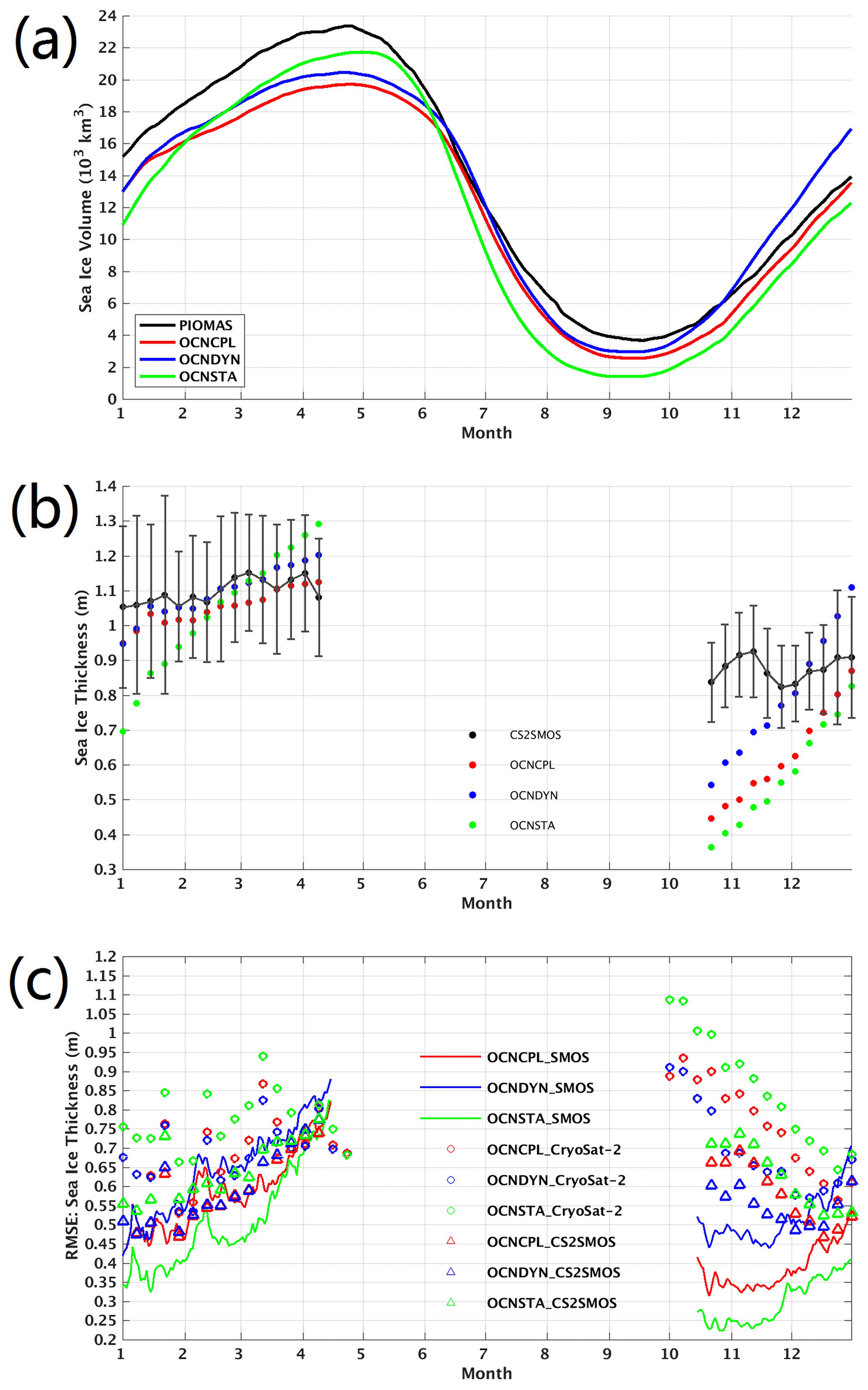
Figure 9Time series of (a) total sea ice volume, (b) spatial mean sea ice thickness and (c) the RMSE of sea ice thickness with respect to the satellite-retrieved observations in 2012. The black, red, green and blue lines in (a) denote total sea ice volume of the PIOMAS data, the OCNCPL run, the OCNSTA run and the OCNDYN run, respectively. The black, red, green and blue dots in (b) denote sea ice thickness of the CS2SMOS observations, the OCNCPL run, the OCNSTA run and the OCNDYN run, respectively. The black bar in (b) represents the observational uncertainties of the CS2SMOS data. The red, green and blue masks in (c) denote sea ice thickness RMSE of the OCNCPL run, the OCNSTA run and the OCNDYN run with respect to the SMOS observations in a thin ice (< 1 m) region (line), the Cryosat-2 observations (circle) and the CS2SMOS observations (triangle), respectively. Model grid points without available observations are not included in the sea ice thickness RMSE calculation. PIOMAS: Pan-Arctic Ice Ocean Modeling and Assimilation System; SMOS: Soil Moisture Ocean Salinity.
Satellite sea ice thickness observations are usually retrieved from either ice surface brightness temperature or radar altimetric measurement of sea ice freeboard. We use three kinds of satellite sea ice thickness data to validate our model results (Fig. 9b and c). Daily sea ice thickness observations provided by the University of Hamburg are derived from the Soil Moisture Ocean Salinity (SMOS) brightness temperature combined with a sea ice thermodynamic model and a three-layer radiative transfer model (Kaleschke et al., 2012). Weekly sea ice thickness observations provided by the Alfred Wegener Institute at the Helmholtz Centre for Polar and Marine Research are derived from the European Space Agency satellite mission CryoSat-2 radar altimetric data (Ricker et al., 2014). The SMOS observations retrieved from satellite brightness temperature data are more accurate in the marginal sea ice zone where ice thickness is thinner than 1 m (Tian-Kunze et al., 2014), while the CryoSat-2 observations retrieved from radar altimetric data have higher accuracies in the pack sea ice zone than in the marginal sea ice zone (Laxon et al., 2013; Wingham et al., 2006). Taking the spatial complementarity of the SMOS and CryoSat-2 data into consideration, Ricker et al. (2017) introduced a weekly sea ice thickness product covering the entire Arctic, the CS2SMOS sea ice thickness, which is generated by merging the SMOS sea ice thickness with the CryoSat-2 sea ice thickness (Ricker et al., 2017). The CS2SMOS data with observational uncertainty are also added to our comparison.
The weekly CryoSat-2 data include several banded sea ice thickness records which are collected in 1 week when polar orbital satellites pass the Arctic region. The SMOS data used in this study are those in the thin ice (< 1 m) region. Considering spatial coverage of the observations, we compare spatial-mean sea ice thickness evolution with the CS2SMOS data (Fig. 9b). Compared with the CS2SMOS data, both coupled runs produce more realistic sea ice thickness evolution than the stand-alone run from January to April. However, large sea ice thickness errors between the model and the observations exist in October and November. We attribute these large errors to the observational uncertainties induced by radar altimetric measurement errors when sea ice starts to freeze. The modeled sea ice in the OCNCPL run is thinner than that in the OCNDYN run, and the sea ice thickness deviations between the two runs amplify after the summer. Meanwhile, the sea ice volume and thickness of the OCNCPL run are closer to the PIOMAS data and the CS2SMOS observations at the end of 2012. Day et al. (2014) pointed out that sea ice thickness incorporates the long-term memory of melting–freezing processes. Notz and Bitz (2017) indicated that summertime sea ice thickness has an important influence on sea ice state in the following spring through the ice-thickness–ice-growth feedback. A negative anomaly of the sea-ice area in late summer induces larger heat losses in autumn and winter from the ocean to the atmosphere due to enhanced outgoing long-wave radiation and turbulent heat fluxes; this causes thinner snow and ice due to later freeze-up and hence larger heat-conduction fluxes through sea ice, eventually leading to larger ice-growth rates. We speculate that in the OCNCPL run sea-ice–ocean–atmosphere interaction causes a more realistic sea ice thickness distribution in the summer of 2012, which preconditions the sea ice thickness evolution in the following freezing season.
The sea ice thickness RMSEs of the three runs with respect to three kinds of satellite sea ice thickness data are shown in Fig. 9c. Compared with the coupled runs, the sea ice thickness in the OCNSTA run shows larger bias in the pack ice zone and a smaller bias in the marginal ice zone. The sea ice thickness RMSE between the OCNCPL run and the SMOS data is smaller than that between the OCNDYN run and the SMOS data, indicating that sea-ice–ocean–atmosphere interaction substantially improves the sea ice thickness simulation in the marginal sea ice zone in the coupled runs. The sea ice thickness RMSEs between the coupled runs and the CryoSat-2 data are generally larger than those between the coupled runs and the CS2SMOS data, especially in October and November, which is partly due to the large uncertainty of radar altimetric measurement when sea ice starts to freeze, and partly due to the low spatial coverage of the CryoSat-2 data.
Normally, satellite sea ice thickness data have large uncertainties due to limitations of the retrieval algorithm. In situ sea ice thickness observations with higher accuracy can provide a direct reference for the model. To further evaluate the modeled sea ice thickness, we compare the time evolution of modeled and in situ observed sea ice thickness at three locations in the Beaufort Sea in 2012 (Fig. 10). The observations are derived from moored upward-looking sonar (ULS) ice draft data from the Beaufort Gyre Exploration Project (BGEP) (Proshutinsky et al., 2005). The ULS samples the ice draft with a precision of 0.1 m (Melling and Riedel, 1995), and the ice draft can be converted to ice thickness assuming hydrostatic equilibrium (Nguyen et al., 2011). Generally speaking, at all three locations in the Beaufort Sea, when the modeled sea ice is thinner than 1 m, the sea ice thickness evolution improves in the OCNCPL run compared with those in the OCNDYN run. This result further demonstrates that sea-ice–ocean–atmosphere interaction plays an important role in marginal sea ice evolution.
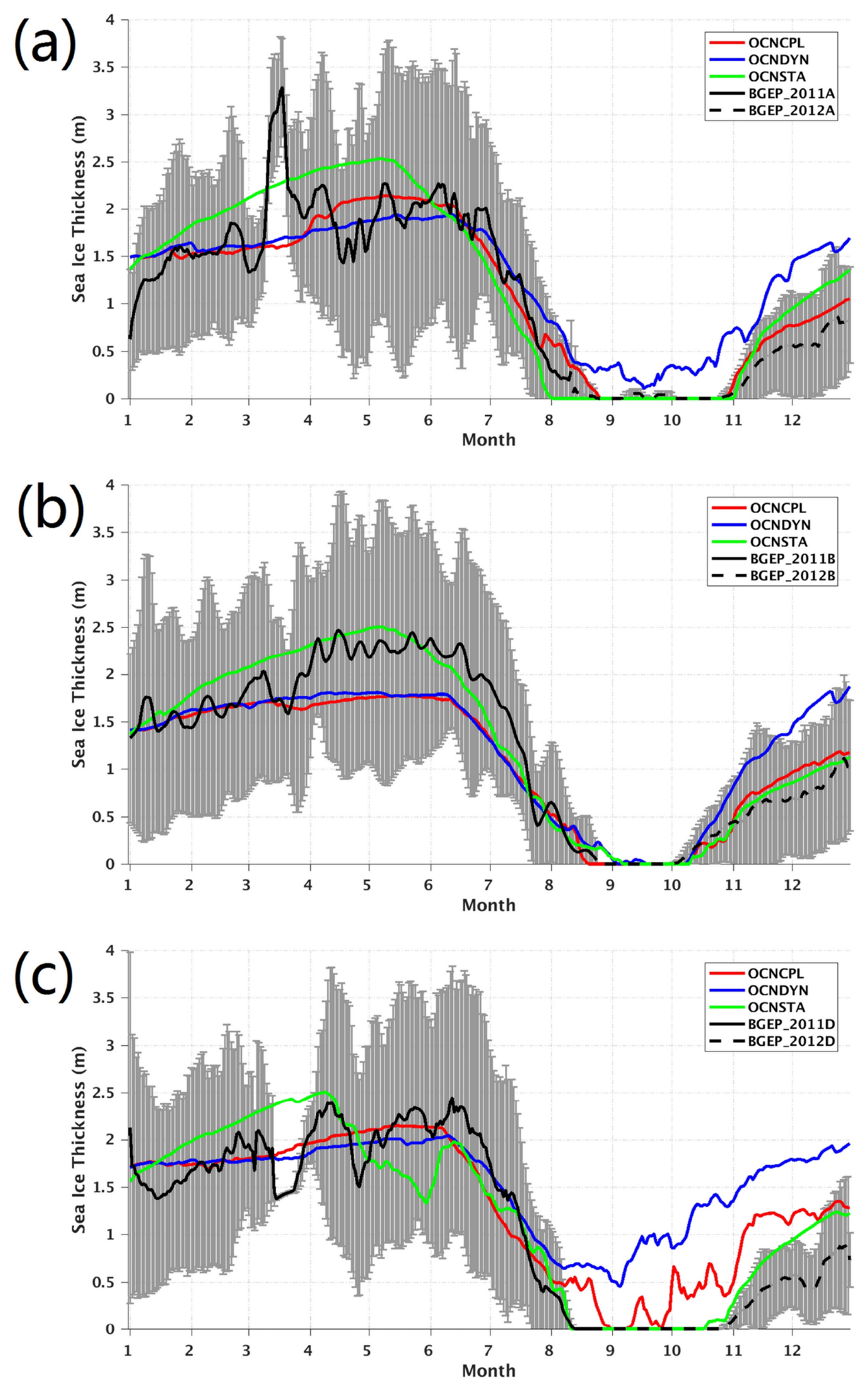
Figure 10Time series of sea ice thickness at three positions: (a) 75∘ N, 150∘ W; (b) 78∘ N, 150∘ W; and (c) 74∘ N, 140∘ W. The red, blue and green lines denote sea ice thickness of the OCNCPL run, the OCNDYN run and the OCNSTA run, respectively. The black solid and dashed lines denote sea ice thickness observations of the BGEP ULSs, which were deployed in the summers of 2011 and 2012. The black lines of the BGEP ULS observations have been smoothed with the gray bar representing the observational uncertainties. BGEP: Beaufort Gyre Exploration Project; ULS: upward-looking sonar.
Spatial distributions of monthly mean sea ice thickness and its bias with respect to available CS2SMOS data in March, June, September and December are shown in Figs. 11 and 12. In March and December, all three runs underestimate sea ice thickness in the central Arctic, while overestimating sea ice thickness in the marginal sea ice zone (Fig. 12). In March, the OCNSTA run overestimates sea ice thickness in the Pacific sector of the Arctic Ocean and in Baffin Bay (Fig. 12e). The coupled runs overestimate sea ice thickness in the northern Barents Sea while underestimating sea ice thickness in the western Chukchi Sea (Fig. 12a and c). In December, compared with the OCNDYN run, the modeled sea ice thickness in marginal sea ice zone in the OCNCPL run is closer to the CS2SMOS data (Fig. 12b), partly due to the more realistic sea ice distribution at the beginning of freezing season, as summertime sea ice thickness has a strong effect on preconditioning the following wintertime sea ice thickness (Day et al., 2014).
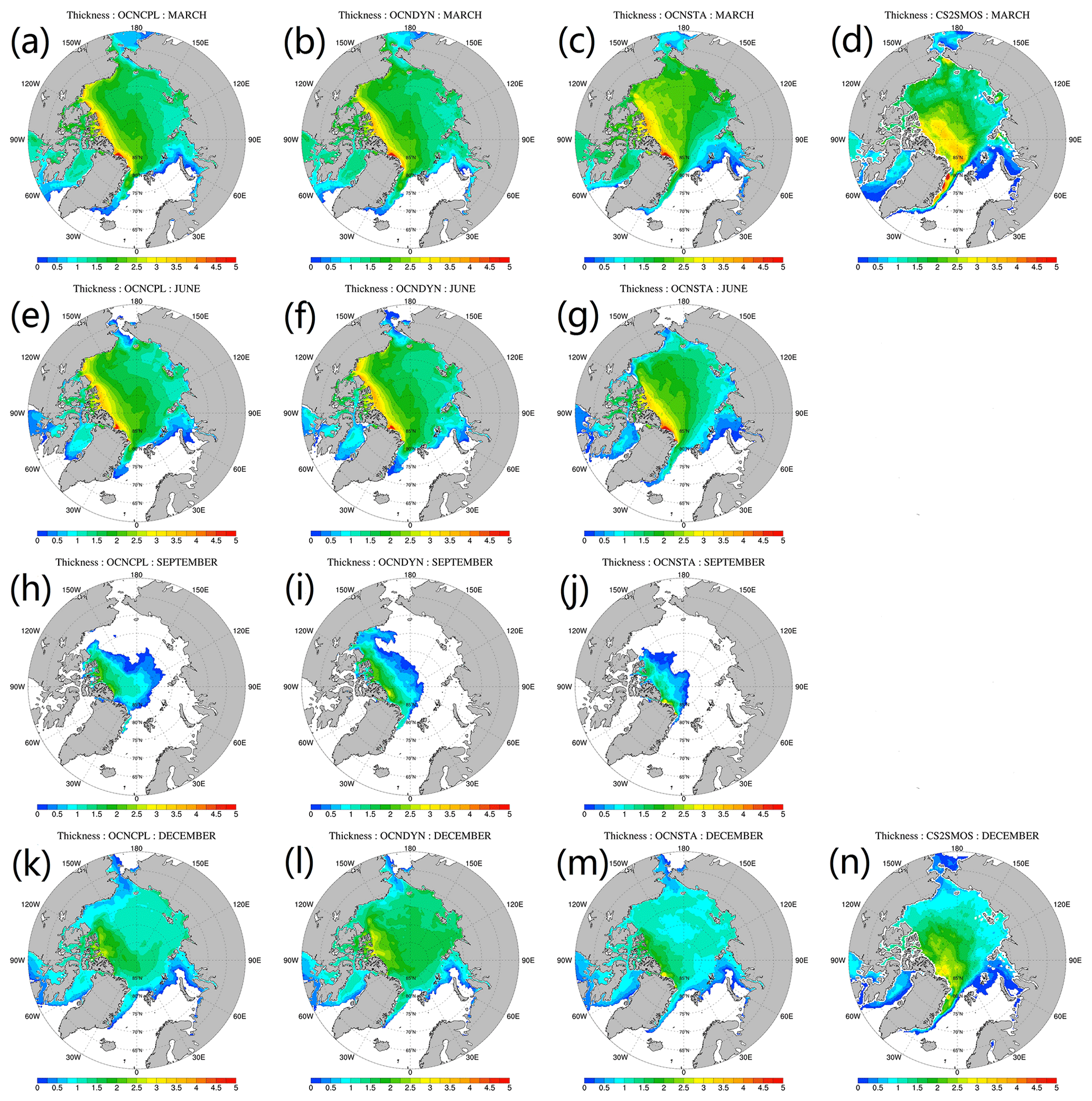
Figure 11Monthly mean sea ice thickness. From top to bottom panels show the March, June, September and December sea ice thickness, respectively. From left to right panels show sea ice thickness of the OCNCPL run, the OCNDYN run, the OCNSTA run and the CS2SMOS data.
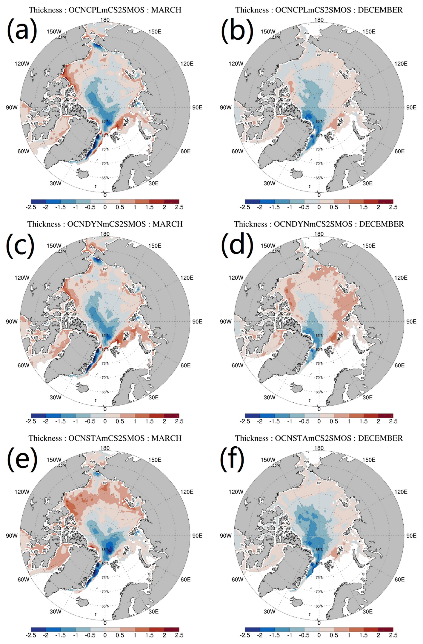
Figure 12Deviation of the modeled monthly mean sea ice thickness and the CS2SMOS data. The top, middle and bottom panels show sea ice thickness deviation of the OCNCPL run, the OCNDYN run and the OCNSTA run, respectively. The left and right panels show results in March and December.
5.3 Ocean temperature and current
Sea ice state is intimately linked to ocean state, both dynamically and thermodynamically. The modeled spatial distribution of sea ice concentration in the OCNCPL run exhibits great improvement compared with the OCNDYN run. Since sea ice in the marginal ice zone is strongly affected by SST through lateral heat transport, we suspect that sea-ice–ocean–atmosphere interaction should impose a positive influence on the modeled ocean temperature in the marginal sea ice zone.
The modeled SST is validated against the Group for High-Resolution SST Multi-Product Ensemble (GMPE) data (Martin et al., 2012). The GMPE SST data provided by the UKMO are a reanalysis daily global SST product that is computed as the median of a large number of SST products. Each product contributing to the GMPE product uses different observational data sets or different retrieval algorithms. As a median product of a multiproduct ensemble, the GMPE SST data greatly reduce observational uncertainties. The SST RMSE of the three runs with respect to the GMPE data are shown in Fig. 13. Compared with the coupled runs, the SST RMSE in the OCNSTA run is smaller in the summertime but larger during the other seasons. Spatial patterns of the modeled and observed SST in March, June, September and December are shown in Fig. 14. Deviation of the modeled SST and the GMPE SST observation is demonstrated in Fig. 15. The GMPE SST data are available in ice-free areas (Fig. 14d, h, l and p). In March and June, the OCNSTA run produces a warmer sea surface in the Nordic Seas, which explains the positive SST bias from January to June in Fig. 13 compared with the coupled runs. In September the SST RMSE in the OCNCPL run (Fig. 13) arises from the strong negative bias in the southern Beaufort Sea and the Baffin Bay (Fig. 15g).
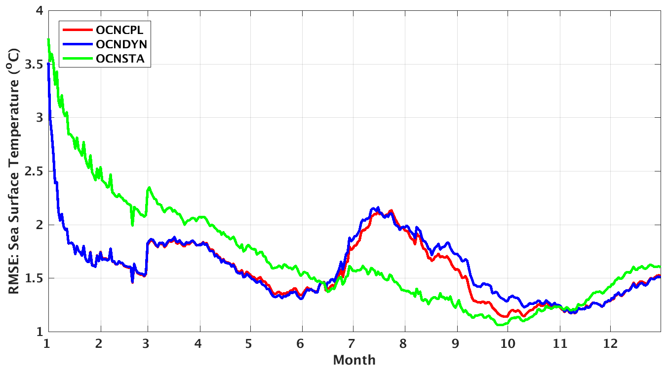
Figure 13Time series of the RMSE of modeled SST with respect to the GMPE observations in 2012. The red, blue and green lines denote the SST RMSE of the OCNCPL run, the OCNDYN run and the OCNSTA run, respectively. GMPE: Group for High-Resolution Sea Surface Temperature Multi-Product Ensemble.

Figure 14Modeled and observed monthly mean SST. From top to bottom panels show the March, June, September and December SST, respectively. From left to right panels show the SST of the OCNCPL run, the OCNDYN run, the OCNSTA run and the GMPE observations, respectively. GMPE: Group for High-Resolution Sea Surface Temperature Multi-Product Ensemble.
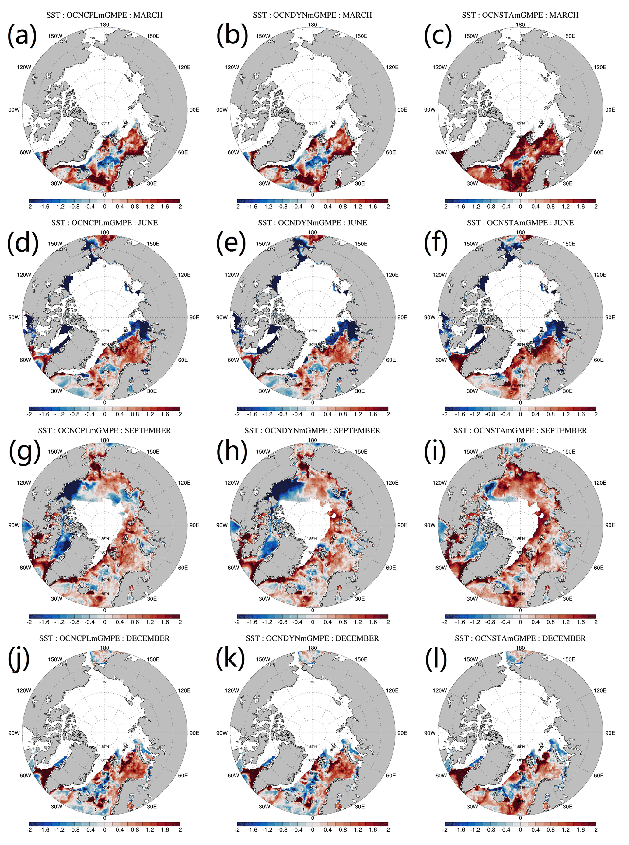
Figure 15Deviation of the modeled monthly mean SST and the GMPE SST data. From top to bottom panels show the March, June, September and December SST deviation, respectively. From left to right panels show the SST of the OCNCPL run, the OCNDYN run and the OCNSTA run, respectively. GMPE: Group for High-Resolution Sea Surface Temperature Multi-Product Ensemble.
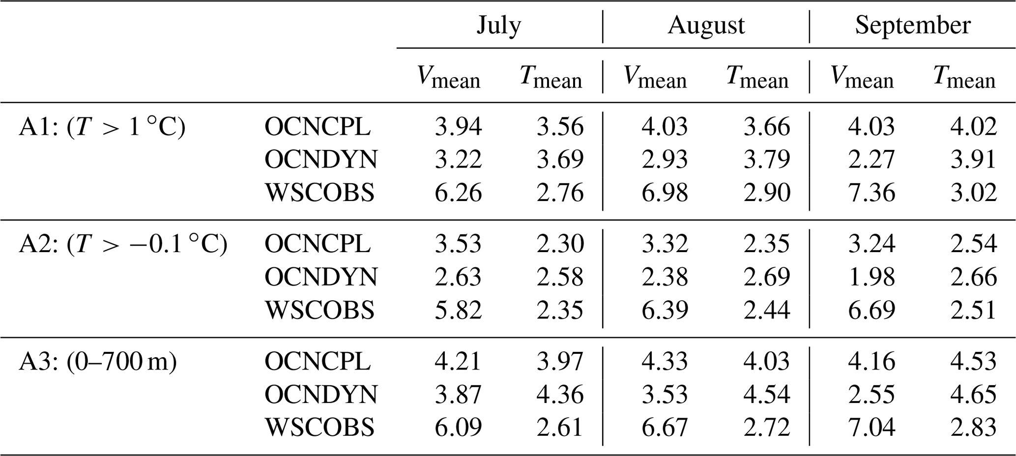
Ocean current observations in the Arctic Ocean are quite sparse, so we evaluate the modeled ocean velocity and temperature with climatological observation generated from the 1998–2003 mooring data in Fram Strait. Under the framework of the European Union projects Variability of Exchanges In the Northern Seas (VEINS) and Arctic Subarctic Ocean Fluxes – North (ASOF-N), a series of moorings in Fram Strait were deployed to record ocean properties since September 1997 to 2004 (Beszczynska, 2011). The observations include the water column from 10 m above the seabed to about 50 m below the surface. Although the observations were conducted at least one decade earlier than 2012, we believe that the comparison between the modeled and observed monthly mean value would likely still apply since the phase of the Atlantic Multidecadal Oscillation did not reverse between 1995 and 2012. The modeled and observed northward cross-section velocity and temperature averaged between 5∘ and E at N are listed in Table 4. The observations show that the northward velocity of the West Spitsbergen Current (WSC) increases from July to September, and the mean temperature of the section of N also increases from July to December. It is notable that the modeled velocity and temperature of the OCNCPL run in Fram Strait are closer to the observations compared with those of the OCNDYN run, although there are still large biases of the modeled velocity between the OCNCPL run and the observations. Vertical temperature distribution in the section averaged between July and September shows that sea-ice–ocean–atmosphere interaction induces warming of the WSC until 700 m depth accompanied with strong cooling beside the WSC (Fig. 16c). The cross-section velocity deviation between the OCNCPL and OCNDYN run is characterized by enhanced northward velocity over the whole water column around 0∘ E and east of 6∘ E, and reduced northward velocity between them (Fig. 16f).

Figure 16July–August–September mean ocean temperature and meridional velocity section along 78∘ N in Fram Strait. The top and bottom panels show the ocean temperature and meridional velocity, respectively. The left, middle and right panels show the OCNCPL run, the OCNDYN run and the deviation between them, respectively.
Table 4Monthly mean northward cross-section velocity (cm/s) and temperature (∘ C) averaged between 5 and E at N in Fram Strait. A1 represents algorithm 1, in which values are calculated from sea water with potential temperature higher than 1 ∘C. A2 represents algorithm 2, in which values are calculated from sea water with potential temperature higher than −0.1 ∘C. A3 represents algorithm 3, in which values are calculated from sea water with depth shallower than 700 m. The observations are averaged between 1998 and 2003. WSCOBS: West Spitsbergen Current Observation.
This paper describes the implementation of an Arctic regional sea-ice–ocean–atmosphere coupled model (ArcIOAM). To connect the component models, a newly developed coupler, C-Coupler2 is implemented to couple the Arctic sea-ice–oceanic configuration of the MITgcm model with the Arctic atmospheric configuration of the Polar WRF model. To couple the Polar WRF and the MITgcm for the first time in the Arctic region, a series of specific procedures including data interpolation between different grids and a relaxation algorithm in lateral boundaries are designed. The parallel efficiency of the coupled model is also investigated.
After implementing ArcIOAM, we demonstrate it with a seasonal simulation of the Arctic sea ice and ocean states in 2012 to evaluate the model capability of seasonal prediction of sea ice. Results from the two-way coupling simulation (OCNCPL), the one-way coupling simulation (OCNDYN) and the stand-alone oceanic simulation (OCNSTA) are compared to a wide variety of available observational and reanalysis products. The model state deviation between the two coupled experiments represents the influences of sea-ice–ocean–atmosphere interaction on the Arctic Ocean and sea ice. From the comparison, results obtained from the two-way coupling experiment best capture the sea ice and ocean evolution in the Arctic region over a 1-year simulation period. The two-way coupling experiment gives better results compared with the one-way coupling experiment and stand-alone oceanic simulation, especially in summertime.
The amplitudes of the sea ice extent seasonal cycle of the two coupled runs are close to the observations. The spatial distribution of sea ice concentration in the OCNCPL run is similar to that in the OCNDYN run from January to May. From June to September the sea ice concentration RMSE of the OCNCPL run with respect to the observations is significantly lower than that of the OCNDYN run, indicating that sea-ice–ocean–atmosphere interaction plays a crucial role in controlling Arctic summertime sea ice distribution. The sea ice thickness RMSE of the OCNCPL run with respect to the SMOS data in thin ice areas is smaller than that of the OCNDYN run. Meanwhile, the evolution of the modeled and observed sea ice thickness at three locations in the Beaufort Sea show that the modeled sea ice thickness evolution improves in the OCNCPL run when the ice is thinner than 1 m. This result means that sea-ice–ocean–atmosphere interaction is very likely to improve the sea ice thickness simulation in the marginal sea ice zone when considering ocean-to-atmosphere feedbacks. Based on comparison with a series of mooring data in Fram Strait, the modeled velocity and temperature in the OCNCPL run are closer to the observations than those in the OCNDYN run, although large biases of the modeled velocity still exist. Compared with the satellite data, the SST obtained in the OCNCPL run is also better than that in the OCNDYN run in summer 2012. The two-way coupling between the Polar WRF and the MITgcm provides a more realistic representation of real air–ice–ocean physical processes, which includes the important ice-albedo feedback in early summer. In the MITgcm, sea ice albedo is calculated based on several variables, such as snow depth on ice and ice surface temperature. In the OCNCPL run, albedo is a coupling variable which affects both the Polar WRF and the MITgcm. In the OCNDYN run, albedo used in the Polar WRF is directly read from the CFSR forcing data. Due to strong sea-ice–ocean–atmosphere interaction in summertime, the two-way coupling strategy not only improves the sea ice simulation, but also benefits the modeled ocean states.
The ArcIOAM is designed for seasonal sea ice prediction up to 6 months, while on longer timescales the regional model's capacity is expected to severely depend on the lateral boundary forcing data. Global coupled models, such as those involved in CMIP6, have innate advantages in sea ice prediction and outlook on seasonal to longer timescales because interactions between high- and mid- latitudes are considered. The land component is also important to the Arctic simulation; however, at the current stage, our coupled model does not have the capacity of coupling an individual land model. Instead we use the embedded land component in the Polar WRF for technical simplicity. It should be noted that the simulation presented in this paper only covers 1 year, and longer simulation results should be carried out to further assess the coupled model. However, given the encouraging results in 2012, this new developed Arctic regional coupled model displays a potential capacity for seasonal sea ice prediction and provides a reliable basis for investigating both thermodynamic and dynamic process and forecasting applications. Meanwhile, bias in the modeled sea ice extent and summertime sea ice thickness still exist, although satellite sea thickness data normally have large uncertainty in summertime, which partly contributes to the large sea ice thickness bias in October–November between the model and CS2SMOS data (Fig. 9b). The foundational sea ice albedo parameters in our current model configuration seem to be underestimated, which allows more heat into the ice and causes thinner sea ice thickness, as well as lower sea ice extent. The choice of sea ice albedo parameters also contributes to the large sea ice thickness bias in October–November between the model and CS2SMOS data. Though the albedo formulation in the MITgcm sea ice model is simple and straightforward, the CICE model provides a more sophisticated scheme for sea ice albedo calculation. In developing operational seasonal sea ice prediction capabilities, the model physics and uncertainty in the coupled model can be improved by using advanced techniques, such as sophisticated sea ice albedo formulation, stochastic physics parameterizations and ensemble approaches. The regional coupled forecasting system can also be improved by involving data assimilation capabilities for initializing the forecasts. Future work will involve exploring these and other aspects for a regional coupled modeling system suited for forecasting and better understanding of mechanisms.
The latest version and future updates of the source code, user guide and examples can be downloaded from https://github.com/cdmpbp123/Coupled_Atm_Ice_Oce (last access: 7 April 2020). The current version of this coupled model (ArcIOAM v1.0) used to produce the results in this paper can be accessed via https://doi.org/10.5281/zenodo.3742692 (Ren et al., 2020).
SR and HY worked on the coding tasks for coupling the Polar WRF with the MITgcm using C-Coupler2. SR and XL designed and performed the simulations for the numerical experiments. SR, HY and XM worked on the technical details for debugging the model and wrote the code documentation. XL worked on the MITgcm model setup and performed sea ice analysis and validation. QS worked on the Polar WRF model setup. XL, HY and BL worked on the scalability test. All authors contributed to the writing of the final article.
The authors declare that they have no conflict of interest.
The authors sincerely thank David Bailey and another anonymous reviewer for their constructive comments. The authors thank the University of Hamburg for providing the SMOS sea ice thickness data (http://icdc.cen.uni-hamburg.de/1/daten/cryosphere/l3c-smos-sit.html, last access: 13 December 2018), the Alfred-Wegener-Institut, Helmholtz Zentrum für Polar- und Meeresforschung for providing the CryoSat-2 (http://data.meereisportal.de/data/cryosat2/version2.0/, last access: 13 December 2018), CS2SMOS sea ice thickness data (https://data.meereisportal-.de/data/cs2smos/version1.4/, last access: 13 December 2018) and Fram Strait mooring data (https://www.whoi.edu/page.do?pid=30914, last access: 13 December 2018), the Norwegian Meteorological Institute for the OSISAF sea ice concentration data (http://www.osi-saf.org/?q=content/sea-ice-products, last access: 13 December 2018), the University of Washington for providing the PIOMAS sea ice volume data (http://psc.apl.uw.edu/research/projects/arctic-sea-ice-volume-anomaly/data/, last access: 13 December 2018), the National Snow and Ice Data Center for providing the MASIE-NH data (http://nsidc.org/data/masie/, last access: 13 December 2018), the Woods Hole Oceanographic Institution for providing the BGEP ULS data (http://www.whoi.edu/beaufortgyre, last access: 13 December 2018), and the Copernicus Marine Environment Monitoring Service for providing the GMPE SST data (http://marine.copernicus.eu/, last access: 13 December 2018).
This research has been supported by the National Key R&D Program of China (grant nos. 2016YFC1402700 and 2018YFC1407200) and the National Natural Science Foundation of China (grant no. 41806003).
This paper was edited by Alexander Robel and reviewed by David Bailey and one anonymous referee.
Antonov, J. I., Locarnini, R., Boyer, T., Mishonov, A., Garcia, H., and Levitus, S.: World Ocean Atlas 2005 Volume 2: Salinity, NOAA Atlas NESDIS, 62, 2006.
Bailey, D. A., Holland, M. M., DuVivier, A. K., Hunke, E. C., and Turner, A. K.: Impact of a New Sea Ice Thermodynamic Formulation in the CESM2 Sea Ice Component, J. Adv. Model. Earth Sy., 12, e2020MS002154, https://doi.org/10.1029/2020MS002154, 2020.
Beszczynska, A.: Validation Data – WSC Moorings, available at: https://www.whoi.edu/page.do?pid=30914 (last access: 16 December 2018), 2011.
Brassington, G. B., Martin, M. J., Tolman, H. L., Akella, S., Balmeseda, M., Chambers, C. R. S., Chassignet, E., Cummings, J. A., Drillet, Y., Jansen, P. A. E. M., Laloyaux, P., Lea, D., Mehra, A., Mirouze, I., Ritchie, H., Samson, G., Sandery, P. A., Smith, G. C., Suarez, M., and Todling, R.: Progress and challenges in short- to medium-range coupled prediction, J. Oper. Oceanogr., 8, s239–s258, https://doi.org/10.1080/1755876X.2015.1049875, 2015.
Bromwich, D., Kuo, Y.-H., Serreze, M., Walsh, J., Bai, L.-S., Barlage, M., Hines, K., and Slater, A.: Arctic System Reanalysis: Call for Community Involvement, Eos T. Am. Geophys. Un., 91, 13–14, https://doi.org/10.1029/2010EO020001, 2010.
Bromwich, D. H., Otieno, F. O., Hines, K. M., Manning, K. W., and Shilo, E.: Comprehensive evaluation of polar weather research and forecasting model performance in the Antarctic, J. Geophys. Res.-Atmos., 118, 274–292, https://doi.org/10.1029/2012JD018139, 2013.
Brown, A., Milton, S., Cullen, M., Golding, B., Mitchell, J., and Shelly, A.: Unified Modeling and Prediction of Weather and Climate: A 25-Year Journey, B. Am. Meteorol. Soc., 93, 1865–1877, https://doi.org/10.1175/BAMS-D-12-00018.1, 2012.
Cassano, J. J., DuVivier, A., Roberts, A., Hughes, M., Seefeldt, M., Brunke, M., Craig, A., Fisel, B., Gutowski, W., Hamman, J., Higgins, M., Maslowski, W., Nijssen, B., Osinski, R., and Zeng, X.: Development of the Regional Arctic System Model (RASM): Near-Surface Atmospheric Climate Sensitivity, J. Climate, 30, 5729–5753, https://doi.org/10.1175/jcli-d-15-0775.1, 2017.
Chen, F., and Dudhia, J.: Coupling an Advanced Land Surface–Hydrology Model with the Penn State–NCAR MM5 Modeling System. Part I: Model Implementation and Sensitivity, Mon. Weather Rev., 129, 569–585, https://doi.org/10.1175/1520-0493(2001)129<0569:caalsh>2.0.co; 2, 2001.
Chen, S., Campbell, T. J., Jin, H., Gaberšek, S., Hodur, R. M., and Martin, P.: Effect of Two-Way Air–Sea Coupling in High and Low Wind Speed Regimes, Mon. Weather Rev., 138, 3579–3602, https://doi.org/10.1175/2009mwr3119.1, 2010.
Christidis, Z.: Performance and Scaling of WRF on Three Different Parallel Supercomputers, in: High Performance Computing, 30th International Conference, ISC High Performance 2015, Frankfurt, Germany, 12–16 July 2015, Springer, Cham, 514–528, 2015.
Craig, A., Valcke, S., and Coquart, L.: Development and performance of a new version of the OASIS coupler, OASIS3-MCT_3.0, Geosci. Model Dev., 10, 3297–3308, https://doi.org/10.5194/gmd-10-3297-2017, 2017.
Daru, V. and Tenaud, C.: High order one-step monotonicity-preserving schemes for unsteady compressible flow calculations, J. Comput. Phys., 193, 563–594, 2004.
Day, J. J., Hawkins, E., and Tietsche, S.: Will Arctic sea ice thickness initialization improve seasonal forecast skill?, Geophys. Res. Lett., 41, 7566–7575, https://doi.org/10.1002/2014GL061694, 2014.
DeLuca, C., Theurich, G., and Balaji, V.: The Earth System Modeling Framework, in: Earth System Modelling – Volume 3: Coupling Software and Strategies, edited by: Valcke, S., Redler, R., and Budich, R., Springer, Berlin, Heidelberg, 43–54, 2012.
Doney, S. C., Large, W. G., and Bryan, F. O.: Surface Ocean Fluxes and Water-Mass Transformation Rates in the Coupled NCAR Climate System Model, J. Climate, 11, 1420–1441, https://doi.org/10.1175/1520-0442(1998)011<1420:sofawm>2.0.co; 2, 1998.
Dupont, F., Higginson, S., Bourdallé-Badie, R., Lu, Y., Roy, F., Smith, G. C., Lemieux, J.-F., Garric, G., and Davidson, F.: A high-resolution ocean and sea-ice modelling system for the Arctic and North Atlantic oceans, Geosci. Model Dev., 8, 1577–1594, https://doi.org/10.5194/gmd-8-1577-2015, 2015.
Eastwood, S., Larsen, K. R., Lavergne, T., Nielsen, E., and Tonboe, R.: Global sea ice concentration reprocessing Product User Manual, EUMETSAT OSISAF, 2011.
Faucher, M., Roy, F., Desjardins, S., Fogarty, C., Pellerin, P., Ritchie, H., and Denis, B.: Operational coupled atmosphere – ocean – ice forecast system for the Gulf of St. Lawrence, Canada, 9th EMS Annual Meeting, Toulouse, France, 28 September–2 October 2009, EMS2009-274, available at: https://ui.adsabs.harvard.edu/abs/2009ems..confE.274F/abstract (last access: 10 October 2018), 2009.
Francis, J. A.: The where and when of wetter and drier: disappearing Arctic sea ice plays a role, Environ. Res. Lett., 8, 041002, https://doi.org/10.1088/1748-9326/8/4/041002, 2013.
Grell, G. A. and Dévényi, D.: A generalized approach to parameterizing convection combining ensemble and data assimilation techniques, Geophys. Res. Lett., 29, 38-31–38-34, https://doi.org/10.1029/2002gl015311, 2002.
Harada, Y., Kamahori, H., Kobayashi, C., Endo, H., Kobayashi, S., Ota, Y., Onoda, H., Onogi, K., Miyaoka, K., and Takahashi, K.: The JRA-55 Reanalysis: Representation of Atmospheric Circulation and Climate Variability, J. Meteorol. Soc. Jpn., 94, 269–302, https://doi.org/10.2151/jmsj.2016-015, 2016.
Hibler, W. D.: Modeling a Variable Thickness Sea Ice Cover, Mon. Weather Rev., 108, 1943–1973, https://doi.org/10.1175/1520-0493(1980)108<1943:MAVTSI>2.0.CO; 2, 1980.
Hines, K. M. and Bromwich, D. H.: Development and Testing of Polar Weather Research and Forecasting (WRF) Model. Part I: Greenland Ice Sheet Meteorology, Mon. Weather Rev., 136, 1971–1989, https://doi.org/10.1175/2007mwr2112.1, 2008.
Hines, K. M., Bromwich, D. H., Bai, L.-S., Barlage, M., and Slater, A. G.: Development and Testing of Polar WRF. Part III: Arctic Land, J. Climate, 24, 26–48, https://doi.org/10.1175/2010JCLI3460.1, 2011.
Jackett, D. R. and McDougall, T. J.: Minimal Adjustment of Hydrographic Profiles to Achieve Static Stability, J. Atmos. Ocean. Techn., 12, 381–389, https://doi.org/10.1175/1520-0426(1995)012<0381:MAOHPT>2.0.CO; 2, 1995.
Janjić, Z.: Nonsingular Implementation of the Mellor-Yamada Level 2.5 Scheme in the NCEP Meso model (NCEP Office Note No. 437), NCEP, Camp Springs, Md, 2002.
Jung, T., Gordon, N. D., Bauer, P., Bromwich, D. H., Chevallier, M., Day, J. J., Dawson, J., Doblas-Reyes, F., Fairall, C., Goessling, H. F., Holland, M., Inoue, J., Iversen, T., Klebe, S., Lemke, P., Losch, M., Makshtas, A., Mills, B., Nurmi, P., Perovich, D., Reid, P., Renfrew, I. A., Smith, G., Svensson, G., Tolstykh, M., and Yang, Q.: Advancing Polar Prediction Capabilities on Daily to Seasonal Time Scales, B. Am. Meteorol. Soc., 97, 1631–1647, https://doi.org/10.1175/bams-d-14-00246.1, 2016.
Kaleschke, L., Tian-Kunze, X., Maaß, N., Mäkynen, M., and Drusch, M.: Sea ice thickness retrieval from SMOS brightness temperatures during the Arctic freeze-up period, Geophys. Res. Lett., 39, L05501, https://doi.org/10.1029/2012GL050916, 2012.
Kobayashi, S., Ota, Y., Harada, Y., Ebita, A., Moriya, M., Onoda, H., Onogi, K., Kamahori, H., Kobayashi, C., Endo, H., Miyaoka, K., and Takahashi, K.: The JRA-55 Reanalysis: General Specifications and Basic Characteristics, J. Meteorol. Soc. Jpn., 93, 5–48, https://doi.org/10.2151/jmsj.2015-001, 2015.
Large, W. G., Mcwilliams, J. C., and Doney, S. C.: Oceanic vertical mixing: A review and a model with a nonlocal boundary layer parameterization, Rev. Geophys., 32, 363–403, 1994.
Laxon, S. W., Giles, K. A., Ridout, A. L., Wingham, D. J., Willatt, R., Cullen, R., Kwok, R., Schweiger, A., Zhang, J., Haas, C., Hendricks, S., Krishfield, R., Kurtz, N., Farrell, S., and Davidson, M.: CryoSat-2 estimates of Arctic sea ice thickness and volume, Geophys. Res. Lett., 40, 732–737, https://doi.org/10.1002/grl.50193, 2013.
Liang, X. and Losch, M.: On the Effects of Increased Vertical Mixing on the Arctic Ocean and Sea Ice, J. Geophys. Res.-Oceans, 123, 9266–9282, https://doi.org/10.1029/2018jc014303, 2018.
Liang, X., Losch, M., Nerger, L., Mu, L., Yang, Q., and Liu, C.: Using Sea Surface Temperature Observations to Constrain Upper Ocean Properties in an Arctic Sea Ice-Ocean Data Assimilation System, J. Geophys. Res.-Oceans, 124, 4727–4743, https://doi.org/10.1029/2019jc015073, 2019.
Liang, X., Zhao, F., Li, C., Zhang, L., and Li, B.: Evaluation of ArcIOPS sea ice forecasting products during the ninth CHINARE-Arctic in summer 2018, Adv. Polar Sci., 31, 19–30, 2020.
Liu, L., Yang, G., Wang, B., Zhang, C., Li, R., Zhang, Z., Ji, Y., and Wang, L.: C-Coupler1: a Chinese community coupler for Earth system modeling, Geosci. Model Dev., 7, 2281–2302, https://doi.org/10.5194/gmd-7-2281-2014, 2014.
Liu, L., Zhang, C., Li, R., Wang, B., and Yang, G.: C-Coupler2: a flexible and user-friendly community coupler for model coupling and nesting, Geosci. Model Dev., 11, 3557–3586, https://doi.org/10.5194/gmd-11-3557-2018, 2018.
Locarnini, R. A., Mishonov, A., Antonov, J., Boyer, T., Garcia, H., and Levitus, S.: World Ocean Atlas 2005 Volume 1: Temperature NOAA Atlas NESDIS, 61, 2006.
Losch, M., Menemenlis, D., Campin, J.-M., Heimbach, P., and Hill, C.: On the formulation of sea-ice models. Part 1: Effects of different solver implementations and parameterizations, Ocean Model., 33, 129–144, https://doi.org/10.1016/j.ocemod.2009.12.008, 2010.
Lynch, A. H., Chapman, W. L., Walsh, J. E., and Weller, G.: Development of a Regional Climate Model of the Western Arctic, J. Climate, 8, 1555–1570, https://doi.org/10.1175/1520-0442(1995)008<1555:doarcm>2.0.co;2, 1995.
Marshall, J., Hill, C., Perelman, L., and Adcroft, A.: Hydrostatic, quasi-hydrostatic, and nonhydrostatic ocean modeling, J. Geophys. Res.-Oceans, 102, 5733–5752, https://doi.org/10.1029/96jc02776, 1997.
Martin, M., Dash, P., Ignatov, A., Banzon, V., Beggs, H., Brasnett, B., Cayula, J.-F., Cummings, J., Donlon, C., Gentemann, C., Grumbine, R., Ishizaki, S., Maturi, E., Reynolds, R. W., and Roberts-Jones, J.: Group for High Resolution Sea Surface temperature (GHRSST) analysis fields inter-comparisons. Part 1: A GHRSST multi-product ensemble (GMPE), Deep-Sea Res. Pt. II, 77–80, 21–30, https://doi.org/10.1016/j.dsr2.2012.04.013, 2012.
Maslowski, W., Clement Kinney, J., Higgins, M., and Roberts, A.: The Future of Arctic Sea Ice, Annu. Rev. Earth Pl. Sc., 40, 625–654, https://doi.org/10.1146/annurev-earth-042711-105345, 2012.
Melling, H. and Riedel, D. A.: The underside topography of sea ice over the continental shelf of the Beaufort Sea in the winter of 1990, J. Geophys. Res.-Oceans, 100, 13641–13653, https://doi.org/10.1029/95JC00309, 1995.
Menemenlis, D., Campin, J. M., Heimbach, P., Hill, C., Lee, T., Nguyen, A., Schodlok, M., and Zhang, H.: ECCO2: High resolution global ocean and sea ice data synthesis, Ocean Q. Newsl., 31, 13–21, 2008.
Neelin, J. D., Latif, M., and Jin, F.: Dynamics of Coupled Ocean-Atmosphere Models: The Tropical Problem, Annu. Rev. Fluid Mech., 26, 617–659, https://doi.org/10.1146/annurev.fl.26.010194.003153, 1994.
Nguyen, A. T., Menemenlis, D., and Kwok, R.: Arctic ice-ocean simulation with optimized model parameters: Approach and assessment, J. Geophys. Res.-Oceans, 116, C04025, https://doi.org/10.1029/2010JC006573, 2011.
Notz, D. and Bitz, C. M.: Sea ice in Earth system models, in: Sea Ice, edited by: Thomas, D. N., Wiley, US, 304–325, https://doi.org/10.1002/9781118778371.ch12, 2017.
Pellerin, P., Ritchie, H., Saucier, F. J., Roy, F., Desjardins, S., Valin, M., and Lee, V.: Impact of a Two-Way Coupling between an Atmospheric and an Ocean-Ice Model over the Gulf of St. Lawrence, Mon. Weather Rev., 132, 1379–1398, https://doi.org/10.1175/1520-0493(2004)132<1379:ioatcb>2.0.co;2, 2004.
Posey, P. G., Metzger, E. J., Wallcraft, A. J., Hebert, D. A., Allard, R. A., Smedstad, O. M., Phelps, M. W., Fetterer, F., Stewart, J. S., Meier, W. N., and Helfrich, S. R.: Improving Arctic sea ice edge forecasts by assimilating high horizontal resolution sea ice concentration data into the US Navy's ice forecast systems, The Cryosphere, 9, 1735–1745, https://doi.org/10.5194/tc-9-1735-2015, 2015.
Proshutinsky, A., Yang, J., Krishfield, R., Gerdes, R., Karcher, M., Kauker, F., Koeberle, C., Hakkinen, S., Hibler, W., Holland, D., Maqueda, M., Holloway, G., Hunke, E., Maslowski, W., Steele, M., and Zhang, J.: Arctic ocean study: Synthesis of model results and observations, Eos T. Am. Geophys. Un., 86, 368–371, https://doi.org/10.1029/2005EO400003, 2005.
Ren, S., Yu, H., Liang, X., and Mai, X.: A fully coupled Arctic sea ice-ocean-atmosphere model (ArcIOAM) based on C-Coupler2, (Version 1.0), Zenodo, https://doi.org/10.5281/zenodo.3742692, 2020.
Ricker, R., Hendricks, S., Helm, V., Skourup, H., and Davidson, M.: Sensitivity of CryoSat-2 Arctic sea-ice freeboard and thickness on radar-waveform interpretation, The Cryosphere, 8, 1607–1622, https://doi.org/10.5194/tc-8-1607-2014, 2014.
Ricker, R., Hendricks, S., Kaleschke, L., Tian-Kunze, X., King, J., and Haas, C.: A weekly Arctic sea-ice thickness data record from merged CryoSat-2 and SMOS satellite data, The Cryosphere, 11, 1607–1623, https://doi.org/10.5194/tc-11-1607-2017, 2017.
Rinke, A., Lynch, A. H., and Dethloff, K.: Intercomparison of Arctic regional climate simulations: Case studies of January and June 1990, J. Geophys. Res.-Atmos., 105, 29669–29683, https://doi.org/10.1029/2000jd900325, 2000.
Saha, S., Moorthi, S., Pan, H.-L., Wu, X., Wang, J., Nadiga, S., Tripp, P., Kistler, R., Woollen, J., Behringer, D., Liu, H., Stokes, D., Grumbine, R., Gayno, G., Wang, J., Hou, Y.-T., Chuang, H.-y., Juang, H.-M. H., Sela, J., Iredell, M., Treadon, R., Kleist, D., Delst, P. V., Keyser, D., Derber, J., Ek, M., Meng, J., Wei, H., Yang, R., Lord, S., Dool, H. v. d., Kumar, A., Wang, W., Long, C., Chelliah, M., Xue, Y., Huang, B., Schemm, J.-K., Ebisuzaki, W., Lin, R., Xie, P., Chen, M., Zhou, S., Higgins, W., Zou, C.-Z., Liu, Q., Chen, Y., Han, Y., Cucurull, L., Reynolds, R. W., Rutledge, G., and Goldberg, M.: The NCEP Climate Forecast System Reanalysis, B. Am. Meteorol. Soc., 91, 1015–1058, https://doi.org/10.1175/2010bams3001.1, 2010.
Schrum, C., Hübner, U., Jacob, D., and Podzun, R.: A coupled atmosphere/ice/ocean model for the North Sea and the Baltic Sea, Clim. Dynam., 21, 131–151, https://doi.org/10.1007/s00382-003-0322-8, 2003.
Semtner, A. J.: A Model for the Thermodynamic Growth of Sea Ice in Numerical Investigations of Climate, J. Phys. Oceanogr., 6, 379–389, https://doi.org/10.1175/1520-0485(1976)006<0379:amfttg>2.0.co;2, 1976.
Simmonds, I. and Rudeva, I.: The great Arctic cyclone of August 2012, Geophys. Res. Lett., 39, L23709, https://doi.org/10.1029/2012gl054259, 2012.
Skachko, S., Buehner, M., Laroche, S., Lapalme, E., Smith, G., Roy, F., Surcel-Colan, D., Bélanger, J.-M., and Garand, L.: Weakly coupled atmosphere–ocean data assimilation in the Canadian global prediction system (v1), Geosci. Model Dev., 12, 5097–5112, https://doi.org/10.5194/gmd-12-5097-2019, 2019.
Skamarock, W. C., Klemp, J. B., Dudhia, J., Gill, D. O., Barker, D., and Duda, M. G.: A Description of the Advanced Research WRF Version 3 (No. NCAR/TN-475+STR), University Corporation for Atmospheric Research, https://doi.org/10.5065/D68S4MVH, 2008.
Smith, G. C., Roy, F., Mann, P., Dupont, F., Brasnett, B., Lemieux, J.-F., Laroche, S., and Bélair, S.: A new atmospheric dataset for forcing ice–ocean models: Evaluation of reforecasts using the Canadian global deterministic prediction system, Q. J. Roy. Meteor. Soc., 140, 881–894, https://doi.org/10.1002/qj.2194, 2014.
Smith, G. C., Roy, F., Reszka, M., Surcel Colan, D., He, Z., Deacu, D., Belanger, J.-M., Skachko, S., Liu, Y., Dupont, F., Lemieux, J.-F., Beaudoin, C., Tranchant, B., Drévillon, M., Garric, G., Testut, C.-E., Lellouche, J.-M., Pellerin, P., Ritchie, H., Lu, Y., Davidson, F., Buehner, M., Caya, A., and Lajoie, M.: Sea ice forecast verification in the Canadian Global Ice Ocean Prediction System, Q. J. Roy. Meteor. Soc., 142, 659–671, https://doi.org/10.1002/qj.2555, 2016.
Smith, G. C., Bélanger, J.-M., Roy, F., Pellerin, P., Ritchie, H., Onu, K., Roch, M., Zadra, A., Colan, D. S., Winter, B., Fontecilla, J.-S., and Deacu, D.: Impact of Coupling with an Ice–Ocean Model on Global Medium-Range NWP Forecast Skill, Mon. Weather Rev., 146, 1157–1180, https://doi.org/10.1175/MWR-D-17-0157.1, 2018.
Sun, R., Subramanian, A. C., Miller, A. J., Mazloff, M. R., Hoteit, I., and Cornuelle, B. D.: SKRIPS v1.0: a regional coupled ocean–atmosphere modeling framework (MITgcm–WRF) using ESMF/NUOPC, description and preliminary results for the Red Sea, Geosci. Model Dev., 12, 4221–4244, https://doi.org/10.5194/gmd-12-4221-2019, 2019.
Tian-Kunze, X., Kaleschke, L., Maaß, N., Mäkynen, M., Serra, N., Drusch, M., and Krumpen, T.: SMOS-derived thin sea ice thickness: algorithm baseline, product specifications and initial verification, The Cryosphere, 8, 997–1018, https://doi.org/10.5194/tc-8-997-2014, 2014.
U.S. National Ice Center and National Snow and Ice Data Center: compiled by Fetterer, F., Savoie, M., Helfrich, S., and Clemente-Colón, P., updated daily, Multisensor Analyzed Sea Ice Extent – Northern Hemisphere (MASIE-NH), Version 1. Boulder, Colorado USA. NSIDC: National Snow and Ice Data Center, https://doi.org/10.7265/N5GT5K3K, 2010.
Van Pham, T., Brauch, J., Dieterich, C., Frueh, B., and Ahrens, B.: New coupled atmosphere-ocean-ice system COSMO-CLM/NEMO: assessing air temperature sensitivity over the North and Baltic Seas, Oceanologia, 56, 167–189, https://doi.org/10.5697/oc.56-2.167, 2014.
Walters, D. N., Best, M. J., Bushell, A. C., Copsey, D., Edwards, J. M., Falloon, P. D., Harris, C. M., Lock, A. P., Manners, J. C., Morcrette, C. J., Roberts, M. J., Stratton, R. A., Webster, S., Wilkinson, J. M., Willett, M. R., Boutle, I. A., Earnshaw, P. D., Hill, P. G., MacLachlan, C., Martin, G. M., Moufouma-Okia, W., Palmer, M. D., Petch, J. C., Rooney, G. G., Scaife, A. A., and Williams, K. D.: The Met Office Unified Model Global Atmosphere 3.0/3.1 and JULES Global Land 3.0/3.1 configurations, Geosci. Model Dev., 4, 919–941, https://doi.org/10.5194/gmd-4-919-2011, 2011.
Williams, K. D., Copsey, D., Blockley, E. W., Bodas-Salcedo, A., Calvert, D., Comer, R., Davis, P., Graham, T., Hewitt, H. T., Hill, R., Hyder, P., Ineson, S., Johns, T. C., Keen, A. B., Lee, R. W., Megann, A., Milton, S. F., Rae, J. G. L., Roberts, M. J., Scaife, A. A., Schiemann, R., Storkey, D., Thorpe, L., Watterson, I. G., Walters, D. N., West, A., Wood, R. A., Woollings, T., and Xavier, P. K.: The Met Office Global Coupled Model 3.0 and 3.1 (GC3.0 and GC3.1) Configurations, J. Adv. Model. Earth Sy., 10, 357–380, https://doi.org/10.1002/2017ms001115, 2018.
Wingham, D. J., Francis, C. R., Baker, S., Bouzinac, C., Brockley, D., Cullen, R., de Chateau-Thierry, P., Laxon, S. W., Mallow, U., Mavrocordatos, C., Phalippou, L., Ratier, G., Rey, L., Rostan, F., Viau, P., and Wallis, D. W.: CryoSat: A mission to determine the fluctuations in Earth's land and marine ice fields, Adv. Space Res., 37, 841–871, https://doi.org/10.1016/j.asr.2005.07.027, 2006.
Yang, C.-Y., Liu, J., and Xu, S.: Seasonal Arctic Sea Ice Prediction Using a Newly Developed Fully Coupled Regional Model With the Assimilation of Satellite Sea Ice Observations, J. Adv. Model. Earth Sy., 12, e2019MS001938, https://doi.org/10.1029/2019MS001938, 2020.
Yang, Y., Qiao, F., Zhao, W., Y., T., and Yuan, Y.: MASNUM ocean wave numerical model in spherical coordinates and its application, Acta Oceanol. Sin., 27, 1–7, 2005.
Zhang, J. and Hibler III, W. D.: On an efficient numerical method for modeling sea ice dynamics, J. Geophys. Res.-Oceans, 102, 8691–8702, https://doi.org/10.1029/96JC03744, 1997.
Zhang, J. and Rothrock, D. A.: Modeling Global Sea Ice with a Thickness and Enthalpy Distribution Model in Generalized Curvilinear Coordinates, Mon. Weather Rev., 131, 845–861, https://doi.org/10.1175/1520-0493(2003)131<0845:mgsiwa>2.0.co;2, 2003.
Zhao, B., Qiao, F., Cavaleri, L., Wang, G., Bertotti, L., and Liu, L.: Sensitivity of typhoon modeling to surface waves and rainfall, J. Geophys. Res.-Oceans, 122, 1702–1723, https://doi.org/10.1002/2016jc012262, 2017.