Development of a MetUM (v 11.1) and NEMO (v 3.6) coupled operational forecast model for the Maritime Continent – Part 1: Evaluation of ocean forecasts

This article describes the development and ocean forecast evaluation of an atmosphere–ocean coupled prediction system for the Maritime Continent (MC) domain, which includes the eastern Indian and western Pacific oceans. The coupled system comprises regional configurations of the atmospheric model MetUM and ocean model NEMO at a uniform horizontal resolution of 4.5 km × 4.5 km, coupled using the OASIS3-MCT libraries. The coupled model is run as a pre-operational forecast system from 1 to 31 October 2019. Hindcast simulations performed for the period 1 January 2014 to 30 September 2019, using the stand-alone ocean configuration, provided the initial condition to the coupled ocean model. This paper details the evaluations of ocean-only model hindcast and 6 d coupled ocean forecast simulations. Direct comparison of sea surface temperature (SST) and sea surface height (SSH) with analysis, as well as in situ observations, is performed for the ocean-only hindcast evaluation. For the evaluation of coupled ocean model, comparisons of ocean forecast for different forecast lead times with SST analysis and in situ observations of SSH, temperature, and salinity have been performed. Overall, the model forecast deviation of SST, SSH, and subsurface temperature and salinity fields relative to observation is within acceptable error limits of operational forecast models. Typical runtimes of the daily forecast simulations are found to be suitable for the operational forecast applications.

1 Introduction

Dynamical processes and flux exchanges between Earth system components are better represented in coupled modelling systems rather than the single-component models (e.g. Meehl, 1990). Hence, coupled models, particularly with dynamically interactive atmosphere, ocean, land surface, and sea ice models, are increasingly employed for climate research as well as operational forecast applications (e.g. Miller et al., 2017; Lewis et al., 2018, 2019a). The atmosphere and ocean are two major components of the Earth's climate system, and interactions between these two systems are key drivers of climate and weather. In the past, efforts toward the development of atmosphere–ocean coupled models were largely constrained by their high computational requirements, limited understanding of air-sea coupled processes, and lower computational efficiency (Meehl, 1990). During the last 3 decades, there have been significant advancements in the computational power of supercomputers and the computational efficiency of atmosphere–ocean circulation models. Presently, global atmosphere–ocean–wave–land surface–sea ice coupled operational forecasts are available at spatial resolutions of 0.1^∘ in the Integrated Forecast Systems (IFS) developed by the European Centre for Medium Range Weather Forecasting (ECMWF) to 0.25^∘ in the Global Forecast System (GFS) developed by the National Center for Environmental Prediction (NCEP). Moreover, the accessibility of high-performance computers (HPCs) to researchers has considerably increased in the last decade. Several regional and global atmosphere–ocean coupled modelling systems have been developed worldwide during this period (see reviews by Giorgi and Gutowsky, 2015, and Xue et al., 2020).

The tropical region lying between the eastern Indian Ocean and western Pacific Ocean, encompassing the Malay Peninsula, Philippine Archipelago, Indonesian Archipelago, and surrounding oceanic and island region is generally referred to as the Maritime Continent (MC). This region is characterised by complex orography and shallow seas interconnected by numerous straits (Fig. 1). The MC region is characterised by strong atmosphere–ocean coupled processes across multiple timescales. The El Niño–Southern Oscillation (Bjerknes, 1969) and the Indian Ocean Dipole–Zonal Mode (Saji et al., 1999; Webster et al., 1999) represent two dominant climate modes of variability that influence the MC on inter-annual timescales. Meanwhile, the monsoons and Madden Julian Oscillation (MJO, Madden and Julian, 1994) manifest the coupled processes over the MC in seasonal and intra-seasonal scales, respectively. Because of its geographical location in the middle of the Indo-Pacific warm pool and in the ascending branch of global atmospheric Walker circulation, the MC has been identified as an area of climatic importance both in regional and global environments (Neale and Slingo, 2003; Qu et al., 2005).

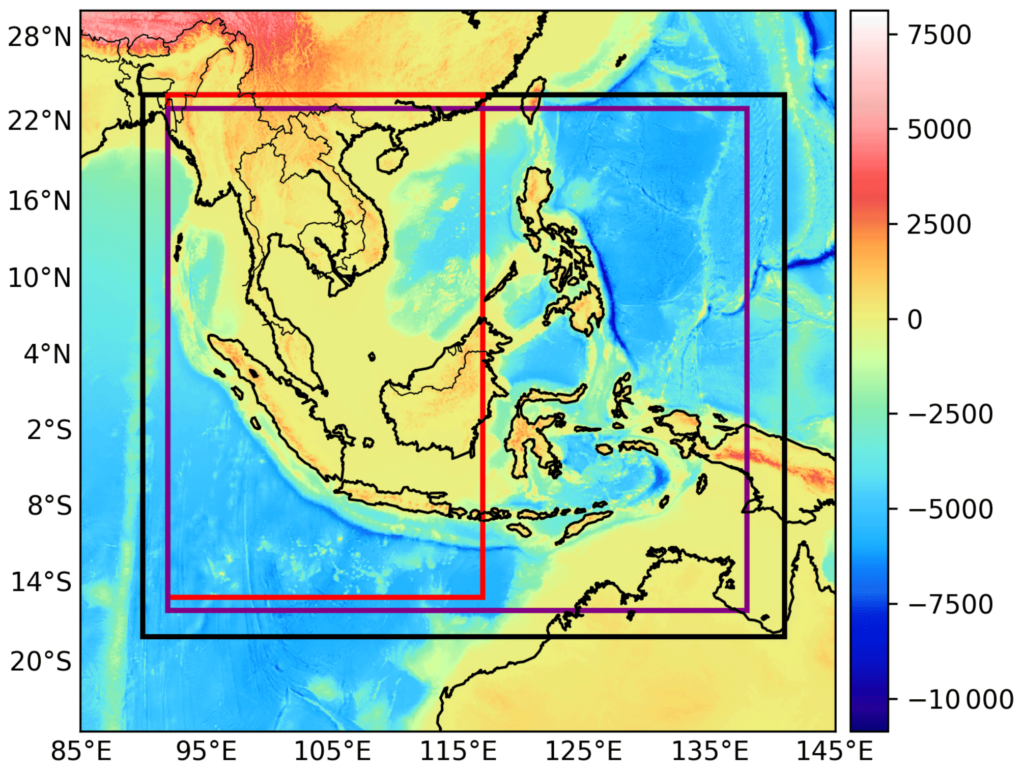
Figure 1 Bathymetry and orography (in metres) of the Maritime Continent from GEBCO 2014 data: MC coupled model domain (black box), western Maritime Continent domain in Thompson et al. (2018) (red box), and domain used for ocean forecast evaluation in present study (purple box).

The development of regional coupled models is mainly driven by the idea that by resolving fine-scale orographic, ocean circulation, and coastal ocean features, a more accurate representation of atmosphere–ocean dynamics and coupled processes can be achieved. The prediction of atmospheric and oceanic variables over the MC is challenging because of its complex geography, strong air–sea coupling, and remote ocean influences. Earlier studies suggested that the accuracy of atmospheric and ocean hindcast and forecast significantly improves when the simulations are performed using coupled models (Xue et al., 2014; Thompson et al., 2018; Lewis et al., 2019a). There have been a few coupled modelling studies over the MC focusing on the climate and weather research or short-range atmosphere–ocean forecasting (e.g. Aldrian et al., 2005; Wei et al., 2014; Li et al., 2017; Thompson et al., 2018). Recently, Xue et al. (2020) presented a review of atmosphere–ocean coupled modelling studies over the MC region.

Besides coupling, the model skill in simulating atmosphere and ocean state shows a strong relation to the grid resolution also (e.g. Li et al., 2017). Local mesoscale processes (e.g. land and sea breezes) also play an important role in the adequate simulation of upscale processes such as the MJO (Birch et al., 2016). Convection plays a fundamental role, either locally or embedded in bigger envelopes such as the MJO, influencing the diurnal cycle of precipitation and moving squall lines (Love et al., 2011). Therefore, the simulation of weather and climate processes over the MC requires sufficient resolution to resolve these scales and their interactions. Generally, a horizontal resolution of approx. 4 km, so-called convection permitting, has been effective in representing fine-scale processes over the MC (Love et al., 2011; Birch et al., 2014, 2016; Vincent and Lane, 2017). The first attempt towards the development of a convection-permitting atmosphere–ocean coupled model over the MC was undertaken by Thompson et al. (2018, hereafter T18). T18 used a regional version of the UK Met Office Unified Model (MetUM) atmospheric model and Nucleus for European Modelling of the Ocean (NEMO) ocean model configured for the western MC (WMC). For simplicity, the WMC coupled model configuration used in T18 is referred to as WMC_ao hereafter. The atmosphere and ocean components of WMC_ao were configured for the same domain and similar horizontal resolution of 4.5 km × 4.5 km (Fig. 1). The model resolution is fine enough to represent the complex coastal geography, ocean bathymetry at shallow oceans and straits, and orographic features, such as mountain ranges, with enormous influences in local weather (e.g. Bukit Barisan in Sumatra or the Sierra Madre in Luzon).

Work to develop and perform a first-hand evaluation of the WMC_ao, described in T18, was a preliminary step aimed to establish a high-resolution atmosphere–ocean coupled model focusing on the Southeast Asian region for both operational forecasts and climate research applications. Since the overall objective of the development was to simulate both atmospheric and oceanic variables, the coupling has provided a better consistency between the atmospheric conditions and that of the ocean underneath rather than employing stand-alone models. The case studies conducted as part of the WMC_ao evaluation suggested that the zonal extent of the domain might not be sufficient for an accurate prediction of weather events such as cold surges or typhoons. For instance, cyclogenesis inside the South China Sea (SCS) is relatively low and most of the cyclones and typhoons that appear over the SCS originated in the northwestern Pacific Ocean (e.g. Ling et al., 2011). The northern Pacific Ocean region between 100^∘ E and 180^∘E/W is the most active tropical cyclone basin on Earth and it accounts for about one-third of the world's tropical cyclones annually (e.g. Lee et al., 2020). Hence, rather than internally coupled dynamics, the predicted track and typhoon characteristics are dominantly driven by the lateral boundary conditions (LBCs) in WMC_ao. Similarly, the simulation of MJO- and cold-surge-related weather parameters may also be heavily influenced by LBCs. Hence, to address the issues encountered in T18 and incorporate the latest model scientific developments, the present study aims to bring several key upgrades to the WMC_ao configuration, and test its feasibility in operational forecast application. The main updates to the coupled modelling system include extending the eastern boundary of the model domain to the western Pacific Ocean, upgrading MetUM to the latest science configuration, and incorporating tide boundary forcing into the NEMO.

This study presents details of the atmosphere–ocean coupled prediction system developed for the MC and an evaluation of the ocean forecast from the system using a 6 d pre-operational forecast for October 2019. Following the method employed in many earlier coupled modelling studies (e.g. Li et al., 2014; Lewis et al., 2018), the evaluation of WMC_ao in T18 has been performed by using short case study simulations of selected weather events spanning over 5 d . In the present study, instead of case studies, we assess surface and subsurface oceanic variables predicted by the coupled system across different forecast lead times.

The next section of this paper presents an overview of the model setup, including a brief description of the model domain, atmospheric, ocean, and coupled model configurations. A brief discussion of the pre-operational forecast system setup is also presented. Section 3 provides the details of datasets used for the atmosphere and ocean model forcing and evaluation. Section 4 presents an assessment of the sea surface variables simulated by the stand-alone ocean model and both surface and subsurface ocean forecasts delivered by the MC coupled model. Finally, Sect. 5 summarises the results obtained from the study and suggests future developments.

2 Model setup

2.1 Model domain

The model domain extends from 18^∘ S to 24^∘ N and 92 to 141^∘ E (Fig. 1) on a regular latitude–longitude grid that covers most of the tropical regions of eastern Indian Ocean and western Pacific Ocean. The deepest oceanic trench on Earth, known as the Mariana Trench, is located in the northwestern Pacific Ocean. The crescent-shaped trench is positioned roughly between 10^∘ N, 140^∘ E and 60^∘ N, 150^∘ E (Gvirtzman and Stern, 2004). The model eastern boundary is limited to 141^∘ E to avoid numerical instabilities that may arise due to steep bathymetric slopes such as the Mariana Trench. Both the atmospheric and ocean components of the coupled system are selected to have the same domain. The horizontal resolution of the MC coupled model remained the same (4.5 km × 4.5 km) as that of the WMC_ao. The MC atmosphere–ocean coupled model configuration is referred to as MC_ao in this paper.

2.2 Atmospheric model

The atmospheric component of T18 has been improved to employ the SINGV v5 science configuration described in Huang et al. (2019), which is similar to the Regional Atmosphere and Land v1 in the Tropics (RAL1-T) configuration of MetUM (version 11.1) described in Bush et al. (2020). The model has been employed operationally by the Meteorological Service of Singapore since 2019 at a higher resolution (1.5 km) for the region 6^∘ S to 8^∘ N, 95^∘ E to 109^∘ E and is referenced in the literature as SINGV. The key differences of MC_ao atmospheric model component to T18 are as follows.

• Lateral boundary conditions are provided at 3-hourly frequency from the deterministic ECMWF forecasts instead of the MetUM global deterministic model. This change has led to a significant increase in precipitation skill scores across all spatial scales and precipitation thresholds in SINGV (Huang et al., 2019).

• The model uses a prognostic cloud fraction and prognostic condensate scheme (PC2, Wilson et al., 2008) instead of the diagnostic scheme of Smith (1990). This change helped to reduce the occurrence of spurious convection with very high rainfall rates and resulted in a better organisation of convection, as shown in Dipankar et al. (2020).

The rest of the model formulations are similar to T18 and the SINGV configuration described in Huang et al. (2019). The main characteristics of the model are summarised below.

• The dynamical core is the non-hydrostatic semi-Lagrangian and semi-implicit Even Newer Dynamics for the General Atmospheric Modelling of the Environment (ENDGAME, Wood et al., 2014), with an Arakawa-C staggered grid. The model time step is 120 s.

• The model has a terrain-following vertical coordinate with a resolution of 80 levels and a top lid at 38.5 km. The vertical resolution is 5 m at the boundary layer and 1.45 km below the model top, similar to the SINGV configuration.

• The boundary layer parameterisation is based on a blending between the one-dimensional scheme of Lock et al. (2001) and the three-dimensional Smagorinsky–Lilly scheme (Lilly, 1962); this blending is described in Boutle et al. (2014).

• The microphysics scheme is based on Wilson and Ballard (1999) with prognostic rain formulation and improved particle size distribution for rain as in Abel and Boutle (2012).

• The radiation scheme is based on the Edwards and Slingo (1996) scheme, with six bands in the shortwave and nine bands in the longwave (Manners et al., 2011).

• The Joint UK Land Environment Simulator (JULES, Best et al., 2011) land surface scheme with 9 surface fraction types is also used.

• The moist conservation scheme is used as described in Aranami et al. (2015).

The Atmospheric component of the MC_ao employed in this study is referred to as MCA_ao hereafter.

2.3 Ocean model

A regional version of Océan Parallélisé ocean engine within the NEMO (version 3.6_stable, revision 6232, Madec et al., 2016) framework is employed as the oceanic component of the MC_ao. NEMO is a primitive-equation, hydrostatic, Boussinesq ocean model extensively used in climate and operational forecast applications. The MC_ao ocean configuration shares many features of its predecessor, WMC_ao. Hence, only key features of the NEMO and main updates of MC_ao configuration are discussed here.

The model horizontal grid is in orthogonal curvilinear coordinates, with Arakawa-C grid staggering. The bathymetry of MC_ao is based on the General bathymetric Chart of the Oceans (GEBCO2014) 30 arcsec data (https://www.gebco.net/data_and_products/historical_data_sets/#gebco_2014, last access: 9 December 2020). The model has 51 vertical levels in terrain-following coordinate system and uses the stretching function by Siddorn and Furner (2013). The stretching function maintains a near-uniform surface cell thickness (≤1 m) and hence ensures the consistent exchange of air–sea fluxes over the domain, which is critical in the atmosphere–ocean coupling. Non-linear free surface following the variable volume layer formulation by Levier et al. (2007) is used for model free surface computation. The ocean model configurations used in our study have baroclinic and barotropic time steps of 120 and 8 s, respectively.

The generic length scale (GLS) turbulence model (Umlauf and Burchard, 2013) with K-ε turbulent closure scheme and the stability function from Canuto et al. (2001) are used to compute the turbulent viscosities and diffusivities. Background vertical eddy viscosity and eddy diffusivity coefficients are set to a lower value of 1.2 × 10⁻⁶ in MC_ao, whereas these coefficients were 1.2 × 10⁻⁴ and 1.2 × 10⁻⁵, respectively, in the WMC_ao. Additional vertical mixing resulting from internal tide breaking is parameterised in the model as proposed by St. Laurent et al. (2002). Both energy- and enstrophy-conserving schemes is used for the momentum advection. For lateral tracer diffusion, the Laplacian operator along geopotential levels with a coefficient of 20 m² s⁻¹ is used, while iso-level bi-Laplacian viscosity with a coefficient of −6 × 10⁷ m² s⁻¹ is applied for the momentum mixing. An implicit form of non-linear parameterisation with a log layer formulation is used for the bottom drag coefficient computation. The minimum and maximum of the drag coefficient are set to 0.0001 and 0.15, respectively.

At the lateral open-ocean boundaries, the flow relaxation scheme (FRS, Davies, 1976) is applied for the tracers and baroclinic velocities, while Flather boundary condition (Flather, 1976) is used for the sea surface height (SSH) and barotropic velocities. One of the key updates to MC_ao is the implementation of tide forcing at the lateral boundaries and tide potential at the ocean surface. Due to certain numerical issues, the tide-related forcings are not included in the WMC_ao. The tidal elevations and currents from finite-element solutions (FES2014b) data have been used for providing the tidal harmonics at the lateral boundaries (Lyard et al., 2006). A total of 15 major tidal constituents (Q1, O1, P1, S1, K1, 2N2, Mu2, Nu2, N2, M2, L2, T2, S2, K2, and M4) are included in the boundary forcing.

Both coupled and uncoupled ocean model configurations are employed in the study. For uncoupled simulations, the air–sea heat fluxes are estimated using the Common Ocean-ice Reference Experiment (CORE) bulk formulae (Large and Yeager, 2004). However, a direct flux formulation is used in the coupled ocean model. Monthly runoff climatology from Dai and Trenberth (2002) and chlorophyll monthly climatology from SeaWiFS satellite observation are provided as runoff forcing and to compute light absorption coefficients, respectively, in all ocean configurations. The red–blue–green (RGB) scheme is used to calculate the penetration of shortwave radiation into the ocean (Lengaigne et al., 2007). Identical to WMC_ao, the fraction of solar radiation absorbed at the surface layer is defined to be 56 % of the downward component. Mean sea level pressure (MSLP) forcing is included in the surface boundary forcing to take account of the inverse barometric effect on SSH.

The uncoupled and coupled ocean model configurations employed in this study are referred to as MCO and MCO_ao, respectively.

2.4 Coupled configuration

The exchange of fluxes between the atmosphere and ocean models is achieved through the Ocean Atmosphere Sea Ice Soil coupler (version 3.3) interfaced with the Model Coupling Toolkit (OASIS3-MCT) libraries (Valcke, 2013). The Earth System Modelling Framework (ESMF) regrid tools are used to generate the interpolation weights for the remapping of exchange fields. The coupling occurs at hourly frequency, and hourly mean fields are exchanged. Since a direct flux formulation is implemented, the heat fluxes computed using the Monin–Obukhov similarity theory is exchanged from the atmosphere to the ocean model. The sea surface temperature (SST) and zonal and meridional surface current fields are sent from the ocean to the atmosphere model. The variables exchanged from atmosphere to the ocean include non-solar heat flux, net shortwave radiation, liquid precipitation, net evaporation, and zonal and meridional wind stress. Due to numerical issues, MSLP exchange from the atmosphere is not enabled in the MC_ao. Instead, it is supplied from an external data source to the ocean model. The MSLP from ECMWF IFS data have been used in our coupled forecast simulations.

2.5 Model initialisation and forcing

To assess the performance of the ocean model and provide initial condition to the MCO_ao, a 69-month hindcast simulation is performed with MCO for the period 1 January 2014 to 30 September 2019. The MCO was initialised in 1 January 2014 using temperature, salinity, zonal and meridional currents, and SSH derived from Mercator global ocean reanalysis. The lateral boundary condition for the hindcast simulation is also obtained from the same ocean reanalysis data. The daily mean of temperature, salinity, baroclinic and barotropic velocities, and SSH are included in the lateral boundary forcing. Ocean surface is forced by ECMWF Reanalysis 5 (ERA5) during the period from 1 January 2014 to 30 June 2019. Downward shortwave and longwave radiation at the ocean surface; total precipitation; MSLP; and 10 m wind velocities, air temperature, and specific humidity fields are included in the forcing file. Since there was a delay of about 2–3 months in the release of ERA5 data during the time of model development, the MCO is forced by the 6-hourly ECMWF IFS analysis fields from 1 July 2019 to the start of MC_ao pre-operational forecast run on 1 October 2019 (Fig. 2a). As the atmospheric adjustments are sub-daily, no spin-up or hindcast simulations are performed for the MCA_ao.

Figure 2 Schematic of modelling systems used in the study: (a) MC ocean-only model (MCO) hindcast and (b) MC atmosphere–ocean coupled forecast model (MC_ao). MCO_ao stands for the MC coupled ocean model, MCA_ao stand for the MC coupled atmospheric model, LBC stands for the lateral boundary condition, SBC stands for the surface boundary condition, IC stands for the initial condition.

A schematic of the atmosphere–ocean coupled system used in the pre-operational forecast is shown in Fig. 2b. In the coupled prediction system, the MCA_ao is initialised daily at 00:00 Z UTC from the ECMWF IFS analysis. MCO run for the previous day (T0 minus 1), forced by 6-hourly ECMWF IFS analysis at the surface and the daily mean of updated Mercator ocean forecast as the LBC, provides the initial condition to MCO_ao. Since it is driven by analysed (or updated) surface (lateral) boundary conditions, the MCO provides an updated initial condition to the MCO_ao daily. The MC_ao forecast run is driven by LBC from 3-hourly ECMWF IFS forecasts in the atmosphere and daily Mercator forecasts in the ocean. Since the MSLP from MCA_ao is not incorporated in MCO_ao, 3-hourly EMCWF IFS forecast data are supplied to the model.

2.6 Pre-operational forecast setup

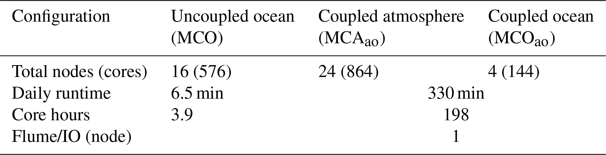
The atmosphere–ocean coupled forecast model ran as a pre-operational forecast system from 1 to 31 October 2019 at the Cray XC-40 HPC located in the Center for Climate Research Singapore (CCRS), Singapore. The forecast system includes all necessary programs and scripts for the pre-processing of atmospheric and oceanic variables to their respective model grids. The forecast system is scheduled to initialise the forecasts daily at 13:00 UTC, and simulations are completed by ∼ 18:40 UTC. Summary of HPC resources usage and typical runtimes for daily forecast simulations are shown in Table 1. To minimise the output size, only basic oceanic and atmospheric variables are included in the output. The forecast from MCO_ao includes instantaneous SSH; hourly averaged sea surface temperature, sea surface salinity, and surface current velocities; and the daily mean of ocean temperature, salinity, and ocean currents. Further, to test the feasibility of the coupled forecast system for operational purpose, we have conducted simulations with increased computational resources. Test simulations showed that by increasing the computational resources to 81 nodes (2916 cores), the total runtime has been reduced to ∼ 140 min. This suggests a near-linear reduction in total runtime with an increase in computation nodes.

Table 1 Summary of HPC resources usage and typical runtimes.

3 Data

A brief description of the reanalysis, forecast, and observational datasets used for the model initialisation, forcing, and evaluation is presented in this section.

3.1 Model initialisation and forcing

ERA5 is a climate reanalysis produced by the ECMWF providing hourly estimates of many atmospheric, land, and oceanic fields (Hersbach et al., 2020). Currently, it covers the period from 1979 to within 5 d of the present, and its horizontal resolution is approx. 30 km. The reanalysis is produced using 4D-Var assimilation of the ECMWF Integrated Forecast System (IFS). ERA5 combines vast amounts of historical observations into global estimates using advanced modelling and data assimilation systems. The data are freely available through the data server https://cds.climate.copernicus.eu/ (last access: 20 November 2020).

ECMWF IFS is a global weather prediction system comprising a spectral atmospheric model, ocean wave model, ocean model, and land surface model coupled to a 4D-Var data assimilation system. IFS medium-range weather forecasts are available up to 10 d at a horizontal resolution of 0.1^∘. In addition, the atmospheric analysis fields are provided four times daily for the forecast base times 00:00, 06:00, 12:00, and 18:00 UTC. The data are available to registered users from https://www.ecmwf.int/en/forecasts/datasets/ (last access: 20 November 2019).

Mercator global ocean reanalysis and forecast provides oceanic variables with 0.0833^∘ horizontal resolution (Lellouche et al., 2018). The system uses NEMO v3.1 with 50 vertical z levels ranging from zero to 5500 m and forced by the ECMWF IFS meteorological variables. The assimilation and forecast product includes the daily mean of temperature, salinity, currents from top to bottom over the global ocean, and SSH. The data are freely available from https://marine.copernicus.eu/ (last access: 20 December 2020).

The tidal heights and currents computed from the global tide model finite-element solution (FES2014b) is used as the tidal forcing in the model. FES2014 is based on the resolution of the shallow water hydrodynamic equations (T-UGO model) in a spectral configuration and using a global finite-element mesh with increasing resolution in coastal and shallow waters regions (Lyard et al., 2006). The database is distributed on a global $\mathrm{0.0625}{}^{\circ }\times \mathrm{0.0625}{}^{\circ }$ grid. Data are produced by assimilating long-term altimetry data (Topex, Poseidon, Jason-1, Jason-2, TPN-J1N, and ERS-1, ERS-2, ENVISAT) and tidal gauges through an improved representer assimilation method. Tidal heights and currents of 32 tidal constituents are available. The data are freely available through http://www.aviso.altimetry.fr/en/data/products/auxiliary-products/global-tide-fes.html (last access: 25 November 2020).

3.2 Model evaluation

The CORIOLIS data service provides quality-controlled in situ data in real-time and delayed modes over the global ocean. The data include temperature and salinity profiles and time series from profiling floats, expendable bathythermographs (XBTs), thermo-salinographs (TSGs), and drifting buoys. The data are freely available from http://www.coriolis.eu.org/Data-Products/ (last access: 6 November 2020).

The Operational Sea Surface Temperature and Sea Ice Analysis (OSTIA) SST is produced daily on an operational basis at the UK Met Office using optimal interpolation on a global $\mathrm{0.054}{}^{\circ }\times \mathrm{0.054}{}^{\circ }$ grid. The product assimilates satellite data including advanced Very-High Resolution Radiometer, Spinning Enhanced Visible and Infrared imager, Geostationary Operational Environmental Satellite Imager, Infrared Atmospheric Sounding Interferometer, and Tropical Rainfall Measuring Mission Microwave imager data and in situ data from ships and drifting and moored buoys (Donlon et al., 2012). SST data at every grid point are accompanied by an uncertainty estimate, known as an analysis error, and an optimal interpolation approach is employed to produce this estimate. The data are freely available from https://marine.copernicus.eu/ (last access: 22 December 2020).

The University of Hawaii Sea Level Center (UHSLC) offers quality-controlled tide gauge (TG) sea level observations over the global ocean as fast-delivery (FD, 1–2-month delay) and research-quality (RQ, 1–2-year delay) data at hourly and daily resolution (Caldwell et al., 2015). The data are freely available from http://uhslc.soest.hawaii.edu/data/ (last access: 23 November 2020).

4 Results and discussion

An evaluation of the MCO hindcast and MCO_ao forecast simulations are presented in this section of the paper. Direct comparison of model simulations with observation or analysis data has been performed. Based on the availability of in situ or satellite observation at the time of data analysis, only a few variables are selected for assessing the model performance. In addition, to maintain consistency between the evaluation of hindcast and forecast simulations, analyses of the same set of variables and observation data have been performed where possible. Oceanic variables employed for the evaluation are SST, SSH, and the subsurface temperature and salinity. Model hindcasts and forecasts over the region 16^∘ S to 23^∘ N and 92 to 138^∘ E and defined as the analysis domain (Figs. 1 and 3), is further used for the analysis. The MC model domain includes oceanic basins with different geographical and climatological characteristics. For the evaluation purpose, we have divided the analysis-domain into 10 sub-regions based on their geographical distribution (Fig. 3). These sub-regions are the (1) Andaman Sea–Malacca Strait (ASMS), (2) southern South China Sea (SSCS), (3) Gulf of Thailand (GoT), (4) the rest of the South China Sea (RSCS), (5) the tropical western Pacific Ocean (TWPO), (6) Sulu–Celebes seas (SuCeS), (7) Banda Sea (BS), (8) Java Sea (JS), (9) Timor–Arafura seas (TAS), and (10) the tropical eastern Indian Ocean (TEIO).

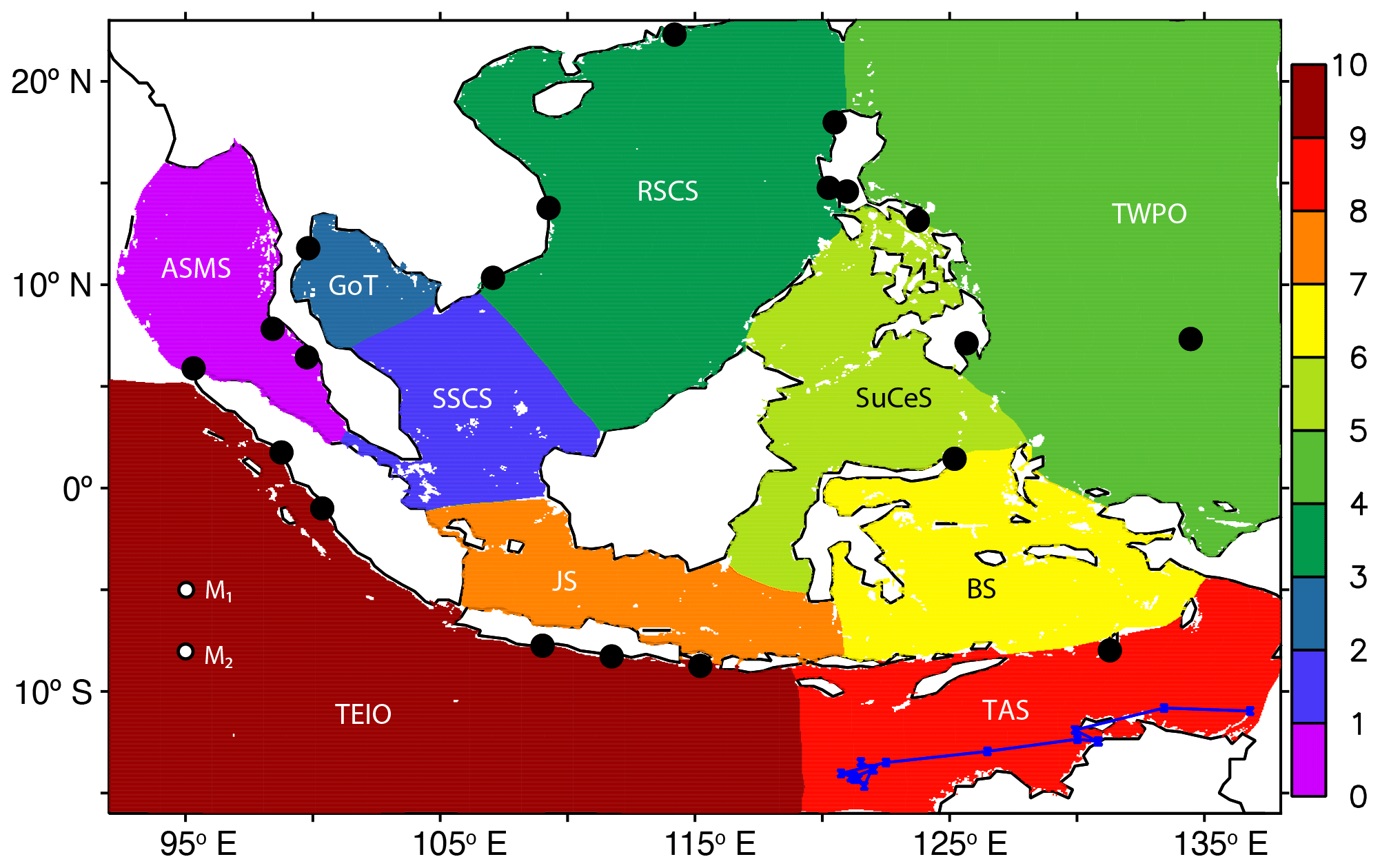
Figure 3 Domain used for hindcast and forecast evaluation with sub-regions defined in the study: (1) Andaman Sea–Malacca Strait (ASMS), (2) southern South China Sea (SSCS), (3) Gulf of Thailand (GoT), (4) the rest of the South China Sea (RSCS), (5) the tropical western Pacific Ocean (TWPO), (6) Sulu–Celebes seas (SuCeS), (7) Banda Sea (BS), (8) Java Sea (JS), (9) Timor–Arafura seas (TAS), and (10) the tropical eastern Indian Ocean (TEIO). The Bay of Bengal region (north of 5^∘ N, west of 92^∘ E) is excluded when analysis is performed for different sub-regions. The blue line in the TAS indicates the TSG observation track. The locations of tide gauges are shown as black circles. Moored buoy locations M₁ (5^∘ S, 95^∘ E) and M₂ ( 8^∘ S, 95^∘ E) are also shown.

4.1 Ocean hindcast

An overall assessment of the ocean model hindcast simulation is carried out to understand the realism of the ocean initial condition for the coupled forecasts, particularly at the ocean surface where the exchange of fluxes between the atmosphere and ocean takes place. Though the hindcast simulations encompass from 1 January 2014 to 30 September 2019, we only evaluate ERA5-driven simulations during the period from 1 January 2018 to 30 June 2019. The first 4 years of the simulation data are considered the spin-up stage of the model. Comparison of daily mean SST with OSTIA analysis and moored buoys observations is presented, while the daily mean SSH is compared with tide gauge observations. Moored observation buoys in the eastern tropical Indian Ocean established as part of the Research Moored Array for African–Asian–Australian Monsoon Analysis (RAMA, McPhaden et al., 2009) at the locations 5^∘ S, 95^∘ E (M₁) and 8^∘ S, 95^∘ E (M₂) are used for the evaluation. Fast-delivery (FD) data from UHSLC for 20 tide gauge stations are employed for the SSH comparison.

4.1.1 Sea surface temperature

Comparison of model-simulated daily mean SST with OSTIA analysis is shown in Fig. 4. Spatial distribution of model SST bias (Fig. 4a), root-mean-square difference (RMSD) (Fig. 4b), correlation coefficient (Fig. 4c) and the spatial average of SST difference over the analysis domain (Fig. 4d) are given. Model performance in simulating SST over the sub-regions is given in Table 2. SST Bias, RMSD, and correlation coefficient statistics computed using modelled SST and OSTIA are shown in Table 2. The SST bias is within ±0.2 ^∘C for about 76 % of the analysis domain and within ±0.5 ^∘C for about 98 % of the analysis domain. The largest SST cold bias is seen in the Andaman Sea region. Meanwhile, most of the South China Sea (SCS), equatorial western Pacific Ocean, and the Australian coast of the Timor Sea show a positive SST bias. Negative SST bias of about −0.25 ^∘C is observed in the ASMS region, while positive bias over 0.25 ^∘C is confined to the SSCS and GoT sub-regions. Rather than appearing as a basin-wide feature, higher positive biases appear as small circular patches in the northern SCS region that represent the likely existence of cyclonic eddies over this region.

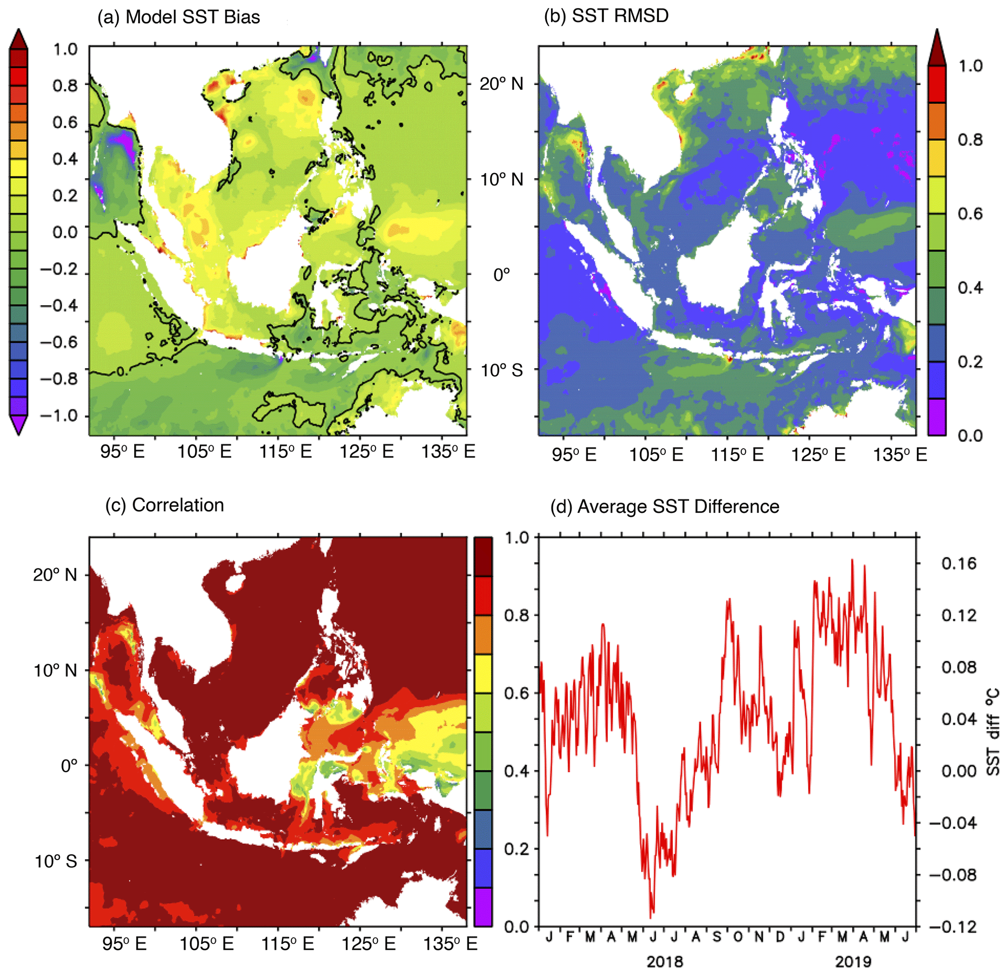
Figure 4 Spatial distribution of daily averaged (a) SST bias (^∘C), (b) RMSD (^∘C), and (c) correlation coefficient between the MCO hindcast and OSTIA analysis. (d) Spatial average of SST difference between the model and OSTIA over the analysis domain (^∘C).

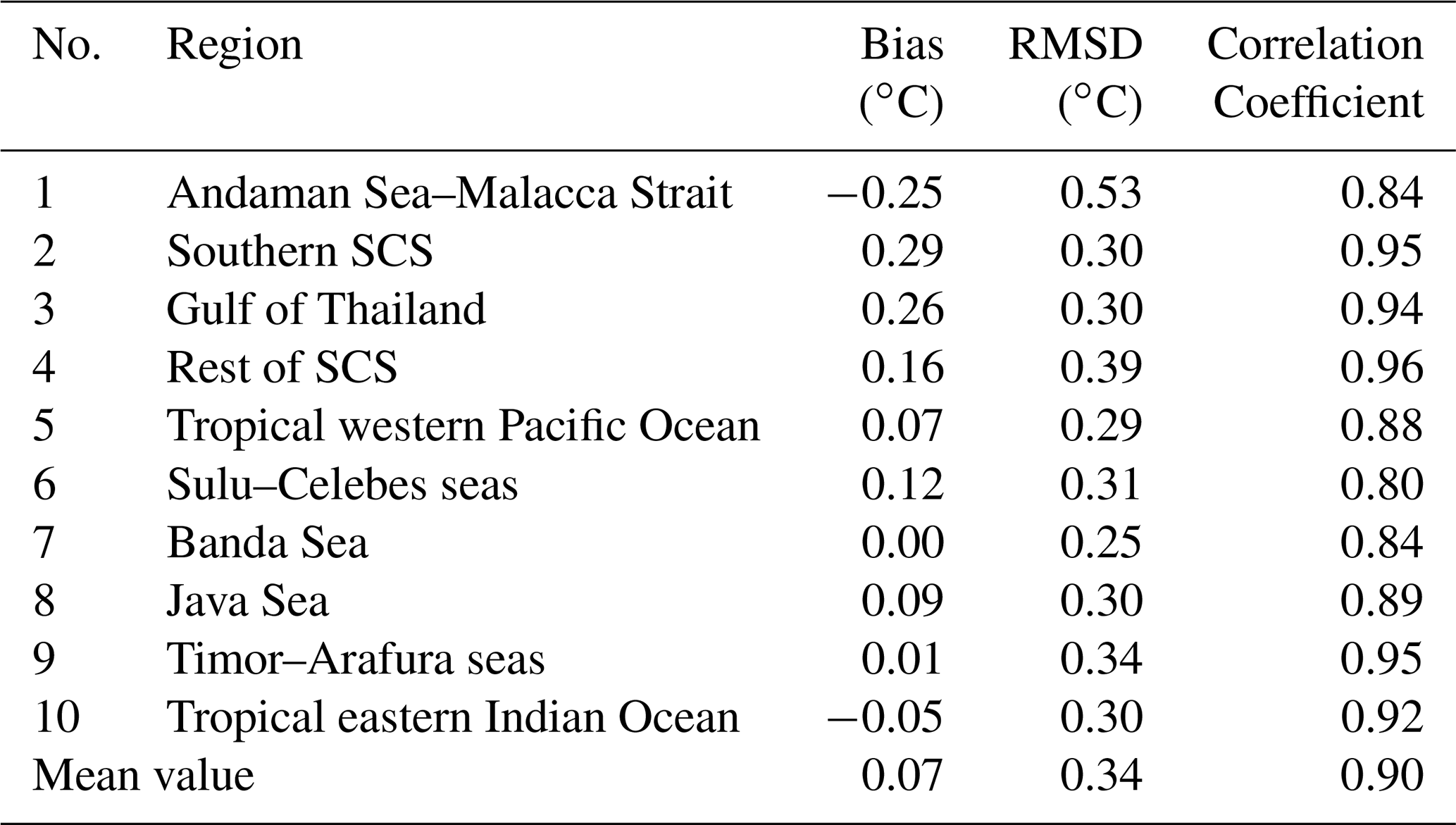
The RMSD between the model and OSTIA is less than 0.5 ^∘C for about 97 % of the analysis domain (Fig. 4b). Small patches of higher RMSD (> 0.7 ^∘C) are mostly seen along the coastal regions. The RMSD minimum (0.25 ^∘C) and maximum (0.53 ^∘C) are observed over the BS and ASMS sub-regions, respectively (Table 2). Correlation between the model SST hindcast and OSTIA is above 99.9 % confidence level over the analysis domain (Fig. 4c). Over 88 % of the domain displays a correlation higher than 0.8. Relatively low correlation is seen over the middle of the Malacca Strait, Makassar Strait, and equatorial Pacific Ocean regions. In sub-region spatial average, the lowest (0.8) and highest (0.96) correlations are seen over the SuCeS and RSCS regions, respectively (Table 2). Time series of the spatially averaged SST difference between the model and OSTIA is shown in Fig. 4d. Consistent with our earlier analyses, relatively low SST difference depicts a good agreement between the MCO SST hindcast and OSTIA analysis. Further analysis of SST in different sub-regions revealed that relatively higher SST over the GoT, SSCS and SuCeS regions contribute to the positive SST differences during February–April in 2018 and 2019 and September–October in 2018 (figures not shown). Meanwhile, SST simulation over those sub-regions shows improvement during June–July 2018. Higher negative SST bias over the ASMS region mainly contributes to the negative SST difference during the same period. Overall, the mean SST bias, RMSD, and mean correlation over the analysis domain are 0.07 ^∘C, 0.34 ^∘C, and 0.90, respectively.

Table 2 Summary of SST bias, RMSD, and correlation coefficient statistics between the model hindcast and OSTIA for the period 1 January 2018 to 30 June 2019. Daily mean SST from the model and OSTIA is used for the analysis.

The time series of daily mean SST from the RAMA moored observation buoys located in the southeastern tropical Indian Ocean at 5^∘ S, 95^∘ E (M₁) and 8^∘ S, 95^∘ E (M₂) is shown in Fig. 5. Model SST is bilinearly interpolated to the buoy locations. Temperature observations at 1 m depth are taken as SST from the moored buoys, while temperature averaged over the upper 1 m is indicated as the model SST at these locations. In general, a good agreement is found between the model and observations at both mooring locations. Both the seasonal and intra-seasonal SST variability are reasonably well reproduced by the model. SST bias, RMSD, and correlation between the model and observation are 0.17 ^∘C, 0.29 ^∘C, and 0.94, respectively, for M₁ and 0.12 ^∘C, 0.41 ^∘C, and 0.92, respectively, for M₂. The standard deviation (SD) of SST at M₁ and M₂ are 0.94 ^∘C and 0.99 ^∘C, respectively, and the RMSD is smaller than the SD at both locations.

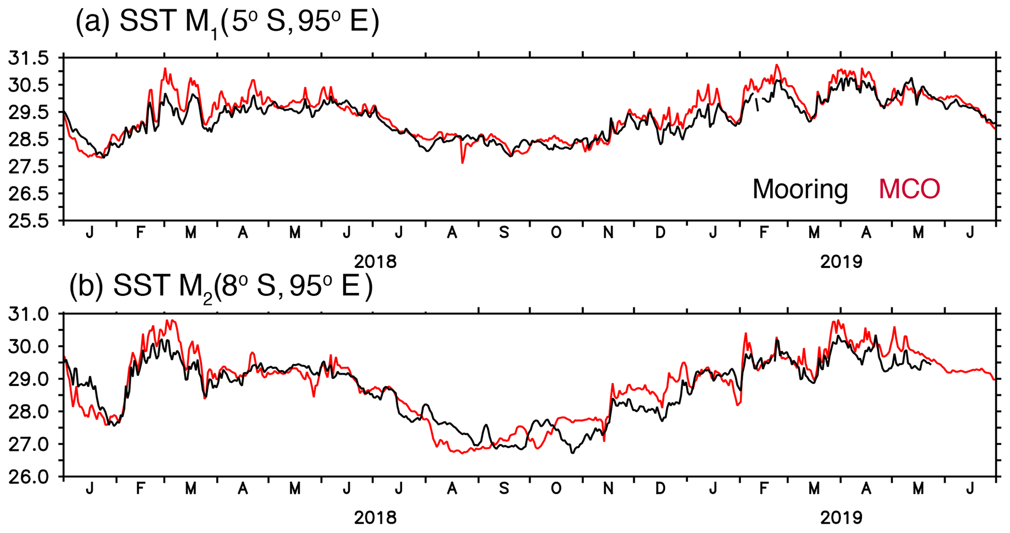
Figure 5 Comparison of daily averaged SST from MCO hindcast and RAMA moored buoys at (a) M₁ and (b) M₂ during the period 1 January 2018 to 30 June 2019.

4.1.2 Sea surface height

Daily mean SSH observation from 20 tide-gauge stations distributed across the domain and MCO simulated SSH interpolated to the location of these observations have been used for the hindcast evaluation. SSH bias, RMSD and correlation coefficient statistics between model and SSH observations are given in Table 3. Highest SSH bias (0.12 m) and RMSD (0.15 m) are seen at the Malakal, Palau, tide gauge station. The SSH bias is within ±0.05 m for 17 of the total 20 stations analysed. The model accuracy is higher than 0.10 m for 18 stations, while 14 of the total 20 stations have an accuracy greater than 0.05 m. The SSH correlation between the model and observations is above 99.9 % confidence level for all tide gauge stations employed in the analysis. The correlation is above 0.80 for 16 tide gauge stations. Lowest correlation of 0.60 is observed at the Malakal tide gauge station. Mean SSH bias, RMSD, and mean correlation between the model and observation are 0.01 m, 0.06 m, and 0.87, respectively.

Table 3 Summary of SSH bias, RMSD, and correlation coefficient statistics between MCO hindcast and tide gauge stations for the period 1 January 2018 to 30 June 2019. Daily mean SSH from model and tide gauge is used for the analysis.

Time series of daily mean SSH from model and observations for randomly selected stations are plotted in Fig. 6. The stations Sibolga and Prigi are located in the eastern tropical Indian Ocean, and Currimao Ilocos Norte and Vung Tau are located in the SCS. Generally, the model-simulated SSH follows the observation and shows good agreement with it. A few sharp peaks in the tide gauge observation are found to be absent in the model simulation (e.g. Fig. 6c). Most of the tide gauge stations are located adjacent to the coast, and our current model resolution is not enough to resolve the coastline at very fine scales. Since the model SSH is interpolated to the tide gauge location, local-scale SSH variations may not be captured in the model simulation. This may be one possible reason for the discrepancy between the model and observations.

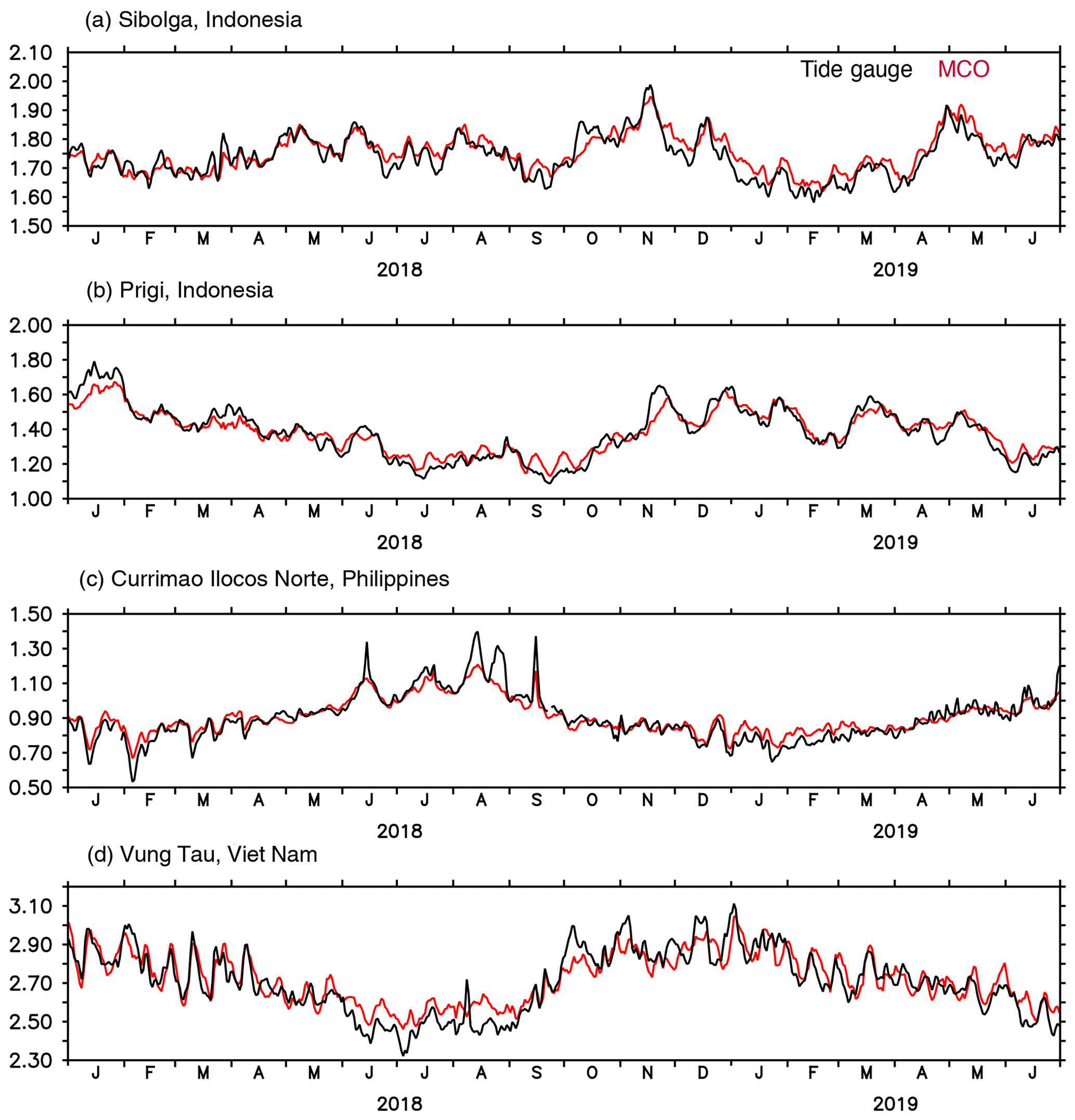
Figure 6 Time series of daily mean SSH (in metres) from tide gauge observations (black line) and MCO hindcasts (red line) at randomly selected stations, (a) Sibolga (1.75^∘ N, 98.76^∘ E), (b) Prigi (8.28^∘ S, 111.73^∘ N), (c) Currimao Ilocos Norte (17.988^∘ N, 120.488^∘ E), and (d) Vung Tau (10.34^∘ N, 107.072^∘ E), from 1 January 2018 to 30 June 2019.

Comparison of model-simulated SST and SSH fields shows good agreement with observation and analysis data. The RMSD and bias statistics of SST and SSH relative to the observation are within the acceptable error limits of ocean hindcast simulations (e.g. Yang et al., 2016). Statistically significant correlation with observation suggests that both the spatial and temporal patterns of variability are reasonably well reproduced by the model.

4.2 Ocean forecasts

Results from the analysis of MCO_ao forecast simulations for October 2020 are presented here. Since the system delivers a 6 d forecast, the analysis period extends from 1 October to 5 November 2020. Daily files are produced at different forecast lead times, T+0 to T+24 (fcst_day1), T+24 to T+48 (fcst_day2), T+48 to T+72 (fcst_day3), T+72 to T+96 (fcst_day4), T+96 to T+120 (fcst_day5), and T+120 to T+144 (fcst_day6) for the following analyses. Comparisons of coupled ocean forecasts for different forecast lead times with OSTIA SST and in situ observations have been performed, such as temperature from RAMA moored buoys, TSG, and XBT profiles; temperature and salinity from conductivity temperature depth (CTD) profiles; and SSH from tide gauges.

4.2.1 Sea surface temperature

Time series of daily mean SST averaged over the sub-regions from OSTIA analysis and different forecast lead times are plotted in Fig. 7. Statistics of SST bias, RMSD, and correlation coefficient between the model and OSTIA for the October forecast run are listed in Table 4. The forecasted SST over most of the sub-regions is within the error standard deviation of the OSTIA analysis, which is indicated by shading in Fig. 7. Excluding the ASMS, all other sub-regions exhibit a warm SST bias, with the largest values over the SSCS and GoT. The RMSD is less than 0.5 ^∘C over most of the sub-regions during the analysis period. Over the ASMS sub-region, both the cold bias and RMSD increase with the forecast lead time, and it shows the highest RMSD (0.49 ^∘C) on fsct_day6. The largest SST RMSD (0.56 ^∘C) and bias (0.49 ^∘C) over all sub-regions is observed over the GoT with a 1 d forecast lead time. Generally, the forecasted SST tends to be cooler, with an increase in forecast lead time denoting a lower warm bias and RMSD relative to fcst_day1. Interestingly, inconsistent with the improvements in SST bias and RMSD, the correlation between forecasted and OSTIA time series considerably decreases with higher forecast lead times (Table 4).

Table 4 Summary of SST bias and RMSD (a) and correlation coefficient (b) statistics between coupled ocean forecasts and OSTIA over the sub-regions shown in Fig. 3 from 1 to 31 October 2019. Daily mean SST from model and OSTIA is used for the analysis.

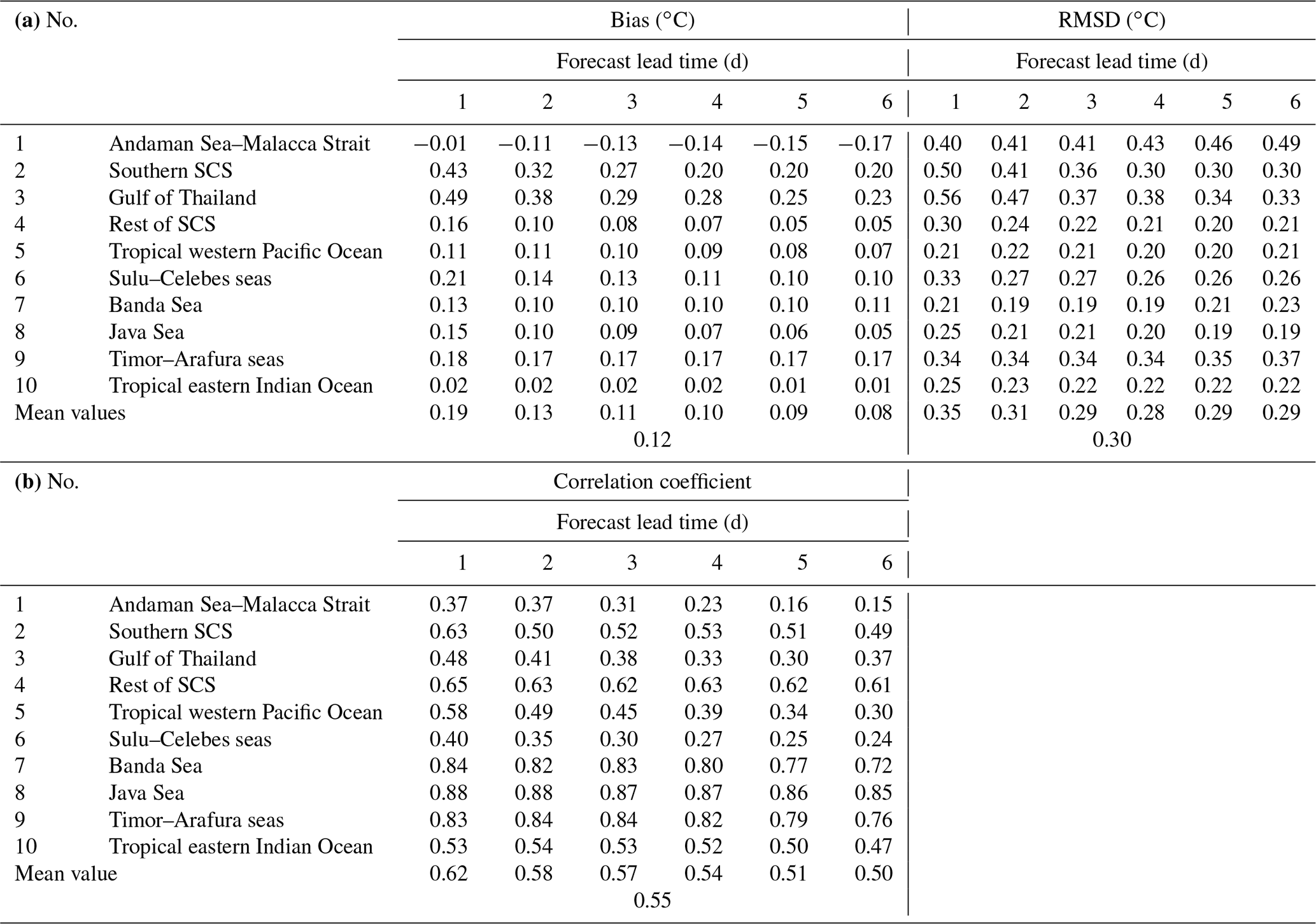
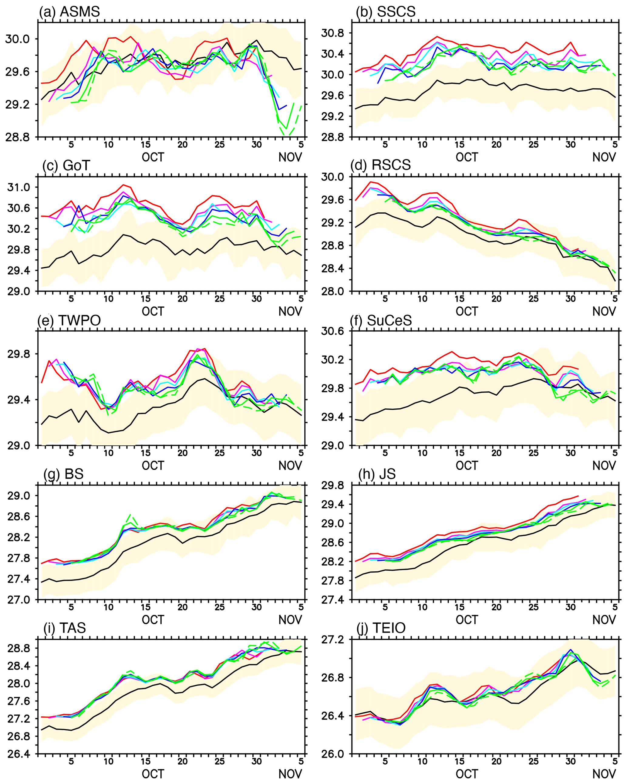
Figure 7 Time series of daily mean SST from model forecast and OSTIA averaged over the sub-regions: OSTIA (black line), fcst_day1 (red line),  fcst_day2 (purple line), fcst_day3 (light blue line), fcst_day4 (blue line), fcst_day5 (green line), and fcst_day6 (dashed green line). Shading represents the estimated error standard deviation of analysed SST in OSTIA. (a) ASMS stands for Andaman Sea–Malacca Strait, (b) SSCS stands for southern SCS, (c) GoT stands for Gulf of Thailand, (d) RSCS represents the rest of the SCS, (e) TWPO stands for tropical western Pacific Ocean, (f) SuCeS stands for the Sulu–Celebes seas, (g) BS stands for the Banda Sea, (h) JS stands for the Java Sea, (i) TAS stands for the Timor–Arafura seas, (j) TEIO stands for tropical eastern Indian Ocean. The y axes are differ between the plots.

SST correlation is above the 95 % confidence level (r > 0.365) over the entire analysis domain during fcst_day1. In general, SST correlation is higher than 99 % confidence level (r > 0.46) over 60 % of the sub-regions during higher forecast lead times as well. The sub-regions including ASMS, GoT, TWPO, and SuCeS are noted by lower correlation significance level with an increase in forecast lead time. Overall, the SST correlation over the analysis domain is above the 99 % confidence level across all forecast lead times, while bias and RMSD are less than 0.19 and 0.35 ^∘C, respectively.

Figure 8 shows the time series of hourly averaged SST at M₁ (Fig. 8a) and M₂ (Fig. 8b) mooring locations from observation and model forecasts. It should be noted that the observation at M₂ is available for a relatively short period from 21 October to 5 November 2020. Statistics of the SST bias, RMSD, and correlation coefficient between the model forecast and the observations are listed in Table 5. The diurnal variability of SST at both locations is reasonably well reproduced by the model in all forecast lead times. However, the model forecasts have overestimated the SST diurnal variations from 23 October 2019. SST cooling during late October–early August 2020 at the location M₁ is underestimated in the model forecast. SST bias and RMSD at M₁ are less than 0.07 and 0.20 ^∘C, respectively, and remain fairly constant across all forecast lead times. Despite this, the correlation between model forecasts and observations depicts a considerable decrease at higher forecast lead times. A cold SST bias of about −0.14 to −0.17 ^∘C is noted at location M₂. The RMSD at M₂ is relatively low, with a maximum of 0.18 ^∘C across all forecast lead times while compared to M₁. The SST correlation at M₂ is above the 95 % confidence level (r > 0.61, df ≥9) during all forecast lead times.

Table 5 Items (1) and (2) are a summary of SST bias and RMSD (a) and correlation coefficient (b) statistics between coupled ocean forecasts and observations at the mooring locations M₁ (5^∘ S, 95^∘ E) and M₂ (8^∘ S, 95^∘ E) during October 2019. Hourly averaged temperature from the model and observations is used for the analysis. Item (3) is the same as items (1) and (2) but for temperatures at 6.4 m depth along the track shown in Fig. 3. Daily averaged temperature from model and instantaneous temperature at 12:00 UTC from observation is used for the analysis. Item (4) is the same as items (1) and (2) but for temperatures within 0 to 600 m depth at the mooring location M₁. Daily averaged temperature model and observations used in the analysis.

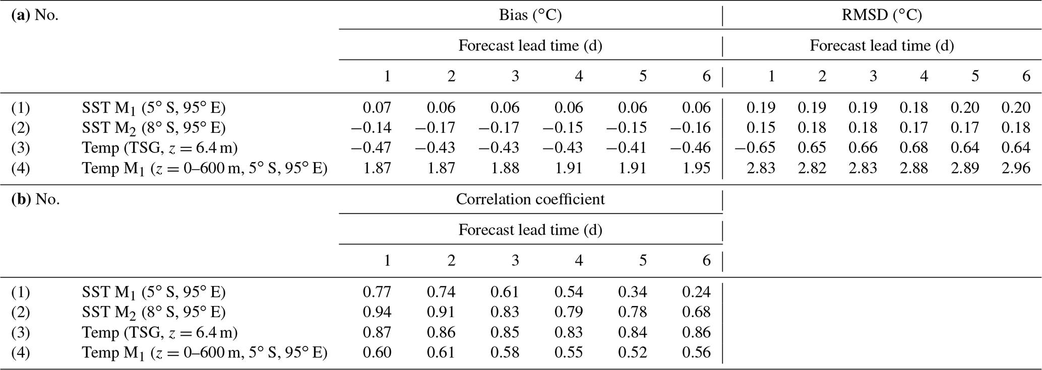
Figure 8 (a, b) Time series of hourly mean SST from model forecast and observations at the locations M₁ (5^∘ S, 95^∘ E) and M₂ (8^∘ S, 95^∘ E). Buoy locations are shown in Fig. 3. (c) Subsurface temperature at 6.4 m depth for track shown in Fig. 3 from TSG and model: observations (black line), fcst_day1 (red line), fcst_day2 (purple line), fcst_day3 (light blue line), fcst_day4 (blue line), fcst_day5 (green line), and fcst_day6 (dashed green line).

Table 6 Summary of temperature and salinity RMSD statistics between coupled ocean forecasts and in situ (Argo profile and XBT) observations from 1 October to 5 November 2019. Daily averaged temperature from the model and instantaneous temperature or salinity from observations are used for the analysis. Numbers in bold indicate the number of profiles analysed for each variable and lead forecast time.

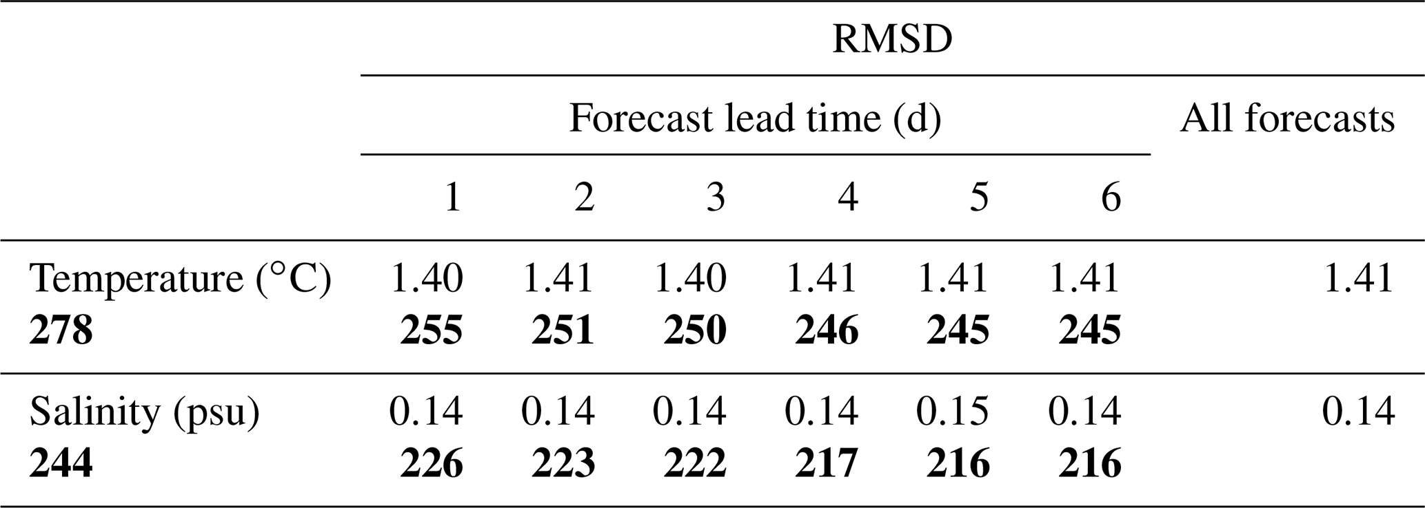
Table 7 Summary of SSH RMSD and bias statistics between coupled ocean forecasts and tide gauge observations during October 2019. Hourly instantaneous SSH from the model and observations is used for the analysis.

4.2.2 Temperature and salinity

Temperature and salinity data available from the CORIOLIS data portal are employed for the MCO_ao forecast evaluation of subsurface fields. Argo and XBT profiles, moored buoys, and TSG observations are used for the analysis. We only consider mooring and TSG observations with a minimum of 10 d for the analysis. TSG observation selected for the analysis is located in the Timor and Arafura seas, and the track has a direction of motion towards the west (Fig. 3). Continuous observations available at 6.4 m depth are compared with the model forecasts. Currently, the forecast system produces only daily averaged subsurface variables. Hence, the instantaneous TSG temperature observations at 12:00 UTC are compared with the daily averaged model temperature. Time series of TSG temperature observations and model forecasts for different forecast lead times are shown in Fig. 8c. Though the model temperature shows a negative bias, daily temperature variation is reasonably well predicted by the model. This is supported by the high correlation, above the 99.9 % confidence level, between the model forecast and observation (Table 5, item 3). The largest temperature bias and RMSD are −0.47 ^∘C and 0.68 ^∘C, respectively, and significant variations in bias, RMSD, and correlation statistics are not noticeable.

The moored buoy observations provide a unique opportunity to assess the model simulations both in the surface and subsurface of the ocean. Since the variables of interest in the present study are temperature and salinity, we have tried to compare the model forecast of temperature and salinity with buoy observation available at the locations M₁ and M₂. However, due to data gaps and shorter time series, salinity observation from both moorings and temperature from M₂ mooring are not included in the analysis. Depth–time plots of temperature from the model for forecast lead times 1 d (fcst_day1), 3 d (fcst_day3), and 5 d (fcst_day5) and the moored observation (M₁) are shown in Fig. 9. Statistics of temperature bias, RMSD, and correlation coefficient between the model forecast and observations are given in Table 5. The depth of the upper ocean isothermal and mixed layer and its shoaling in late October are well simulated by the model. A significant difference between the model forecast and observations is seen in the region below the mixed layer. The model simulation is unable to reproduce the sharp temperature stratification and cooling in the thermocline regions, while this feature is clearly evident in the observations. This leads to a relatively large discrepancy between the model and observation in the subsurface region roughly between 100 to 250 m depths. The usage of daily averaged temperature rather than instantaneous profile or higher vertical mixing in the model may be one of the possible reasons for this discrepancy. Larger temperature differences at the thermocline region have led to a warm temperature bias in the model forecast (Table 5). Maximum temperature bias and RMSD are 1.95 and 2.96 ^∘C, respectively. Meanwhile, the correlation between the model forecast and observation is above the 99 % confidence level (r > 0.47) across all forecast lead times.

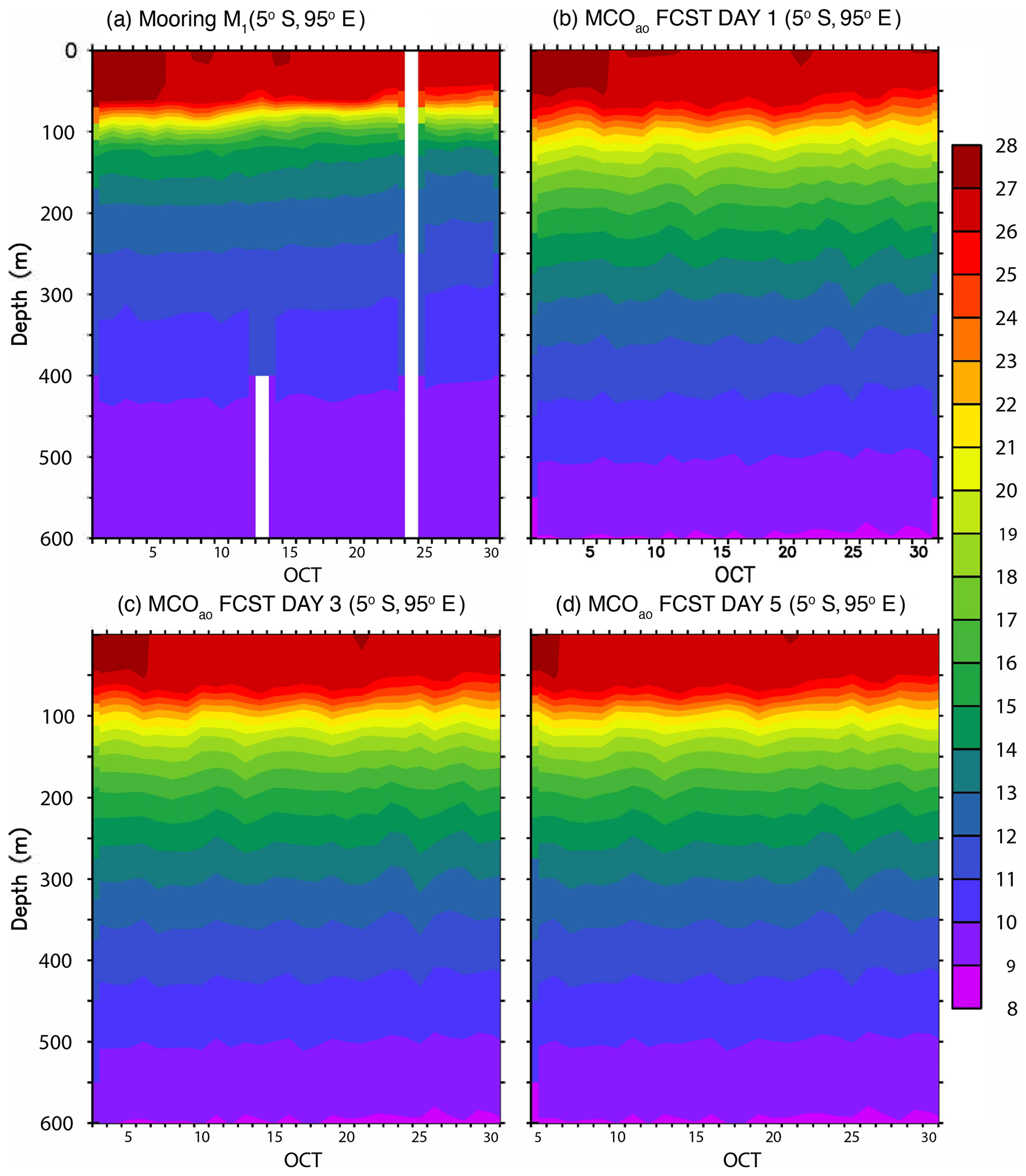
Figure 9 Depth–time plots of temperature (^∘C) at the M₁ mooring location from (a) buoy observations and model forecast (b) fcst_day1, (c) fcst_day3, and (d) fcst_day5. The x axis starting date is different between (c) and (d).

Argo and XBT profiles available for the period 1 October to 5 November 2019 are compared with the model forecast to derive the RMSD statistics for temperature and salinity. Since no temperature or salinity profiles are available in the SCS (figure not shown, data distribution can be viewed from http://www.coriolis.eu.org/Data-Products/Data-Delivery/Data-selection, last access: 6 November 2020), the analysis mainly demonstrates the model performance in the domain excluding the SCS region. As observed in the M₁ mooring location, warm biases with varying magnitude are seen in the thermocline region across the analysis domain (figures not shown). Considering the depth range where this bias exists, the vertical mixing parameterisation may have a stronger influence in modifying the thermal stratification than the penetrative shortwave forcing. Statistics of RMSD for ocean temperature and salinity relative to all profile observations are given in Table 6. RMSD of individual profiles are first computed and then a root-mean-square (rms) value of the computed RMSD is derived. RMSD across all forecast lead times and with the number of profiles analysed are listed. For both temperature and salinity, the RMSD remains fairly similar during the entire analysis period. Over the analysis domain and across all forecast lead times, the maximum RMSD for temperature and salinity are 1.41 ^∘C and 0.14 psu, respectively. Overall, the model forecast deviation relative to the observations is within acceptable error limits of operational forecast models (e.g. Zhang et al., 2010; Yang et al., 2016).

4.2.3 Sea surface height

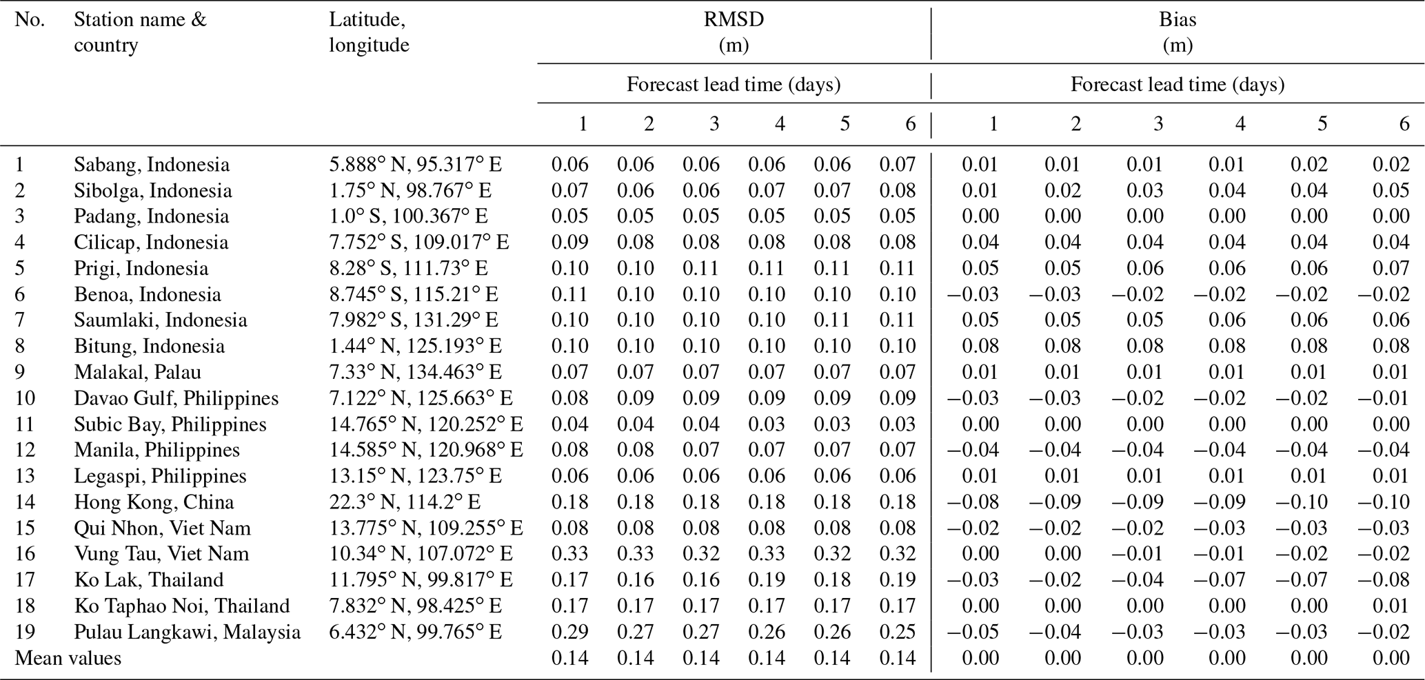
The same set of tide gauge stations used for the MCO hindcast validation has been employed for MCO_ao SSH forecast evaluation. Due to irregularities in the time series, the Currimao Ilocos Norte station is not included in the analysis. Hourly instantaneous SSH data from the model forecast and tide gauge observations are used for the statistical analysis. A summary of SSH RMSD and bias statistics relative to the observations is listed in Table 7. Time series of hourly instantaneous SSH at randomly selected tide gauge stations (Sibolga, Prigi and Vung Tau) and the MCO_ao forecast (fcst_day1) are plotted in Fig. 10. Model SSH bias is within ±0.10 m at all tide gauge stations and forecast lead times. The SSH bias is within ±0.05 m for 14 of total 19 tide gauge stations across all forecast lead times. Since the tide gauges are mostly located near to the coast, SSH variability shorter than intra-seasonal timescale may be largely driven by the tidal forcing. Eventually, in the SSH bias there will be an offset between high and low tidal peaks. Hence, RMSD will give a better representation of model accuracy in tide-dominated regions. RMSD above 0.15 m is observed at the tide gauge stations in Hong Kong (0.18 m), Vung Tau (0.33 m), Ko Lak (0.19 m), Ko Taphao Noi (0.17 m), and Pulau Langkawi (0.29 m). The SDs of SSH observations at these stations during October 2019 are 0.46, 0.82, 0.40, 0.71, and 0.73 m, respectively, and the model forecast error is low relative to the observed SD. No significant variation in model forecast accuracy or RMSD is seen with the increase in forecast lead time. The SSH RMSD is less than 0.10 m for 13 of the total 19 tide gauge stations across all forecast lead times. Overall, the model-simulated SSH shows good agreement with the observations.

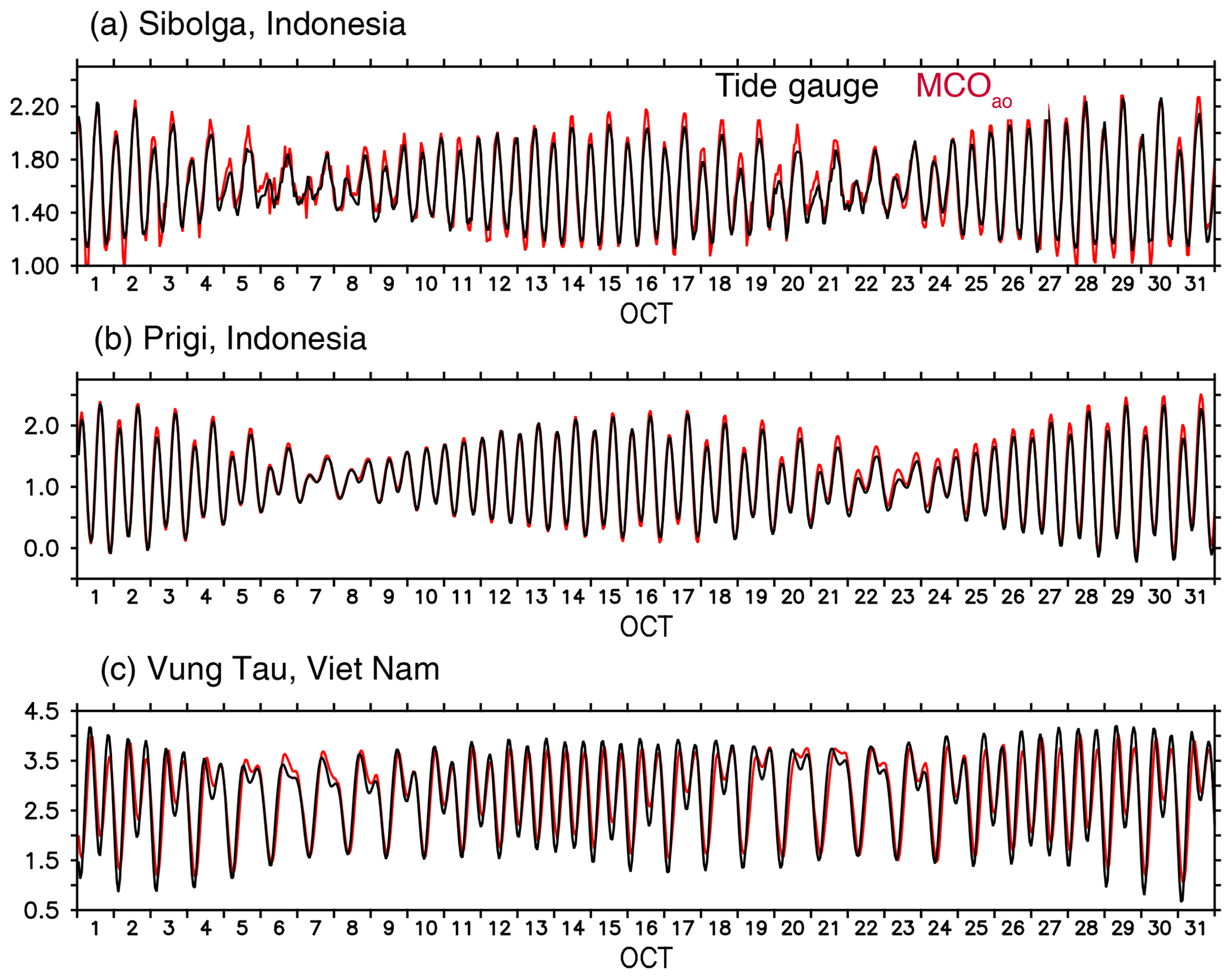
Figure 10 Time series of hourly instantaneous SSH (in metres) from tide gauge observations (black line) and a MCO_ao forecast lead time of 1 d (fcst_day1, red line) at randomly selected stations, (a) Sibolga (1.75^∘ N, 98.767^∘ E), (b) Prigi (8.28^∘ S, 111.73^∘ E), and (c) Vung Tau (10.34^∘ N, 107.072^∘ E), during October 2019.

5 Summary and future developments

The Maritime Continent has a profound influence on the global climate system because of its complex topography and unique geographic location within the tropical Indo-Pacific warm pool. The MC region is characterised by strong atmosphere–ocean coupled processes across multiple timescales. A coupled convective-scale, eddy-resolving atmosphere–ocean modelling system for the western MC, described in T18, was able to improve the simulation of a cold-surge event, the intensity of Typhoon Sarika, and its atmosphere–ocean interactions. Several upgrades have been added to the T18 model for a future operational implementation, such as extending the eastern boundary of the model domain to the western Pacific Ocean, improved science configuration of the atmospheric model (MetUM), and incorporation of tidal boundary forcing to the ocean model (NEMO). Furthermore, the coupled model's feasibility for use as an operational forecast system is also being tested. Typical runtimes of the daily forecast simulations in our experiments are found to be suitable for the operational forecast applications.

The MC_ao coupled prediction system was run as a pre-operational forecast system from 1 to 31 October 2019. Hindcast simulations performed for the period 1 January 2014 to 30 September 2019, using the uncoupled ocean model MCO, provided the initial condition to the MCO_ao. This paper presents details of an atmosphere–ocean coupled prediction system developed for the MC and evaluations of ocean-only model hindcasts and 6 d ocean forecast simulations performed using the coupled system.

The evaluation of MCO hindcast is intended to understand the model's performance in reproducing the past ocean variability, particularly at the ocean surface where the exchange of fluxes between the atmosphere and ocean takes place. The ERA5-driven simulations during the period from 1 January 2018 to 30 June 2019 are utilised for the evaluation of MCO. The SST RMSD between the model hindcast and OSTIA is less than 0.5 ^∘C for about 97 % of the analysis domain. Their correlation is above the 99.9 % confidence level, with about 88 % of the analysis domain displaying correlation higher than 0.8. An SST cold bias is seen in the Andaman Sea, while most of the South China Sea, equatorial western Pacific Ocean, and Australian coast of the Timor Sea show a warm bias. Overall, the mean SST bias, RMSD, and mean correlation over the domain are 0.07 ^∘C, 0.34 ^∘C, and 0.90, respectively.

Comparison of model SST with the RAMA moored buoy observations located at the southeastern tropical Indian Ocean shows good agreement. The SST bias, RMSD, and correlation coefficient between the model and observation are 0.17 ^∘C, 0.29 ^∘C, and 0.94, respectively, for M₁ and 0.12 ^∘C, 0.41 ^∘C, and 0.92, respectively, for M₂ locations. The SSH RMSD is less than 0.10 m for 18 of total 20 tide gauge stations analysed, and 14 stations show RMSD less than 0.05 m. Comparison of model-simulated SST and SSH fields show good agreement with observation and analysis data. Statistically significant correlation with observation suggests that both the spatial and temporal patterns of variability are reasonably well reproduced by the model.

For the evaluation of MCO_ao, comparisons of ocean forecast for different forecast lead times with OSTIA SST and in situ observations have been performed. The forecasted SST over most of the sub-regions is within the error standard deviation of the OSTIA. Though the model forecast exhibits a warm SST bias, the RMSD is less than 0.45 ^∘C over most of the sub-regions during the analysis period. Generally, the forecasted SST tends to be cooler with an increase in forecast lead time, denoting a lower warm bias and RMSD relative to fcst_day1. Overall, the SST correlation over the analysis domain is above the 99 % confidence level across all forecast lead times, while the bias and RMSD are less than 0.19 and 0.35 ^∘C, respectively.

The diurnal variability of SST at the RAMA moored buoy locations M₁ and M₂ are reasonably well reproduced by the model across all forecast lead times. SST bias and RMSD at M₁ are less than 0.0 and 0.20 ^∘C, respectively, and remains fairly constant across all forecast lead times. Meanwhile, the RMSD at M₂ is relatively low, with a maximum of 0.18 ^∘C across all forecast lead times. The depth of the upper ocean isothermal and mixed layer at the M₁ is well forecasted by the model. To understand the model skill in predicting subsurface temperature and salinity, in situ profile observations are compared with the model forecast for different forecast lead times. For both temperature and salinity, the RMSD remains fairly constant during the entire analysis period.

Comparison of model-forecasted SSH shows good agreement with the tide gauge observations. About 75 % of the stations show bias within ±0.05 m at all forecast lead times. No significant variation in model forecast accuracy or RMSD is seen with the increase in forecast lead time. About 73 % of total stations show RMSD less than 0.10 m for all forecast lead times. Overall, the model forecast deviation of SST, SSH, and subsurface temperature and salinity fields relative to observation is within acceptable error limits of operational forecast models (e.g. Zhang et al., 2010; Yang et al., 2016).

Analysis of subsurface fields revealed that significant model temperature biases exist in the region below the mixed layer. The representation of stratification in the thermocline region is relatively weak in the model forecast than the observations. This subsurface temperature bias remains across the model domain with varying magnitudes. Similar temperature biases were reported earlier in simulations with identical model configurations (e.g. Graham et al., 2018). Further modelling work is needed to improve the thermal stratification through fine-tuning the mixing coefficients or modifying the vertical mixing parameterisation.

Further analysis of model forecast fields using longer forecast simulations with increased observations will be undertaken to assess the model predictability across different seasons and during typical weather events such as a cold surge, a typhoon, or the MJO. In addition, the impact of coupling on the forecast will be investigated by performing simultaneous stand-alone ocean model forecast simulations. In addition, work is ongoing to improve our understanding of the forecast skill of MCA_ao, and results from that analysis will be presented as research publications (Kumar et al., 2021). The analysis of model-forecasted precipitation, surface wind, pressure, relative humidity, etc., will be undertaken. The comparisons of coupled and atmosphere-only forecasts will also be performed in that study.

The evaluation of sea surface salinity and ocean current fields is not included in the present study mainly due to the lack of in situ and satellite observations. The South China Sea remains as an especially data-sparse region in terms of the subsurface observations, which highlights the necessity of coordinated efforts from the scientific community to fill these spatial data gaps.

In our analyses, the RMSD and positive or negative biases of the ocean forecasts are generally comparable to those observed from the hindcast statistics. This suggests that, up to a certain extent, the model forecast deviation is inherited from the MCO hindcast or the MCO_ao initial condition. The dependency of model forecast quality on the initial state is well established in the numerical weather prediction studies. Over the tropical oceans specifically, the initialisation of the ocean state is an important element of the forecast systems. The data assimilation techniques help to acquire an improved estimate of the ocean state by combining the model-simulated fields and observations (King et al., 2018). Both the uncoupled and coupled ocean configurations used in our study are free-running models with no restoring or relaxation to the real world. Hence, to provide a better initial condition to MCO_ao, implementation of data assimilation capability for MCO will be a key priority in our future developments. In addition, earlier studies have shown that including wave-induced mixing in ocean circulation model yields a better representation of the upper-ocean temperature (Lewis et al., 2019b). Thus, work towards the development of a three-way atmosphere–ocean–wave coupled system will be undertaken in the future.