the Creative Commons Attribution 4.0 License.
the Creative Commons Attribution 4.0 License.
 | 21 Feb 2020
An evaluation of clouds and radiation in a large-scale atmospheric model using a cloud vertical structure classification
Dongmin Lee
Lazaros Oreopoulos
Nayeong Cho
We revisit the concept of the cloud vertical structure (CVS) classes we have previously employed to classify the planet's cloudiness (Oreopoulos et al., 2017). The CVS classification reflects simple combinations of simultaneous cloud occurrence in the three standard layers traditionally used to separate low, middle, and high clouds and was applied to a dataset derived from active lidar and cloud radar observations. This classification is now introduced in an atmospheric global climate model, specifically a version of NASA's GEOS-5, in order to evaluate the realism of its cloudiness and of the radiative effects associated with the various CVS classes. Such classes can be defined in GEOS-5 thanks to a subcolumn cloud generator paired with the model's radiative transfer algorithm, and their associated radiative effects can be evaluated against observations. We find that the model produces 50 % more clear skies than observations in relative terms and produces isolated high clouds that are slightly less frequent than in observations, but optically thicker, yielding excessive planetary and surface cooling. Low clouds are also brighter than in observations, but underestimates of the frequency of occurrence (by ∼20 % in relative terms) help restore radiative agreement with observations. Overall the model better reproduces the longwave radiative effects of the various CVS classes because cloud vertical location is substantially constrained in the CVS framework.
- Article
(1983 KB) - Full-text XML
- BibTeX
- EndNote


The large impact of clouds on the Earth's radiation budget and the growing wealth of satellite-based cloud observations are strong motivators for their systematic assessment in climate models. Such evaluation exercises focus on either cloud properties, the metrics of cloud radiative impact, or ideally on both (Pincus et al., 2008; Nam et al., 2012; Klein et al., 2013; Wang and Su, 2013; Dolinar et al., 2015).
Assessments of cloud properties with satellite observations are not always straightforward for a variety of reasons such as inability to define in the model a particular satellite-observed property or limitations in the satellite observations. For example, the vertically integrated cloud optical depth of the cloudy portion of a model grid cell is an ill-defined quantity that cannot be obtained trivially from the model's optical depth profile since it is intimately associated with a cloud fraction profile, thus making layer optical depths relevant for only the cloudy portions of the grid cell that vary by model height and can conceptually be vertically aligned in various ways. In contrast, vertically integrated cloud optical depth is quite robustly defined in observations since it is measured with passive imagers at a much higher resolution for which overcast conditions can be more safely assumed. Issues such as these have led to the development of “satellite simulators” that transform global climate model (GCM) cloud fields to forms that are closer analogs to their counterparts observed by satellites (e.g., the COSP simulator; Bodas-Salcedo et al., 2011).
The quality of simulated clouds in GCMs can also be measured in terms of the realism of their radiative impact using quantities such as the cloud radiative effect (CRE), i.e., the difference between all-sky and clear-sky fluxes at the spatial scales of a model grid cell (Wang and Su, 2013). This type of comparison can be performed at a variety of spatiotemporal scales and is often quite illuminating, but the interpretation of findings can suffer from inconsistencies in how the estimates are obtained for satellites and models.
This paper is yet another attempt to evaluate clouds in an atmospheric GCM (AGCM), specifically a version of the Goddard Earth Observing System version 5 (GEOS-5) model (Rienecker et al., 2008; Molod et al., 2012), a multipurpose global model that is used for a variety of applications. Both approaches of cloud assessment are used, namely comparison of the cloud fields themselves but also comparison of cloud radiative impacts. Our cloud property evaluation focuses on a single aspect of cloudiness: cloud vertical structure (CVS). The comparison is possible because of recent progress in two areas: active cloud remote sensing, which makes resolving cloud vertical profiles possible, and the development of schemes (subcolumn generators) that create subgrid cloud vertical structures in GCMs. Being able to categorize clouds in terms of a few CVS categories facilitates the comparison between observations and models and enables a more rigorous CRE comparison that evaluates the model's skill with regard to how it simulates the radiative impact of individual CVS classes.
The observational reference dataset of CVS class occurrence and associated radiative fluxes is essentially the same as Oreopoulos et al. (2017), hereafter O17, and spans 4 years (2007–2010). A schematic illustration of the original CVS classes of O17 is reproduced here as Fig. 1. The details of how cloud layer boundaries available in the 2B-CLDCLASS-LIDAR R04 dataset (Sassen and Wang, 2012; see also http://tinyurl.com/2b-cldclass-lidar, last access: 19 February 2020), a joint product coming from CloudSat and CALIPSO (hereafter CC) active cloud radar and lidar observations, were interpreted as cloud layer profiles belonging to one of these classes are described exhaustively in the appendix of O17. The definition of the CVS classes hinges on defining broad categories of high (H), middle (M), and low (L) clouds that are confined to three standard atmospheric layers: one above 440 hPa, another between 680 and 440 hPa, and yet another below 680 hPa, respectively. The vertical level boundaries defining these standard layers come from the International Satellite Cloud Climatology Project (ISCCP), (Rossow and Schiffer, 1991). The reference radiative fluxes come from the 2B-FLXHR-LIDAR R04 CC product (L'Ecuyer et al., 2008; Henderson et al., 2013; Matus and L'Ecuyer, 2017) and are obtained from a radiative transfer algorithm operating on observed and reanalysis output that has at its core retrieved CC cloud properties.
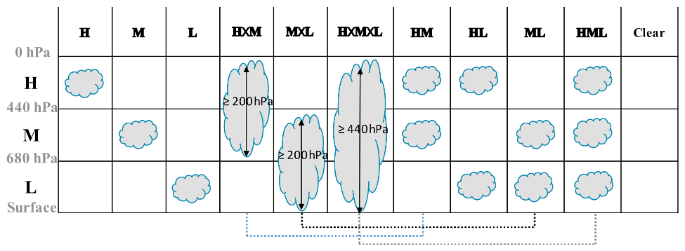
Figure 1The original 10 CVS classes of Oreopoulos et al. (2017) used as a reference for the comparison of this paper. The multilayer CVS classes other than HL are merged in this paper, thus reducing the total number of CVS classes to seven. We essentially do no distinguish between contiguous and noncontiguous clouds in adjacent standard layers. Dotted lines show which pairs of CVS classes have been combined for this study.
For the purposes of this study, the CVS classes have been reduced to seven by merging the CVS classes for which clouds occur simultaneously in the same two or three standard adjacent layers (all multilayer CVS classes other than HL). In other words, we no longer distinguish between CVS classes with clouds occurring in the same adjacent standard layers, even if those were previously discerned based on whether or not a clear layer of substantial vertical extent was present to separate the cloud layers. This means in practice that we no longer distinguish (see Fig. 1) between CVS = and HML (now simply HML), CVS = H×M and HM (now simply HM), or CVS = M×L and ML (now simply ML). The reason for reducing the CVS classes to 7 from the original 10 is the complexity of the model cloud profiles, which can consist of numerous distinct cloud layers and which therefore renders the O17 CVS classification scheme inapplicable. The original scheme was designed for observed cloud profiles from CC that rarely (less than 1 % of the time) consisted of more than four distinct cloud layers in which case they were either ignored or processed only in the simplest of cases (such as multiple individual cloud layers residing within a single standard layer – see the appendix of O17).
A prerequisite for the evaluation of GEOS-5 clouds in terms of their CVS class frequency and the CRE statistics associated with these CVS classes is creating comparable datasets. Assigning CVS classes to grid cell GCM cloud fields is not possible without the manipulation of the GCM cloud profiles. To this end, we use the cloud subcolumn generator that is paired with the RRTMG-LW and RRTMG-SW radiative transfer codes (Mlawer et al., 1997; Iacono et al., 2008) in the model's Monte Carlo independent column approximation (McICA; Pincus et al., 2003) implementation. This subcolumn generator follows Räisänen et al. (2004) and can produce subcolumns that are consistent with specific assumptions about the vertical overlap of both cloud fraction and the horizontal distributions of cloud condensate. While the latter type of overlap is irrelevant to CVS class frequency statistics, it does matter for the radiative transfer calculations producing the radiative fluxes used to estimate CREs. The 140 subcolumns created by the model's generator (which match the number of “g points” in RRTMG-LW's correlated-k scheme) are essentially assumed equivalent to the cloud profiles viewed by the active instruments (CALIPSO's lidar and CloudSat's radar) and whose vertical location information is recorded in the 2B-CLDLASS-LIDAR product. Herein, we will show results from two types of cloud fraction overlap schemes that have been implemented in the cloud subcolumn generator: generalized (GN) overlap, also known as exponential overlap (Hogan and Illingworth, 2000; Oreopoulos and Norris, 2011), and maximum random overlap (MR overlap; Geleyn and Hollingsworth, 1979).
The model, GEOS-5 tag Jason-2_0, was run with fixed sea surface temperatures (SSTs) for the same period as the reference dataset, 2007–2010. The model integration was driven by radiative fluxes and heating rates produced by applying generalized overlap in the radiation calculation. RRTMG-LW and RRTMG-SW were called for an additional set of flux calculations this time using the MR overlap assumption to produce cloudy subcolumns but only in diagnostic mode; i.e., the generated fluxes served only diagnostic purposes and were not passed back to the model to influence the evolution of its energetics and dynamics. This way, with one interactive and one diagnostic call to the RRTMG codes, we were able to obtain two sets of CVS diagnostics and corresponding CREs. In both cases, the subcolumns come from a common mean cloud fraction and condensate profile. The layer condensates are assumed to possess horizontal subgrid condensate heterogeneity as prescribed in Oreopoulos et al. (2012). This subgrid condensate variability affects the model's CRE distribution, but not the CVS fields and statistics.
In the subcolumn generator, the decorrelation length (e-folding distance) for the generalized overlap scheme was set to vary zonally as described in Oreopoulos et al. (2012). The physical meaning of the decorrelation length is that cloud layers separated by a distance equal to the decorrelation length overlap as a mixture of maximum and random overlap in e−1 (≈0.368) and 1-e−1 (≈0.632) proportions (weights), respectively. At distances greater (smaller) than the decorrelation length the contribution of random (maximum) overlap contribution increases (decreases) compared to the above values. In the limit of zero separation cloud overlap is purely maximum, while in the limit of infinite distance overlap is purely random. The zonal prescription of decorrelation length by Oreopoulos et al. (2012) is based on CloudSat observations and is meant to capture a more coherent vertical cloud alignment (i.e., more maximum overlap and greater decorrelation length) at low latitudes compared to high latitudes, as also seen by Barker (2008). This formulation of overlap is an alternative to maximum random overlap, which was the standard popular choice in earlier years. The Geleyn and Hollingsworth (1979) implementation of MR overlap in our generator based on Räisänen et al. (2004) allows for random overlap even within a “block” of contiguous clouds: immediately adjacent clouds are maximally overlapped, but nonadjacent clouds within the contiguous block can have portions that are randomly overlapped if there is a local minimum in cloud fraction between them. Random overlap applies for those cloudy portions that do not fully overlap the in-between layers. This type of MR overlap should be contrasted with other implementations (e.g., Chou et al., 1998) in which maximum overlap always takes place within the block, while the various distinct blocks of the atmospheric column (always separated by clear layers) are themselves randomly overlapped.
3.1 Climatological CVS occurrence
Figure 2 compares the observed and simulated (from GN overlap) multiannual maps of the relative frequency of occurrence (RFO) for all seven CVS classes of our study. The observed fields are sampled at rather coarse scales to compensate for the substantial sparseness of the active observations (gridding at higher resolutions would make for relatively noisy maps). Above each panel, we provide the area-weighted RFO global mean of the CVS (equivalent to its global cloud fraction). These fields include nighttime observations and simulations since the former are possible for active sensors and the latter are passed as input for the model's nighttime RRTMG-LW calculations.
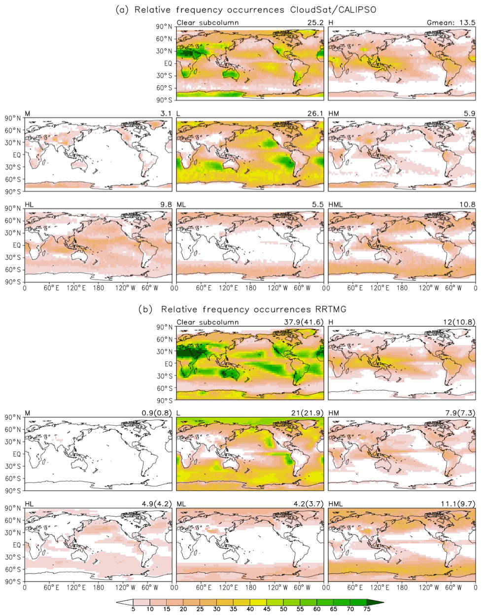
Figure 2Geographical RFO distribution (%) for cloudless skies and the seven CVS classes according to CloudSat/CALIPSO observations (a) as well as for GEOS-5 (GN overlap assumption, b). Global mean values are shown above each panel; in the case of GEOS-5 we provide the global values for both the GN and MR overlap (in parentheses).
Before examining consistency (or lack thereof) for cloud fields, we first turn our attention to clear skies. We note that the observations suggest a cloudier world with clear skies occurring only ∼25 % of the time (or, alternatively, covering 25 % of the global area between 82∘ S and 82∘ N). The GEOS-5 AGCM, on the other hand, produces clear skies more frequently, ∼38 % of the time over the entire globe (90∘ S to 90∘ N) for GN and ∼42 % for MR. Despite the model's positive clear-sky fraction bias (negative cloud fraction bias), many patterns of clear-sky occurrence are realistic, with peaks occurring in desert areas, western North America, and the southern parts of Africa and South America. Over the ocean, the model seems to be producing clear skies in the Maritime Continent and the far southern oceans more frequently than observations, but these overestimates are still much smaller compared to those in wide subtropical swaths of the Atlantic and Pacific oceans. The model also exhibits pronounced cloudiness underestimates in the descending branch of the central Pacific Walker circulation. The only notable model underestimate of clear-sky frequency occurs over western Antarctica. The MR overlap assumption makes the clear-sky overestimates worse, with the biggest impact seen in the central and western tropical Pacific (clear subcolumn in Fig. 3). Note that the observed global clear-sky fraction is lower in 2B-CLDCLASS-LIDAR compared to passive satellite observations such as those from MODIS (King et al., 2003) because of CALIOP's enhanced ability to detect clouds that are optically very thin. Model cloud coverage, on the other hand, has traditionally been tuned to resemble that seen in cloud climatologies obtained by satellite observations from passive imagers at solar and thermal infrared wavelengths.

Figure 3RFO difference (%) maps for clear skies (divided by two to use a common color scale) and the seven CVS classes as simulated by GEOS-5 using the GN and MR overlap assumptions in the cloudy subcolumn generator.
Moving on to cloudy skies, a quick survey of the remaining panels in Fig. 2 reveals that the model exhibits considerable skill in simulating cloudiness when viewed under the prism of CVS classes. Weaknesses, however, become apparent upon closer examination. In terms of global values, the only CVS class in which the model produces a substantial RFO overestimate is HM for both overlap assumptions. For CVS = HML, global RFOs agree, especially for the GN overlap assumption. The global RFOs of all other CVS classes are underestimated to varying degrees, with the underestimates being slightly worse for the MR overlap assumption, except for CVS = L for which MR RFO slightly exceeds GN RFO. The total RFO of the four CVS classes containing H clouds is ∼40 % in observations and ∼36 % (GN) or ∼32 % (MR) in the model. The remaining CVS classes consisting of only L and M clouds add up to a global RFO of ∼35 % in observations and ∼26 % in the model (both GN and MR). Therefore, most of the 13 % discrepancy between GEOS-5 and GN in global cloud fraction comes from the three CVS classes containing only L and M clouds, while the larger discrepancy of ∼17 % for GEOS-5 and MR is more evenly split between these three CVS classes and the remaining four containing H clouds.
A closer comparison of geographical features is also informative. Figure 2b shows only the GN overlap results and can be directly compared with Fig. 2a showing the observed maps. The performance of the MR overlap implementation can be gleaned in terms of its deviation from GN in the Fig. 3 difference maps.
Simulating low clouds has been identified as a challenge for large-scale models, but this version of GEOS-5 seems to be simulating the isolated low clouds (CVS = L) quite well, with a global underestimate of ∼5 % for GN overlap and ∼4 % for MR (absolute values), as well as with characteristic cloud patterns associated with marine stratocumulus being present albeit with less extensive spatial coverage. While GEOS-5 does not produce isolated M clouds (CVS class M) as often as in the observations, the impact is expected to be small as this CVS class is the least frequently observed exclusively over land, specifically deserts, ice- and/or snow-covered surfaces, and regions of pronounced orography. Overall, however, there is not such a great paucity of M clouds in the model when taking into account the other CVS classes containing this type of cloud. Setting aside deep and multilayer clouds (the HML CVS class), M clouds appear only about 11 % (for GN – the figure rises to 22 % for MR) more frequently (in relative terms) in observations than the model; the combined RFO of M, ML, and HM is 14.5 % in the observations and 13 % (11.8 %) in the model for the GN (MR) implementation. Finally, H over L clouds (CVS class HL) are one of the biggest contributors to the overall cloudiness discrepancy between the real and simulated worlds as they appear twice as often in the observations as in the GN version of the model (and even more relative to the MR implementation of the model). The model seems to be lacking much of the tropical presence of this CVS class.
A closer look at the influence of the overlap assumption on CVS RFOs can be gauged from the Fig. 3 maps. We have previously seen that the MR overlap assumption generally produces less cloudiness than GN. This happens systematically (i.e., virtually all locations) for five out of seven CVS classes. The interesting exception is CVS = L (CVS = M is absent in GEOS-5 for all practical purposes). The Fig. 3 difference map for CVS = L reveals that the GN's reduced cloudiness comes mostly from the extratropics; tropical and subtropical pockets can be found where the GN cloud amounts exceed those from MR, as in the other CVS classes. The contrast between CVS = L and the other CVS classes illustrates the fact that the specific flavors of these overlap assumptions as implemented in GEOS-5 can produce a variety of outcomes that depend on the total geometrical extent of contiguous or noncontiguous vertical cloud configurations and the detailed shape of the cloud fraction profile.
3.2 Global CRE comparison by CVS class
Figure 4 compares the global mean CRE between the model and observations, the latter () coming from the aforementioned 2B-FLXHR-LIDAR CC product. It shows the mean values only when the CVS occurs; i.e., CRE is weighted by area, but not by global RFO. We call this type of CRE the “cloudy column” or “overcast” CRE since it is calculated by taking the mean of the CRE values of cloudy subcolumns belonging to the CVS class. CRE values for each cloudy subcolumn also correspond to overcast conditions since there is no partial cloudiness at the subcolumn scale. We show overcast CRE from three perspectives: the top of the atmosphere – TOA (Fig. 4a), the surface – SFC (Fig. 4c), and the atmospheric column – ATM (Fig. 4b), the latter derived as the difference between the TOA and SFC CREs. Moreover, we distinguish between shortwave (SW) and longwave (LW) components and also display their sum, which we call “total” CRE (also called “net” CRE). With CRE being defined as the difference between cloudy and clear-sky net (down–up) fluxes, negative values indicate a radiative cooling effect, while positive values indicate a radiative warming effect. For TOA and SFC, all SW CREs are negative. Note also the magnitudes at TOA and SFC being rather similar for SW, with the slightly larger SFC value resulting from the small positive ATM SW CRE, which indicates that clouds slightly enhance atmospheric column absorption. While LW CREs at both TOA and SFC are positive and therefore indicative of warming, the ATM LW CRE can be either positive or negative. Note that all positive global means involve H clouds. Again, we show model results for the two overlap assumptions, GN and MR, although their CREs are quite close in general. The observed SW CREs depend strongly on the incoming solar flux at the approximate 13:30 local overpass time and are therefore scaled to diurnal fluxes by normalizing with the ratio of the instantaneous to diurnally averaged incoming solar flux at TOA (O17); the LW CREs are simple averages of the daytime and nighttime overpass values. On the other hand, both SW and LW CREs from the model are daily averages of 3-hourly mean outputs.
For TOA SW CRE, the best agreement between model and observations occurs for CVS = L and CVS = HM. For the remaining CVS classes the model either overestimates (CVS = H, M, HL) or underestimates (CVS = ML, HML) overcast TOA SW CRE. The overestimate for CVS class H is very large in relative terms given the small absolute magnitude of the observed CRE. It appears then that H clouds in the model are optically thicker than in observations. Discrepancies are smaller for TOA LW CRE, reflecting the lesser dependence of this quantity on cloud properties other than cloud-top location (which is constrained because of the CVS class decomposition) once clouds reach a certain value of optical thickness (∼5). The biggest bias (underestimate) appears for CVS = HML CVS, but since it is still smaller than the SW CRE bias it results in an underestimate of net planetary cooling as expressed by total TOA CRE (purple bars). Given the better agreement between LW CREs, total TOA CRE biases largely follow the sign of the SW CRE biases. These findings are very insensitive to the type of chosen overlap, although the differences in magnitudes between the two simulated values are still large enough to be distinguishable in most cases.
When moving to an examination of surface (SFC) CREs (Fig. 4c) our conclusions about the SW CRE component are the same as before since atmospheric (ATM) SW CREs are small positive values (panel b). LW CRE values are again simulated quite well since most of the variability is driven by the location of the cloud bottom, which is constrained by CVS class. The largest biases occur for CVS = L and HL (overestimates by the model), and since the TOA CREs have small biases for those cases, errors (excessive cooling) materialize in the ATM LW CRE. Still, the largest ATM LW CRE error occurs for CVS = HM (excessive warming by the model) because the TOA and SFC CRE errors are in the opposite direction. Given the small magnitude of ATM SW CRE, the total ATM CRE errors track those of the LW component.
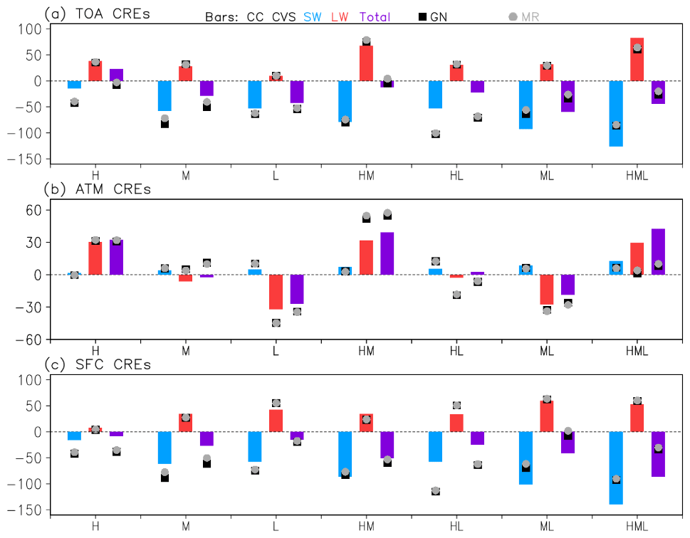
Figure 4Comparison between observations and the model (GN and MR) of global overcast CREs (Wm−2): top of the atmosphere (TOA) (a), surface (SFC) (c), and atmospheric column (ATM) (b) derived as the difference between the TOA and SFC CREs. CREs are distinguished into shortwave (SW) and longwave (LW) components, and their sum, the “total” CREs for each CVS class, are also shown. Note that the y-axis range is the same for TOA and SFC CRE, but it is substantially more compressed for ATM CRE.
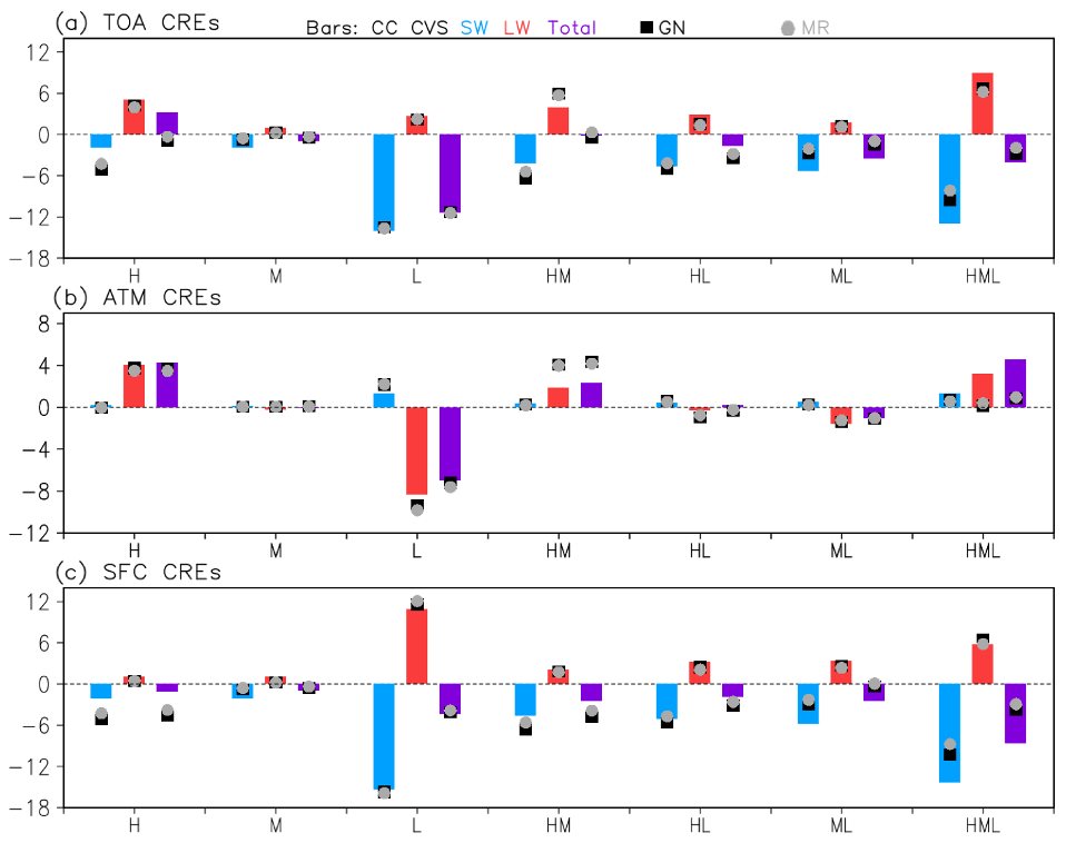
Figure 5 compares observed and modeled CRE values that are now weighted by the global mean RFO ( for observations) of the CVS classes in addition to areal weighting. We can call this type of CRE “all-sky” CRE since in the calculation of the mean all subcolumns that do not belong to the CVS class under consideration contribute zero errors. Summing then these CVS-specific values yields the true global CRE of observed and modeled CRE fields. Since the all-sky CRE values and the range of the y axis are much smaller than in Fig. 4, it makes sense to compare the two figures only with respect to relative biases, essentially focusing on the position of the symbols (simulated values) relative to the bar (observed values). While this will be shown more explicitly in Fig. 6, comparison of Figs. 4 and 5 basically indicates whether RFO errors suppress (i.e., compensate for) or amplify cloud property only errors. Take CVS = HL, for example: RFO errors (underestimates) help suppress the TOA and SFC SW (and total) overestimates. In general, we do not see much of the opposite effect, i.e., an amplification of relative error CRE when moving from overcast to all-sky CRE. Of course, a very low RFO also makes an overcast CRE that previously seemed substantial disappear, with CVS = M being a characteristic case in point. The discussion of all-sky CRE error interpretation continues in the next subsection where a more formal error decomposition framework is introduced.
3.3 CRE error decomposition
Figure 6 shows the decomposition of GEOS-5 all-sky CRE global errors ΔCRE in Fig. 5 to overcast CRE and RFO error contributions for the GN case only (the conclusions remain the same for MR). The decomposition can be expressed as follows (e.g., Tan et al., 2015):
This representation of CRE error arises when the model global all-sky CRE of a CVS class (Fig. 5) is expressed as the product of a deviation Δr from the observed mean overcast CRE (Fig. 4), and the model global RFO is expressed as a deviation Δf from the observed mean RFO, :
Basically, the model's grid-mean CRE error for a CVS class arises from a combination of overcast CRE bias Δr under the observed RFO and the simulated RFO bias Δf under observed overcast CRE , plus a covariation term of RFO and CRE errors under observed and (Tan et al., 2015). Such a decomposition of CRE error allows us to infer, for example, whether the model's poor simulation of all-sky CRE is mostly due to errors in simulating the occurrence frequency of the CVS class or errors in the optical and physical properties of the CVS class that drive the overcast CRE. Similarly, it potentially reveals cases in which good simulations of global all-sky CRE in Fig. 5 benefit from compensating errors in simulated RFO (Fig. 2) and overcast CRE (Fig. 4).
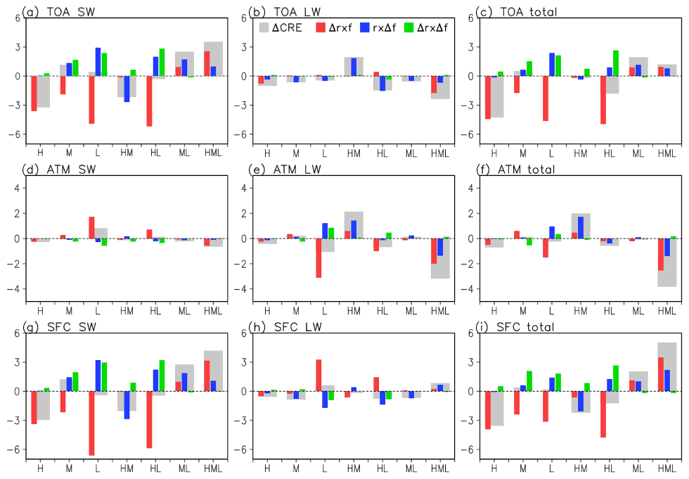
Figure 6Decomposition of all-sky CRE error (Eq. 1) for GEOS-5 CVS classes when the GN overlap assumption is used. Gray bars represent the overall all-sky CRE error, and the remaining bars represent contributions to that error as follows: red bars represent overcast CRE errors, blue bars RFO errors, and green bars covariation errors. The nine panels represent all combinations of CRE, namely SW, LW, total at TOA, SFC, and within ATM.
Separate panels are used in Fig. 6 for SW (a, d, g), LW (b, e, h), and total (c, f, i) CRE. The breakdown by TOA, SFC, and ATM is also preserved, thus yielding a total of nine panels. In the SW, TOA (Fig. 6a), and SFC (Fig. 6g) results look again very similar, while the ATM CRE errors (Fig. 6d) are too small to merit discussion. For most CVS classes (five out of seven) all-sky SW CRE errors (gray bars) come from overcast CRE errors (red bars), namely errors in CVS optical properties. The excessive planetary cooling of the cloudy columns (negative red bars, four CVS classes) is always dampened by compensating errors, sometimes virtually eliminating the error (as in CVS = L, HL), reducing it slightly (CVS = H), or overcorrecting (CVS = M). SW TOA overcast CREs (red bars in Fig. 6a) in the opposite direction (cooling underestimates) become bigger all-sky errors due to RFO errors for CVS = ML and HML, while the all-sky errors for CVS = HM come almost exclusively from RFO errors (blue bars in Fig. 6a). Finally, three CVS classes have sizable covariation errors (green bars) in the same direction as RFO errors. The above error interpretation is virtually the same for surface (SFC) SW errors (Fig. 6g).
Contrary to the SW, the LW CRE errors for all three vantage points (TOA in Fig. 6b, SFC in Fig. 6h, ATM in Fig. 6e) deserve their own discussion as they have different characteristics. At TOA and SFC, the errors are substantially smaller than their SW counterparts. Three of the four CVS classes with H clouds (the exception being CVS = H) exhibit ∼2 Wm−2 (absolute) errors, coming from RFO contributions in two out of the three classes. These three classes have smaller all-sky errors at the SFC, in one case (CVS = HL) because of compensating errors. The largest component errors occur for CVS = L, which has the largest absolute magnitude of all-sky SFC CRE, but with component errors in the opposite direction, compensation reduces the all-sky CRE error. Because the TOA errors for this CVS class are small, the SFC errors carry to the ATM errors. The other CVS class with large ATM error is HML, whereby TOA and SFC errors of the opposite sign conspire to magnify the ATM error.
Errors in total all-sky CRE are driven mainly by SW errors at TOA and SFC (Fig. 6c and i) as well as LW errors for ATM (Fig. 6f). Errors of the opposite sign reduce the overcast cooling error at the SFC for CVS = L and HL and the all-sky warming error for CVS = ML. But because the SFC LW CRE errors are in general small, the total CRE SFC errors largely retain the characteristics of the SW component. In the atmospheric column, SW and LW overcast (and all-sky) errors are additive for CVS = HML and opposing for CVS = L, the only two classes for which ATM SW CRE registers errors of notable magnitude (see Figs. 4b and 5b).
In summary, this decomposition analysis showed the multiple ways relatively good agreement with observed all-sky CRE values from various vantage points can be achieved by GEOS-5 (or any other model evaluated this way). Overcast CRE and RFO errors can compensate, TOA and SFC all-sky CRE errors can compensate (for ATM LW CRE, e.g., CVS is M, ML), SW and LW errors can compensate for total CREs, and finally the errors among various CVS classes can compensate towards decreasing the global CRE error.
3.4 Seasonal CRE comparison
Figures 7–9 compare the multiyear mean annual cycle of TOA, SFC, and ATM total (SW + LW) all-sky CRE zonal averages between observations and the model (employing the GN overlap assumption) for the four CVS classes with the greatest all-sky SW or LW CREs according to Fig. 5.
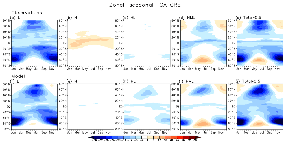
Figure 7Comparison of the multiyear annual cycle of TOA total (SW + LW) all-sky CRE zonal averages (W m−2) between observations (top row, panels a to e) and the model (bottom row, panels f to j) when employing the GN overlap assumption for the four CVS classes with the greatest all-sky CREs according to Fig. 5. The rightmost panels displays the scaled (half) total CRE of all CVS classes combined.
Inspection of the TOA and SFC CRE plots shows that the model has some skill in simulating the seasonal competition between SW and LW CRE, but this should not come as a surprise as it is driven mainly by seasonal changes in insolation. Basically, with everything else staying the same, the SW CRE contribution to total CRE scales with the amount of incoming solar energy. Positive values of total TOA and SFC CRE occur when the solar insolation is weak during the winter, thus allowing the positive LW CRE to exceed the negative SW CRE. At TOA, this takes place only for the HML CVS class since this is the class with competing SW and LW CREs of relatively large magnitude. Note that the model summer planetary cooling is stronger than in the observations. At the SFC, besides CVS = HML the seasonal switch from cooling to warming also takes place for CVS = L because the LW CRE is of comparable magnitude to its SW counterpart. The model's CVS = H is virtually neutral radiatively at TOA throughout the year, in contrast to the observations, for which it provides planetary radiative heating in the tropics and subtropics. It seems then that in the model CVS = H consists of optically thicker clouds that reflect more solar radiation to space than in the real world. H clouds in GEOS-5 also appear to be optically thicker when overlapping with L clouds (CVS = HL), in this case producing planetary cooling in the tropics throughout the year and in the extratropics during the summer months of high insolation, in contrast to the observations for which their cooling effect is very weak and occurs only in the austral extratropics during summertime. Evidence for optically thicker H clouds in both CVS = H and HL is also seen at SFC total CREs, which are more negative in the model than in the observations. Overall (all CVS classes combined; Figs. 7e, j and 8e, j), the model produces a rather realistic pattern of seasonal variations in zonal mean total CRE.

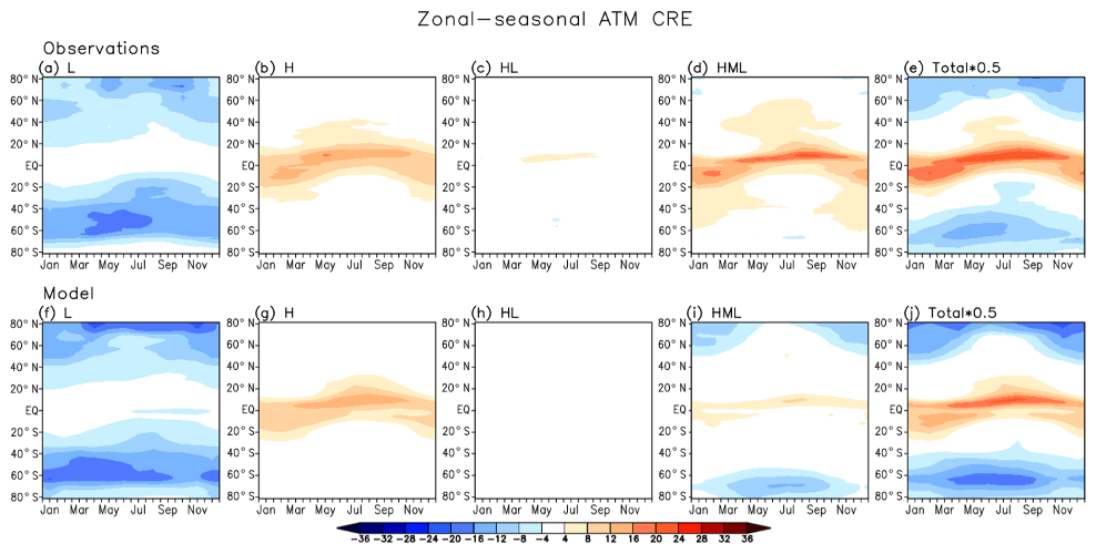
Total ATM CREs are driven, as we have seen earlier, by the LW component, and their seasonal cycles are fairly well represented by the model for three of the four most radiatively important CVS classes (Fig. 9). The nature of CVS = HML, however, seems to be different in GEOS-5 compared to observations. At high latitudes, the atmospheric column is cooled by this type of cloudiness, especially during the summer months, as the SFC total CRE (Fig. 8) exceeds the TOA CRE (Fig. 7). Since the SW contribution is relatively small, it then seems that L clouds within CVS = HML have lower bases or are optically thicker during the summer months in the model compared to observations, making their downward emission towards the surface, and therefore also the contrast between TOA and SFC emission, stronger in the model than the observations. Figure 9i also shows that the near-zero total ATM CRE for CVS = HML in GEOS-5 (Fig. 5) is a result of positive and negative total ATM CRE regional compensations. Overall, the model captures the basic zonal pattern of atmospheric heating and warming (Fig. 9e, j), with heating prevailing in the tropics and cooling in the extratropics. The tropical heating is, however, weaker than in the observations, while the extratropical atmospheric cooling is stronger.
We have introduced a method of cloud evaluation for large-scale atmospheric models that focuses on the vertical structure of cloudiness. Cloud vertical structure (CVS) is resolved in a rather simplified way based on the various combinations of cloud presence in three standard layers that have been traditionally used to distinguish between high, middle, and low clouds. A reference dataset for such CVS classification now exists because of CloudSat and CALIPSO active sensor observations (Oreopoulos et al., 2017). For the purposes of model evaluation, the initial dataset of 10 CVS classes was simplified to consist of 7 classes by merging some of the original classes that had clouds in adjacent standard layers. Beyond comparison of the frequency of occurrence of the CVS classes we also compared their radiative impact in terms of the cloud radiative effect (CRE). While the CVS classes by design constrain cloud vertical location (albeit not in the strictest of ways), they constrain extinction to a lesser extent and mostly qualitatively (e.g., multilayer cloud configurations are expected to have a greater total column extinction). This is taken into account when examining the performance of the model in terms of SW and LW CRE. We developed a framework wherein we can compare CRE for only when a CVS class occurs (overcast CRE) or perform a comparison that also accounts for how frequently the CVS class occurs (all-sky CRE). We can then naturally examine to what extent errors in the latter type of CRE come from errors in the overcast CRE of the class and/or biases in the frequency of occurrence.
The GEOS-5 model under evaluation produces about 50 % more clear skies than observations in relative terms. It produces isolated high clouds (cloud top and base above the 440 hPa level) that are slightly less frequent than in observations but are optically thicker, yielding excessive planetary and surface cooling. Low clouds (cloud tops and bases within the lowest layer of the troposphere up to 680 hPa) are usually a challenge for global models, but GEOS-5 is doing reasonably well and compensates for a lower frequency of occurrence (by ∼20 % in relative terms) with overestimates in extinction, producing in the end an excellent agreement with observations for SW and LW all-sky CREs at either the TOA, SFC, or the atmospheric column vantage points. Overall LW CREs are better simulated since they are mainly driven by vertical cloud location, which is substantially constrained when clouds are broken by CVS class. But either component of CRE can be off in terms of the contribution to the global CRE if the frequency of occurrence is deficient. The other side of the coin is, of course, that incorrect simulation of the frequency of occurrence can compensate for biased cloud optical and physical properties that determine the overcast CRE of the CVS class. Needless to say, CRE biases among different CVS classes can also cancel out to various degrees when global or regional CREs encompassing all clouds represented by the CVS classes are calculated. In such a holistic view, the model appears able, for example, to reproduce the aggregate planetary feature of atmospheric radiative warming in the tropics and cooling in the extratropics driven by cloud configurations dominated by high and low clouds, respectively, albeit with magnitudes that differ from those observed.
The evaluation we conducted requires that the model has the capability to produce cloudy subcolumns, which are then considered equivalent to the atmospheric column profiles seen by the active observations. There is no unique way to go from mean cloud fraction profiles to subcolumns having layer cloud fractions that are either one or zero. We tried two ways to produce subcolumns that assume different cloud fraction overlaps and obtained rather close results. By adopting our framework of cloud evaluation, which, incidentally, should be used in conjunction with other cloud evaluation methodologies (e.g., cloud regimes as in Jin et al., 2017a, b), one can assess whether other large-scale models are more sensitive (i.e., produce a greater diversity of CVS climatologies) to different overlap assumptions applied to the same original mean cloud fraction profiles. What one should always keep in mind, however, is that no matter how good the cloud subcolumn generator is, observed CVS class global frequencies and patterns cannot be reproduced if the model's underlying mean cloud profiles used as input to the generator are deficient.
The GEOS-5 source code is available under the NASA Open-Source Agreement at: http://opensource.gsfc.nasa.gov/projects/GEOS-5/ (last access: 19 February 2020; NASA, 2020).
DL and LO designed the metrics and experiments. DL adapted the model code for the new metric and performed the simulations. NC processed the observational dataset. DL and NC created the graphics and figures. DL and LO authored the text with contributions from NC.
The authors declare that they have no conflict of interest.
Dongmin Lee gratefully acknowledges funding support from NASA's NIP program, while Lazaros Oreopoulos acknowledges support from NASA's CloudSat and CALIPSO Science Team Program. Resources supporting this work were provided by the NASA High-End Computing (HEC) Program through the NASA Center for Climate Simulation (NCCS) at Goddard Space Flight Center. The reference data used for model evaluation (2B-CLDCLASS-LIDAR and 2B-FLXHR-LIDAR) are available from the CloudSat Data Processing Center at: http://www.cloudsat.cira.colostate.edu (last access: 19 February 2020). We thank our colleague Donifan Barahona for helpful discussions about various model tags.
This research has been supported by the National Aeronautics and Space Administration (NASA) (grant no. 80NSSC18K0997).
This paper was edited by Holger Tost and reviewed by two anonymous referees.
Barker, H.: Overlap of fractional cloud for radiation calculations in GCMs: A global analysis using CloudSat and CALIPSO data, J. Geophys. Res., 113, D00A01, https://doi.org/10.1029/2007JD009677, 2008.
Bodas-Salcedo, A., Webb, M., Bony, S., Chepfer, H., Dufresne, J., Klein, S., Zhang, Y., Marchand, R., Haynes, J., Pincus, R., and John, V.: COSP Satellite simulation software for model assessment, B. Am. Meteorol. Soc., 92, 1023–1043, https://doi.org/10.1175/2011BAMS2856.1, 2011.
Chou, M., Suarez, M., Ho, C., Yan, M., and Lee, K.: Parameterizations for cloud overlapping and shortwave single-scattering properties for use in general circulation and cloud ensemble models, J. Climate, 11, 202–214, 1998.
Dolinar, E., Dong, X., Xi, B., Jiang, J., and Su, H.: Evaluation of CMIP5 simulated clouds and TOA radiation budgets using NASA satellite observations, Clim. Dynam., 44, 2229–2247, https://doi.org/10.1007/s00382-014-2158-9, 2015.
Geleyn, J. F. and Hollingsworth, A.: An economical analytical method for the computation of the interaction between scattering and line absorption of radiation, Contrib. Atmos. Phys., 52, 1–16, 1979.
Henderson, D., L'Ecuyer, T., Stephens, G., Partain, P., and Sekiguchi, M.: A Multisensor Perspective on the Radiative Impacts of Clouds and Aerosols, J. Appl. Meteorol. Climatol, 52, 853–871, https://doi.org/10.1175/JAMC-D-12-025.1, 2013.
Hogan, R. and Illingworth, A.: Deriving cloud overlap statistics from radar, Q. J. Roy. Meteorol. Soc., 126, 2903–2909, https://doi.org/10.1002/qj.49712656914, 2000.
Iacono, M., Delamere, J., Mlawer, E., Shephard, M., Clough, S., and Collins, W.: Radiative forcing by long-lived greenhouse gases: Calculations with the AER radiative transfer models J. Geophys. Res., 113, D13103, https://doi.org/10.1029/2008JD009944, 2008.
Jin, D., Oreopoulos, L., and Lee, D.: Regime-based evaluation of cloudiness in CMIP5 models, Clim. Dynam., 48, 89–112, https://doi.org/10.1007/s00382-016-3064-0, 2017a.
Jin, D., Oreopoulos, L., and Lee, D.: Simplified ISCCP cloud regimes for evaluating cloudiness in CMIP5 models, Clim. Dynam., 48, 113–130, https://doi.org/10.1007/s00382-016-3107-6, 2017b.
King, M., Menzel, W., Kaufman, Y., Tanre, D., Gao, B., Platnick, S., Ackerman, S., Remer, L., Pincus, R., and Hubanks, P.: Cloud and aerosol properties, precipitable water, and profiles of temperature and water vapor from MODIS, IEEE Trans. Geosci. Remote Sensing, 41, 442–458, https://doi.org/10.1109/TGRS.2002.808226, 2003.
Klein, S., Zhang, Y., Zelinka, M., Pincus, R., Boyle, J., and Gleckler, P.: Are climate model simulations of clouds improving? An evaluation using the ISCCP simulator, J. Geophys. Res.-Atmos., 118, 1329–1342, https://doi.org/10.1002/jgrd.50141, 2013.
L'Ecuyer, T., Wood, N., Haladay, T., Stephens, G., and Stackhouse, P.: Impact of clouds on atmospheric heating based on the R04 CloudSat fluxes and heating rates data set, J. Geophys. Res.-Atmos., 113, D00A15, https://doi.org/10.1029/2008JD009951, 2008.
Matus, A. and L'Ecuyer, T.: The role of cloud phase in Earth's radiation budget, J. Geophys. Res.-Atmos., 122, 2559–2578, https://doi.org/10.1002/2016JD025951, 2017.
Mlawer, E. J., Taubman, S. J., Brown, P. D., Iacono, M. J., and Clough, S. A.: RRTM, a validated correlated-k model for the longwave, J. Geophys. Res., 102, 16663–16682, 1997.
Molod, A., Takacs, L., Suarez, M. J., Bacmeister, J., Song, I.-S., and Eichmann, A.: GEOS-5 Atmospheric General Circulation Model: mean climate development from MERRA to Fortuna, Tech. Memo, NASA Goddard Space Flight Center, MD, 115 pp., 2012.
Nam, C., Bony, S., Dufresne, J., and Chepfer, H.: The 'too few, too bright' tropical low-cloud problem in CMIP5 models, Geophys. Res. Lett., 39, L21801, https://doi.org/10.1029/2012GL053421, 2012.
NASA: Goddard Space Flight Center, GEOS-5 Modeling Software, available at: https://opensource.gsfc.nasa.gov/projects/GEOS-5/, last access: 19 February 2020.
Oreopoulos, L. and Norris, P. M.: An analysis of cloud overlap at a midlatitude atmospheric observation facility, Atmos. Chem. Phys., 11, 5557–5567, https://doi.org/10.5194/acp-11-5557-2011, 2011.
Oreopoulos, L., Lee, D., Sud, Y. C., and Suarez, M. J.: Radiative impacts of cloud heterogeneity and overlap in an atmospheric General Circulation Model, Atmos. Chem. Phys., 12, 9097–9111, https://doi.org/10.5194/acp-12-9097-2012, 2012.
Oreopoulos, L., Cho, N., and Lee, D.: New insights about cloud vertical structure from CloudSat and CALIPSO observations, J. Geophys. Res.-Atmos., 122, 9280–9300, https://doi.org/10.1002/2017JD026629, 2017.
Pincus, R., Barker, H., and Morcrette, J.: A fast, flexible, approximate technique for computing radiative transfer in inhomogeneous cloud fields, J. Geophys. Res.-Atmos., 108, D134376, https://doi.org/10.1029/2002JD003322, 2003.
Pincus, R., Batstone, C., Hofmann, R., Taylor, K., and Glecker, P.: Evaluating the present-day simulation of clouds, precipitation, and radiation in climate models, J. Geophys. Res.-Atmos., 113, D14209, https://doi.org/10.1029/2007JD009334, 2008.
Räisänen, P., Barker, H., Khairoutdinov, M., Li, J., and Randall, D.: Stochastic generation of subgrid-scale cloudy columns for large-scale models, Q. J. Roy. Meteorol. Soc., 130, 2047–2067, https://doi.org/10.1256/qj.03.99, 2004.
Rienecker, M. M., Suarez, M. J., Todling R., Bacmeister J., Takacs L., Liu H.-C., Gu W., Sienkiewicz M., Koster, R. D., Gelaro, R., Stajner, I., and Nielsen, J. E.: The GEOS-5 Data Assimila- tion System Documentation of Versions 1 5.0.1, 5.1.0, and 5.2.0. NASA/TM–2008–2 104606, Vol. 27, 118 pp., 2008.
Rossow, W. and Schiffer, R.: ISCCP cloud data products, B. Am. Meteorol. Soc., 72, 2–20, https://doi.org/10.1175/1520-0477(1991)072<0002:ICDP>2.0.CO;2, 1991.
Sassen, K. and Wang, Z.: The Clouds of the Middle Troposphere: Composition, Radiative Impact, and Global Distribution, Surv. Geophys., 33, 677–691, https://doi.org/10.1007/s10712-011-9163-x, 2012.
Tan, J., Jakob, C., Rossow, W., and Tselioudis, G.: Increases in tropical rainfall driven by changes in frequency of organized deep convection, Nature, 519, 451–454, https://doi.org/10.1038/nature14339, 2015.
Wang, H. and Su, W.: Evaluating and understanding top of the atmosphere cloud radiative effects in Intergovernmental Panel on Climate Change (IPCC) Fifth Assessment Report (AR5) Coupled Model Intercomparison Project Phase 5 (CMIP5) models using satellite observations, J. Geophys. Res.-Atmos., 118, 683–699, https://doi.org/10.1029/2012JD018619, 2013.