Automated Monte Carlo-based quantification and updating of geological uncertainty with borehole data (AutoBEL v1.0)

Geological uncertainty quantification is critical to subsurface modeling and prediction, such as groundwater, oil or gas, and geothermal resources, and needs to be continuously updated with new data. We provide an automated method for uncertainty quantification and the updating of geological models using borehole data for subsurface developments within a Bayesian framework. Our methodologies are developed with the Bayesian evidential learning protocol for uncertainty quantification. Under such a framework, newly acquired borehole data directly and jointly update geological models (structure, lithology, petrophysics, and fluids), globally and spatially, without time-consuming model rebuilding. To address the above matters, an ensemble of prior geological models is first constructed by Monte Carlo simulation from prior distribution. Once the prior model is tested by means of a falsification process, a sequential direct forecasting is designed to perform the joint uncertainty quantification. The direct forecasting is a statistical learning method that learns from a series of bijective operations to establish “Bayes–linear-Gauss” statistical relationships between model and data variables. Such statistical relationships, once conditioned to actual borehole measurements, allow for fast-computation posterior geological models. The proposed framework is completely automated in an open-source project. We demonstrate its application by applying it to a generic gas reservoir dataset. The posterior results show significant uncertainty reduction in both spatial geological model and gas volume prediction and cannot be falsified by new borehole observations. Furthermore, our automated framework completes the entire uncertainty quantification process efficiently for such large models.

1 Introduction

Uncertainty quantification (UQ) is at the heart of decision making. This is particularly true in subsurface applications such as groundwater, geothermal resources, fossil fuels, CO₂ sequestration, or minerals resources. Uncertainty on the geological structures, rocks, and fluids is due to the lack of access to the subsurface geological medium. For most of the subsurface applications, knowledge of the geological settings is mainly gained through the drilling of well boreholes where geophysical or rock physical measurements are made. For example, several tens to hundreds of boreholes are drilled in geothermal or groundwater appraisals (e.g., Le Borgne et al., 2006; Klepikova et al., 2011; Vogt et al., 2010), while in mineral resources and shale gas, the number of boreholes can even be in the thousands (e.g., Curtis, 2002; Abbott, 2013). From borehole data, geological models are constructed for appraisal and uncertainty quantification, such as estimating water volumes stored in groundwater systems or heat storage in a geothermal system. Realistic geological modeling involves complex procedures (Caumon, 2010, 2018; de la Varga et al., 2019). This is due to the hierarchical nature of geological formations: fluids are contained in a porous medium, the porous medium is defined by various lithologies, and lithological variation is contained in faults and layers (structure). In addition, boreholes are not drilled all at once but throughout the lifetime of managing the Earth's resource.

Representing the unknown subsurface geological reality by a single deterministic model has been commonly done (Beven, 1993; Royse, 2010), mostly by means of a single realization of the structure (layers or faults), rock, and fluid model derived from the borehole data with other supporting geological and geophysical interpretations (e.g., Fischer et al., 2015; Kaufmann and Martin, 2008). However, relying on a single model cannot reflect the inherent geological uncertainty (Neuman, 2003). Recent advances in geostatistics have shown the importance of using multiple model realizations for uncertainty quantification in many geoscience fields, including glaciology (e.g., Cullen et al., 2017), hydrogeology (e.g., Barfod et al., 2018; Zhou et al., 2014), hydrology (e.g., Goovaerts, 2000; Marko et al., 2014), hydrocarbon reservoir modeling (e.g., Caers and Zhang, 2004; Christie et al., 2002; Dutta et al., 2019; Yin et al., 2019), and geothermal (e.g., Rühaak et al., 2015; Vogt et al., 2010). Geostatistical approaches can provide multiple geological models that are conditioned or constrained to borehole data. When new boreholes are drilled, uncertainty needs to be updated. While uncertainty updating in the form of data assimilation is commonly applied to various subsurface applications, it is rarely used for updating newly drilled borehole data, often termed “hard data” in geostatistical literatures (Goovaerts, 1997). Elfeki and Dekking (2007) used a coupled Markov chain (CMC) approach to calibrate a hydrogeological lithology model by conditioning on boreholes in the central Rhine–Meuse delta in the Netherlands, and they then ran a Monte Carlo simulation to reevaluate the hydrogeological uncertainty. A similar approach was also used by Li et al. (2016) to reduce the uncertainty in near-surface geology for the risk assessment of soil slope stability and safety in Western Australia. Jiménez et al. (2016) updated 3-D hydrogeological models by adding new geological features identified from borehole tracer tests. Eidsvik and Ellefmo (2013) and Soltani-Mohammadi et al. (2016) investigated the value of information of additional boreholes for uncertainty reduction in mineral resource evaluations.

The problem of geological uncertainty, due to its interpretative nature and the presence of prior information, is often handled in a Bayesian framework (Scheidt et al., 2018). The key part often lies in the joint quantification of the prior uncertainty on all modeling parameters, whether structural, lithological, petrophysical, or fluid. A common problem is that the observed data may lie outside the defined prior model and hence are falsified. Another major issue is that most of the state-of-the-art uncertainty updating practices deal with each geological model component separately (a silo treatment of each UQ problem). However, the borehole data inform all components jointly, and hence any separate treatment ignores the likely dependency between the model components, possibly returning unrealistic uncertainty quantification. A final concern, more practically, lies around automating any uncertainty updating. Geological modeling often requires significant individual or group expertise and manual intervention to make the model adhere to geological rules, hence often requiring months of work when new data are acquired. There is to date, no method that addresses, with borehole data, the falsification, the joint uncertainty quantification, and the automation problem.

Recently, an uncertainty quantification protocol termed Bayesian evidential learning has been proposed to address decision making under uncertainty, and it has been applied to cases in oil or gas, groundwater contaminant remediation and geothermal energy (Athens and Caers, 2019; Hermans et al., 2018, 2019; Scheidt et al., 2018). It provides explicit standards that need to be reached at each stage of its UQ design with the purpose of decision making, including model falsification, global sensitivity analysis, prior elicitation, and data-science-driven uncertainty reduction under the principle of Bayesianism. Compared to the previous works on Bayesian evidential learning (BEL), model falsification, statistical learning-based uncertainty reduction approaches, and automation are what is of concern in this paper. Also, we will deal with one specific data source: borehole data, through logging or coring, for geological uncertainty quantification. First, we will introduce a scheme to address the model falsification problem involving borehole data by using robust Mahalanobis distance. We will then extend a statistical learning approach termed direct forecasting (Hermans et al., 2016; Satija et al., 2017; Satija and Caers, 2015) to reduce uncertainty of all geological model parameters jointly, using all (new) borehole data simultaneously. To achieve this, we will present a model formulation that involves updating based on the hierarchy typically found in subsurface formation: structures, then lithology, and then property and fluid distribution. Finally, we will show how the proposed framework can be completely automated in an open-source project. With a generalized field case study of uncertainty quantification of gas volume in an offshore reservoir, we will illustrate our approach and emphasize the need for automation, minimizing the need for tuning parameters that require human interpretation.

2 Methodology

2.1 Bayesian evidential learning

2.1.1 Overview

We establish the geological uncertainty quantification framework based on BEL, which is briefly reviewed in this section. BEL is not a method, but a prescriptive and normative data-scientific protocol for designing uncertainty quantification within the context of decision making (Athens and Caers, 2019; Hermans et al., 2018; Scheidt et al., 2018). It integrates four constituents in UQ – data, model, prediction, and decision under the scientific methods and philosophy of Bayesianism. In BEL, the data are used as evidence to infer model or/and prediction hypotheses via “learning” from the prior distribution, whereas decision making is ultimately informed by the model and prediction hypotheses. The BEL protocol consists of six UQ steps: (1) formulating the decision questions and prediction variables; (2) statement of model parametrization and prior uncertainty; (3) Monte Carlo and prior model falsification with data; (4) global sensitivity analysis between data and prediction variables; (5) uncertainty reduction based on statistical learning methods that reflect the principle of Bayesian philosophy; (6) posterior falsification and decision making. Bayesian methods, particularly in the Earth sciences rely on the statement of prior uncertainty. However, such a statement may be inconsistent with data in the sense that the prior cannot predict the data, hence the important falsification step. We next provide important elements of BEL within the problem of this paper: prior model definition, falsification, and inversion by direct forecasting.

2.1.2 Hierarchical model definition

In geological uncertainty quantification, any prior uncertainty statement needs to involve all model components jointly. A geological model m typically consists of four components that are modeled in hierarchical order: structural model χ (e.g., faults, stratigraphic horizons), rock types ζ (which are categorical, e.g., sedimentary or architectural facies), petrophysics model κ (e.g., density, porosity, permeability), and subsurface fluid distribution τ (e.g., water saturation, salinity).

$$\begin{array}{}\text{(1)}& \mathit{m}=\left\{\mathit{\chi },\mathit{\zeta },\mathit{\kappa },\mathit{\tau }\right\}\end{array}$$

The uncertainty model then becomes the following sequential decomposition:

$$\begin{array}{}\text{(2)}& \begin{array}{rl}f\left(\mathit{m}\right)=& f\left(\mathit{\chi },\mathit{\zeta },\mathit{\kappa },\mathit{\tau }\right)=f\left(\mathit{\tau }\mathbf{|}\mathit{\chi },\mathit{\zeta },\mathit{\kappa }\right)f\left(\mathit{\kappa }\mathrm{|}\mathit{\chi },\mathit{\zeta }\right)\\ & f\left(\mathit{\zeta }\mathrm{|}\mathit{\chi }\right)f\left(\mathit{\chi }\right).\end{array}\end{array}$$

In addition, because of the spatial context of all geological formations, we divide the model variables into global and spatial ones. The global variables, such as proportions, depositional system interpretation, or trend, are scalars and not attached to any specific grid locations, whereas the spatial variables are gridded. Here, we term the global variables as m_gl, and the spatial ones as m_sp In this way, the geological model variables are

$$\begin{array}{}\text{(3)}& \mathit{m}=\left\{\left({\mathit{\chi }}_{\mathrm{gl}},{\mathit{\chi }}_{\mathrm{sp}}\right),\left({\mathit{\zeta }}_{\mathrm{gl}},{\mathit{\zeta }}_{\mathrm{sp}}\right),\left({\mathit{\kappa }}_{\mathrm{gl}},{\mathit{\kappa }}_{\mathrm{sp}}\right),\left({\mathit{\tau }}_{\mathrm{gl}},{\mathit{\tau }}_{\mathrm{sp}}\right)\right\}.\end{array}$$

The prior uncertainty f(m) of the global and spatial variables needs to be specified for each model component; this is problem specific and may require a substantial amount of work by considering the existing data (e.g., the system is deltaic) and any prior knowledge about the interpreted systems. Using the prior distribution f(m), we run Monte Carlo to generate a set of L model realizations $\left\{{\mathit{m}}^{\left(\mathrm{1}\right)},{\mathit{m}}^{\left(\mathrm{2}\right)},\mathrm{\dots },{\mathit{m}}^{\left(L\right)}\right\}$. This means instantiating all geological variables $\mathit{\chi },\mathit{\zeta },\mathit{\kappa },\mathit{\tau }$ jointly.

Since borehole data provide information at the locations of drilling, we define the data variables d through an operator G_d.

$$\begin{array}{}\text{(4)}& \mathit{d}={\mathbf{G}}_d\mathit{m}\end{array}$$

G_d is simply a matrix in which each element is either 0 or 1, identifying the locations of boreholes in the model m. In this sense, borehole data are linear data because of the linear forward operator. By applying G_d to prior geological model realizations, we obtained a set of L samples of the borehole data variable.

$$\begin{array}{}\text{(5)}& \mathit{d}=\left\{{\mathit{d}}^{\left(\mathrm{1}\right)},{\mathit{d}}^{\left(\mathrm{2}\right)},\mathrm{\dots },{\mathit{d}}^{\left(L\right)}\right\}\end{array}$$

Note that we term the actual acquired data d_obs.

The prediction variable h, such as storage volume of a groundwater aquifer or the heat storage of a geothermal reservoir, is defined through another operator (linear or nonlinear):

$$\begin{array}{}\text{(6)}& \mathit{h}={\mathbf{G}}_h\left(\mathit{m}\right).\end{array}$$

Applying this function to the prior model realizations we get

$$\begin{array}{}\text{(7)}& \mathit{h}=\left\{{\mathit{h}}^{\left(\mathrm{1}\right)},{\mathit{h}}^{\left(\mathrm{2}\right)},\mathrm{\dots },{\mathit{h}}^{\left(\mathrm{L}\right)}\right\}.\end{array}$$

A common problem in practice is that the statement of the prior may be too narrow (overconfidence) and hence may not in fact predict the observed data. In falsification, we use hypothetic–deductive reasoning to attempt to reject the prior by means of data, namely by stating the null hypothesis: the prior can predict the observation and attempt to reject it. This step does not involve matching models to data; it is only a statistical test. One way of achieving this is using outlier detection as discussed in the next section.

2.1.3 Falsification using multivariate outlier detection

The goal of falsification is to test that the prior model is not wrong. The prior model should be able to predict the data. Our reasoning then is that a prior model is falsified if the observed data d_obs are not within the same population as the samples ${\mathit{d}}^{\left(\mathrm{1}\right)},{\mathit{d}}^{\left(\mathrm{2}\right)},\mathrm{\dots },{\mathit{d}}^{\left(L\right)}$; i.e., d_obs is an outlier. Evidently, the data variable can be high dimensional due to a large number of wells with various types of measurements on structure, facies, petrophysics, and saturation, which calls for multivariate outlier detection. We propose in this paper to use a robust statistical procedure based on Mahalanobis distance to perform the outlier detection. The robust Mahalanobis distance (RMD) for each data variable realization d^(l) or d_obs is calculated as

$$\begin{array}{}\text{(8)}& \begin{array}{rl}\text{RMD}\left({\mathit{d}}^{\left(l\right)}\right)=& \sqrt{{\left({\mathit{d}}^{\left(l\right)}-\mathit{\mu }\right)}^T{\mathbf{\Sigma }}^{-\mathrm{1}}\left({\mathit{d}}^{\left(l\right)}-\mathit{\mu }\right)},\\ & \text{ for }l=\mathrm{1},\mathrm{2},\mathrm{\dots },L\end{array},\end{array}$$

where μ and Σ are the robust estimation of mean and covariance of the data (Hubert and Debruyne, 2010; Rousseeuw and Driessen, 1999). Assuming d distributes as a multivariate Gaussian, the distribution of [RMD(d^(l))]² will be chi-squared ${\mathit{\chi }}_d^{\mathrm{2}}$. We will use the 97.5 percentile of ${\sqrt{\mathit{\chi }}}_d^{\mathrm{2}}$ as the tolerance for the multivariate dimensional points d^(l). If the RMD(d_obs) falls outside the tolerance ($\text{RMD}\left({\mathit{d}}_{\mathrm{obs}}\right)>{\sqrt{\mathit{\chi }}}_{d,\mathrm{97.5}}^{\mathrm{2}})$, the d_obs will be regarded as outliers, which means the prior model has a very small probability of predicting the actual observations; hence it is falsified. It should be noted that the d_obs dealt with in this paper is at model grid resolution. Outlier detection using the Mahalanobis distance has the advantage of providing robust statistical calculations. In addition, diagnostic plots can be used to visualize the result for high-dimensional data. However, it requires the marginal distribution of data to be Gaussian. If the data variables are not Gaussian, other outlier detection approaches such as one-class support vector machine (SVM) (Schölkopf et al., 2001) or isolation forest (Liu et al., 2008) can be used.

2.2 Direct forecasting

2.2.1 Review

If the prior model cannot be falsified, we will use direct forecasting to reduce geological model uncertainty. Direct forecasting (DF) is a prediction-focused data science approach for inverse modeling (Hermans et al., 2016; Satija et al., 2017; Satija and Caers, 2015). The aim is to estimate/learn the conditional distribution f(h|d) between the prediction variable h and data variable d from prior Monte Carlo samples. Then, instead of using traditional inverse methods that require rebuilding models to update prediction, direct forecasting directly calculates the conditional prediction distribution f(h|d_obs) through the statistical learning based on data. The learning strategy of direct forecasting is that, by employing bijective operations, the non-Gaussian problem f(h|d) can be transformed into a linear-Gauss problem of transformed variables $\left({\mathit{h}}^{\ast },{\mathit{d}}^{\ast }\right)$:

$$\begin{array}{}\text{(9)}& \begin{array}{rl}& {\mathit{h}}^{\ast }\sim \exp \left(-{\displaystyle \frac{\mathrm{1}}{\mathrm{2}}}{\left({\mathit{h}}^{\ast }-{\mathit{h}}_{\mathrm{prior}}^{\ast }\right)}^T{\mathbf{C}}_{\mathrm{prior}}^{-\mathrm{1}}\left({\mathit{h}}^{\ast }-{\mathit{h}}_{\mathrm{prior}}^{\ast }\right)\right);\\ & {\mathit{d}}_{\mathrm{obs}}^{\ast };{\mathit{d}}^{\ast }=\mathbf{G}{\mathit{h}}^{\ast }\end{array},\end{array}$$

where G is coefficients that linearly map h^∗ to d^∗. This makes $f({\mathit{h}}^{\ast }\mathrm{|}{\mathit{d}}_{\mathrm{obs}}^{\ast }$) become a “Bayes–linear-Gauss” problem that has an analytical solution:

$$\begin{array}{}\text{(10)}& {\displaystyle }\begin{array}{rl}& E\left[{\mathit{h}}^{\ast }\mathrm{|}{\mathit{d}}_{\mathrm{obs}}^{\ast }\right]={\mathit{h}}_{\mathrm{posterior}}^{\ast }={\mathit{h}}_{\mathrm{prior}}^{\ast }+{\mathbf{C}}_{\mathrm{prior}}{\mathbf{G}}^T\\ & {\left({\mathbf{GC}}_{\mathrm{prior}}{\mathbf{G}}^T\right)}^{-\mathrm{1}}\left({\mathit{d}}_{\mathrm{obs}}^{\ast }-\mathbf{G}{\mathit{h}}_{\mathrm{prior}}^{\ast }\right),\\ & \mathrm{Var}\left[{\mathit{h}}^{\ast }\mathrm{|}{\mathit{d}}_{\mathrm{obs}}^{\ast }\right]={\mathbf{C}}_{\mathrm{posterior}}={\mathbf{C}}_{\mathrm{prior}}-{\mathbf{C}}_{\mathrm{prior}}{\mathbf{G}}^T\\ & {\left({\mathbf{GC}}_{\mathrm{prior}}{\mathbf{G}}^T\right)}^{-\mathrm{1}}{\mathbf{GC}}_{\mathrm{prior}}\end{array}.\end{array}$$

In detail, the specific steps of direct forecasting are

1. Monte Carlo: generate L samples of prior model and run forward function to evaluate data and prediction variables.

2. Orthogonality: PCA (principal component analysis) on data variable d and prediction variable h.

3. Linearization: maximize linear correlation between the orthogonalized data and variables by normal score transform and CCA (canonical component analysis), obtaining transformed ${\mathit{h}}^{\ast },{\mathit{d}}^{\ast }$.

4. Bayes–linear-Gauss: calculate conditional mean and covariance of the transformed prediction variable.

5. Sampling: sample from the posterior distribution of transformed prediction variable ${\mathit{h}}_{\mathrm{posterior}}^{\ast }$.

6. Reconstruction: invert all bijective operations, obtaining h_posterior in the original space.

One key question in direct forecasting is how to determine the Monte Carlo samples size L. Usually, the samples size L lies between 100 and 1000, according to the studies in water resources (Satija and Caers, 2015), hydrogeophysics (Hermans et al., 2016), and hydrocarbon reservoirs (Satija et al., 2017).

Direct forecasting can also be extended to update model variables, by simply replacing the prediction variable h by model variable m in the above algorithms, to obtain f(m|d_obs) without conventional model inversions (Park, 2019). However, the high dimensionality of spatial models (millions of grid cells) imposes challenge to such an extension. This is because CCA requires the sum of input data and model variable dimensions to be smaller than the Monte Carlo samples size L: $L>\dim \left(\mathit{d}\right)+\dim \left(\mathit{m}\right)$. Otherwise it will always produce perfect correlations (correlation coefficients be 1) (Pezeshki et al., 2004). Although PCA can significantly reduce the dimensionality of m from L×P to L×L, where P is the number of model parameters and L≪P, this requirement is still difficult to meet. Global sensitivity analysis is therefore applied to select a subset of the PCA orthogonalized m that is most informed by the data variables. The subset m may retain only a few principal components (PCs) (Hoffmann et al., 2019), depending on how informative the boreholes are. For unselected (non-sensitive) model variables, they remain random according to their prior empirical distribution. Both the sensitive and non-sensitive variables will be used for posterior reconstruction in step 6. In this paper, we use a distance-based generalized sensitivity analysis (DGSA) method (Fenwick et al., 2014; Park et al., 2016) to perform sensitivity analysis. Compared to the other global sensitivity analyses, such as variance-based methods (e.g., Sobol, 2001, 1993), regionalized methods (e.g., Pappenberger et al., 2008; Spear and Hornberger, 1980), or tree-based method (e.g., Wei et al., 2015), DGSA has its specific advantages for high-dimensional problems while requiring no functional form between model responses and model parameters. It can efficiently compute global sensitivity, which makes it preferred for our geological UQ problem where the models are large and computationally intensive. When performing PCA on the data variable d, we select the PCs by preserving 90 % variance. Note that borehole data are in a much lower dimension than spatial models and hence are already low dimension.

2.2.2 Direct forecasting on a sequential model decomposition

We defined our prior uncertainty model (Eq. 2) through a sequential decomposition of hierarchical model components. Likewise, the conditioning of such model components to borehole data will be done, using direct forecasting in a sequential fashion:

$$\begin{array}{}\text{(11)}& \begin{array}{rl}& f\left(\mathit{\chi },\mathit{\zeta },\mathit{\kappa },\mathit{\tau }\mathrm{|}{\mathit{d}}_{\mathrm{obs}}\right)=\\ & f\left(\mathit{\tau }\mathrm{|}{\mathit{\chi }}_{\mathrm{posterior}},{\mathit{\kappa }}_{\mathrm{posterior}},{\mathit{\zeta }}_{\mathrm{posterior}},{\mathit{d}}_{\mathrm{obs},\mathit{\tau }}\right)\\ & f\left(\mathit{\kappa }\mathrm{|}{\mathit{\chi }}_{\mathrm{posterior}},{\mathit{\zeta }}_{\mathrm{posterior}},{\mathit{d}}_{\mathrm{obs},\mathit{\kappa }}\right)\\ & f\left(\mathit{\zeta }\mathrm{|}{\mathit{\chi }}_{\mathrm{posterior}},{\mathit{d}}_{\mathrm{obs},\mathit{\zeta }}\right)f\left(\mathit{\chi }\mathrm{|}{\mathit{d}}_{\mathrm{obs},\mathit{\chi }}\right)\end{array}.\end{array}$$

Following this equation, the joint uncertainty quantification is equivalent to a sequential uncertainty quantification, where the uncertainty quantification of one model component conditions to borehole data and posterior models of the previous components. Direct forecasting has not been applied within this framework of Eq. (11); hence this is one of the new contributions in this paper. In applying direct forecasting we will use the posterior realizations of χ and prior realizations of ζ to determine a conditional distribution f(ζ|χ_posterior); then we evaluate this using borehole observations d_obs,ζ of ζ.

To apply this framework to discrete variables such as lithology, we need a different method for dimension reduction than using PCA. PCA relies on a reconstruction by a linear combination of principal component vectors, which becomes challenging when the target variable is discrete. Figure 1 shows this problem that discrete lithology model cannot be recovered from inverse PCA. To avoid this, a level set method of signed distance function (Osher and Fedkiw, 2003; Deutsch and Wilde, 2013) is employed to transform rock type models into a continuous scalar field of signed distances before applying PCA. Here, considering S discrete rock types in model ζ, for each sth ($s=\mathrm{1},\mathrm{2},\mathrm{\dots },S$) rock type, the signed distance ψ_s(x) from location x to its closest boundary x_β can be computed as

$$\begin{array}{}\text{(12)}& {\mathit{\psi }}_{\mathrm{s}}\left(\mathit{x}\right)=\left\{\begin{array}{l}+∥\mathit{x}-{\mathit{x}}_{\mathit{\beta }}∥,\text{if}\mathit{\zeta }\left(\mathit{x}\right)=s\\ -∥\mathit{x}-{\mathit{x}}_{\mathit{\beta }}∥,\text{otherwise}\end{array}\right.s=\mathrm{1},\mathrm{2},\mathrm{\dots },S.\end{array}$$

Figure 2 illustrates the concept of using a signed distance function to first transform a sedimentary lithology model to continuous signed distances for PCA. We observe that, with the signed distance as an intermediate transformation, the inverse PCA recovers the lithology model. In the case of multiple categories, we will have multiple signed distance functions.

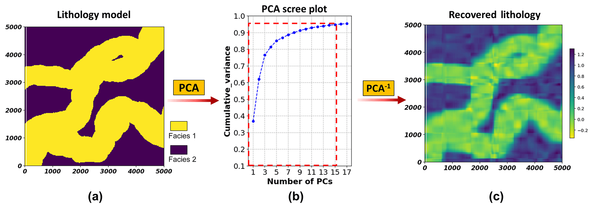
Figure 1 PCA on discrete lithology model: (a) the original lithology model; (b) scree plot of PCA on the lithology model. (c) The reconstructed model from inverse PCA using the preserved PCs (marked by the red dashed line on the scree plot).

2.3 Automation and code

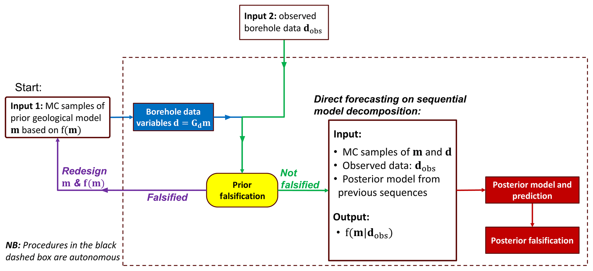
Our objective of automation is to allow for seamless uncertainty quantification once the prior uncertainty models have been established. Therefore, following the above-described geological UQ strategies, we design a workflow in Fig. 3 to automate the implementation. The workflow starts with the prior model Monte Carlo (MC) samples and borehole observations as input. All following steps including the extraction of borehole data variables, prior falsification, sequential direct forecasting, posterior prediction, and falsification (if required) are completely automated. With this workflow, we develop an open-source Python implementation to execute the automation (named “AutoBEL”). This open-source project can be accessed from Github (repository: https://github.com/sdyinzhen/AutoBEL-v1.0, last access: 13 January 2020, https://doi.org/10.5281/zenodo.3479997, Yin, 2019). Figure 4 briefly explains the structure of the Python implementation. Once a new borehole observation and prior model are provided from the “Input” directory, this automation implementation allows the uncertainty quantitation and updating to be performed automatically by running the Jupyter Notebook “Control panel”. The results from the automated uncertainty quantification are stored in the “Output”, classified as “Model”, “Data”, and “Prediction”.

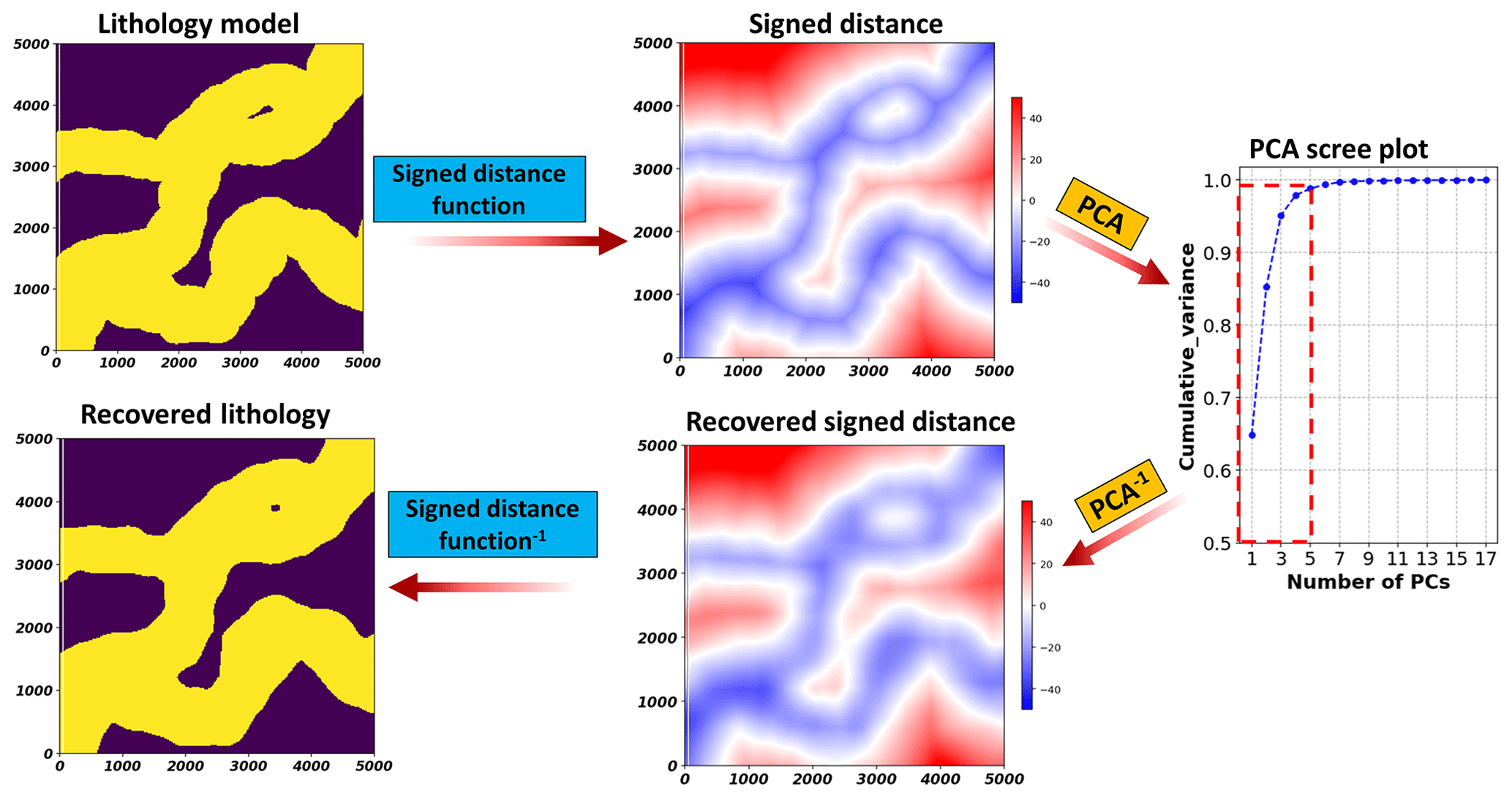
Figure 2 Example of transforming categorical lithology model to continuous signed distances for performing PCA.

Figure 3 Proposed workflow to automate the geological uncertainty quantification.

3 Application example

3.1 The field case

We demonstrate the application of the automated UQ framework using a synthetic dataset inspired by a gas reservoir located offshore of Australia. This case study is regarded as synthetic due to simplification for generic application and because of confidentiality issues. Its spatial size is around 50 km (E–W) ×25 km (N–S) with a thickness ranging from 75 to 5 m. The reservoir rocks are deposited in a shallow marine environment, with four lithological facies belts corresponding to four different types of porous rocks (Fig. 5a). The rock porous system contains natural gas and formation water. The major challenges lie in quantifying spatial geological uncertainty, appraising gas initially in place (GIIP), and then fast updating the uncertainty quantification when new boreholes are drilled. This will directly impact the economic decision making for reservoir development.

Figure 4 The structure of the AutoBEL python implementation project.

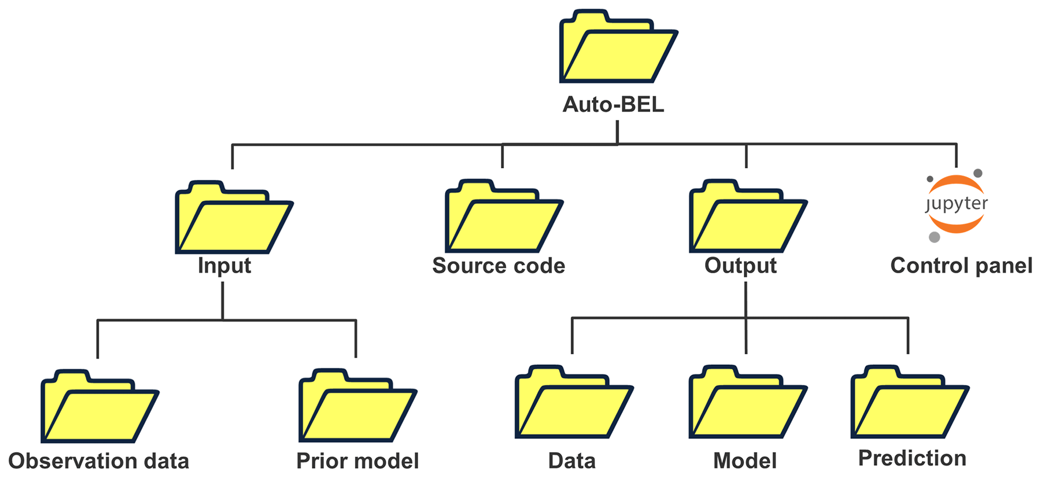
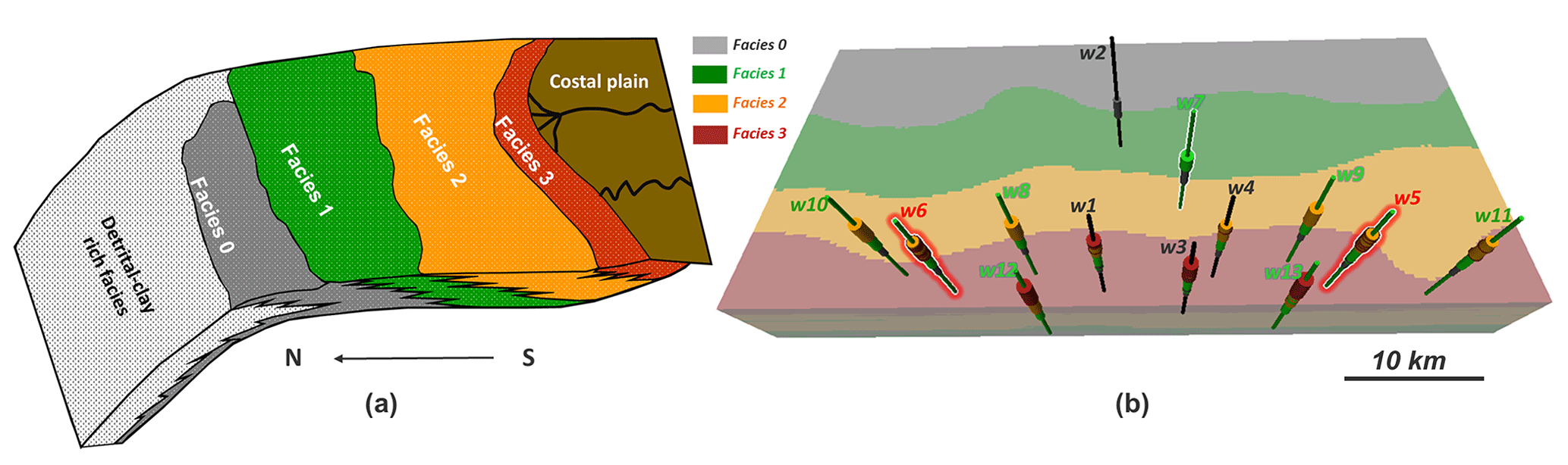
Figure 5 (a) The field geology conceptual model with the four facies belts. (b) The initial 3-D geological model of facies with locations of existing boreholes and newly drilled boreholes.

Initially, the reservoir geological variation is represented on a 3-D model (Fig. 5b) with a total of 1.5 million grid cells with dimension of $\mathrm{200}\times \mathrm{100}\times \mathrm{75}$ (layers). Companies often drill exploration and appraisal wells before going ahead with producing the reservoir. They would like to decrease uncertainty by such drilling to a point where the risk is considered tolerable to start actual production. To mimic such a setting, we consider that initially four well bores (w1, w2, w3, w4; marked in Fig. 5b) have been acquired and that models have been built using the data from these wells. Then nine new wells (w5 to w13 in Fig. 5b) are drilled, and uncertainty needs to be updated. The idea is to use the nine new wells to automatically update the reservoir uncertainty using the procedures developed above. In order to validate our results, we will use observations from w7 to w13 to reduce the uncertainty, whereas observations from w5 and w6 will be used to analyze the obtained uncertainty quantification.

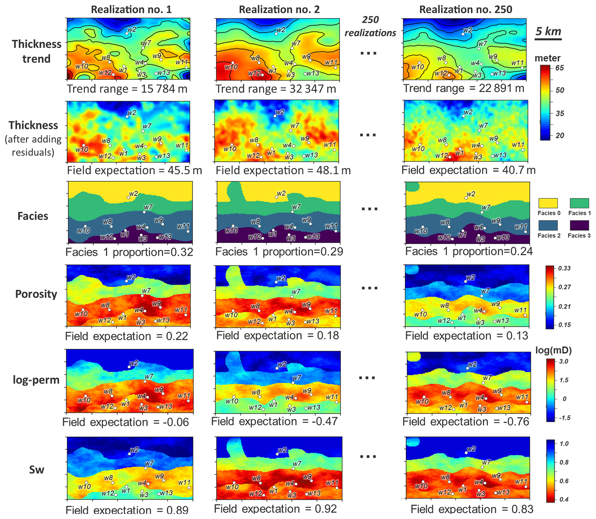
Figure 6 Layer view of prior Monte Carlo model samples of thickness trend and corresponding thickness, facies, porosity, permeability (logarithmic, termed log-perm), and Sw.

3.2 Prior model parameterization and uncertainty

3.2.1 Approaches

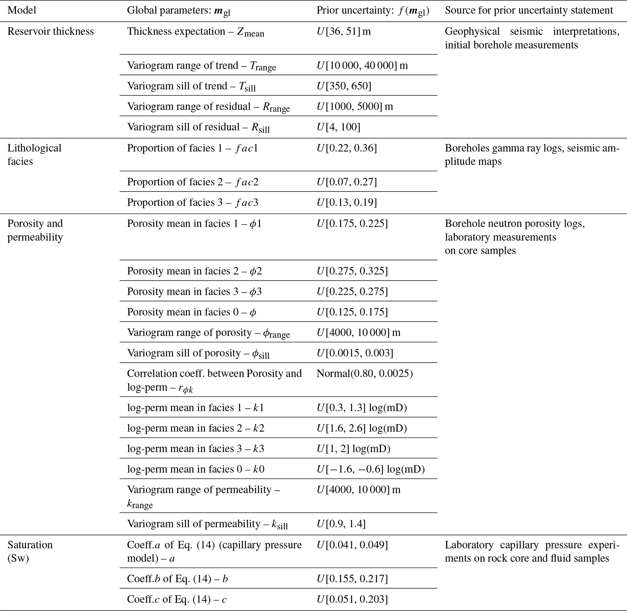
The reservoir geological properties responsible for reserve appraisals are spatial variations in (1) reservoir thickness, spatial distributions of (2) lithological facies belts, (3) 3-D porosity, and (4) 3-D formation water (saturation), while the spatial heterogeneity of (5) 3-D permeability is critical to the future production of gas but is not used in volume appraisal. Constructing a prior uncertainty model for these properties requires a balance between considering aspects of the data and overall interpretation based on such data. The strategy in the BEL framework is not to state too narrow an uncertainty initially but rather to explore a wide range of possibilities. Based on interpretation from data, Table 1 contains all uncertainties and their prior distribution was constructed. We will clarify how these uncertainties were obtained.

Table 1 The global model parameter m_gl and its prior uncertainty distribution f(m_gl). The initial prior distributions of the parameters are mostly assumed to be uniform (formulated as U[min, max]) due to limited available data.

Thickness

First, the thickness uncertainty is mainly due to a limited resolution of the geophysical seismic data and uncertainty in velocity modeling (not shown in this paper). Seismic interpretations show no faults in the geological system, but the thickness variations follow a structural trend. To model thickness uncertainty, we decompose thickness Z(x) into an uncertain trend T(x) and uncertain residual R(x):

$$\begin{array}{}\text{(13)}& Z\left(\mathit{x}\right)=T\left(\mathit{x}\right)+R\left(\mathit{x}\right).\end{array}$$

Note that most common geostatistical approaches do not consider uncertainty in trend. Uncertainty in T(x) can be estimated using geophysical data such as seismic, electrical resistivity tomography, or airborne electromagnetics. This case study uses seismic data. We describe uncertainty in the trend using a 2-D Gaussian process (Goovaerts, 1997) with uncertain expectation and spatial covariance. The expectation is interpreted from seismic data with a vertical resolution of 15 m, while the uncertain spatial covariance is modeled using a geostatistical variogram of seismic data with uncertain range (spatial correlation length) and sill (variance). The residual R(x) is modeled using a zero-mean 2-D Gaussian process with unknown spatial covariance. This term is highly uncertain, in particular the covariance, because the residual term is observed only at four initial borehole locations. However, the variogram range is assumed to be much smaller than the trend variogram, as residuals aim to represent more local features. Once the Gaussian process is defined, it can be constrained (conditioned) to the actual thickness observation at the vertical boreholes through the generation of conditional realizations. Note that these conditional realizations contain the uncertainties of trend and residual terms (Fig. 6).

Facies

The lithological facies are considered to have rather simple spatial variability and are described as “belts” (see Fig. 5a). These are common in the stratigraphic progression and typical of shallow marine environments. To describe such variation, we use a 3-D Gaussian process that is truncated (Beucher et al., 1993), thereby generating discrete variables. This truncated Gaussian process has a specific advantage in reproducing simple organizations of ordered lithologies, thus making a useful model in our case. Because four facies exist, three truncations need to be made on the single Gaussian field. The truncation bounds are determined based on facies proportions. The uncertain facies proportions are obtained from lithological interpretations on borehole gamma ray logs and geophysical seismic interpretation.

Porosity and permeability

For each facies belt, rock porosity and permeability (logarithmic scale, termed log-perm) are modeled, using two correlated 3-D Gaussian processes. The cross-covariances of these processes are determined via Markov models (Journel, 1999) that only require the specification of a correlation coefficient. Laboratory measurements on the borehole rock core samples show that permeability is linearly correlated to porosity with a coefficient of 0.80 and a small experimental error (around 6 % random error according to the lab scientists by repeating the experiments). The marginal distributions of porosity and log-perm are assumed to be normal but with uncertain mean and variances. The mean of porosity and log-perm is based on borehole neutron porosity logs and core sample measurements. Similar to the thickness residual modeling, the spatial covariances are modeled via a variogram, respectively, for porosity and permeability, with uncertain range and sill. Limited wellbore observations make variogram range and sill highly uncertain, and therefore large uncertainty bounds are assigned.

Saturation

Rocks contain gas and water; hence the uncertain saturation of water (Sw) will affect the uncertain gas volume calculations. The modeling of Sw is based on a classical empirical capillary pressure model from a Leverett J-function (Leverett et al., 1942), formulated as

$$\begin{array}{}\text{(14)}& \mathrm{Sw}={\mathrm{10}}^{-a\cdot {\left[\log \left(j\right)\right]}^{\mathrm{2}}-b\cdot \log \left(j\right)-c},\end{array}$$

where $j=\mathrm{0.0055}\cdot h\sqrt{\mathrm{\varnothing }/k}$ and h is height above the reservoir free water level. The uncertainty parameters in this fluid modeling are the coefficients a, b, and c. Their prior distributions are provided by capillary pressure experiments using rock core plugs and reservoir fluids as shown in Table 1.

3.2.2 Monte Carlo

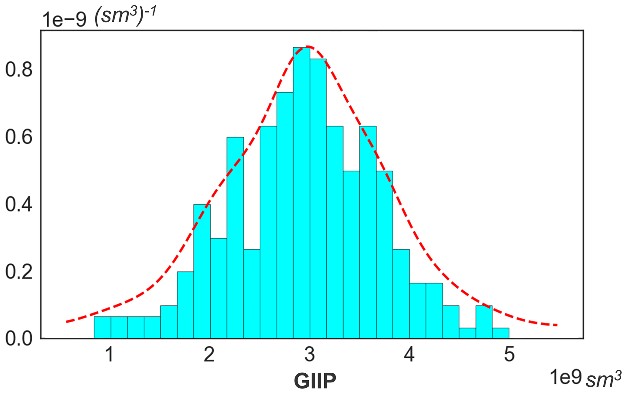
By running Monte Carlo from the given prior distribution in Table 1, a set of 250 geological model realizations are generated. Figure 6 displays Monte Carlo realizations of the geological model: thickness trend and corresponding thickness model, facies, porosity, permeability (log-perm), and Sw. With prior samples of the geological model, prior prediction of GIIP is calculated, using the following linear equation:

$$\begin{array}{}\text{(15)}& \mathrm{GIIP}=\text{study area}\cdot \text{thickness}\cdot \text{porosity}\cdot (\mathrm{1}-\mathrm{Sw})/\mathrm{Bg},\end{array}$$

where the Bg is the gas formation volume factor provided from laboratory measurements. The calculated GIIP prediction is plotted in Fig. 7. The plot shows that the initial prediction of reservoir gas storage volume has a wide range, which means a significant risk can exist during decision making for field development.

Figure 7 Uncertainty quantification of GIIP based on prior uncertainty and four boreholes.

3.3 Prior falsification with newly acquired borehole data

Table 1 is a subjective statement of prior uncertainty. When new data are acquired, this statement can be tested, using a statistical test (Sect. 2.1.3) that may lead to a falsified prior. To perform falsification, borehole data variables at the seven new well locations (from w7 to w13) are extracted by applying the data forward operator G_d to the 250 prior model realizations. It simply means extracting all thickness, facies, petrophysics, and saturation at the borehole locations in the prior model. For the 2-D thickness model, the new boreholes provide seven data extraction locations. For the 3-D model of facies, porosity, permeability, and Sw, each vertical borehole drills through 75 grid layers; thus the seven boreholes provide 2100 extracted data measurements (75 data measurements/well ×7 wells ×4 model components =2100 data measurements). The dimensionality of data variable d in this case therefore equals 2107. The actual observations of these data (d_obs) are measured from the borehole wireline logs and upscaled to the model resolution vertically. As described in Sect. 2.1.3, prior falsification is then conducted by applying the robust Mahalanobis distance outlier detection to d and d_obs. Figure 8 shows the calculated RMD for d_obs and the 250 samples of d, where the distribution of the calculated RMD(d) falls to a chi-squared distribution, with the RMD(d_obs) falling below the 97.5 percentile threshold. This shows with (97.5) confidence that the prior model is not wrong.

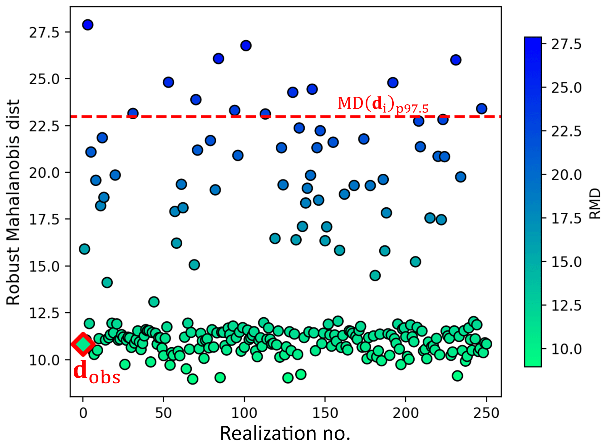
Figure 8 Prior falsification using robust Mahalanobis distance (RMD). Circle dots represent the calculated RMD for data variable samples. The red square is the RMD for borehole observations. The red dashed line is the 97.5 percentile of the chi-squared distributed RMD.

3.4 Automatic updating of uncertainty with new boreholes

After attempting to falsify the prior uncertainty model, we use the automated framework to jointly update model uncertainty with the new boreholes. The joint model uncertainty reduction is performed sequentially as explained in Sect. 2.2.2. Under the AutoBEL GitHub repository instruction (https://github.com/sdyinzhen/AutoBEL-v1.0/blob/master/README.md, last access: 13 January 2020), we also provide a supplement YouTube video to demonstrate how this automated update is performed.

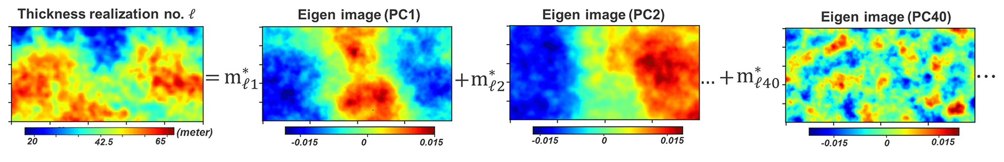
Figure 9 Example of applying PCA to thickness model. One model realization l ($l=\mathrm{12},\mathrm{\dots }L$) can be represented by the linear combination of eigen images scaled by the PC scores ${\mathit{m}}_l^{\ast }$.

3.4.1 Thickness and facies

Uncertainty in facies and thickness models can be updated jointly, as they are two independent components for this case. AutoBEL first transforms the categorical facies to a continuous model using signed distance function. The transformed signed distances are then combined with the thickness model to perform orthogonalization using mixed PCA (Abdi et al., 2013). As shown in Fig. 9, the first eigen image (first principal components, PC1) of thickness reflects the global variations in reservoir thickness, while higher-order eigen images (e.g., eigen image of PC40) represent more local variation features. To evaluate what model variables impact thickness variation at the boreholes, DGSA (Fenwick et al., 2014) is then performed to analyze the sensitivity of model variables to data. Figure 10a plots the main effects in a Pareto plot. As shown in the plot, DGSA identifies sensitive (measure of sensitivity >1) and non-sensitive (measure of sensitivity <1) model variables. Thickness global parameters of both trend (Z_mean, T_range, T_sill) and residuals (R_range) show sensitivity to the borehole data. In terms of facies, proportions of the facies 1 (fac1) and 2 (fac2) are sensitive. There are, in total, 26 sensitive principal components from the spatial model. These sensitive global variables and principal component scores are now selected for uncertainty quantification.

Following the steps of direct forecasting (see Sect. 2.2.1), uncertainty reduction proceeds by mapping all sensitive model variables into a lower-dimensional space such that the Bayes–linear-Gauss model can be applied. This requires the application of CCA to the selected model variables and data variables and then normal score transformation. Figure 10b shows two examples of a cross plot between model and data variables of the first and tenth canonical components, where we observe a linear correlation coefficient of 0.84 even for the tenth canonical components. Once the Bayesian model is specified, one can sample from the posterior distribution and back-transform from lower-dimensional scores into actual facies and thickness models. Figure 10c shows the distribution of the posterior model realizations in comparison to the corresponding prior, showing the reduction in the model uncertainty. Figure 10d shows the comparison between the prior and posterior distributions of the scores for the first four sensitive PCs, where the reduction in uncertainty is observed (while noting that uncertainty quantification involves all the sensitive PC score variables).

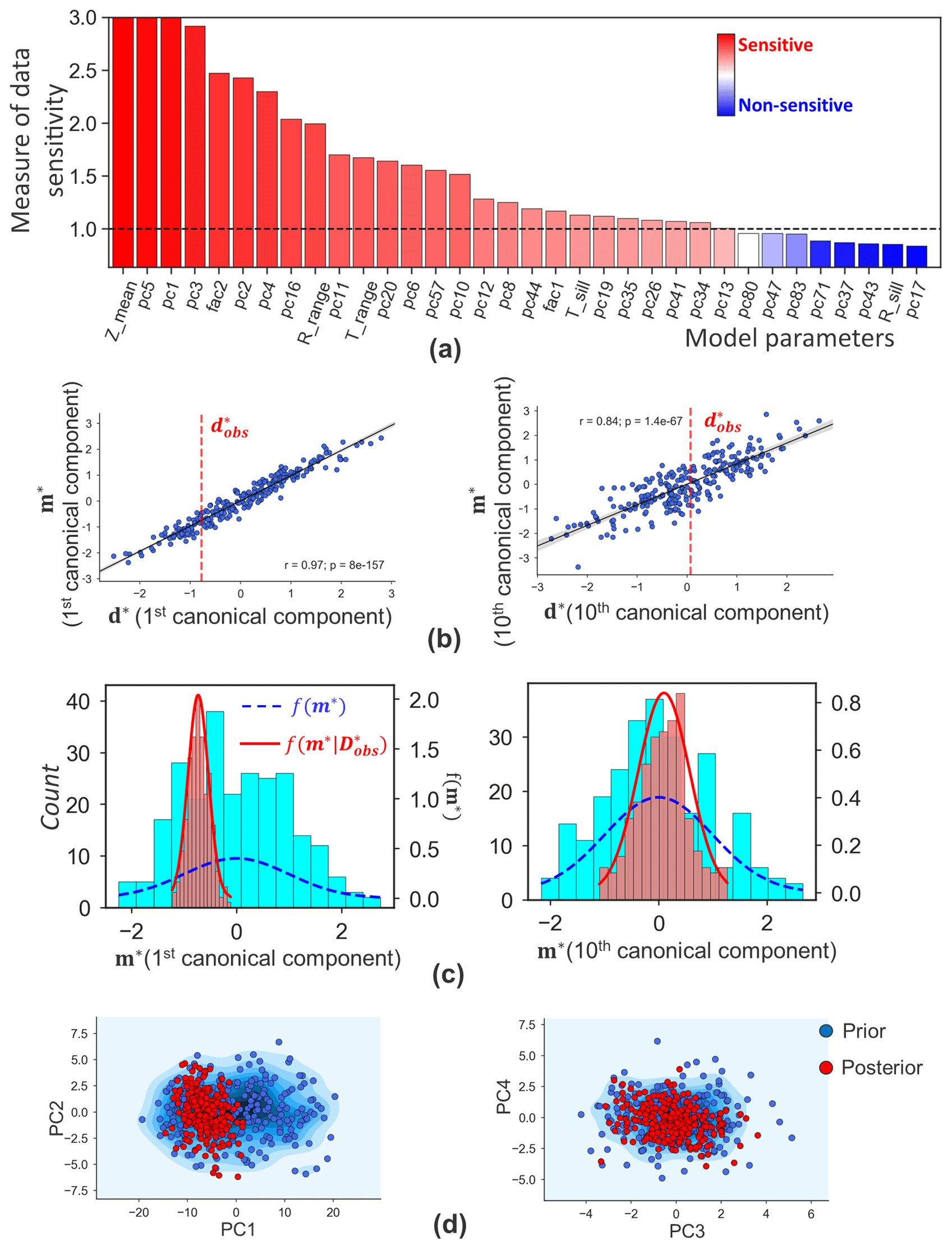
Figure 10 Uncertainty reduction in thickness and facies: (a) global sensitivity of model parameters to borehole data. (b) First and tenth canonical covariates of data and model variables. The dashed red line is the observation data. (c) Posterior and prior distributions of model variables (first and tenth canonical components, corresponding to b). (d) Prior and posterior PC score distributions of first four sensitive PCs.

Figure 11 plots the reconstructed posterior global parameters in comparison to the prior. Uncertainty reduction in sensitive global parameters is observed, while the distribution of non-sensitive global parameters (R_sill and fac3) is unchanged. To assess the reconstructed posterior spatial model realizations, we calculate the mean for thickness (namely “ensemble mean”) and the median realization of facies. Variance is also calculated for thickness and facies, respectively (“ensemble variance”). Figure 12 shows show the ensemble mean and median of the thickness and facies realizations, while the ensemble variances is shown in Fig. 13. The results in Fig. 12 imply that the posterior model thickness is thicker on average than the prior. This change mainly occurs in areas where the new boreholes are drilled. Referring to the actual borehole observations plotted in Fig. 12, we also find that the posterior thickness adjusts to the borehole observations at both training (w7–w13) and validating (w5, w6) locations. This improvement is significant compared to the prior model. Furthermore, the ensemble variances (Fig. 13) are reduced in the posterior model, mostly in the vicinity of the new boreholes. This implies a reduction in the spatial uncertainty. One should note that our method does not (yet) result in an exact match of the thickness with borehole data. This is an issue we will comment on in the Discussion section and the Conclusion. For the facies model, the magnitudes of the uncertainty reduction are not as remarkable because prior uncertainty at borehole locations was small to start with.

Figure 11 Uncertainty updating of (a) sensitive and (b) non-sensitive global model parameters at the first sequence. The dashed lines are estimated kernel density with Gaussian kernels.

3.4.2 Porosity, permeability, and saturation

AutoBEL is now applied to update the uncertainty in porosity, permeability, and saturation under the sequentially decomposition.

The prior Monte Carlo samples have provided a full distribution of porosity for each facies. This allows the calculation of posterior porosity to fit the obtained posterior facies models. Therefore, we condition to posterior facies model and borehole porosity observations in AutoBEL to calculate the posterior porosity. Similarly, for permeability and saturation model, AutoBEL is applied by additionally conditioning to posterior models from previous model components.

Figures 14, 15, and 16 show the results. In Fig. 14, we see sensitive global and spatial model variables that are selected for uncertainty reduction. Figure 15 shows the constructed the linear correlation between data and sensitive model variables by means of CCA. Figure 16 plots the posterior model realizations (250 realizations) computed from the Bayes–linear-Gauss model, where reduced uncertainty is observed when comparing to the prior. The posterior spatial model PC scores are also plotted in Fig. 17.

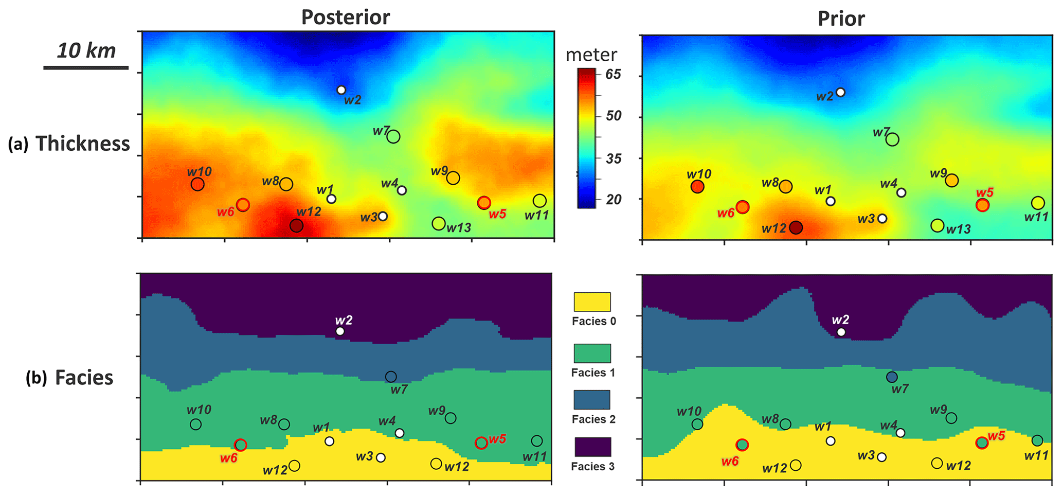
Figure 12 (a) Ensemble mean of posterior and prior thickness. (b) The median realization of posterior and prior facies. The dots are borehole locations and their color represents the actual borehole observation values. The boreholes and models share the same color legend.

Figure 13 Ensemble variance of the posterior and prior thickness and facies models from the first sequence.

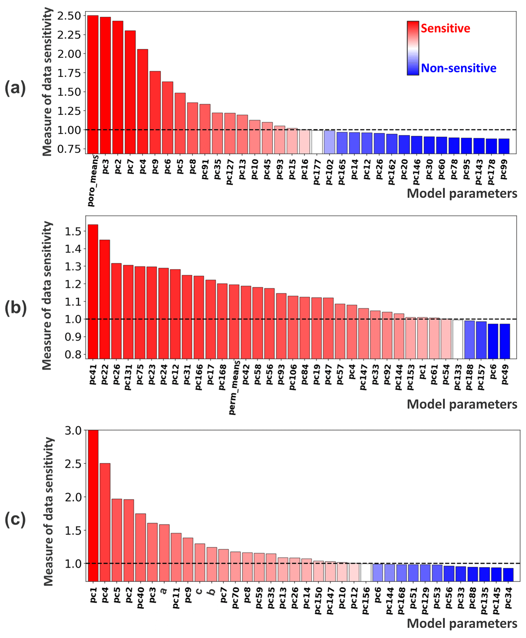
Figure 14 Results from global sensitivity analysis using DGSA at (a) porosity,, (b) log-perm and (c) Sw.

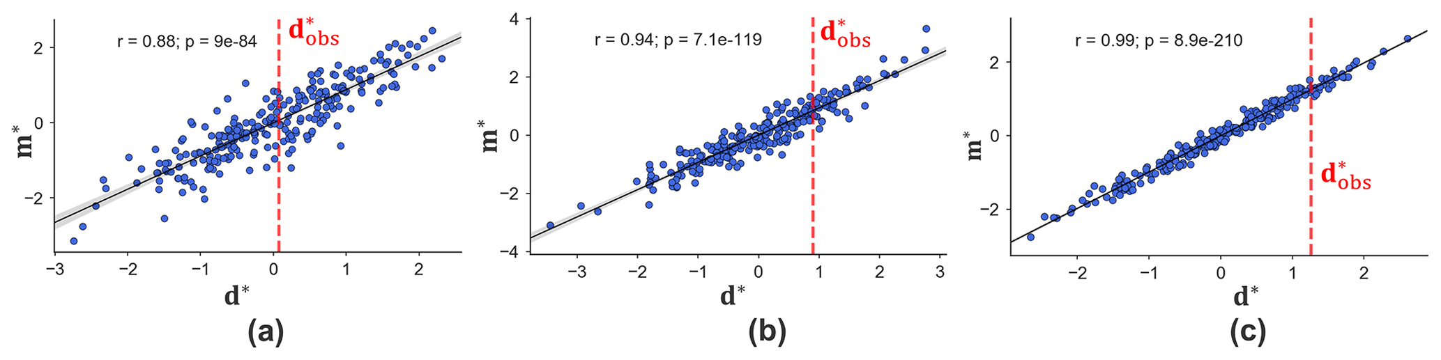
Figure 15 First canonical covariates of data and model variables from (a) porosity, (b) log-perm, and (c) Sw.

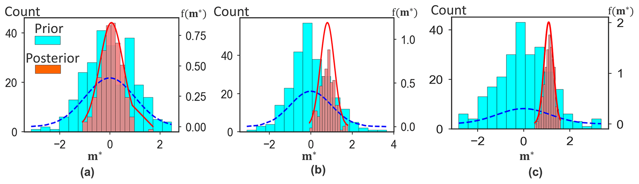
Figure 16 Reduction in uncertainty of the first model canonical component: (a) porosity, (b) log-perm, and (c) Sw.

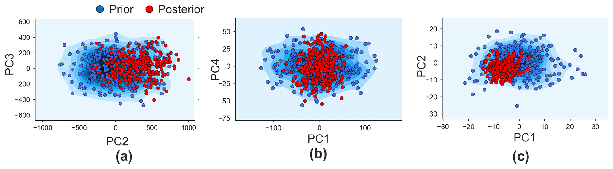
Figure 17 Prior and posterior distribution of the scores of the two sensitive PCs with highest variances: (a) porosity, (b) log-perm, and (c) Sw.

Finally, by back-transformation, we can reconstruct all original model variables. Figure 18 compares ensemble means and variances of the reconstructed posterior porosity, log-perm, and Sw to their corresponding prior models, with actual borehole observations plotted on top. Taking w7 for example, the actual borehole observations show low values of porosity, permeability, and Sw, while the prior model initially expects those values to be large at this location. This is adjusted in the posterior. From the ensemble variance maps, we notice that spatial uncertainty is significantly reduced from prior to posterior in areas near w7. The updates of model expectations and reduction in spatial uncertainty are also observed from the other wells. It implies that the posterior models have been constrained by the borehole observations.

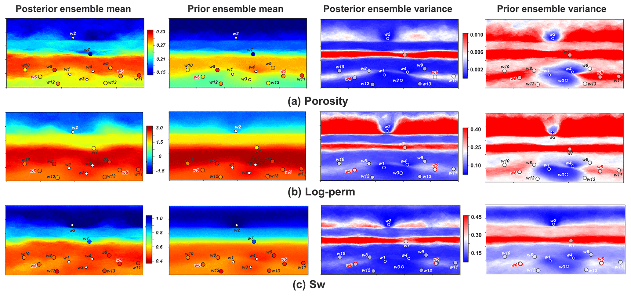
Figure 18 Ensemble mean and variance of posterior and prior geological models: (a) porosity; (b) log-perm; (c) water saturation. The dots represent locations of the boreholes, where the color of the dots represents observation values.

Figure 19 shows one example realization of the spatial models. It shows that, as with the hierarchical order in the prior (Fig. 19a), the spatial distributions of posterior porosity and log-perm follow the spatial patterns of their corresponding facies belts (Fig. 19b). However, if the joint model uncertainty reduction is performed without the sequential decomposition (not conditioning to the posterior models from previous sequences), the model hierarchy from facies to porosity and permeability is lost (marked by the purple boxes in Fig. 19c). This is because they are treated as independent model variables, which violates the imposed geological order of variables. The linear correlation between porosity and log-perm is also preserved due to the sequential decomposition. We observe similar correlation coefficients from prior (Fig. 20a) to posterior (Fig. 20b). But without sequential decomposition, this important feature cannot be maintained as the results shown from Fig. 20c: (1) the four-cloud pattern (representing the four facies) of the covariate distribution between porosity and log-perm is lost; (2) the correlation coefficient has changed significantly for facies 0, 2, and 3.

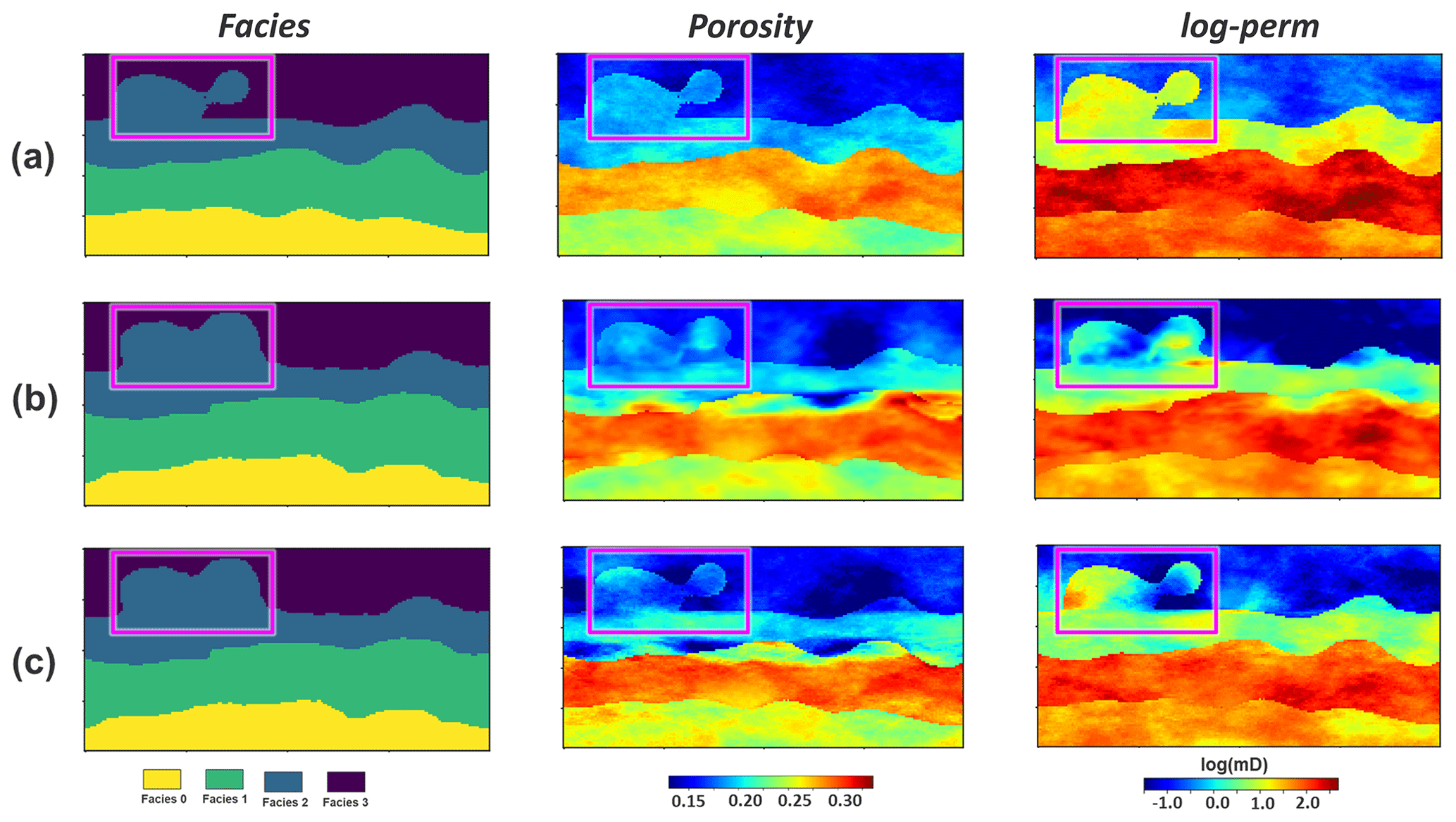
Figure 19 Prior and posterior facies, porosity and log-perm of realization no. 1 (a) prior model; (b) posterior model from the sequential decomposition; (c) posterior from joint uncertainty reduction without sequential decomposition.

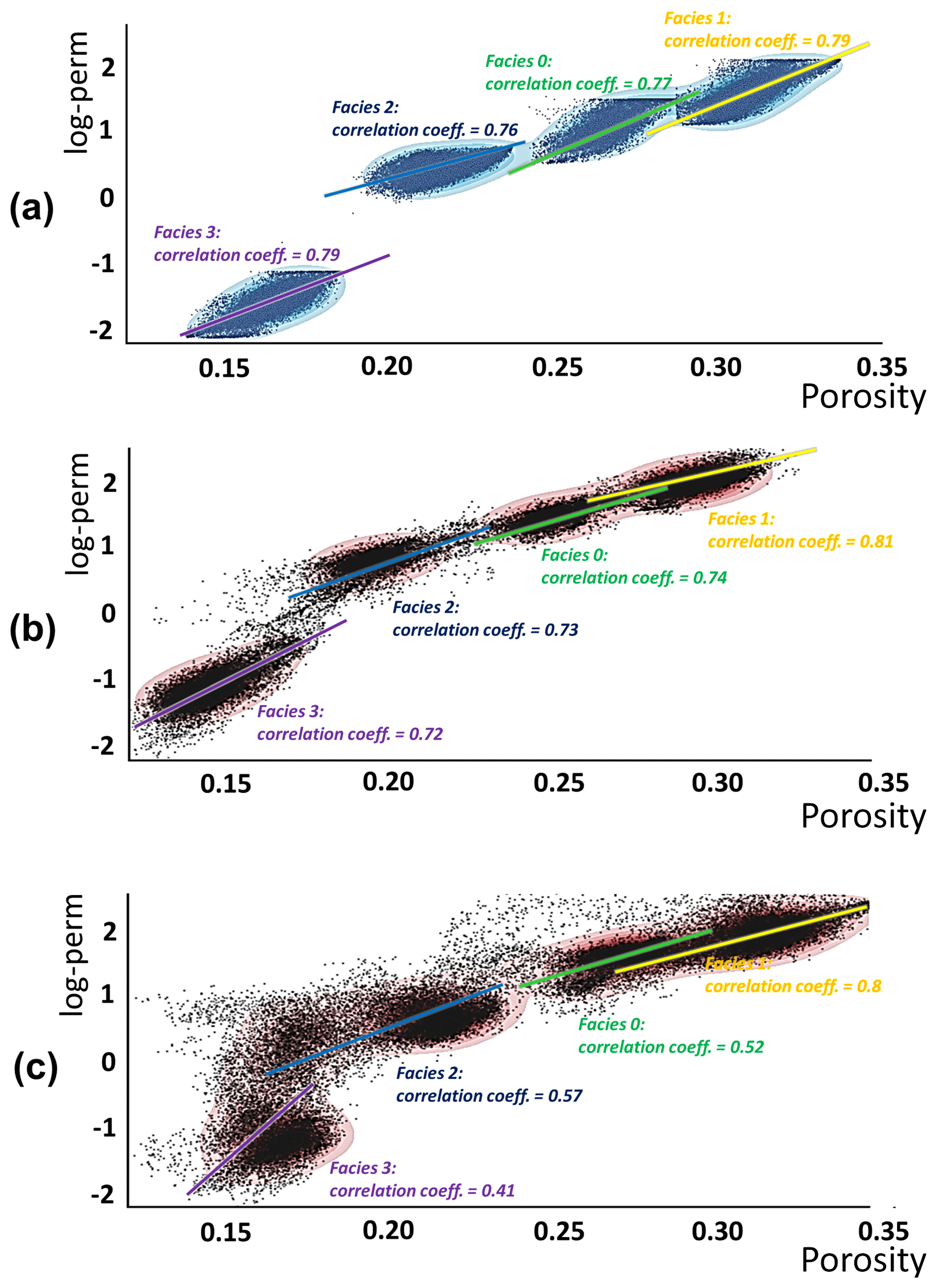
Figure 20 Bivariate distribution between porosity and log-perm model of realization no. 1 (a) prior, (b) posterior from the sequential decomposition, (c) posterior without performing sequential decomposition. The correlation coefficient is examined for each facies.

3.4.3 Posterior prediction and falsification

Gas storage volume is calculated using the posterior geological models and plotted in Fig. 21. The result highlights a steep uncertainty reduction in comparison to the initial prior prediction. The posterior predicted GIIP leads to a major shift in the expected gas volumes to a more positive direction (higher than initially expected). More importantly, the forecast range is significantly narrowed. This provides critical guidance to the financial decisions on the field development. It also in return confirms the value of the information of the newly drilled wells. In total, the whole application of AutoBEL to this test case took about 45 min (not including the time on prior modeling) when run on a laptop with an Intel Core i7-7820HQ processor and 64 GB of Ram.

To test the posterior, we perform posterior falsification using data from validating boreholes (w5 and w6). Figure 22 plots the result from applying robust Mahalanobis distance outlier detection to the posterior data of the two wells. The statistical test shows that the test borehole observation falls within the main population of data variables, below the 97.5 threshold percentile. We also want to further examine if the posterior models can predict the validating boreholes (regarded as future drilling wells) with reduced uncertainty. To do so, we compare the prior and posterior predicted thickness at the two borehole locations, together with their actual measurements (Fig. 23). For 3-D models of facies, porosity, log-perm, and Sw, this comparison is performed on vertical average values across the 75 layers. We notice that these future borehole observations are predicted by posterior models with significantly reduced uncertainty.

4 Discussion

One main purpose of this paper is to introduce automation to geological uncertainty quantification when new borehole data are acquired. We tackle this challenge by following the protocol of Bayesian evidential learning to build an automated UQ framework. BEL formulates a protocol involving falsification, global sensitivity analysis, and statistical learning uncertainty reduction. When establishing such a framework for geological UQ, three important questions have to be addressed. The first is on how to preserve the hierarchical relationships and correlations that commonly exist in geological models. We propose a sequential decomposition by following the chain rule under Bayes' theorem. This allows us to assess the joint distribution of multiple model components while honoring the geological rules. The second one is on how to falsify the geological model hypotheses, especially when data become highly dimensional. We employ multivariate outlier detection methods. They provide quantitative and robust statistical calculations when attempting to falsify the model using high-dimensional data. The last but most practical one, is to deploy data-science-driven uncertainty reduction. Uncertainty reduction in geological models is usually time-consuming because conventional inverse methods require iterative model rebuilding. When it comes to real cases, the daunting time consumption and computational efforts of conventional methods can hamper practical implementations of automation. Direct forecasting helps to avoid this, as it mitigates the uncertainty reduction to a linear problem in a much lower dimension. There are many dimension reduction methods for complex models, such as deep neural network (Laloy et al., 2017, 2018), but here we use PCA because it is simple and bijective, and the structure models are not complex (e.g., channels). However, direct forecasting of geological model is faced with two new challenges. One is to accommodate a direct forecasting algorithm to the sequential model decomposition. This is achieved by additionally conditioning to the posterior from previous sequences. The other challenge is that DF cannot be directly applied to categorical models such as lithological facies. We therefore introduce a signed distance function to convert categorical models to continuous properties before performing the DF. Field application has shown the benefits of using the proposed framework. Since the posterior in the case study cannot be falsified, its uncertainty can be further reduced by repeating the automated procedures with validating borehole observations. This suggests that the proposed framework has potentials for life-of-field uncertainty quantification for applications where new boreholes are regularly drilled.

The main challenge addressed in this paper is to apply such an uncertainty quantification within a Bayesian framework. Most methods applied in this context simply rebuild the models by repeating the same geostatistical methods that were used to construct the prior model. In such an approach, all global variables and their uncertainty need to be reassessed. The problem with such an approach is twofold. First, it does not address the issue of falsification: the original models may not be able to predict the data. Hence, using the same approach to update models with a prior that may have been falsified may lead again to falsification, thereby leading to invalid and ineffective uncertainty quantification. As a result, the uncertainty quantification of some desirable property, such as volume, exhibits a yo-yo effect (low variance in each UQ but shifting mean). Second, there is no consistent updating of global model variables. Often such uncertainties are assessed independently of previous uncertainties. The challenge addressed in this paper is to jointly update global and spatial variables and do this jointly for all properties.

The proposed method offers a Bayesian consistency to uncertainty quantification in the geological modeling setting. However, unlike geostatistical methods, the posterior models do not fully match local borehole observations. The current method is only designed to globally adjust the model, not locally at the borehole observation. This can be an important issue if using the model for subsurface flow simulations. To tackle this problem, one possible path we would like to explore in the future is to combine geostatistical conditional simulation as posterior step to the current methodology. A second limitation is that the method does not (yet) treat discrete global variables, such as a geological interpretation. In the case study, only one interpretation of the lithology was used. The way such variables would be treated is by assigning prior probabilities to each interpretation (e.g., of a depositional system) and then updating them into posterior probabilities. This has been done by treating the interpretation independent of other model variables in some studies (e.g., Aydin and Caers, 2017; Grose et al., 2018; Wellmann et al., 2010). For example, one could first update the probabilities of geological scenarios, then update the other variables (Lopez-Alvis et al., 2019). Regarding the automation of BEL, its intermediate steps can also be adjusted depending on users' specific applications. Taking the direct forecasting step for example, here we adapt it for uncertainty quantification using borehole data, which is a linear problem. But for more complex nonlinear inverse problems, it may be difficult to use CCA to derive a Bayes–linear-Gauss relationship in DF. Statistical estimation approaches such as kernel density estimation (Lopez-Alvis et al., 2019) can be used for such cases, and there are also extensions of CCA to tackle nonlinear problems (e.g., Lai and Fyfe, 1999). AutoBEL can also be adapted if other types of parameters (other than spatial model parameters) are used for uncertainty quantification. This can be done by simply adding the additional parameters to the model variable m. A final, and perhaps more fundamental, concern not limited to our approach is what should be done when the prior model is falsified with new data. According to the Bayesian philosophy this would mean that any of the following could have happened: uncertainty ranges are too small, the model is too simple, or some combination of both. The main problem is that it is difficult to assess what the problem is exactly. Our future work will focus on this issue.

Figure 21 The prior and posterior prediction of GIIP.

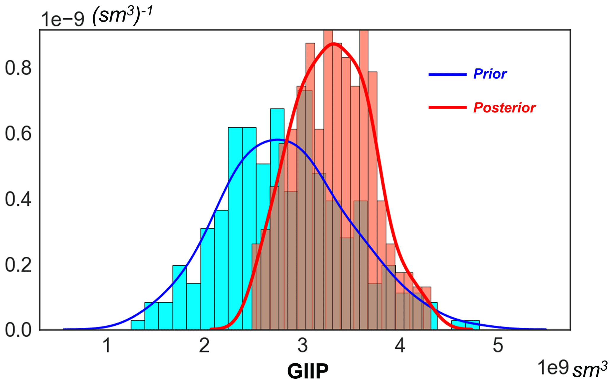
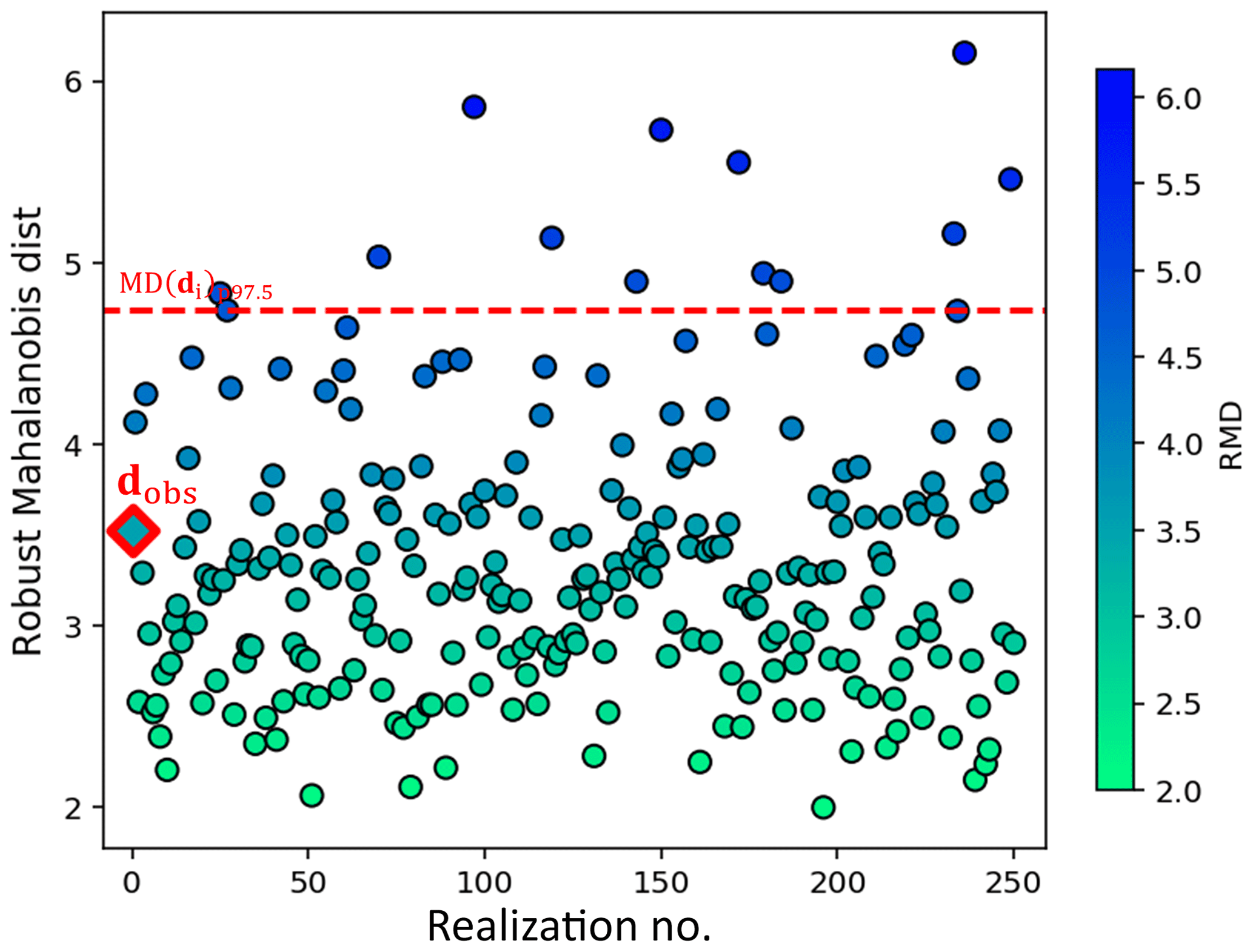
Figure 22 Posterior falsification using robust Mahalanobis distance outlier detection method using the data from w5 and w6.

Figure 23 Prior and posterior predicted thickness, facies, porosity, log-perm, and Sw at validating boreholes. The blue and brown colored dots, respectively, represent the prior and posterior prediction, while the red squares are the actual observations.

5 Conclusions

In conclusion, we generalized a Monte Carlo-based framework for geological uncertainty quantification and updating. This framework, based on Bayesian evidential learning, was demonstrated in the context of geological model updating using borehole data. Within the framework, a sequential model decomposition was proposed, to address the geological rules when assessing the joint uncertainty distribution of multiple model components. For each component, we divided model parameters into global and spatial ones, thus facilitating the uncertainty quantification of complex spatial heterogeneity. When new borehole observations are measured, instead of directly reducing model uncertainty, we first strengthen the model hypothesis by attempting to falsify it via statistical tests. Our second contribution was to show how direct forecasting can jointly reduce model uncertainty under the sequential decomposition. This requires a posterior model from previous sequences as additional inputs to constrain the current prior. Such sequential direct forecasting was shown to maintain important geological model features of hierarchy and correlation, whilst avoiding the time-consuming conventional model rebuilding. In terms of discrete models, such as lithology, a signed distance function was employed, before applying direct forecasting to reduce uncertainty. The third contribution, but maybe a more important one, is that the proposed framework allows the automation of geological UQ. We developed an open-source Python project for this implementation. Its application to a large reservoir model showed that the automated framework ensures that the model is objectively informed by data at each step of uncertainty quantitation. It jointly quantified and updated uncertainty of all model components, including structural thickness, facies, porosity, permeability, and water saturation. The posterior model was shown to be constrained by new borehole observations globally and locally, with dependencies and correlations between the model components preserved from the prior. It predicted validating observations (future drilling boreholes) with reduced uncertainty. Since the posterior cannot be falsified, the uncertainty-reduced GIIP prediction can be used for decision makings. The whole process takes less than 1 h on a laptop workstation for this large field case, thus demonstrating the efficiency of the automation