the Creative Commons Attribution 4.0 License.
the Creative Commons Attribution 4.0 License.
 | 11 Dec 2020
Description of the uEMEP_v5 downscaling approach for the EMEP MSC-W chemistry transport model
Michael Gauss
Peter Wind
Eivind Grøtting Wærsted
Hilde Fagerli
Alvaro Valdebenito
Heiko Klein
A description of the new air quality downscaling model – the urban EMEP (uEMEP) and its combination with the EMEP MSC-W model (European Monitoring and Evaluation Programme Meteorological Synthesising Centre West) – is presented. uEMEP is based on well-known Gaussian modelling principles. The uniqueness of the system is in its combination with the EMEP MSC-W model and the “local fraction” calculation contained within it. This allows the uEMEP model to be imbedded in the EMEP MSC-W model and downscaling can be carried out anywhere within the EMEP model domain, without any double counting of emissions, if appropriate proxy data are available that describe the spatial distribution of the emissions. This makes the model suitable for high-resolution calculations, down to 50 m, over entire countries. An example application, the Norwegian air quality forecasting and assessment system, is described where the entire country is modelled at a resolution of between 250 and 50 m. The model is validated against all available monitoring data, including traffic sites, in Norway. The results of the validation show good results for NO2, which has the best known emissions, and moderately good for PM10 and PM2.5. In Norway, the largest contributor to PM, even in cities, is long-range transport followed by road dust and domestic heating emissions. These contributors to PM are more difficult to quantify than NOx exhaust emission from traffic, which is the major contributor to NO2 concentrations. In addition to the validation results, a number of verification and sensitivity results are summarised. One verification showed that single annual mean calculations with a rotationally symmetric dispersion kernel give very similar results to the average of an entire year of hourly calculations, reducing the runtime for annual means by 4 orders of magnitude. The uEMEP model, in combination with EMEP MSC-W model, provides a new tool for assessing local-scale concentrations and exposure over large regions in a consistent and homogenous way and is suitable for large-scale policy applications.
- Article
(2362 KB) - Full-text XML
-
Supplement
(1734 KB) - BibTeX
- EndNote


The EMEP MSC-W model is a chemistry transport model which has been developed by the Meteorological Synthesizing Centre – West (MSC-W) of EMEP, the European Monitoring and Evaluation Programme, under the UN Convention on Long-range Transboundary Air pollution (LRTAP). It is documented in Simpson et al. (2012) and has been used for many years mainly for regional but also for global applications. The aim of uEMEP (urban EMEP) is to further extend the application of the EMEP MSC-W chemical transport model down to near-street-level modelling. The downscaling methodology builds on classical Gaussian plume modelling and is integrated with the EMEP MSC-W model physical parameterisations and emission data in such a way as to provide a consistent model description from regional to local scales. Unlike other urban-scale models, uEMEP is intended not just to achieve local-scale modelling for an individual city or area but to provide local-scale modelling over entire countries or continents, providing high-resolution modelling over large areas and allowing air quality assessment and exposure calculations at high resolution everywhere. Air quality modelling is often separated into global, regional, urban and local scales. In this context, “local” refers to the ability of the model not just to represent urban background concentrations but also to represent street-level concentrations. There are a number of models that span the global or regional scale where grid resolutions down to 4–10 km have been achieved, e.g. EMEP MSC-W (Simpson et al., 2012; Werner et al., 2018), CHIMERE (Menut et al., 2013), SILAM (Sofiev et al., 2015), LOTOS-EUROS (Kranenburg et al., 2013), MATCH (Andersson et al., 2007) and CMAQ (Appel et al., 2017). There are a number of Gaussian modelling systems that cover the urban and local scales over limited areas, usually individual cities, e.g. ADMS (Stocker et al., 2012) and AERMOD (Cimorelli et al., 2004). In addition, there are some limited area models that combine Eulerian and Gaussian plume type models in a single system, e.g. Karamchandani et al. (2009), Kim et al. (2018) and Karl et al. (2019). If the full model cascade is to be achieved, such as the THOR forecast system in Denmark (Brandt et al., 2001), then this requires linking different model systems together to achieve high-resolution calculations in a limited area. An alternative approach to achieving high-resolution concentration fields over large regions without the use of chemistry transport models (CTMs) (Chemical transport models) are land use regression methods (e.g. Vizcaino and Lavalle, 2018); however, their lack of underlying physics does not make them useful for planning or policy applications.
Earlier work on the downscaling of CTMs over large regions include the population covariance correction factor from Denby et al. (2011) and the dispersion kernel methods from Theobald et al. (2016) and Maiheu et al. (2017). There are similarities between uEMEP and these last two studies as both use Gaussian models for the downscaling. The major difference between uEMEP and these two Gaussian kernel methods is that uEMEP can be applied on hourly data, as well as annual data, and that uEMEP is integrated with the “local fraction” scheme in EMEP MSC-W (Wind et al., 2020) that avoids double counting of emissions in a consistent manner.
In this paper, we provide an overall description of the uEMEP methodology and how it is combined with the “local fraction” scheme in EMEP MSC-W (Sect. 2). The uEMEP model physical parameterisations are then given in Sect. 3. In Sect. 4, an application example of the methodology, the Norwegian air quality forecasting service, is described. Validation of the modelling system against all Norwegian monitoring data is presented in Sect. 5 together with a summary of verification and sensitivity studies. Various aspects of the modelling are discussed in Sect. 6 and conclusions made in Sect. 7. More detailed information on the parameterisations, validation and verification is also provided in the Supplement.
In this section, we describe the concepts and methodologies for the application of the coupled modelling system uEMEP and EMEP MSC-W.
2.1 Overall concept and methodology
uEMEP provides a consistent methodology for redistributing/downscaling gridded CTM emissions and concentrations, in this case from the EMEP MSC-W model, to higher-resolution subgrids within the CTM grids. Proxy data, that represent the spatial distribution of the emissions, are used to redistribute emissions to subgrids. Concentrations are then recalculated at the subgrid level, using a Gaussian model, whilst removing the local contribution of the CTM at these subgrids but keeping the non-local contributions. This procedure consistently avoids double counting of emissions.
Throughout this paper, we refer to the downscaling grids in uEMEP as “subgrids”. These may be any size but current applications use a range of between 25 and 250 m. When referring to the EMEP MSC-W model, we use the term “grid”. This may also vary dependent on the application but is usually in the range of 2 to 15 km. The term “local” is also used. Local, in regard to EMEP, means the local EMEP grids, so terms such as “local fraction” refer to a particular grid and the other EMEP grids in the “local region”, for example, within a range of 5×5 EMEP grids. When referring to “local” in uEMEP, we also refer to subgrid contributions from within this local EMEP region. This is visualised in Fig. 1. “Non-local”, in regard to uEMEP, refers to any contribution that is not downscaled or calculated with uEMEP, usually contributions from outside the local EMEP region but these can also be other source sectors not accounted for by uEMEP. We will refer to concentrations provided by the EMEP MSC-W model simply as EMEP concentrations.
uEMEP can be run using two downscaling methods, both of which make use of Gaussian dispersion modelling to describe the redistribution of concentrations at high resolution. Both methods make use of the recently developed “local fraction” functionality in the EMEP model (Sect. 2.3; Wind et al., 2020) to avoid double counting of emissions and to allow near-seamless integration of the two models. The two downscaling methods are as follows:
-
Emission redistribution. Redistribution of the EMEP gridded emissions using emission proxy data to subgrids and calculation of concentrations through Gaussian modelling, with removal of the locally emitted EMEP concentrations.
-
Independent emissions. Independent high-resolution emission data on subgrids and calculation of the concentrations through Gaussian modelling, with removal of the locally emitted EMEP source contributions. The independent emissions do not need to be consistent with the EMEP gridded emissions in this case.
In addition, calculations can be made on either long-term mean emissions, using a rotationally symmetric dispersion kernel (Sect. 3.2), or on hourly emissions, using a slender plume Gaussian dispersion model (Sect. 3.1).
Typical source sectors downscaled using uEMEP include traffic, residential combustion, shipping and industry. The sectors addressed will depend on the availability of high-resolution data for distributing them. uEMEP is only applied to the primary emissions of PM10, PM2.5 and NOx and does not involve any complex chemistry or secondary formation of particles. The concentrations of NO2 and O3 are calculated with uEMEP using a simplified chemistry scheme (Sect. 3.4 and 3.5).
2.2 Subgrid calculation method
The choice of downscaling method will depend on the quality of the high-resolution proxy or emission data available, whether the calculation will be made on hourly or annual data and on the EMEP model resolution. The first downscaling method, emission redistribution, will be applied when only approximate proxy data for emissions are available, which will be the case in many large-scale applications. Examples of such proxy data may be population density, road network data or land use data. The second downscaling method, independent emissions, is suitable for when high-quality emission data are available that are consistent between uEMEP and EMEP. When the gridded emission data are entirely consistent with the proxy data, i.e. the proxy data are given as emissions and are aggregated to the CTM grid emissions, the two methods are equivalent.
The total subgrid concentrations CSG(i,j) at subgrid indexes (i,j) are calculated by adding the local Gaussian concentration and the non-local part of the EMEP grid concentration and is written simply as
where we use the subscript notation “SG” to denote any subgrid value and in further equations the subscript “G” to indicate any EMEP grid value. is determined directly from the subgrid dispersion calculation:
Here, ESG,local is the emission attributed to each subgrid and U is the wind speed, which in uEMEP is dependent on both the source and receptor subgrid values (Sect. 3.1). nx and ny represent the extent of the subgrid calculation window. The function is the dispersion intensity function (Sect. 3.1) that determines the dispersion of the emission source ESG,local with the horizontal spatial vector between the receptor grid points (i,j) and the source grid points () at height z(i,j). The source height is also specified. The contribution from every proxy emission subgrid (), within the defined subgrid calculation window (nx,ny) is calculated and summed at the receptor subgrid (i,j) centred within subgrid calculation window; see Fig. 1.
When using the emission redistribution method, ESG,local is calculated using the EMEP grid emissions EG(I,J) and the proxy data for emissions, Pemission. Pemission is normalised within the EMEP grid in the following way to determine the subgrid emission ESG,local:
When using the independent emission method, the local subgrid emissions ESG,local are specified directly.
2.3 Calculation of the non-local contribution from EMEP
The term , given in Eq. (1) and further derived in Eqs. (9) and (10), is the non-local contribution from the EMEP grid at the specific subgrid (i,j). Though this is based on the non-local contribution provided by EMEP at grids (I,J) interpolation due to the moving window (Sect. 2.4) surrounding each receptor subgrid means that non-local contributions are specified at the subgrid level. The gridded non-local contribution, , is derived from the “local fraction” calculation in EMEP. The methodology is described completely in Wind et al. (2020) but the essential elements are reproduced here.
The local fraction methodology corresponds to a tagging method where pollutants from different origins are tagged and stored individually. In this case, the tagging occurs relative to the surrounding grid cells of any individual grid. This means that emissions from any grid cell are tagged and followed through the various model processes out to neighbouring grid cells. Tagged species are assumed to be inert species, primary PM and NOx, for this downscaling application as chemical reactions are not included in the tagging. It is generally not computationally possible, or in this application necessary, to follow all grid cell contributions to all other grids within the EMEP model domain. The local fraction region extent is then limited. In Wind et al. (2020), the local fraction region extent (nlf) was tested up to a 161×161 EMEP grids on low-resolution EMEP runs for Europe. Generally, 21×21 EMEP grids were found to be computationally and memory efficient. In the uEMEP application, the local fraction region needs only be as large as the uEMEP calculation window, i.e. the allowed distance from the receptor subgrid to the emission subgrids. In the forecasting application discussed in Sect. 4, this requires only a 5×5 EMEP grid local fraction region. Sensitivity to the size of this region is discussed in Sect. S5.2. For each EMEP grid (I,J), there will be an associated local fraction grid LF() that specifies the fraction of the surrounding grids contributing to the (I,J) grid. Ilf and Jlf are indexed from to .
With use of the local fraction, the local (CG,local) and non-local (CG,nonlocal) contributions from any particular primary pollutant to an EMEP grid (I,J) are given by the sum of all the contributing local fraction contributions of the local sources (s=1 to nsource) and the non-local contribution, specified by
Note that in Wind et al. (2020) CG,local and CG are termed LP (local pollutant) and TP (total pollutant), respectively, and the local fraction index is specified here using (Ilf,Jlf) instead of (Δxs⋅Δys). This change is for compatibility with the notation used for the uEMEP application.
2.4 Moving window calculation of local and non-local EMEP contributions
When determining the local and non-local EMEP contribution at any uEMEP subgrid receptor, a moving window methodology is applied. The aim of the moving window calculation is to represent as well as possible the local and non-local EMEP contributions at any one subgrid, in effect creating an EMEP grid that is centred on the receptor subgrid. The moving window is centred on the receptor subgrid (i,j) and its size is specified by the number of EMEP grids it covers (nmw,nmw). The moving window region is the same as the uEMEP calculation window in extent, which is also defined by the number of subgrids (nx,ny) (Sect. 2.2). nmw is given by the user but it must not be larger than the area covered by the EMEP local fraction region (nlf), i.e. . Figure 1 shows an example where nlf=5 and nmw=4.
Since we need to account for all source contributions from EMEP within the moving window and since the subgrids are not centred in the middle of the EMEP grids, the local contribution from the EMEP grids for any particular source sector s can be written as
Here, the weighting variable refers to the weighting of the EMEP grid relative to the receptor subgrid and the index I,J refers to the EMEP grid which contains the uEMEP subgrid (i,j). For EMEP grids entirely within the moving window, this weighting will be unity, but for EMEP grids only partially within the moving window this weighting will be less than unity as part of that EMEP grid will also contribute to the non-local concentrations.
There are two methods implemented in uEMEP for specifying these weights. The simplest and most often used is area weighting where only the area fraction of the EMEP grid that is within the moving window for that particular receptor subgrid is included in the local contribution. This is illustrated in Fig. 1 and is usually sufficient for the calculation, especially when the number of EMEP grids covered by the moving window is larger than 3×3. Mathematically, the area weighting, wa, can be written as
where is the area and position of each EMEP grid, a(i,j) is the area and position of the moving window centred at the receptor subgrid point (i,j) and is the overlapping area of these two regions. For the case where nmw=1, this area weighting is equivalent to a bilinear interpolation of the surround EMEP grids. Area weighting is not dependent on the source.
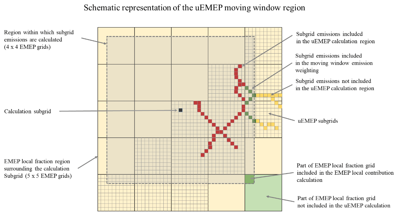
Figure 1Schematic representation of the moving window region. It shows the regions used for uEMEP calculations and the area and emission weighting selection used to determine the local and non-local EMEP contributions at the calculation (receptor) subgrid. The extent of the subgrids is only partially shown.
When the moving window only covers a limited number of EMEP grids and when high-resolution emission data are used that are compatible with the EMEP grid emissions, this weighting can also be based on the high-resolution emission data. This better represents the moving window concept because it reflects the effect of moving the EMEP grid to be centred on the receptor subgrid in a more realistic way. In this case, the emission weighting term (we) on the edge of the moving window will be determined by the fraction of the total subgrid emissions within the moving window and within the EMEP grid, instead of the area. This can be written as
where the numerator is the sum of the emissions within the intersection of a(i,j) and and the denominator is the sum of the emissions within . The resulting total concentration, using this method, may be higher or lower than the original EMEP concentrations because it reflects the impact of moving the EMEP grid in space. This is easiest to visualise if the moving window is the same size as the EMEP grid. If the moving window was centred on an area with concentrated emissions, that are in reality spread over two EMEP grids, then when using the emission weighting the new EMEP local contribution would be higher, the non-local lower and the total would be different; see Fig. 2. The opposite is also true if the moving window were placed over a region with low emissions, the local contribution would be lower and the non-local higher. Due to this, it is not possible simply to subtract the local EMEP contribution from the total to get the non-local EMEP contribution, as detailed in Eq. (5).
To address this, the non-local EMEP contribution is also calculated using the moving window with Eq. (9). The first term is the non-local contribution for a particular source and is calculated with the area weighting distribution since non-local contributions, those outside the local fraction region, do not have any associated emission or local fraction for weighting. An additional correction term, second term in Eq. (9), accounts for the non-local contributions from local contributions on the EMEP edge grids, those parts of the EMEP grids that are outside the moving window and not included as a local contribution in Eq. (6). In those cases, the local EMEP contribution outside the moving window must be converted to a non-local contribution and subtracted from the calculated non-local value (first term in Eq. 9).
In Eq. (9), the weighting term w represents either the emission (we) or the area (wa) weighting, depending on the choice of weighting method.
These local and non-local calculations are carried out for each emission source individually so the non-local contribution is also dependent on source and the non-local component for any particular source will also contain the local contributions from the other sources. This makes creating a final non-local contribution complicated. To solve this, all the source specific contributions are averaged and the sum of the CG,local source contributions are subtracted to obtain the final CG,nonlocal. The final non-local contribution at each subgrid CSG,nonlocal (Eq. 1) is equivalent to the EMEP non-local CG,nonlocal contribution and is calculated by
In the case of area weighting, where the sum of local and non-local contribution is the same as the original EMEP total concentration, then the first term in the summation is equivalent to the original EMEP concentration without summation. The method is illustrated in one dimension in Fig. 2.
The calculation based on emission weighting is computationally more expensive than the area weighting and is only used when necessary and appropriate, e.g. when nmw=1 and when subgrid and grid emissions are consistent with each other.
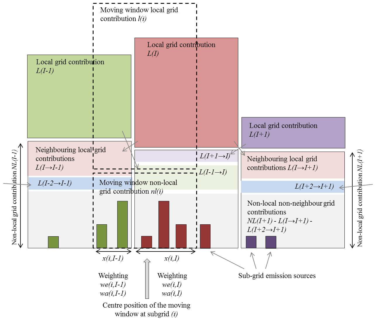
Figure 2Illustration of the moving window interpolation method employed in uEMEP. Shown is the 1-D visualisation of the 2-D method described in Eqs. (6)–(10) for nmw=1. For clarity, in the figure, the terms CG,local and CG,nonlocal are written as L and NL, respectively.
In this section, uEMEP process parameterisations are described. In regard to the dispersion modelling, uEMEP is intended to integrate closely with EMEP. To enable this, dispersion schemes based on parameterisations used in EMEP have been implemented. In the Supplement, additional equations (Sects. S1–S3) are provided and a number of optional additional parameterisations are also described (Sect. S4).
3.1 Subgrid Gaussian dispersion modelling for hourly calculations
A standard Gaussian narrow plume dispersion model formulation, e.g. Seinfeld and Pandis (1998), is used in the subgrid dispersion calculations with multiple reflections from the surface (z=0) and boundary layer height (z=H). Generically, the Gaussian plume calculation can be written as
where for the sake of clarity we have dropped references to subgrid indexes as given in Sect. 2 and use coordinates instead of indices. Here, C is the concentration, Q is the emission source strength and I is the plume intensity given by
Here, hi represents the plume emission height and five additional virtual plume emission heights after single and double reflections from the surface and boundary layer top (H) given by
For the well-mixed plume case, when σz is of the order of H, we define a threshold beyond which the plume concentration is constant throughout the boundary layer. This is specified to occur when σz>0.9H, leading to an intensity given by
The Gaussian dispersion parameters (σz and σy) used in Eq. (12) may be determined empirically (Smith, 1973; Martin, 1976; Turner, 1994; Liu et al., 2015) or through a range of methods based on theoretical and semi-empirical considerations (Seinfeld and Pandis, 1998). Venkatram (1996) also discusses the relationship between empirically and theoretically based dispersion parameters. Standard Gaussian plume models do not take into account variable vertical profiles of wind speed or diffusivity. Some non-Gaussian descriptions are available based on the application of power laws to these profiles and the vertical integration of the diffusion equation (Chaudhry and Meroney, 1973; van Ulden, 1978; Venkatram et al., 2013) but this then creates the problem of defining power laws that “fit” varying wind and dispersion profiles over the entire boundary layer. Instead of this, we use the centre of mass of the plume (zcm) to define the height at which the advective wind speed and eddy diffusivity (Kz) are defined and allow this to vary dependent on the plume travel distance, giving a similar effect to the plume dispersion as the non-Gaussian vertically integrated derivation. A similar methodology is employed by the OPS model (Sauter et al., 2018). We then use a combination of eddy diffusivity (Kz) vertical profiles, Lagrangian timescales and centre of mass plume placement, along with initial values σz0 and σy0, to determine σz and σy values. The aim of this combination is to provide realistic plume dispersion over short distances but to asymptotically approach the same Kz values used in the EMEP model dispersion scheme over longer distances. In addition, the methodology is implementable at all emission heights and takes into account both surface roughness and atmospheric boundary layer height.
Following the methodologies outlined in Seinfeld and Pandis (1998), we describe the dispersion parameters σz and σy as a function of pollutant travel time from source (t) using
where σz0 and σy0 are initial dispersion parameters, Kz(z) and Ky(z) are the vertical profiles of vertical and horizontal eddy diffusivity, and ft is a factor dependent on the Lagrangian integral timescale τl given by
There are many varying methods for calculating the Lagrangian integral timescale (Seinfeld and Pandis, 1998; Hanna, 1981; Venkatram, 1984). We use the formulation from Hanna (1981):
where zemis is the emission height, u∗ is the friction velocity, and m. Time is calculated from the advective velocity:
where xmin is half a subgrid, U(z) is the vertical wind speed profile, and x is the down-plume distance.
In order to be compatible with the EMEP model, the same Kz vertical profile parameterisation is used in Eq. (15a) that is used in EMEP (Simpson et al., 2012). This parameterisation is provided in the Supplement (Eqs. S1–S2).
The centre of mass of the plume is calculated using the same Gaussian formulation with reflection as given in Eq. (12) by integrating the plume intensity over the boundary layer height (H) using
This integral can be analytically solved to give
and for the well-mixed case where
The vertical wind profile is calculated in a similar way to Gryning et al. (2007) based on decreasing turbulent shear with height.
The stability functions (ψm and ϕm) are defined in Eqs. (S3)–(S4) in the Supplement, and the assumptions behind the wind profile derivation are given in Eqs. (S5)–(S8). There is no turning of the wind direction with height. Equation (22) is used to derive u∗0, based on modelled 10 m wind speed, boundary layer height H, Monin–Obukhov length (L) and surface roughness length z0. The vertical wind profile is then derived from this. A minimum wind speed of 0.5 m s−1 for all dispersion calculations has been imposed.
The average of the plume centre of mass height at the receptor point and the emission height, , is then used to determine the vertical diffusion Kz(zav) as well as the wind speed U(zav) for use in Eqs. (15) and (19). The entire set of equations (Eqs. 15–22) is solved iteratively to obtain the final σz value at the receptor point. This iteration converges swiftly and generally only two iterations are required.
The horizontal eddy diffusivity Ky is not determined in EMEP so an alternative is required. Ky can be classically related to Kz through the relationship
based on the concepts used to define K (Seinfeld and Pandis, 1998). Garratt (1994) provides expressions for the vertical profile σv and σw under unstable conditions where the ratio σv∕σw is around 1.85 in the surface layer but decreases to 1 in the mixed layer. Under stable conditions, Nieuwstadt (1984) provides local scaling where this ratio is close to 2. For the current application, we choose the ratio and apply it over the whole boundary layer.
It is also possible within the modelling setup to use the simpler empirical formulations of σz and σy, as presented in Eq. (24) and shown in Table 1. This is useful for testing and comparison, and necessary when using the rotationally symmetric plume parameterisation, Sect. 3.2. See Seinfeld and Pandis (1998) for a presentation of these.
In Fig. 3, we show two example sets of σz curves for near-surface (1 m) and elevated (50 m) releases as calculated with the Kz methodology for three separate stabilities. For reference, the dispersion curves from ASME (American Society of Mechanical Engineers; Smith, 1973) are also shown. These often-used dispersion parameters are relevant for 1 h averaging times. The ASME σz curves are given in Pasquill stability classes and the conversion from their dependency on L and z0 is achieved using the conversion methodology described by Golder (1972). Parameters used in the calculation of the three curves are provided in Table 1.
In addition to the parameterisations presented here, uEMEP also includes parameterisations, provided in the Supplement, for plume meandering and change of wind direction (Sect. S3.4.1), traffic-induced initial dispersion (Sect. S3.4.3) and road tunnel internal deposition and emissions (Sect. S3.4.5).
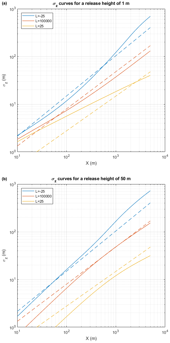
Figure 3Comparison of derived σz curves discussed in the text with standard ASME curves (Smith, 1973) using Eq. (24). To the left is a 1 m release and to the right a 50 m release. Three different stability classes, specified by the Monin–Obukhov lengths (L), are shown. The Kz method is shown as a solid line and the ASME curves as dashed lines. The ASME curves have no release height or surface roughness dependence but are included as reference. Values of z0=0.5 m, relevant for urban areas, and σz0=0 are used.
Table 1Parameters used for calculating the curves shown in Fig. 3.

3.2 Rotationally symmetric Gaussian plume model for annual mean calculations
When applying uEMEP to annual mean emissions, a rotationally symmetric Gaussian plume is used. It is possible to derive an approximate analytical solution to the Gaussian plume equation assuming that wind directions are homogeneously distributed in all directions and that there is no strong dependence of wind speed or stability on wind direction. These conditions are usually not met but it is useful to have such a simplified analytical solution.
The starting point is the Gaussian plume model given in Eq. (12). In this case, we do not derive σy,z using the Kzvalue from EMEP but apply the commonly used power law formulation in order to derive an analytical solution:
Values for the dispersion parameters a and b may be taken from the literature (Seinfeld and Pandis, 1998) but we use the ASME curves (Smith, 1973) under neutral conditions to specify these.
The rotationally symmetric version of this equation can be derived by rewriting the equation in cylindrical coordinates with appropriate approximations (second order), based on the slender plume assumption, and integrating over all angles. The resulting rotationally symmetric intensity Irot(r,z) as a function of r and z is then written
where
The term B can be less than −1, typically when , which can lead to imaginary solutions. This is due to the second-order approximation made in converting to cylindrical coordinates. In that case, we write a second-order approximation based on Taylor series expansion around as
A similar derivation has been carried out by Green (1980) using different assumptions for the form of Eq. (24).
3.3 Initial dispersion
In Sect. 3.1 and 3.2, the hourly and annual dispersion parameterisations are described. In both cases, initial values for σ0(y,z) are required. Since we treat the sources as small area emitters, we set the initial σ0y to correspond to these areas. A value of will give a maximum subgrid centre concentration equivalent to the concentration that would be found if the emissions were distributed evenly in the subgrid. We then write the total initial dispersion to be
In all applications of uEMEP, Δx=Δy. The other parameter, σinit,y, is a specific initial dispersion width for each individual emission source, for example, 2 m for traffic and 5 m for shipping, heating and industry. This is generally much smaller than the emissions grids.
The initial value for σ0z is also a combination of a specific emission initial dispersion, for example, m for residential wood combustion but also uses the displacement technique for the plume where the start of the plume is displaced upwind by Δx∕2 allowing the plume to grow vertically over half the subgrid distance. Tunnel exits are given an initial m to represent the extended size of the tunnel portals.
3.4 NO2 chemistry for hourly means
The only chemistry included in uEMEP is the NOx, O3 chemical reactions. We use a similar methodology to Benson (1984, 1992) known as the discrete parcel method but use a weighted timescale over which the reactions take place. The following chemical reactions are involved, with Ox (O3+NO2) and NOx (NO+NO2) concentrations being conserved:
Equation (29c) occurs on timescales much faster than the two other reactions and is taken to be instantaneous. The differential equation for the concentration of [NO2] as a function of time is written as
where the concentrations are expressed in terms of molecules per cm3 and J is the photolysis rate (s−1) for Eq. (29b) taken from the EMEP model (Simpson et al., 2012). The reaction rate k1 for Eq. (29a) is given by
as in the EMEP model and where Tair is in the atmospheric temperature (K).
We rewrite Eq. (30) in terms of the dimensionless ratios:
Equation (30) then becomes
The solution to this equation is
where
and is the initial NO2 fraction at time .
This solution is valid for a box model without dilution through dispersion since it does not take into account how changing NOx and Ox concentrations over the plume travel time will affect the reaction rates. Though this could be accounted for when applied to a single source with assumed dilution rates, by adding a time-dependent diluting term to Eq. (30), this is not practically possible for multiple sources of differing dilutions. The concentrations of NO2 at the start of the plume will be correctly calculated but NO2 concentrations further from the plume will be slightly underestimated, since they do not have the higher initial reaction rates. Eventually, the concentrations will reach photostationary equilibrium and here too NO2 will be correctly calculated. This special case for photostationary equilibrium in Eq. (35) occurs when and Eq. (34) becomes
The non-linear nature of Eq. (34) also means that it cannot be consistently applied to Gaussian models since the shape of the plume will change due to the non-linearity. Despite this, this formulation is more physically realistic than the photostationary assumption often used in local-scale air quality modelling or other less physical parameterisations based on empirical fits. See Denby (2011) for an overview of the various NO2 chemistry parameterisation methods used with Gaussian modelling. In order to calculate Eq. (34) in the model application, an initial NOx and Ox concentration must be used and a travel time defined. For multiple sources, this travel time will vary so for each calculated subgrid concentration of NOx from each contributing subgrid source (ns sources) a travel time, ts, is calculated based on the distance and wind speed. This is weighted based on the contribution of each source to the total subgrid NOx concentration. This provides a final weighted travel time tw that is applied in Eq. (34). This ensures that the nearest of the contributing subgrids, often with the highest contributing NOx concentrations, are given a higher travel time weight. A minimum distance, and hence time, of half a subgrid is applied when calculating travel times.
Comparisons with EMEP NO2 calculations show that this chemistry scheme matches the results obtained by EMEP over longer time periods.
3.5 NO2–NOx conversion for annual means
When annual mean data are used, the hourly mean formulation cannot be applied. Instead, we use an empirically based conversion of NOx to NO2 based on the type of formulation from Romberg (1996) and updated by Bächlin and Bösinger (2008). A total of 3 years of Norwegian NO2 measurements, 82 measurements in all, have been used to determine this relationship (Fig. 4).
The fitted constants are determined to be a=20, b=30, and c=0.23. The estimated uncertainty in this conversion is around 10 %, based on the normalised root mean square error of the fitted and observed NO2 concentrations.
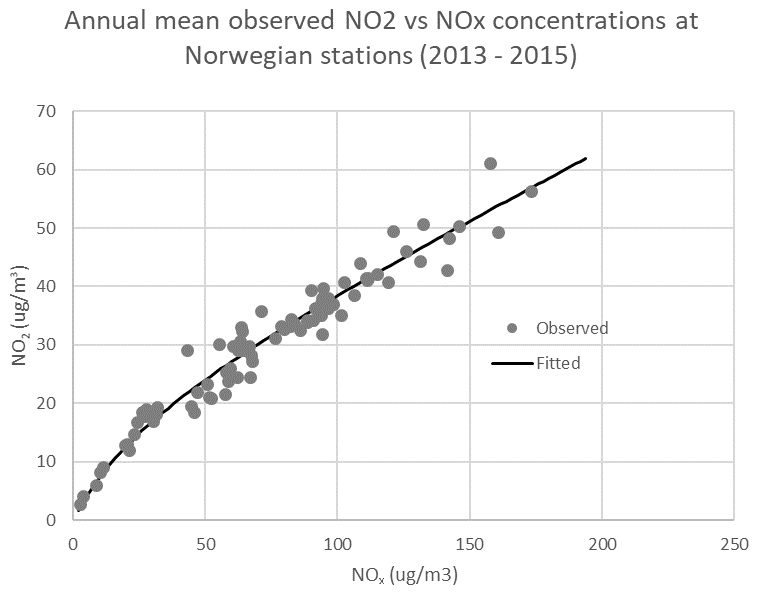
Figure 4NO2 versus NOx annual mean concentrations for all stations in Norway in the period 2013–2015. The fitted curve is based on Eq. (38).
This empirical relationship will vary from region to region, largely due to differences in O3 concentrations and photolysis rates that are not included as part of the parameterisation. If used over large regions, for example, Europe, then the uncertainty in the NO2 conversion will increase.
3.6 Implementation
3.6.1 Subgrid domains
Within uEMEP, individual domains are defined with differing resolutions and sizes, dependent on which modelling parameter is represented. Separate domains and subgrid resolutions are defined for each of the emission sources, for the time profiles of each emission source, for the meteorological data, for the population data and for the receptor subgrid concentrations. None of these are required to have the same resolution or size; however, the highest-resolution emission subgrid will define the receptor subgrid resolution, since there is no need to calculate on higher-resolution subgrids than is provided by the emissions. For emission subgrids with lower resolution than the final receptor subgrid domain, the dispersion calculations are first carried out at the same resolution as the emission domain and then bilinearly interpolated to the receptor subgrid. For most urban applications, this means that the choice of traffic subgrid resolution defines the highest-resolution subgrid.
Emission subgrids also contain properties for the dispersion calculations, such as initial dispersion parameters and emission heights. Each emission subgrid has only one emission height hemis, one σinit,z0 and one σinit,y0 for each emission source type. When multiple emissions from the same source type are placed in an emission subgrid, the emission parameters are weighted by each individual emission. This is most relevant for industrial emissions which may have different emission heights from separate stacks within a single emission subgrid.
3.6.2 Selective subgrid calculations
uEMEP does not necessarily calculate concentrations at all receptor subgrids. Only subgrids which are within 3σy of a plume centre line will be calculated and also downwind selection is used (Sect. S3.4.2 in the Supplement). In addition, a number of selections can be made, allowing quicker calculations for particular applications. These include the following:
-
For calculation at defined receptor points, usually corresponding to measurement stations, uEMEP calculates the surrounding nine subgrids and uses bilinear interpolation to extract the concentrations at the required receptor position.
-
For calculation at population grids, concentrations will only be calculated at grids with non-zero population. This provides quicker exposure calculations than if the entire region was calculated.
-
A routine for selecting a higher density of subgrids near sources may also be used to speed up calculations. This applies most often to traffic emission subgrids that are near the surface and with large gradients near the source. This is less useful for higher release sources as their maximum impact occurs further downwind than their emissions. After calculation, the lower-density receptor subgrids are interpolated into the rest of the receptor subgrids, providing a full receptor subgrid domain.
3.6.3 Model inputs and outputs
Input data come from a variety of sources and the formatting of these sources varies. Emission input data are generally in text format whilst meteorological files are read from NetCDF files.
Output of the model is in the form of NetCDF files for either gridded data or point data, if receptor points have been defined. In both of these files, output includes the total concentrations of the pollutants along with the source contribution from each of the emission sources used in the calculation. Speciation of PM from EMEP can also be included in the output files, along with emissions, meteorology and population data.
Though uEMEP has been applied in a number of applications we select the Norwegian forecast and analysis system (Norwegian air quality forecasting service, 2020) as an example. This application started operationally in the winter of 2018–2019 and provides daily forecasts of air quality for all of Norway 2 d in advance at subgrid resolutions of between 250 and 50 m. In addition, the same system is used to calculate air quality retrospectively for analysis and planning applications (Norwegian air quality expert user service, 2020). The compounds PM2.5, PM10, NO2, NOx and O3 are calculated. For each of these, the local source contributions are determined separately for traffic exhaust, traffic non-exhaust, residential wood combustion, shipping and industry. A cascade of models is used, starting with EMEP MSC-W at 0.1∘ European domain, EMEP MSC-W at 2.5 km Scandinavian domain and uEMEP 250–50 m Norway only (Fig. 5).
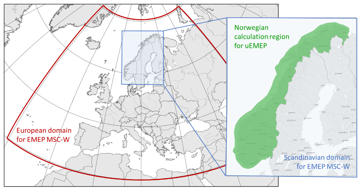
Figure 5Model domain for the European and Scandinavian EMEP MSC-W calculations and the uEMEP calculations (© kartverket/norgeskart.no).
4.1 Calculation steps
We describe below the implementation steps used in the Norwegian forecasting and analysis system. This implementation of uEMEP uses the independent emission and replacement downscaling method (method 2 in Sect. 2). The following steps are carried out:
- 1.
High-resolution emission data for Norway are calculated for each forecast (Sect. 4.2) and are aggregated into the EMEP MSC-W Scandinavian model grid. Some of these emissions require meteorological data.
- 2.
The EMEP MSC-W model is used to calculate the large-scale concentration distribution on an hourly basis, nesting from a European domain (∼ 0.1∘) to the Scandinavian domain (2.5 km) (Fig. 5). Within Norway, the aggregated high-resolution aggregated emissions are implemented. Both EMEP calculations provide the local fraction (Sect. 2.3) in a region of 5×5 EMEP grids.
The following three steps are then undertaken to calculate the uEMEP concentrations:
- 3.
For the Norwegian forecast system, the entire country is split into 1864 separate tiles of varying sizes and resolutions, with the resolution depending on the population and emission sources within each tile. Tiles with resolutions of 250 m can be as large as 40×40 km2, whilst tiles with resolutions of 50 m are no larger than 5×5 km2. Tiling the calculations is a form of external parallelisation and is optimised for both runtime and memory use. A 2 d forecast run on 196 processors takes roughly 1 h of CPU time.
- 4.
The high-resolution emission data from the various source sectors (Sect. 4.2) are placed into the emission subgrids in uEMEP. These are between 50–250 m in width, depending on the emissions available and on the population density of the region. Emission grid domains extend beyond the size of each tile so that the calculations are consistent over tile borders.
- 5.
uEMEP Gaussian dispersion modelling is applied (Sect. 3.1) using the subgrid emissions as sources and the concentrations are calculated at each subgrid. Only subgrid emissions within a region defined by a 4×4 EMEP grid area are included in the subgrid calculation, i.e. 10×10 km2, corresponding to the extent of the moving window. This 4×4 limit guarantees that the calculation will always be carried out within the EMEP 5×5 local fraction region.
The final steps combine the EMEP gridded concentrations with the uEMEP subgrid concentrations in the following way:
- 6.
At each subgrid, the non-local contribution from the neighbouring 4×4 EMEP grids is calculated (Sect. 2.4). The calculation is carried out for each source sector and each primary compound.
- 7.
The uEMEP calculations are then added to the non-local EMEP concentrations. In the case of PM, all non-primary species are also added to the local and non-local EMEP primary concentrations.
- 8.
For NO2, the chemistry (Sect. 3.4) is applied to determine NO2 and ozone for each subgrid.
- 9.
Subgrid concentrations and their contributions are saved along with the PM speciation from EMEP in NetCDF format.
- 10.
The forecasts are made available to a public website through an API and Web Map Tile Server (Norwegian air quality forecasting service, 2020).
The system is schematically illustrated in Fig. 6. The following sections describe some steps in more detail.
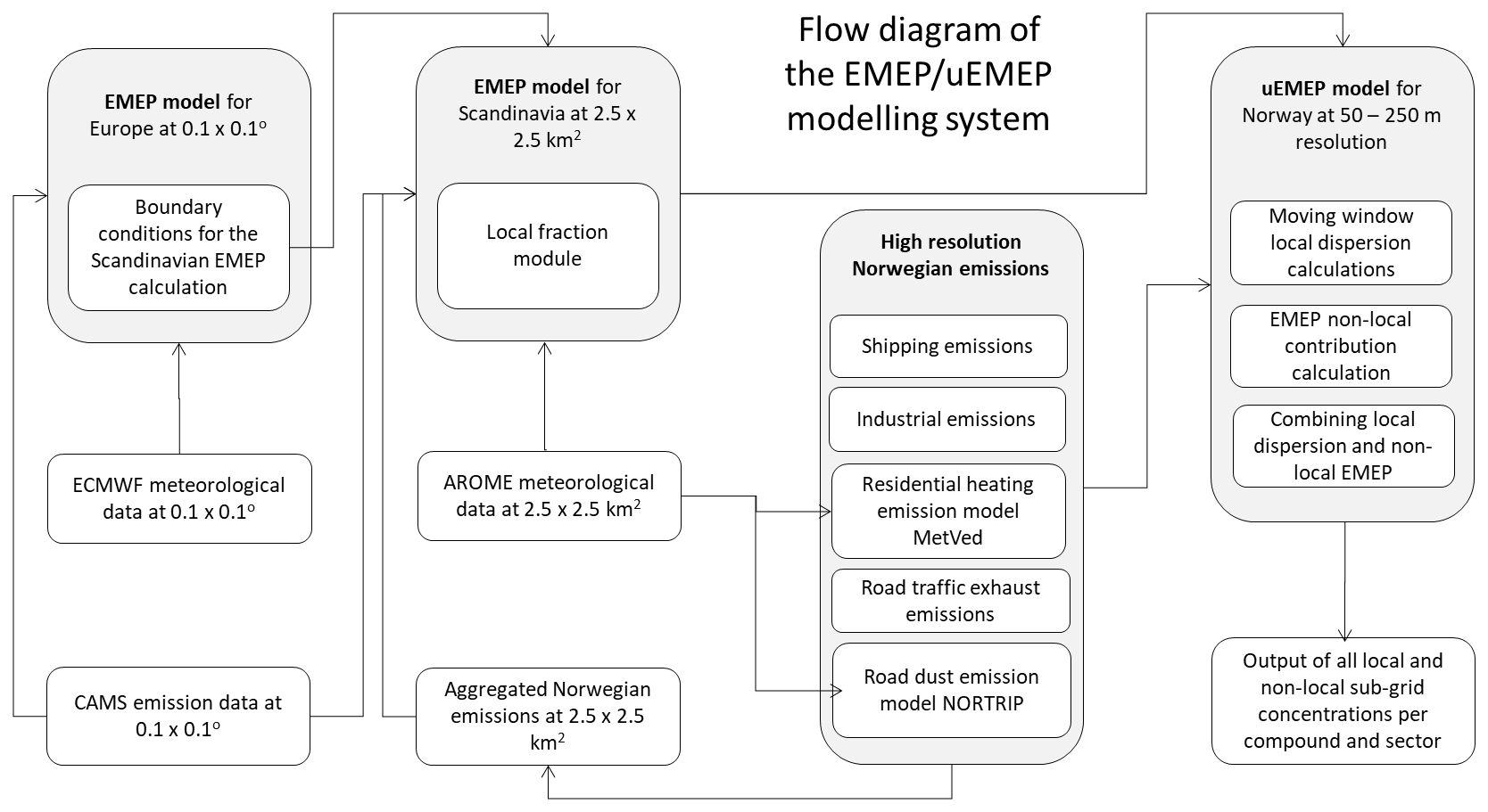
Figure 6Flow diagram showing the various components of the Norwegian EMEP/uEMEP forecast system.
4.2 Emissions
The EMEP calculations make use of the CAMS-REG-AP_v1.1 regional anthropogenic emission dataset everywhere in Europe (Kuenen et al., 2014; Granier et al., 2019). Only in the 2.5 km Scandinavian calculation, and only in Norway, are the emissions replaced with the aggregated high-resolution dataset. The alternative emissions used in the calculations for Norway are
-
road traffic exhaust emissions,
-
road traffic non-exhaust emissions,
-
residential wood combustion,
-
shipping and
-
industry.
These emission sources are described in Sect. S4.2 in the Supplement. For other sectors, the CAMS-REG-AP_v1.1 emissions are also used in Norway, but these emissions are not downscaled using uEMEP.
4.3 Meteorology
The meteorological forecast data used for the European EMEP model calculations are based on the Integrated Forecasting System (IFS, 2020) from the European Centre for Medium-Range Weather Forecasts (ECMWF, 2020). The Scandinavian EMEP model calculation uses the AROME-MetCoOp model for modelling meteorology over Scandinavia (Müller et al., 2017). This last model calculates meteorology at a resolution of 2.5 km and provides forecasts for 66 h in advance. The EMEP MSC-W Scandinavian domain uses the same gridding and projection as the meteorological forecast model but in a smaller domain.
4.4 EMEP MSC-W model implementation
The European EMEP MSC-W model calculation is based on the same daily forecast provided for the Copernicus Atmosphere Monitoring Service (CAMS, 2020; Tarrason et al., 2018) but is run independently and provides boundary conditions for the Scandinavian implementation of EMEP MSC-W at 2.5 km. The Scandinavian EMEP MSC-W calculation includes the Norwegian emission sources described in Sect. 4.2 and also delivers the necessary local fraction information for use in uEMEP.
4.5 uEMEP model implementation
uEMEP calculates concentrations for all of Norway on grids with resolutions between 50 and 250 m using 1864 individual tiles as described in Sect. 4.1. The resolution of these tiles is defined by the population density and road density information. Tiles with higher population density use 50 m resolution, whilst tiles with lower population density but some traffic have a resolution of 125 m. Tiles with very low traffic density but with shipping or wood burning emissions have a resolution of 250 m, corresponding to the emission resolution. Separate calculations are carried out at measurement sites, 72, with a subgrid resolution of 25 m. An example of a PM10 forecast is shown in Fig. 7.
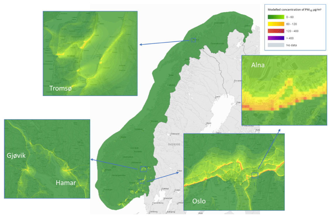
Figure 7Example maps of PM10 concentrations taken from the forecast on 24 February 2020 at 18:00 UTC. The resolution in populated city regions is 50 m. High PM10 concentrations along roads are mainly the result of road dust emissions (© kartverket/norgeskart.no).
5.1 Validation against observations for the Norwegian forecasting and assessment system
Here, we present a visual summary of results for NO2, PM10 and PM2.5 for the year 2017, when there were 72 operational air quality stations. Not all stations measure all components so the total number of available stations for NO2 and PM with coverage of more than 75 % is between 34 and 45. The station positions are shown in Fig. 8.
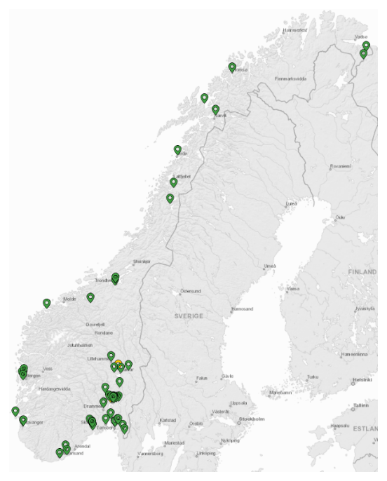
Figure 8Positions of all 72 monitoring stations in Norway: 33 for PM2.5, 36 for NO2, 45 for PM10 and 8 for O3 (© kartverket/norgeskart.no).
Figure 9 shows the comparison of modelled and observed NO2 for annual average at each station (scatter plot) and daily mean temporal profile averaged over all stations. Included in the scatter plot are the Scandinavian EMEP MSC-W results at 2.5 km. The spatial correlation is quite high, r2=0.81 for uEMEP with little negative bias (FB of −5.9 %). The temporal variation over the whole year is also well represented when averaged over all stations (r2=0.79).
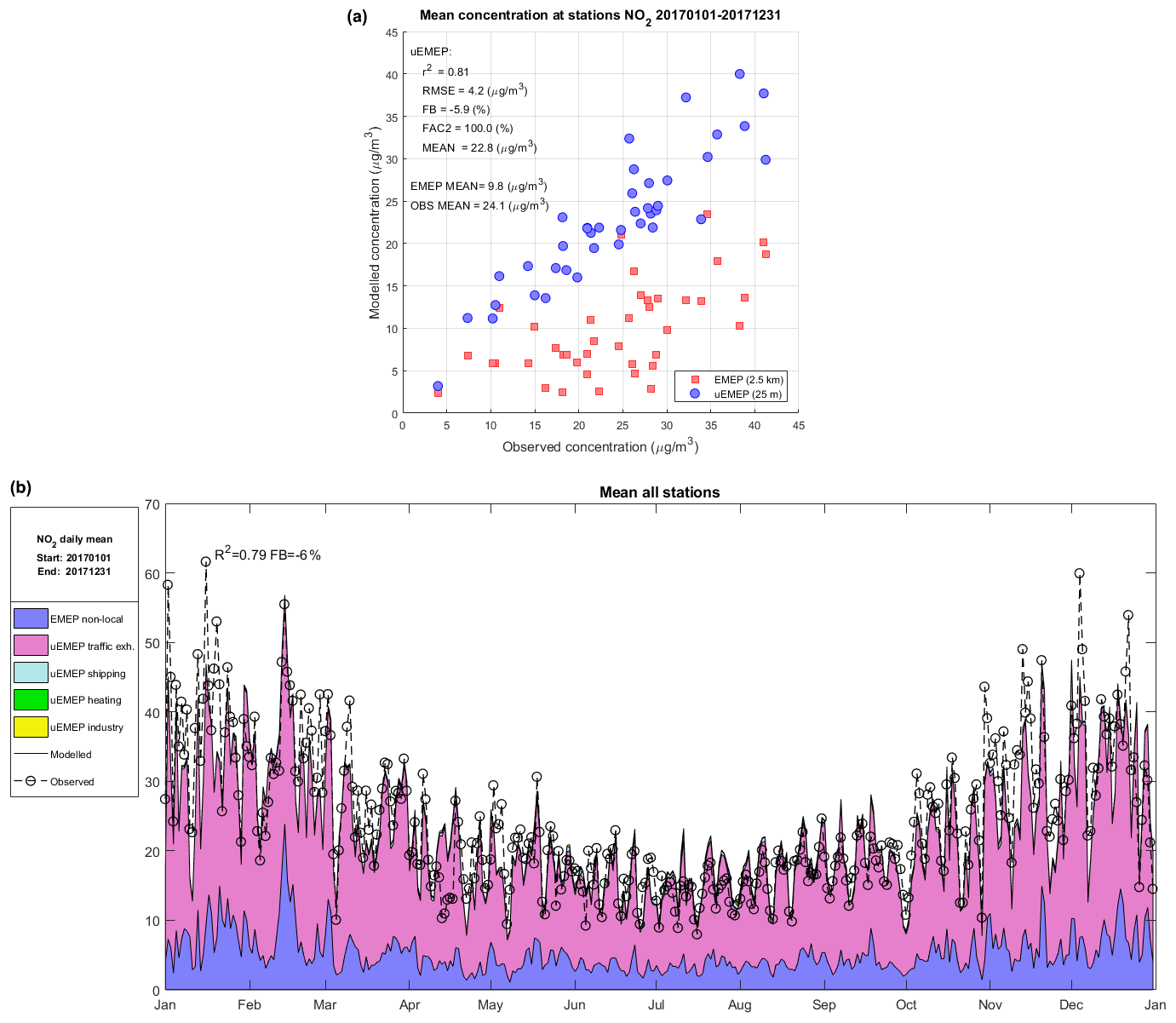
Figure 9(a) Scatter plot comparison of modelled and observed NO2 for annual average concentrations at each station. Shown are the results for both uEMEP and EMEP. Comparative statistics are shown for the uEMEP calculation. EMEP and observed means are also included. (b) Daily mean temporal profile averaged over all stations. Source contributions are shown for the temporal modelling results along with the EMEP 2.5 km calculation (EMEP4NO). In total, 36 stations are used in the comparison.
Figure 10 shows the comparison of modelled and observed PM10 for annual average at each station (scatter plot) and daily mean temporal profile averaged over all stations. Included in the scatter plot are the Scandinavian EMEP results at 2.5 km. The spatial correlation is low, r2=0.29 for uEMEP with little negative bias (FB of −9.2 %). The temporal variation over the whole year is well represented when averaged over all stations (r2=0.61) but the model has a negative bias of 4 µg m3 over much of the summer period. Road dust events in the springtime are well captured by the NORTRIP emission model.
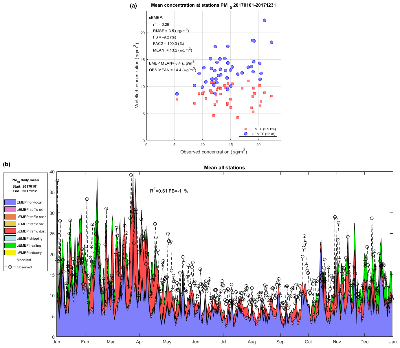
Figure 10(a) Scatter plot comparison of modelled and observed PM10 for annual average concentrations at each station. Shown are the results for both uEMEP and EMEP. Comparative statistics are shown for the uEMEP calculation. EMEP and observed means are also included. (b) Source contributions from both uEMEP and EMEP models are shown for the temporal modelling results along with the EMEP 2.5 km calculation (EMEP4NO). A total of 45 stations are used in the comparison.
Figure 11 shows the comparison of modelled and observed PM2.5 for annual average at each station (scatter plot) and daily mean temporal profile averaged over all stations. Included in the scatter plot are the Scandinavian EMEP results at 2.5 km. The spatial correlation is good, r2=0.49 for uEMEP with little negative bias (FB %). The temporal variation over the whole year is well represented when averaged over all stations (r2=0.67) but the model has a negative bias of 2 µg m3 over much of the summer period. Residential wood combustion (heating) events in the winter are well captured by the emission model MetVed.

Figure 11(a) Scatter plot comparison of modelled and observed PM2.5 for annual average concentrations at each station. Shown are the results for both uEMEP and EMEP. Comparative statistics are shown for the uEMEP calculation. EMEP and observed means are also included. (b) Source contributions are shown from both uEMEP and EMEP models for the temporal modelling results along with the EMEP 2.5 km calculation (EMEP4NO). A total of 33 stations are used in the comparison.
5.2 Verification and sensitivity tests
In addition to the validation against monitoring data, a number of verification and sensitivity experiments have been undertaken with the model. These include
-
comparison of single annual mean calculations with the mean of hourly calculations,
-
sensitivity to the moving window size,
-
sensitivity to the choice of resolution,
-
sensitivity to the temperature dependence of NOx exhaust emissions and
-
sensitivity to the choice NO2 ∕ NOx initial exhaust ratio.
These sensitivity tests are provided in the Supplement (Sect. S5). We present only conclusions from these.
5.2.1 Comparison of single annual mean calculations with the mean of hourly calculations
In Sect. 3, we describe two methods for calculating dispersion. One is based on the hourly meteorological and emission data (Sect. 3.1) and the other on annual mean data (Sect. 3.2). A rotationally symmetric dispersion kernel (Eq. 25) is used for dispersion of the annual mean emissions. Tests using the same dispersion parameters in both annual and hourly calculations (Sect. S5.1) give very similar results for both methodologies indicating the validity of the annual mean calculation. When Kz-based dispersion (Eqs. 15–23) is used in the hourly calculations, there is a larger difference between the two methods because of the difference between the two dispersion parameterisations. We conclude that the time-saving advantage of the single annual mean calculation, approximately 10 000 times faster, and the similarity to the hourly calculation make it an efficient and valid method for calculating high-resolution annual maps of air quality.
5.2.2 Sensitivity to the moving window size
The size of the moving window region within which uEMEP calculates local high-resolution concentrations should impact on the results since smaller moving windows will include less locally modelled contributions and more non-local EMEP contributions. This has been verified in a sensitivity study, (see Sect. S5.2 in the Supplement). In this sensitivity experiment, the moving window size was varied from nmw=1 to eight EMEP grids, and calculations were made at existing measurement sites. The mean concentrations are shown to be quite insensitive to the choice of this region, particularly for PM10. Generally, the reduction in the local contribution is well balanced with the increase in the non-local contribution when reducing the size of the moving window, verifying the methodology. It is recommended to use a minimum of two EMEP grids for the moving window region.
5.2.3 Sensitivity to the choice of resolution
The choice of subgrid resolution will impact on the calculated concentrations, both in concentration levels and in spatial distribution. An experiment where a range of subgrid resolutions were tested, from 15 to 250 m, was carried out (Sect. S5.3). Calculations were made at the positions of the Norwegian monitoring sites, most of which are traffic sites. The results showed that even at resolutions of 250 m the mean concentrations for all stations were very similar. At 100 m resolution, compared to the reference of 25 m, the difference in annual mean was no larger than 15 % at any one station with a normalised root mean square error (NRMSE) of 6 %. The NRMSE increased to 11 % for the 250 m calculation with a maximum deviation of 40 % at one station. We conclude that 100 m resolution will provide good concentration estimates for near-road calculations though higher resolutions may be required, depending on the application.
5.2.4 Sensitivity to the temperature dependence of NOx exhaust emissions
The temperature dependence of the NOx traffic exhaust emissions was assessed by running the model with and without this dependency (Sect. S5.4). With this correction, the results show a significant improvement in the station mean time series correlation (from r2=0.68 to 0.79) and improved correlation in both the daily (from r2=0.56 to 0.60) and annual (from r2=0.76 to 0.78) mean calculations. Bias is also reduced from −20 % to −3 %. The correction factor used (Eq. S13) still requires further evaluation and should be considered only as an initial estimate.
5.2.5 Sensitivity to the choice NO2 ∕ NOx initial exhaust ratio
In the calculations shown in Fig. 9 for NO2, an initial NO2 ∕ NOx exhaust emission ratio of 0.25 was used. This reflects the large portion of diesel vehicles used in Norway and the high NO2 ∕ NOx ratio of these (Hagman et al., 2011). However, comparison of modelled ratios of NO2 ∕ NOx indicate this ratio may be too high. This was assessed by running the model with three different ratios: 0.15, 0.25 and 0.35. The results (Sect. S5.5) show that an NO2 ∕ NOx ratio of 0.15 most closely fits the observed ratio and this ratio will be implemented in further applications of the model.
The aim of uEMEP is to provide downscaling capabilities for the EMEP MSC-W model with the intention of improving exposure estimates and more realistic concentrations at high resolution over large areas. The example application provided, the Norwegian air quality forecast and expert user service, is an example of how high-resolution coverage over large regions (countries) can be achieved. The validation carried out in Sect. 5.1 shows that the modelling system provides moderate to good comparison with observations. The best results are for NO2, chiefly because we have the best information concerning emissions that contribute to these concentrations, i.e. traffic exhaust. The lower correlation of PM is indicative of the difficulties in modelling emissions such as residential wood burning and road dust emissions. That NO2 is well modelled indicates that the problems lie largely with the emissions rather than the dispersion model itself. In addition, a large proportion of PM is due to medium to long-range transport and secondary formation of particles. This is not part of the uEMEP model but relies on the EMEP MSC-W model and the emissions included there.
The strength of the modelling system is in the integration of uEMEP with EMEP through the use of the local fraction. This allows downscaling anywhere within an EMEP domain provided that suitable proxy data are available for the downscaling. This is an important aspect of the modelling and is the link that can bind the regional- and local-scale emission communities. Usually the proxies used for regional-scale emission inventories are not available to the user so that exactly how these emissions are made, quantitatively, is unknown to the user. In addition, as the resolution of regional-scale emission inventories increases, so too does the need for improved spatial distribution proxies. Population density, successfully used to distribute a range of emission sectors on low-resolution grids (> 10 km), is no longer suitable for many sectors since at high resolution the emissions are no longer correlated with population. This was discussed in an earlier paper (Denby et al. 2011) and remains problematic.
When implementing uEMEP, it is highly desirable that the emissions used in both uEMEP and EMEP models are consistent with one another. This has been achieved for the Norwegian application for the traffic, domestic heating, shipping and industry sectors. However, other sources, such as other mobile combustion sources associated with construction and other activities, are not included. These can be of importance locally even if they are not significant on the regional scale. There is no clear methodology available on how to implement these emissions at the required resolution.
The modelling system has limitations. Currently, only primary emissions, with the exception of NO2 formation, are dealt with. Some secondary formation of particles will likely occur within the local region used for the uEMEP model domain but these are not currently accounted for. uEMEP is also a Gaussian model that does not take into account obstacles of any type. When achieving resolutions of 50 m, buildings start to play an important role in the transport and dispersion. The region covered by the local-scale modelling, the moving window region, is necessarily limited in extent. Sensitivity studies show that this has limited impact on mean concentrations but for source sectors such as industry, that are released at height, the limited calculation region may not be large enough to include all of the plumes impact region.
In many ways, the increase in resolution to almost street level puts new demands on the modelling system that were not necessary to consider previously. For regional-scale modellers, the downscaling can provide considerable improvement to regional calculations. However, from a local-scale modelling perspective, the local-scale information may not be of sufficient quality to be useful to local users. This is most important when only proxy data are available for downscaling rather than actual bottom up emissions. In the end, if high-resolution modelling is to be used at the local scale, then similar high-quality emission data will be required if the results are to be useful to users.
There are a number of aspects of the modelling system that can be, and are being, improved. These include
-
implementation of dry and wet deposition in uEMEP (currently not included in this version),
-
improving the annual mean dispersion kernel dispersion parameters to be more consistent with the hourly Kz methodology,
-
implementing necessary secondary formation of PM in uEMEP,
-
further assessment of the Kz Gaussian plume methodology and
-
refinement of the temperature dependence of NOx traffic exhaust emissions.
A number of aspects were not treated in this paper but will be topics of further studies. These include population exposure and the impact of resolution, trend assessment in emissions and analysis of road dust emissions for all of Norway. In addition, the modelling system is being applied in a number of different countries and results of these applications will be further described and assessed.
This paper presents and documents a new downscaling model and method (uEMEP) for use in combination with the EMEP MSC-W chemical transport model. Process descriptions and parameterisations within the uEMEP model are provided and the methodology for combining uEMEP with EMEP MSC-W local fraction calculations is elaborated. An example application, the Norwegian air quality forecast system, is presented and validation for the year 2017 at all available Norwegian air quality stations is provided. A number of verification and sensitivity studies are summarised in the paper and expanded in the Supplement.
The uEMEP model provides a new methodology for downscaling regional-scale chemical transport models but can currently only be applied together with the EMEP MSC-W model since this is the only model with the necessary local fraction calculation. The uEMEP model is based on Gaussian modelling that has existed for many years but it does use specific parameterisations to describe the dispersion parameters in order to be compatible with the EMEP model application.
uEMEP can provide improved exposure estimates if suitable proxy data for emissions are available and can be applied to regions as large as the regional-scale CTM in which it is imbedded. It can also represent concentrations down to street level, though not street canyons, and is comparable with traffic monitoring sites. This makes it a unique system for assessment, policy application and forecasting purposes.
The current version of uEMEP is available from GitHub (https://github.com/metno/uEMEP) under the GNU Lesser General Public License v3.0. The code is written in Fortran 90 and is compilable with Intel Fortran (ifort). The code does not support gfort as a compiler at this time. The exact version of the model used to produce the results used in this paper is archived on Zenodo (https://doi.org/10.5281/zenodo.3756008; Denby, 2020a), as are input data and scripts to run the model and produce the plots for all the simulations presented in this paper (https://doi.org/10.5281/zenodo.3755573; Denby, 2020b).
The supplement related to this article is available online at: https://doi.org/10.5194/gmd-13-6303-2020-supplement.
BRD is the lead author of the article and developer of the uEMEP model. MG and HF internally reviewed and contributed to the writing of the article. PW is the developer of the local fraction methodology in the EMEP MSC-W model and provided text on this. QM carried out the EMEP MSC-W calculations for this article and contributed to the text. EGW carried out the validation of the uEMEP model and contributed to the text. AV and HK provided the technical support for carrying out the modelling and contributed to the uEMEP code and associated scripts for its implementation.
The authors declare that they have no conflict of interest.
uEMEP development was supported by the Research Council of Norway (NFR), the Norwegian Public Roads Administration (Statens Vegvesen), the Norwegian Environment Agency (Miljødirektoratet) and the Ministry of Climate and Environment (Klima-og miljødepartementet).
This research has been supported by the Research Council of Norway (NFR) project “AirQuip” (grant no. 267734).
This paper was edited by Augustin Colette and reviewed by two anonymous referees.
Andersson, C., Langner, J., and Bergström, R.: Interannual variation and trends in air pollution over Europe due to climate variability during 1958–2001 simulated with a regional CTM coupled to the ERA40 reanalysis, Tellus, 59B, 77–98, https://doi.org/10.1111/j.1600-0889.2006.00196.x, 2007.
Appel, K. W., Napelenok, S. L., Foley, K. M., Pye, H. O. T., Hogrefe, C., Luecken, D. J., Bash, J. O., Roselle, S. J., Pleim, J. E., Foroutan, H., Hutzell, W. T., Pouliot, G. A., Sarwar, G., Fahey, K. M., Gantt, B., Gilliam, R. C., Heath, N. K., Kang, D., Mathur, R., Schwede, D. B., Spero, T. L., Wong, D. C., and Young, J. O.: Description and evaluation of the Community Multiscale Air Quality (CMAQ) modeling system version 5.1, Geosci. Model Dev., 10, 1703–1732, https://doi.org/10.5194/gmd-10-1703-2017, 2017.
Bächlin, W., Bösinger, R.: Untersuchungen zu Stickstoffdioxid-Konzentrationen, Los 1 Überprüfung der Rombergformel, Ingenieurbüro Lohmeyer GmbH & Co. KG, Karlsruhe, Projekt 60976-04-01, Stand: Dezember 2008, Gutachten im Auftrag von: Landesamt für Natur, Umwelt und Verbraucherschutz Nordrhein–Westfalen, Recklinghausen, 2008.
Benson, P.: A review of the development and application of the CALINE3 and 4 models, Atmos. Environ., 26B:3, 379–390, https://doi.org/10.1016/0957-1272(92)90013-I, 1992.
Benson, P.: CALINE4 – A dispersion model for predicting air pollutant concentrations near roadways, FHWA/CA/TL-84/15, California Department of Transportation, Sacramento, CA, available at: https://ntrl.ntis.gov/NTRL/dashboard/searchResults.xhtml?searchQuery=PB85211498 (last access: 8 December 2020), 1984.
Brandt, J., Christensen, J., Frohn, L., and Zlatev, Z.: Operational air pollution forecast modelling using the THOR system, Phys. Chem. Earth, 26, 117–122, https://doi.org/10.1016/S1464-1909(00)00227-6, 2001.
CAMS: Copernicus Atmosphere Modelling Service (CAMS), Air quality forecasts Europe, available at: https://atmosphere.copernicus.eu/, last access: 8 December 2020.
Chaudhry, F. H. and Meroney, R. H.: Similarity theory of diffusion and the observed vertical spread in the diabatic surface layer, Bound.-Lay. Meteorol., 3, 405–415, https://doi.org/10.1007/BF01034984, 1973
Cimorelli, A. J., Perry, S. G., Venkatram, A., Weil, J. C., Pain, R. J., Wilson, R. B., Lee, R. F., Peters, W. D., Brode, R. W., and Paumier, J. O.: AERMOD: Description of model formulation, EPA-454/R-03-004, available at: http://www3.epa.gov/scram001/7thconf/aermod/aermod_mfd.pdf (last access: 8 December 2020), 2004.
Denby, B., Cassiani, M., de Smet, P., de Leeuw, F., and Horálek, J.: Sub-grid variability and its impact on European wide air quality exposure assessment, Atmos. Environ., 45, 4220–4229, https://doi.org/10.1016/j.atmosenv.2011.05.007, 2011
Denby, B. R.: Guide on modelling Nitrogen Dioxide (NO2) for air quality assessment and planning relevant to the European Air Quality Directive. ETC/ACM Technical paper 2011/15, available at: https://www.eionet.europa.eu/etcs/etc-atni/products/etc-atni-reports/etcacm_tp_2011_15_fairmode_guide_modelling_no2 (last access: 8 December 2020), 2011.
Denby, B. R.: metno/uEMEP: uEMEPv5 (Version 5.0), Zenodo, https://doi.org/10.5281/zenodo.3756008, 2020a.
Denby, B. R.: uEMEP startup configuration and data file for GMD uEMEP model description publication [Data set], Zenodo, https://doi.org/10.5281/zenodo.3755573, 2020b.
ECMWF: ECMWF home page, available at: http://www.ecmwf.int, last access: 8 December 2020.
Garratt, J. R.: The Atmospheric Boundary Layer, Cambridge Univ. Press, Cambridge, UK, 316 pp., 1994.
Golder, D.: Relations among stability parameters in the surface layer, Bound.-Lay. Meteorol., 3, 47–58, https://doi.org/10.1007/BF00769106, 1972.
Granier, C., Darras, S., Denier van der Gon, H., Doubalova, J.. Elguindi, N., Galle, B., Gauss, M., Guevara, M., Jalkanen, J.-P., Kuenen, J., Liousse, C., Quack, B., Simpson, D., and Sindelarova, K.: The Copernicus Atmosphere Monitoring Service global and regional emissions (April 2019 version), Report April 2019 version, https://doi.org/10.24380/d0bn-kx16, 2019.
Green, A. E. S., Singhal, R. P., and Venkateswar, R.: Analytic extensions of the gaussian plume model, JAPCA J. Air Waste Ma., 30, 773–776, https://doi.org/10.1080/00022470.1980.10465108, 1980.
Gryning, S., Batchvarova, E., and Brümmer, B.: On the extension of the wind profile over homogeneous terrain beyond the surface boundary layer, Bound.-Lay. Meteorol., 124, 251–268, https://doi.org/10.1007/s10546-007-9166-9 2007.
Hagman, R., Gjerstad, K. I., and Amundsen, A. H.: NO2-utslipp fra kjøretøyparken i norske storbyer, TØI rapport 1168/2011: Transportøkonomisk institutt, Oslo, available at: https://www.toi.no/getfile.php?mmfileid=22618 (last access: 8 December 2020), 2011.
Hanna, S. R.: Lagrangian and Eulerian time-scale in the daytime boundary, layer, J. Appl. Meteorol., 20, 242–249, 1981.
IFS: Documentation of the Integrated Forecasting System, ECMWF, available at: https://www.ecmwf.int/en/publications/ifs-documentation, last access: 8 December 2020.
Karamchandani, P., Lohman, K., and Seigneur, C.: Using a sub-grid scale modeling approach to simulate the transport and fate of toxic air pollutants, Environ. Fluid Mech., 9, 59–71, https://doi.org/10.1007/s10652-008-9097-0, 2009.
Karl, M., Walker, S.-E., Solberg, S., and Ramacher, M. O. P.: The Eulerian urban dispersion model EPISODE – Part 2: Extensions to the source dispersion and photochemistry for EPISODE–CityChem v1.2 and its application to the city of Hamburg, Geosci. Model Dev., 12, 3357–3399, https://doi.org/10.5194/gmd-12-3357-2019, 2019.
Kim, Y., Wu, Y., Seigneur, C., and Roustan, Y.: Multi-scale modeling of urban air pollution: development and application of a Street-in-Grid model (v1.0) by coupling MUNICH (v1.0) and Polair3D (v1.8.1), Geosci. Model Dev., 11, 611–629, https://doi.org/10.5194/gmd-11-611-2018, 2018.
Kranenburg, R., Segers, A. J., Hendriks, C., and Schaap, M.: Source apportionment using LOTOS-EUROS: module description and evaluation, Geosci. Model Dev., 6, 721–733, https://doi.org/10.5194/gmd-6-721-2013, 2013.
Kuenen, J. J. P., Visschedijk, A. J. H., Jozwicka, M., and Denier van der Gon, H. A. C.: TNO-MACC_II emission inventory; a multi-year (2003–2009) consistent high-resolution European emission inventory for air quality modelling, Atmos. Chem. Phys., 14, 10963–10976, https://doi.org/10.5194/acp-14-10963-2014, 2014.
Liu, X.,Godbole, A., Lu, C., Michal, G., and Venton, P.: Optimisation of dispersion parameters of Gaussian plume model for CO2 dispersion, Environ. Sci. Pollut. R., 22, 18288–18299, https://doi.org/10.1007/s11356-015-5404-8, 2015.
Maiheu, B., Williams, M. L., Walton, H. A., Janssen, S., Blyth, L., Velderman, N., Lefebvre, W., Vanhulzel, M. and Beevers, S. D. Improved Methodologies for NO2 Exposure Assessment in the EU, Vito Report no. 2017/RMA/R/1250, available at: http://ec.europa.eu/environment/air/publications/models.htm (last access: 8 December 2020), 2017.
Martin, D. O.: Comment on “The Change of Concentration Standard Deviations with Distance”, JAPCA J. Air Waste Manage., 26, 145–147, https://doi.org/10.1080/00022470.1976.10470238, 1976.
Menut, L., Bessagnet, B., Khvorostyanov, D., Beekmann, M., Blond, N., Colette, A., Coll, I., Curci, G., Foret, G., Hodzic, A., Mailler, S., Meleux, F., Monge, J.-L., Pison, I., Siour, G., Turquety, S., Valari, M., Vautard, R., and Vivanco, M. G.: CHIMERE 2013: a model for regional atmospheric composition modelling, Geosci. Model Dev., 6, 981–1028, https://doi.org/10.5194/gmd-6-981-2013, 2013.
Müller, M., Homleid, M., Ivarsson, K., Køltzow, M. A., Lindskog, M., Midtbø, K. H., Andrae, U., Aspelien, T., Berggren, L., Bjørge, D., Dahlgren, P., Kristiansen, J., Randriamampianina, R., Ridal, M., and Vignes, O.: AROME-MetCoOp: A Nordic Convective-Scale Operational Weather Prediction, Model, Weather Forecast., 32, 609–627, https://doi.org/10.1175/WAF-D-16-0099.1, 2017
Nieuwstadt, F. T. M.: Some aspects of the turbulent stable boundary layer, Bound.-Lay. Meteorol., 30, 31–55, https://doi.org/10.1007/BF00121948, 1984.
Norwegian air quality expert user service: available at: https://www.miljodirektoratet.no/tjenester/fagbrukertjeneste-for-luftkvalitet/, last access: 8 December 2020.
Norwegian air quality forecasting service: available at: https://luftkvalitet.miljostatus.no/, last access: 8 December 2020.
Romberg E., Bösinger, R., Lohmeyer, A., Ruhnke, R., Röth, R.: NO-NO2-Umwandlung für die Anwendung bei Immissionsprognosen für Kfz-Abgase, in: Staub-Reinhaltung der Luft, 56, 215–218, 1996.
Sauter, F., van Zanten, M., van der Swaluw, E., Aben, J., de Leeuw, F., van Jaarsveld, H.: The OPS-model, Description of OPS 4.5.2., available at: https://www.rivm.nl/media/ops/v4.5.2/OPS-model-v4.5.2.pdf (last access: 8 December 2020), 2018.
Seinfeld, J. H. and Pandis, S. N.: Atmospheric Chemistry and Physics from air pollution to climate change, New York, John Wiley and Sons, Incorporated, 1998.
Simpson, D., Benedictow, A., Berge, H., Bergström, R., Emberson, L. D., Fagerli, H., Flechard, C. R., Hayman, G. D., Gauss, M., Jonson, J. E., Jenkin, M. E., Nyíri, A., Richter, C., Semeena, V. S., Tsyro, S., Tuovinen, J.-P., Valdebenito, Á., and Wind, P.: The EMEP MSC-W chemical transport model – technical description, Atmos. Chem. Phys., 12, 7825–7865, https://doi.org/10.5194/acp-12-7825-2012, 2012.
Smith, M. E. (Ed.): Recommended Guide for the Prediction of the Dispersion of Airborne Effluents, Vol. 2, Amer. Soc. Mech. Eng., New York, 85 pp., 1973.
Sofiev, M., Vira, J., Kouznetsov, R., Prank, M., Soares, J., and Genikhovich, E.: Construction of the SILAM Eulerian atmospheric dispersion model based on the advection algorithm of Michael Galperin, Geosci. Model Dev., 8, 3497–3522, https://doi.org/10.5194/gmd-8-3497-2015, 2015.
Stocker, J., Hood, C., Carruthers, D., and McHugh, C.: ADMS-Urban: developments in modelling dispersion from the city scale to the local scale, Int. J. Environ. Pollut., 50, 308–316, https://doi.org/10.1504/IJEP.2012.051202, 2012.
Tarrason, L., Hamer, P., Meleux, F., and Rouil, L.: Interim Annual Assessment Report. European air quality in 2017, Tech. Rep. CAMS71_2018SC3_D71.1.1.10_IAAR2017_final, available at: https://policy.atmosphere.copernicus.eu/reports/CAMS71_D71.1.1.10_201807_IAAR2017_final.pdf (last access: 8 December 2020), 2018.
Theobald, M. R., Simpson, D., and Vieno, M.: Improving the spatial resolution of air-quality modelling at a European scale – development and evaluation of the Air Quality Re-gridder Model (AQR v1.1), Geosci. Model Dev., 9, 4475–4489, https://doi.org/10.5194/gmd-9-4475-2016, 2016.
Turner, D. B.: Workbook of Atmospheric Dispersion Estimates: An Introduction to Dispersion Modeling, 2nd Edn., CRC Press, 192 pp., ISBN 9781566700238, 1994.
van Ulden, A. P.: Simple estimates from vertical dispersion from sources near the ground, Atmos. Environ., 12, 2125–2129, https://doi.org/10.1016/0004-6981(78)90167-1, 1978.
Venkatram, A: An examination of the Pasquill-Gifford-Turner dispersion scheme, Atmos. Environ., 30, 1283–1290, https://doi.org/10.1016/1352-2310(95)00367-3, 1996.
Venkatram, A., Strimaitis, D., and Dicristofaro, D.: A semiempirical model to estimate vertical dispersion of elevated releases in the stable boundary layer, Atmos. Environ., 18, 923–928, https://doi.org/10.1016/0004-6981(84)90068-4, 1984.
Venkatram, A., Snyder, M .G., Heist, D. K., Perry, S. G., Petersen, W. B., and Isakov, V.: Re-formulation of plume spread for near-surface dispersion, Atmos. Environ., 77, 846–855, https://doi.org/10.1016/j.atmosenv.2013.05.073, 2013.
Vizcaino, P. and Lavalle, C.: Development of European NO2 Land Use Regression Model for present and future exposure assessment: Implications for policy analysis, Environ. Pollut., 240, 140–154, https://doi.org/10.1016/j.envpol.2018.03.075, 2018.
Werner, M., Kryza, M., and Wind, P.: High resolution application of the EMEP MSC-W model over Eastern Europe – Analysis of the EMEP4PL results, Atmos. Res., 212, 6–22, https://doi.org/10.1016/j.atmosres.2018.04.025, 2018.
Wind, P., Rolstad Denby, B., and Gauss, M.: Local fractions – a method for the calculation of local source contributions to air pollution, illustrated by examples using the EMEP MSC-W model (rv4_33), Geosci. Model Dev., 13, 1623–1634, https://doi.org/10.5194/gmd-13-1623-2020, 2020.
- Abstract
- Introduction
- Methodology
- uEMEP model process description and parameterisation
- Implementation in the Norwegian air quality forecast and analysis system
- Results
- Discussion
- Conclusions
- Code and data availability
- Author contributions
- Competing interests
- Acknowledgements
- Financial support
- Review statement
- References
- Supplement