the Creative Commons Attribution 4.0 License.
the Creative Commons Attribution 4.0 License.
 | 04 Dec 2020
Overview of the Norwegian Earth System Model (NorESM2) and key climate response of CMIP6 DECK, historical, and scenario simulations
Mats Bentsen
Dirk Olivié
Thomas Toniazzo
Ada Gjermundsen
Lise Seland Graff
Jens Boldingh Debernard
Alok Kumar Gupta
Yan-Chun He
Alf Kirkevåg
Jörg Schwinger
Jerry Tjiputra
Kjetil Schanke Aas
Ingo Bethke
Yuanchao Fan
Jan Griesfeller
Alf Grini
Chuncheng Guo
Mehmet Ilicak
Inger Helene Hafsahl Karset
Oskar Landgren
Johan Liakka
Kine Onsum Moseid
Aleksi Nummelin
Clemens Spensberger
Zhongshi Zhang
Christoph Heinze
Trond Iversen
Michael Schulz
The second version of the coupled Norwegian Earth System Model (NorESM2) is presented and evaluated. NorESM2 is based on the second version of the Community Earth System Model (CESM2) and shares with CESM2 the computer code infrastructure and many Earth system model components. However, NorESM2 employs entirely different ocean and ocean biogeochemistry models. The atmosphere component of NorESM2 (CAM-Nor) includes a different module for aerosol physics and chemistry, including interactions with cloud and radiation; additionally, CAM-Nor includes improvements in the formulation of local dry and moist energy conservation, in local and global angular momentum conservation, and in the computations for deep convection and air–sea fluxes. The surface components of NorESM2 have minor changes in the albedo calculations and to land and sea-ice models.
We present results from simulations with NorESM2 that were carried out for the sixth phase of the Coupled Model Intercomparison Project (CMIP6). Two versions of the model are used: one with lower (∼ 2∘) atmosphere–land resolution and one with medium (∼ 1∘) atmosphere–land resolution. The stability of the pre-industrial climate and the sensitivity of the model to abrupt and gradual quadrupling of CO2 are assessed, along with the ability of the model to simulate the historical climate under the CMIP6 forcings. Compared to observations and reanalyses, NorESM2 represents an improvement over previous versions of NorESM in most aspects. NorESM2 appears less sensitive to greenhouse gas forcing than its predecessors, with an estimated equilibrium climate sensitivity of 2.5 K in both resolutions on a 150-year time frame; however, this estimate increases with the time window and the climate sensitivity at equilibration is much higher. We also consider the model response to future scenarios as defined by selected Shared Socioeconomic Pathways (SSPs) from the Scenario Model Intercomparison Project defined under CMIP6. Under the four scenarios (SSP1-2.6, SSP2-4.5, SSP3-7.0, and SSP5-8.5), the warming in the period 2090–2099 compared to 1850–1879 reaches 1.3, 2.2, 3.0, and 3.9 K in NorESM2-LM, and 1.3, 2.1, 3.1, and 3.9 K in NorESM-MM, robustly similar in both resolutions. NorESM2-LM shows a rather satisfactory evolution of recent sea-ice area. In NorESM2-LM, an ice-free Arctic Ocean is only avoided in the SSP1-2.6 scenario.
- Article
(16220 KB) - Full-text XML
-
Supplement
(6066 KB) - BibTeX
- EndNote


The Norwegian Earth System Model version 2 (NorESM2) is the second generation of the coupled Earth system model (ESM) developed by the Norwegian Climate Center, and is the successor of NorESM1 (Bentsen et al., 2013; Iversen et al., 2013; Kirkevåg et al., 2013; Tjiputra et al., 2013) which was used in the fifth phase of the Coupled Model Intercomparison Project (CMIP5; Taylor et al., 2012) and for the evaluation of potential climate impacts between the 1.5 and 2 ∘C warming targets of “the 21st Conference of Parties” (COP21) (Graff et al., 2019). NorESM2 is based on the Community Earth System Model (CESM2.1) (Danabasoglu et al., 2020). Although large parts of NorESM are similar to CESM, there are several important differences. NorESM uses the Bergen Layered Ocean Model (BLOM; Bentsen, 2020) coupled with the isopycnic coordinate Hamburg Ocean Carbon Cycle (iHAMOCC) model for ocean biogeochemistry (Tjiputra et al., 2020). It also uses a different atmospheric aerosol module (OsloAero6; Kirkevåg et al., 2018; Olivié, 2020). Additionally, NorESM2 features specific modifications and tunings of the physics and dynamics of the atmosphere component (Toniazzo et al., 2020; Toniazzo, 2020).
Many changes have contributed to the development of NorESM1 into NorESM2. The model has benefited from the evolution of the parent model Community Climate System Model version 4 (CCSM4.0) into CESM2.1, comprising the change of the atmosphere component from the Community Atmosphere Model version 4 (CAM4) to CAM6 (Lenaerts et al., 2020; Bogenschutz et al., 2018; see also the supplementary information in Gettelman et al., 2019a), the land component from Community Land Model version 4 (CLM4) to CLM5 (Lawrence et al., 2019), and the sea-ice component from Community Ice CodE version 4 (CICE4) to CICE5 (Hunke et al., 2015). Also, NorESM-specific developments have been implemented in the description of aerosols and their coupling to clouds and radiation (Kirkevåg et al., 2018), in addition to harmonising the implementation of the aerosol scheme with the standard aerosol schemes in CESM. To extend the capabilities of NorESM as an ESM, a strong focus has been put on the interactive description of natural emissions of aerosols and their precursors, and tightening the coupling between the different Earth system components. Finally, the ocean model (Bentsen, 2020) and the ocean biogeochemistry module (Schwinger et al., 2016; Tjiputra et al., 2020) have been further developed.
This paper gives a description of NorESM2 and a basic evaluation against observations of the simulation of the atmosphere, sea ice, and ocean in a small set of baseline long-duration experiments with the new model. It focuses on such aspects as the simulated climatology, stability, and internal variability, and also on the response under historical and enhanced greenhouse gas scenario forcings. Currently, NorESM2 exists in three versions. The two versions presented here are NorESM2-LM and NorESM2-MM: they differ in the horizontal resolution of the atmosphere and land component (approximately 2∘ for LM and 1∘ in MM) but share the same horizontal resolution of 1∘ for the ocean and sea-ice components. These versions are otherwise identical, except for a very limited number of parameter settings in the atmosphere component and the parameterisation used to diagnose the fraction of ice clouds. A third version of the model is the CO2-emission-driven NorESM2-LME (as opposed to concentration driven), which can be used for interactive carbon-cycle studies but is identical to NorESM2-LM in all other aspects.
A range of climate models and model versions participate in CMIP6 (Eyring et al., 2016). NorESM2 has been used to contribute to CMIP6, and all the data generated by the participating models, including NorESM2, can be downloaded from the CMIP6 multi-model data archive.
An overview of the model which highlights the differences since previous versions and from CESM2 is given in Sect. 2, and a short summary of model initialisation and tuning is presented in Sect. 3. A short description of the CMIP6 experiments considered in this paper is provided in Sect. 4, along with results documenting model stability, climate sensitivity, and the time evolution of selected climate variables during the historical period and future scenarios. Section 5 documents the climatological mean state of the model and atmospheric circulation patterns, with emphasis on ocean temperatures, salinity, sea-level anomalies (SLAs; Sect. 5.1), sea ice (Sect. 5.2), atmospheric temperature and zonal winds (Sect. 5.3), extratropical storm tracks (Sect. 5.4), precipitation and the fresh water cycle (Sect. 5.6), Northern Hemisphere blocking (Sect. 5.7), the Madden–Julian Oscillation (Sect. 5.8), and the El Niño–Southern Oscillation (ENSO; Sect. 5.9). A summary and conclusion are provided at the end in Sect. 6.
As described in the introduction, NorESM2 is built on the structure and many of the components of CESM2 (Danabasoglu et al., 2020) but with several modifications. An overview of the model components can be found in Fig. 1.

Figure 1Overview of the different components in NorESM2 and their interactions (CIME: configuration handler; CAM6-Nor: atmosphere and aerosol; CICE5.1.2: sea ice; CLM5: land and vegetation, MOSART: river transport; BLOM: ocean; iHAMOCC: ocean carbon cycle).
Compared to CAM6 (Bogenschutz et al., 2018) of CESM2, the atmospheric component of NorESM2, CAM6-Nor, incorporates a number of modifications. These involve the independently developed module for the life cycle of particulate aerosols, and the representation of aerosol–radiation–cloud interactions (Kirkevåg et al., 2013, 2018); changes in the moist convection scheme and the local moist energy formulation (Toniazzo, 2020); global conservation of rotational momentum (Toniazzo et al., 2020); and an updated parameterisation of the surface flux layer for the computation of air–sea fluxes. (The last two of these modifications have recently been included in the CESM CAM6 code repositories and are available as namelist options.) A summary of these changes is given in the atmospheric model section (Sect. 2.2).
The BLOM ocean model is an updated version of the Miami Isopycnic Coordinate Ocean Model (MICOM) used in NorESM1 (Bentsen et al., 2013). BLOM is coupled to the iHAMOCC model (Tjiputra et al., 2020), an updated version of the carbon-cycle model found in NorESM1 (Tjiputra et al., 2013). Brief descriptions of the ocean and ocean biochemistry models are given in Sect. 2.3 and 2.4.
The sea-ice model, CICE5.1.2 (Hunke et al., 2015), and the land model, the Community Land Model version 5 (CLM5; Lawrence et al., 2019), only differ from the versions used in CESM2.1 by minor changes which are summarised in Sect. 2.5 and 2.6. The river model is the Model for Scale Adaptive River Transport (MOSART; Li et al., 2013) and is identical to the version found in CESM2.1 and hence is not described here. The coupler structure is retained as in CESM2.1 but with changes in flux and albedo calculations summarised below.
The interactive land-ice (the Community Ice Sheet Model, CISM; Lipscomb et al., 2019) and ocean surface wave components included in CESM2 were not activated in NorESM2 for the CMIP6 model integrations. Our tests with an interactive ice-sheet model over Greenland show that the model does not maintain a realistic mass balance, indicating that further development is needed. For CESM, specific tuning was carried out in order to achieve a better Greenland ice-sheet mass balance. Although NorESM2 inherited such tunings, its warmer regional climate would have required additional, dedicated effort. Due to resource limitations, we have postponed this until after CMIP6.
2.1 Model versions and the coupled model system
In view of the comparatively high computational cost of the model, two different versions of NorESM2 with different computational cost are presented. The two versions differ by the horizontal resolution of the atmosphere and land components. The “medium-resolution” (M) version has a grid spacing of 1.25∘ × 0.9375∘ in these components, like CESM2 (Gettelman et al., 2019a). The “low-resolution” (L) version uses half that resolution in the atmosphere and land components. The ocean and sea-ice components are run with “medium” (M) (1∘) resolution in both versions. To facilitate distinguishing between the different resolutions when discussing setup and results, a two-letter suffix is added to NorESM2: “LM” for low-resolution atmosphere–land and medium-resolution ocean–sea ice and “MM” for medium resolution of both atmosphere–land and ocean–sea ice. NorESM2-LM is used for most of the CMIP6 simulations, while NorESM2-MM is only used for a limited number of experiments.
2.2 Atmosphere model, CAM6-Nor
The atmosphere-model component of NorESM2 is built on the CAM6 version from CESM2.1, using the hydrostatic finite-volume dynamical core on a regular latitude–longitude grid at the two horizontal resolutions mentioned above. In the vertical, both versions use the same discretisation as CAM6, with 32 hybrid-pressure layers and a “rigid” lid at 3.6 hPa (40 km). As in CAM6, a 30 min physics time step is used, with 4-fold and 8-fold dynamics substepping for LM and MM, respectively. CAM6-Nor employs parameterisations for particulate aerosols and for aerosol–radiation–cloud interactions from NorESM1 and NorESM1.2 as described by Kirkevåg et al. (2013, 2018). NorESM2-specific changes to model physics and dynamics which are not aerosol related are described by Toniazzo et al. (2020; Toniazzo, 2020).
The latest updates in the aerosol modules (that is, the changes between NorESM1.2 and NorESM2) are described by Olivié (2020). Very briefly, these can be summarised as follows.
The CMIP6 forcing input files now replace the corresponding CMIP5 files in NorESM2. These changes involve a large number of parameters:
- i.
Greenhouse gas concentrations of carbon dioxide (CO2), methane (CH4), nitrous oxide (N2O), equivalent trichlorofluoromethane (CFC-11), and dichlorodifluoromethane (CFC-12) follow Meinshausen et al. (2017).
- ii.
Solar forcing is prescribed according to Matthes et al. (2017).
- iii.
Emissions of aerosols and aerosol precursors that are not calculated online by the model have been updated. Anthropogenic emissions of black carbon (BC), organic matter (OM), and sulfur dioxide (SO2) are prescribed according to Hoesly et al. (2018), and biomass burning emission strengths follow van Marle et al. (2017) applying a vertical distribution according to Dentener et al. (2006). As in NorESM1, continuous tropospheric outgassing of SO2 by volcanoes is taken into account, but we have also added the tropospheric contribution of explosive volcanoes (Dentener et al., 2006). As in NorESM1, an OM ∕ OC ratio of 1.4 is taken for fossil fuel emissions and 2.6 for biomass burning emissions, and sulfur emissions are assumed to be 97.5 % SO2 and 2.5 % SO4. Nitrate aerosol is not included.
- iv.
The impact of stratospheric aerosol in NorESM1 was taken into account by prescribing volcanic aerosol mass concentrations. In NorESM2, prescribed optical properties from CMIP6 are used instead and are integrated in the calculation of total optical parameters for use in the radiation module together with other aerosols. The monthly distributions of stratospheric sulfate aerosols follow now the CMIP6 recommendations (Thomason et al., 2018).
- v.
For oxidant concentrations (hydroxyl radical (OH), nitrate radical (NO3), hydroperoxy radical (HO2) and ozone (O3)) needed for the description of secondary aerosol formation, we use the same fields as used in CESM2 (CAM6) (Danabasoglu et al., 2020), which originate from pre-industrial control, historical, and scenario simulations of CESM2 (WACCM6) (Gettelman et al., 2019b). The oxidant fields are three-dimensional monthly varying fields and are provided at a decadal frequency for the historical and scenario simulations (Danabasoglu et al., 2020).
- vi.
For ozone concentrations used in the radiative transfer calculations, we also use fields from CESM2 (WACCM6). They are zonally averaged 5 d varying fields.
- vii.
Production rates of H2O from CH4 oxidation (mainly playing a role in the stratosphere) are also prescribed monthly climatologies based on CESM2 (WACCM6) simulations, again with a decadal frequency.
In NorESM2, oceanic dimethyl sulfide (DMS) emission is prognostically simulated by the ocean biogeochemistry component (Sect. 2.4), hence allowing for a direct biogeochemical climate feedback in coupled simulations. The DMS air–sea flux is simulated as a function of upper-ocean biological production following the formulation of Six and Maier-Reimer (1996) and was first tested in the NorESM model framework by Schwinger et al. (2017). Currently, the atmospheric deposition into the ocean is decoupled. The ocean biogeochemistry uses the monthly climatological aerial dust (iron) deposition of Mahowald et al. (2005). The dust parameterisation has undergone two important changes with respect to NorESM1. First, dust emissions were effectively halved by reducing a scaling coefficient for the emission flux of prognostic dust. This brings CAM6-Nor better in line with CAM6. Second, the assumed complex refractive index of mineral dust for wavelengths below 15 µm has furthermore been changed according to more recent research (for details, see Olivié, 2020 and references therein), compared to the values applied in NorESM1.2.
The aerosol nucleation formulation described by Kirkevåg et al. (2018) has been updated by allowing all pre-existing particles to act as coagulation sinks for freshly nucleated particles (Sporre et al., 2019). This results in a more realistic rate of survival for these 2 nm nucleation particles into the smallest explicitly modelled mode/mixture of co-nucleated sulfate and secondary organic aerosols. In NorESM1, only the fine mode of co-nucleated sulfate and SOA (mixture no. 1) acted as a coagulation sink for the 2 nm particles. This reduces the number concentrations of fine-mode particles, while increasing their size, which in effect yields increased cloud condensation nuclei and cloud droplet concentrations. In NorESM1.2, the survival rates in the lower troposphere changed from typically 20 %–80 % to 1 %–20 % (zonally and annually averaged). Kuang et al. (2009) inferred survival probabilities from size distribution measurements and found that at least 80 % of the nucleated particles measured at Atlanta, GA, and Boulder, CO, were lost by coagulation before the nucleation mode reached CCN sizes, even during days with high growth rates.
The equation for sea-salt emissions has been modified by changing their dependence on 10 m wind speed. NorESM2 adopts the value recommended by Salter et al. (2015), 3.74, for the exponential factor, instead of 3.41 in NorESM1. This change was partly justified as an early tuning prior to the start of the spin-up simulations, in order to reduce the large positive top of the model radiative imbalance of the model before temperature equilibration. Even with the lower exponential factor, however, the model already produced excessive sea-salt aerosol optical depth (Gliß et al., 2020) and surface mass concentrations (Olivié, 2020) compared to in situ observations. Thus, the change results in an even larger overestimate. The sea-salt emission changes were tested in a predecessor model version, NorESM1.2 (Kirkevåg et al., 2018). Annual and globally averaged, this led to increases from 99.5 to 228.3 ng−2 s−1 (129 %) in sea-salt emissions, from 7.8 to 17.2 mg m −2 (121 %) in sea-salt column burdens, with corresponding changes in total clear-sky AOD from 0.086 to 0.119 (38 %), and cloud droplet numbers at top of the cloud (using the method of Kirkevåg et al., 2018) changed from 31.3 to 32.7 cm−3 (4.5 %). Since the emission flux of oceanic primary organic aerosols is proportional to that of fine sea-salt aerosols (Kirkevåg et al., 2018), this specific change also has an impact on the natural oceanic organic matter emissions.
CAM-Nor computes the effects of hygroscopic growth of aerosols on water uptake and optical properties by means of look-up tables that take relative humidity as an input. In NorESM1, the grid-point-average relative humidity was used. In CAM6-Nor, we instead use the mean cloud-free relative humidity, in line with CAM6 and a number of other atmospheric models (Textor et al., 2006; Kirkevåg et al., 2018; Gliß et al., 2020). The cloud-free relative humidity (RH) is calculated assuming 100 % RH in the cloudy volume.
The other differences of CAM6-Nor relative to CAM6 are summarised as follows. A correction to the zonal wind increments due to the Lin and Rood (1997) dynamical core is introduced in order to achieve global conservation of atmospheric angular momentum along the Earth's axis of rotation, as described and discussed in Toniazzo et al. (2020). The local energy update of the model is also modified by including a missing term (the hydrostatic pressure work) related with changes in atmospheric water vapour and thus achieves better local energy conservation. Finally, a set of modifications to the deep convection scheme is introduced which eliminates most of the resolution dependence of the scheme and mitigates the cold tropospheric bias of CAM6. The energy and convection changes (which are not available in the CAM6 code repository) are described in Toniazzo et al. (2020b).
2.3 Ocean model
The BLOM ocean component is based on the version of MICOM used in NorESM1 and shares the use of near-isopycnic interior layers and variable density layers in the surface well-mixed boundary layer. The dynamical core is also very similar but with notable differences in physical parameterisations and coupling. For vertical shear-induced mixing, a second-order turbulence closure (Umlauf and Burchard, 2005; Ilicak et al., 2008) using a one-equation closure within the family of k−ε models has replaced a parameterisation using the local gradient Richardson number according to Large et al. (1994). Parameterised eddy-induced transport is modified to more closely follow the Gent and McWilliams (1990) parameterisation with the main impact of increased upper ocean stratification and reduced mixed layer depths. As for NorESM1-MICOM, the estimation of diffusivity for eddy-induced transport and isopycnic eddy diffusion of tracers is based on the Eden et al. (2009) implementation of Eden and Greatbatch (2008) with their diagnostic equation for the eddy length scale but modified to give a spatially smoother and generally reduced diffusivity. Hourly exchange of state and flux variables with other components is now used compared to daily ocean coupling in NorESM1. The subdiurnal coupling allows for the parameterisation of additional upper ocean mixing processes. Representation of mixed layer processes is modified to work well with the higher frequency coupling and in general to mitigate a deep mixed layer bias found in NorESM1 simulations. The penetration profile of short-wave radiation is modified, leading to a shallower absorption in NorESM2 compared to NorESM1. With respect to coupling to the sea-ice model, BLOM and CICE now use a consistent salinity-dependent seawater freezing temperature (Assur, 1958). Selective damping of external inertia–gravity waves in shallow regions is enabled to mitigate an issue with unphysical oceanic variability in high-latitude shelf regions, causing excessive sea-ice formation due to breakup and ridging in CMIP5 versions of NorESM1.
For the CMIP6 contribution, BLOM uses identical parameters and configuration in coupled ocean–sea-ice OMIP (Ocean Model Intercomparison Project; Griffies et al., 2016) experiments and fully coupled NorESM2-LM and NorESM2-MM experiments, except for sea-surface salinity restoration in OMIP experiments. As for NorESM1, 53 model layers are used with two non-isopycnic surface layers and the same layer reference potential densities for the layers below. A tripolar grid is used instead of the bipolar grid in CMIP5 versions of NorESM1, allowing for approximately a doubling of the model time step. At the Equator, the grid resolution is 1∘ zonally and meridionally, gradually approaching more isotropic grid cells at higher latitudes. The model bathymetry is found by averaging the S2004 (Marks and Smith, 2006) data points contained in each model grid cell with additional editing of sills and passages to their actual depths. The metric scale factors are edited to the realistic width of the Strait of Gibraltar so that strong velocity shears can be formed, enabling realistic mixing of Mediterranean water entering the Atlantic Ocean.
OMIP provides protocols for two different forcing datasets: OMIP1 (Large and Yeager, 2009) and OMIP2 (Tsujino et al., 2018). Tsujino et al. (2020) is a model intercomparison evaluating OMIP1 and OMIP2 experiments, including BLOM/CICE of NorESM2. Further details on the BLOM model and its performance in OMIP coupled ocean–sea-ice simulations can be found in Bentsen (2020).
2.4 Ocean biogeochemistry
The iHAMOCC ocean biogeochemistry component is an updated version of the ocean biogeochemistry module used in NorESM1. The model includes prognostic inorganic carbon chemistry following Dickson et al. (2007). A nutrient–phytoplankton–zooplankton–detritus (NPZD)-type ecosystem model (Six and Maier-Reimer, 1996) represents the lower trophic biological productivity in the upper ocean. The updated version includes riverine inputs of biogeochemical constituents to the coastal ocean. Atmospheric nitrogen deposition is prescribed according to the data provided by CMIP6. The parameterisations of the particulate organic carbon sinking scheme, dissolved iron sources and sinks, nitrogen fixation, and other nutrient cycling have been updated as well. NorESM2 also simulates preformed and natural inorganic carbon tracers, which can be used to facilitate a more detailed diagnostic of interior ocean biogeochemical dynamics. Due to the identical ocean component between NorESM2-LM and NorESM2-MM, the performance in ocean biogeochemistry is very similar in both model versions. Compared to NorESM1, the climatological interior concentrations of oxygen, nutrients, and dissolved inorganic carbon have improved considerably in NorESM2. This is mainly due to the improvement in the particulate organic carbon sinking scheme, allowing more efficient transport and remineralisation of organic materials in the deep ocean. The seasonal cycle of air–sea gas exchange and biological production at extratropical regions was improved through tuning of the ecosystem parameterisations. The simulated long-term mean of sea–air CO2 fluxes under the pre-industrial condition in NorESM2-LM is Pg C yr−1. Under the transient historical simulation, the ocean carbon sink increases to 1.80 and 2.04 Pg C yr−1 in the 1980s and 1990s, which is well within the present-day estimates. Details on the updates and improvements of the ocean biogeochemical component of NorESM2 are provided in Tjiputra et al. (2020).
2.5 Sea ice
The sea-ice model component is based upon version 5.1.2 of the CICE sea-ice model of Hunke et al. (2015). A NorESM2-specific feature, however, is to include the effect of wind drift of snow into ocean following Lecomte et al. (2013), as described in Bentsen (2020).
The CICE model uses a prognostic ice thickness distribution (ITD) with five thickness categories. The standard CICE elastic–viscous–plastic (EVP) rheology is used for ice dynamics (Hunke et al., 2015). The model uses mushy-layer thermodynamics with prognostic sea-ice salinity from Turner and Hunke (2015). Radiation is calculated using the delta-Eddington scheme of Briegleb and Light (2007), with melt ponds modelled on level, undeformed ice, as in Hunke et al. (2013).
CICE is discretised on the same horizontal grid as the ocean model (Sect. 2.3) and is configured with eight layers of ice and three layers of snow.
2.6 Land
The NorESM2 land model is CLM5 (Lawrence et al., 2019) with one minor modification described below. A general description of the model will therefore not be presented here. It should, however, be noted that CLM5 has a new treatment of nitrogen–carbon limitation, which is very important for the carbon cycle in NorESM2 and has increased the land carbon uptake substantially relative to NorESM1 (Arora et al., 2019). An overview of gross primary productivity (GPP) and soil and vegetation carbon pools is provided in Table 3, showing a substantially better agreement with observations for both resolutions of NorESM2 than NorESM1. There is consistency between observations and model simulations at different resolutions for GPP and vegetation carbon, whereas both NorESM2 versions produce a negative bias in soil carbon. These results broadly agree with results from offline (land-only) simulations with CLM described by Lawrence et al. (2019), who also describe the individual model updates from CLM4 (used in NorESM1) to CLM5.
Table 1 Climate sensitivities of NorESM2-LM and NorESM2-MM compared to NorESM1 model versions: equilibrium climate sensitivity (ECS), transient climate sensitivity (TCR), and transient climate response to cumulative carbon emissions (TCRE).
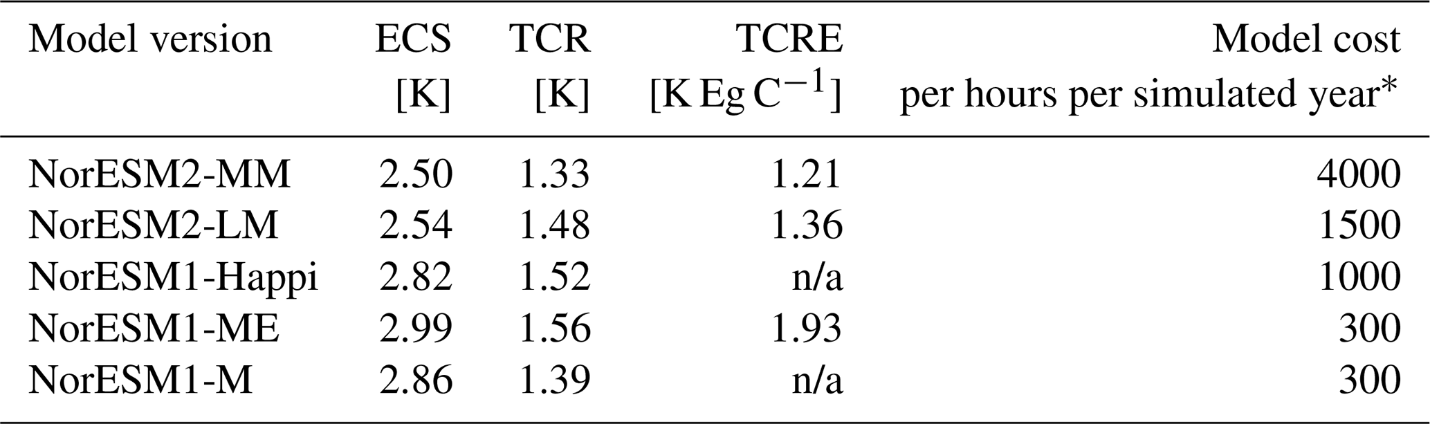
aIntel compiler with -O2 and -xAVX options, 1024 pes, single-threaded MPI on Lenovo NeXtScale M5 cluster, 32-way nodes, dual 16-core Xeon E5-2683 at 2.10 GHz, 64 GiB per node. Timing is system and compiler dependent, and approximate only. n/a – not applicable
In NorESM2, one specific modification was made to the surface water treatment in CLM. The surface water pool is a new feature replacing the wetland land unit in earlier versions of CLM (introduced in CLM4.5). This water pool does not have a frozen state but is added to the snowpack when frozen. To avoid water being looped between surface water and snow during alternating cold and warm periods, we remove infiltration excess water as runoff if the temperature of the surface water pool is below freezing. This was done to mitigate a positive snow bias and an artificial snow depth increase found in some Arctic locations during melting conditions.
2.7 Coupler
The state and flux exchange between model components and software infrastructure for configuring, building, and execution of model experiments is handled by the CESM2 coupler Common Infrastructure for Modeling the Earth (CIME; Danabasoglu et al., 2020). The coupler computes the turbulent air–sea fluxes of heat and momentum, and in NorESM2 this is implemented as a version of the Coupled Ocean-Atmosphere Response Experiment version 3 (COARE-3) (Fairall et al., 2003) scheme, replacing the calculation based on Large and Yeager (2004) in CESM2. State and flux exchange via the coupler between atmosphere, land, and sea-ice components occurs half-hourly, aligned with the atmosphere time step, while the ocean exchanges with the coupler every hour. CIME also provides common utility functions and among these are estimation of solar zenith angle. In NorESM2, this utility function is modified with associated changes in atmosphere, land, and sea-ice components, ensuring that all albedo calculations use a zenith angle averaged over the component's time step instead of instantaneous angles.
Most of the general development of the model as described in Sect. 2 was tested in configurations with a reduced number of interactive components. CAM6-Nor was tuned in Atmospheric Model Intercomparison Project (AMIP) configuration with mean climatological radiative forcings and boundary conditions (sea-surface temperatures – hereafter SSTs – and sea ice) derived from observations over the period 1990–2010. Similarly, BLOM and iHAMOCC were primarily tuned with prescribed atmosphere and runoff forcing of the OMIP1 protocol. The scope of these separate experiments was to test improved representations of the physical processes in the simulations, with the twin aims of mitigating model systematic biases when compared to the observed climate and achieving a net radiative flux imbalance at the top of the model atmosphere (hereafter RESTOM; defined as positive inward, i.e. warming the climate) more in line with satellite-based estimates, given the observed SSTs.
The first coupled version of NorESM2 included all changes described in Sect. 2. This version was heavily tested in a pre-industrial setting (as defined in Sect. 4).
This initial version of the coupled model was initialised using a hybrid of observational estimates and earlier model simulations. The ocean model was initialised with zero velocities and temperature and salinity fields from the Polar science center Hydrographic Climatology (PHC) 3.0 (updated from Steele et al., 2001). Following the OMIP protocol (Orr et al., 2017), the nutrients (phosphate, nitrate, and silicate) and oxygen fields in NorESM2 were initialised with the gridded climatological fields of the World Ocean Atlas database (Garcia et al., 2014a, b). For dissolved inorganic carbon and total alkalinity, we used the pre-industrial and climatological values from the Global Ocean Data Analysis Project (GLODAPv2) database (Lauvset et al., 2016). Other biogeochemical tracers are initialised using values close to zero. CAM and CLM were initialised using the files included in the CESM2 release. Aerosols and aerosol precursors were initialised to near-zero values. As there were no low-resolution pre-industrial initial files for the land model available, this was replaced by an interpolation of the 1∘ initial file from CESM2. At a later stage in the coupled spin-up, the land surface fields were re-initialised from a long (approximately 1400 years) stand-alone CLM spin-up simulation driven by repeating 50 years of coupling exchange fields obtained from the earlier coupled run.
Similar to CESM, NorESM2 adjusted towards its own coupled climatology with an initial phase of strong cooling in the high latitudes of the Northern Hemisphere, after which an intensification of ocean heat advection stabilised the simulation. After that point, the climatology tended to settle towards a steady state. During major tuning steps, the coupled model had to be restarted from the initial state several times. In order to save computer resources, minor tuning, especially towards reducing RESTOM, was performed on the best-candidate simulation after this initial, large adjustment. Alongside the final tuning, the CESM components were updated to the versions found in CESM2.1. The changes from CESM2.0 to CESM2.1 are mostly technical but also include minor bug fixes and updated forcing fields (Danabasoglu et al., 2020). The update was done after an initial adjustment but early in both spin-ups, approximately 1000 model years before the start of the control, at both resolutions. The impact on the global fields is quite small, as can be seen in Figs. S1 and S2 in the Supplement. In this second phase of coupled spin-up, it was found that the sensitivity of some aspects of the simulated coupled climatology to small changes in parameters or parameterisations could be different than that found in stand-alone simulations of the individual components with prescribed boundary conditions. The coupled response could be both amplified or damped with respect to single-component simulations. As a result, some of the final parameter tuning of the model had to be performed in coupled mode. No tuning was performed during the pre-industrial control simulation as described in Sect. 4.1
The main goal of the coupled tuning process was to create an energy-balanced pre-industrial control simulation with a reasonably stable, adjusted equilibrium state. The simulation can produce a steady climatology only if the time-average radiative imbalance on the top of the model vanishes. In practice, a commonly used target is to bring RESTOM to within ±0.1 W m−2 while maintaining values of mean atmospheric and ocean temperatures close to observations. To achieve this, each change in the coupled model was tested in parallel in atmosphere-only (AMIP) and ocean-only (OMIP) modes. As ocean heat gain and tropospheric air temperature, humidity, and cloudiness are strongly associated with the fluxes at the top of the atmosphere, improving the state in the coupled simulation and reducing RESTOM and drift in AMIP and OMIP simulations are closely connected goals. On the other hand, fine tuning of the coupled state should not significantly degrade important climatological variables such as temperature, precipitation, clouds, or the main mode of coupled variability, i.e. ENSO. Our parallel testing procedure ensured that the model simulation maintained a degree of consistency both with the present-day observed climatology and with a steady pre-industrial climate. Where available, notably in SST and sea ice, observational estimates of the state of Earth's pre-industrial climate were also considered against the coupled integrations. Each tuning step was performed in isolation, and an effort was made to ensure the greatest possible similarities in the two model configurations (LM and MM). No tuning was performed that attempted to target other modes of variability besides ENSO, or a particular climate response to external forcings, e.g. from changes in greenhouse gas concentration, anthropogenic aerosol emissions, or volcanic or solar forcing.
Similar to CESM2 (Danabasoglu et al., 2020), NorESM2 tended to develop excessive sea-ice cover in the Labrador Sea (LS) region, although the temporal development in NorESM2 differed from CESM2. For any tested combination of parameter choices, NorESM2 developed excessive LS sea-ice cover starting around year 60 after model initialisation. This was however only a temporary model state and in all experiments the sea ice returned close to observed state in the LS region after additional 60–80 model years of simulation.
One of the most common methods to tune RESTOM is to change the amount and thickness of low clouds. The main parameter used for tuning the low clouds in the Cloud Layers Unified By Binormals (CLUBB) scheme is the “gamma” parameter, which controls the skewness of the assumed Gaussian probability density function for subgrid vertical velocities. A low gamma implies weaker entrainment at the top of the clouds, in particular for marine stratocumulus. This increases the amount of low clouds and results in a higher short-wave cloud forcing.
Given the same gamma values, the RESTOM was higher in the low-resolution version of the model. In addition, the sensitivity to the change of the gamma parameter was different in the two model resolutions, so a different choice of gamma was needed for the two resolutions. The final parameter values are well within the gamma range of 0.1–0.5 tested by Zhang et al. (2018), although smaller than the values used in CESM2 at the same resolution. A small gamma pushes up short-wave cloud radiative forcing (SWCF), which led to a high bias in SWCF in NorESM2-LM. This bias was somewhat offset by regulating the parameter dcs (autoconversion size threshold for cloud ice to snow), with a small impact on the tropospheric temperature bias.
While the amount of change in SWCF could be estimated by running the atmosphere and land model in a stand-alone configuration, the change in RESTOM in coupled setup was small compared to the change in cloud forcing. Further attempts at reducing positive RESTOM by tuning the boundary-layer stability were neutralised by SST adjustment while worsening the tropospheric cold bias. A more effective tuning of low cloud radiative effects was achieved by modifying air–sea fluxes of DMS. Compared to Schwinger et al. (2017), the parameter controlling DMS production by diatoms was doubled in NorESM2, which allowed us to maintain high DMS concentration at high latitudes during spring and summer seasons in both hemispheres, as in observations (Lana et al., 2011). This tuning compensates for the reduced primary production simulated in NorESM2 compared to that in NorESM1 (Tjiputra et al., 2020).
RESTOM was decisively reduced, both in stand-alone (AMIP) and in coupled simulations (before SST adjustment), by increasing outgoing long-wave radiation. This was achieved in three ways. First, alterations were made to the Zhang and McFarlane (1995) convection scheme, as described in Toniazzo (2020), aimed at increasing mid- and high-altitude latent heating of the atmosphere for a given amount of precipitation. Second, positive cloud radiative forcing in the terrestrial radiation spectrum was reduced by intervening on the parameterisation of ice-cloud fraction. Finally, higher sea-surface temperatures in coupled simulations were achieved by reducing the value of the parameter controlling background vertical mixing in the ocean back to that used in NorESM1. Initial optimisation in stand-alone configurations had led to increase the value of this parameter by about 50 %.
A remarkable sensitivity of the model climatology to the parameterisation of the ice-cloud fraction was found. This purely empirical part of the cloud parameterisation of CESM2 is rather ad hoc and poorly constrained by observations. Several namelist-controlled options for ice-cloud fraction are provided in CESM. Initial tuning of the parameters of the CESM2 default option appeared promising, but coupled adjustment again tended to neutralise the effect on model radiative imbalance. In NorESM2-LM, an effective reduction in the high- and mid-level cloud cover could only be achieved by switching to a different parameterisation option, in which there is no direct functional dependence of ice-cloud fraction on environmental relative humidity (this is option number 4 in CESM). By contrast, in NorESM2-MM, the CESM default scheme (option number 5, with explicit RH dependence) could be modified by allowing a continuous narrowing of the range of cloud sensitivity to environmental RH. This modification thus constitutes a continuous switch between the two parameterisation options. A target for future development might be to represent ice clouds in a way better rooted in physical processes.
We give a concise summary of the parameters that were used for tuning NorESM2, with their final value and a comparison with CESM2, in Table 2.
Table 2 Tuning parameters of NorESM2-LM and NorESM2-MM. Compared to CESM2 (Danabasoglu et al., 2020) where applicable.
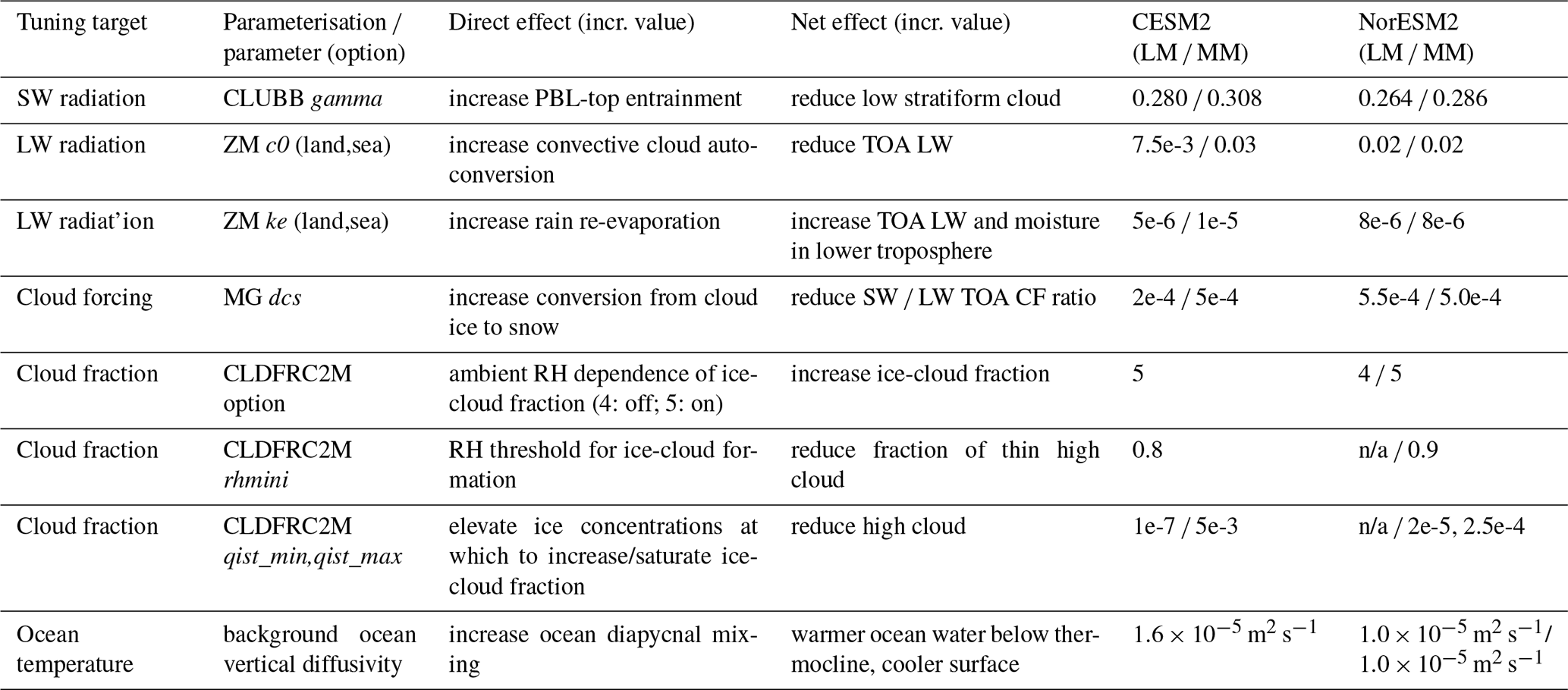
n/a – not applicable
This section presents a basic description of the climatology simulated in CMIP6 experiments with the two versions of the model, NorESM2-LM and NorESM2-MM (Sect. 2.1). We consider the time evolution of temperature in historical and enhanced greenhouse gas future climate scenarios, along with aspects of the ocean circulation and sea ice. We validate the historical coupled simulations against observational estimates and reanalyses, and compare them with results from simulations with previous versions of NorESM (Sect. 5): NorESM1-M (Bentsen et al., 2013; Iversen et al., 2013; Kirkevåg et al., 2013) used in CMIP5 and NorESM1-Happi (Graff et al., 2019) used for HAPPI (Half a degree Additional warming Prognosis and Projected Impacts; Mitchell et al., 2017) and a set of CMIP5 experiments carried out for model evaluation purposes (Graff et al., 2019). NorESM1-Happi is an upgraded version of NorESM1-M with differences including doubled horizontal resolution in the atmosphere and land components (1∘ in NorESM1-Happi and 2∘ in NorESM1-M) and improved treatment of sea ice. The motivation for including NorESM1-Happi in the present paper is to present results from a low-resolution (-M) and medium-resolution version (-Happi) of NorESM1 alongside the results from the low-resolution (-LM) and medium-resolution (-MM) versions of NorESM2.
We consider three sets of experiments that are important for documentation and application of CMIP6 models: the DECK (Diagnostic, Evaluation, and Characterization of Klima) experiments (Eyring et al., 2016), the CMIP6 historical experiment (Eyring et al., 2016), and the tier 1 experiments of the Scenario Model Intercomparison Project (ScenarioMIP) (O'Neill et al., 2016). A brief description of the setup of these experiments is given in Sect. 4.1.
The analysis is divided into three parts. Section 4.2 focuses on the stability of the pre-industrial control simulation. In Sect. 4.3, we consider the simulated climate sensitivity to abrupt and gradual quadrupling of CO2. A brief analysis of the warming, sea ice, the Atlantic Meridional Overturning Circulation (AMOC), and the transport through the Drake Passage in the historical simulations and the scenarios is given in Sect. 4.4.
4.1 Experiment setup
As described by Eyring et al. (2016), a set of common experiments known as DECK has been defined to better coordinate different model intercomparisons and provide continuity for model development and model progress studies. DECK consists of the following four baseline experiments: (1) the historical AMIP experiment; (2) the pre-industrial control (piControl) experiment defined by estimated forcings from 1850, started from initial conditions obtained from a spin-up with the same, constant forcings during which the coupled model climatology stabilises towards stationary statistics; (3) an experiment otherwise identical to piControl, except that the CO2 concentrations are set to 4 times the piControl concentrations, from piControl initial conditions (abrupt-4xCO2); (4) an experiment otherwise identical to piControl but where the CO2 concentrations are gradually increased by 1 % per year starting from piControl concentrations and initial conditions (1pctCO2). Both abrupt-4xCO2 and 1pctCO2 were started from year 1 of the control. DECK was produced with both versions of the model (NorESM2-LM and NorESM2-MM), and here we consider results from the pre-industrial control and the abrupt-4xCO2 and 1pctCO2 (Sect. 4.2–4.3). As this paper focuses on the coupled aspect of NorESM2, the AMIP runs are not included here but are described in Olivié (2020) and Toniazzo (2020).
Another qualifying experiment required for entry in CMIP6, and important for model evaluation with respect to observations, is the historical experiment. In this experiment, time-dependent forcings are specified to reflect observational estimates valid for the so-called historical period, viz. 1850–2014. Following CMIP6 guidelines, for this experiment, we carried out a small ensemble of integrations, consisting of three members. This helps isolate the forced signal from internal climate variability. The three model integrations of the ensemble differ only in their initial conditions, which were obtained from model states late in the spin-up at intervals of 30 model years apart. This is analogous to the historical ensemble of NorESM1 produced for CMIP5.
Beyond DECK, one of the most important applications for ESMs is to provide estimates of future climate change. This is typically done using scenarios which specify future anthropogenic forcing of the climate that include changes in land use (such as deforestation) and the addition of greenhouse gases and other pollutants to the atmosphere. The latter can be prescribed either directly as atmospheric concentrations (as a function of time) or as time evolving in emissions into the atmosphere (which then interact with ocean and land biogeochemical processes before yielding atmospheric concentrations). The design of scenarios is based on a combination of socioeconomic and technological development, named the Shared Socioeconomic Pathways (SSPs), with future climate radiative forcing (RF) pathways, Representative Concentration Pathways (RCPs), in a scenario matrix architecture (Gidden et al., 2019).
The simulations included in this paper are the tier 1 experiments of ScenarioMIP (O'Neill et al., 2016): SSP1-2.6, SSP2-4.5, SSP3-7.0, and SSP5-8.5. The forcing fields for all the experiments are generally the same as those used in CESM2.1. This includes solar forcing, prescribed oxidants used for describing secondary aerosol formation, greenhouse gas concentrations, stratospheric H2O production from CH4 oxidation, ozone used in the radiative transfer calculations, and land use. While the experiments in this paper use prescribed greenhouse gas concentrations, NorESM2 can also be run with CO2 emissions as described by Tjiputra et al. (2020).
NorESM2 lacks a physical representation of the stratosphere; instead, appropriate upper-boundary conditions need to be specified. Accordingly, stratospheric aerosols and emissions of aerosols and aerosol precursors were prescribed based on the data provided by the input4mips website: https://esgf-node.llnl.gov/projects/input4mips/ (last access: 1 December 2020). In addition, sulfur from tropospheric volcanoes was included similarly to Kirkevåg et al. (2018); see Sect. 2.2.
4.2 Simulated control climatology and residual drift
After tuning and an initial spin-up, both NorESM2-LM and NorESM2-MM were integrated for 500 years with steady pre-industrial forcings to produce the piControl experiments. Below, we present a basic analysis of the general state and drift of important parameters of the simulated climatology.
During the control integration, the forcings as well as the parameter choices were kept constant. There should be no long-term drift in the model state variables or their partial tendencies (hence, a fortiori, in radiative fluxes). More precisely, any residual drift of the simulated control climatology should be negligibly small compared with the signal resulting from the response to changes in climate forcings as prescribed in the historical, enhanced greenhouse gas, and scenario experiments. In practice, a reasonable target is to maintain the RESTOM of piControl within ±0.1 W m−2 in the time mean. Any small imbalance in RESTOM is typically reflected in a small trend in ocean temperature. A time series of AMOC can give an indication of the stability of the general ocean circulation.
Figure 2 shows time series of related global means in the piControl simulations from NorESM2-LM and NorESM2-MM. As can be seen in the figure, the drift is generally small and comparable for the two model versions. The top-of-the-atmosphere radiative imbalance is −0.057 W m−2 for NorESM2-LM and −0.065 W m−2 for NorESM2-MM. The ocean volume temperature change of 0.03 K over 500 years is much smaller than the rate of warming observed during the last 50 years. Similarly, there are positive trends in global-mean ocean salinity of and g kg−1 over 500 years for NorESM2-LM and NorESM2-MM, respectively, that we consider small since for NorESM2-MM this is equivalent to an average surface freshwater loss of mm d−1. The remaining trends are not significantly different from 0 % at the 95 % confidence level, as estimated from a t test. We found however a slight decrease in DMS sea-to-air flux of 2 % over the 500-year control period, reflecting a residual drift in ocean biogeochemistry. AMOC variations are reasonably small and show no significant trend.
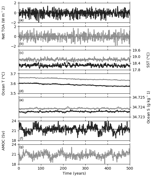
Figure 2Pre-industrial control experiment characteristics for NorESM2-LM (black lines) and NorESM2-MM (grey lines). Time evolution of globally averaged top-of-the-atmosphere (TOA) net radiative balance (first and second panel from top), sea-surface temperature (SST) (third panel), ocean temperature (fourth panel), ocean salinity (fifth panel), and AMOC at 26.5∘ N (bottom two panels) for model years 0–500.
4.3 Equilibrium climate sensitivity and transient response
The two enhanced greenhouse gas experiments of the CMIP-DECK were started at the same initial conditions as piControl (and consequently assigned the same notional model year). They are referred to as abrupt-4xCO2 and 1pctCO2.
Figure 3 shows the time evolution of near-surface temperature for abrupt-4xCO2, 1pctCO2, and piControl for both model configurations. Three commonly used metrics for the response to CO2 forcing, based on the evolution of the simulated global-mean temperature, are the equilibrium climate sensitivity (ECS), the transient climate response (TCR), and the transient climate response to cumulative CO2 emissions (TCRE). Their values are given in Table 1 for the NorESM2 experiments and compared to those for NorESM1. The ECS is defined as the change in global near-surface temperature when a new climate equilibrium is obtained with an atmospheric CO2 concentration that is doubled compared to the pre-industrial amount. In order to reach a new equilibrium, a model simulation of several thousand years is required (Boer and Yu, 2003). There are some examples in the literature of models for which this has been done; e.g. Paynter et al. (2018) show results from simulations with GFDL-CM3 and GFDL-ESM2 run for more than 4000 years. Given certain assumptions, ECS may be estimated from the relationship between surface temperature and RESTOM from the abrupt-4xCO2 experiment using the so-called Gregory method (Gregory et al., 2004). This estimate has become a standard in CMIP6. The figures reported in Table 1 are calculated using years 1–150 from the simulations shown in Fig. 3 and are divided by 2 to get the number for CO2 doubling instead of quadrupling. The ECS is 2.54 K for NorESM2-LM, which is slightly lower than the equivalent value for NorESM1 of 2.8 K. Both are significantly lower than the CMIP5 mean value of 3.2 K but well inside the bounds of the likely range of 1.5–4.5 K (Stocker et al., 2013). On the other hand, the ECS in NorESM2 is markedly smaller than the ECS found in CESM2 of 5.3 K by Gettelman et al. (2019a), despite sharing many of the same component models. An extensive analysis of the low ECS value in NorESM2 is given in Gjermundsen et al. (2020). Note that the aerosol forcing is not very different between NorESM2 and CESM2 and cannot explain the discrepancy in ECS values. Several sensitivity experiments have been conducted and are reported in Gjermundsen et al. (2020) in order to investigate the importance of different ice-cloud schemes, CLUBB, and interactive DMS. However, these NorESM2 experiments exhibit similar ECS values. The main reason for the low ECS in NorESM2 compared to CESM2 is how the ocean models respond to GHG forcing. The behaviour of the BLOM ocean model (compared to the POP ocean model used in CESM2), contributes to a slower surface warming in NorESM2 compared to CESM2. Using the Gregory et al. (2004) method on the first 150 years leads to an ECS estimate which is considerably lower than for CESM2. However, if 500 years are included in the analysis, NorESM2 shows a sustained warming similar to CESM2. This suggests that the actual equilibrium temperature response to a large GHG forcing (the value one finds when the model is run for many hundreds of years) in NorESM2 and CESM2 is not very different, but that the Gregory et al. (2004) method based on the first 150 years does not give a good estimate of ECS for models.
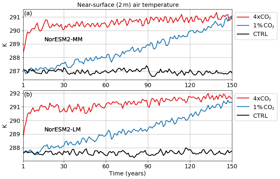
Figure 3Time evolution of globally averaged near-surface temperature in NorESM2-MM (a) and NorESM2-LM (b) for the pre-industrial control simulation, the abrupt-4xCO2 experiment, and the gradual increase 1pctCO2 experiment for model years 1–150.
The TCR is defined as the global-mean surface temperature change at the time of CO2 doubling, and accordingly it was calculated from the temperature difference between the 1pctCO2 experiment averaged over years 60–80 after initialisation and piControl. The TCR is 1.48 K and 1.33 K for NorESM2-LM and NorESM2-MM, respectively. As for ECS, these values fall in the lower part of the distribution obtained from the CMIP5 ensemble (Forster et al., 2013), similar to those obtained for NorESM1. The TCR of both NorESM2-LM and NorESM2-MM are lower than the value of 2.0 K found for CESM2 (Danabasoglu et al., 2020). A recent observational estimate for the 90 % likelihood range of TCR is 1.2–2.4 K (Schurer et al., 2018).
We also give an estimate of the transient climate response to cumulative carbon emissions (TCRE) calculated from TCR and the corresponding diagnosed carbon emissions. Following Gillett et al. (2013), TCRE is defined as the ratio of TCR to accumulated CO2 emissions in units of K Eg C−1. As CO2 fluxes were not calculated in NorESM1-M and NorESM1-Happi, the NorESM1 values are obtained from the carbon-cycle version of NorESM1 (NorESM1-ME; Tjiputra et al., 2013). TCRE is reduced from 1.93 K Eg C−1 in NorESM1-ME to 1.36 and 1.21 K Eg C−1 in NorESM2-LM and MM, respectively. Since TCR is comparable, the main difference is due to changes in carbon uptake. NorESM1, with CLM4 as the land component, had a very strong nitrogen limitation on land carbon uptake. This limitation is weaker in CLM5 (Arora et al., 2019) used in NorESM2.
4.4 Climate evolution in historical and scenario experiments
In this section, we provide a very brief analysis of the response of the model to historical forcings in the three historical members carried out in both NorESM2-LM and NorESM2-MM. We also consider the model response for the tier 1 experiments from ScenarioMIP (SSP1-2.6, SSP2-4.5, SSP3-7.0, and SSP5-8.5). The focus here will be on the response in global-mean near-surface temperature, the AMOC, the volume transport through the Drake Passage, and sea-ice area.
Figure 4 shows the time evolution of the surface atmospheric temperature in the historical simulations from NorESM2-LM and NorESM2-MM along with observations. Both versions of NorESM2 follow the observations rather closely for the first 80 years. After 1930, the model displays somewhat weaker warming than the observations until around 1970. After that, the rate of the warming in the models is similar to that seen in the observations. The cooling over the period 1930–1970 in NorESM2 is probably caused by the combination of a low climate sensitivity (see Sect. 4.3) and a strong negative aerosol forcing. Atmosphere-only simulations with NorESM2-LM (see Olivié, 2020) show that the aerosol effective radiative forcing (ERF) strengthens from around −0.3 W m−2 around 1930 to −1.5 W m−2 in the period 1970–1980, becoming slightly weaker again in 2014 with a value of −1.36 W m−2. On a global scale, anthropogenic SO2 emissions have risen strongly in the period 1950–1980, and these are assumed to contribute most to the anthropogenic aerosol forcing. The ERF is quite similar in both model versions. We find an ERF of W m−2 in NorESM2-LM and W m−2 in NorESM2-MM for the year 2014 (compared to 1850). Figure S3b shows the time evolution of ERF for the first ensemble member of NorESM2-LM. Given that the ERF is not an observable quantity, we have also included time series of aerosol optical depth which can be related to measurements (Fig. S3a) along with a comparison of aerosol optical depth with observations (Fig. S4). Detailed analysis of the aerosol properties is done in Olivié (2020). Note also that our choice of the reference period for temperature anomaly computation (1850–1880) enhances the NorESM2 negative bias with respect to observations in the last half of the 20th century.
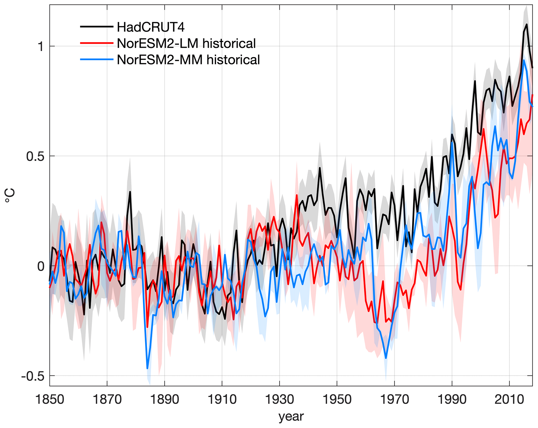
Figure 4Time evolution of globally averaged surface temperature in the historical simulations of NorESM2-LM (red line) and NorESM2-MM (blue line) shown with the observations (black line) from the Hadley Centre – Climate Research Unit Temperature dataset version 4 (HadCRUT4) (Morice et al., 2012) updated to version HadCRUT4.6.0.0. Temperatures are computed as anomalies from the time mean over the years 1850–1880. For NorESM2-LM and NorESM2-MM, the solid lines show the mean and the shading of corresponding colour the spread from three ensemble members. For HadCRUT4, the solid black line shows the median and the grey shading indicates the lower and upper bounds of the 95 % confidence interval of the combined effects of all the uncertainties described in the HadCRUT4 error model (measurement and sampling, bias, and coverage uncertainties).
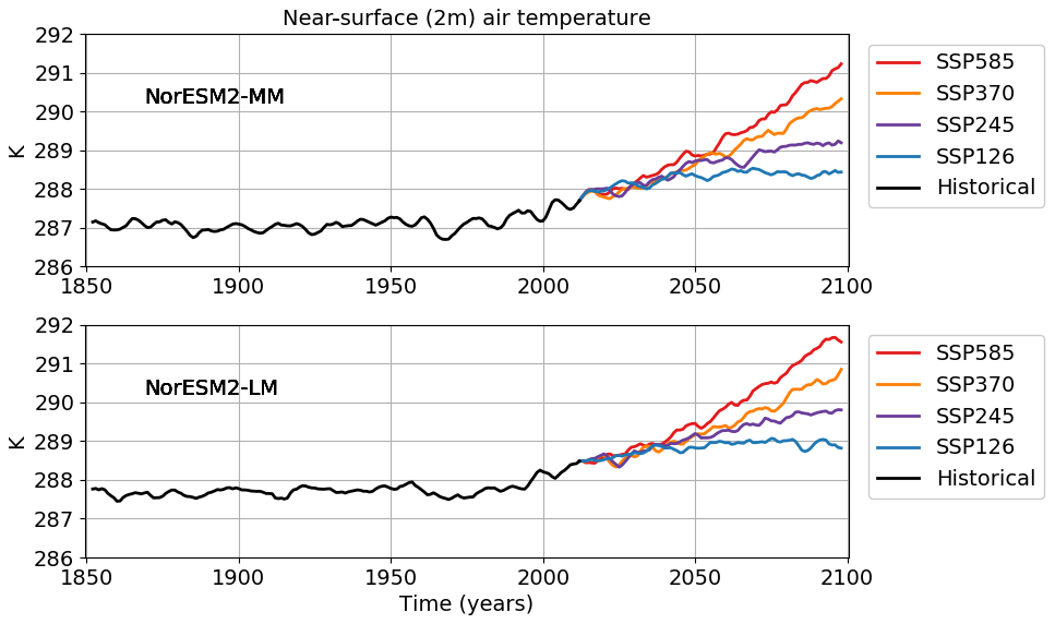
Figure 5Time evolution of globally averaged surface air temperature in NorESM2-MM and NorESM2-LM from the historical simulations (black lines) and CMIP6 scenario experiments SSP1-2.6, SSP2-4.5, SSP3-7.0, and SSP5-8.5 (coloured lines). A 5-year moving average is used.
Figure 5 shows again the evolution of the surface air temperature in the historical simulations (only the first ensemble member for NorESM2-LM), followed by the temperature evolution under the four SSP scenarios for NorESM2-LM and NorESM2-MM. Compared to the 1850–1879 period, the model shows a warming in 2005–2014 of 0.72 and 0.54 K for NorESM2-LM and NorESM2-MM, respectively. Under the four scenarios (SSP1-2.6, SSP2-4.5, SSP3-7.0, and SSP5-8.5), the warming in the period 2090–2099 compared to 1850–1879 reaches 1.30, 2.15, 2.95, and 3.94 K in NorESM2-LM, and 1.33, 2.08, 3.06, and 3.89 K in NorESM-MM. The absolute temperature simulated by LM is almost 1∘ warmer than MM throughout the 1850–2100 period, but anomalies are similar. For SSP1-2.6, the temperature stabilises in the second half of the 21st century. In NorESM1, under the RCP2.6, RCP4.5, and RCP8.5 scenarios, the surface air temperature in the period 2071–2100 was 0.94, 1.65, and 3.07 K higher than in 1976–2005 (Iversen et al., 2013). For the same periods and looking at SSP1-2.6, SSP2-4.5, and SSP5-8.5, we find rather similar (but slightly stronger) warmings of 1.06, 1.81, and 3.22 K in NorESM2-LM, and 1.11, 1.83, and 3.26 K in NorESM2-MM.
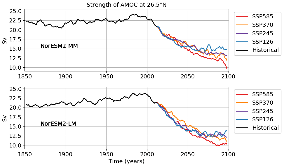
The simulated AMOC at 26.5∘ N shows a multi-centennial variability that is 15 % of the mean in the control simulation (Fig. 2). In the historical simulations, the AMOC peaks for both MM and LM in the 1990s at around 24 Sv before starting a rapid decline at around the year 2000 (Fig. 6). In both versions, the AMOC reaches a quasi-equilibrium by the end of the century at around 15–10 Sv depending on the scenario. Since we only have a few ensemble members, it remains unclear how fast the AMOC declines in response to the greenhouse gas forcing and which part of, e.g. the initial decline is due to the multi-decadal variability. In any case, it is noteworthy that the initial AMOC decline begins already during the historical period in both versions, which is also consistent with the NorESM2 and multi-model mean response to the OMIP2 forcing (1958–2018, Tsujino et al., 2020).
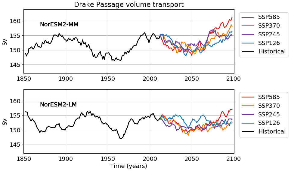
In addition to the AMOC, also the Antarctic Circumpolar Current (ACC) strength, as measured in the Drake Passage, shows multi-centennial variability that is about 3 % of the mean (Fig. 7). Similar variability in the ACC has been linked to convection within the Weddell and Ross seas in the CMIP5 ensemble (Behrens et al., 2016). Also, in our simulations, the Weddell Sea convection has similar long-term variability to the ACC. Unlike the AMOC, there is no clear trend emerging from the scenario simulations, but rather the multi-decadal variability continues throughout the 21st century. Again, a larger number of ensemble members could help identify the forced signal.
The time evolution of Northern Hemisphere sea-ice area (March and September) through the historical and scenario periods is shown in Fig. 8. Both model versions are compared with the sea-ice area from the Ocean and Sea Ice Satellite Application Facility (OSISAF) (OSI-V2.0) reprocessed climate data record (Lavergne et al., 2019) for the years 1979–2019. The total sea-ice area from NorESM2-LM compares rather well with the observations, while NorESM2-MM has too much ice, especially during summer. The trend in sea-ice area found in the observations during summer is also rather well captured by NorESM2-LM, while this trend is too small in NorESM2-MM. Both models have a reasonable March sea-ice area compared to observations. However, the negative trends in winter sea-ice area are small compared to observed trends.
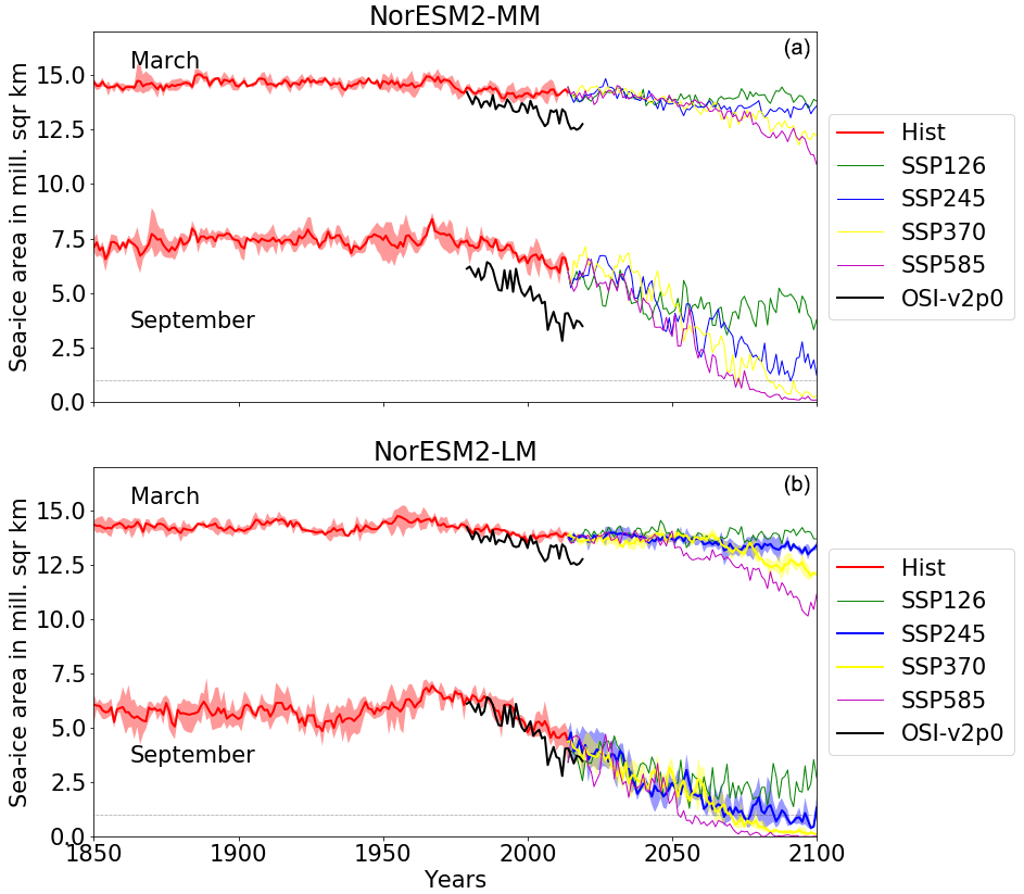
Figure 8Northern Hemisphere sea-ice area for March and September for historical and scenario experiments: (a) NorESM2-MM and (b) NorESM2-LM. Black lines show observations from OSISAF (Lavergne et al., 2019) for the years 1979–2019. Ensemble means, with shades for ensemble range, are shown for both model configurations for the historical (1850–2014) and for the SSP2-4.5 (2015–2100) and SSP3-7.0 (2015–2100) scenarios from NorESM2-LM. The rest of the lines denotes only one realisation.
During the scenario period, both models show a strong reduction in summer sea-ice area. The Arctic Ocean is often considered ice-free when the total sea-ice area drops below 1 million km2. This threshold is denoted by dotted grey lines in Fig. 8. NorESM2-LM loses summer ice shortly after the year 2050. This occurs first in the SSP5-8.5 scenario, but also the SSP2-4.5 ensemble shows values close to this threshold even before 2050. SSP3-7.0 scenarios become ice-free at around 2070. Any prediction of which year the Arctic Ocean first becomes ice-free must therefore be considered rather uncertain due to forcing evolution uncertainty and internal variability. This is consistent with the overall assessment of sea-ice evolution in CMIP6 assessed by the SIMIP Community (2020). In NorESM2-LM, an ice-free Arctic Ocean is only avoided in the SSP1-2.6 scenario. NorESM2-MM loses ice slower and shows the first ice-free summer around 2070. In that model, also the SSP2-4.5 scenario keeps the ice area above 1 million km2 all years before 2100. However, the SSP1-2.6 scenario stabilises at a sea-ice area comparable with present-day observations, even with SSP1-2.6 warming levels present. Therefore, the sea-ice area simulated by NorESM2-MM for the future Arctic seems to be unrealistically high.
5.1 Ocean state
In the surface ocean, the large-scale climatological biases are similar in the two NorESM2 versions (Fig. 9), but overall the MM version is closer to the observations (smaller global-mean root-mean-square error, RMSE; in Fig. 9). In general, the Southern Ocean is too warm (Fig. 9b–c), the Atlantic and the Arctic are too saline, but the Pacific is too fresh (Fig. 9e–f). The sea-level anomaly is lower than observed in the Atlantic basin but higher in the Indo-Pacific basin, and thus the gradient between the two basins is larger than in the observations (Fig. 9h–i). If we remove the global-mean biases, the two versions produce even more similar mean errors, suggesting that some of the regional biases are largely independent of the atmosphere and land resolution.
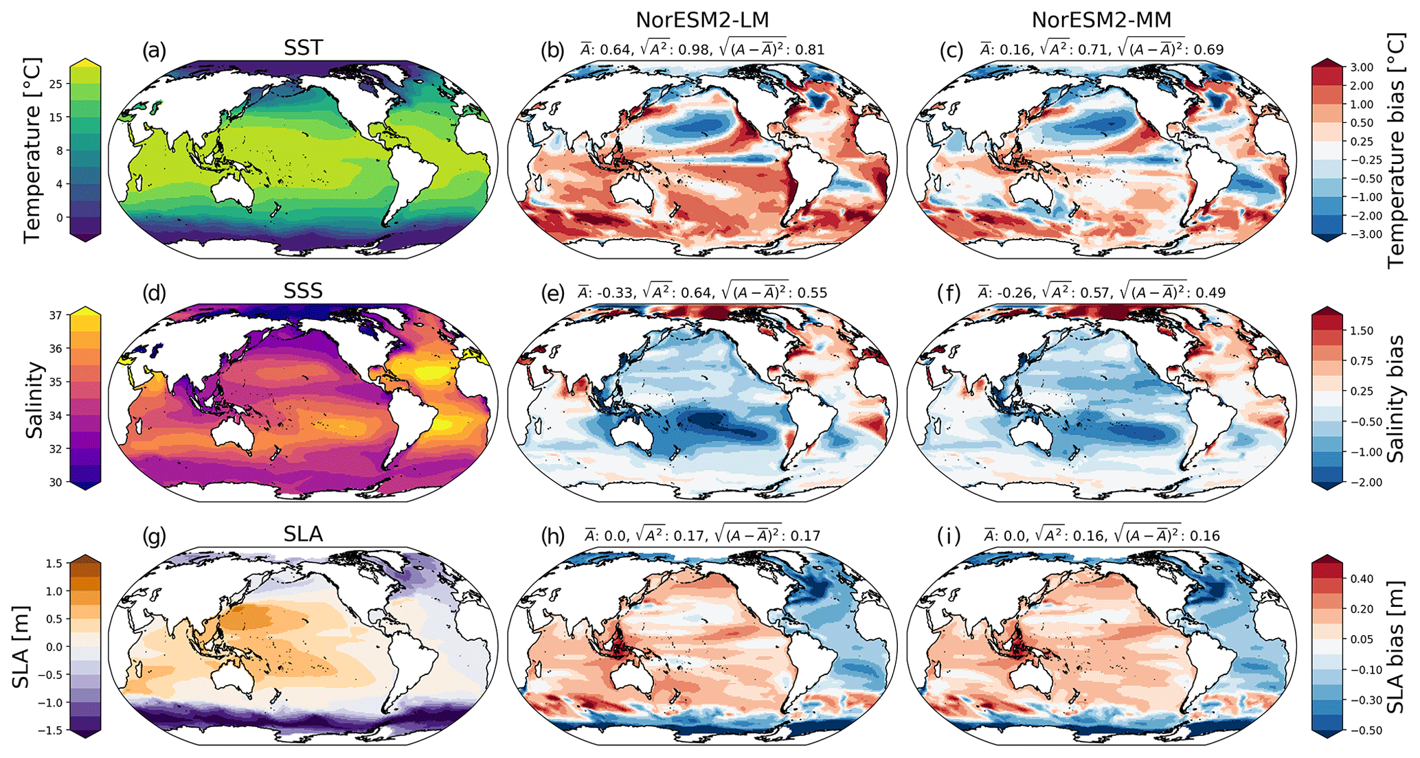
Figure 9Observed climatologies (a, d, g) and biases for NorESM2-LM (b, e, h) and NorESM2-MM (c, f, i) for SST, sea-surface salinity (SSS), and SLAs. SST and SSS are compared to the World Ocean Atlas climatology (Locarnini et al., 2018; Zweng et al., 2018) between 1981 and 2010, whereas SLA is compared to Aviso altimetry between 1993 and 2010. For the model biases, we show the ensemble-mean bias using three historical members. Note that A is the anomaly between the model and the observation, and we report the global-mean bias (), global-mean RMSE (root-mean-square error; ), and global-mean RMSE with the mean bias first removed (). SLA is redefined to have zero mean over the ice-free region in the observational dataset (thus, is 0 by definition).
Indeed, the regional patterns are common to many other models with coarse-resolution ocean components (Wang et al., 2016). Both NorESM2 versions are too warm and (relatively) saline over the western boundary currents (the Gulf Stream and the Kuroshio in the Northern Hemisphere and the Brazil Current and the Agulhas Current in the Southern Hemisphere) and over the major eastern boundary upwelling systems (Canary, Benguela, Humboldt, and California). The biases over the western boundary currents are due to the errors in the location of the currents, which are linked to the ocean-model resolution (Bryan et al., 2007; Saba et al., 2016; Rackow et al., 2019). The ocean-model resolution also explains two well-known biases in the North Atlantic also seen in NorESM2: the southern bias in the Gulf Stream–North Atlantic current path causes the cold (and fresh) bias in the subpolar North Atlantic (Bryan et al., 2007; Saba et al., 2016; Rackow et al., 2019), while the lack of the Labrador Current waters on the east coast of North America causes a large warm and saline bias there (Saba et al., 2016).
While the abovementioned biases are mostly linked to the ocean model, in the Pacific there are biases that are not present in the ocean-only simulations (not shown). Specifically, a fresh bias over the southern Pacific subtropical gyre and cold biases over the northern Pacific subtropical gyre and the equatorial Pacific.
The fresh bias in the southern Pacific (Fig. 9) is linked to the co-located positive net precipitation bias as shown in Fig. 19 and extends throughout the surface mixed layer (Fig. 11). The salinity bias also causes a negative density bias (not shown) as it is not fully compensated by temperature, supporting an atmospheric origin. A comparison with the OMIP1 and OMIP2 simulations shows that the net precipitation bias in the LM simulation, 250 mm yr−1 in the mean over the region where the salinity bias is larger than 1 g kg−1, would be large enough to cause the simulated salinity bias (assuming mixed layer depth of 100 m and a residence time of 10 years). Therefore, we suggest that the net precipitation bias leads to accumulation of excess freshwater that is spread throughout the subtropical gyre by the ocean circulation.

Figure 10Zonal-mean bias in potential temperature for NorESM2-LM and NorESM2-MM. The bias is taken relative to World Ocean Atlas climatology (Locarnini et al., 2018; Zweng et al., 2018) using the years 1981–2010 in the main ocean basins. Note the change in the vertical scale between the upper 500 m and the lower 4500 m. For the model biases, we show the ensemble-mean bias using three historical members.
Most of the large-scale surface biases are also visible in the subsurface (Figs. 10–11). The upper ocean is too warm and fresh, while the deep ocean is too cold and saline. The biases are again larger in the LM version. The cold deep ocean is due to the cold bias in the Antarctic bottom water, while the warm bias in the mid-depth Atlantic (between 500 and 3500 m) is due to the Antarctic Intermediate Water and the North Atlantic deep water being too warm. There are also subsurface biases without a large surface signature. The Mediterranean outflow and the Red Sea outflow form too-warm and saline cores visible at around 20∘ N and 1000 m depth in the Atlantic and Indian oceans (respectively, Figs. 10–11). These biases are stronger in the LM version and not visible or much less pronounced in the OMIP simulations (not shown), which suggests that they are due to biases in the surface heat and freshwater budgets in these semi-enclosed basins. In addition, there is a strong cold and fresh (warm and saline) bias in the Pacific (Atlantic) centred around 15∘ S and 200–400 m depth. These anomalies are likely linked to the biases in the tropical upwelling and the resulting thermocline depth that is too shallow (deep) in the Pacific (Atlantic).

Overall, many of such subsurface ocean biases are similar in the ocean-only simulations and may be linked to coarse ocean resolution and shortcomings in parameterised processes. In some regions, air–sea coupling tends to act to reinforce biases that may be generated in either atmosphere- or ocean-model components separately. The biases over the upwelling systems, for example, have generally a complex cause rooted in both local (including mesoscale) and remote (including equatorial) biases in both atmosphere- and ocean-model components (Toniazzo and Woolnough, 2014; Zuidema et al., 2016; Stammer et al., 2019). For NorESM2, the biases in the coupled simulations have a similar pattern as, but approximately twice the magnitude of, the biases in the OMIP simulations (not shown). The cold bias in the northern subtropical Pacific has a contribution from weak oceanic mixing as there is a large warm bias just below the surface (Fig. 10) but may be amplified by increased atmospheric stability and correspondingly enhanced boundary-layer clouds. Excessively negative short-wave cloud forcing is seen in that region, in contrast to AMIP simulations which show no such regional bias. In the central and eastern equatorial Pacific, NorESM2 displays a characteristic “cold tongue” bias with cold SSTs and easterly wind stress bias. An equatorial easterly bias is present in the NorESM2 AMIP simulations. Shonk et al. (2018) show that off-equatorial net precipitation biases alone can initiate a feedback leading to an equatorial Pacific cold tongue in coupled simulations, and CAM6-Nor tends to develop such a bias. Finally, the near-surface ocean temperature bias pattern in OMIP1 simulations is cold along the Equator, and warm on each side, which may further enhance off-equatorial precipitation. It should be noted that OMIP2 simulations with BLOM/CICE have a warm bias along the Equator (Tsujino et al., 2020). The cold equatorial bias can affect ENSO variability and teleconnections. These are discussed further below.
5.2 Sea ice
The geographic distributions of sea ice in March and September, compared with observations, are shown in Fig. 12 for NorESM2-LM (Fig. 12e–h) and NorESM2-MM (Fig. 12i–l). In common for both models for the Northern Hemisphere (Fig. 12e, f, i, j) are a too-large sea-ice extent in the Barents Sea and Greenland Sea and a too-small extent in the Labrador Sea, Bering Sea, and Sea of Okhotsk during winter. The total areas are quite close to the observations as shown in Fig. 8. These regional biases are most likely due to persistent biases in the oceanic and atmospheric circulation.
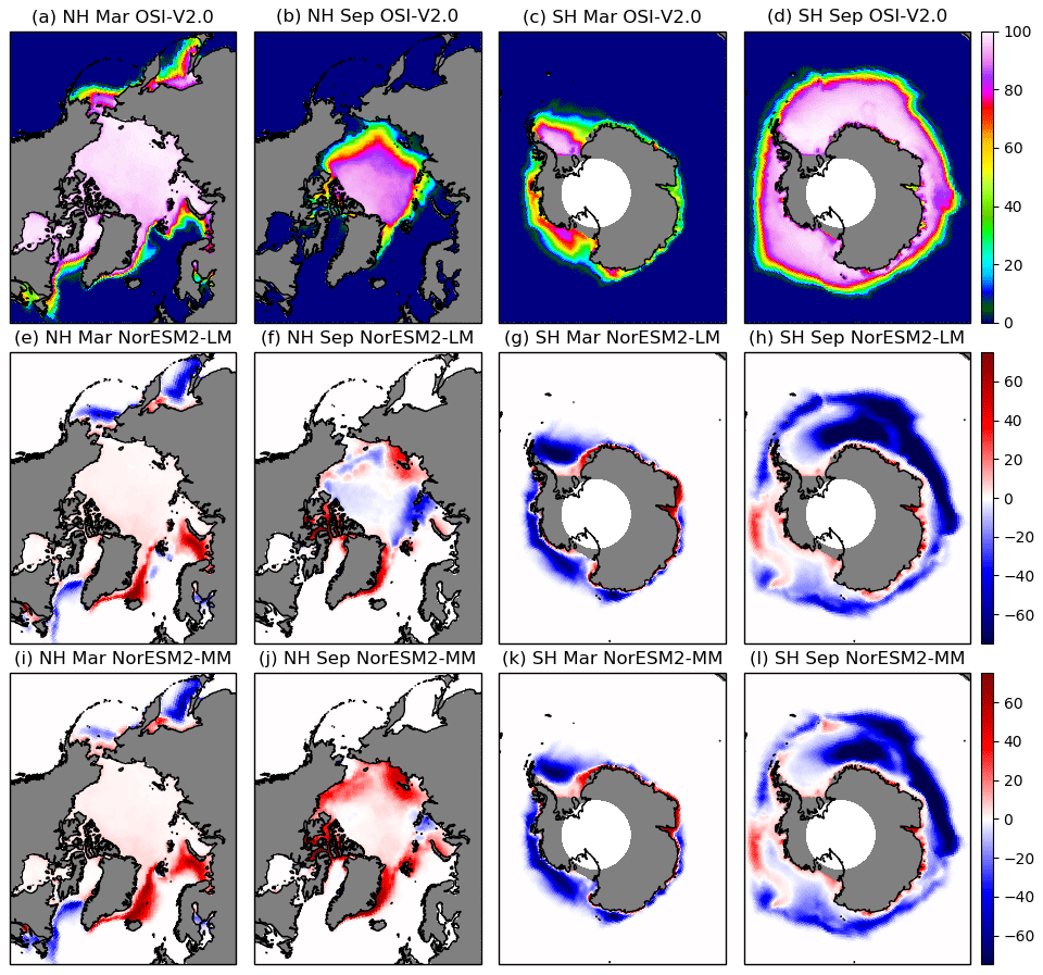
Figure 12Sea-ice concentration from OSISAF observations (OSI-V2.0; Lavergne et al., 2019) in March (a, c) and September (b, d) for the Northern Hemisphere (a, b) and Southern Hemisphere (c, d). Differences between model ensemble means and observations for the respective hemisphere and months are shown for NorESM2-LM (e–h), and NorESM2-MM (i–l). Model and observations are monthly means for the period 1980–2009. Units are %.
During summer, the distribution of sea ice in NorESM2-LM (Fig. 12f) seems to be more variable. Apart from the persistent, positive bias in the East Greenland Current, the regional biases within the Arctic Ocean are more likely due to interannual variability and the effect that the observations show a larger downward trend than the model.
NorESM2-MM (Fig. 12j) shows too much sea ice in the central Arctic in September. In general, the model is colder in the Arctic than NorESM2-LM (Fig. 14), and it has thicker sea ice in the Arctic Ocean. The Northern Hemisphere sea-ice volume in NorESM2-MM is 21 % (36 %) larger in March (September) compared with the NorESM2-LM (not shown). The smaller seasonal cycle in ice area (Fig. 13) and volume is consistent with a thicker sea-ice cover in NorESM2-MM, both due to less winter growth because of increased insulation and less summer melt due to higher albedo. The situation encountered in NorESM2-MM is similar to the results from NorESM1-M (Bentsen et al., 2013) and NorESM1-Happi (Graff et al., 2019). These models simulate ice cover that is too thick, with the reduction in the Northern Hemisphere summer ice area being too slow.
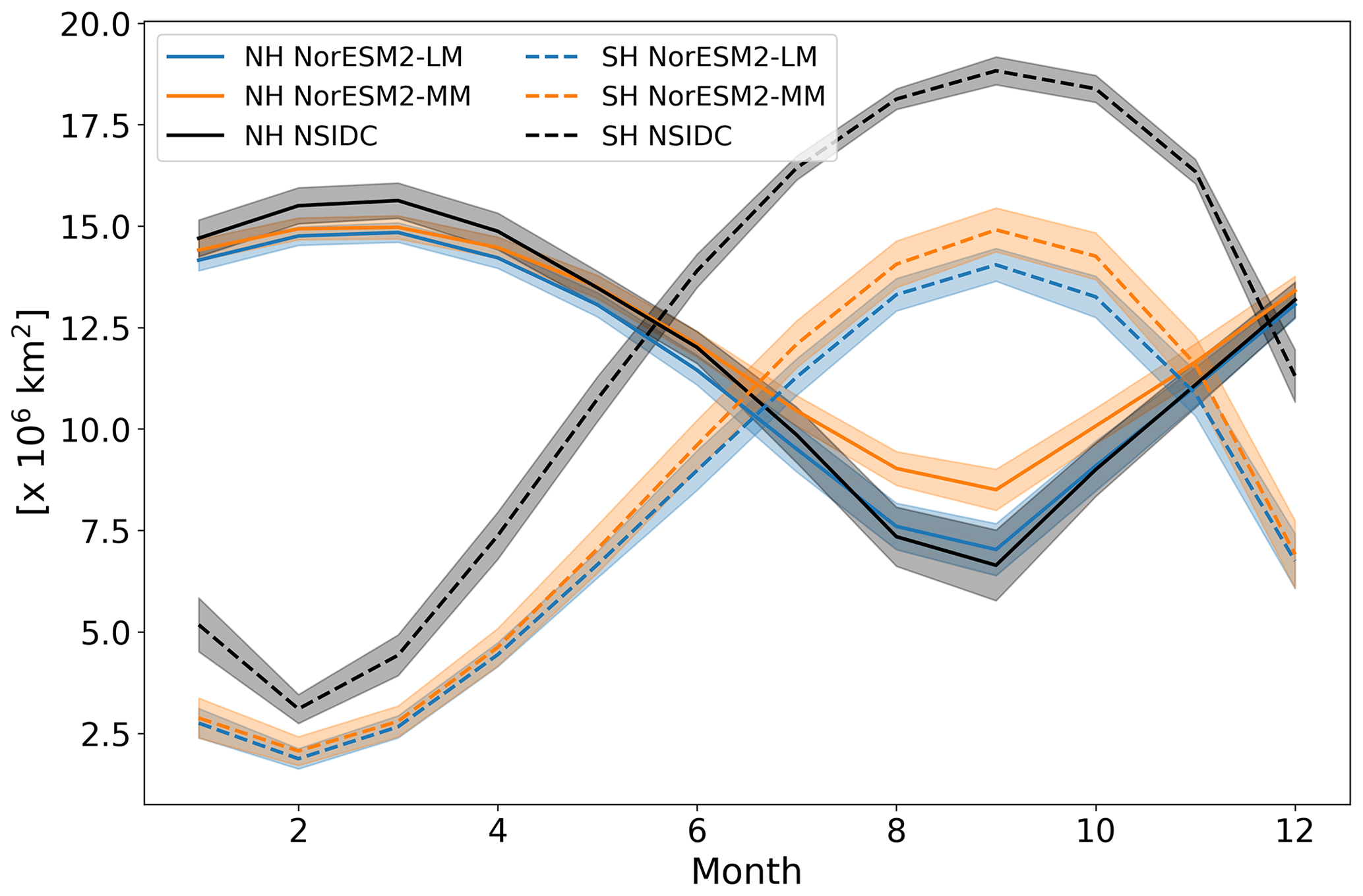
Figure 13Northern Hemisphere (NH) and Southern Hemisphere (SH) seasonal cycles of sea-ice extent in the first historical member from NorESM2-LM and from NorESM2-MM averaged over the years 1980–2009 and compared to observations from NSIDC. Shaded areas show interannual variation as standard deviation. Units are 106 km2.
The winter sea-ice area and extent is too low in the Southern Ocean in NorESM2 as seen in Figs. 13 and 12g–h, k–l. Winter area in September is around 4 million km2 too small. The largest bias is found in the Atlantic–Indian sector. This bias seems to be associated with the warm bias in the ocean model, and the too-warm Antarctic Intermediate Water (AAIW). The exact reason for this problem is not known, but the warm bias in AAIW is also evident in the OMIP simulations (not shown). However, these uncoupled simulations have a reasonable representation of the upper ocean temperature and the winter sea-ice extent that are most likely due to the inherent relaxation towards observed atmospheric temperatures in those experiments. With the interactive atmosphere, these problems increase.
5.3 Atmospheric temperature and winds
In terms of mean surface temperatures, NorESM2 is a warmer model than its preceding versions. The global-mean near-surface temperature (Fig. 14) in NorESM1-M and NorESM1-Happi is generally too low with global-mean biases of −0.76 and −1.08 K (see legends above panels in Fig. 14). NorESM2-MM is closer to the reanalysis with a global-mean bias of −0.19 K. Regionally, cold biases are mostly found in the polar regions and over the subtropical oceans. Warm biases are found over the Southern Ocean, North American continent and in central Eurasia. NorESM2-LM (Fig. 14a) is warmer still, and overestimates the near-surface temperatures in the Arctic and in the global mean, with a bias of 0.43 K. NorESM2-MM has the best overall performance also in terms of the global-mean RMSE, with 1.35 K compared to 1.62 K for NorESM2-LM, and 1.83 K for NorESM1-Happi, and 1.86 K for NorESM1-M (see Fig. 14).
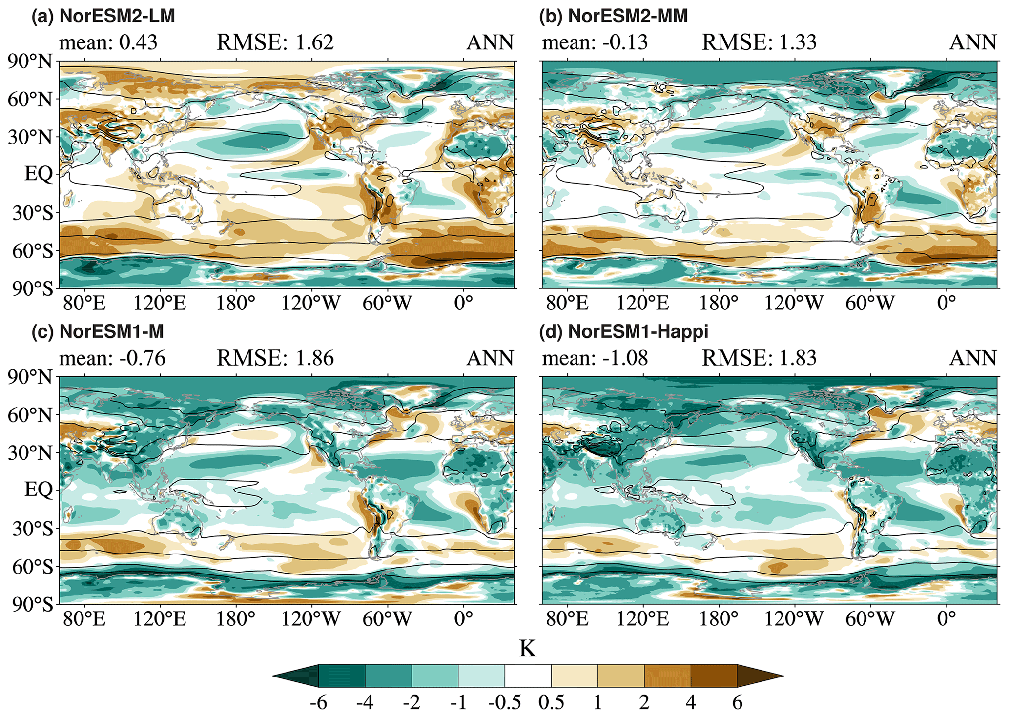
Figure 14Annual-mean ensemble-mean model bias for near-surface temperature (colours) shown with the present-day model climatology (solid black contours; values from 260 K to 300 K by 10 K) from NorESM2-LM (a; years 1980–2009), NorESM2-MM (b; years 1980–2009), NorESM1-M (c; years 1976–2005), and NorESM1-Happi (d; years 1976–2005). The bias is taken with respect to ERA-Interim (years 1979–2008 for NorESM1-M/Happi and 1980–2009 for NorESM2-LM/MM). Units are K.
Temperature biases are reduced in NorESM2 compared to NorESM1, not only near the surface but also and especially in the middle and upper troposphere (Fig. 15). Tropospheric air temperatures tend to be systematically cold in all versions of both CESM and NorESM. NorESM2 has a reduced cold bias compared to NorESM1 particularly in the tropics and subtropics. This is mostly a consequence of the changes made to the cumulus convection scheme (Toniazzo, 2020). The higher tropical SSTs in NorESM2-LM compared to NorESM2-MM lead to a reduced cold tropospheric tropical bias; however, persistent cold midlatitude and high-latitude biases imply an excessive meridional temperature gradient. By contrast, NorESM2-MM shows improvements at all latitudes.

Figure 15Annual-mean ensemble-mean model bias for temperature (colours) shown with the present-day model climatology (solid black contours; values from 210 K to 285 K by 15 K) from NorESM2-LM (a; years 1980–2009), NorESM2-MM (b; years 1980–2009), NorESM1-M (c; years 1976–2005), and NorESM1-Happi (d; years 1976–2005). Three ensemble members are used for all model versions. The bias is taken with respect to ERA-Interim (years 1979–2008 for NorESM1-M/Happi and 1980–2009 for NorESM2-LM/MM). Units are K.
The stronger cool tropospheric and warm surface tropical bias of NorESM2-LM compared with NorESM2-MM is in line with the behaviour of both NorESM1 and CESM2. The systematic difference between the two atmosphere resolutions is also consistent between coupled and AMIP simulations, with CAM-Nor significantly cooler at 2∘ resolution than at 1∘ resolution for the same SSTs and the same physics parameters. At the same time, tropospheric specific humidity (and, a fortiori, relative humidity) is higher. Both lead to higher corresponding RESTOM. The ultimate cause of this systematic dependence of the simulated climatology on the resolution of the atmosphere model is not known. There may be a sensitivity of the convection parameterisation to the grid-scale variability of near-surface air parameters and to boundary-layer stability. Another possibility is a resolution dependence of cloud microphysics and the efficiency of stratiform precipitation. Liquid water path (LWP) and column precipitable water appear almost uniformly higher in CAM-Nor at 2∘ resolution than at 1∘ resolution.
All four configurations (NorESM2-MM, NorESM2-LM, NorESM1-Happi, and NorESM1-M) tend to produce tropospheric westerly biases in zonal-mean zonal winds (Fig. 16). At tropical and subtropical latitudes, these are more widespread in NorESM2 than NorESM1-M and NorESM1-Happi. Surface wind biases, which by contrast tend to be easterly, are reduced. At higher latitudes, all models tend to have westerly biases on the poleward side of the subpolar surface jet (between 50 and 60∘) in both hemispheres. The overestimation on the poleward flank is generally more pronounced in NorESM2 than in NorESM1. Comparing NorESM1-M to NorESM1-Happi and NorESM2-LM to NorESM2-MM, the biases in the zonal wind tend to be ameliorated with increased resolution. The differences in the tropics between NorESM2 and its predecessors are in part attributable to the enforcement of conservation of atmospheric global angular or rotational momentum in NorESM2 (Toniazzo et al., 2020). In all versions, in common with CAM6/CESM2, there is accumulation of westerly momentum near the model lid, where it is insufficiently damped.
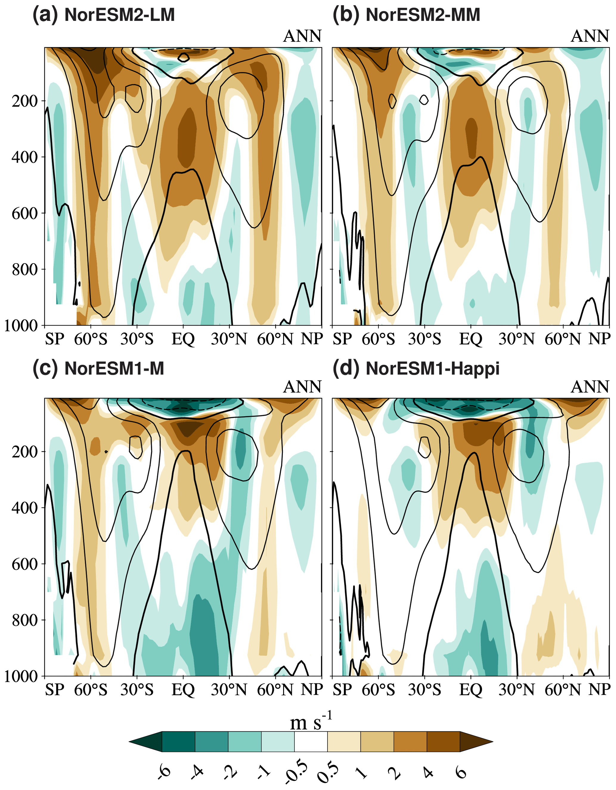
Figure 16Annual-mean ensemble-mean model bias for the zonal wind (colours) shown with the present-day model climatology (solid black contours show positive values and dashed negative values; contour interval is 10 m s−1; zero contour is extra thick) from NorESM2-LM (a; years 1980–2009), NorESM2-MM (b; years 1980–2009), NorESM1-M (c; years 1976–2005), and NorESM1-Happi (d; years 1976–2005). Three ensemble members are used for all model versions. The bias is taken with respect to ERA-Interim (years 1979–2008 for NorESM1-M/Happi and 1980–2009 for NorESM2-LM/MM). Units are m s−1.
5.4 Extratropical storm tracks
Extratropical storm tracks can be defined as regions of storminess associated with cyclogenesis, cyclone development, and cyclolysis which take place in the baroclinic zones between the subtropics and polar regions. They are important features at midlatitudes and high latitudes as they are responsible for eddy transport of heat and momentum between low and high latitudes, and associated with potentially high-impact weather such as heavy precipitation and strong winds. Here, we diagnose storm-track activity by applying a bandpass filter to retain fluctuations in the geopotential height field at 500 hPa with periodicity corresponding to that of baroclinic waves, that is, between 2.5 and 6 d (Blackmon, 1976; Blackmon et al., 1977). The variability of the bandpass-filtered field is dominated by propagating low-pressure and high-pressure systems, and the storm tracks can be defined as geographically localised maxima in bandpass-filtered variability (Blackmon, 1976; Blackmon et al., 1977; Chang et al., 2002; Graff and LaCasce, 2012).
The climatological winter storm tracks are shown as the solid black contours in Fig. 17. There are two maxima in the Northern Hemisphere: one over the North Atlantic and one over the North Pacific. The colours show the bias with respect to ERA-Interim (Dee et al., 2011). In NorESM1-M, storm-track activity is underestimated in both storm-track regions. In particular, the North Atlantic storm track is overly zonal with too little activity on the equatorward side of the climatological maximum as well as over the Norwegian and Barents seas (Iversen et al., 2013; Graff et al., 2019). The magnitude of the bias is reduced in NorESM1-Happi compared to NorESM1-M in both storm-track regions. This is likely associated with the increased resolution in the atmosphere and land components (1∘ in NorESM1-Happi versus 2∘ in NorESM1-M).
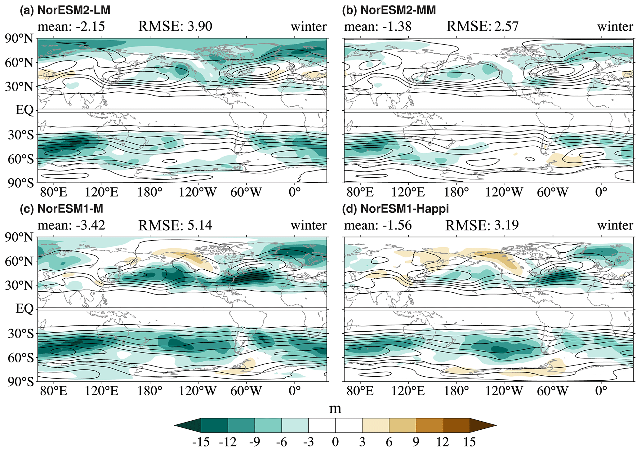
Figure 17Ensemble-mean model bias for the extratropical storm tracks in terms of bandpass-filtered variability (colours) shown with the present-day model climatology (solid black contours; values from 8 m with intervals of 8 m) for NorESM2-LM (a), NorESM2-MM (b), NorESM1-M (c), and NorESM1-Happi (d). Panels show the winter season for both hemispheres (DJF for the NH and JJA for the SH). The storm tracks are plotted in terms of the standard deviation of the bandpass-filtered geopotential height field at 500 hPa (Z500). The model data are taken from the CMIP6 historical members for NorESM2-LM (three members) and NorESM2-MM (three members) for the years 1980–2009 and from the CMIP5 historical members for NorESM1-M (three members) and NorESM1-Happi (three members) for the years 1976–2005. The bias is taken with respect to ERA-Interim (years 1980–2009 for NorESM2-LM/MM and 1979–2008 for NorESM1-M/Happi). Units are metres.
Similar improvements are seen when comparing NorESM2-LM and NorESM2-MM. Both versions of NorESM2 are, furthermore, better able to simulate the North Atlantic storm track with the size of the negative bias on its equatorward side being reduced. Overall, NorESM2-MM displays the smallest biases in Northern Hemisphere storm-track activity out of the four models. There remains, however, too little activity over the Norwegian Sea with extension into the Barents Sea.
In the Southern Hemisphere, the climatological winter storm track surrounds Antarctica with the largest variability occurring over the Indian Ocean (Fig. 17). Storm-track activity is generally too weak on the equatorward side, with the largest biases being located over the Indian Ocean, close to the storm-track maximum. As in the Northern Hemisphere, the largest biases are found in NorESM1-M and the smallest biases in NorESM2-MM.
While the bandpass-filter approach yields a measure of storm-track activity, it cannot be used to isolate the individual cyclone centres. To further assess the robustness of the improvements between NorESM2-LM and NorESM2-MM, we therefore also consider results from the cyclone detection algorithm described in Wernli and Schwierz (2006). The method detects cyclones as minima in the sea-level pressure fields and sets the perimeter as the outermost closed sea-level pressure contour. The storm tracks are then seen as maxima in the local frequency of occurrence of surface cyclones, i.e. the fraction of time when cyclones are present in a given point (Fig. 18a–b).
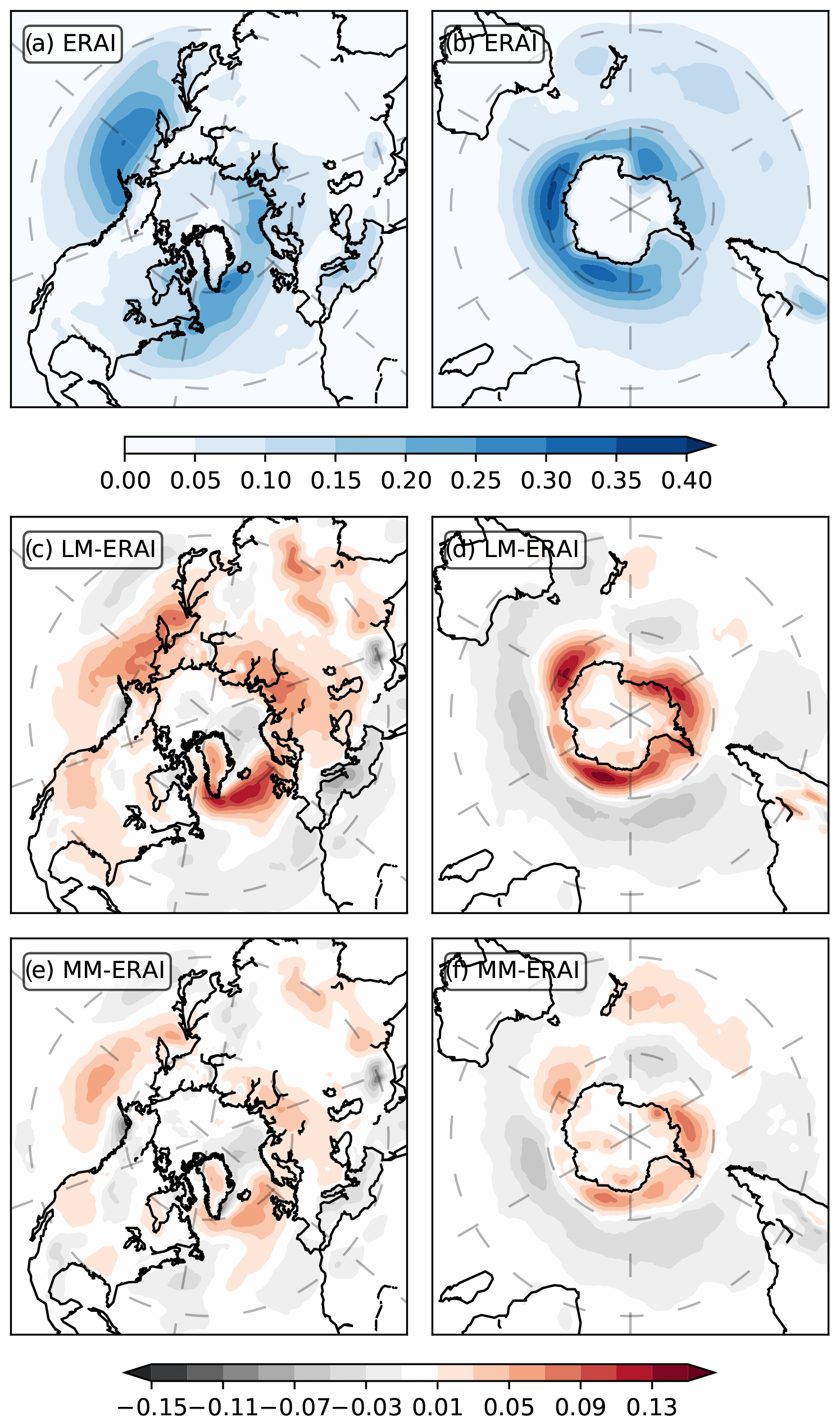
Figure 18Frequency of occurrence (the unitless numbers give the fraction of the time when cyclones are present) of extratropical surface cyclones for the Northern Hemisphere (a, c, e) and Southern Hemisphere (b, d, f) storm tracks during the respective winter seasons (DJF in the Northern Hemisphere and JJA in the Southern Hemisphere). The figure shows the ERA-Interim climatology (a–b) and the ensemble-mean bias with respect to ERA-Interim for NorESM2-LM (c–d) and NorESM2-MM (e–f). The data are taken from the years 1980–2009. Three members are used for both versions of NorESM.
As for the bandpass-filter approach, the cyclone detection shows a clear reduction in the bias between NorESM2-LM and NorESM2-MM, which is likely to be associated with the higher horizontal resolution in the atmosphere and land components. The cyclone occurrence is underestimated on the equatorward side of the North Pacific and Southern Hemisphere storm tracks and overestimated on the poleward side. Over the North Atlantic, the cyclone occurrence is underestimated on the equatorward side of the storm track and over the Norwegian Sea extending into the Barents Sea, and overestimated between the British Isles and Greenland. The magnitude of the bias is clearly reduced in all regions in NorESM2-MM, with the improvement being particularly evident in the regions where the cyclone occurrence is overestimated.
Note that both the climatology and the biases should be expected to differ somewhat between the two approaches considered here because they capture different aspects of the storm tracks. The bandpass-filter approach does not distinguish between cyclones and anti-cyclones, and is dominated by growing and propagating baroclinic waves (Blackmon et al., 1977). The cyclone occurrence reflects the regions where cyclone centres are identified most frequently, and is, for instance, more sensitive to systems that are slowly moving or too long lived.
5.5 Clouds and forcing
Table 4 gives an overview of major forcing fluxes in NorESM2 compared to NorESM1 and observational estimates. Despite the large differences in physics and tuning, the overall numbers for top-of-the-atmosphere fluxes and forcings are very similar to the numbers found in NorESM1-Happi and are generally within the observational range. There is however a slightly stronger negative bias in clear-sky LW flux and long-wave cloud forcing. The latter is an unfortunate consequence of the tuning of high clouds in the model implemented in order to increase the outgoing long-wave radiation. As seen from the upward LW flux estimate, the outgoing long-wave radiation is still within the estimate from satellite retrievals. SWCF values are very similar to the values of NorESM1-Happi and within the observational range. This number hides, however, a major weakness in NorESM1 stratiform cloud parameterisation which underestimated the cloud cover and compensated this by overestimating the cloud liquid water.
Table 3 Summary of Carbon fluxes and stocks. Fluxes of gross primary production (GPP; Pg C yr−1), and soil and vegetation carbon stocks (Pg C). Data are averaged over the period 1995–2014 for NorESM2 (MM and LM) and 1982–2005 for NorESM1 (Tjiputra et al., 2013). Observational data for GPP are from FLUXNET-MTE (Jung et al., 2011), for soil C from the Harmonized World Soil Database (Fao/Iiasa/Isric/Isscas/Jrc, 2012) and veg. C from GEOCARBON project (Avitabile et al., 2016; Santoro et al., 2015), are all available from http://ILAMB.org (last access: 8 June 2020).
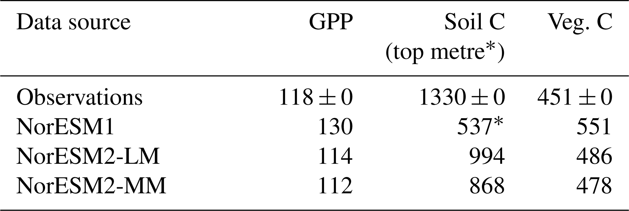
* Except for NorESM1, where soil carbon includes the full soil column.
Table 4 Global and annual means from the historical (years 1980–2009) simulations for NorESM2-MM and NorESM2-LM (three-member ensemble average). Values from reanalysis data or observations (references in the last column). The NorESM values are adjusted to compensate for the slight deviation between the top of the model atmosphere (abbreviated to TOA) and the top of the atmosphere as seen from satellites (Collins et al., 2006; TOASAT in this table).
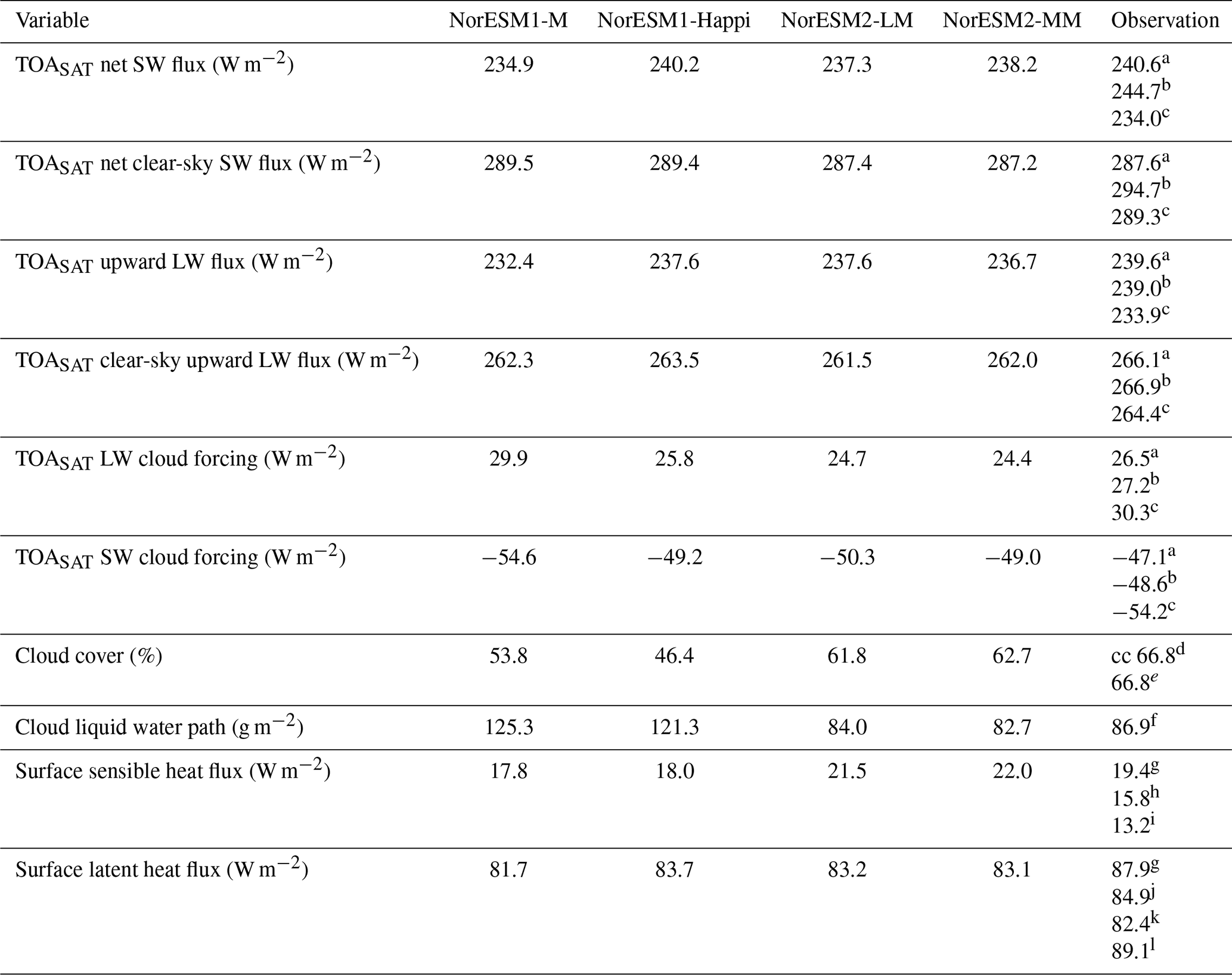
a CRES-EBAF (Loeb et al., 2005, 2009, 2012). b CRES (Loeb et al., 2005, 2009, 2012). c ERBE (Harrison et al., 1990; Kiehl and Trenberth, 1997). d ISCCP (Rossow and Schiffer, 1999; Rossow and Dueñas, 2004). e CLOUDSAT (L'Ecuyer et al., 2008). f (O’Dell et al., 2008). g JRA25 (Onogi et al., 2007). h NCEP (Kanamitsu et al., 2002). i LARYEA (Large and Yeager, 2004). j ECMWF (Trenberth et al., 2011). k ERA40 (Uppala et al., 2005). l WHOI (Yu and Weller, 2007; Yu et al., 2008).
The major updates in cloud physics from CAM4 to CAM6 (Bogenschutz et al., 2018) improved the cloud cover, and the cloud liquid water path is now quite close to the observational estimate. The global cloud cover is still slightly lower than observed (Table 4). This is partly connected to the tuning in NorESM2. Prior to the tuning, the modelled cloud cover was higher than 70 %. As seen from Fig. S5 in the Supplement, the cloud cover underestimate is most pronounced in the tropics and subtropics in both hemispheres, while there is good agreement around the extratropical storm-track regions and an overestimate in the high Arctic. Before the tuning (not shown), there was no bias at the low latitudes.
The modelled liquid water path seems to have a systematic bias towards low values at low latitudes and high values in the extratropics. Possible connections between cloud cover biases and the hydrological cycle are discussed in the next section.
5.6 Precipitation and hydrological cycle
The bias in the annual-mean total precipitation rate is shown in Fig. 19 for the two versions of NorESM1 and NorESM2 relative to data from the Global Precipitation Climatology Project (GPCP; Adler et al., 2003). While the bias of the global-mean average is not systematically reduced between NorESM1 and NorESM2, there is a reduced RMSE, indicating that there is less cancellation between positive and negative biases in the global mean.
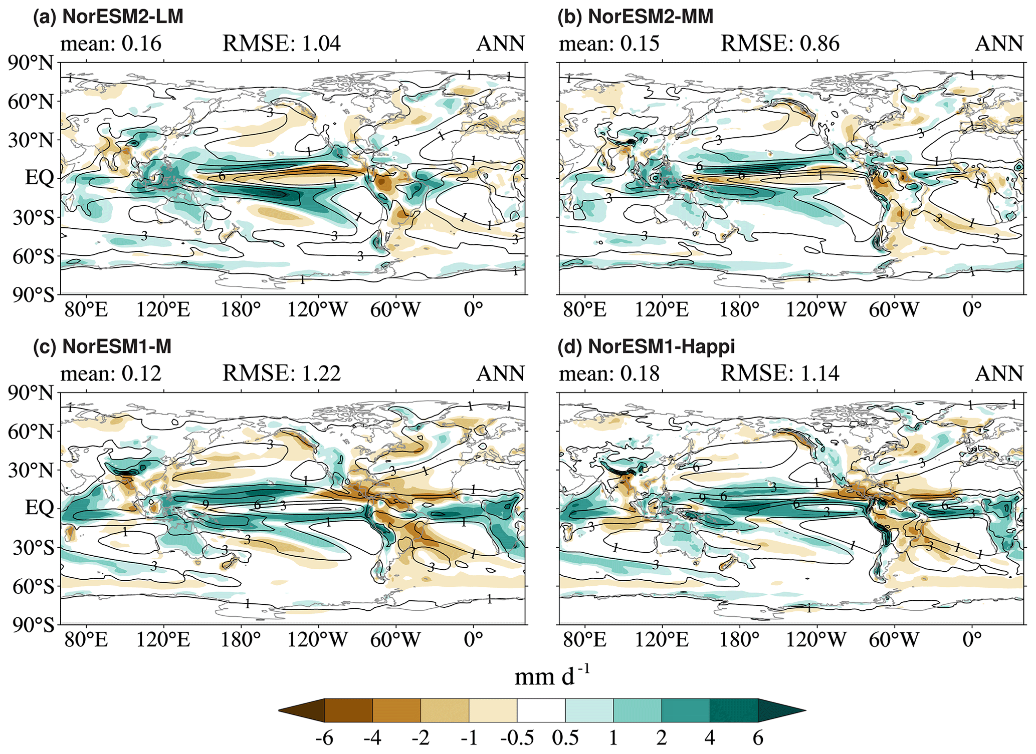
Figure 19Annual-mean ensemble-mean model bias for total precipitation rate (colours) shown with the present-day model climatology (solid black contours; values from 1 by 2 mm d−1) from NorESM2-LM (a; years 1980–2009), NorESM2-MM (b; years 1980–2009), NorESM1-M (c; years 1976–2005), and NorESM1-Happi (d; years 1976–2005). Three ensemble members are used for all model versions. The bias is taken with respect to GPCP (years 1979–2008 for NorESM1-M/Happi and 1980–2009 for NorESM2-LM/MM). Units are mm d−1.
The reduction of the RMSE is also seen when considering the four seasons separately in Fig. S6 in the Supplement along with climatology from the GPCP. The evaluation of the mean bias, RMSE, and correlation included in the bottom left corner of each panel shows that RMSE and correlation have improved in NorESM2 compared to NorESM1 for all seasons. While the overall wet bias has increased slightly, mostly due to strong biases over the Pacific Ocean, there are regions with a large reduction in mean bias. This is especially pronounced over Africa and equatorial Atlantic Ocean. The largest improvement compared to NorESM1-M is seen for NorESM2-MM during northern hemisphere winter, when all three metrics (bias, RMSE, and correlation) consistently indicate higher skill.
As a measure of interannual variability, the standard deviation of monthly means for each season was calculated. The differences compared to GPCP are presented in Fig. S7 in the Supplement. While NorESM1 slightly underestimates the precipitation variability, it is somewhat too high in NorESM2, with the magnitude of the bias being larger in all seasons. NorESM2-MM improves RMSE of precipitation variability in all seasons except northern hemisphere autumn. As also seen for the mean climatology in Fig. S6 in the Supplement, the correlation has improved for all seasons in both NorESM2-LM and MM.
The hydrological cycle (or cycling of fresh water) is of major importance for the climate system. Global means of precipitation and evaporation can serve as integrated measures of the properties of many processes in an ESM. Results presented in Table 5 indicate that the intensity of hydrological cycle, as measured by evaporation, in NorESM2 is about 1.4 % larger globally (4.9 % over oceans) than in NorESM1-M. This is also manifested in the positive precipitation biases in Fig. 19. While the values in Table 5 for NorESM2 are higher than for GPCP, they are closer to results from ERA-Interim calculated by Trenberth et al. (2011). Although NorESM1-Happi has the highest precipitation globally, NorESM2 has the highest precipitation over ocean, suggesting a larger recycling of oceanic water vapour and a lower fraction transported from oceans to continents (measured by E−P over oceans). The overestimated evaporation over oceans is likely linked to the underestimated cloudiness in the tropics and subtropics (Fig. S5 in the Supplement). Solar radiation over subtropical ocean regions is an important driver of evaporation. The net moisture transport from oceans to continents is nevertheless smaller in NorESM2 than in NorESM1, consistent with more clouds in the extratropics and more marine precipitation in NorESM2. This analysis is only preliminary, however, and needs more in-depth studies which is out of scope of the present paper.
Table 5 Evaporation (E) and precipitation (P) for different historical NorESM simulations and reference datasets. Units are in thousands of cubic kilometres of water per year. The years used are 1980–2009, except for NorESM1-Happi (1976–2005) which is from Graff et al. (2019), and the last two lines (2002–2008) which are from Trenberth et al. (2011).
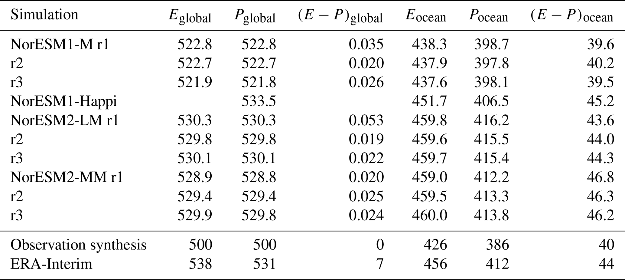
In NorESM2, a closed hydrological cycle is present, with the difference between evaporation and precipitation being close to zero in the long-term average at equilibrium. In NorESM2-MM, the discrepancy is slightly improved to 0.023 km3 yr−1, whereas it is 0.027 km3 yr−1 in NorESM1-M and 0.031 km3 yr−1 in NorESM2-LM (all values are means from members 1–3).
5.7 Northern Hemisphere blocking
While storm tracks are closely tied to precipitation, atmospheric blocking is associated with persistent anti-cyclones that inhibit precipitation for timescales up to several weeks. To diagnose blocking, we apply the variational Tibaldi and Molteni (vTM) index (Tibaldi and Molteni, 1990; Pelly and Hoskins, 2003; Iversen et al., 2013; Graff et al., 2019). Blocks are identified when there is persistent reversal of the 500 hPa geopotential height field around a central latitude that last for at least 5 d and cover at least 7.5 consecutive longitudes. The central longitude varies with the position of the maximum in the Northern Hemisphere climatological storm track.
The seasonal blocking frequency is mostly underestimated over the North Atlantic and in Europe in the four versions of NorESM (Fig. 20), particularly during winter (DJF). During spring (MAM), NorESM2-MM is closest to the reanalysis, while during summer (JJA) and autumn (SON), NorESM1-Happi performs best in these regions. While NorESM1 tends to overestimate the blocking frequency over the Pacific, NorESM2 generally lies closer to the reanalysis in that sector. Consider, for instance, the region between 120 and 180∘ E during summer, or the region between 130 and 90∘ W during winter. In summary, although the use of 30 years from ERA-Interim for verification may not be fully representative of blocking climatology, the representation of NH blocking continues to be a challenge in NorESM and in particular over the Atlantic–European sector in winter.
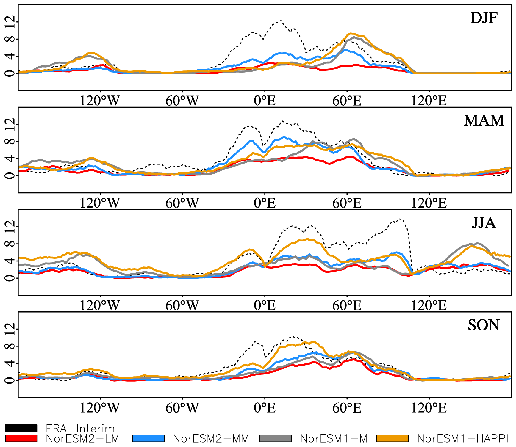
Figure 20Ensemble-mean seasonal blocking frequency in the Northern Hemisphere for ERA-Interim (stippled black line; years 1980–2009), NorESM2-LM (solid red line; years 1980–2009), NorESM2-MM (blue line; years 1980–2009), NorESM1-M (grey line; years 1976–2005), and NorESM1-Happi (yellow line; years 1976–2005). The model data are taken from the CMIP6 historical members for NorESM2-LM (three members) and NorESM2-MM (three members) and from the CMIP5 historical members for NorESM1-M (three members) and NorESM1-Happi (three members). The blocking frequency is computed using the vTM index (Tibaldi and Molteni, 1990; Pelly and Hoskins, 2003; Iversen et al., 2013; Graff et al., 2019). Units are %.
5.8 Madden–Julian Oscillation
In the tropical atmosphere, the Madden–Julian Oscillation (MJO) is the dominant mode of variability on timescales between 30 and 90 d (Madden and Julian, 1971; Zhang, 2005). The MJO is characterised by a meridional dipole of convective precipitation anomalies along the Equator, that slowly propagates eastwards and interacts with a number of other circulation features such as El Niño events (Hendon et al., 2007), the Indian summer monsoon (Annamalai and Slingo, 2001), tropical cyclones (Liebmann et al., 1994), and even the North Atlantic Oscillation and extratropical variability (Cassou, 2009).
The MJO is characterised by a specific feature in wavenumber–frequency spectrum of equatorial 850 hPa zonal wind (U850) and outgoing long-wave radiation (OLR; Waliser et al., 2009), associated with wavenumbers 1–3, a maximum at wavenumber 1, and periods between 30 and 80 d. NorESM2-LM and NorESM2-MM possess this mode in U850 spectra (Fig. S8 in the Supplement), but its spread in wavenumber is too narrow and its spread in frequency too wide. Furthermore, OLR variability is too weak, and the mode appears preferentially as a stationary oscillation in the Indian Ocean sector, with too little zonal and meridional propagation (Fig. S9 in the Supplement). The relationship between zonal winds and precipitation anomalies, with the former in quadrature with respect to the latter, is similar in the simulations and in observations. In NorESM2-MM (Fig. S9c in the Supplement), however, the anomalies appear to be generally too weak. Composite plots of MJO events (not shown) indicate a tendency in both model versions to generate westward-propagating convective anomalies, which may weaken activity in the MJO region of the spectrum. The ability of the simulated MJO mode to propagate eastwards as observed appears to be sensitive to the distribution of tropical SSTs in both CESM2 and NorESM2 (Richard Neale, personal communication, 2020; Toniazzo, 2020).
5.9 El Niño–Southern Oscillation
The coupled model internally generates a self-sustained ENSO mode with spatial and temporal characteristics similar to observations. (The time series of NINO3.4 SST anomalies are shown in Fig. S10 in the Supplement, alongside the observed one.) The ENSO modes in LM and MM model versions are very similar in magnitude (Figs. 22–23), spatial pattern (Fig. 23), and spectral power distribution in frequency space (Fig. 21). ENSO SST anomalies are very large compared to observations (with a NINO3.4 anomaly greater than 2.5 ∘C in the average El Niño event, compared with 1.5 ∘C in observations), and they tend to peak early in the season, i.e. between November and December instead of between December and January as observed (Fig. 22a). The early peak and termination may be partly attributable to weak zonal wind-stress anomalies over the equatorial region, which also peak early, notwithstanding a robust response in equatorial precipitation (Fig. 22b, c). Such weak surface wind response may be caused by the general displacement, with respect to observations, of the maximum of climatological precipitation north of the Equator along the Pacific ITCZ. Especially in MM, precipitation anomalies also have their maximum north of the Equator (Fig. 23b), which tends to result in weaker equatorial anomalous westerlies. A second origin of the early simulated El Niño SST peak may however also be found in the early rapid demise of positive thermocline depth anomalies in the NINO3 region during El Niño events, which is seen also in OMIP1 and OMIP2 simulations forced with prescribed wind stress (Fig. 22d). Given the weak coupled wind stress and thermocline activity, the large SST anomalies may be partly the result of insufficient surface damping by the action of anomalous surface heat fluxes.
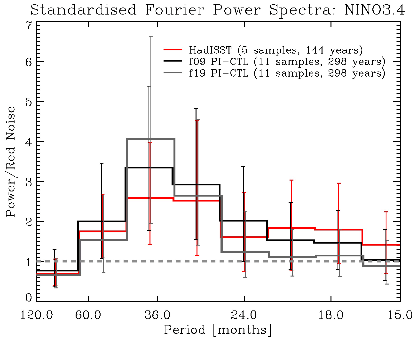
Figure 21Frequency analysis of El Niño events in NorESM2-MM (f09) and NorESM2-LM (f19) and the Hadley Centre Sea Ice and Sea Surface Temperature dataset (HadISST) v1.1 (Rayner et al., 2003) observed data. Fourier power spectra of NINO3.4 anomalies, normalised to AR1 red-noise model for each (using bootstrapping, 1000 samples).
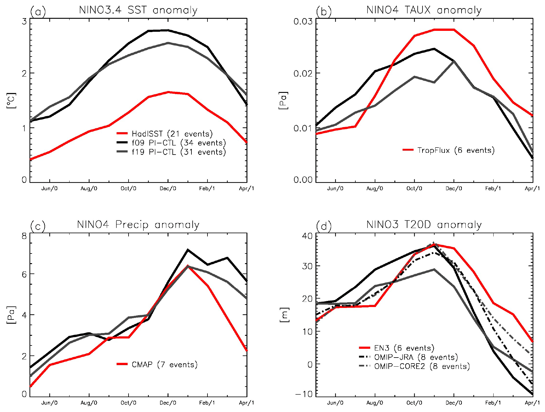
Figure 22El Niño monthly mean composite anomalies averaged over various NINO regions (see the legend at the top of each panel) for SST, zonal wind stress, precipitation, and 20 ∘C isotherm depth in the Equatorial Pacific. The composite El Niño event is obtained by averaging a number of years during which the occurrence of El Niño is diagnosed based on NINO3.4 anomalies. The selection criteria are on magnitude (1.5 standard deviations), duration (3 months), seasonality (peak between November and January), and phase (no preceding El Niño and a following La Niña). Year 0 indicates the year during which the event develops. For the observations, SSTs are from HadISST (Rayner et al., 2003), wind stress is from TropFlux (Praveen Kumar et al., 2012), precipitation is from CMAP (Xie and Arkin, 1997), and the 20 ∘C isotherm depth is obtained from the EN3 dataset (Guinehut et al., 2009).
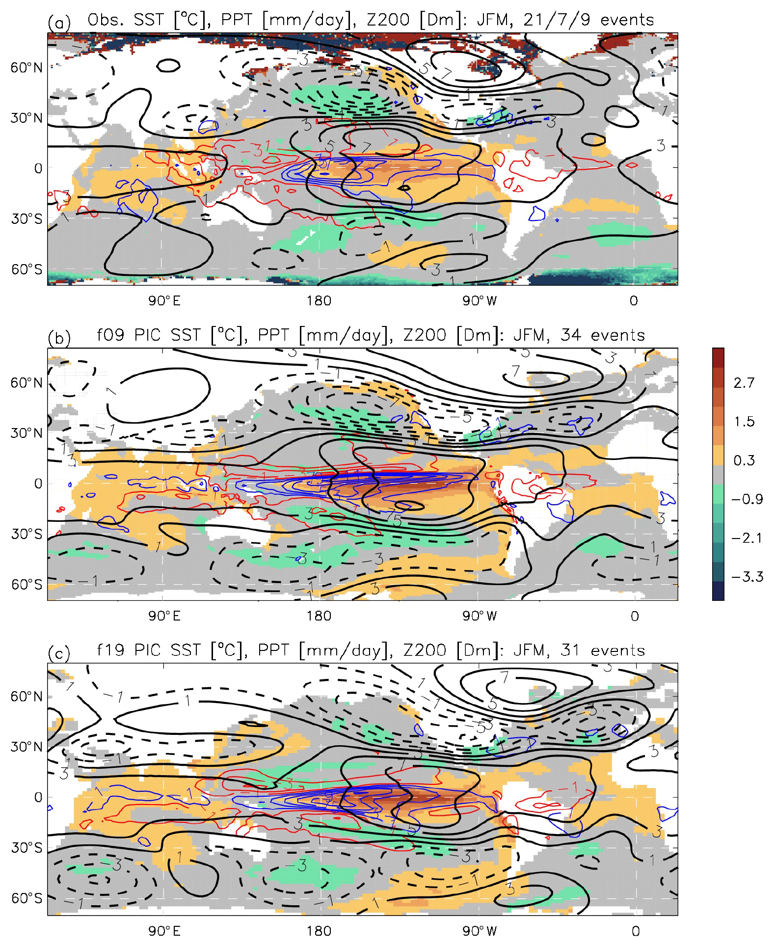
Figure 23El Niño JFM composite anomalies from observations (a), NorESM2-MM (b), and NorESM2-LM (c). Colour-filled contour levels denote SST anomalies (contour levels indicated in the legend on the right side of panel b), precipitation anomalies (coloured line contours, red for negative values and blue for positive values; interval 2 mm d−1), and geopotential height anomalies at 200 hPa (black and white contour lines, solid for positive and stippled for negative values; interval 20 m). The composites are defined as for Fig. 22 (see the caption to that figure).
Correlation analysis shows that indeed over the eastern equatorial Pacific the model tends to generate positive downward net short-wave radiative flux anomalies when SST anomalies are positive, in contrast to observations. This might also explain the growth of positive SST anomalies in the NINO3.4 region early during El Niño events, even before positive 20 ∘C isotherm depth anomalies have fully reached the area, and the long persistence of both SST and precipitation anomalies in the later stages of El Niño events. The model climatological bias of a pronounced double ITCZ, with strong ITCZ precipitation away from the Equator and a dry, cold equatorial region dominated by marine stratocumulus, rather than trade-cumulus cloud in the eastern Pacific, probably contributes to this behaviour. Toniazzo (2020) shows that changes in the convection scheme that were made in order to mitigate the tropospheric cold bias and the positive TOA net residual have contributed to this error. Off-equatorial precipitation tends to couple less effectively with eastward-propagating equatorial modes (see also the previous section and Fig. S9). Westward propagation is also evident in the model's ENSO during the phase change from El Niño to La Niña. In spite of such shortcomings, ENSO-related variability in NorESM2 is generally similar to the observed one. In particular, NINO3.4 spectra in the two model versions and in observations are formally indistinguishable (Fig. 21). The simulated composite El Niño SST, precipitation, and geopotential height anomalies have good global pattern correlations with the observed composite El Niño anomalies (Fig. S11 in the Supplement), indicating that the simulated ENSO adds important and useful features to the climatology simulated by the model. Particularly prominent and fairly realistic are teleconnections into both hemispheres during and after ENSO peaks, with a Pacific/North American (PNA) pattern that extends into the storm-track entry region of the western Atlantic, as observed. In this respect, NorESM2-MM validates better than NorESM2-LM, in spite of its equivalent of slightly worse equatorial ENSO biases, probably due to a better overall subtropical and high-latitude atmospheric circulation.
This paper presents and evaluates NorESM2 (the second version of the Norwegian Earth System Model) used for conducting experiments for CMIP6. NorESM2 is based on CESM2 (the second version of the Community Earth System Model) but with several important differences. While the land and sea-ice components are largely the same as in CESM2, NorESM2 has entirely different models for the ocean and ocean biogeochemistry, namely BLOM and iHAMOCC. There are also several differences in the atmosphere model (CAM6-Nor), including a different module for aerosol life cycle, aerosol–radiation–cloud interactions and changes related to the moist energy formulation, deep convection scheme, and angular momentum conservation. Finally, the turbulent air–sea flux calculations are modified and proper time averaging of solar zenith angle in albedo estimation implemented.
We report results from the CMIP6 DECK experiments, including the pre-industrial control, the abrupt quadrupling of CO2 concentration levels, and 1 % increase per year of CO2 concentrations until quadrupling, along with the CMIP6 historical experiments, and the ScenarioMIP tier 1 experiments (SSP1-2.6, SSP2-4.5, SSP3-7.0, and SSP5-8.5). The experiments were all carried out with both the atmospheric medium-resolution version of the model (NorESM2-MM) and a low-resolution version (NorESM2-LM).
The drift over the 500-year pre-industrial control experiment is generally very small for both versions of the model. NorESM2 is slightly less sensitive than its predecessors and at the lower end of the CMIP5 and CMIP6 multi-model mean for both model resolutions (Gjermundsen et al., 2020), with the equilibrium climate sensitivity of 2.5 K estimated using the Gregory method (Gregory et al., 2004).
The historical reconstruction of surface temperatures is similar in both model versions. A significant temperature increase due to enhanced climate forcing is found late in the historical period. Both model versions reach present-day warming levels to within 0.2 ∘C of observed temperatures in 2015. Aerosol forcing may be responsible for the delayed warming in the late 20th century. Aerosol effective radiative forcing reaches levels of −1.5 W m−2 in the period 1970–1980, becoming slightly weaker again in 2014 with a value of −1.36 W m−2 in NorESM2-LM and −1.26 W m−2 in NorESM2-MM.
Under the four scenarios (SSP1-2.6, SSP2-4.5, SSP3-7.0, and SSP5-8.5), the warming in the period 2090–2099 compared to 1850–1879 reaches 1.3, 2.2, 3.0, and 3.9 K in NorESM2-LM, and 1.3, 2.1, 3.1, and 3.9 K in NorESM2-MM, robustly similar in both resolutions.
In particular, NorESM2-LM shows a satisfactory evolution of recent sea-ice area. In NorESM2-LM, an ice-free Arctic Ocean is only avoided in the SSP1-2.6 scenario. NorESM2-MM simulates larger sea-ice area both at present and in future scenarios.
The patterns of some biases seen in the fully coupled simulations considered here are similar in coupled ocean–sea-ice simulations carried out for OMIP and can thus be linked to the ocean model having too-coarse resolution and shortcomings in parameterised processes. NorESM2-LM and MM largely share the same biases in the surface ocean, although the MM version is somewhat closer to the observations. Most of the large-scale biases in the surface ocean are also seen in the subsurface.
Like CESM2, NorESM2 is generally a “cold” model, with an initial deficit in atmospheric long-wave cooling that causes a positive RESTOM and leads to heat gain by the ocean and positive SST biases particularly in the tropics. NorESM2 represents an improvement in this respect compared to NorESM1. This is particularly evident in the tropical and subtropical troposphere (Fig. 15). In addition, the medium-resolution version of the model has more realistic upper-tropospheric meridional temperature gradients and reduced near-surface temperature biases.
The extratropical storm tracks are generally better simulated in NorESM2 than in NorESM1, particularly over the North Atlantic. The storm tracks additionally improve with higher resolution, both in the Northern Hemisphere and Southern Hemisphere.
Several aspects of the modelled cycling of fresh water are improved in NorESM2 compared to NorESM1, including the RMSE and spatial correlation of the bias in the total precipitation rate. The intensity of the hydrological cycle as compared to the observationally based findings of Trenberth et al. (2011) is slightly exaggerated in NorESM2, as it was in NorESM1, consistent with the underestimated cloudiness and thus overestimated solar radiation in the tropics and subtropics. The transport of oceanic water vapour over the continents is smaller in NorESM2 than NorESM1, indicating a slightly too-efficient recycling of oceanic water vapour associated with overestimated oceanic precipitation and higher cloudiness in the extratropics.
The seasonal blocking frequency in the Northern Hemisphere is especially underestimated over the Atlantic–European sector during winter (DJF) by NorESM2. During spring (MAM), NorESM2-MM is closest to the reanalysis, while during summer (JJA) and autumn (SON), NorESM1-Happi performs best in these regions. While NorESM1 tends to overestimate the blocking frequency over the Pacific, NorESM2 generally lies closer to the reanalysis in that sector. Although the use of 30 years from ERA-Interim for verification may not be fully representative of blocking climatology, the simulation of Northern Hemisphere blocking continues to be a challenge for NorESM.
The coupled model internally generates a self-sustained ENSO mode with spatial and temporal characteristics similar to observations. ENSO SST anomalies are very large compared to observations (with a NINO3.4 anomaly greater than 2.5 ∘C in the average El Niño event, compared with 1.5 ∘C in observations), and they tend to peak early in the season, i.e. between November and December instead of between December and January as observed. Nevertheless, many properties of the ENSO are similar to those observed, and El Niño teleconnections are quite realistic both in the tropics and at midlatitudes and high latitudes. Less satisfactory is the performance of the coupled model in terms of the Madden–Julian Oscillation. Here, the model version with low resolution in the atmosphere appears to produce more intense and more realistic subseasonal tropical variability than the medium-resolution version.
The NorESM2 code can be downloaded from https://doi.org/10.5281/zenodo.3905091 (Seland et al., 2020).
The various and numerous data needed to perform NorESM2 model simulations (forcings, initial conditions, tabulations of aerosol properties, etc.) have been compiled by the CESM and NorESM development teams and can be accessed at https://noresm.org/inputdata/ (last access: 1 December 2020). Further documentation can be found in the metadata of the netCDF files and in the NorESM code repository (https://noresm-docs.readthedocs.io/en/latest/configurations/input.html, last access: 1 December 2020). The NorESM2-LM data (https://doi.org/10.22033/ESGF/CMIP6.502; Seland et al., 2019) and NorESM2-MM data (https://doi.org/10.22033/ESGF/CMIP6.506; Bentsen et al., 2019) can be accessed through the Earth System Grid Federation (ESGF) decentralised database (https://esgf-node.llnl.gov, last access: 2 December 2020). The NorESM1-Happi data (https://doi.org/10.11582/2020.00021; Seland, 2020) can be accessed from the NIRD Research Data Archive (https://archive.sigma2.no, last access: 2 December 2020).
The supplement related to this article is available online at: https://doi.org/10.5194/gmd-13-6165-2020-supplement.
ØS coordinated the writing of this article. ØS, DO, AK, and TT wrote the CAM6-Nor description section. MB, AN, JS, and JT wrote the ocean component description section. AN performed the evaluation of the model climatology for the oceanic variables and wrote the corresponding sections. JBD performed the evaluation and wrote the sea-ice section. TT performed the evaluation and wrote the ENSO section. LSG performed the analysis of the climatological mean state of near-surface temperature, zonally averaged temperature and zonal winds, extratropical storm tracks, atmospheric blocking, and the MJO and wrote the corresponding sections with contributions from TT. CS contributed to the storm-track analysis. OL and TI performed the analysis and wrote the section on precipitation and the hydrological cycle. DO and AdG conducted the ECS and feedback analysis. TL performed the analysis and wrote the section on future scenarios. The development of the NorESM2 model was coordinated by CH and TI during the first years (EVA project) and has been coordinated by MB and MS since fall 2017. All co-authors contributed to the model development, the modelling infrastructure, the setting up of the CMIP6 experiments, data processing and/or data distribution and gave feedback on the manuscript.
The authors declare that they have no conflict of interest.
We thank all the scientists, software engineers, and administrators who contributed to the development of CESM2, on which NorESM2 is based. We are particularly grateful to Cecile Hannay, Mariana Vertenstein, Andrew Gettelmann, Jean Francois Lamarque and others for invaluable advice on numerous scientific and technical issues when using CESM code, and the support by the CESM programme directors during the NorESM2 development period. We acknowledge support from the Research Council of Norway funded projects EVA (229771), HappiEVA (261821), INES (270061), and KeyClim (295046), Horizon 2020 projects CRESCENDO (Coordinated Research in Earth Systems and Climate: Experiments, Knowledge, Dissemination and Outreach, no. 641816), APPLICATE no. 727862, IS-ENES3 no. 824084 and FORCeS no. 821205, NS Nordic project eSTICC (57001). High-performance computing and storage resources were provided by the Norwegian infrastructure for computational science (through projects NN2345K, NN9560K, NN9252K, NS2345K, NS9082K, NS9560K, NS9252K, and NS9034K) and the Norwegian Meteorological Institute. The observational SLA dataset used in this work was obtained from the obs4MIPs project hosted on the Earth System Grid Federation and the original altimeter products were produced by Ssalto/Duacs and originally distributed by Aviso+, with support from CNES (https://www.aviso.altimetry.fr, last access: 2 December 2020). Monthly distributions of stratospheric sulfate aerosols were adjusted for use in NorESM by Luo Beiping at ETHZ.
This research has been supported by the H2020 Environment (CRESCENDO (grant no. 641816), APPLICATE (grant no. 727862), IS-ENES3 (grant no. 824084), and ORCeS (grant no. 821205)), the Norges Forskningsråd (grant nos. 270061, 295046, 229771, and 261821), and the NordForsk (grant no. 57001).
This paper was edited by Fiona O'Connor and reviewed by two anonymous referees.
Adler, R. F., Huffman, G. J., Chang, A., Ferraro, R., Xie, P.-P., Janowiak, J., Rudolf, B., Schneider, U., Curtis, S., Bolvin, D., Gruber, A., Susskind, J., Arkin, P., and Nelkin, E.: The Version-2 Global Precipitation Climatology Project (GPCP) Monthly Precipitation Analysis (1979–Present), J. Hydrometeorol., 4, 1147–1167, https://doi.org/10.1175/1525-7541(2003)004<1147:TVGPCP>2.0.CO;2, 2003. a
Annamalai, H. and Slingo, J. M.: Active/break cycles: diagnosis of the intraseasonal variability of the Asian Summer Monsoon, Clim. Dynam., 18, 85–102, https://doi.org/10.1007/s003820100161, 2001. a
Arora, V. K., Katavouta, A., Williams, R. G., Jones, C. D., Brovkin, V., Friedlingstein, P., Schwinger, J., Bopp, L., Boucher, O., Cadule, P., Chamberlain, M. A., Christian, J. R., Delire, C., Fisher, R. A., Hajima, T., Ilyina, T., Joetzjer, E., Kawamiya, M., Koven, C. D., Krasting, J. P., Law, R. M., Lawrence, D. M., Lenton, A., Lindsay, K., Pongratz, J., Raddatz, T., Séférian, R., Tachiiri, K., Tjiputra, J. F., Wiltshire, A., Wu, T., and Ziehn, T.: Carbon–concentration and carbon–climate feedbacks in CMIP6 models and their comparison to CMIP5 models, Biogeosciences, 17, 4173–4222, https://doi.org/10.5194/bg-17-4173-2020, 2020. a, b
Assur, A.: Composition of sea ice and its tensile strength, Publs. Natl. Res. Coun. Wash., 598, 10–138, 1958. a
Avitabile, V., Herold, M., Heuvelink, G. B. M., Lewis, S. L., Phillips, O. L., Asner, G. P., Armston, J., Ashton, P. S., Banin, L., Bayol, N., Berry, N. J., Boeckx, P., de Jong, B. H. J., DeVries, B., Girardin, C. A. J., Kearsley, E., Lindsell, J. A., Lopez-Gonzalez, G., Lucas, R., Malhi, Y., Morel, A., Mitchard, E. T. A., Nagy, L., Qie, L., Quinones, M. J., Ryan, C. M., Ferry, S. J. F., Sunderland, T., Laurin, G. V., Gatti, R. C., Valentini, R., Verbeeck, H., Wijaya, A., and Willcock, S.: An integrated pan‐tropical biomass map using multiple reference datasets, Glob. Change Biol., 22, 1406–1420, https://doi.org/10.1111/gcb.13139, 2016. a
Behrens, E., Rickard, G., Morgenstern, O., Martin, T., Osprey, A., and Joshi, M.: Southern Ocean deep convection in global climate models: A driver for variability of subpolar gyres and Drake Passage transport on decadal timescales, J. Geophys. Res.-Oceans, 121, 3905–3925, https://doi.org/10.1002/2015JC011286, 2016. a
Bentsen, M.: “Bergen Layered Ocean Model (BLOM): Description and evaluation of global ocean–sea-ice experiments”, Geosci. Model. Dev. Discuss., in preparation, 2020.
Bentsen, M., Bethke, I., Debernard, J. B., Iversen, T., Kirkevåg, A., Seland, Ø., Drange, H., Roelandt, C., Seierstad, I. A., Hoose, C., and Kristjánsson, J. E.: The Norwegian Earth System Model, NorESM1-M – Part 1: Description and basic evaluation of the physical climate, Geosci. Model Dev., 6, 687–720, https://doi.org/10.5194/gmd-6-687-2013, 2013. a, b, c, d
Bentsen, M., Oliviè, D. J. L., Seland, Ø., Toniazzo, T., Gjermundsen, A., Graff, L. S., Debernard, J. B., Gupta, A. K., He, Y., Kirkevåg, A., Schwinger, J., Tjiputra, J., Aas, K. S., Bethke, I., Fan, Y., Griesfeller, J., Grini, A., Guo, C., Ilicak, M., Karset, I. H. H., Landgren, O. A., Liakka, J., Moseid, K. O., Nummelin, A., Spensberger, C., Tang, H., Zhang, Z., Heinze, C., Iversen, T., and Schulz, M.: NCC NorESM2-MM model output prepared for CMIP6 CMIP, CMIP6.CMIP.NCC.NorESM2-MM, https://doi.org/10.22033/ESGF/CMIP6.506, 2019. a
Blackmon, M. L.: A Climatological Spectral Study of the 500 mb Geopotential Height of the Northern Hemisphere, J. Atmos. Sci., 33, 1607–1623, https://doi.org/10.1175/1520-0469(1976)033<1607:ACSSOT>2.0.CO;2, 1976. a, b
Blackmon, M. L., Wallace, J. M., Lau, N.-C., and Mullen, S. L.: An Observational Study of the Northern Hemisphere Wintertime Circulation, J. Atmos. Sci., 34, 1040–1053, https://doi.org/10.1175/1520-0469(1977)034<1040:AOSOTN>2.0.CO;2, 1977. a, b, c
Boer, G. J. and Yu, B.: Dynamical aspects of climate sensitivity, Geophys. Res. Lett., 30, 1135, https://doi.org/10.1029/2002GL016549, 2003. a
Bogenschutz, P. A., Gettelman, A., Hannay, C., Larson, V. E., Neale, R. B., Craig, C., and Chen, C.-C.: The path to CAM6: coupled simulations with CAM5.4 and CAM5.5, Geosci. Model Dev., 11, 235–255, https://doi.org/10.5194/gmd-11-235-2018, 2018. a, b, c
Briegleb, B. P. and Light, B.: A Delta-Eddington Mutiple Scattering Parameterization for Solar Radiation in the Sea Ice Component of the Community Climate System Model, Tech. Rep. No. NCAR/TN-472+STR, University Corporation for Atmospheric Research, Boulder, Colerado, USA, https://doi.org/10.5065/D6B27S71, 2007. a
Bryan, F. O., Hecht, M. W., and Smith, R. D.: Resolution convergence and sensitivity studies with North Atlantic circulation models. Part I: The western boundary current system, Ocean Model., 16, 141–159, https://doi.org/10.1016/j.ocemod.2006.08.005, 2007. a, b
Cassou, C.: Intraseasonal interaction between the Madden-Julian Oscillation and the North Atlantic Oscillation, Nature, 455, 523–527, https://doi.org/10.1038/nature07286, 2009. a
Chang, E. K. M., Lee, S., and Swanson, K. L.: Storm Track Dynamics, J. Climate, 15, 2163–2183, https://doi.org/10.1175/1520-0442(2002)015<02163:STD>2.0.CO;2, 2002. a
Collins, W. D., Rasch, P. J., Boville, B. A., Hack, J. J., McCaa, J. R., Williamson, D. L., and Briegleb, B. P.: The Formulation and Atmospheric Simulation of the Community Atmosphere Model Version 3 (CAM3), J. Climate, 19, 2144–2161, 2006. a
Danabasoglu, G., Lamarque, J.-F., Bacmeister, J., Bailey, D. A., DuVivier, A. K., Edwards, J., Emmons, L. K., Fasullo, J., Garcia, R., Gettelman, A., Hannay, C., Holland, M. M., Large, W. G., Lauritzen, P. H., Lawrence, D. M., Lenaerts, J. T. M., Lindsay, K., Lipscomb, W. H., Mills, M. J., Neale, R., Oleson, K. W., Otto-Bliesner, B., Phillips, A. S., Sacks, W., Tilmes, S., van Kampenhout, L., Vertenstein, M., Bertini, A., Dennis, J., Deser, C., Fischer, C., Fox-Kemper, B., Kay, J. E., Kinnison, D., Kushner, P. J., Larson, V. E., Long, M. C., Mickelson, S., Moore, J. K., Nienhouse, E., Polvani, L., Rasch, P. J., and Strand, W. G.: The Community Earth System Model Version 2 (CESM2), J. Adv. Model. Earth Sy., 12, e2019MS001916, https://doi.org/10.1029/2019MS001916, 2020. a, b, c, d, e, f, g, h, i
Dee, D. P., Uppala, S. M., Simmons, A. J., Berrisford, P., Poli, P., Kobayashi, S., Andrae, U., Balmaseda, M. A., Balsamo, G., Bauer, P., Bechtold, P., Beljaars, A. C. M., van de Berg, L., Bidlot, J., Bormann, N., Delsol, C., Dragani, R., Fuentes, M., Geer, A. J., Haimberger, L., Healy, S. B., Hersbach, H., Hólm, E. V., Isaksen, L., Kållberg, P., Köhler, M., Matricardi, M., McNally, A. P., Monge-Sanz, B. M., Morcrette, J.-J., Park, B.-K., Peubey, C., de Rosnay, P., Tavolato, C., Thépaut, J.-N., and Vitart, F.: The ERA-Interim reanalysis: configuration and performance of the data assimilation system, Q. J. Roy. Meteor. Soc., 137, 553–597, https://doi.org/10.1002/qj.828, 2011. a
Dentener, F., Kinne, S., Bond, T., Boucher, O., Cofala, J., Generoso, S., Ginoux, P., Gong, S., Hoelzemann, J. J., Ito, A., Marelli, L., Penner, J. E., Putaud, J.-P., Textor, C., Schulz, M., van der Werf, G. R., and Wilson, J.: Emissions of primary aerosol and precursor gases in the years 2000 and 1750 prescribed data-sets for AeroCom, Atmos. Chem. Phys., 6, 4321–4344, https://doi.org/10.5194/acp-6-4321-2006, 2006. a, b
Dickson, A., Sabine, C., and Christian, J.: Guide to best practices for ocean CO2 measurements, PICES special publication 3, North Pacific Marine Science Organization (PICES), Sidney, British Columbia, Canada, 2007. a
Eden, C. and Greatbatch, R. J.: Towards a mesoscale eddy closure, Ocean Model., 20, 223–239, https://doi.org/10.1016/j.ocemod.2007.09.002, 2008. a
Eden, C., Jochum, M., and Danabasoglu, G.: Effects of different closures for thickness diffusivity, Ocean Mo del., 26, 47–59, https://doi.org/10.1016/j.ocemod.2008.08.004, 2009. a
Eyring, V., Bony, S., Meehl, G. A., Senior, C. A., Stevens, B., Stouffer, R. J., and Taylor, K. E.: Overview of the Coupled Model Intercomparison Project Phase 6 (CMIP6) experimental design and organization, Geosci. Model Dev., 9, 1937–1958, https://doi.org/10.5194/gmd-9-1937-2016, 2016. a, b, c, d
Fairall, C. W., Bradley, E. F., Hare, J. E., Grachev, A. A., and Edson, J. B.: Bulk parametrization of Air-Sea Fluxes: Updates and Verification for the COARE Algorithm, J. Climate, 16, 571–591, 2003. a
FAO/IIASA/ISRIC/ISSCAS/JRC: Harmonized World Soil Database (version 1.10), FAO, Rome, Italy and IIASA, Laxenburg, Austria, 2012.
Forster, P. M., Andrews, T., Good, P., Gregory, J. M., Jackson, L. S., and Zelinka, M.: Evaluating adjusted forcing and model spread for historical and future scenarios in the CMIP5 generation of climate models, J. Geophys. Res.-Atmos., 118, 1139–1150, https://doi.org/10.1002/jgrd.50174, 2013. a
Garcia, H. E., Locarnini, R. A., Boyer, T. P., Antonov, J. I., Baranova, O., Zweng, M., Reagan, J., and Johnson, D.: World Ocean Atlas 2013, Volume 3: Dissolved Oxygen, Apparent Oxygen Utilization, and Oxygen Saturation, in: NOAA Atlas NESDIS 75, edited by: Levitus, S. and Mishonov, A., 27 pp., 2014a. a
Garcia, H. E., Locarnini, R. A., Boyer, T. P., Antonov, J. I., Baranova, O., Zweng, M., Reagan, J., and Johnson, D.: World Ocean Atlas 2013, Volume 4: Dissolved Inorganic Nutrients (phosphate, nitrate, silicate), in: NOAA Atlas NESDIS 76, edited by: Levitus, S. and Mishonov, A., 25 pp., 2014b. a
Gent, P. R. and McWilliams, J. C.: Isopycnal Mixing in Ocean Circulation Models, J. Phys Oceanogr., 20, 150–155, 1990. a
Gettelman, A., Hannay, C., Bacmeister, J. T., Neale, R. B., Pendergrass, A. G., Danabasoglu, G., Lamarque, J.-F., Fasullo, J. T., Bailey, D. A., Lawrence, D. M., and Mills, M. J.: High Climate Sensitivity in the Community Earth System Model Version 2 (CESM2), Geophys. Res. Lett., 46, 8329–8337, https://doi.org/10.1029/2019GL083978, 2019a. a, b, c
Gettelman, A., Mills, M. J., Kinnison, D. E., Garcia, R. R., Smith, A. K., Marsh, D. R., Tilmes, S., Vitt, F., Bardeen, C. G., McInerny, J., Liu, H.-L., Solomon, S. C., Polvani, L. M., Emmons, L. K., Lamarque, J.-F., Richter, J. H., Glanville, A. S., Bacmeister, J. T., Phillips, A. S., Neale, R. B., Simpson, I. R., DuVivier, A. K., Hodzic, A., and Randel, W. J.: The Whole Atmosphere Community Climate Model Version 6 (WACCM6), J. Geophys. Res.-Atmos., 124, 12380–12403, https://doi.org/10.1029/2019JD030943, 2019b. a
Gidden, M. J., Riahi, K., Smith, S. J., Fujimori, S., Luderer, G., Kriegler, E., van Vuuren, D. P., van den Berg, M., Feng, L., Klein, D., Calvin, K., Doelman, J. C., Frank, S., Fricko, O., Harmsen, M., Hasegawa, T., Havlik, P., Hilaire, J., Hoesly, R., Horing, J., Popp, A., Stehfest, E., and Takahashi, K.: Global emissions pathways under different socioeconomic scenarios for use in CMIP6: a dataset of harmonized emissions trajectories through the end of the century, Geosci. Model Dev., 12, 1443–1475, https://doi.org/10.5194/gmd-12-1443-2019, 2019. a
Gillett, N. P., Arora, V. K., Matthews, D., and Allen, M. R.: Constraining the Ratio of Global Warming to Cumulative CO2 Emissions Using CMIP5 Simulations, J. Climate, 26, 6844–6858, https://doi.org/10.1175/JCLI-D-12-00476.1, 2013. a
Gjermundsen, A., Nummelin, A., Olivié, Bentsen, M., Seland, Ø., and Schulz, M.: Southern Ocean convection shutdown controls potential for long-term climate warming by greenhouse gases, Nat. Geosci., in review, 2020. a, b, c
Gliß, J., Mortier, A., Schulz, M., Andrews, E., Balkanski, Y., Bauer, S. E., Benedictow, A. M. K., Bian, H., Checa-Garcia, R., Chin, M., Ginoux, P., Griesfeller, J. J., Heckel, A., Kipling, Z., Kirkevåg, A., Kokkola, H., Laj, P., Le Sager, P., Lund, M. T., Lund Myhre, C., Matsui, H., Myhre, G., Neubauer, D., van Noije, T., North, P., Olivié, D. J. L., Sogacheva, L., Takemura, T., Tsigaridis, K., and Tsyro, S. G.: Multi-model evaluation of aerosol optical properties in the AeroCom phase III Control experiment, using ground and space based columnar observations from AERONET, MODIS, AATSR and a merged satellite product as well as surface in-situ observations from GAW sites, Atmos. Chem. Phys. Discuss., https://doi.org/10.5194/acp-2019-1214, in review, 2020. a, b
Graff, L. S. and LaCasce, J. H.: Changes in the Extratropical Storm Tracks in Response to Changes in SST in an AGCM, J. Climate, 25, 1854–1870, https://doi.org/10.1175/JCLI-D-11-00174.1, 2012. a
Graff, L. S., Iversen, T., Bethke, I., Debernard, J. B., Seland, Ø., Bentsen, M., Kirkevåg, A., Li, C., and Olivié, D. J. L.: Arctic amplification under global warming of 1.5 and 2 °C in NorESM1-Happi, Earth Syst. Dynam., 10, 569–598, https://doi.org/10.5194/esd-10-569-2019, 2019. a, b, c, d, e, f, g, h
Gregory, J. M., Ingram, W. J., Palmer, M. A., Jones, G. S., Stott, P. A., Thorpe, R. B., Lowe, J. A., Johns, T. C., and Williams, K. D.: A new method for diagnosing radiative forcing and climate sensitivity, Geophys. Res. Lett., 31, L03205, https://doi.org/10.1029/2003GL018747, 2004. a, b, c, d
Griffies, S. M., Danabasoglu, G., Durack, P. J., Adcroft, A. J., Balaji, V., Böning, C. W., Chassignet, E. P., Curchitser, E., Deshayes, J., Drange, H., Fox-Kemper, B., Gleckler, P. J., Gregory, J. M., Haak, H., Hallberg, R. W., Heimbach, P., Hewitt, H. T., Holland, D. M., Ilyina, T., Jungclaus, J. H., Komuro, Y., Krasting, J. P., Large, W. G., Marsland, S. J., Masina, S., McDougall, T. J., Nurser, A. J. G., Orr, J. C., Pirani, A., Qiao, F., Stouffer, R. J., Taylor, K. E., Treguier, A. M., Tsujino, H., Uotila, P., Valdivieso, M., Wang, Q., Winton, M., and Yeager, S. G.: OMIP contribution to CMIP6: experimental and diagnostic protocol for the physical component of the Ocean Model Intercomparison Project, Geosci. Model Dev., 9, 3231–3296, https://doi.org/10.5194/gmd-9-3231-2016, 2016. a
Guinehut, S. C., Coatanoan, A.-L., Dhomps, P.-Y., and Larnicol, G.: On the use of satellite altimeter data in Argo quality control, J. Atmos. Ocean. Tech., 26, 395–402, https://doi.org/10.1175/2008JTECHO648.1, 2009. a
Harrison, E. F., Minnis, P., Barkstrom, B. R., Ramanathan, V., Cess, R. D., and Gibson, G. G.: Seasonal variation of cloud radiative forcing derived from the Earth Radiation Budget Experiment, J. Geophys. Res.-Atmos., 95, 18687–18703, https://doi.org/10.1029/JD095iD11p18687, 1990. a
Hendon, H. H., Wheeler, M. C., and Zhang, C.: Seasonal Dependence of the MJO-ENSO Relationship, J. Climate, 20, 531–543, https://doi.org/10.1175/JCLI4003.1, 2007. a
Hoesly, R. M., Smith, S. J., Feng, L., Klimont, Z., Janssens-Maenhout, G., Pitkanen, T., Seibert, J. J., Vu, L., Andres, R. J., Bolt, R. M., Bond, T. C., Dawidowski, L., Kholod, N., Kurokawa, J.-I., Li, M., Liu, L., Lu, Z., Moura, M. C. P., O'Rourke, P. R., and Zhang, Q.: Historical (1750–2014) anthropogenic emissions of reactive gases and aerosols from the Community Emissions Data System (CEDS), Geosci. Model Dev., 11, 369–408, https://doi.org/10.5194/gmd-11-369-2018, 2018. a
Hunke, E. C., Hebert, D. A., and Lecomte, O.: Level-ice melt ponds in the Los Alamos sea ice model, CICE, Ocean Model., 71, 26–42, https://doi.org/10.1016/j.ocemod.2012.11.008, 2013. a
Hunke, E. C., Lipscomb, W. H., Turner, A. K., Jeffery, N., and Elliott, S.: CICE: the Los Alamos Sea Ice Model Documentation and Software User’s Manual Version 5.1, Tech. Rep. LA-CC-06-012, Los Alamos National Laboratory, Los Alamos, New Mexico, USA, 2015. a, b, c, d
Ilicak, M., Özgökmen, T. M., Peters, H., Baumert, H. Z., and Iskandarani, M.: Performance of two-equation turbulence closures in three-dimensional simulations of the Red Sea overflow, Ocean Model., 24, 122–139, https://doi.org/10.1016/j.ocemod.2008.06.001, 2008. a
Iversen, T., Bentsen, M., Bethke, I., Debernard, J. B., Kirkevåg, A., Seland, Ø., Drange, H., Kristjansson, J. E., Medhaug, I., Sand, M., and Seierstad, I. A.: The Norwegian Earth System Model, NorESM1-M – Part 2: Climate response and scenario projections, Geosci. Model Dev., 6, 389–415, https://doi.org/10.5194/gmd-6-389-2013, 2013. a, b, c, d, e, f
Jung, M., Reichstein, M., Margolis, H. A., Cescatti, A., Richardson, A. D., Arain, M. A., Arneth, A., Bernhofer, C., Bonal, D., Chen, J., Gianelle, D., Gobron, N., Kiely, G., Kutsch, W., Lasslop, G., Law, B. E., Lindroth, A., Merbold, L., Montagnani, L., Moors, E. J., Papale, D., Sottocornola, M., Vaccari, F., and Williams, C.: Global patterns of land-atmosphere fluxes of carbon dioxide, latent heat, and sensible heat derived from eddy covariance, satellite, and meteorological observations., J. Geophys. Res.-Biogeo., 116, G00J07, https://doi.org/10.1029/2010jg001566, 2011. a
Kanamitsu, M., Ebisuzaki, W., Woollen, J., Yang, S.-K., Hnilo, J. J., Fiorino, M., and Potter, G. L.: NCEP-DOE AMIP-II Reanalysis (R-2), B. Am. Meteorol. Soc., 83, 1631–1644, https://doi.org/10.1175/BAMS-83-11-1631, 2002. a
Kiehl, J. T. and Trenberth, K. E.: Earth's Annual Global Mean Energy Budget, B. Am. Meteorol. Soc., 78, 197–208, https://doi.org/10.1175/1520-0477(1997)078<0197:EAGMEB>2.0.CO;2, 1997. a
Kirkevåg, A., Iversen, T., Seland, Ø., Hoose, C., Kristjánsson, J. E., Struthers, H., Ekman, A. M. L., Ghan, S., Griesfeller, J., Nilsson, E. D., and Schulz, M.: Aerosol–climate interactions in the Norwegian Earth System Model – NorESM1-M, Geosci. Model Dev., 6, 207–244, https://doi.org/10.5194/gmd-6-207-2013, 2013. a, b, c, d
Kirkevåg, A., Grini, A., Olivié, D., Seland, Ø., Alterskjær, K., Hummel, M., Karset, I. H. H., Lewinschal, A., Liu, X., Makkonen, R., Bethke, I., Griesfeller, J., Schulz, M., and Iversen, T.: A production-tagged aerosol module for Earth system models, OsloAero5.3 – extensions and updates for CAM5.3-Oslo, Geosci. Model Dev., 11, 3945–3982, https://doi.org/10.5194/gmd-11-3945-2018, 2018. a, b, c, d, e, f, g, h
Kuang, C., McMurry, P. H., and McCormick, A. V.: Determination of cloud condensation nuclei production from measured new particle formation events, Geophys. Res. Lett., 36, L09822, https://doi.org/10.1029/2009GL037584, 2009. a
Lana, A., Bell, T. G., Simó, R., Vallina, S. M., Ballabrera-Poy, J., Kettle, A. J., Dachs, J., Bopp, L., Saltzman, E. S., Stefels, J., Johnson, J. E., and Liss, P. S.: An updated climatology of surface dimethlysulfide concentrations and emission fluxes in the global ocean, Global Biogeochem. Cy., 25, GB1004, https://doi.org/10.1029/2010GB003850, 2011. a
Large, W. G. and Yeager, S.: Diurnal to decadal global forcing for ocean and sea-ice models: the data sets and flux climatologies, Tech. Rep. NCAR/TN-460+STR, National Center for Atmospheric Research, Boulder, Colorado, USA, 105 pp., 2004. a, b
Large, W. G. and Yeager, S. G.: The global climatology of an interannually varying air-sea flux data set, Clim. Dynam., 33, 341–364, https://doi.org/10.1007/s00382-008-0441-3, 2009. a
Large, W. G., McWilliams, J. C., and Doney, S. C.: Ocean vertical mixing: a review and a model with a nonlocal boundary layer parameterization, Rev. Geophys., 32, 363–403, 1994. a
Lauvset, S. K., Key, R. M., Olsen, A., van Heuven, S., Velo, A., Lin, X., Schirnick, C., Kozyr, A., Tanhua, T., Hoppema, M., Jutterström, S., Steinfeldt, R., Jeansson, E., Ishii, M., Perez, F. F., Suzuki, T., and Watelet, S.: A new global interior ocean mapped climatology: the 1° × 1° GLODAP version 2, Earth Syst. Sci. Data, 8, 325–340, https://doi.org/10.5194/essd-8-325-2016, 2016. a
Lavergne, T., Sørensen, A. M., Kern, S., Tonboe, R., Notz, D., Aaboe, S., Bell, L., Dybkjær, G., Eastwood, S., Gabarro, C., Heygster, G., Killie, M. A., Brandt Kreiner, M., Lavelle, J., Saldo, R., Sandven, S., and Pedersen, L. T.: Version 2 of the EUMETSAT OSI SAF and ESA CCI sea-ice concentration climate data records, The Cryosphere, 13, 49–78, https://doi.org/10.5194/tc-13-49-2019, 2019. a, b, c
Lawrence, D. M., Fisher, R. A., Koven, C. D., Oleson, K. W., Swenson, S. C., Bonan, G., Collier, N., Ghimire, B., van Kampenhout, L., Kennedy, D., Kluzek, E., Lawrence, P. J., Li, F., Li, H., Lombardozzi, D., Riley, W. J., Sacks, W. J., Shi, M., Vertenstein, M., Wieder, W. R., Xu, C., Ali, A. A., Badger, A. M., Bisht, G., van den Broeke, M., Brunke, M. A., Burns, S. P., Buzan, J., Clark, M., Craig, A., Dahlin, K., Drewniak, B., Fisher, J. B., Flanner, M., Fox, A. M., Gentine, P., Hoffman, F., Keppel-Aleks, G., Knox, R., Kumar, S., Lenaerts, J., Leung, L. R., Lipscomb, W. H., Lu, Y., Pandey, A., Pelletier, J. D., Perket, J., Randerson, J. T., Ricciuto, D. M., Sanderson, B. M., Slater, A., Subin, Z. M., Tang, J., Thomas, R. Q., Val Martin, M., and Zeng, X.: The Community Land Model Version 5: Description of New Features, Benchmarking, and Impact of Forcing Uncertainty, J. Adv. Model. Earth Sy., 11, 4245–4287, https://doi.org/10.1029/2018MS001583, 2019. a, b, c, d
Lecomte, O., Fichefet, T., Vancoppenolle, M., Domine, F., Massonnet, F., Mathiot, P., Morin, S., and Barriat, P. Y.: On the formulation of snow thermal conductivity in large-scale sea ice models, J. Adv. Model. Earth Sy., 5, 542–557, https://doi.org/10.1002/jame.20039, 2013. a
L'Ecuyer, T. S., Wood, N. B., Haladay, T., Stephens, G. L., and Stackhouse Jr., P. W.: Impact of clouds on atmospheric heating based on the R04 CloudSat fluxes and heating rates data set, J. Geophys. Res.-Atmos., 113, D00A15, https://doi.org/10.1029/2008JD009951, 2008. a
Lenaerts, J. T. M., Gettelman, A., Van Tricht, K., van Kampenhout, L., and Miller, N. B.: Impact of cloud physics on the Greenland Ice Sheet near‐surface climate: a study with the Community Atmosphere Model, J. Geophys. Res.-Atmos., 125, e2019JD031470, https://doi.org/10.1029/2019JD031470, 2020. a
Li, H., Wigmosta, M. S., Wu, H., Huang, M., Ke, Y., Coleman, A. M., and Leung, L. R.: A Physically Based Runoff Routing Model for Land Surface and Earth System Models, J. Hydrometeorol., 14, 808–828, https://doi.org/10.1175/JHM-D-12-015.1, 2013. a
Liebmann, B., Hendon, H. H., and Glick, J. D.: The Relationship Between Tropical Cyclones of the Western Pacific and Indian Oceans and the Madden-Julian Oscillation, J. Meteorol. Soc. Jpn., 72, 401–412, https://doi.org/10.2151/jmsj1965.72.3_401, 1994. a
Lin, S.-J. and Rood, R. B.: An explicit flux-form semi-Lagrangian shallow-water model on the sphere, Q. J. R. Meteorol. Soc., 123, 2477–2498, 1997. a
Lipscomb, W. H., Price, S. F., Hoffman, M. J., Leguy, G. R., Bennett, A. R., Bradley, S. L., Evans, K. J., Fyke, J. G., Kennedy, J. H., Perego, M., Ranken, D. M., Sacks, W. J., Salinger, A. G., Vargo, L. J., and Worley, P. H.: Description and evaluation of the Community Ice Sheet Model (CISM) v2.1, Geosci. Model Dev., 12, 387–424, https://doi.org/10.5194/gmd-12-387-2019, 2019. a
Locarnini, R. A., Mishonov, A. V., Baranova, O. K., Boyer, T. P., Zweng, M. M., Garcia, H. E., Reagan, J. R., Seidov, D., Weathers, K., Paver, C. R., and Smolyar, I.: World Ocean Atlas 2018, Volume 1: Temperature. NOAA Atlas NESDIS 81, edited by: Mishonov, A., National Oceanic and Atmospheric Administration, U.S. Department of Commerce, 52 pp., 2018. a, b
Loeb, N. G., Kato, S., Loukachine, K., and Manalo-Smith, N.: Angular Distribution Models for Top-of-Atmosphere Radiative Flux Estimation from the Clouds and the Earth’s Radiant Energy System Instrument on the Terra Satellite. Part I: Methodology, J. Atmos. Ocean. Tech., 22, 338–351, https://doi.org/10.1175/JTECH1712.1, 2005. a, b
Loeb, N. G., Wielicki, B. A., Doelling, D. R., Smith, G. L., Keyes, D. F., Kato, S., Manalo-Smith, N., and Wong, T.: Toward Optimal Closure of the Earth's Top-of-Atmosphere Radiation Budget, J. Climate, 22, 748–766, https://doi.org/10.1175/2008JCLI2637.1, 2009. a, b
Loeb, N. G., Lyman, J. M., Johnson, G. C., Allan, R. P., Doelling, D. R., Wong, T., Soden, B. J., and Stephens, G. L.: Observed changes in top-of-the-atmosphere radiation and upper-ocean heating consistent within uncertainty, Nat. Geosci., 5, 110–113, https://doi.org/10.1038/ngeo1375, 2012. a, b
Madden, R. A. and Julian, P. R.: Detection of a 40–50 Day Oscillation in the Zonal Wind in the Tropical Pacific, J. Atmos. Sci., 28, 702–708, https://doi.org/10.1175/1520-0469(1971)028<0702:DOADOI>2.0.CO;2, 1971. a
Mahowald, N., Baker, A., Bergametti, G., Brooks, N., Duce, R., Jickells, T., Kubilay, N., Prospero, J., and Tegen, I.: Atmospheric global dust cycle and iron inputs to the ocean, Global Biogeochem. Cy., 19, GB4025, https://doi.org/10.1029/2004GB002402, 2005. a
Marks, K. and Smith, W.: An Evaluation of Publicly Available Global Bathymetry Grids, Mar. Geophys. Res., 27, 19–34, https://doi.org/10.1007/s11001-005-2095-4, 2006. a
Matthes, K., Funke, B., Andersson, M. E., Barnard, L., Beer, J., Charbonneau, P., Clilverd, M. A., Dudok de Wit, T., Haberreiter, M., Hendry, A., Jackman, C. H., Kretzschmar, M., Kruschke, T., Kunze, M., Langematz, U., Marsh, D. R., Maycock, A. C., Misios, S., Rodger, C. J., Scaife, A. A., Seppälä, A., Shangguan, M., Sinnhuber, M., Tourpali, K., Usoskin, I., van de Kamp, M., Verronen, P. T., and Versick, S.: Solar forcing for CMIP6 (v3.2), Geosci. Model Dev., 10, 2247–2302, https://doi.org/10.5194/gmd-10-2247-2017, 2017. a
Meinshausen, M., Vogel, E., Nauels, A., Lorbacher, K., Meinshausen, N., Etheridge, D. M., Fraser, P. J., Montzka, S. A., Rayner, P. J., Trudinger, C. M., Krummel, P. B., Beyerle, U., Canadell, J. G., Daniel, J. S., Enting, I. G., Law, R. M., Lunder, C. R., O'Doherty, S., Prinn, R. G., Reimann, S., Rubino, M., Velders, G. J. M., Vollmer, M. K., Wang, R. H. J., and Weiss, R.: Historical greenhouse gas concentrations for climate modelling (CMIP6), Geosci. Model Dev., 10, 2057–2116, https://doi.org/10.5194/gmd-10-2057-2017, 2017. a
Mitchell, D., AchutaRao, K., Allen, M., Bethke, I., Beyerle, U., Ciavarella, A., Forster, P. M., Fuglestvedt, J., Gillett, N., Haustein, K., Ingram, W., Iversen, T., Kharin, V., Klingaman, N., Massey, N., Fischer, E., Schleussner, C.-F., Scinocca, J., Seland, Ø., Shiogama, H., Shuckburgh, E., Sparrow, S., Stone, D., Uhe, P., Wallom, D., Wehner, M., and Zaaboul, R.: Half a degree additional warming, prognosis and projected impacts (HAPPI): background and experimental design, Geosci. Model Dev., 10, 571–583, https://doi.org/10.5194/gmd-10-571-2017, 2017. a
Morice, C. P., Kennedy, J. J., Rayner, N. A., and Jones, P. D.: Quantifying uncertainties in global and regional temperature change using an ensemble of observational estimates: The HadCRUT4 dataset, J. Geophys. Res.-Atmos., 117, D08101, https://doi.org/10.1029/2011JD017187, 2012. a
O’Dell, C. W., Wentz, F. J., and Bennartz, R.: Cloud Liquid Water Path from Satellite-Based Passive Microwave Observations: A New Climatology over the Global Oceans, J. Climate, 21, 1721–1739, https://doi.org/10.1175/2007JCLI1958.1, 2008. a
Olivié, D. : Evaluation of radiative forcing in the Norwegian Earth System Model NorESM2, Atmos. Chem. Phys. Discuss., in preparation, 2020.
O'Neill, B. C., Tebaldi, C., van Vuuren, D. P., Eyring, V., Friedlingstein, P., Hurtt, G., Knutti, R., Kriegler, E., Lamarque, J.-F., Lowe, J., Meehl, G. A., Moss, R., Riahi, K., and Sanderson, B. M.: The Scenario Model Intercomparison Project (ScenarioMIP) for CMIP6, Geosci. Model Dev., 9, 3461–3482, https://doi.org/10.5194/gmd-9-3461-2016, 2016. a, b
Onogi, K., Tustsui, J., Koide, H., Sakamoto, M., Kokayaski, S., Hatsushika, H., Matsumoto, T., Yamazaki, N., Kamahori, H., Takahashi, K., Kadokura, S., Wada, K., Kato, K., Oyama, R., Ose, T., Mannoji, N., and Taira, R.: The JRA-25 Reanalysis, J. Meteorol. Soc. Jpn., 85, 369–432, https://doi.org/10.2151/jmsj.85.369, 2007. a
Orr, J. C., Najjar, R. G., Aumont, O., Bopp, L., Bullister, J. L., Danabasoglu, G., Doney, S. C., Dunne, J. P., Dutay, J.-C., Graven, H., Griffies, S. M., John, J. G., Joos, F., Levin, I., Lindsay, K., Matear, R. J., McKinley, G. A., Mouchet, A., Oschlies, A., Romanou, A., Schlitzer, R., Tagliabue, A., Tanhua, T., and Yool, A.: Biogeochemical protocols and diagnostics for the CMIP6 Ocean Model Intercomparison Project (OMIP), Geosci. Model Dev., 10, 2169–2199, https://doi.org/10.5194/gmd-10-2169-2017, 2017. a
Paynter, D., Frölicher, T. L., Horowitz, L. W., and Silvers, L. G.: Equilibrium Climate Sensitivity Obtained From Multimillennial Runs of Two GFDL Climate Models, J. Geophys. Res.-Atmos., 123, 1921–1941, https://doi.org/10.1002/2017JD027885, 2018. a
Pelly, J. L. and Hoskins, B. J.: A New Perspective on Blocking, J. Atmos. Sci., 60, 743–755, https://doi.org/10.1175/1520-0469(2003)060<0743:ANPOB>2.0.CO;2, 2003. a, b
Praveen Kumar, B., Vialard, J., Lengaigne, M., Murty, V. S. N., and McPhaden, M. J.: TropFlux: air-sea fluxes for the global tropical oceans – description and evaluation, Clim. Dynam., 38, 1521–1543, https://doi.org/10.1001/s00382-011-1115-0, 2012. a
Rackow, T., Sein, D. V., Semmler, T., Danilov, S., Koldunov, N. V., Sidorenko, D., Wang, Q., and Jung, T.: Sensitivity of deep ocean biases to horizontal resolution in prototype CMIP6 simulations with AWI-CM1.0, Geosci. Model Dev., 12, 2635–2656, https://doi.org/10.5194/gmd-12-2635-2019, 2019. a, b
Rayner, N. A., Parker, D. E., Horton, E. B., Folland, C. K., Alexander, L. V., Rowell, D. P., Kent, E. C., and Kaplan, A.: Global analyses of sea surface temperature, sea ice, and night marine air temperature since the late nineteenth century, J. Geophys. Res.-Atmos., 108, 4407, https://doi.org/10.1029/2002JD002670, 2003. a, b
Rossow, W. B. and Dueñas, E. N.: The International Satellite Cloud Climatology Project (ISCCP) web site: an online resource for research, B. Am. Meteorol. Soc., 85, 167–172, https://doi.org/10.1175/BAMS-85-2-167, 2004. a
Rossow, W. B. and Schiffer, R. A.: Advances in Understanding Clouds from ISCCP, B. Am. Meteorol. Soc., 80, 2261–2288, https://doi.org/10.1175/1520-0477(1999)080<2261:AIUCFI>2.0.CO;2, 1999. a
Saba, V. S., Griffies, S. M., Anderson, W. G., Winton, M., Alexander, M. A., Delworth, T. L., Hare, J. A., Harrison, M. J., Rosati, A., Vecchi, G. A., and Zhang, R.: Enhanced warming of the Northwest Atlantic Ocean under climate change, J. Geophys. Res.-Oceans, 121, 118–132, https://doi.org/10.1002/2015JC011346, 2016. a, b, c
Salter, M. E., Zieger, P., Acosta Navarro, J. C., Grythe, H., Kirkevåg, A., Rosati, B., Riipinen, I., and Nilsson, E. D.: An empirically derived inorganic sea spray source function incorporating sea surface temperature, Atmos. Chem. Phys., 15, 11047–11066, https://doi.org/10.5194/acp-15-11047-2015, 2015. a
Santoro, M., Beaudoin, A., Beer, C., Cartus, O., Fransson, J. B. S., Hall, R. J., Pathe, C., Schmullius, C., Schepaschenko, D., Shvidenko, A., Thurner, M., and Wegmüller, U.: Forest growing stock volume of the northern hemisphere: Spatially explicit estimates for 2010 derived from Envisat ASAR, Remote Sens. Environ., 168, 316–334, https://doi.org/10.1016/j.rse.2015.07.005, 2015. a
Schurer, A., Hegerl, G., Ribes, A., Polson, D., Morice, C., and Tett, S.: Estimating the Transient Climate Response from Observed Warming, J. Climate, 31, 8645–8663, https://doi.org/10.1175/JCLI-D-17-0717.1, 2018. a
Schwinger, J., Goris, N., Tjiputra, J. F., Kriest, I., Bentsen, M., Bethke, I., Ilicak, M., Assmann, K. M., and Heinze, C.: Evaluation of NorESM-OC (versions 1 and 1.2), the ocean carbon-cycle stand-alone configuration of the Norwegian Earth System Model (NorESM1), Geosci. Model Dev., 9, 2589–2622, https://doi.org/10.5194/gmd-9-2589-2016, 2016. a
Schwinger, J., Tjiputra, J., Goris, N., Six, K. D., Kirkevåg, A., Seland, Ø., Heinze, C., and Ilyina, T.: Amplification of global warming through pH dependence of DMS production simulated with a fully coupled Earth system model, Biogeosciences, 14, 3633–3648, https://doi.org/10.5194/bg-14-3633-2017, 2017. a, b
Seland, Ø.: NorESM1 1 degree resolution coupled simulations for HappiEVA project, available at: https://archive.sigma2.no/pages/public/datasetDetail.jsf?id=10.11582/2020.00021, last access: 1 December 2020. a
Seland, Ø., Bentsen, M., Oliviè, D. J. L., Toniazzo, T., Gjermundsen, A., Graff, L. S., Debernard, J. B., Gupta, A. K., He, Y., Kirkevåg, A., Schwinger, J., Tjiputra, J., Aas, K. S., Bethke, I., Fan, Y., Griesfeller, J., Grini, A., Guo, C., Ilicak, M., Karset, I. H. H., Landgren, O. A., Liakka, J., Moseid, K. O., Nummelin, A., Spensberger, C., Tang, H., Zhang, Z., Heinze, C., Iversen, T., and Schulz, M.: NCC NorESM2-LM model output prepared for CMIP6 CMIP, CMIP6.CMIP.NCC.NorESM2-LM, https://doi.org/10.22033/ESGF/CMIP6.502, 2019. a
Seland, Ø., Bentsen, M., Olivié, D., Toniazzo, T., Gjermundsen, A., Graff, L. S., Debernard, J. B., Gupta, A. K., He, Y., Kirkevåg, A., Schwinger, J., Tjiputra, J., Aas, K. S., Bethke, I., Fan, Y., Gao, S., Griesfeller, J., Grini, A., Guo, C., Ilicak, M., Karset, I. H. H., Landgren, O., Liakka, J., Moree, A., Moseid, K. O., Nummelin, A., Spensberger, C., Tang, H., Zhang, Z., Heinze, C., Iversen, T., and Schulz, M.: NorESM2 source code as used for CMIP6 simulations (includes additional experimental setups, extended model documentation, automated inputdata download, restructuring of BLOM/iHAMOCC input data), Zenodo, https://doi.org/10.5281/zenodo.3905091, 2020. a
Shonk, J. K. P., Guyliardi, E., Toniazzo, T., Woolnough, S. J., and Stockdale, T.: Identifying causes of western Pacific ITCZ drift in ECMWF System 4 hindcasts, Clim. Dynam., 50, 939–954, https://doi.org/10.1007/s00382-017-3650-9, 2018. a
SIMIP Community: Arctic Sea Ice in CMIP6, Geophys. Res. Lett., 47, e2019GL086749, https://doi.org/10.1029/2019GL086749, 2020. a
Six, K. D. and Maier-Reimer, E.: Effects of plankton dynamics on seasonal carbon fluxes in an ocean general circulation model, Global Biogeochem. Cy., 10, 559–583, 1996. a, b
Sporre, M. K., Blichner, S. M., Karset, I. H. H., Makkonen, R., and Berntsen, T. K.: BVOC–aerosol–climate feedbacks investigated using NorESM, Atmos. Chem. Phys., 19, 4763–4782, https://doi.org/10.5194/acp-19-4763-2019, 2019. a
Stammer, D., Bracco, A., Achuta Rao, K., Beal, L., Bindoff, N. L., Braconnot, P., Cai, W., Chen, D., Collins, M., Danabasoglu, G., Dewitte, B., Farneti, R., Fox-Kemper, B., Fyfe, J., Griffies, S. M., Jayne, S. R., Lazar, A., Lengaigne, M., Lin, X., Marsland, S., Minobe, S., Monteiro, P. M. S., Robinson, W., Roxy, M. K., Rykaczewski, R. R., Speich, S., Smith, I. J., Solomon, A., Storto, A., Takahashi, K., Toniazzo, T., and Vialard, J.: Ocean climate observing requirements in support of climate research and climate information, Front. Mar. Sci., 6, 1–18, https://doi.org/10.3389/mars.2019.00444, 2019. a
Steele, M., Morley, R., and Ermold, W.: PHC: A Global Ocean Hydrography with a High-Quality Arctic Ocean, J. Climate, 14, 2079–2087, 2001. a
Stocker, T. F., Qin, D., Plattner, G.-K., Tignor, M., Allen, S. K., Boschung, J., Nauels, A., Xia, Y., Bex, V., and Midgley, P. (Eds.): Climate change 2013: the physical science basis, Contribution of working group I to the fifth assessment report of the intergovernmental panel on climate change, Cambridge University Press, Cambridge, United Kingdom and New York, USA, 2013. a
Taylor, K. E., Stouffer, R. J., and Meehl, G. A.: An Overview of CMIP5 and the Experiment Design, B. Am. Meteorol. Soc., 93, 485–498, https://doi.org/10.1175/BAMS-D-11-00094.1, 2012. a
Textor, C., Schulz, M., Guibert, S., Kinne, S., Balkanski, Y., Bauer, S., Berntsen, T., Berglen, T., Boucher, O., Chin, M., Dentener, F., Diehl, T., Easter, R., Feichter, H., Fillmore, D., Ghan, S., Ginoux, P., Gong, S., Grini, A., Hendricks, J., Horowitz, L., Huang, P., Isaksen, I., Iversen, I., Kloster, S., Koch, D., Kirkevåg, A., Kristjansson, J. E., Krol, M., Lauer, A., Lamarque, J. F., Liu, X., Montanaro, V., Myhre, G., Penner, J., Pitari, G., Reddy, S., Seland, Ø., Stier, P., Takemura, T., and Tie, X.: Analysis and quantification of the diversities of aerosol life cycles within AeroCom, Atmos. Chem. Phys., 6, 1777–1813, https://doi.org/10.5194/acp-6-1777-2006, 2006. a
Thomason, L. W., Ernest, N., Millán, L., Rieger, L., Bourassa, A., Vernier, J.-P., Manney, G., Luo, B., Arfeuille, F., and Peter, T.: A global space-based stratospheric aerosol climatology: 1979–2016, Earth Syst. Sci. Data, 10, 469–492, https://doi.org/10.5194/essd-10-469-2018, 2018. a
Tibaldi, S. and Molteni, F.: On the operational predictability of blocking, Tellus A, 42, 343–365, https://doi.org/10.1034/j.1600-0870.1990.t01-2-00003.x, 1990. a, b
Tjiputra, J. F., Roelandt, C., Bentsen, M., Lawrence, D. M., Lorentzen, T., Schwinger, J., Seland, Ø., and Heinze, C.: Evaluation of the carbon cycle components in the Norwegian Earth System Model (NorESM), Geosci. Model Dev., 6, 301–325, https://doi.org/10.5194/gmd-6-301-2013, 2013. a, b, c, d
Tjiputra, J. F., Schwinger, J., Bentsen, M., Morée, A. L., Gao, S., Bethke, I., Heinze, C., Goris, N., Gupta, A., He, Y.-C., Olivié, D., Seland, Ø., and Schulz, M.: Ocean biogeochemistry in the Norwegian Earth System Model version 2 (NorESM2), Geosci. Model Dev., 13, 2393–2431, https://doi.org/10.5194/gmd-13-2393-2020, 2020. a, b, c, d, e, f
Toniazzo T.: Sensitivity to prescribed SSTs of TOA imbalance and variability in AMIP simulations with CAM6-Nor., Geosci. Model Dev. Discuss., in preparation, 2020.
Toniazzo, T. and Woolnough, S.: Development of warm SST errors in the southern tropical Altantic in decadal hindcasts, Clim. Dynam., 43, 2889–2913, https://doi.org/10.1007/s00382-013-1691-2, 2014. a
Toniazzo, T., Bentsen, M., Craig, C., Eaton, B. E., Edwards, J., Goldhaber, S., Jablonowski, C., and Lauritzen, P. H.: Enforcing conservation of axial angular momentum in the atmospheric general circulation model CAM6, Geosci. Model Dev., 13, 685–705, https://doi.org/10.5194/gmd-13-685-2020, 2020. a, b, c, d, e, f
Trenberth, K. E., Fasullo, J. T., and Mackaro, J.: Atmospheric Moisture Transports from Ocean to Land and Global Energy Flows in Reanalyses, J. Climate, 24, 4907–4924, https://doi.org/10.1175/2011JCLI4171.1, 2011. a, b, c, d
Tsujino, H., Urakawa, S., Nakano, H., Small, R. J., Kim, W. M., Yeager, S. G., Danabasoglu, G., Suzuki, T., Bamber, J. L., Bentsen, M., Böning, C. W., Bozec, A., Chassignet, E. P., Curchitser, E., Dias, F. B., Durack, P. J., Griffies, S. M., Harada, Y., Ilicak, M., Josey, S. A., Kobayashi, C., Kobayashi, S., Komuro, Y., Large, W. G., Sommer, J. L., Marsland, S. J., Masina, S., Scheinert, M., Tomita, H., Valdivieso, M., and Yamazaki, D.: JRA-55 based surface dataset for driving ocean-sea-ice models (JRA55-do), Ocean Model., 130, 79–139, https://doi.org/10.1016/j.ocemod.2018.07.002, 2018. a
Osores, S., Ruiz, J., Folch, A., and Collini, E.: Volcanic ash forecast using ensemble-based data assimilation: an ensemble transform Kalman filter coupled with the FALL3D-7.2 model (ETKF–FALL3D version 1.0), Geosci. Model Dev., 13, 1–22, https://doi.org/10.5194/gmd-13-1-2020, 2020. a, b, c
Turner, A. K. and Hunke, E. C.: Impacts of a mushy-layer thermodynamic approach in global sea-ice simulations using the CICE sea-ice model, J. Geophys. Res.-Oceans, 120, 1253–1275, https://doi.org/10.1002/2014JC010358, 2015. a
Umlauf, L. and Burchard, H.: Second-order turbulence closure models for geophysical boundary layers. A review of recent work, Cont. Shelf Res., 25, 795–827, https://doi.org/10.1016/j.csr.2004.08.004, 2005. a
Uppala, S. M., Kållberg, P. W., Simmons, A. J., Andrae, U., Bechtold, V. D. C., Fiorino, M., Gibson, J. K., Haseler, J., Hernandez, A., Kelly, G. A., Li, X., Onogi, K., Saarinen, S., Sokka, N., Allan, R. P., Andersson, E., Arpe, K., Balmaseda, M. A., Beljaars, A. C. M., Berg, L. V. D., Bidlot, J., Bormann, N., Caires, S., Chevallier, F., Dethof, A., Dragosavac, M., Fisher, M., Fuentes, M., Hagemann, S., Hólm, E., Hoskins, B. J., Isaksen, L., Janssen, P. A. E. M., Jenne, R., Mcnally, A. P., Mahfouf, J.-F., Morcrette, J.-J., Rayner, N. A., Saunders, R. W., Simon, P., Sterl, A., Trenberth, K. E., Untch, A., Vasiljevic, D., Viterbo, P., and Woollen, J.: The ERA-40 re-analysis, Q. J. Roy. Meteor. Soc., 131, 2961–3012, https://doi.org/10.1256/qj.04.176, 2005. a
van Marle, M. J. E., Kloster, S., Magi, B. I., Marlon, J. R., Daniau, A.-L., Field, R. D., Arneth, A., Forrest, M., Hantson, S., Kehrwald, N. M., Knorr, W., Lasslop, G., Li, F., Mangeon, S., Yue, C., Kaiser, J. W., and van der Werf, G. R.: Historic global biomass burning emissions for CMIP6 (BB4CMIP) based on merging satellite observations with proxies and fire models (1750–2015), Geosci. Model Dev., 10, 3329–3357, https://doi.org/10.5194/gmd-10-3329-2017, 2017. a
Waliser, D., Sperber, K., Hendon, H., Kim, D., Wheeler, M., Weickmann, K., Zhang, C., Donner, L., Gottschalck, J., Higgins, W., Kang, I. S., Legler, D., Moncrieff, M., Vitart, F., Wang, B., Wang, W., Woolnough, S., Maloney, E., Schubert, S., and Stern, W.: MJO Simulation Diagnostics, J. Climate, 22, 3006–3030, https://doi.org/10.1175/2008JCLI2731.1, 2009. a
Wang, C., Zhang, L., Lee, S.-K., Wu, L., and Mechoso, C. R.: A global perspective on CMIP5 climate model biases, Nat. Clim. Change, 4, 201–205, https://doi.org/10.1038/nclimate2118, 2016. a
Wernli, H. and Schwierz, C.: Surface Cyclones in the ERA-40 Dataset (1958–2001). Part I: Novel Identification Method and Global Climatology, J. Atmos. Sci., 63, 2486–2507, https://doi.org/10.1175/JAS3766.1, 2006. a
Xie, P. and Arkin, P. A.: Global precipitation: A 17-year monthly analysis based on gauge observations, satellite estimates, and numerical model outputs, B. Am. Meteorol. Soc., 78, 2539–2558, https://doi.org/10.1145/1520-0477(1997)078<2539:GPAYAMA>2.0.CO;2, 1997. a
Yu, L. and Weller, R. A.: Objectively Analyzed Air-Sea Heat Fluxes for the Global Ice-Free Oceans (1981–2005), B. Am. Meteorol. Soc., 88, 527–540, https://doi.org/10.1175/BAMS-88-4-527, 2007. a
Yu, L., Jin, X., and Weller, R. A.: Multidecade Global Flux Datasets from the Objectively Analyzed Air-sea Fluxes (OAFlux) Project: Latent and sensible heat fluxes, ocean evaporation, and related surface meteorological variables, Tech. Rep. OA-2008-01, Woods Hole Oceanographic Institution, Woods Hole, Massachusetts, USA, 2008. a
Zhang, C.: Madden-Julian Oscillation, Rev. Geophys., 43, RG2003, https://doi.org/10.1029/2004RG000158, 2005. a
Zhang, G. J. and McFarlane, N. A.: Sensitivity of climate simulations to the parameterization of cumulus convection in the Canadian Climate Centre general circulation model, Atmosphere-Ocean, 33, 407–446, 1995. a
Zhang, H., Wang, M., Guo, Z., Zhou, C., Zhou, T., Qian, Y., Larson, V. E., Ghan, S., Ovchinnikov, M., Bogenschutz, P. A., and Gettelman, A.: Low-Cloud Feedback in CAM5-CLUBB: Physical Mechanisms and Parameter Sensitivity Analysis, J. Adv. Model. Earth Sy., 10, 2844–2864, https://doi.org/10.1029/2018MS001423, 2018. a
Zuidema, P., Chang, P., Medeiros, B., Kirtman, B. P., Mechoso, R., Schneider, E. K., Toniazzo, T., Richter, I., Small, R. J., Bellomo, K., Brandt, P., de Szoeke, S., Farrar, J. T., Jung, E., Kato, S., Li, M., Patricola, C., Wang, Z., Wood, R., and Xu, Z.: Challenges and prospects for reducing coupled climate model SST biases in the eastern tropical Atlantic and Pacific oceans, B. Am. Meteorol. Soc., 97, 2305–2328, https://doi.org/10.1175/BAMS-D-15-00274.1, 2016. a
Zweng, M. M., Reagan, J. R., Seidov, D., Boyer, T. P., Locarnini, R. A., Garcia, H. E., Mishonov, A. V., Baranova, O. K., Weathers, K., Paver, C. R., and Smolyar, I.: World Ocean Atlas 2018, Vol- ume 2: Salinity. NOAA Atlas NESDIS 81, edited by: Mishonov, A., National Oceanic and Atmospheric Administration, U.S. Department of Commerce, 50 pp., 2018. a, b
- Abstract
- Introduction
- From CESM2 and NorESM1 to NorESM2: description and updates
- NorESM2 initialisation and tuning
- Control simulations and model response to forcing
- Climatological mean state and circulation patterns compared to observations and NorESM1
- Summary and conclusions
- Code availability
- Data availability
- Author contributions
- Competing interests
- Acknowledgements
- Financial support
- Review statement
- References
- Supplement