A spatiotemporal weighted regression model (STWR v1.0) for analyzing local nonstationarity in space and time

Local spatiotemporal nonstationarity occurs in various natural and socioeconomic processes. Many studies have attempted to introduce time as a new dimension into a geographically weighted regression (GWR) model, but the actual results are sometimes not satisfying or even worse than the original GWR model. The core issue here is a mechanism for weighting the effects of both temporal variation and spatial variation. In many geographical and temporal weighted regression (GTWR) models, the concept of time distance has been inappropriately treated as a time interval. Consequently, the combined effect of temporal and spatial variation is often inaccurate in the resulting spatiotemporal kernel function. This limitation restricts the configuration and performance of spatiotemporal weights in many existing GTWR models. To address this issue, we propose a new spatiotemporal weighted regression (STWR) model and the calibration method for it. A highlight of STWR is a new temporal kernel function, wherein the method for temporal weighting is based on the degree of impact from each observed point to a regression point. The degree of impact, in turn, is based on the rate of value variation of the nearby observed point during the time interval. The updated spatiotemporal kernel function is based on a weighted combination of the temporal kernel with a commonly used spatial kernel (Gaussian or bi-square) by specifying a linear function of spatial bandwidth versus time. Three simulated datasets of spatiotemporal processes were used to test the performance of GWR, GTWR, and STWR. Results show that STWR significantly improves the quality of fit and accuracy. Similar results were obtained by using real-world data for precipitation hydrogen isotopes (δ²H) in the northeastern United States. The leave-one-out cross-validation (LOOCV) test demonstrates that, compared with GWR, the total prediction error of STWR is reduced by using recent observed points. Prediction surfaces of models in this case study show that STWR is more localized than GWR. Our research validates the ability of STWR to take full advantage of all the value variation of past observed points. We hope STWR can bring fresh ideas and new capabilities for analyzing and interpreting local spatiotemporal nonstationarity in many disciplines.

1 Introduction

Time, space, and attributes are three essential characteristics in geographic entities, and they are recorded to reflect the state and evolution of various real-world phenomena and processes. Because space and time frame all aspects of the discipline of geography (Goodchild, 2013), it is important to observe the spatiotemporal variations and explore appropriate analytical methods to study the internal mechanisms and evolutionary laws. In recent years, new platforms and instruments have brought increasingly massive spatiotemporal data, such as the time- and geo-tagged sensor monitoring records and remote sensing images. Those big data create great opportunities for studying human and environmental dynamics from different perspectives, such as the patterns of human behavior (Chen et al., 2011), environmental risk assessment (Sun et al., 2015), and disease outbreaks (Takahashi et al., 2008). Nevertheless, although spatiotemporal modeling has been a long-term research focus in the field of geographical information science (GIScience) (Cressie, 199; Cressie and Wikle, 2015), the models are not mature yet and challenges still exist (Fotheringham et al., 2015), which call for further work.

In this paper, the technological development and discussion focus on modeling local spatiotemporal variations within the framework of geographically weighted regression (GWR). GWR is a method for modeling spatially heterogeneous processes (Brunsdon et al., 1996, 1998; Fotheringham et al., 2003). It has been applied in a variety of areas, such as climate science (Brown et al., 2012), geology (Atkinson et al., 2003), mineral exploration (Wang et al., 2015), transportation analysis (Cardozo et al., 2012), crime studies (Cahill and Mulligan, 2007; Wheeler and Waller, 2009), environmental science (Mennis and Jordan, 2005), and house price modeling (Fotheringham et al., 2015). GWR calibrates a separate regression model at each location through a data-borrowing scheme, with which distance weights can be calculated by drawing on data from neighboring observations of each regression point (Fraser et al., 2012). This operation complies with Tobler's first law of geography – “Everything is related to everything else, but near things are more related than distant things” (Tobler, 1970).

Numerous studies have been devoted to incorporating the temporal dimension into spatial regression (Pace et al., 2000; Gelfand et al., 2004; Crespo et al., 2007; Cressie and Wikle, 2015). However, most of these studies assume that temporal effects are constant over space from a global perspective of modeling (Fotheringham et al., 2015). To address that issue, Crespo et al. (2007) extended GWR by developing spatiotemporal bandwidths that account for varying local spatial effects across time. Huang et al. (2010) and Wu et al. (2014) proposed a geographical and temporal weighted regression (GTWR) model with a method of measuring the spatiotemporal “closeness” and a parameter ratio τ to deal with different measured units in time and space. Although the approach can address the issue to some extent, Fotheringham et al. (2015) pointed out that a sole measurement of integrated spatial and temporal distances can be misleading as location and time are usually measured at different scales, and the calculation of distance in three dimensions (time and two-dimensional space) remains a challenge.

A spatiotemporal kernel function, which consists of mixed spatial and time decay bandwidths, was proposed by Fotheringham et al. (2015). Nevertheless, the stepwise strategy applied in this function for bandwidth optimization does not always seem reasonable. In practice, this function needs to first find and fix an optimized spatial bandwidth, then it will find the optimized temporal bandwidth. After that, the spatiotemporal weight will be calculated. This stepwise search process means that the function is not able to optimize both the temporal and spatial bandwidths at the same time. However, a more reasonable thought is that the spatiotemporal bandwidth and its weight are simultaneously affected by both spatial and temporal effects of a process. There should be ways to further improve the spatiotemporal kernel function in Fotheringham et al. (2015).

The aim of this paper to develop a better methodology for the spatiotemporal kernel function. Following Tobler's first law, we propose an algorithm called spatiotemporal weighted regression (STWR). In STWR, the velocity of value change is more highly related with closer proximity in time and space. Therefore, STWR can borrow data not only from nearby locations, but also from nearby value variation through time. The latter is what we call “time distance” in STWR. The time distance is not the concept of a time interval but the rate of value variation through time. It is a kind of value change that reflects the temporal effect of nearby points on the regression point. Accordingly, our local spatiotemporal regression analysis model can take advantage of the variation in data to identify temporal nonstationarity, which is an advantage when comparing with GWR and GTWR.

Before giving more details about STWR, we can further clarify the meaning of a few concepts. A common issue in existing GTWR models is that they use the concept of a time interval, instead of the abovementioned time distance, to calculate temporal and spatiotemporal weights. A time interval is the period between two observed time stages. A time distance, in the context of STWR, is the rate of value variation between an observed point and a regression point through a time interval. We can think about the following scenario for a group of points. The values of some points do not change or change slightly from time A to time B, while a few other points may change greatly in that period. However, many GTWR models ignore the difference in the value changes of observed points during a period of time and regard all these points as having the same temporal effect on their neighbor regression point. It is hard to believe that some unchanged observations constantly affect their nearby regression points during the observed time interval. Intuitively, different variations of the observed points have different temporal effects. For example, the faster the house price of a point changes, the stronger the temporal effect is on the house price at its nearby point. Moreover, the rate of value changes at different observed points (time nonstationary) may also have spatial heterogeneity. The data values observed at different points are results of mixed spatiotemporal effects and some other unknown factors (including errors). Therefore, using only time interval in the calculation of temporal and spatiotemporal weights might imprecisely interpret the local spatiotemporal effect.

There are other issues in temporal kernel functions and the multiplication form of spatial and temporal kernels used by existing GTWR models (Huang et al., 2010; Wu et al., 2014; Fotheringham et al., 2015). When calculating the spatiotemporal effect, these models generally use time intervals and the common kernel functions to calculate temporal weights, such as a Gaussian kernel or bi-square kernel. However, an appropriate temporal kernel function should not be the same as the spatial kernel function because space is in two or three dimensions, while time is in one dimension and one direction. Each regression point can borrow observed points from any directions in space but only use points from the past rather than from the future. Moreover, the integrated spatiotemporal weights might be underestimated in these GTWR models by using a multiplication of the spatial and temporal weights. Because both the spatial weights and the temporal weights range from 0 to 1, the multiplied weight value is never bigger than the smaller one before multiplying, which means that the composite spatiotemporal impacts are never greater than the single spatial impacts and the single temporal impacts. However, the real combined spatiotemporal impacts may be higher than the single spatial impacts or the temporal impacts, or at least may be higher than the smaller ones. The multiplication formulation of a spatiotemporal kernel in GTWR also makes the calculated weight decay faster.

The abovementioned limitations and issues in GWR and GTWR are the driving forces behind our development of STWR. The remainder of this article is organized as follows. Section 2 introduces the STWR model formulation, including temporal kernel and spatiotemporal kernel functions. Section 3 describes the methods for bandwidth selection and calibration when STWR is in operation. Section 4 presents results of applying GWR, GTWR, and STWR to three sets of simulated data. Section 5 presents experiment results with real-world precipitation hydrogen isotope data. In Sect. 6, we close the article with a summary of the key findings and a few thoughts for future research.

2 The core model of STWR

2.1 The strategy of time distance decay

Since GWR is the background of our work, it is helpful to first give a brief overview of the GWR framework. The basic formulation of GWR can be described in the two equations below (Fotheringham et al., 2003).

$$\begin{array}{}\text{(1)}& {\displaystyle }& {\displaystyle }{y}_i={\mathit{\beta }}_{\mathrm{0}}\left(u_i{v}_i\right)+{\sum }_k{\mathit{\beta }}_k(u_i,v_i)x_{ik}+{\mathit{\epsilon }}_i\text{(2)}& {\displaystyle }& {\displaystyle }{\widehat{\mathit{\beta }}}_k\left(u_i{v}_i\right)=\left({\mathbf{X}}^T\mathbf{W}\right(u_i{v}_i\left)\mathbf{X}{)}^{-\mathrm{1}}{\mathbf{X}}^T\mathbf{W}\right(u_i{v}_i)y\end{array}$$

In Eq. (1), y_i is a response variable of regression point i at a location with the coordinates (u_iv_i). x_ik is the kth independent variable, and ε_i denotes the error term for the ith observed point. A key difference between GWR and the traditional global regression method, such as ordinary least squares (OLS), is that GWR allows the coefficient β_k(u_iv_i) to vary spatially to identify spatial heterogeneity. Equation (2) represents the GWR calibration in a matrix form. W(u_iv_i) is a diagonal weighting matrix specific to location i, which is calibrated by a specified kernel function with a given bandwidth. Every element w_i in the weighting matrix reflects the impact from another observed point on the regression point. A bigger w_i value means a higher impact.

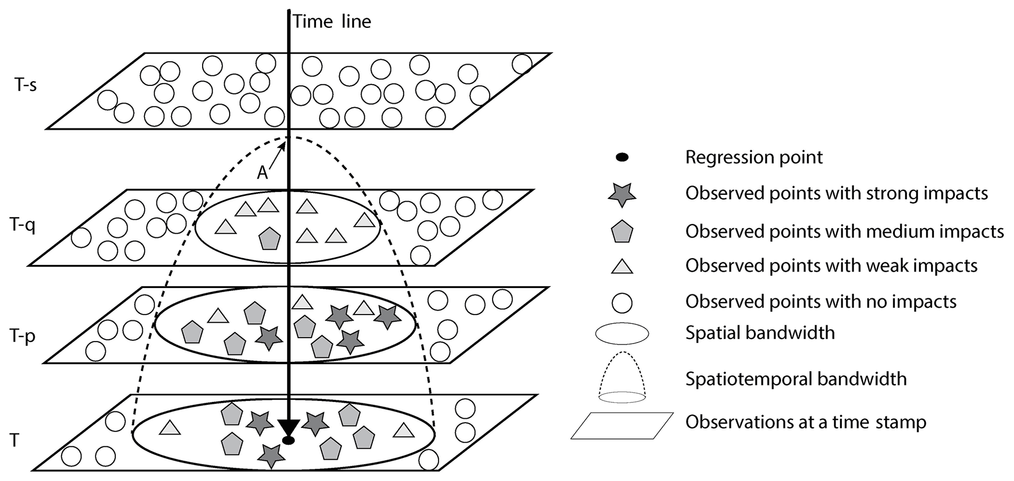
Figure 1 Spatiotemporal impacts of observed points with different rates of value change on a regression point at time stage T. The temporal bandwidth is the length of time from the intersection point A of the spatiotemporal bandwidth and the time line to the regression point. The spatial bandwidth and spatiotemporal bandwidth are illustrated in the figure legend.

GWR has a strategy of spatial distance decay impact on a regression point (Brunsdon et al., 1998; Fotheringham et al., 2003). A similar “time distance decay” strategy was also discussed in several recent GTWR models (Crespo et al., 2007; Huang et al., 2010; Wu et al., 2014; Fotheringham et al., 2015). Yet, those models did not fully reflect the effect of time distance decay. Sample points are observed at different time stages, and those data points closer in time distance to a regression point have more impact on the regression point than those farther away. The time distance refers to the value variation rate between an observed point and a regression point during a certain time interval. For example, in Fig. 1, there are four time stages from old to new: T–s, T–q, T–p, and T. Through a fitting and calibration process, the spatiotemporal bandwidth will be fitted, and the spatiotemporal effects (weights) from observed points to a regression point at time stage T will be calculated by a specific spatiotemporal kernel function. Then, in prediction, the value of a regression point at time stage T can be estimated. Thus, the observed points at time stage T only have a spatial effect on the regression point (Fig. 1). There is a temporal effect from data points at time stages T–p and T–q (shown as stars, pentagons, and triangles in the planes of T–p and T–q in Fig. 1) within a certain spatial bandwidth b_ST at each time stage on the regression point. The time distance decay should reflect the fact that different variations of the observed points have different temporal effects. However, as mentioned in the previous section, many existing GTWR models have applied a strategy of time interval decay instead of time distance decay. Consequently, they regard all the observed points as having the same temporal effect on their neighbor regression point.

Compared to existing GTWR models, the time distance decay strategy of STWR considers the effect of different variations of observed points through time. For example, some data points may have a higher impact on the regression point, though their spatial distance is farther than other points. Figure 1 illustrates the fact that the locations of some star-shaped points are farther away from the regression point than some pentagon-shaped points at time stage T–p, which indicates that there are mixed impacts (spatial impact and temporal impact) on the regression point. The temporal impacts depend on the rate of value variation, which is the value difference between the observed point and the regression point divided by a time interval (e.g., [T–p, T] and [T–q, T–p] are time intervals). If the observed time stage is too long ago or the rate of value variation is too small and exceeds the limit of optimized temporal bandwidth for the regression point (as shown by observations at time stage T–s), the data points at this time stage may have no impact on the regression point. Even though some of those data points may have a huge difference in value and are close to the regression point in space, they are not within the range of the optimized temporal bandwidth. Spatial bandwidths also vary along the time line, and usually the bandwidth gets larger when the observation time is closer to the time stage of the regression point (Fig. 1).

2.2 The spatiotemporal kernel function of STWR

We assume that a set of observed points $O_{\mathrm{\Delta }t}=\mathit{\{}{O}_{N_t}{O}_{N_{t-\mathrm{1}}}{O}_{N_{t-q}}\mathrm{|}\mathrm{\Delta }t=[t-qt\left]\mathit{\right\}}$ is collected during a certain time interval Δt in a study area, where t represents the current time stage and $N_{t-i}i\in \left\{\mathrm{0},\mathrm{1},\mathrm{2},\mathrm{\dots },q\right\}(N_t=N_{t-\mathrm{0}})$ denotes the number of observed points at each recorded time. As in the idea described above, we can borrow neighbor points in space and their value variation during certain recent time intervals, so we can still use Eq. (1) to generate local estimates. The weight matrix W in GWR usually depends on the spatial kernel (Fotheringham et al., 2015). In STWR, we need to consider the temporal effect, so the form of W is different from that in GWR. Correspondingly, we should have a spatiotemporal kernel, which can be understood as a temporal extension based on the spatial kernel. However, if we use a multiplication form to combine the temporal kernel and the spatial kernel (Huang et al., 2010; Wu et al., 2014; Fotheringham et al., 2015), we will face the problem of time and space interaction as mentioned above in the Introduction section. To address that issue, we design a weighted average form for the spatiotemporal kernel.

$$\begin{array}{}\text{(3)}& w_{ij\text{ST}}^t=(\mathrm{1}-\mathit{\alpha })k_{\text{s}}\left(d_{sij}{b}_{\text{ST}}\right)+\mathit{\alpha }{k}_{\text{T}}\left(d_{tij}{b}_{\text{T}}\right),\mathrm{0}\le \mathit{\alpha }\le \mathrm{1}\end{array}$$

In Eq. (3), $w_{ij\text{ST}}^t$ is the weight at time t and at the observed location j. k_s and k_T are the spatial and temporal kernel, respectively, and they both have a value range of 0 to 1. α is an adjustable parameter to scale the temporal and spatial effects, which can be optimized with the bandwidth selections. The role of parameter α is different from the scale parameter τ ($\mathit{\tau }=\frac{u}{\mathit{\lambda }}$) in GTWR (Huang et al., 2010). α is introduced here for adjusting the outputs of the spatial kernel k_s and the temporal kernel k_T, which means measuring the relative strength of the spatial and temporal impacts on the regression point. But the scale parameter τ is used for adjusting the inconsistency of the time distance and space distance, which cannot adjust the relative strength of k_s and k_T. d_sij and d_tij are the spatial (Euclidean) and temporal distance between the regression point i and an observed data point j, respectively. b_ST is the spatial bandwidth b_S at a certain time stage T, and b_T denotes the temporal bandwidth.

The time distance, as mentioned above, is not the time interval but the rate of value variation between an observed point and a regression point through a time interval. Following the time distance decay strategy in STWR, we can further derive the temporal kernel k_T as shown below.

$$\begin{array}{}\text{(4)}& w_{ij\mathrm{\Delta }t}^t=\left\{\begin{array}{l}\left[\frac{\mathrm{2}}{\mathrm{1}+\exp \left(-\frac{\left|(y_{i\left(t\right)}-y_{j(t-q)})/y_{j(t-q)}\right|}{\mathrm{\Delta }t/b_{\text{T}}}\right)}-\mathrm{1}\right]\\ \text{if}\mathrm{0}<\mathrm{\Delta }t<b_{\text{T}}\\ \mathrm{0}\text{otherwise}\end{array}\right.\end{array}$$

In Eq. (4), $y_{i\left(t\right)}-y_{j(t-q)}$ is the subtraction of the regression point i observed value at t from the point j observed value at t–q, which denotes the value change during the time interval Δt. The internal part of the exponential function is negative in order to make the weight $w_{ij\mathrm{\Delta }t}^t$ range from 0 to 1. The faster the value change rate is, the bigger the weight is, which means that the time impact is larger. When the time interval Δt is out of the range (0,b_T), the weight will be set to zero, which indicates that there is no impact because the observed variation is too far to affect the current moment. For example, if the price of a nearby house changed a long time ago, it may have little or no impact on the present house price. But if the house price had a sharp change recently, it will have a big impact on the present house price. Therefore, the faster the rate of observed value change and the shorter the time interval, the greater the impact on the regression point will be. Compared with GTWR models, the advantage of STWR is that the temporal kernel function k_T can better leverage the variation data.

To calibrate the weight value $w_{ij\text{ST}}^t$, we need a spatial kernel function. The most widely used kernel functions are bi-square and Gaussian (Fotheringham et al., 2003), which are given in Eqs. (5) and (6), respectively.

$$\begin{array}{}\text{(5)}& {\displaystyle }& {\displaystyle }\text{Bi-square:}{w}_{ij\text{S}}=\left\{\begin{array}{ll}{\left[\mathrm{1}-{\left(\frac{d_{sij}}{b_{\text{S}}}\right)}^{\mathrm{2}}\right]}^{\mathrm{2}}& \text{if}{d}_{sij}<b_{\text{s}}\\ \mathrm{0},& \text{otherwise}\end{array}\right.\text{(6)}& {\displaystyle }& {\displaystyle }\text{Gaussian:}{w}_{ij\text{S}}=\exp \left[-{\displaystyle \frac{\mathrm{1}}{\mathrm{2}}}{\left({\displaystyle \frac{d_{sij}}{b_{\text{S}}}}\right)}^{\mathrm{2}}\right]\end{array}$$

In Eqs. (5) and (6), b_S is the spatial bandwidth. Derived from b_S and b_ST, b_St is the initial spatial bandwidth at the given time stage t of the regression point (i.e., t is the initial time for searching observed points in the past). Many functions can be specified for the change in spatial bandwidth during the time intervals. Because in most cases it will have a smooth change during a certain short time interval, we assume that the spatial bandwidth changes linearly along with time, as defined below.

$$\begin{array}{}\text{(7)}& b_{\text{ST}}=b_{\text{S}t}-\tan \mathit{\theta }\times \mathrm{\Delta }t,-{\displaystyle \frac{\mathit{\pi }}{\mathrm{2}}}<\mathit{\theta }<{\displaystyle \frac{\mathit{\pi }}{\mathrm{2}}}\end{array}$$

In Eq. (7), tan θ denotes the slope of spatial bandwidth change in correspondence to Δt, and b_St denotes the initial spatial bandwidth at t. Importing Eqs. (4)–(7), the calibration of Eq. (3) can be further derived into Eqs. (8) and (9), which are our spatiotemporal kernel functions in STWR. Equations (8) and (9) are based on the bi-square and Gaussian kernel, respectively. With the STWR spatiotemporal kernel, we only need to optimize the parameters α and θ instead of the spatial bandwidth b_ST. However, we shall traverse all the observed points at the initial time stage t to find the optimized spatial bandwidth b_St. Moreover, we shall also traverse all the time stages to find the optimized temporal bandwidth b_T.

$$\begin{array}{}\text{(8)}& w_{ij\text{ST}}^t=\left\{\begin{array}{l}\left[(\mathrm{1}-\mathit{\alpha })\times {\left[\mathrm{1}-{\left(\frac{d_{sij}}{b_{\text{S}t}-\tan \mathit{\theta }\times \mathrm{\Delta }t}\right)}^{\mathrm{2}}\right]}^{\mathrm{2}}+\mathit{\alpha }\right.\\ \left.\times \left(\mathrm{2}/\left(\mathrm{1}+\exp \left(-\frac{\left|(y_{i\left(t\right)}-y_{j(t-q)})/y_{j(t-q)}\right|}{\mathrm{\Delta }t/b_{\text{T}}}\right)\right)-\mathrm{1}\right)\right]\\ \text{if}\mathrm{\Delta }t<b_{\text{T}},\text{and}{d}_{sij}<(b_{\text{S}t}-\tan \mathit{\theta }\times \mathrm{\Delta }t)\\ \mathrm{0}\text{otherwise}\end{array}\right.\end{array}$$

$$\begin{array}{}\text{(9)}& w_{ij\text{ST}}^t=\left\{\begin{array}{l}\left[(\mathrm{1}-\mathit{\alpha })\times \exp \left[-\frac{\mathrm{1}}{\mathrm{2}}{\left(\frac{d_{sij}}{b_{\text{S}t}-\tan \mathit{\theta }\times \mathrm{\Delta }t}\right)}^{\mathrm{2}}\right]+\mathit{\alpha }\right.\\ \left.\times \left(\mathrm{2}/\left(\mathrm{1}+\exp \left(-\frac{\left|\left(y_{i\left(t\right)}-y_{j(t-q)}\right)/y_{j(t-q)}\right|}{\mathrm{\Delta }t/b_{\text{T}}}\right)\right)-\mathrm{1}\right)\right]\\ \text{if}\mathrm{\Delta }t<b_{\text{T}},\text{and}{d}_{sij}<(b_{\text{S}t}-\tan \mathit{\theta }\times \mathrm{\Delta }t)\\ \mathrm{0}\text{otherwise}\end{array}\right.\end{array}$$

3 STWR in operation

3.1 Bandwidth selection and parameter estimation

Some goodness-of-fit diagnostics (Loader, 1999) are widely used in general GWR-based models, such as the cross-validation (CV) score (Cleveland, 1979; Bowman, 1984) and the Akaike information criterion (AIC) (Akaike, 1973, 1998). For STWR, we use cross-validation (CV) as the default searching criteria and we also calculate the value of a corrected version of AIC (Hurvich et al., 1998), the AICc, which is defined below.

$$\begin{array}{}\text{(10)}& {\text{AIC}}_c=\mathrm{2}n\ln \left(\widehat{\mathit{\sigma }}\right)+n\ln \left(\mathrm{2}\mathit{\pi }\right)+n\left\{{\displaystyle \frac{n+\text{tr}\left(S\right)}{n-\mathrm{2}-\text{tr}\left(S\right)}}\right\}\end{array}$$

In Eq. (10), n is the sample size, $\widehat{\mathit{\sigma }}$ is the estimated standard deviation of the error term, and tr(S) denotes the trace of the hat matrix S (Hoaglin and Welsch, 1978).

Although there is no need to optimize the spatial bandwidth b_ST of the past time stages in STWR, other parameters such as α and θ need to be optimized. Also, we should calculate the b_T and initial b_St through trials. For more potential combinations of these parameters for different spatiotemporal processes, a more reasonable limit and optimization procedure are hence needed.

Figure 2 Weight matrix W_Δt. The symbol $p_k^{(t-i)}i\in \mathrm{0},\mathrm{1},qk\in \mathrm{1},\mathrm{2},N_{t-i}$ denotes the kth observed point at t−i. The symbol $w_{\mathrm{\Delta }t,p_{\text{m}}^{\left(t\right)}{p}_n^{(t-i)}}^{t-i}i\in \mathrm{0},\mathrm{1},qm\in \mathrm{1},\mathrm{2},N_{t}n\in \mathrm{1},\mathrm{2},\mathrm{\dots },N_{t-i}$ denotes the weight of the nth point $p_n^{(t-i)}$ at t−i to the mth point $p_{\text{m}}^{\left(t\right)}$ at t.The symbol $O_{N_{t-i}}i\in \mathrm{0},\mathrm{1},q$ denotes a set of points observed at t−i. Δt denotes all the time intervals of the weight matrix. In the central and right parts of the figure, the records with background shading indicate weight values affected by temporal effects.

3.2 Calibration of STWR

Calibration of STWR models can be conducted by using weighted least squares. The estimator for the coefficients at location (u_iv_i) is shown below.

$$\begin{array}{}\text{(11)}& \begin{array}{rl}& {\widehat{\mathit{\beta }}}_t\left(u_i{v}_i\right)=\\ & \left[{\left({\mathbf{X}}_{O_{\mathrm{\Delta }t}}^T{\mathbf{W}}_{\mathrm{\Delta }t}\left(u_i{v}_i\right){\mathbf{X}}_{O_{\mathrm{\Delta }t}}\right)}^{-\mathrm{1}}{\mathbf{X}}_{O_{\mathrm{\Delta }t}}{\mathbf{W}}_{\mathrm{\Delta }t}\left(u_i{v}_i\right)\right]y_{O_{\mathrm{\Delta }t}}\end{array}\end{array}$$

In Eq. (11), ${\mathbf{X}}_{O_{\mathrm{\Delta }t}}$ and $y_{O_{\mathrm{\Delta }t}}$ are observed independent and dependent variables of O_Δt, respectively. ${\mathbf{X}}_{O_{\mathrm{\Delta }t}}^T$ is the transpose of ${\mathbf{X}}_{O_{\mathrm{\Delta }t}}$. W_Δt(u_iv_i) denotes the spatiotemporal weight matrix for observed points at different locations to the regression point (u_iv_i) at different time stages during Δt. For a better illustration, we show the weight matrix W_Δt during the time interval Δt in Fig. 2. The matrix W_Δt here is a bit different form the W(u_iv_i) in Eq. (2). The records in the ith row of W_Δt are the diagonal elements in W(u_iv_i), and only nonzero values are used to calibrate the coefficients ${\widehat{\mathit{\beta }}}_k$ for each regression point. Thus, each row r of this hat matrix is shown below.

$$\begin{array}{}\text{(12)}& r_{it}=X_{it}{\left({\mathbf{X}}_{\mathrm{\Delta }t}^T{\mathbf{W}}_{i\mathrm{\Delta }t}{\mathbf{X}}_{\mathrm{\Delta }t}\right)}^{-\mathrm{1}}{\mathbf{X}}_{\mathrm{\Delta }t}{\mathbf{W}}_{i\mathrm{\Delta }t}\end{array}$$

In Eq. (12), X_it is the ith row of the matrix of independent variables at t. X_Δt is the matrix of independent variables during a time interval Δt, and ${\mathbf{X}}_{\mathrm{\Delta }t}^T$ is its transpose. Although the X_Δt in Eq. (12) is equal to the ${\mathbf{X}}_{O_{\mathrm{\Delta }t}}$ in Eq. (11) in the fitting and calibration of STWR, we distinguish ${\mathbf{X}}_{O_{\mathrm{\Delta }t}}$ from X_Δt here. Because ${\mathbf{X}}_{O_{\mathrm{\Delta }t}}$ is a specific matrix of independent variables of an observed point set O_Δt during Δt, X_Δt is a general matrix of independent variables of points during Δt. ${\mathbf{X}}_{O_{\mathrm{\Delta }t}}$ is only used for fitting and calibration of STWR, while X_Δt can also be used for prediction in STWR. In other words, we can understand ${\mathbf{X}}_{O_{\mathrm{\Delta }t}}$ as a subclass of X_Δt. W_iΔt is the ith row of the weighted matrix W_Δt.

3.3 Reasonable searching range and procedure of optimization

In order to obtain the optimized α and θ for STWR (Eqs. 8 and 9), the search range should be limited. Here we use the distance from each regression point $p_i^{\left(t\right)}$ to its Mth nearest neighbor as the initial spatial bandwidth b_St at t. The range of b_St is within a finite set of discrete values because the maximum number of nearest neighbors is limited to $N_{t-i}i\in \mathrm{1},\mathrm{2},\mathrm{\dots },q$ for the regression point $p_i^{\left(t\right)}$ (N_t−i is the total number of observed points at t−i). We denote that value set for b_St as $B{S}_{Nt}=\mathit{\{}{D}_{k+\mathrm{1}}{D}_{k+\mathrm{2}}{D}_{N_t}$, in which the element $D_{U}U\in k+\mathrm{1},k+\mathrm{2},\mathrm{\dots },N_t$ denotes the distance from $p_i^{\left(t\right)}$ to the Uth nearest neighbor, and k equals the number of independent variables. Moreover, the searching range of the temporal bandwidth b_T is also limited to a finite discrete set BT_λ={Δt₁Δt₂Δt_λ, in which the element Δt_λ is the time interval from t to t−λ.

The optimization procedure is to traverse the set BT_λ, and for each step we further traverse the set BS_Nt to get the optimized α and θ through trials. Some trials of θ may lead to no solution to Eq. (11) because there might be fewer than (k+1)th neighbors within the radius of b_St−θΔt_λ from the regression point. Therefore, if it occurs at time stage t−λ, the spatial bandwidth b_St−θΔt_λ needs to be extended to the distance from its (k+1)th nearest neighbor to the regression point to guarantee that the matrix in Eq. (11) will be nonsingular.

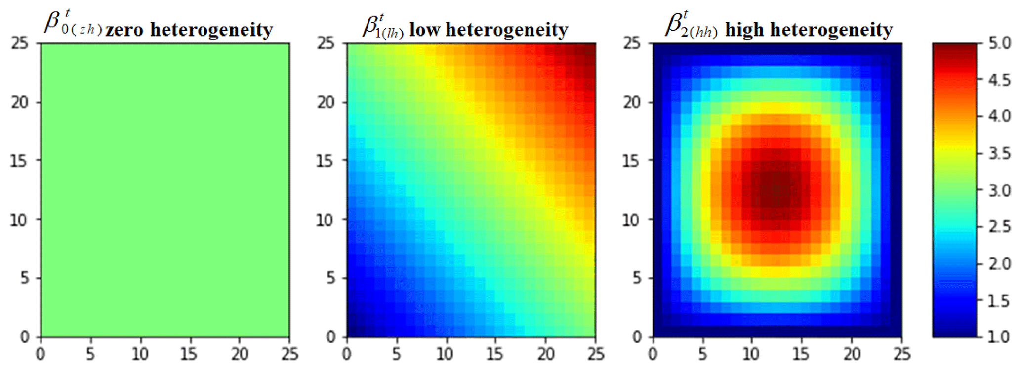
Figure 3 Three simulated initial surfaces for representing the spatial heterogeneity of parameters.

3.4 Steps of using STWR for prediction

In this paper, STWR is used to predict the current values of regression points with known coordinates. The prediction formulas of STWR are more complicated than GWR because the spatial distance is calculated directly from the regression point to each observed data point, while the time distance between the regression point and the data points observed in the past cannot be calculated directly. Therefore, we specify a few steps for prediction in STWR. First, we need to have the optimized initial spatial bandwidth b_St, the optimized α and θ, the optimized number of time stages in the model used, and the fitted weight matrix. Second, all data points within the limited distance of the spatial bandwidth at the latest time stage should be found for the regression point. Third, all the temporal weights of these data points need to be retrieved from the established weight matrix (Fig. 2). Fourth, we use these retrieved weights to calculate (e.g., use mean value or inverse distance weighting value) the temporal weight on the regression point. Fifth, by combining the calculated spatial weight and the optimized α and θ, we can calculate the spatiotemporal weight on the regression point. Then the value of the regression point can be calculated.

4 Experiments with simulated data

4.1 Simulation design

To verify the performance of STWR and compare with the results of GWR and GTWR, several groups of simulated data were used in this study to represent different types of heterogeneity in space and time. All the data and code used in the experiments are shared on GitHub. Web links are provided at the end of this paper.

For GTWR, we only compared with the results generated by algorithms in Huang et al. (2010) and Wu et al. (2014) because we did not find the software package of Fotheringham et al. (2015). The data-generating process (DGP) and the spatial heterogeneity are introduced here. The basic DGP is a linear model shown in Eq. (1), and the study area is a regular 25×25 lattice. We defined three initial surfaces to represent the spatial heterogeneity of parameters (Fig. 3), which were generated by Eqs. (13), (14), and (15) (Fotheringham et al., 2017). Through Eq. (1), the two independent variables x₁ and x₂ were initially generated randomly from the normal distribution $x_{\mathrm{1}}^{\text{initial}}\sim N(\mathrm{100},\mathrm{8})$ and $x_{\mathrm{2}}^{\text{initial}}\sim N(\mathrm{50},\mathrm{6})$, respectively. They can be set as any other values, and the mean values of both distributions may change over time. The error term was generated from a normal distribution $\mathit{\epsilon }\sim N(\mathrm{0},\mathrm{0.5})$.

$$\begin{array}{}\text{(13)}& {\displaystyle }& {\displaystyle }{\mathit{\beta }}_{\mathrm{0}\left(zh\right)}^t=\mathrm{3}\text{(14)}& {\displaystyle }& {\displaystyle }{\mathit{\beta }}_{\mathrm{1}\left(lh\right)}^t=\mathrm{1}+{\displaystyle \frac{\mathrm{1}}{\mathrm{12}}}\left(uv\right)\text{(15)}& {\displaystyle }& {\displaystyle }{\mathit{\beta }}_{\mathrm{2}\left(hh\right)}^t=\mathrm{1}+{\displaystyle \frac{\mathrm{1}}{\mathrm{324}}}\left[\mathrm{36}-{\left(\mathrm{6}-{\displaystyle \frac{u}{\mathrm{2}}}\right)}^{\mathrm{2}}\right]\left[\mathrm{36}-{\left(\mathrm{6}-{\displaystyle \frac{v}{\mathrm{2}}}\right)}^{\mathrm{2}}\right]\end{array}$$

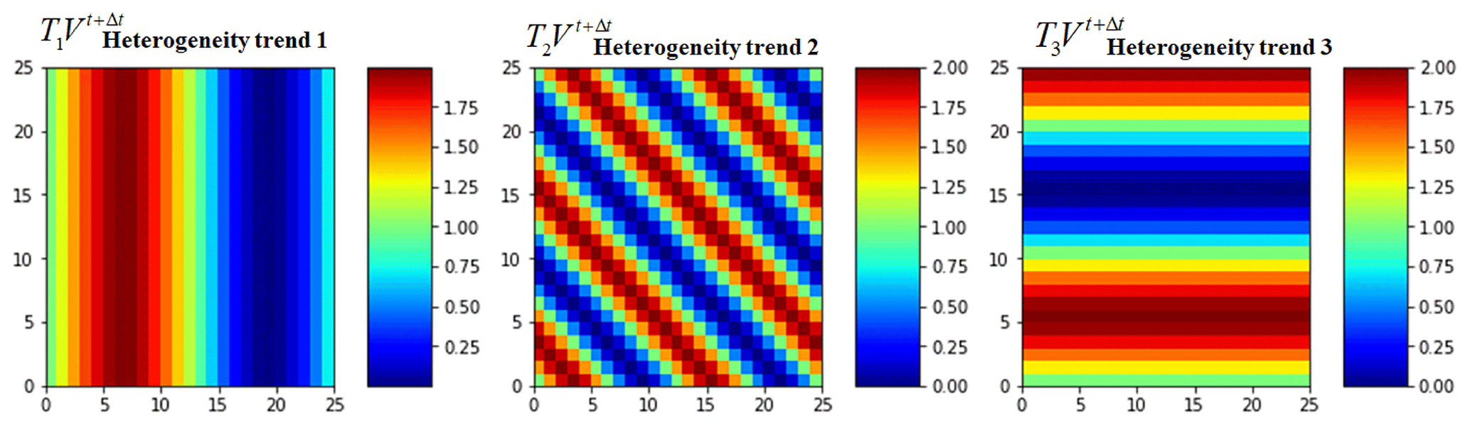
Several trends were designed to simulate the value change. For a better simulation, we assumed that value variation can also be spatial heterogeneity. To distinguish from the heterogeneity of the coefficient surface, three other heterogeneity trend functions were defined by Eqs. (16)–(18).

$$\begin{array}{}\text{(16)}& {\displaystyle }& {\displaystyle }{T}_{\mathrm{1}}{V}^{t+\mathrm{\Delta }t}=V^t+\mathit{\phi }\times \sin (v/\mathrm{4})\mathrm{\Delta }{t}^{n_{\text{power}}}\text{(17)}& {\displaystyle }& {\displaystyle }{T}_{\mathrm{2}}{V}^{t+\mathrm{\Delta }t}=V^t+\mathit{\phi }\times \sin [\mathrm{1}/\mathrm{10}\mathit{\pi }u]\mathrm{\Delta }{t}^{n_{\text{power}}}\text{(18)}& {\displaystyle }& {\displaystyle }{T}_{\mathrm{3}}{V}^{t+\mathrm{\Delta }t}=V^t+\mathit{\phi }\times \sin [\mathrm{1}/\mathrm{6}\mathit{\pi }(u+v\left)\right]\mathrm{\Delta }{t}^{n_{\text{power}}}\end{array}$$

In the above equations, V^t denotes the value at time stage t, φ is used for adjusting the magnitude of change, $\mathrm{\Delta }{t}^{n_{\text{power}}}$ denotes value change with the nth power of the time interval, and $T_i{V}^{t+\mathrm{\Delta }t}i\in \mathrm{1},\mathrm{2},\mathrm{3}\mathit{\}}$ denotes the V value at time stage t+Δt, which is the result of the ith trend function from the V^t. Figure 4 shows these trends when φ, V^t, and $\mathrm{\Delta }{t}^{n_{\text{power}}}$ are set to 1.

Our goal for this experiment was to test model performance by using sample data from the simulation process at different times. Three case studies were designed for different situations. Besides the spatial heterogeneity trends, in our simulation design we assumed that the mean values of two independent variables x₁ and x₂ also changed over time, which were generated by Eqs. (19) and (20), respectively.

$$\begin{array}{}\text{(19)}& {\displaystyle }& {\displaystyle }{T}_{\mathrm{1}}{x}_{\text{m}}^{t+\mathrm{\Delta }t}=x_{\text{m}}^t\pm {\mathit{\eta }}_{\mathrm{1}}\times \mathrm{\Delta }t\text{(20)}& {\displaystyle }& {\displaystyle }{T}_{\mathrm{2}}{x}_{\text{m}}^{t+\mathrm{\Delta }t}=x_{\text{m}}^t\pm {\mathit{\eta }}_{\mathrm{2}}\times \mathrm{\Delta }t\end{array}$$

In the above two equations, $x_{\text{m}}^t$ denotes the mean of an independent variable x at time stage t, $T_i{x}_{\text{m}}^{t+\mathrm{\Delta }t}i\in \mathrm{1},\mathrm{2}\mathit{\}}$ denotes the mean of x at time stage t+Δt, and η₁ and η₂ are two parameters for adjusting the rate of change. At each time stage during the simulations, the independent variables x₁ and x₂ are generated by a normal distribution with new means of $T_{\mathrm{1}}{x}_{\text{m}}^{t+\mathrm{\Delta }t}$ and $T_{\mathrm{2}}{x}_{\text{m}}^{t+\mathrm{\Delta }t}$, respectively.

Figure 4 Three heterogeneity trend surfaces.

4.2 Results with simulated data

We compared the results of OLS, GWR, GTWR, and STWR. A total of 333 random sample points for five time stages (t₀, t₁, t₂, t₃, and t₄ from old to new) were collected from the 25×25 lattice generated in the abovementioned DGP. To simplify the calculation process, we set θ in Eq. (7) to zero. Due to the limitation of paper length, in the comparison below the STWR results only include those generated by the spatiotemporal kernel in Eq. (8). The objective is to compare the predicted results with the true value at the latest time stage.

Table 1 Results of case study 1 at time stage t₄.

4.2.1 Case study 1

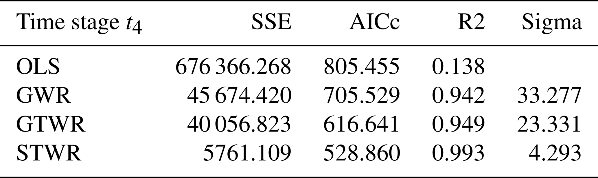
The time interval of observations in case study 1 was one unit, such as 1 s or 1 d. The value changes of x₁ and x₂ were generated by η₁=0.5 and η₂=0.1 and were affected by T₁V with φ=0.5 and n_power=1. This means that x₁ and x₂ only changed slightly over time. Table 1 presents the results of the global OLS, GWR, GTWR, and STWR at the latest time stage, i.e., stage 5. It shows that the sum of squared errors (SSEs) of prediction in STWR is much lower than the other models by at least 1 order of magnitude. In addition, the AICc scores (Eq. 10) also show that STWR outperforms GTWR and GWR. As shown in Table 1, the R² (average R-squared value of all regression points) value increases from 13.8 % in OLS to 94.2 % in GWR, 94.9 % in GTWR, and 99.3 % in STWR. The estimated standard error, sigma, is reduced to 4.292 in STWR from 23.331 in GTWR. Also, Fig. 5 shows that both the prediction surface (Y_pred) and the prediction error surface (Pred_Error) of STWR are more accurate than those in GWR. Due to the limitation of the software package in Huang et al. (2010) and Wu et al. (2014), we did not generate images for GTWR in Fig. 5, but the result can be seen from the sigma value in Table 1.

Table 2 Results of case study 2 at time stage t₄.

4.2.2 Case study 2

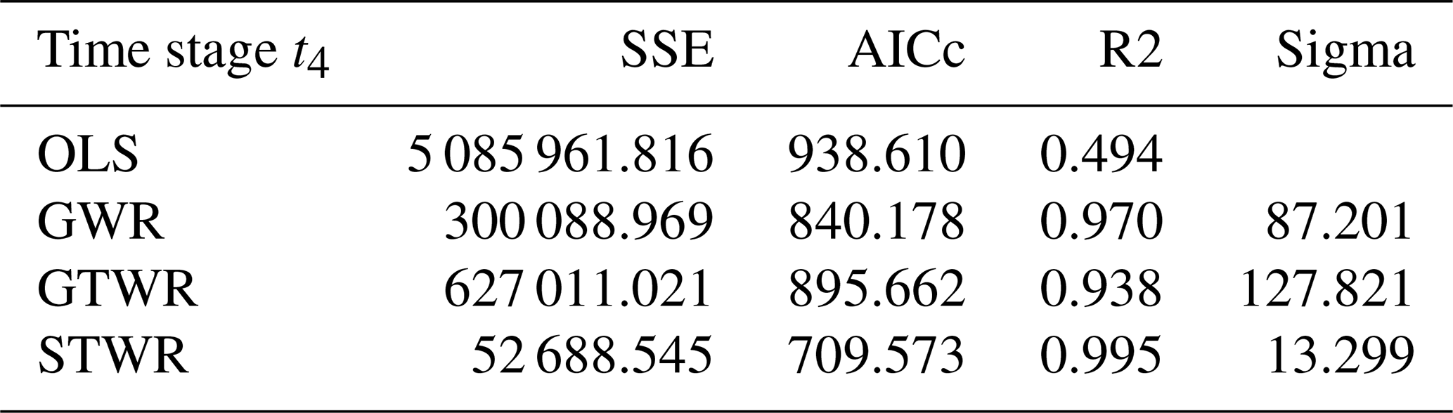
The time interval of observations in case study 2 was 10 units. The value change of x₁ was generated by η₁=0.5 and affected by T₃V with φ=0.5, and n_power=2. x₂ was generated by η₂=2 and affected by T₂V with φ=1 and n_power=1, which indicates that x₁ and x₂ changed fast over time. Table 2 shows the results of the global OLS, GWR, GTWR, and STWR at time stage 5. The SSE value in STWR is much lower than other models, and STWR has the highest R² value of 0.995. The sigma value of STWR is 13.299, which is the lowest and less than one-fifth of the sigma in GWR and less than one-sixth of the sigma in GTWR. The AICc scores also show that STWR significantly outperforms GTWR and GWR.

STWR utilized data from the latest three time stages to calibrate the model. The initial spatial bandwidth b_St of STWR was three nearest neighbors, which was smaller than the one in GWR with 15 nearest neighbors. The optimized α of STWR was 0.08, which shows that the effect of the observed points used on their local regression points was mainly determined by their spatial distance. In this case, the GWR outperforms GTWR, which may due to the higher ratio of value change. Compared with the y_true surface, the prediction surface of STWR is much better than GWR (Fig. 6). For the same reason as mentioned in case study 1, we did not generate images for GTWR in Fig. 6.

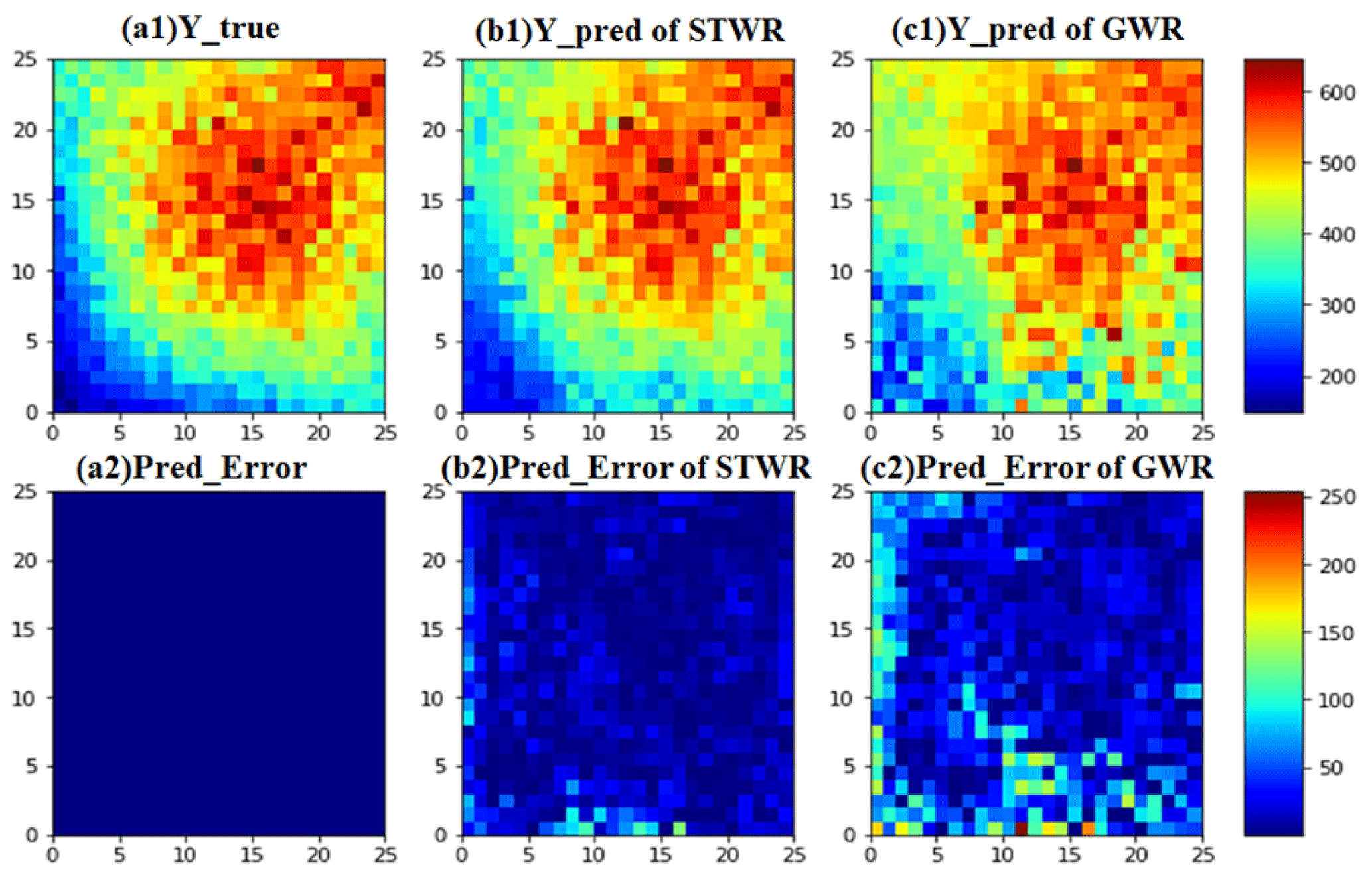
Figure 5 Comparing prediction results of STWR and GWR in case study 1. Images (a1), (b1), and (c1) are the simulation surfaces of true Y, the predicted surface of Y by STWR, and the predicted surface of Y by GWR, respectively. Images (a2), (b2), and (c2) are the surface of simulation error, the surface of prediction error of STWR, and the surface of prediction error of GWR, respectively.

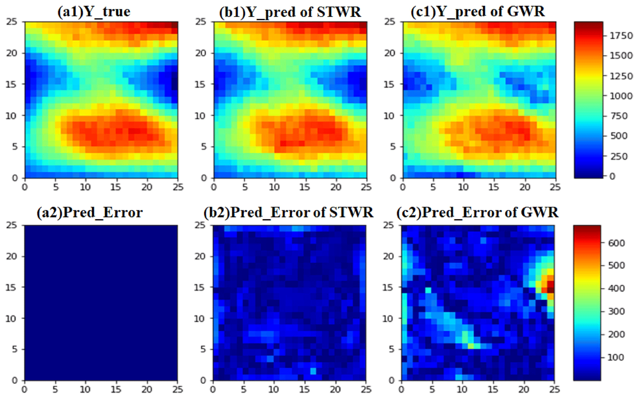
Figure 6 Comparing prediction results of STWR and GWR in case study 2. Images (a1), (b1), and (c1) are the simulation surfaces of true Y, predicted surface of Y by STWR, and predicted surface of Y by GWR, respectively. Images (a2), (b2), and (c2) are the surface of simulation error, the surface of prediction error of STWR, and the surface of prediction error of GWR, respectively.

4.2.3 Case study 3

The time interval of observations in case study 3 was 200 units. In both case studies 1 and 2, the coefficients in Eq. (1) were unchanged. In contrast, in case study 3, three surfaces of coefficients changed over time, which were generated by the trends T₁V, T₂V, and T₃V. The variations of coefficients were assumed to be slow. The φ and n_power in each trend were set to be 0.2 and 1, respectively. Both η₁ and η₂ were set to be 0.5. The dynamic process of the three surfaces of coefficients and the y_true surface at each time stage are shown in Fig. 7. The process in case study 3 is more complicated than a general process, but it may be closer to reality.

Figure 7 Dynamic process of three surfaces of coefficients and the y_true surface at five different time stages.

Results of these comparisons in case study 3 show that STWR outperforms both GWR and GTWR in the accuracy of the model and the effectiveness of the simulation process (Fig. 8a). Along with the change in the coefficients and the increase in x₁ and x₂, the R² values of both GWR and GTWR are consistent in the five time stages, showing an overall downward trend. But the R² of STWR is stable and at a high level among the five time stages. At the beginning stage t₀, the R² values of the three models are similar because there are no previous observations that can be used by STWR and GTWR. The small difference among these models at t₀ may be caused by their different searching range of spatial bandwidth. Starting from time stage t₁, STWR and GTWR can borrow points from previous observations. At time stage t₁, STWR outperforms both GWR and GTWR, and the advantage of STWR becomes more obvious in the later stages.

It may seem strange that GWR can outperform GTWR (Fig. 8), but that is reasonable for the process in case study 3. The change in this process is faster, and the time interval of observations is bigger than the previous case studies. STWR is not only able to deal with time intervals, but also to make full use of the value variation of observed points for calibration. In contrast, GTWR only uses the time interval information and all the observed points to calibrate, which may cause problems when the observed values are significantly different in spatial distribution or the time intervals are long. GTWR makes use of points from previous time stages without considering their variation, but if the actual values are quite different from previous observations at the current time stage, all the point values for the calibration of GTWR will become smooth. Thus, GWR outperforms GTWR in this situation because GWR only uses the current data points for model calibration.

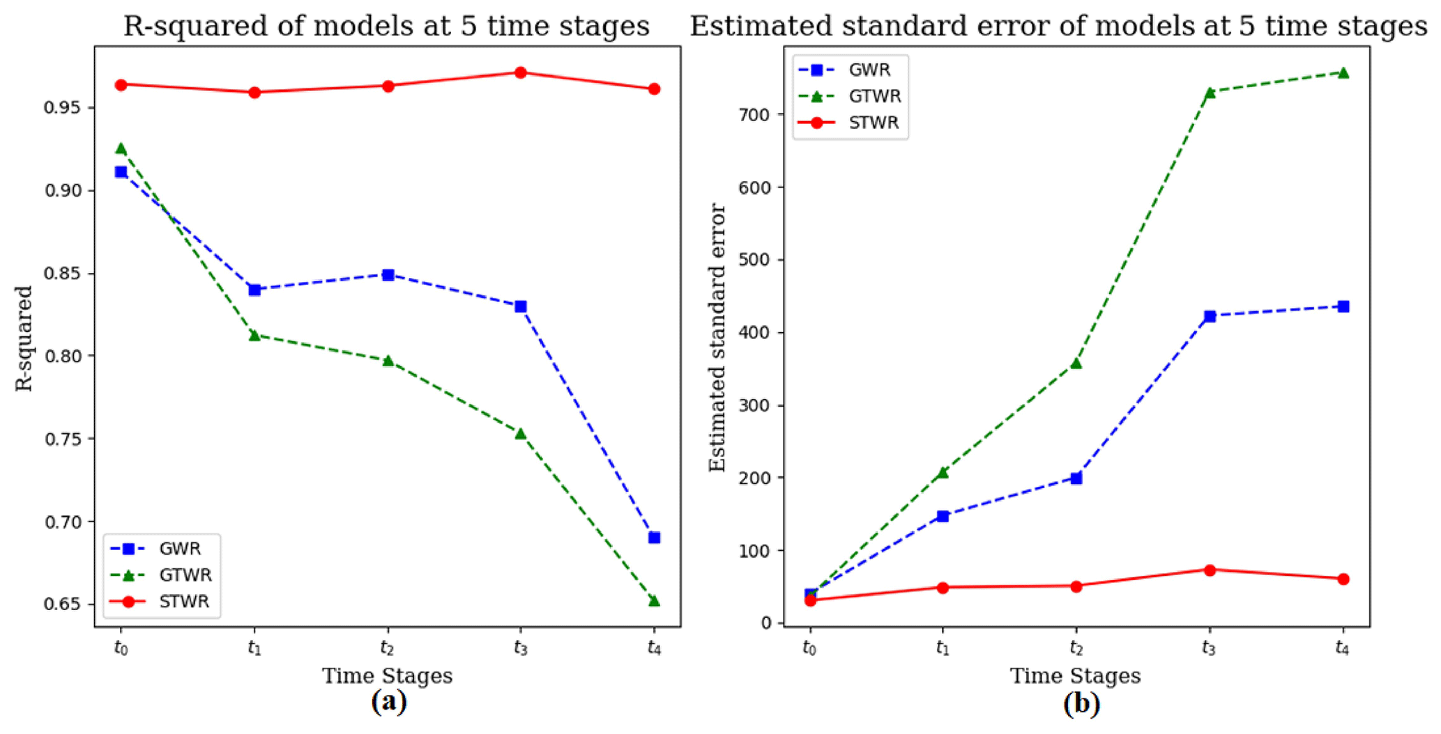
Figure 8 Comparing and evaluating the performance of GWR, GTWR, and STWR at five time stages. (a) Comparing the R² value of different models; (b) comparing the sigma value of different models.

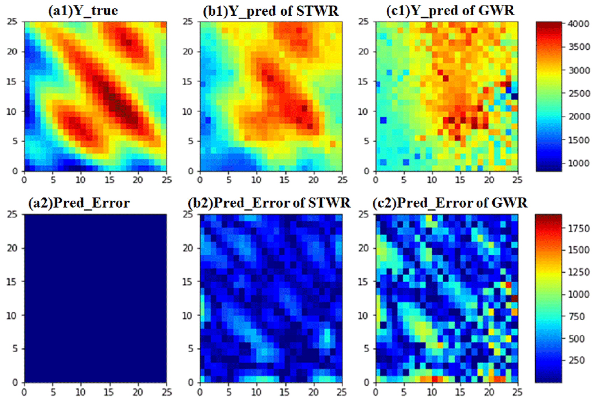
Figure 9 Comparing prediction results of STWR and GWR in case study 3. Images (a1), (b1), and (c1) are the simulation surfaces of true Y, the predicted surface of Y by STWR, and the predicted surface of Y by GWR, respectively. Images (a2), (b2), (c2) are the surface of simulation error, the surface of prediction error of STWR, and the surface of prediction error of GWR, respectively.

STWR is better for estimation than GWR and GTWR because its sigma value is much smaller. As shown in Fig. 8b, the sigma of STWR was half of GWR at time stage t₁ and less than a third of GWR at time stage t₄. The results show that the advantage of STWR is obvious compared with GWR and GTWR.

At t₄, STWR used data from all the past time stages to calibrate the model, and its optimized (initial) spatial bandwidth b_St was derived from four nearest neighbors, which was smaller than the one in GWR with 25 nearest neighbors. The optimized α of STWR was 0, which means that STWR only borrowed points from past time stages without considering their temporal weights on each regression point at t₄. The prediction surfaces at time stage t₄ are shown in Fig. 9. The Y_pred surface of STWR is much better than GWR, especially in the middle and bottom left parts of the surface. The Pred_Error of STWR is also much lower than GWR at almost every location. In this case, the α of STWR at each time stage was 0, 0.96, 0, 0.07, and 0. These values indicate that the temporal effects are different at each stage. They also show that the value of α can be adaptive to scale the temporal and spatial effects (see Eq. 3).

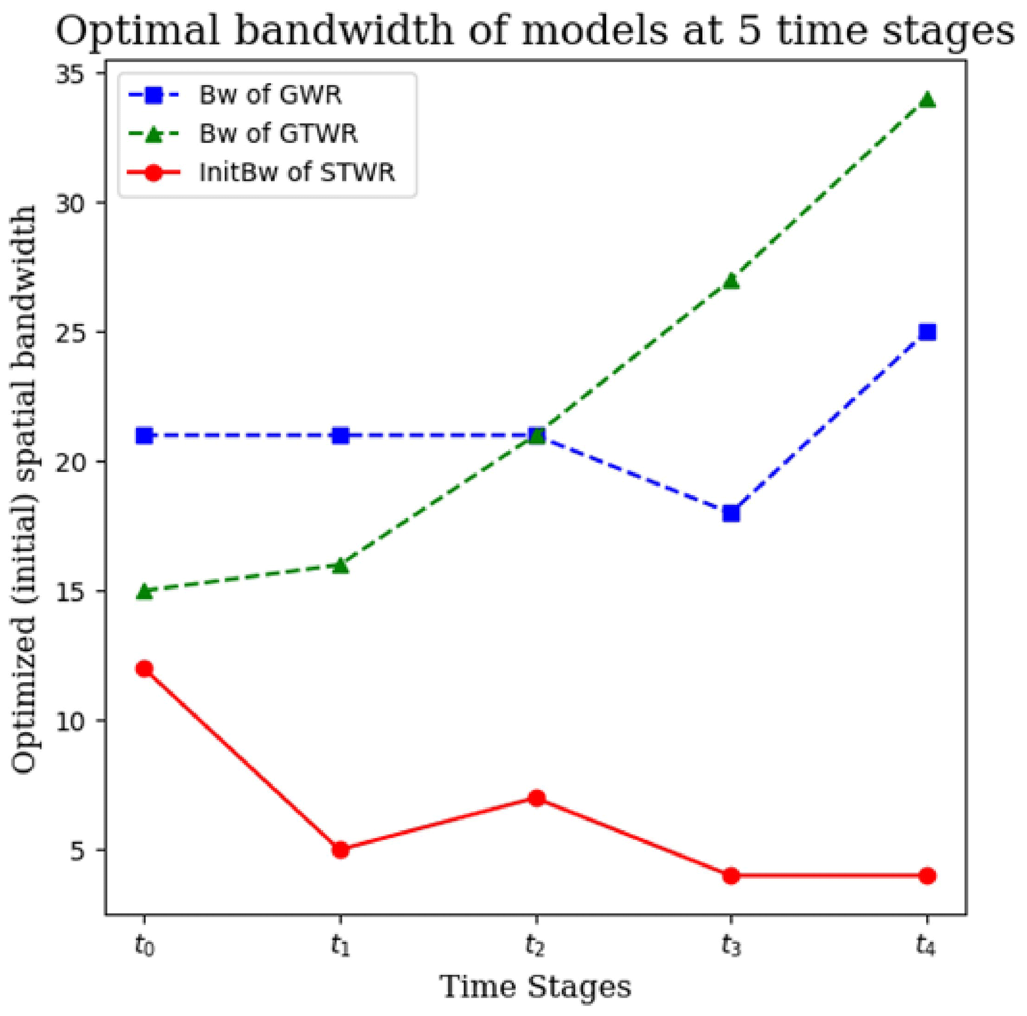
Figure 10 Optimized bandwidths (or initial bandwidths) of GWR, GTWR, and STWR for the five time stages in case study 3.

As Fig. 10 shows, the optimized bandwidths are quite different among these models, and the bandwidths of GWR and GTWR are larger than the initial bandwidth of STWR at each time stage. The optimized bandwidth for each time stage refers to an optimized number of the nearest neighbors (see Sect. 3.3). As GTWR considers all the nearest neighbors from different time stages, the optimized numbers of the nearest neighbors (bandwidth) grow fast and exceed the GWR model at time stage t₂. However, the actual distance from the observed points to the regression points is not necessarily farther. The initial optimized numbers of the nearest neighbors of STWR are smaller than those in GWR and GTWR, which means that the initial spatial bandwidth is narrower than the bandwidth of GWR and GTWR. Nevertheless, due to the strategy of borrowing points from nearby neighbors of past observations, the total points for model calibration in STWR may still be more than GWR and GTWR. Therefore, the initial optimized numbers of the nearest neighbors in STWR are kept at a lower level, which means it is more localized than GWR in this sense.

5 Experiments with real-world data

To further test the performance of STWR, we used data on precipitation δ²H isotopes in the northeastern United States in another case study. We chose δ²H data in 3 d from 29 to 31 October 2012, which includes enough spatiotemporal data for the test. Here in the comparison the STWR results only include those generated by the spatiotemporal kernel in Eq. (8). The data and code used here are shared on Zenodo (see DOI and web links in the “Code and data availability” section at the end of the main text of this article).

In the experiments, we collected a total of 782 measurements from 116 sites located in the northeastern United States during the 3 d period and prepared the data on a daily average. The daily precipitation, mean temperature, and elevation were used as explanatory variables. The model derived from Eq. (1) is represented below.

$$\begin{array}{}\text{(21)}& y_i={\mathit{\beta }}_{\mathrm{0}}+{\mathit{\beta }}_{\mathrm{1}}\text{ppt}+{\mathit{\beta }}_{\mathrm{2}}{t}_{\text{mean}}+{\mathit{\beta }}_{\mathrm{3}}\text{height}+{\mathit{\epsilon }}_i\end{array}$$

In Eq. (21), “ppt” denotes the daily total precipitation (rain + melted snow), t_mean denotes daily mean temperature, and “height” is the elevation value. After data preprocessing, there were 272 points for model calibration and 73 point values on 31 October 2012. For the first day, both GTWR and STWR took no information from the past. Therefore, we only show the results of SSE, R², and the optimized initial neighbor (bandwidth) in the model comparisons for the second and third day (D2 and D3) in Tables 3. The SSE of STWR is the lowest on both days. GWR shows a slightly higher SSE than GTWR at D2 and D3. The R² of STWR is the highest on both days among these models. GWR has a lower R² than GTWR at D2 and almost the same R² as GTWR at D3.

Similar to the experiments on three simulation datasets, the result here shows that STWR outperforms GTWR and GWR. In the experiment, the number of optimized initial neighbors of STWR was smaller than that of GWR and GTWR. The optimized α of STWR was 0 at both D2 and D3. The optimized temporal bandwidths of STWR (number of time stages in the model used) in both D2 and D3 were 2, which means that the STWR in this case only borrowed data points from the latest two time stages for D2 and D3. In the result (Table 3), an interesting point is that the numbers of optimized initial neighbors of STWR are smaller than the spatial bandwidths of GWR for D2 and D3. The reason is that STWR borrowed points from past time stages in the calculation, which led to narrower bandwidths to some extent.

Table 3 Results of model performance with real-world data.

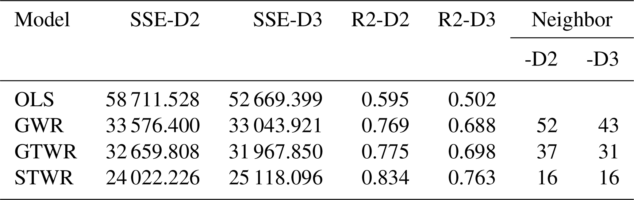
Figure 11 LOOCV results of STWR and GWR. (a) Squared error of prediction at each point (leave out); (b) box plot of the LOOCV results of GWR and STWR.

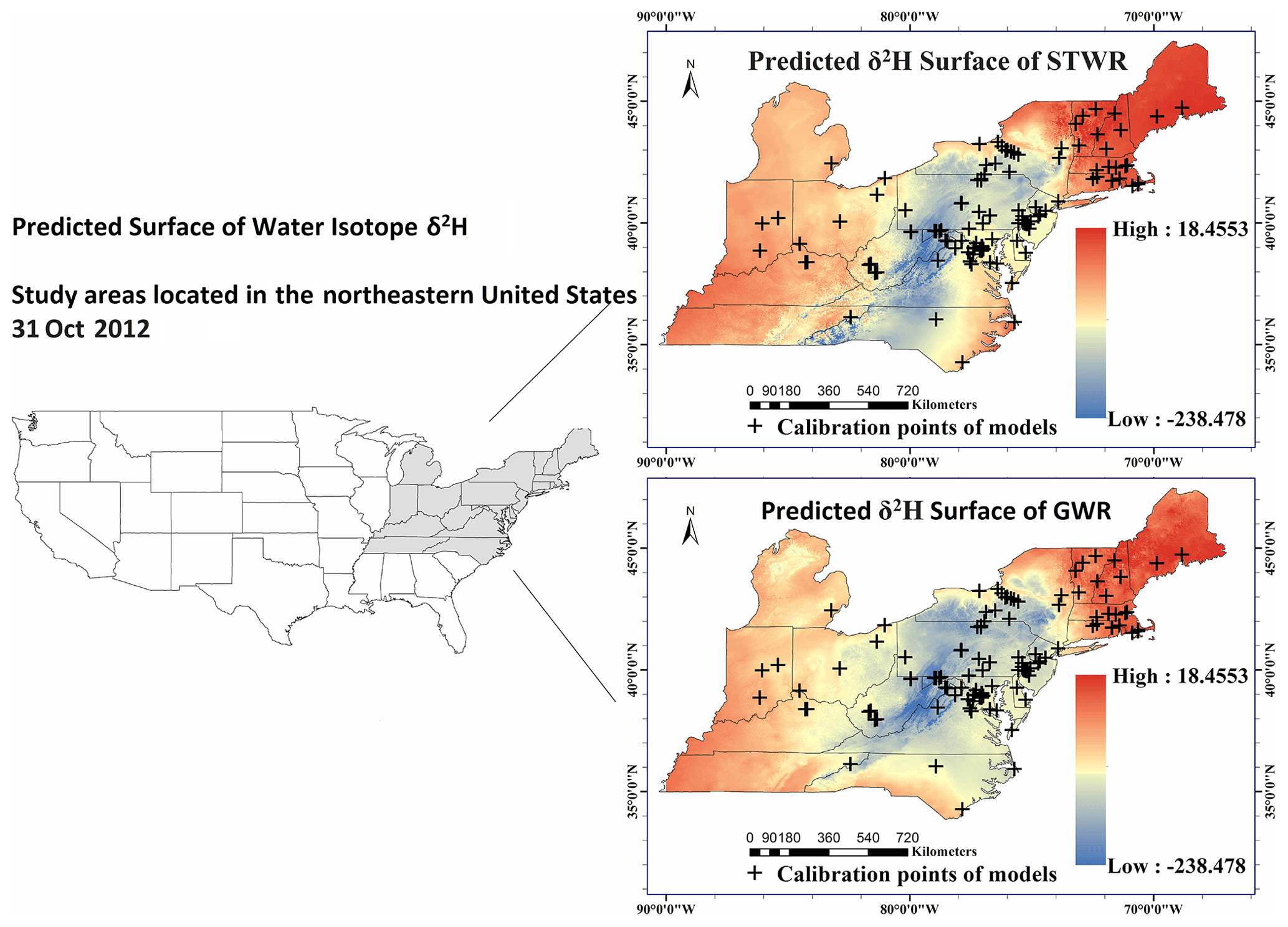
Figure 12 Predicted δ²H surfaces of STWR and GWR at D3.

We adopted leave-one-out cross-validation (LOOCV) at D3 for the comparison between STWR and GWR. The squared errors (SEs) of prediction are shown in Fig. 11. The prediction results of STWR are better than GWR for most points. The mean SE of STWR is smaller than GWR. Moreover, the SE of STWR shows a narrower regional trend, which indicates that STWR is more robust than GWR. In addition, the total SSEs of GWR and STWR are 50 216.510 and 39 724.995, respectively. Therefore, the result further validates the fact that the quality of predication in STWR is better than GWR.

In Fig. 12, the predicted δ²H surface at D3 is broadly similar between the GWR and STWR calibrations. The percentages of explanation of variance in GWR and STWR are similar, which are 68.8 % and 76.3 %, respectively. However, like the experiment results with simulated data (Fig. 10), STWR has a narrower initial bandwidth, which generates more localization in the predicted δ²H surface than GWR. For instance, the lower (light yellow and blue parts) and higher (orange parts) predicted values of δ²H are more concentrated in the δ²H surface of STWR than that of GWR (Fig. 12).

6 Discussion and conclusions

Spatiotemporal data analysis is important in many scientific studies. Due to the complexity of spatiotemporal models, the spatiotemporal effect may not be fully taken into account when the temporal and spatial information is manipulated simultaneously. In particular, models for the effect of spatial dynamics should not be simply adapted for modeling the effect of temporal dynamics. Although the GTWR model can borrow points from the recent past, without careful consideration of the temporal effect, the performance of GTWR may be even worse than GWR. Increasingly, many scientific issues are not just about spatial nonstationary but involve many spatiotemporal processes. It is necessary to review the limitations of current spatiotemporal models and make new extensions. The aim of the STWR model developed in this study is to advance work and discussion in that direction.

Based on a concept similar to GWR, a recently proposed model, called geographically neural network weighted regression (GNNWR) (Du et al., 2020), utilizes both OLS and neural networks to evaluate spatial nonstationarity. It is characterized by a designed spatially weighted neural network (SWNN) that can represent the spatial nonstationary weight matrix in spatial processes. Additionally, a geographically and temporally neural network weighted regression (GTNNWR) model (Wu et al., 2020), which is a temporal extension of GNNWR, was also proposed by the same group for further modeling spatiotemporal nonstationary relationships. GTNNWR can generate a space–time distance by utilizing the so-called spatiotemporal proximity neural network (STPNN), which may address complex nonlinear interactions between time and space. Although both STWR and GTNNWR have the potential to handle complex spatiotemporal nonstationarity in various natural and socioeconomic processes, their principles and interpretability are different.

1. The basic formulation of GNNWR is defined as Eq. (22) (Du et al., 2020), which is different from Eq. (1) (Fotheringham et al., 2003). The w₀(u_iv_i) and w_k(u_iv_i) denote the geographical weight of the constant coefficient β₀ and coefficient β_k, respectively. It is assumed that the multiplication of w_p(u_iv_i) and β_p is equal to β_p(u_iv_i) ($\mathrm{0}\le p\le k)$. The combined β_p(u_iv_i) is thought of as the same as the coefficients of GWR. But in STWR and GWR, the weights and the estimated coefficients are separated. The weights mainly reflect the degree of influence from the observed points on the regression point, while the coefficient values reflect the relationships between the independent variable and dependent variable.

   $$\begin{array}{}\text{(22)}& \begin{array}{rl}& y_i=w_{\mathrm{0}}\left(u_i{v}_i\right){\mathit{\beta }}_{\mathrm{0}}+\sum _{k=\mathrm{1}}^p{w}_k(u_i,v_i){\mathit{\beta }}_k{x}_{ik}+{\mathit{\epsilon }}_i,\\ & i=\mathrm{1},\mathrm{2},\mathrm{\dots },n\end{array}\end{array}$$

2. GTNNWR and GNNWR use the proposed ANN-based method (Eq. 23) (Du et al., 2020) to calculate the weighted matrix, which is quite different from the kernel functions used in GWR and STWR models. Although GTNNWR and GNNWR use the idea of pointwise regression, they do not consider how to “borrow points” from nearby neighbors and do not have the concept of bandwidth. Without a spatial bandwidth, all observation points in the study area may have impacts on the regression point, which might violate Tobler's first law of geography (Tobler, 1970). It may be difficult to understand the relationships between the influence weight and the spatial distances, especially when the study area and the data amounts are large. STWR has spatial bandwidths and follows Tobler's first law of geography, which can help analyze the affected range of local regression points.

   $$\begin{array}{}\text{(23)}& {\mathbf{W}}_i=\mathbf{W}\left(u_i{v}_i\right)=\text{SWNN}\left({\left[d_{i\mathrm{1}}^s,d_{i\mathrm{2}}^s,\mathrm{\dots },d_{in}^s\right]}^T\right)\end{array}$$

3. The data points will be divided into a training set (including a validation set) and test set for GTNNWR and GNNWR, which might require more data points. Thus, it may not be appropriate for analyzing fewer data points (data acquisition in many geoscience processes is difficult and costly). STWR and GWR do not need to divide data points into the training set (including a validation set) and test set, which requires fewer data points than GNNWR and GTNNWR.

4. Although GTNNWR utilizes a method called spatiotemporal proximity neural network (STPNN) (Wu et al., 2020) to calculate the spatiotemporal distance, the obtained integrated spatiotemporal distance lacks explanation, and it is also impossible to tell which parts of the calculated weight are affected by time or space. There is also no concept of a temporal bandwidth in GTNNWR. Therefore, it fails to provide information on the earliest time (stage) at which the observed points start to exert an impact on the determination of the regression point. But STWR has a temporal bandwidth, and it can distinguish the strength of temporal weight and spatial weight. Therefore, we can analyze the characteristics of the local interaction of time and space according to the temporal bandwidth, spatial bandwidth, and the adjustment parameter α.

The temporal kernel and the spatiotemporal kernel functions are two important contributions of STWR. The temporal kernel in STWR applies an improved sigmoid form (see Eq. 4), which is different from the methods for temporal effect analysis in previous GTWR models. The temporal weight generated by the STWR temporal kernel is limited to a value between 0 and 1. The spatial weight in STWR is also limited to a value between 0 and 1. The STWR spatiotemporal kernel function has a weight adjustment parameter α to scale the temporal and spatial weights (Eq. 3). In practice, α can be obtained through optimization. This form of weighted average between temporal and spatial effects in the STWR spatiotemporal kernel is a big improvement compared with the multiplication form in previous GTWR models. The advantage of the STWR spatiotemporal kernel has been proven in four case studies with both simulated and real-world datasets.

Though the performance of STWR is outstanding, the models can still be further extended. A big topic is the time distance. In current STWR, the time distance represents the rate of value variation between an observed point and a regression point through a time interval. Nevertheless, we can also use time distance to represent the rate of value variation at each observed point object through time. Note that, from an object-oriented perspective, here we differentiate the point objects from locations, although the point objects have geospatial coordinates as part of their attributes. Following that new definition of time distance, the $y_{i\left(t\right)}-y_{j(t-q)}$ in the STWR temporal kernel (Eq. 4) can be replaced by Δy_j(t−q) (value variation of an observed point object during Δt). A scenario of interest is that the observed point objects in the past time stages (such as those shown in Fig. 1) may move to new locations, have no value for a few time stages, or even disappear, so the Δy_j(t−q) may not exist. We can use object-based methods to address issues caused by that scenario. For example, each point object can be assigned a unique ID, and then the observed value of the point object at each time stage can be retrieved by using its ID. With this new definition of time distance, the temporal weight on a regression point object is determined by the rate of value variation of its nearby point objects. Several different scenarios for a regression point object at current time stage t are discussed here.

1. The location of an observed point object j is fixed through time (e.g., a fixed sensor). If the value of j is observed at both time stages t and t–q, then Δy_j(t−q) can be calculated directly. If the value of j is observed at t but not observed at t–q, we can use interpolation to generate a value for j at t–q. If the value of j is not observed at t, but the variation in the past is observed, we can use prediction methods to generate a value for j at t.

2. The location of j is not fixed through time (i.e., j moves). If the moving point objects can still have temporal effects on the regression point, then the Δy_j(t−q) can be calculated. The spatial effect, however, depends on whether j moves out of the spatial bandwidth from the regression point or not.

3. j disappears or appears at a certain time stage. If j does not appear until the current time stage t, the Δy_j(t−q) can be set to be 0. If j appears in a past time stage (e.g., t−q) but it disappears before or at t, we can ignore the impact of j for the regression point object.

There are other possibilities for the further improvement of STWR. The first involves the optimization of θ in the spatiotemporal kernel (Eqs. 8 and 9). The slope θ indicates that the variation of the spatial bandwidth is in a linear form, but it may not be a perfect solution. In many situations, the change in the spatial bandwidth over time may not be linear. The second involves making predications for future time stages. In this paper, we only predict values for points at the current time stage t. Extensions can be made in STWR to predict values for points in future time stages beyond t. The third involves exploring multiple spatial and temporal bandwidths of models. Different variables may have different spatial and temporal bandwidths due to their unique characteristics. Correspondingly, we may need more bandwidths to capture the different nonstationarities of those independent variables to better represent the spatiotemporal heterogeneity.

In short, the core contribution of STWR is the clarification of the “time distance” concept and the new temporal kernel and spatiotemporal kernel functions based on this concept. Our experiments show that STWR outperforms GWR and GTWR in analyzing and interpreting local spatiotemporal nonstationarity. We hope STWR can bring fresh ideas and new capabilities for spatiotemporal data analysis in many disciplines.