Numerical integrators for Lagrangian oceanography

A common task in Lagrangian oceanography is to calculate a large number of drifter trajectories from a velocity field precalculated with an ocean model. Mathematically, this is simply numerical integration of an ordinary differential equation (ODE), for which a wide range of different methods exist. However, the discrete nature of the modelled ocean currents requires interpolation of the velocity field in both space and time, and the choice of interpolation scheme has implications for the accuracy and efficiency of the different numerical ODE methods.

We investigate trajectory calculation in modelled ocean currents with 800 m, 4 km, and 20 km horizontal resolution, in combination with linear, cubic and quintic spline interpolation. We use fixed-step Runge–Kutta integrators of orders 1–4, as well as three variable-step Runge–Kutta methods (Bogacki–Shampine 3(2), Dormand–Prince 5(4) and 8(7)). Additionally, we design and test modified special-purpose variants of the three variable-step integrators, which are better able to handle discontinuous derivatives in an interpolated velocity field.

Our results show that the optimal choice of ODE integrator depends on the resolution of the ocean model, the degree of interpolation, and the desired accuracy. For cubic interpolation, the commonly used Dormand–Prince 5(4) is rarely the most efficient choice. We find that in many cases, our special-purpose integrators can improve accuracy by many orders of magnitude over their standard counterparts, with no increase in computational effort. Equivalently, the special-purpose integrators can provide the same accuracy as standard methods at a reduced computational cost. The best results are seen for coarser resolutions (4 and 20 km), thus the special-purpose integrators are particularly advantageous for research using regional to global ocean models to compute large numbers of trajectories. Our results are also applicable to trajectory computations on data from atmospheric models.

1 Introduction

Calculating trajectories of tracers through a precalculated velocity field is a common task for many applications (van Sebille et al., 2018). Oceanic and atmospheric transport simulations are frequently built on this approach, and used to calculate, for example, the transport of pollutants (see, e.g. Rye et al., 1998; North et al., 2011; Povinec et al., 2013; Onink et al., 2019), distribution of algae and plankton (see, e.g. Siegel et al., 2003; Woods, 2005; Visser, 2008), search and rescue operations (see, e.g. Breivik and Allen, 2008; Serra et al., 2020), or temperature and salinity pathways (see, e.g. Barkan et al., 2017). Similarly, climate change studies may compute vast numbers of trajectories to understand transport of heat and salt (see, e.g. Dugstad et al., 2019). Computation of trajectories for a variety of atmospheric species is also a common application (see, e.g. Sirois and Bottenheim, 1995; Riuttanen et al., 2013; Nieto and Gimeno, 2019). Other applications include the calculation of Lagrangian Coherent Structures (LCSs), which is not a transport simulation per se, but which still uses tracer trajectories to analyse flow fields (see, e.g. Farazmand and Haller, 2012; Onu et al., 2015; Haller, 2015; Duran et al., 2018).

For all these applications, it is of interest to obtain trajectories of the desired accuracy with minimal computational work or conversely to obtain the most accurate solution possible for a given amount of computational effort. Marine and atmospheric transport applications often require computing large numbers of trajectories, which are essentially solutions of an ordinary differential equation (ODE). As this can be computationally quite demanding, guidance on how to select the optimal combination of numerical schemes for a given application is of practical value.

We further note that in ODE parlance, the velocity fields represented by ocean currents (and wind) may be both stable and unstable, often presenting hyperbolic points where initially small errors may grow exponentially. It may therefore be useful to employ higher-order integration methods or small time steps with lower-order integration methods. This is particularly relevant for long integration times (months to years) where errors accumulate and can be amplified.

In the applied mathematics community, a standard first choice for numerically solving an ODE is a variable-step integrator (see, e.g. Gladwell et al., 2003). Variable-step integrators use clever choices of function evaluations in order to evaluate the local error in each step of the solution, and the time step is dynamically chosen to be as long as possible while meeting a prescribed error estimate. Thus, variable-step integrators tend to be more efficient than their fixed-step counterparts.

However, there is limited discussion of such an approach in the literature on applied Lagrangian oceanography. Integrators used in marine transport applications may range from Euler's method (see, e.g. Zelenke et al., 2012; De Dominicis et al., 2013) to a more typical fourth-order Runge–Kutta method (see, e.g. García-Martínez and Flores-Tovar, 1999). Some alternatives seek to cut computational time by using fewer evaluations, like the fourth-order Milne predictor, Hamming corrector integration scheme (see, e.g. Narváez et al., 2012), or the fourth-order Adams–Bashforth method (see, e.g. Yang et al., 2008).

In the context of LCS, variable-time-step integrators appear to be a more common, yet not universal, choice. Interpolation schemes, which must be used to evaluate discretely gridded velocity fields at arbitrary points, have also received some attention in the LCS field. Ali and Shah (2007) use a fourth-order Runge–Kutta–Fehlbergh method and the local cubic interpolation recipe of Lekien and Marsden (2005). Beron-Vera et al. (2008) use linear interpolation and the classic fourth-order Runge–Kutta. Shadden and Taylor (2008) use linear basis functions for interpolation, and a Runge–Kutta–Fehlberg scheme for integration. Peng and Dabiri (2009) use the fourth-order Runge–Kutta with a velocity field derived from Particle Image Velocimetry (PIV), though with no interpolation scheme specified.

Solving diverse types of marine-transport problems is a common task, and given the vast number of computations that are often involved, it seems natural to ask how variable-step integrators perform. Because a precalculated velocity field is necessarily given at discrete times and spatial locations, interpolation must be used to create continuous representations of these velocity fields that can then be integrated using numerical schemes. In practice, the choice of an interpolation scheme will have implications for the accuracy that can be achieved with the different numerical integrators, as well as the computational effort.

In this paper, we compare several approaches for interpolation of the velocity field and numerical integration of the trajectories. We include both fixed and variable step-size integrators. As input data to the trajectory calculations, we use modelled ocean currents at 20 km, 4 km, and 800 m resolutions. These are representative of current high-resolution Earth Modelling Systems, regional (eddy-resolving) ocean models, and submesoscale-resolving ocean models, respectively (Lévy et al., 2012), and they thus span a wide range of applications.

We note that the purpose of our investigation is not to determine how well different model resolutions and different interpolation schemes reproduce physical drifter trajectories. Rather, we address the purely numerical question of which combinations of integrator and interpolator give the best work–precision balance for a given resolution.

The layout of this paper is as follows: in Sect. 2, we introduce some theory on numerical integration of ODEs, including a description of the interpolation and integration schemes used and a discussion of the local and global error of numerical integrators. Next, in Sect. 3 we discuss the performance of numerical integrators for velocity fields with discontinuous derivatives and describe how we modified well-known variable-step integrators to improve their performance for this particular application. Section 4 describes how the interpolation and integration schemes were implemented in code and the numerical experiments that were carried out. Section 5 contains the results of our investigation and a discussion of the results, and finally in Sect. 6 we present some conclusions on the most efficient choice of integrator for different applications.

2 Theory

The topic of the current paper is to study the numerical calculation of tracer advection by precalculated, gridded velocity fields, with a focus on applications in Lagrangian oceanography. Note that we ignore diffusion, and consider pure advection with ocean currents. In this case, the trajectory of a particle being advected passively through a velocity field is defined by the ODE

$$\begin{array}{}\text{(1)}& \dot{\mathit{x}}=\mathit{v}(\mathit{x},t),\end{array}$$

where v(x,t) is the velocity at position and time (x,t), along with an initial condition, x(t₀)=x₀. Such a problem is called an initial value problem and solving it means to find the value of x(t) at later times, t>t₀.

Finding the solution of an initial value problem by numerical means is known as numerical integration of the differential equation. A large body of literature exists on the topic of numerical integration, and a range of different techniques exist, both general-purpose methods that work with many different problems (see, e.g. Hairer et al., 1993; Hairer and Wanner, 1996) and special-purpose methods that for example preserve some symmetry of the problem (see, e.g. Hairer et al., 2006). In this paper, we will consider both fixed- and variable-step methods from the Runge–Kutta family.

In the following, we introduce some elements from the theory of numerical integration of ODEs, which will be needed for the later discussion. While elsewhere in this paper we consider x(t) a two-dimensional vector giving the position of a particle in a horizontal plane, we here use simply x(t), as the theory is general and can be applied to vectors and scalars alike.

Common to all numerical ODE methods is that they make discrete steps in time. In a fixed-step method, time is incremented by a fixed amount, h, at each iteration, and we have

$$\begin{array}{}\text{(2)}& t_n=t_{\mathrm{0}}+nh.\end{array}$$

For the variable-step methods, the value of the time step may change throughout the simulation, such that $t_n+h_n=t_{n+\mathrm{1}}$. Hence, the relationship between time and time step in this case becomes

$$\begin{array}{}\text{(3)}& t_n=t_{\mathrm{0}}+\sum _{i=\mathrm{0}}^{n-\mathrm{1}}{h}_i,n\ge \mathrm{1}.\end{array}$$

For both types of methods, if the solution is to be calculated up to time t_N, we adjust the last time step as necessary to stop the integration exactly at t_N:

$$\begin{array}{}\text{(4)}& h_{N-\mathrm{1}}\to min\left(h_{N-\mathrm{1}},t_N-t_{N-\mathrm{1}}\right).\end{array}$$

Finally, we will use notation where we let x_n denote the numerically obtained solution at time t_n, and we let x(t_n) be the true solution at time t_n. Note that while x(t_n) is usually not known, we will still assume that there exists a unique, true solution (Hairer et al., 1993, pp. 35–43).

2.1 Error bounds

Since numerical integration is most commonly used in situations where the exact solution is unknown, it becomes necessary to estimate the error by purely numerical means. In general, the idea is that a smaller time step, h, gives a more accurate solution, and as h→0, the numerically obtained solution converges to the true solution. The rate of convergence depends on the chosen integration method.

There are two important measures of the error: the local error and the global error. The local error is the error made in a single step. Assume there is no error in the position at time t_n−1, that is, $x\left(t_{n-\mathrm{1}}\right)=x_{n-\mathrm{1}}$. Then, the local error in step n is given by (Hairer et al., 1993, p. 156)

$$\begin{array}{}\text{(5)}& e\left(h\right)=x\left(t_n\right)-x_n.\end{array}$$

The global error, on the other hand, is the error at the end of the computation, at time t_N (assuming x(t₀)=x₀), and is given by (Hairer et al., 1993, p. 159)

$$\begin{array}{}\text{(6)}& E\left(h\right)=x\left(t_N\right)-x_N.\end{array}$$

It can be shown that for a Runge–Kutta method of order p and for an ODE given by $\dot{x}=f(x,t)$, where all partial derivatives of f(x,t) up to order p exist and are continuous (that is, f∈C^p), the local error is bounded by

$$\begin{array}{}\text{(7)}& \left|x(t_{\mathrm{0}}+h)-x_{\mathrm{1}}\right|\le C{h}^{p+\mathrm{1}},\end{array}$$

where C is some constant, which depends on the method and on the partial derivatives of f(x,t) (Hairer et al., 1993, p. 157). If the local error is 𝒪(h^p+1), then the global error will be 𝒪(h^p) (Hairer et al., 1993, pp. 160–162). When the global error is proportional to h^p, the method is said to be of order p.

2.2 Numerical integration methods

We have chosen to consider seven different numerical integration schemes, all from the family of Runge–Kutta methods. These include four methods with fixed time step:

• -

  first-order Runge–Kutta (Euler's method),

• -

  second-order Runge–Kutta (explicit trapezoid),

• -

  third-order Runge–Kutta (Kutta's method),

• -

  fourth-order Runge–Kutta.

For details of these methods, we refer to, e.g. Griffiths and Higham (2010, pp. 24, 44–45, and 131). We have also considered three methods with variable time step:

• -

  Bogacki–Shampine 3(2),

• -

  Dormand–Prince 5(4),

• -

  Dormand–Prince 8(7).

For further details of these methods, we refer to Bogacki and Shampine (1989), and Dormand and Prince (1980, 1986).

As an example and to aid the explanation of the time step adjustment routine that will follow in Sects. 2.3 and 3.3, we will describe the Bogacki–Shampine 3(2) method in some detail. For an ODE given by

$$\begin{array}{}\text{(8)}& \dot{x}=f(x,t),\end{array}$$

the Bogacki–Shampine 3(2) method, for making a step from position x_n, at time t_n, to position x_n+1, at time $t_{n+\mathrm{1}}=t_n+h_n$, is as follows.

$$\begin{array}{}\text{(9a)}& {\displaystyle }{k}_{\mathrm{1}}=f\left(x_n,t_n\right)\text{(9b)}& {\displaystyle }{k}_{\mathrm{2}}=f\left(x_n+{\displaystyle \frac{\mathrm{1}}{\mathrm{2}}}{k}_{\mathrm{1}}{h}_n,t+{\displaystyle \frac{\mathrm{1}}{\mathrm{2}}}{h}_n\right)\text{(9c)}& {\displaystyle }{k}_{\mathrm{3}}=f\left(x_n+{\displaystyle \frac{\mathrm{3}}{\mathrm{4}}}{k}_{\mathrm{2}}{h}_n,t+{\displaystyle \frac{\mathrm{3}}{\mathrm{4}}}{h}_n\right)\text{(9d)}& {\displaystyle }{k}_{\mathrm{4}}=f\left(x_n+{\displaystyle \frac{\mathrm{2}}{\mathrm{9}}}{k}_{\mathrm{1}}{h}_n+{\displaystyle \frac{\mathrm{1}}{\mathrm{3}}}{k}_{\mathrm{2}}{h}_n+{\displaystyle \frac{\mathrm{4}}{\mathrm{9}}}{k}_{\mathrm{3}}{h}_n,t+h_n\right)\text{(9e)}& {\displaystyle }{\widehat{x}}_{n+\mathrm{1}}=x_n+{\displaystyle \frac{\mathrm{7}}{\mathrm{24}}}{k}_{\mathrm{1}}{h}_n+{\displaystyle \frac{\mathrm{1}}{\mathrm{4}}}{k}_{\mathrm{2}}{h}_n+{\displaystyle \frac{\mathrm{1}}{\mathrm{3}}}{k}_{\mathrm{3}}{h}_n+{\displaystyle \frac{\mathrm{1}}{\mathrm{8}}}{k}_{\mathrm{4}}{h}_n\text{(9f)}& {\displaystyle }{x}_{n+\mathrm{1}}=x_n+{\displaystyle \frac{\mathrm{2}}{\mathrm{9}}}{k}_{\mathrm{1}}{h}_n+{\displaystyle \frac{\mathrm{1}}{\mathrm{3}}}{k}_{\mathrm{2}}{h}_n+{\displaystyle \frac{\mathrm{4}}{\mathrm{9}}}{k}_{\mathrm{3}}{h}_n.\end{array}$$

This provides two estimates of the next position, of which x_n+1 is of order 3, and ${\widehat{x}}_{n+\mathrm{1}}$ is of order 2. For this method, the higher-order estimate is used to continue the integration (known as local extrapolation; see Hairer et al., 1993, p. 168), while the lower-order estimate is used to calculate $|x_{n+\mathrm{1}}-{\widehat{x}}_{n+\mathrm{1}}|$, which is used to estimate the local error and adjust the time step (see Sect. 2.3).

Comparing Eqs. (9d) and (9f), we note that $k_{\mathrm{4}}=f(x_{n+\mathrm{1}},t_{n+\mathrm{1}})$. Hence, the weights of this method are chosen such that k₄ at one step is equal to k₁ at the next step. This property is known as First Same As Last (FSAL) and saves one evaluation of the right-hand side for every step after the first (see, e.g. Hairer et al., 1993, p. 167). Hence, with only three new evaluations of f(x,t), this method can provide both a third-order estimate used to continue the integration and a second-order estimate for error control.

Dormand–Prince 5(4) uses 7 evaluations of f(x,t) to construct a fifth-order estimate for continuing the integration and a fourth-order estimate for error control and time step adjustment. This method also has the FSAL property, meaning that it uses only six evaluations for every step after the first. The final method considered, Dormand–Prince 8(7), uses 13 evaluations of f(x,t) to construct eighth-order and seventh-order estimates, of which the eighth-order is used to continue the integration. This integrator does not have the FSAL property.

2.3 Time step adjustment

In the code used to carry out numerical experiments, time step adjustment has been implemented based on the description in Hairer et al. (1993, pp. 167–168). The user must specify two tolerance parameters, the absolute tolerance, T_A, and the relative tolerance, T_R. We then want the estimate of the local error to satisfy

$$\begin{array}{}\text{(10)}& \left|x_{n+\mathrm{1}}-{\widehat{x}}_{n+\mathrm{1}}\right|\le T_{\mathrm{A}}+T_{\mathrm{R}}\cdot max(x_n,x_{n+\mathrm{1}}).\end{array}$$

To provide a measure of the error, we introduce $\stackrel{\mathrm{‾}}{e}$, which is a normalised numerical estimate of the true local error (Eq. 5), given by

$$\begin{array}{}\text{(11)}& \stackrel{\mathrm{‾}}{e}=\sqrt{\sum {\left({\displaystyle \frac{x_{n+\mathrm{1}}-{\widehat{x}}_{n+\mathrm{1}}}{T_{\mathrm{A}}+T_{\mathrm{R}}\cdot max\left(\left|x_n\right|,\left|x_{n+\mathrm{1}}\right|\right)}}\right)}^{\mathrm{2}}},\end{array}$$

where in our case we take the sum over the two vector components of the solution. We would like to find the optimal time step, in the sense of giving the optimal balance between error and computational speed. We consider this to be the time step where the estimated local error is equal to error allowed by the tolerance, in which case we have $\stackrel{\mathrm{‾}}{e}=\mathrm{1}$. If, after calculating ${\widehat{x}}_{n+\mathrm{1}}$ and x_n+1, we find that $\stackrel{\mathrm{‾}}{e}\le \mathrm{1}$, the step is accepted, we update the time to $t_{n+\mathrm{1}}=t_n+h_n$, and proceed with the calculation from the new position x_n+1. If, on the other hand, $\stackrel{\mathrm{‾}}{e}>\mathrm{1}$, the step is rejected, and we remain at position x_n and attempt to make the step again with a reduced time step.

For both accepted and rejected steps, we adjust the time step after every step. Since $\stackrel{\mathrm{‾}}{e}$ scales with h^q+1, where q is the lower order of the two estimates ${\widehat{x}}_{n+\mathrm{1}}$ and x_n+1, we find that the optimal time step, h_opt, is given by (Hairer et al., 1993, p. 168)

$$\begin{array}{}\text{(12)}& h_{\mathrm{opt}}=h_n{\left(\mathrm{1}/\stackrel{\mathrm{‾}}{e}\right)}^{\frac{\mathrm{1}}{q+\mathrm{1}}}.\end{array}$$

A rejected step represents wasted computational work. Hence, in order to make it more likely that the next step is accepted, we set the time step to a value somewhat smaller than h_opt, and we also seek to prevent the time step from increasing too quickly:

$$\begin{array}{}\text{(13)}& h_{n+\mathrm{1}}=min\left(\mathrm{3.0}\cdot h_n,\mathrm{0.9}\cdot h_{\mathrm{opt}}\right).\end{array}$$

The factors 0.9 and 3.0 were chosen from a range of values recommended by Hairer et al. (1993, p. 168) and were kept constant for all numerical experiments. The same time step adjustment routine as described above has been used for all three variable-time-step methods used in this paper.

2.4 Interpolation

Modelled ocean current velocity data used in Lagrangian oceanography are commonly provided as vector components given on regular grids of discrete points (x_i, y_j, z_k) and discrete times (t_n). In order to calculate the trajectory of a particle that moves in the velocity field defined by these data, we will have to evaluate the vector field at arbitrary locations and (for variable-step methods) arbitrary times. An important point for our purposes is that the local error of an order p Runge–Kutta method is only bounded by Ch^p+1 if all partial derivatives up to order p of the velocity field, v(x,t) in Eq. (1), exist and are continuous. This has implications for how we should evaluate the gridded velocity field used in a particle transport simulation. For example, if one uses linear interpolation, the first partial derivatives will be constant inside a cell but discontinuous at cell boundaries. Hence, even for a first-order method the local error is not guaranteed to be bounded by Eq. (7) when stepping across a cell boundary (either in space or time).

In this study, we have chosen to consider three different interpolation schemes, using the same order of interpolation in both space and time:

• -

  second-order: linear interpolation;

• -

  fourth-order: cubic spline interpolation;

• -

  sixth-order: quintic spline interpolation.

Note that the order of interpolation is 1 plus the polynomial degree (de Boor, 2001, p. 1).

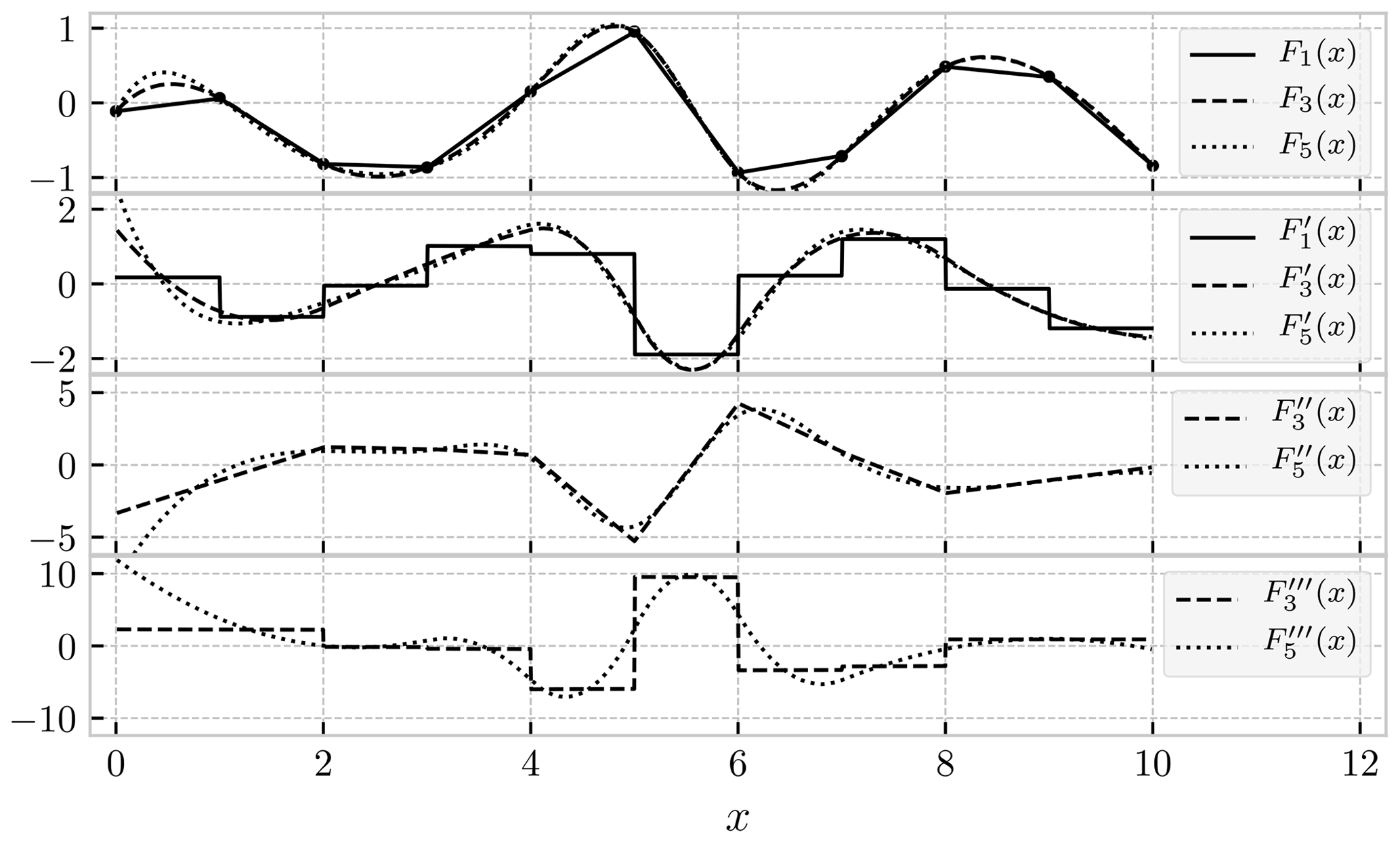
Figure 1 One-dimensional illustration of different degrees of interpolation. From the same 11 data points (shown as black circles in the top panel), we have constructed a linear interpolation (continuous lines), a cubic spline interpolation (dashed lines), and a quintic spline interpolation (dotted lines). From the top, the panels show the interpolated functions, the first derivative, the second derivative, and the third derivative. We observe that linear interpolation, F₁(x), gives a discontinuous derivative, and cubic interpolation, F₃(x), gives a discontinuous third derivative.

To aid the later discussion, we will briefly explain spline interpolation in one dimension. The generalisation to higher dimensions is natural. Assume that we have a grid of N equidistant points, $x_n\in \mathit{\{}{x}_{\mathrm{1}},x_{\mathrm{2}},\mathrm{\dots },x_{N-\mathrm{1}},x_N\mathit{\}}$, and the values of some function in those points, y_n=f(x_n). The aim of an interpolation procedure is to allow us to approximate the function f(x) at arbitrary x, subject to $x_{\mathrm{1}}\le x\le x_N$. In the case of linear interpolation, the value of the linearly interpolated function F₁(x) on the interval $[x_n,x_{n+\mathrm{1}}]$ is given by

$$\begin{array}{}\text{(14)}& F_{\mathrm{1}}\left(x\right)=f\left(x_n\right)+{\displaystyle \frac{x-x_n}{\mathrm{\Delta }x}}\cdot \left(f\left(x_{n+\mathrm{1}}\right)-f\left(x_n\right)\right),\end{array}$$

where $\mathrm{\Delta }x=x_{n+\mathrm{1}}-x_n$ is the grid spacing. We see that F₁(x) is a continuous function, but its derivative, $F_{\mathrm{1}}^{\prime }\left(x\right)$, is not continuous at the grid points. A cubic spline interpolation, F₃(x), of the same data points as above will be given on an interval $[x_n,x_{n+\mathrm{1}}]$ by a cubic polynomial, e.g.

$$\begin{array}{}\text{(15)}& F_{\mathrm{3}}\left(x\right)=w_{\mathrm{0}}+w_{\mathrm{1}}\stackrel{\mathrm{̃}}{x}+w_{\mathrm{2}}{\stackrel{\mathrm{̃}}{x}}^{\mathrm{2}}+w_{\mathrm{3}}{\stackrel{\mathrm{̃}}{x}}^{\mathrm{3}},\end{array}$$

where $\stackrel{\mathrm{̃}}{x}=x-x_n$ and the weights, w₀, w₁, w₂, and w₃ are chosen such that F₃(x), $F_{\mathrm{3}}^{\prime }\left(x\right)$, and $F_{\mathrm{3}}^{\prime \prime }\left(x\right)$ are all continuous at the grid points (see, e.g. Press et al., 2007, pp. 120–124). By the same token, a fifth-degree spline interpolation gives a piecewise polynomial function of degree 5, with the property that the first, second, third, and fourth derivatives are continuous at the grid points. A one-dimensional illustration of the three degrees of interpolation considered in this paper is provided in Fig. 1. For a description of how spline interpolation of ocean current velocity fields was implemented, see Sect. 4.

Finally, we would like to note two important points on the subject of interpolation in Lagrangian oceanography. First, the purpose of interpolating discrete current data is not to approximate the unresolved turbulent motion of the ocean but simply to provide a consistent recipe for evaluating gridded data at arbitrary locations. Second, once an interpolation scheme has been chosen, one has effectively replaced the gridded input data by a set of analytical expressions, specifying a way in which to evaluate the velocity field at any point and time. Hence, for a given dataset and interpolation scheme, the initial value problem given by $\dot{\mathit{x}}=\mathit{v}(\mathit{x},t)$, x(t₀)=x₀, has a unique true solution (provided the usual conditions for existence and uniqueness of solutions of ODEs are met; see, e.g. Hairer et al., 1993, pp. 35–43). With an increasingly short time step, h→0, stable and consistent numerical integration schemes should converge towards the true solution. However, velocity fields evaluated with different orders of interpolation are not identical, and will not produce identical trajectories, even as h→0.

3 Special-purpose integrators

In this section, we will discuss the implications of our ODE having a right-hand side with discontinuous derivatives. We consider an analytical example with one discontinuity to illustrate the problem and present a modified special-purpose integration routine that handles the discontinuity. We then describe how to implement the same idea in special-purpose variants of regular variable-step integrators for application in Lagrangian oceanography.

3.1 Discontinuous derivatives

As mentioned in Sect. 2.1, the conditions for a pth-order Runge–Kutta method to actually be pth-order accurate, require continuous derivatives of the right-hand side, up to and including order p. The problem is that consistency of order p of the numerical method is no longer satisfied when the derivatives are not continuous (Kress, 1998, pp. 235, 252). In many cases this means that the error is larger than expected, but in some cases the problem may be more serious: the numerical approximation may be meaningless (Isaacson and Keller, 1994, p. 346). The more pathological examples are perhaps unlikely to occur in practice. However, as we will see later, when the error in even a single step is unbounded by Eq. (7), this can in some cases dominate the global error, rendering the use of a higher-order scheme pointless.

In practical applications, with interpolated velocity fields, the derivatives are not always continuous. For example, a common choice in the LCS literature appears to be a variable-time-step integrator of order 4 and 5 (see, e.g. Ali and Shah, 2007; Shadden et al., 2010; Beron-Vera et al., 2010; Maslo et al., 2020). Theoretically, seventh-order spline interpolation, yielding five continuous derivatives, is required for the error estimates in the step size control routine to hold. However, higher-order spline interpolation is more computationally demanding, and in practice cubic spline interpolation appears to be a common choice. It is also worth noting that, in general, spurious oscillations become increasingly problematic with increasing spline order.

For such cases, strategies exist to deal with the discontinuities in the right-hand side or (more commonly in our case) its derivatives (Hairer et al., 1987, p. 181). Three possible strategies for dealing with ODEs with discontinuities are outlined by Hairer et al. (1993, pp. 197–198).

• i.

  Ignore the discontinuity, and let the variable-step-size integrator sort out the problem.

• ii.

  Use an integrator with an error control routine specifically designed to detect and handle discontinuities (see, e.g. Enright et al., 1988; Dieci and Lopez, 2012).

• iii.

  Use information about the position of the discontinuity to stop and restart integration at that point.

Given that the issue of interpolation and integration is not typically discussed in great detail in applied papers on Lagrangian oceanography, one assumes that most authors implicitly select the first strategy. However, as pointed out by Hairer et al. (1987, p. 181), this is neither the most accurate nor the most numerically efficient approach.

3.2 Analytical example

To illustrate the effect of discontinuities in the derivative of the right-hand side, we consider the following ODE:

$$\begin{array}{}\text{(16)}& \dot{x}=\left|\sin \left(\mathit{\pi }t\right)\right|,x(t=\mathrm{0})=\mathrm{0}.\end{array}$$

In this case, the right-hand side itself is continuous, but its derivative is discontinuous at t=1. This equation has the following analytical solution:

$$\begin{array}{}\text{(17)}& x\left(t\right)=\underset{\mathrm{0}}{\overset{t}{\int }}\left|\sin \left(\mathit{\pi }s\right)\right|\mathrm{d}s,\end{array}$$

and if we consider the solution at time t_N=2 as an example, we find $x\left(t_N\right)=\mathrm{4}/\mathit{\pi }$. Since the exact solution is known, we can find the error in our numerical solutions by using the exact result as a reference. Hence, we can investigate the convergence of our numerical integration scheme by considering the error as a function of the time step, h.

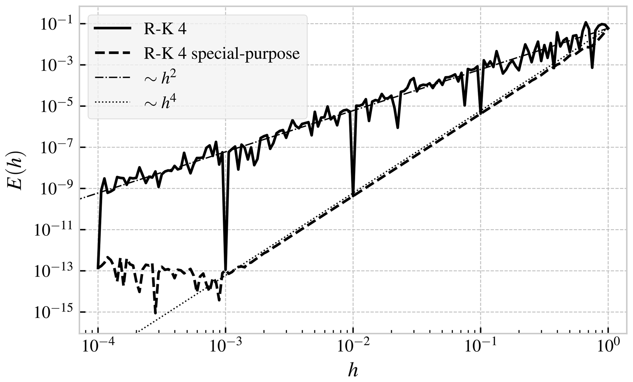
Figure 2 Global error in the numerical solution of the initial value problem given by Eq. (16) at t_N=2. The solutions have been calculated with 161 different time steps, h, logarithmically spaced from 10⁻⁴ to 1, using the fourth-order Runge–Kutta integrator and a special-purpose modification of the same that stops and restarts the integration exactly at the discontinuity at t=1. The two thin lines are included to indicate the order of convergence and are proportional to h² (dashed–dotted line) and h⁴ (dotted line).

In Fig. 2, we show the global error in the solution as a function of time step, h, for the fourth-order Runge–Kutta integrator (continuous black line). The error has been calculated for 161 logarithmically spaced time steps from 1 to 10⁻⁴. Of these 161 time steps, only 1, 10⁻¹, 10⁻², 10⁻³, and 10⁻⁴ will evenly divide an interval of length 1. This is significant, as we observe that the error scales approximately as h⁴ for the time steps 1, 10⁻¹, 10⁻², and 10⁻³, while for the other time steps it follows a slower h² scaling. (Note that at $h={\mathrm{10}}^{-\mathrm{4}}$, the error is dominated by roundoff error (see Appendix A1), which adds up to about 10⁻¹³ after 20 000 steps; Press et al., 2007, p. 10.)

The reason for this behaviour is the discontinuity at t=1. For those time steps that divide an interval of length 1 into an integer number of steps, the integration will be stopped and restarted exactly at the discontinuity in the derivative of the right-hand side at t=1. Therefore, the error bound (Eq. 7) holds, since the method does not step across the discontinuity. Stopping and restarting at discontinuities is precisely what Hairer et al. (1993, pp. 197–198) recommends in strategy iii discussed in Sect. 3.1 above, and in this sense, isolated discontinuities in the derivatives are easy to handle if it is known where they are a priori.

Inspired by this result, we have designed a special-purpose version of the fourth-order Runge–Kutta integrator, specifically for this problem with a discontinuity at t=1. It is identical to the regular one in every way, except that if $t<\mathrm{1}<t+h$, it divides that step into two steps of length 1−t and $h-(\mathrm{1}-t)$, such that the integration is always stopped and restarted at t=1.

The global error as a function of time step for this special-purpose integrator is also shown in Fig. 2 (dashed line), and we observe that it follows the expected h⁴ scaling very closely until the point where round off error starts to dominate. The additional computational expense of the special-purpose integrator is completely negligible in this case, as it takes at most one additional step compared to the regular fourth-order Runge–Kutta method, but as we see, it can increase the accuracy by several orders of magnitude. In the next section, we apply this idea to variable-time-step integrators for trajectory calculation in interpolated vector fields.

3.3 Special-purpose integrators for interpolated velocity fields

In terms of the three strategies for dealing with discontinuities (see Sect. 3.1) we will investigate a hybrid approach in this paper. We will use information about the location of the discontinuities in the time dimension (strategy iii) and leave the error control routine to deal with the problem in the spatial dimensions (strategy i). The reason for this choice is mainly pragmatic: for a particle trajectory, x(t), time is the independent variable, and it is very easy to stop and restart integration at “cell boundaries” in the time direction. Doing the same in the spatial dimensions requires detection of boundary crossings, dense output from the integrator, and a bisection scheme to identify the time at which the boundary is crossed (Hairer et al., 1993, pp. 188–196).

We will take as our starting point variable-time-step Runge–Kutta methods, as these are commonly used and generally quite efficient, and the time step adjustment routine outlined in Sect. 2.3. We then modify the time step adjustment routine to make sure the integration is always stopped and restarted at a cell boundary in time. We assume that the input data is given as snapshots of a vector field at a list of known times, T_i. Depending on the degree of interpolation, the (higher) partial derivatives of the interpolated vector field along the time dimension will thus have discontinuities at times T_i.

The variable-time-step integrator calculating the trajectory will make steps, from position x_n, at time t_n, to position x_n+1, at time $t_{n+\mathrm{1}}=t_n+h_n$. Then, if we have $t_n<T_i<t_n+h_n$, for any T_i, i.e. if the integration is about to step across a discontinuity in time, the time step, h_n, is adjusted such that

$$\begin{array}{}\text{(18)}& h_n=T_i-t_n.\end{array}$$

After that, integration and error control proceeds as normal. If h_n is set to T_i−t_n, then a step to that time is calculated. The error is then checked, as described in Sect. 2.3. If the error is found to be too large according to the selected tolerance, the step is rejected, h_n is further reduced, and the step is attempted again. In the opposite case, the step is accepted, and time and position is updated to t_n+1 and x_n+1. At this point, the time step is reset to the original value of h_n to avoid the integration proceeding with an unnecessarily short time step after the discontinuity has been crossed. For any step that does not cross a discontinuity in time, the integrator behaves exactly like the regular version.

4 Numerical experiments

The aim of the numerical experiments is to investigate the practical implication of different combinations of interpolation and integration schemes and to compare the special-purpose integrators described in Sect. 3.3 with their standard counterparts, as well as with fixed-step Runge–Kutta methods. In the following subsections, we describe the input data and the setup used to carry out the numerical experiments. We have chosen to consider two-dimensional (horizontal) transport only, using the surface layer of the modelled current data. The current velocity field is interpolated in three dimensions (two spatial dimensions plus time), using the same degree of interpolation in all three dimensions.

In order to allow the interested reader to reproduce our results, we provide the Fortran code used to run the simulations, the ocean current data used, and the Jupyter notebooks that were used to analyse the data (Nordam, 2020). These can all be found on GitHub¹ under an open-source license. In order to reduce the file size of the current data, the extents of the original datasets were reduced, and unused variables were deleted from the files. The domains of the reduced datasets are shown in Fig. 3. All of the datasets were originally downloaded in the netCDF format from the ocean and ice section of the THREDDS server of the Norwegian Meteorological Institute².

4.1 Ocean currents

The datasets used were obtained from the Norwegian Meteorological Institute, and were taken from the following model setups:

• -

  Arctic20km (20 km horizontal resolution, 1 h time step),

• -

  Nordic4km (4 km horizontal resolution, 1 h time step),

• -

  NorKyst800m (800 m horizontal resolution, 1 h time step).

The dimensions of the datasets are x, y, z, and t, with the xy plane defined in a polar stereographic projection, giving a regular (constant spacing) quadratic grid in the horizontal plane. The current velocity field is provided as vector components on the xy basis (as opposed to, e.g. an east–north basis). In our simulations, we track particle positions in metres, using the xy coordinate system of the polar stereographic projection of the datasets. This allowed us to use the vector components directly from the datasets, with no rotation or other conversion. All error measurements are calculated from Euclidean distances in the xy plane.

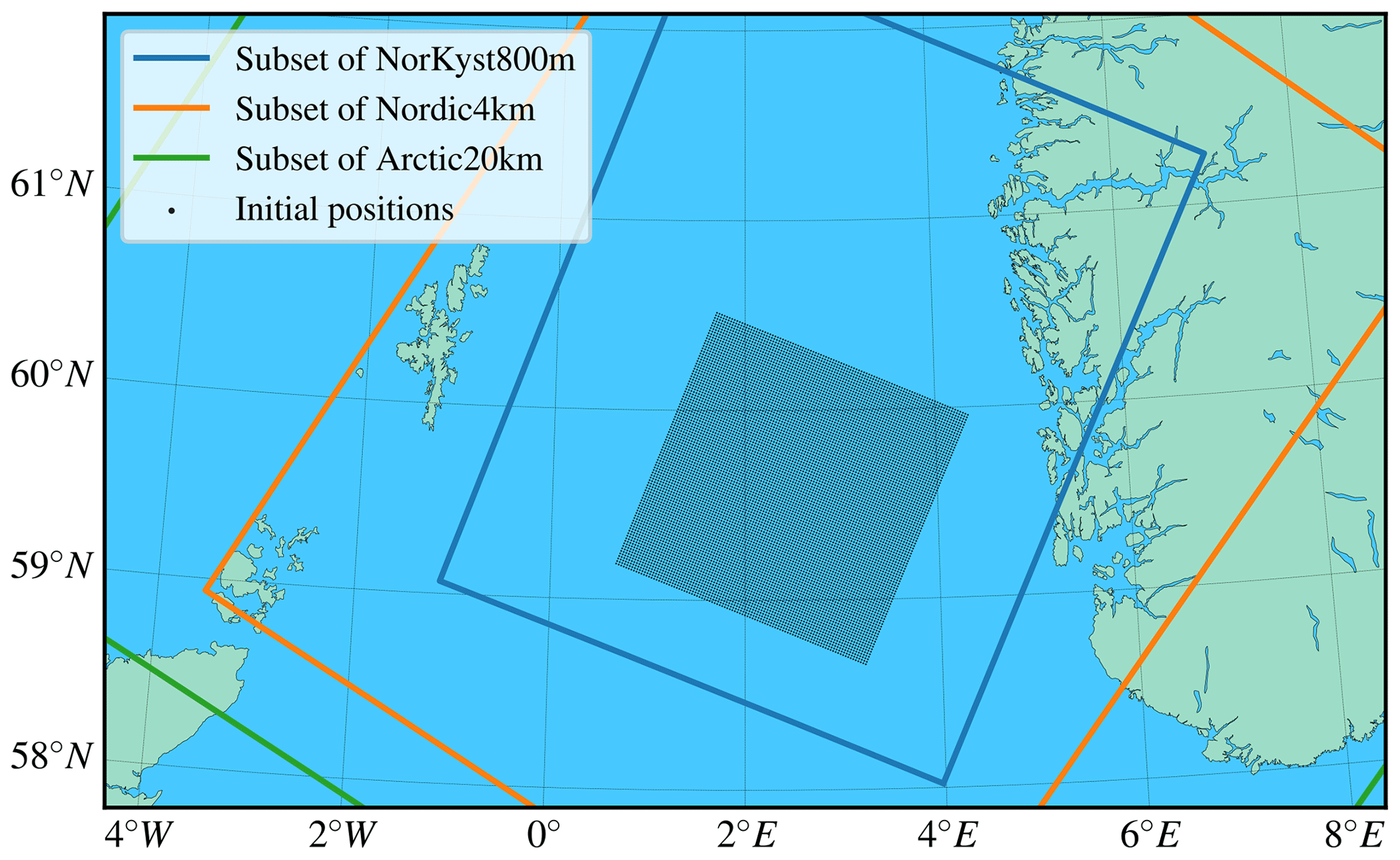
Figure 3 Map showing the outline of the three datasets considered, as well as the initial positions of the tracers used in the numerical experiments.

4.2 Initial conditions

The initial conditions for the trajectory calculations were chosen to be 100×100 points off the coast of Norway, placed on a regular quadratic grid with grid spacing of 1600 m, as shown in Fig. 3. The same initial conditions were used for all three datasets. Roughly the easternmost half of the initial positions are within the Norwegian coastal current (see, e.g. Sætre, 2005) and are predominantly transported northward along the coast. The trajectories were started at midnight on 8 February 2017 and integrated for 72 h. All the particles remain inside the smallest domain (the 800 m resolution setup; see Fig. 3) throughout this period. The final positions are shown in Fig. 4 for each of the three different datasets.

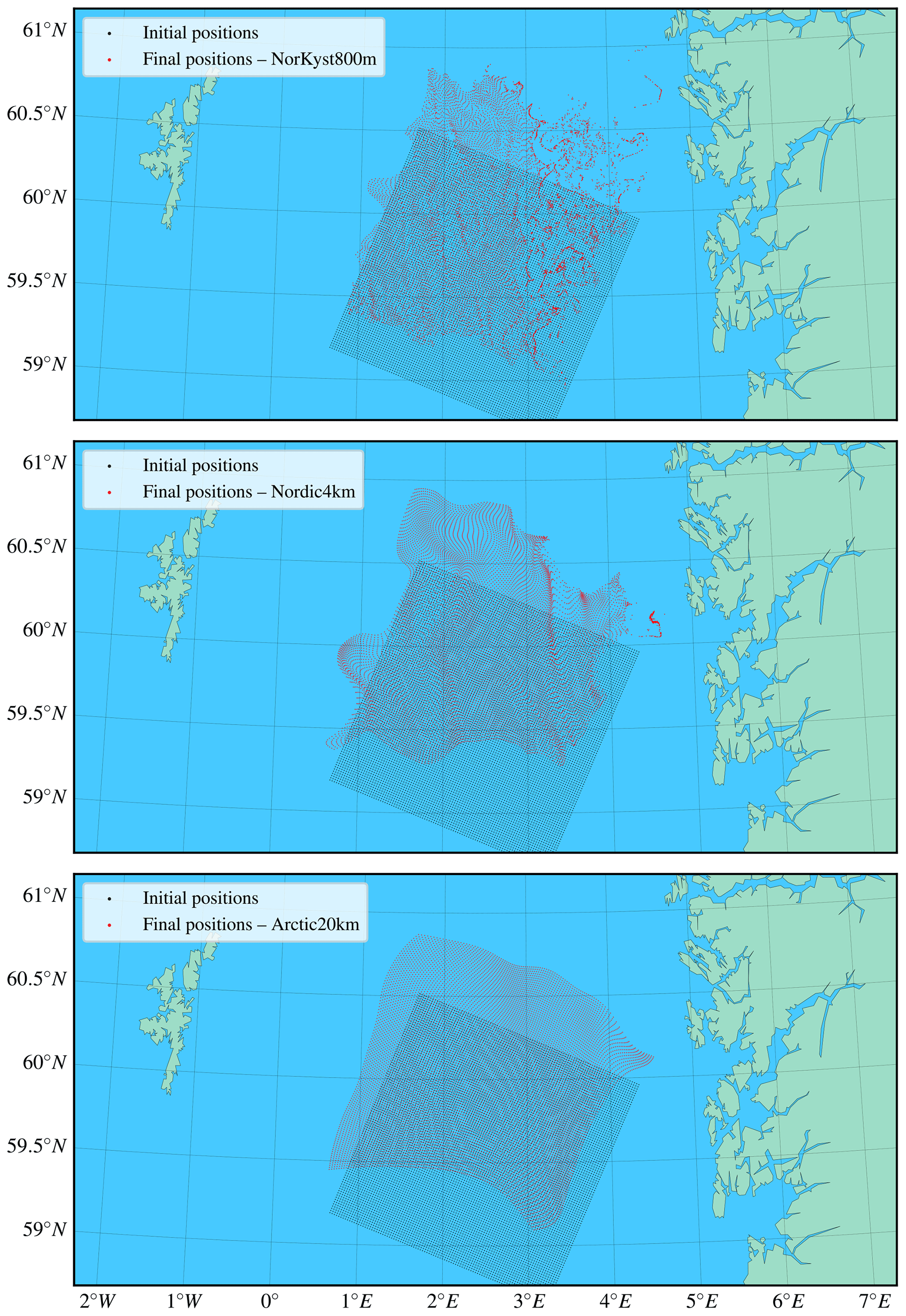
Figure 4 The figure shows the initial and final positions of the 10 000 particles for the three different datasets. The initial positions are the same, but the final positions differ. The average transport is towards the north in all cases, but the higher-resolution currents show more eddy activity, particularly in the eastern region, which falls within the Norwegian Coastal Current (see, e.g. Sætre, 2005). These plots show the positions calculated with cubic interpolation, fourth-order Runge–Kutta, and a time step of 1 s. Results obtained with the other methods appear visually identical at this scale.

4.3 Reference solutions

As we wish to estimate the global error of our numerical solutions, when the true solutions are unknown, we need to establish highly accurate numerical solutions for all 10 000 initial conditions to use as a reference. Reference solutions must be established for each dataset, as they will in general give different trajectories. Additionally, reference solutions must also be established for each interpolation scheme, as they will also in general give different trajectories. Hence, for three datasets and three interpolation schemes, we need nine different sets of reference solutions.

We point out that we here talk about reference solutions in a purely numerical sense, as the most mathematically accurate solution of the initial-value problem given by an initial position and a discrete velocity field with a specified interpolation scheme. Which of the datasets and interpolation schemes that most accurately reproduce the trajectories of true Lagrangian drifters in the ocean is a different question, outside the scope of this investigation.

For numerically obtained reference solutions to be useable in calculating error estimates, they need to be significantly more accurate than any of the numerical solutions that are to be evaluated. As an example, consider a fixed-step integrator and let the numerical solution at time t_N, calculated with a time step h, be x_N(h) and let the true (but usually unknown) solution at time t_N be x(t_N). Furthermore, assume that a reference solution x_N(h_ref) has been calculated with a very short time step h_ref.

Then, the error in the reference solution, relative to the true (but unknown) solution, is given by

$$\begin{array}{}\text{(19)}& E_{\mathrm{ref}}={\mathit{x}}_N\left(h_{\mathrm{ref}}\right)-\mathit{x}\left(t_N\right).\end{array}$$

Similarly, the error in a solution calculated with a longer time step, h, is

$$\begin{array}{}\text{(20)}& E\left(h\right)={\mathit{x}}_N\left(h\right)-\mathit{x}\left(t_N\right).\end{array}$$

When we estimate the error by purely numerical means, we do not know the true solution, x(t_N). Instead, we use the reference solution in place of the true solution, and calculate an estimate of the error, given by

$$\begin{array}{}\text{(21)}& \begin{array}{rl}\stackrel{\mathrm{‾}}{E}\left(h\right)& ={\mathit{x}}_N\left(h\right)-{\mathit{x}}_N\left(h_{\mathrm{ref}}\right),\\ & =E\left(h\right)-E_{\mathrm{ref}}.\end{array}\end{array}$$

Hence, we see that the numerical estimate, $\stackrel{\mathrm{‾}}{E}\left(h\right)$, of the global error, is only a good estimate if E_ref≪E(h).

To verify that the errors in the reference solutions are indeed much smaller than any of the other errors we wish to estimate, we consider the convergence of the numerically estimated error. The details of the analysis to identify reference solutions are shown in Appendix A. We found that the most accurate solutions were obtained with the fourth-order Runge–Kutta integrator, using a fixed short time step. The time step that yielded the most accurate solutions varied, depending on the dataset and the order of interpolation. The results are given in Table A2.

4.4 Implementation

To allow easy testing of different combinations of datasets, interpolators, and integrators in a setting relevant for marine transport applications, a simple Lagrangian particle transport code was written in Fortran. All the integrators were implemented as described in Sects. 2.2, 2.3, and 3.3 and in the references given. The netCDF library for Fortran³ was used to read ocean current data, and interpolation was done using the library bspline-fortran⁴ (Williams, 2018). Our implementations of the different integrators, and all the code used to run the simulations, are freely available on GitHub⁵.

At the start of the simulations, subsets of the ocean current datasets were loaded from file. The horizontal extent of the subsets are shown in Fig. 3, along with the initial positions of the particles. We used only the surface layer of the datasets and data spanning 5 d. The subsets were selected to cover the entire simulation period in time and the entire horizontal extent of the particle trajectories, extending some cells in all directions to avoid edge effects in the spline interpolation. Data points that were on land were set to 0 current velocity. No special steps were taken to handle the coastline, although the initial conditions were chosen to avoid particles getting stuck in land cells. Note that with higher-degree interpolation schemes, the fact that we set the currents to zero in land cells will have an effect on one or more of the closest cells to the coastline. For applications such as oil spill modelling, where shoreline interactions are important, a different strategy might be needed.

The data were passed to the initialize method of the derived type bspline_3d from the bspline-fortran library, along with the parameter to select the order of interpolation (note that the order of a spline is 1 plus the polynomial degree, meaning the order is 2 for linear interpolation, 4 for cubic splines, and 6 for quintic splines). The x and y components of the current velocity vectors were interpolated separately, and the order of interpolation was always the same along all three dimensions (x, y, t).

We note that this approach constructs a single global interpolation object, that is used throughout the simulation. It is also possible to construct local spline interpolations using only the smallest required number of points, surrounding the location where the function is to be evaluated ($\mathrm{2}\times \mathrm{2}\times \mathrm{2}$ points for linear interpolation, $\mathrm{4}\times \mathrm{4}\times \mathrm{4}$ for cubic splines, and $\mathrm{6}\times \mathrm{6}\times \mathrm{6}$ for quintic). However, this creates additional discontinuities in the derivatives of the right-hand side when switching from one local interpolator to the next, as discussed by, e.g. Lekien and Marsden (2005).

During the simulations, the trajectory of each particle was calculated independently of all others. For the variable-step integrators, this means that each particle had its own time step. It is also possible to apply the variable-step integrators to all particles simultaneously with the same time step. However, due the local variability of the ocean currents, it seemed more reasonable to treat the particles individually, allowing the variable-step integrators to adapt to local conditions for each particle.

5 Results and discussion

The main results are presented as a work–precision diagram, in Fig. 5. The figure shows the median relative global error over all 10 000 particles, as a function of number of evaluations of the right-hand side of the ODE (including rejected steps). The relative global error is calculated as the normalised distance between the endpoint of each trajectory and that of the corresponding reference solution (see Sect. 4.3 and Appendix A). See also Fig. B1, where the range of errors is shown.

Number of evaluations of the right-hand side was chosen as a measure of work, as it is more objective than the runtime of the simulation, which would depend on the particular machine used to run the simulations and also be more susceptible to somewhat random variations. However, for the interested reader we show the error as a function of runtime in Fig. B2.

While we analyse the results in terms of number of function calls, we note that higher-degree interpolation is more computationally costly than lower-degree interpolation. This means that the same number of evaluations will take more time if a higher degree of interpolation is used. We found that for the simulations done with the fixed-step fourth-order Runge–Kutta integrator, the simulations with cubic spline interpolation took on average four to five times longer than those with linear interpolation, and the simulations with quintic spline interpolation took on average three to four times longer than those with cubic spline interpolation. As a concrete example, calculating the trajectories of 10 000 particles for 72 h with a 10 min time step with the fourth-order Runge–Kutta integrator, took 11 s with linear interpolation, 51 s with cubic interpolation, and 177 s with quintic interpolation. The numbers were essentially the same for all three datasets (800 m, 4 km and 20 km). These times cover only the trajectory calculation itself, not file I/O or the construction of the global interpolator object.

The fixed-step integrators were run with the range of time steps shown in Table 1. Note that all of these steps evenly divide the 3600 s interval of the data, making sure that the integration is always stopped and restarted at a cell boundary in the time dimension (see discussion in Sect. 3).

Table 1 Time steps and tolerances used in the numerical experiments.

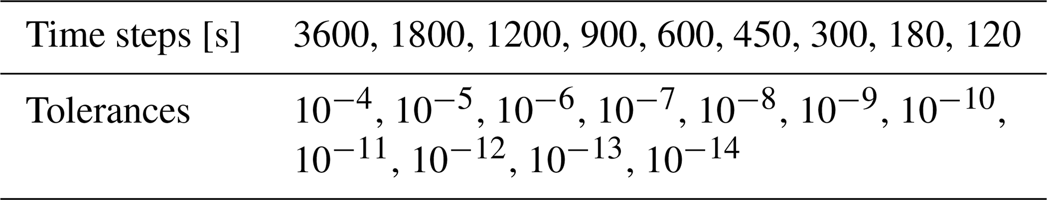
The tolerances used with the variable-step integrators are also shown in Table 1, with T_A=T_R (see Sect. 2.3). Note that in the coordinate system used, the particle positions are all of the order 10⁶ m, meaning that the relative tolerance dominates in practice (see Eq. 10). Both the regular and the special-purpose variable-step integrators were used with the same tolerances, but we note that the special-purpose integrators are by design unable to take steps longer than the interval on which the data is given. Hence, for the higher tolerances (allowing larger errors), the special-purpose integrators would default to fixed-step integration with a time step of 3600 s (for the datasets used here).

We observe from Fig. 5 that the most efficient choice of integrator, in the sense of fewest evaluations of the right-hand side for a given accuracy, depends on the desired accuracy, the order of the interpolation, and the spatial resolution of the dataset. We will discuss these points in turn.

Figure 5 Relative global error (relative to the reference solution) as a function of number of evaluations of the right-hand side. Note that the special-purpose integrators are (by design) unable to make longer steps than the interval on which the data are provided. This means some of the simulations with higher tolerance (allowing larger errors) have in practice defaulted to fixed-step simulation with a time step of 3600 s, making several of the data points identical. This is most readily observed for the special-purpose Dormand–Prince 8(7) integrator in the lower-right panel.

5.1 Fixed-step integrators

Variable-step integrators are normally the most efficient choice for general ODE problems. However, we see that for finding tracer trajectories from interpolated velocity fields, fixed-step integrators are in some cases a better choice than regular variable-step methods. Considering for example cubic spline interpolation (Fig. 5, middle row), we see that fourth-order Runge–Kutta almost always gives better accuracy for the same amount of work, relative to all three regular variable-step integrators. The only exception is for very small errors, for the 800 m dataset, where Dormand–Prince 5(4) has a small advantage. Similarly, for linear interpolation (Fig. 5, top row) the third- and fourth-order fixed-step methods outperform the regular variable-step methods, except if very small errors are required.

The special-purpose variants of the variable-step integrators, particularly Dormand–Prince 5(4) and 8(7), perform better than the fixed-step methods in most cases, though not always by a large margin. The reason for the relatively strong performance of the fixed-step integrators is that the chosen time steps evenly divide the 3600 s intervals of the datasets. Hence, the fixed-step integrators will stop and restart integration at the discontinuities in time, just like the special-purpose integrators (see Sect. 3.3). For an illustration of the effect of choosing time steps that do not evenly divide the temporal grid spacing of the dataset, see Nordam et al. (2017, Fig. 18).

We also note that for the case of linear interpolation, the third-order Runge–Kutta integrator actually performs slightly better than the fourth-order integrator, particularly for the smaller errors. The reason for this is that the lack of continuous derivatives means the fourth-order method does not achieve fourth-order convergence. As the third-order method uses one fewer evaluation of the right-hand side per step, it therefore has an advantage in terms of computational effort. It is also worth pointing out that the second-order Runge–Kutta method considered here, known as the explicit trapezoid method, has the advantage that it uses no intermediate points in time. Since it only evaluates the right-hand side at times t_n and t_n+1, it is possible to dispense with interpolation in time entirely if one selects the integration time step, h, to be equal to the temporal grid spacing of the data. Note that this requires reasonably high temporal resolution of the dataset, which may not always be practical.

5.2 Variable-step integrators

As a background for discussing the effect of horizontal resolution on our results, we recall that all the three datasets used have a temporal resolution of 1 h. This means that the particle trajectories will cross a cell boundary in the time-dimension (and thus a discontinuity in the (higher) derivatives of the right-hand side) every hour. The average current speed for the time and area studied is approximately 0.2 m s⁻¹ in all three datasets. Hence, we find that a particle that moves in the velocity field defined by the dataset at 800 m spatial resolution will cross a spatial cell boundary approximately once every hour on average. For the dataset with 4 km resolution, this will only happen 1/5th as often, and for the 20 km dataset this will only happen 1/25th as often. These are only crude estimates, but we can nevertheless conclude that for the low-resolution datasets, the errors picked up at the discontinuities in time will be more important than those in space, while for the high-resolution (800 m) dataset, the two will be of similar importance.

Looking at the results presented in Fig. 5, we find that they support these observations. Considering first the case of linear interpolation, we see that for the 20 km dataset (Fig. 5, upper-right panel), there is a considerable (several orders of magnitude) reduction in error in the special-purpose integrators compared to the regular variable-step integrators for a given number of evaluations. Recall that the only difference between these is that the special-purpose integrators stop and restart the integration at every cell boundary along the time dimension (see Sect. 3.3). For the 800 m dataset (Fig. 5, upper-left panel) on the other hand, there is less (up to about an order of magnitude) difference between the regular and special variable-step integrators. This is presumably because the discontinuities in time do not dominate the error as much in this case.

Looking next at the results for cubic spline interpolation (Fig. 5, middle row), we notice that the results for the regular and special-purpose versions of the Bogacki–Shampine 3(2) integrator are now practically identical. For the Dormand–Prince 5(4) and 8(7) integrators, the special-purpose variants are far more accurate than the standard counterparts. This is particularly true for the 4 and 20 km datasets, where the difference is several orders of magnitude.

Presumably, the reason why the standard and special-purpose variants of the Bogacki–Shampine 3(2) integrator give more or less identical results for cubic interpolation is the smoothness of the velocity field. It seems the interpolated field is now sufficiently smooth that the method is now third-order consistent. Strictly speaking, this is unexpected. A cubic spline interpolation will have continuous second derivatives, and discontinuous third derivatives. This means that the Bogacki–Shampine 3(2) integrator can indeed be expected to be second-order consistent, but the conditions for the third-order consistency are not satisfied.

Using quintic spline interpolation (Fig. 5, bottom row), the special-purpose variant of the Dormand–Prince 8(7) integrator performs better than all the other methods by at least an order of magnitude. We also find that the results for the regular and special-purpose versions of the Dormand–Prince 5(4) integrators are more or less identical. As above, this was not entirely expected, since a quintic spline has only four continuous derivatives, not the five that are theoretically required for the local error of a fifth-order method to be bounded by Eq. (7).

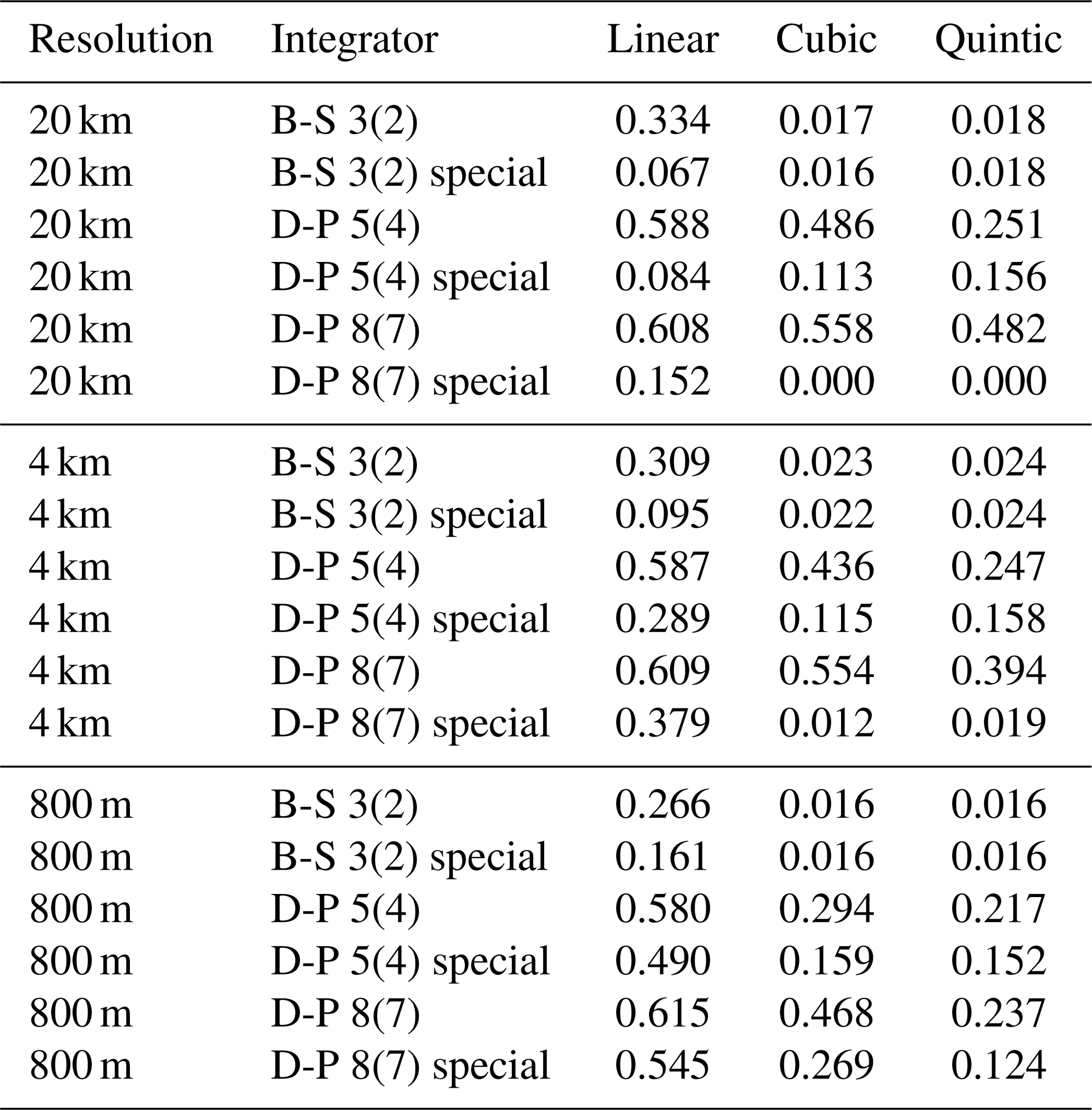
To understand the large differences in number of function evaluations between the standard and the special-purpose integrators, we look at the fraction of rejected steps. For the different integrators and interpolators, and a fixed tolerance of $T_{\mathrm{A}}=T_{\mathrm{R}}={\mathrm{10}}^{-\mathrm{10}}$, these fractions are given in Table 2. Rejected steps represent wasted computational effort, since a rejected step requires as many evaluations of the right-hand side of the ODE as an accepted step, without advancing the integration.

The results shown in Table 2 further support the conclusions we drew from Fig. 5 above. For those cases where the order of interpolation is less than the theoretical requirements of the integrator, the special-purpose integrators significantly reduce the fraction of rejected steps. The difference is also largest for the 20 km dataset, as discussed previously. This can be seen particularly for the Dormand–Prince 8(7) integrator with cubic and quintic interpolation, where the rejected fraction falls to almost nothing for the special-purpose variant. The same, but to a lesser degree, is seen for the Dormand–Prince 5(4) integrator, with linear and cubic interpolation. On the other hand, for the Bogacki–Shampine 3(2) integrator, with cubic and quintic interpolation, we see that there is essentially no difference between the regular and special variants, as the velocity field is sufficiently smooth for the error control routine not to detect any increased local error at the boundary crossings.

The largest improvement in accuracy for the special-purpose integrators is thus seen with linear interpolation, but they can also be advantageous with cubic interpolation. With quintic interpolation, only the special-purpose (8)7 integrator has an advantage over its regular counterpart. However, the relative error of the special (8)7 method with quintic interpolation is comparable to the (5)4 method with cubic interpolation. While the solutions will be different with different interpolation schemes, it is possible that overshooting due to a high-order interpolation method without any additional accuracy implies that the (8)7 method is not a good choice for Lagrangian oceanography. Note also that the quintic interpolation scheme is 3–4 times as computationally expensive as the cubic scheme for each evaluation of the right-hand side.

Table 2 Fraction of steps rejected, averaged over all 10 000 trajectories, with a duration of 72 h, for each combination of interpolation scheme and variable-step-size integrator, for all three datasets and a fixed tolerance of $T_{\mathrm{A}}=T_{\mathrm{R}}={\mathrm{10}}^{-\mathrm{10}}$ (see Sect. 2.3).

5.3 Diffusion

As mentioned in Sect. 2, we have considered pure advection, ignoring diffusion. Calculating trajectories with pure advection by a deterministic velocity field is common in several applications, perhaps most notably for identification of LCS (see, e.g. Haller, 2015; Allshouse et al., 2017; Duran et al., 2018). Other examples include the use of backwards trajectories to identify source regions for particles ending up in the sediments (van Sebille et al., 2015) and analysis of Lagrangian pathways to study the source and history of water parcels reaching a particular upwelling zone (Rivas and Samelson, 2011). In general, simulating diffusion in Lagrangian oceanography (or meteorology) may introduce a complication that encourages some studies to compute trajectories without diffusion: Lagrangian motion becomes ambiguous when diffusive mixing is simulated because the identity of a fluid parcel is lost. On the other hand, ignoring small-scale mixing may also be problematic. One approach to this problem is to supplement purely advective trajectories with along-path changes in parcel properties, as discussed in Rivas and Samelson (2011).

However, for many other applications diffusion must be included. Solving the advection-diffusion equation with a particle method amounts to numerical solution of a stochastic differential equation (SDE) instead of an ODE. A range of different SDE schemes exist, and the details differ, but all such schemes involve adding a random increment at each time step. If the random increment is far larger than the local numerical error in each step, then the numerical error in the advection is probably of limited practical importance. The details will depend on the application, and we encourage experimentation. A detailed description of numerical SDE schemes is outside the scope of this study, but the interested reader may find it useful to refer to, e.g. Kloeden and Platen (1992), Spivakovskaya et al. (2007), and Gräwe (2011).

5.4 Summary

We have seen that the special-purpose integrators are more efficient than their regular counterparts in almost all cases, and sometimes they deliver several orders of magnitude improvement in accuracy at the same computational cost. There are two different effects that give the special-purpose integrators their advantage in accuracy and efficiency. The first is that they stop and restart integration exactly at the discontinuities in time, which avoids picking up local errors unbounded by Eq. (7) at those points. The second effect is that they avoid many rejected steps by stopping at the discontinuity, instead of trying to step across.

The regular variable-step integrators will frequently try to step across a discontinuity, only to find that the estimated local error is too large, such that the step must be rejected and retried with a shorter time step. This process will continue until a time step is found that is short enough to allow the discontinuity to be crossed with an error that stays within the tolerance. As we see from the results in Table 2, this can lead to a large fraction of rejected steps. Also, recall that the regular variable-step integrators have no information about the location of the discontinuities in time, which means that the probability of stopping and restarting the integration exactly at a discontinuity is essentially zero. For further details, see the discussion in Sect. 3, as well as Hairer et al. (1987, p. 181) and Hairer et al. (1993, pp. 197–198).

6 Conclusions

In this paper, we have investigated how different numerical integrators behave in combination with different degrees of interpolation and datasets of different spatial resolution. We have calculated trajectories over 72 h, from 10 000 initial positions, and compared the integrator–interpolator pairs in terms of the error in the final position of each trajectory. We have considered linear, cubic, and quintic spline interpolation, along with four fixed-step Runge–Kutta integrators of orders 1 to 4, three commonly used variable-step integrators, and three special-purpose variants of the latter.

The most striking conclusion from our results is that the special-purpose integrators we describe in many cases deliver several orders of magnitude more accurate results at no additional cost. Alternatively, they can deliver the same accuracy as standard methods, with highly reduced computational effort. This is achieved by stopping and restarting the integration exactly at the grid points of the dataset along the time dimension. By doing this, we avoid stepping across discontinuities in the (higher) derivatives of the velocity field, and thus we avoid picking up local errors that are unbounded by Eq. (7) at those points.

The benefit is particularly visible for linear and cubic interpolation, and the 4 and 20 km datasets. The increased efficiency of these integrators should be particularly relevant for long-term simulations, such as studies of global transport of plastics or global climate simulations.

Going into more detail, we find that the most efficient choice of integrator depends on the resolution of the dataset, the degree of interpolation, and the desired accuracy. Looking at cubic interpolation (Fig. 5, middle row), we find that the fixed-step fourth-order Runge–Kutta method is in most cases a more efficient choice than a standard variable-step integrator (provided the time step is selected to evenly divide the interval of the dataset). The difference varies with the resolution of the dataset and the required accuracy, but in some cases the error is 2 orders of magnitude smaller for the fourth-order Runge–Kutta than the regular Dormand–Prince 5(4) method. This is an interesting result, given that the combination of cubic interpolation and a variable-step integrator such as Dormand–Prince 5(4) or Runge–Kutta–Fehlberg (Hairer et al., 1993, p. 177) appears to be a popular choice. In the case of the 20 km dataset, and to a lesser extent for the 4 km dataset, additional accuracy can be gained by switching to a special-purpose variant of the Dormand–Prince integrators.

For linear interpolation, we find that if very small errors are required, the regular variable-step integrators perform better than the fixed-step methods, particularly the Bogacki–Shampine 3(2) integrator. The special-purpose variable-step methods achieve notable improvements, often being several orders of magnitude more precise. For less strict requirements, the third-order Runge–Kutta method appears to be the best choice. However in all cases, there is a considerable improvement in accuracy with the special-purpose integrators relative to the regular variable-step methods.

For quintic spline interpolation, the optimal choice of interpolator again depends on the application. If very small errors are required, the Dormand–Prince 5(4) method appears to be the best performer, or alternatively the special-purpose variant of Dormand–Prince 8(7). If larger errors are acceptable, the fourth-order Runge–Kutta method seems to be the better choice.

It is interesting that if an appropriate fixed step is chosen (i.e. a step that divides the interval between discontinuities in time), the fourth-order Runge–Kutta method is more efficient than the regular Dormand–Prince (5)4 method for all ocean model resolutions. This is true for any interpolation scheme and accuracy, except linear and quintic interpolations when very small errors are desired. The fourth-order method with a good choice of time step also performs well relative to the special-purpose 5(4) method although the latter may significantly outperform the former with linear and cubic interpolations. The strong performance of the fourth-order Runge–Kutta with all resolutions and interpolation schemes makes it a good practical choice.

To conclude, we have investigated the accuracy of trajectory calculation with 10 different ODE integrators for 9 different combinations of current data resolution and order of interpolation. We find that the optimal choice of integrator depends on the interpolation, the resolution, and the required accuracy. In some cases, the most efficient integrator is not the most popular choice in the literature.

We have designed and investigated special-purpose variants of the regular variable-step integrators. Only minimal changes to the code is required to ensure that integration is always stopped and restarted at discontinuities in time. With this change, these special-purpose integrators can in some cases increase the accuracy by many orders of magnitude for the same amount of computational effort. For applications requiring large numbers of trajectories, such as LCS calculations, or for long-term transport calculations, the added accuracy of the special-purpose methods should allow significant reductions in computational expense.

Appendix A: Reference solutions

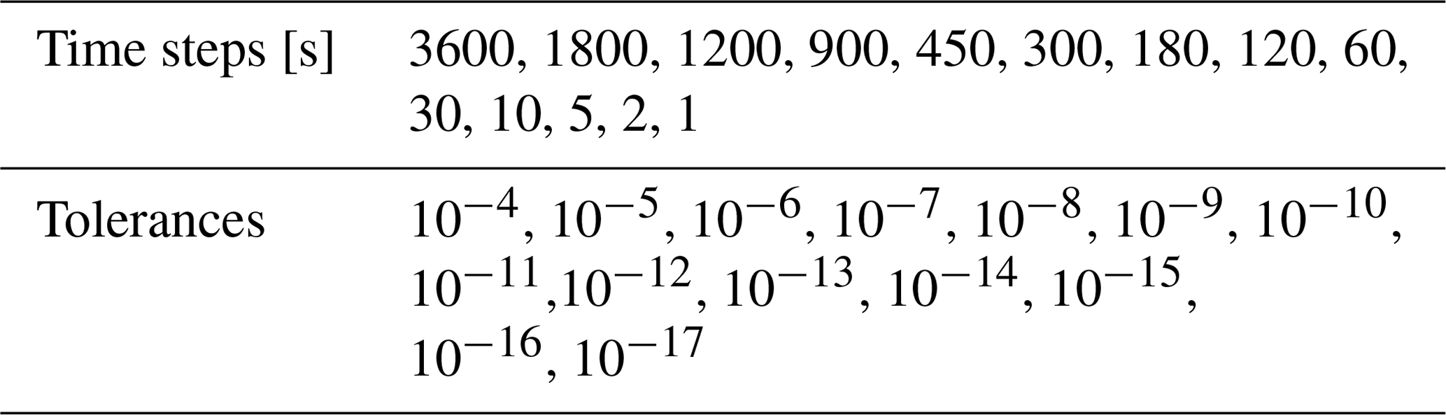
In order to establish highly accurate reference solutions, which are needed to estimate the error when the true solutions are unknown, an expanded set of time steps and tolerances were investigated. These are given in Table A1. For each time step in the expanded set, a solution was calculated with the fourth-order Runge–Kutta method, and for each tolerance in the expanded set, a solution was calculated with the Dormand–Prince 8(7) method, using both the regular and the special-purpose variant. This was done for each of the three datasets, and for each of the three orders of interpolation.

A1 Roundoff error and truncation error

Every step with a numerical ODE integrator contains some error. The truncation error stems from approximations that are made in constructing the integrator and decreases with time step. The round-off error comes from the finite-precision representation of numbers on a computer and is independent of the time step. Due to numerical round-off error, one can not simply assume that the shortest time steps or smallest tolerance will always give the most accurate answer. As the number of steps increase, the roundoff error will eventually become larger than the truncation error, at which point no accuracy is gained by reducing the step size further.

Loosely speaking, a double precision floating point number can store approximately 16 significant digits, and any numerical operation should be thought of as introducing a roundoff error in the least significant digit (Press et al., 2007, p. 10). This means that any step with an ODE integrator unavoidably introduces a relative error of approximately 10⁻¹⁶. As the time step is reduced, the numbers of steps increase, and eventually the net contribution of the added roundoff errors will dominate. An example of this can be seen in Fig. 2, where the error of the special-purpose method decreases down to about 10⁻¹³, whereafter it begins to increase with further reduction of the time step.

Table A1 Time steps and tolerances used in establishing reference solutions.

A2 Finding the most accurate solutions

In order to establish the most accurate solutions, we compare the fourth-order Runge–Kutta solutions obtained with very short time steps and Dormand–Prince 8(7) solutions with very small tolerances. We let the fourth-order Runge–Kutta solutions obtained with time step h be given by x_N(h), and the Dormand–Prince 8(7) solutions obtained with relative tolerance T_R (see Sect. 2.3) be given by x_N(T_R). We also let the (unknown) true solution be given by x(t_N). Then we consider the relative difference between these numerical solutions, Δ(h,T_R), given by

$$\begin{array}{}\text{(A1a)}& {\displaystyle }\mathrm{\Delta }(h,T_{\mathrm{R}})& {\displaystyle }={\displaystyle \frac{\left|{\mathit{x}}_N\left(h\right)-{\mathit{x}}_N\left(T_{\mathrm{R}}\right)\right|}{\left|{\mathit{x}}_N\left(T_{\mathrm{R}}\right)\right|}},\text{(A1b)}& {\displaystyle }& {\displaystyle }={\displaystyle \frac{\left|\left({\mathit{x}}_N\right(h)-\mathit{x}(t_N\left)\right)-\left({\mathit{x}}_N\right(T_{\mathrm{R}})-\mathit{x}(t_n\left)\right)\right|}{\left|{\mathit{x}}_N\left(T_{\mathrm{R}}\right)\right|}}.\end{array}$$

In Eq. (A1b), we have added and subtracted the true (but typically unknown) solution, x(t_N), highlighting that Δ(h,T_R) is also equivalent to the difference in the global error of the fixed-step and variable step solutions (see Eq. 6).

To evaluate the accuracy of the numerical solutions, we first keep the tolerance, T_R, fixed, and we plot the median relative difference as a function of time step, h. The result is shown in Fig. A1. We observe that for longer time steps, the relative difference, Δ(h,T_R), goes down with the time step, h. Starting from the bottom row of Fig. A1, we observe that for quintic interpolation, Δ(h,T_R) scales as h⁴ (dashed lines). This is as expected, since a quintic spline has continuous partial derivatives up to order four, as required for the fourth-order Runge–Kutta method to be guaranteed to deliver fourth-order accuracy (see discussion in Sect. 2.1 and 2.4, as well as Hairer et al., 1993, p. 157). We also observe the same trend for cubic interpolation (Fig. A1, middle row), while for linear interpolation (Fig. A1, top row), we find that the estimated error only goes down proportional to h², due to the lack of continuous derivatives.

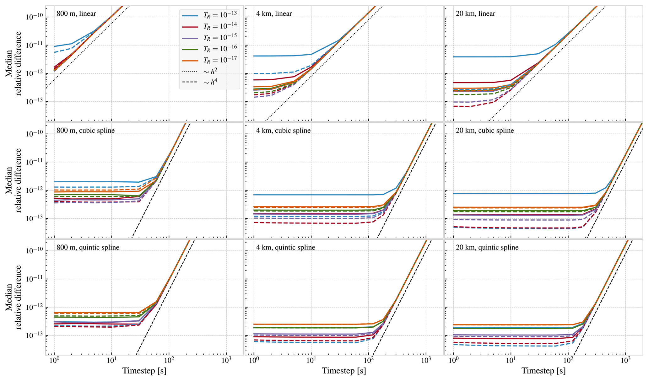
Figure A1 Median relative difference (Eqs. A1a and A1b) between the fourth-order Runge–Kutta solutions and the Dormand–Prince 8(7) solutions, as a function of the time step for the Runge–Kutta method, and shown for different tolerances for the Dormand–Prince method. The regular Dormand–Prince 8(7) is shown as continuous lines, and the special-purpose variant is shown as dashed lines.

For shorter time steps, we observe that the relative difference, Δ(h,T_R), flattens out and becomes constant. The interpretation of this, in light of Eq. (A1b), is that for the shorter time steps, Δ(h,T_R) is dominated by the error in the variable-step reference solution, thus appearing to be constant with the time step h. Based on this reasoning, we conclude that the most accurate variable-step solutions are obtained with the special-purpose integrator, with a tolerance of 10⁻¹³, 10⁻¹⁴, or 10⁻¹⁵, depending on the dataset and the order of interpolation.

Next, we do the opposite comparison, i.e. we use the fourth-order Runge–Kutta solutions as reference, keep the time step fixed and look at the relative difference, Δ(h,T_R), as a function of tolerance. The results are shown in Fig. A2. Starting from the high tolerances, we observe that the relative difference first goes down as the tolerance is reduced. Then, in all cases except the linearly interpolated 800 m dataset, the smallest estimated differences thereafter go up as the tolerance is reduced further. The reason is that the error in the variable-step solutions goes down until at some point the accumulated roundoff errors begin to dominate, and the error increases as the reduced tolerance leads to an increasing number of steps.

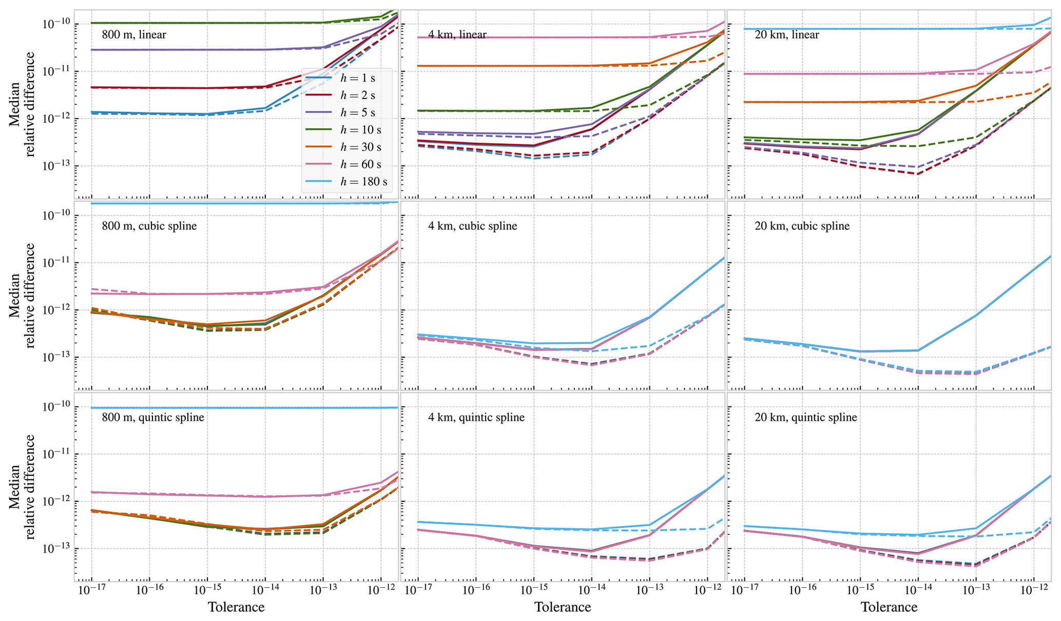
Figure A2 Median relative difference (Eqs. A1a and A1b) between the Dormand–Prince 8(7) solutions and the fourth-order Runge–Kutta solutions, as a function of the tolerance for the Dormand–Prince method, and shown for different time steps for the Runge–Kutta method. The regular Dormand–Prince 8(7) is shown as continuous lines, and the special-purpose variant is shown as dashed lines.

From Figs. A1 and A2 together, we conclude that the fourth-order Runge–Kutta solutions for short time steps are the most accurate solutions. As we can see from Eq. A1b, we are essentially considering the absolute value of the difference in the error of the fixed-step solution, and the error in the variable-step solution. Since Δ(h,T_R) (Fig. A1) appears to be constant with time step (for the shortest time steps), we conclude that Δ(h,T_R) is dominated by the (relatively) large constant error in the variable-step solution, obscuring the small changes with time step in the error in the fixed-step solution.

In order to further investigate the relative accuracy of the fourth-order Runge–Kutta solutions, we consider the change in the solution between two different values of the time step. First, we list all the time steps in Table A1, such that h₀=1 s, h₁=2 s, h₂=5 s, h₃=10 s, etc. Then we consider the quantity

$$\begin{array}{}\text{(A2a)}& {\displaystyle }\begin{array}{rl}& {\mathrm{\Delta }}_{\mathrm{RK}\mathrm{4}}(h_i,h_{i+\mathrm{1}}),\\ & ={\displaystyle \frac{\left|{\mathit{x}}_N\left(h_{i+\mathrm{1}}\right)-{\mathit{x}}_N\left(h_i\right)\right|}{\left|{\mathit{x}}_N\left(h_i\right)\right|}}\end{array}\text{(A2b)}& {\displaystyle }={\displaystyle \frac{\left|\left({\mathit{x}}_N\right(h_{i+\mathrm{1}})-\mathit{x}(t_N\left)\right)-\left({\mathit{x}}_N\right(h_i)-\mathit{x}(t_N\left)\right)\right|}{\left|{\mathit{x}}_N\left(h_i\right)\right|}}.\end{array}$$

As h_i and h_i+1 become smaller, we expect ${\mathrm{\Delta }}_{\mathrm{RK}\mathrm{4}}(h_i,h_{i+\mathrm{1}})$ to become smaller as well. Since the global error of a fourth-order Runge–Kutta method (for sufficiently smooth right-hand sides) is 𝒪(h⁴), we see from Eq. (A2b) that

$$\begin{array}{}\text{(A3)}& {\mathrm{\Delta }}_{\mathrm{RK}\mathrm{4}}\left(h_i,h_{i+\mathrm{1}}\right)\sim \left(\mathcal{O}\left(h_{i+\mathrm{1}}^{\mathrm{4}}\right)-\mathcal{O}\left(h_i^{\mathrm{4}}\right)\right).\end{array}$$

In Fig. A3, we plot ${\mathrm{\Delta }}_{\mathrm{RK}\mathrm{4}}(h_i,h_{i+\mathrm{1}})$, as a function of h_i. For the linearly interpolated datasets, we observe that ${\mathrm{\Delta }}_{\mathrm{RK}\mathrm{4}}(h_i,h_{i+\mathrm{1}})$ decreases proportionally to h², since the linearly interpolated right-hand sides are not sufficiently smooth to yield fourth-order convergence, and does not flatten out for small time steps. Hence, we conclude that the solutions obtained with time step h=1 s are the most accurate in this case.

Figure A3 Median relative difference (Eqs. A2a and A2b) between two fourth-order Runge–Kutta solutions, obtained with different time steps h_i and h_i+1, using the list of time steps in Table A1.

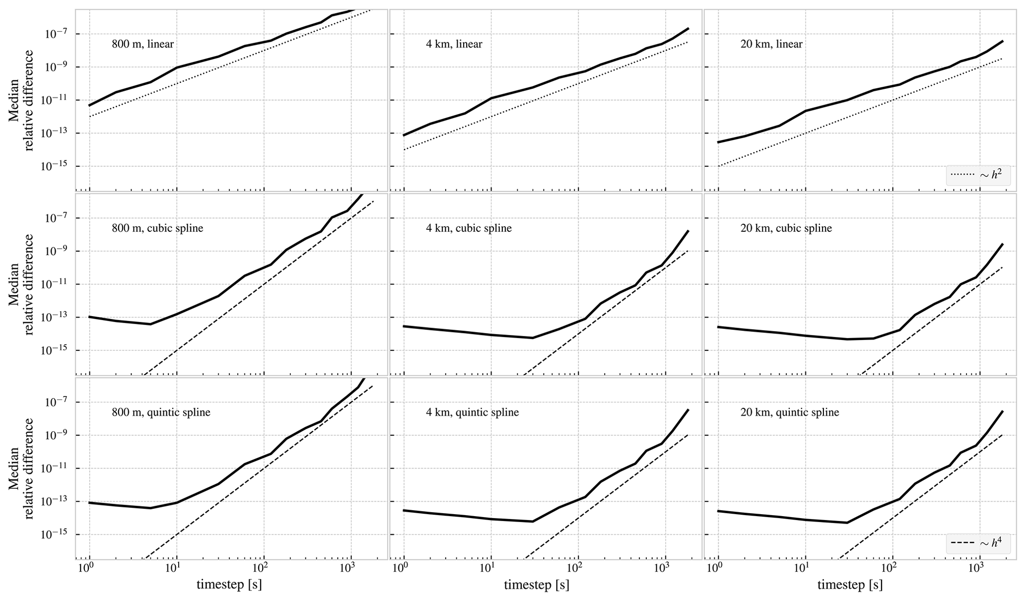
With cubic and quintic interpolation, we see that ${\mathrm{\Delta }}_{\mathrm{RK}\mathrm{4}}(h_i,h_{i+\mathrm{1}})$ goes down approximately as h⁴, and eventually flattens out and increases a little for the shortest time steps. As discussed previously, we interpret this to mean that the accumulated roundoff errors begin to dominate. We find that the smallest difference is obtained with different time steps for the different datasets. For example, for the 800 m resolution dataset, a time step h=5 s appears to be the most accurate, while for the 20 km dataset, a time step of 30 s appear to give better accuracy.

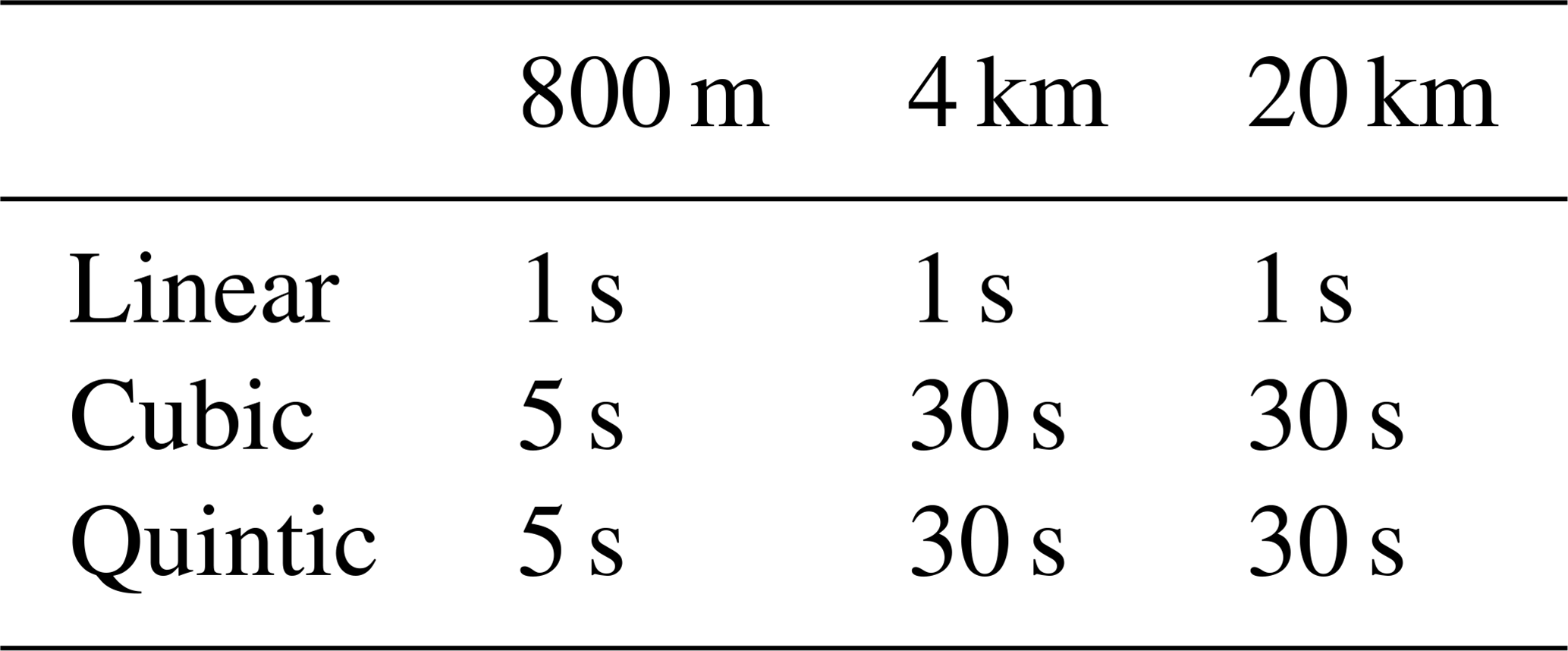
Based on the analysis described above, we have decided to use the fourth-order Runge–Kutta method to obtain the reference solutions used for the analysis in Sect. 5. For each dataset and order of interpolation, the reference time step is chosen based on Fig. A3, and the results are shown in Table A2.

Table A2 Time step used with the fourth-order Runge–Kutta method to obtain the reference solutions used in Sect. 5 for each order of interpolation and each dataset.

As a final remark, we mention that it may seem surprising that we are able to obtain higher accuracy with the fourth-order Runge–Kutta method than with the Dormand–Prince 8(7) method. Three things are worth pointing out in this context. First, the time steps considered here (see Table A1) all evenly divide the 1 h step of the data, which means that a fixed-step method will always stop and restart the integration at the discontinuities in the time-direction (see discussion in Sect. 3.1). Second, for the Dormand–Prince 8(7) method to work optimally, the right-hand side of the ODE should strictly have continuous partial derivatives up to order 8, which would require spline interpolation of degree 9. Finally, variable-step methods are generally preferred for their efficiency, not purely for their accuracy. As an example, consider the fifth-degree interpolated 800 m dataset. In this case, the presumed most accurate fixed-step solution, with h=5 s used 207 360 evaluations of the right-hand side, while the most accurate Dormand–Prince 8(7) solution, with a tolerance of 10⁻¹⁴, used 5805 evaluations (including 17 % rejected steps).

Appendix B: Additional work–precision diagrams

This appendix contains two additional figures to supplement the work–precision diagram shown in Fig. 5. See Sect. 5 for further details. First, in Fig. B1, we show the same data as in Fig. 5, i.e. the median global error over 10 000 trajectories, but with the addition of shaded areas that indicate the range covering 90 % of the errors.

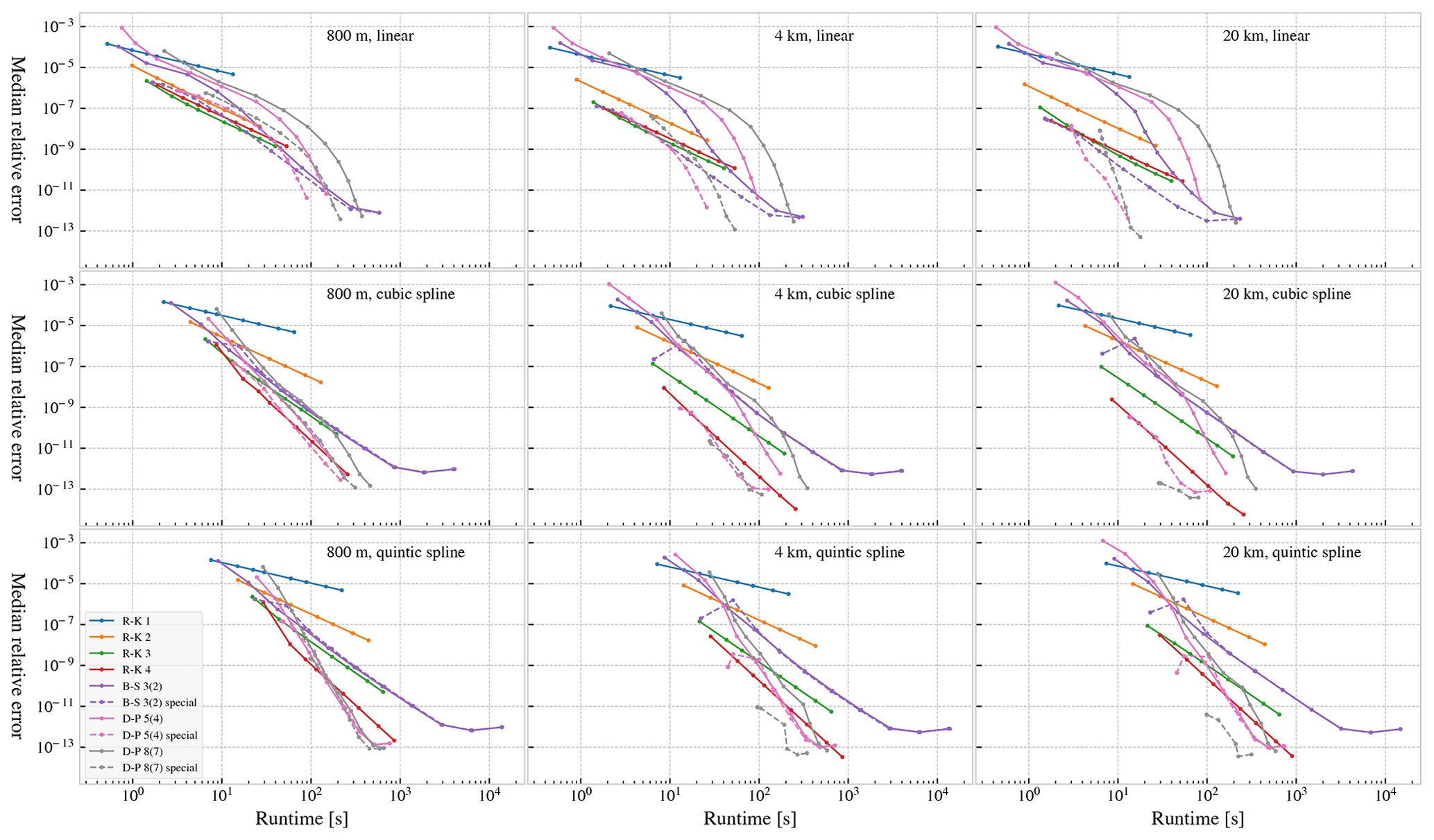
Second, Fig. B2 shows the median global error as a function of simulation runtime. The timings were obtained on a desktop workstation with an Intel Xeon 3.3 GHz CPU, running xubuntu 18.04. The code runs on a single core only. As discussed in Sect. 5, the number of evaluations of the right-hand side of the ODE is a more objective measure of work, as the runtime is susceptible to some random variation (in particular for the shortest simulations) due to other processes running on the machine, etc. However, we include the run times here as an illustration, as it is practically relevant information.

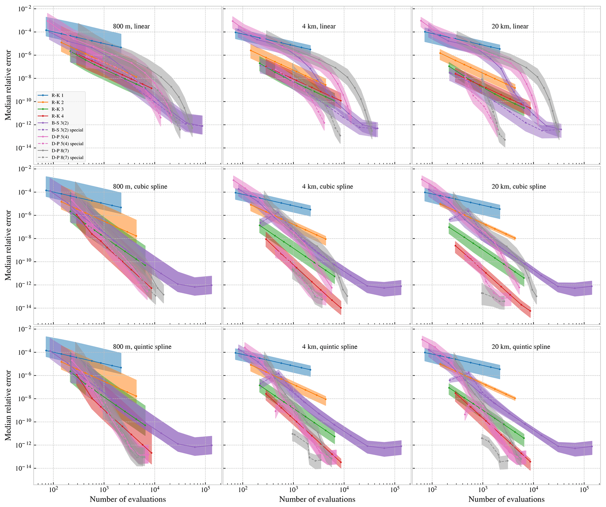
Figure B1 Same as Fig. 5, showing the median relative error taken over all 10 000 trajectories. Additionally, the shaded areas show the range where 90 % of the errors fall.

Figure B2 Same as Fig. 5, showing the median relative error, taken over all 10 000 trajectories, except that the median error is shown as a function of simulation runtime, rather than the number of evaluations of the right-hand side of the ODE.