PMIF v1.0: assessing the potential of satellite observations to constrain CO₂ emissions from large cities and point sources over the globe using synthetic data

This study assesses the potential of satellite imagery of vertically integrated columns of dry-air mole fractions of CO₂ (XCO₂) to constrain the emissions from cities and power plants (called emission clumps) over the whole globe during 1 year. The imagery is simulated for one imager of the Copernicus mission on Anthropogenic Carbon Dioxide Monitoring (CO2M) planned by the European Space Agency and the European Commission. The width of the swath of the CO2M instruments is about 300 km and the ground horizontal resolution is about 2 km resolution. A Plume Monitoring Inversion Framework (PMIF) is developed, relying on a Gaussian plume model to simulate the XCO₂ plumes of each emission clump and on a combination of overlapping assimilation windows to solve for the inversion problem. The inversion solves for the 3 h mean emissions (during 08:30–11:30 local time) before satellite overpasses and for the mean emissions during other hours of the day (over the aggregation between 00:00–08:30 and 11:30–00:00) for each clump and for the 366 d of the year. Our analysis focuses on the derivation of the uncertainty in the inversion estimates (the “posterior uncertainty”) of the clump emissions. A comparison of the results obtained with PMIF and those from a previous study using a complex 3-D Eulerian transport model for a single city (Paris) shows that the PMIF system provides the correct order of magnitude for the uncertainty reduction of emission estimates (i.e., the relative difference between the prior and posterior uncertainties). Beyond the one city or few large cities studied by previous studies, our results provide, for the first time, the global statistics of the uncertainty reduction of emissions for the full range of global clumps (differing in emission rate and spread, and distance from other major clumps) and meteorological conditions. We show that only the clumps with an annual emission budget higher than 2 MtC yr⁻¹ can potentially have their emissions between 08:30 and 11:30 constrained with a posterior uncertainty smaller than 20 % for more than 10 times within 1 year (ignoring the potential to cross or extrapolate information between 08:30–11:30 time windows on different days). The PMIF inversion results are also aggregated in time to investigate the potential of CO2M observations to constrain daily and annual emissions, relying on the extrapolation of information obtained for 08:30–11:30 time windows during days when clouds and aerosols do not mask the plumes, based on various assumptions regarding the temporal auto-correlations of the uncertainties in the emission estimates that are used as a prior knowledge in the Bayesian framework of PMIF. We show that the posterior uncertainties of daily and annual emissions are highly dependent on these temporal auto-correlations, stressing the need for systematic assessment of the sources of uncertainty in the spatiotemporally resolved emission inventories used as prior estimates in the inversions. We highlight the difficulty in constraining the total budget of CO₂ emissions from all the cities and power plants within a country or over the globe with satellite XCO₂ measurements only, and calls for integrated inversion systems that exploit multiple types of measurements.

1 Introduction

Cities, thermal power plants and industrial factories cover a very small fraction of the land surface but are emitting a large amount of CO₂. Many cities and regions are taking actions to reduce their greenhouse gas emissions. However, there are large uncertainties in the estimate of emissions from these CO₂ hotspots (Gately and Hutyra, 2017; Gurney et al., 2016). In addition, emissions at high temporal resolution (e.g., daily and hourly) depend on socio-economic activity and climate fluctuations and thus have large variability. The large uncertainties and fluctuations of emissions at local scale have raised a growing political and scientific interest for an accurate and continuous monitoring of these local CO₂ emissions based on atmospheric measurements (Duren and Miller, 2012).

Measurements of CO₂ mole fractions from in situ surface networks, aircraft campaigns and mobile platforms around cities (Bréon et al., 2015; Lauvaux et al., 2016; Staufer et al., 2016) have been used to characterize the CO₂ signals downwind of large cities and to quantify the underlying emissions based on an atmospheric inversion approach. However, such urban networks are deployed for a few cities only. Alternatively, vertically integrated columns of dry-air mole fractions of CO₂ (XCO₂) from satellites offer the opportunity to sample the atmosphere with global coverage. Kort et al. (2012) and Janardanan (2016) found that significant XCO₂ enhancements could be detected over some megacities using Greenhouse Gases Observing Satellite (GOSAT) XCO₂ observations. Schwandner et al. (2017) also found XCO₂ enhancements of 4.4 to 6.1 ppm in the Los Angeles urban CO₂ dome using observations from the Orbiting Carbon Observatory-2 (OCO-2). Nassar et al. (2017) used the XCO₂ observations from OCO-2 to quantify CO₂ emissions from several medium- to large-sized coal power plants. However, the design of GOSAT and OCO-2 observations with sparse sampling was mainly focused on the monitoring of CO₂ natural fluxes. Recent studies show a limited amount of clear detections of transects of XCO₂ plumes from cities or plants in OCO-2 observations (Zheng et al., 2020) so that GOSAT and OCO-2 data keep on being hardly used to estimate CO₂ city emissions. The potential for reducing uncertainties in CO₂ emissions at the scale of point sources (Bovensmann et al., 2010), cities (Broquet et al., 2018; Pillai et al., 2016) and agglomerations of several cities (O'Brien et al., 2016) should dramatically change with the planned satellite missions with imaging capabilities. These studies consistently showed that imaging capability with a wide swath (typically on the order of 200–300 km), a high resolution (<2–3 km horizontal resolution) and a high single sounding precision (<2 ppm) are required for satellite XCO₂ measurements for the monitoring of CO₂ emissions from large point sources and cities. Several satellite XCO₂ imagery concepts have been proposed: (i) the OCO-3 NASA (National Aeronautics and Space Administration) mission which has been installed on the International Space Station (ISS) in May 2019; (ii) the CarbonSat mission which was a candidate for the European Space Agency's (ESA's) Earth Explorer 8 opportunity (Bovensmann et al., 2015) but was not selected; (iii) the “city-mode” of the MicroCarb mission of the Centre National d'Etudes Spatiales (CNES), which should be launched in 2021 (Bertaux et al., 2019); (iv) the GeoCARB geostationary mission which was selected as the Earth Venture Mission-2 by NASA; and (v) the Copernicus Anthropogenic Carbon Dioxide Monitoring (CO2M) mission consisting of a constellation of CO₂ imagers that is currently studied by the ESA on behalf of the European Commission in the context of the European Union Copernicus programme. This CO2M satellite constellation is a crucial element that will contribute to the operational anthropogenic CO₂ monitoring and verification support capacity currently under development by the European Commission with support from the ESA, European Organisation for the Exploitation of Meteorological Satellites (EUMETSAT) and the European Centre for Medium-Range Weather Forecasts (ECMWF) (Ciais et al., 2015; Pinty et al., 2017, 2019).

The main approach currently investigated for the estimate of CO₂ emissions from satellite XCO₂ images consists of identifying the XCO₂ plumes downwind of the main CO₂ emission sources. The size of the plumes and the magnitude of XCO₂ enhancements in these plumes are tightly linked to the emissions. Wang et al. (2019) developed an algorithm to extract, from gridded emission maps, a conservative set of area (cities) and point sources (power plants) with intense emissions around the globe which can generate coherent XCO₂ plumes that may be observed from space, given the precision of current satellite observations. This set was conservative because it is inferred for idealized meteorological condition without wind. These emitting sources were called “emission clumps”. Wang et al. (2019) identified 11 314 individual clumps which contribute 72 % of the global fossil fuel CO₂ emissions from the ODIAC (Open-source Data Inventory for Anthropogenic CO₂ version 2017; Oda et al., 2018) 1 km resolution inventory.

Broquet et al. (2018) showed that the part of the XCO₂ plumes exploited by the atmospheric inversion in satellite images corresponds to a few hours of the clump emissions before the satellite overpass. The XCO₂ signature of the earlier clump emissions is too diluted to be filtered from the measurement errors and the signature of other CO₂ sources and sinks. Further, emissions from a given clump vary in time during the day, for instance due to the variations of traffic in cities (Yang et al., 2019), from day to day and between seasons, with more emissions associated with heating in winter over cold regions (Bréon et al., 2017). Therefore, the estimate of annual budgets of the clump emissions based on satellite observation during daytime (generally for a fixed local time since most of the missions use heliosynchronous orbits) and for low cloud coverage is a challenge and cannot rely on the direct information from the satellite imagery. It relies on the extrapolation of information from the time windows for which the emissions are well constrained. Such an extrapolation is based on the correlation of the uncertainty in emissions in time, and more precisely, in the atmospheric inversion framework, on the temporal auto-correlations of the uncertainty in the inventories used as a prior knowledge by the Bayesian framework of the inversion (see Sect. 2.6).

Previous studies on the potential of the satellite XCO₂ imagery to constrain the emissions from clumps were limited to a single target or a few large targets, such as power plants in Bovensmann et al. (2010), Berlin in Pillai et al. (2016) and in Kuhlmann et al. (2019), and Paris in Broquet et al. (2018). However, much of the global CO₂ emissions occur in smaller cities and plants. The potential and design of satellite missions dedicated to the monitoring of the CO₂ emissions like CO2M needs to be assessed for a much more representative range of sources over the whole globe. The inversion framework used by Pillai et al. (2016) and Broquet et al. (2018) were based on full 3-D Eulerian atmospheric transport models at high spatial resolution (on the order of 2 km). Such inversions are much too expensive in terms of computation cost to be applied in a systematic way to the full set of clumps across the globe.

Therefore, in this study, we develop a Plume Monitoring Inversion Framework (PMIF) and conduct a set of observing system simulation experiments (OSSEs) to assess, for the first time, the performance of a satellite instrument to monitor the emissions of all the clumps across the globe and over a whole year. The imager studied has the foreseen characteristics of the individual satellites of the forthcoming CO2M mission. It would be a high-resolution spectrometer, with 2 km×2 km resolution pixels and a swath of 300 km, and it would be placed on a Sun-synchronous orbit ensuring global coverage in 4 d. The PMIF inversion system relies on the list of clumps extracted by Wang et al. (2019) from the ODIAC inventory, on the Gaussian plume model to simulate the XCO₂ plumes generated by the emissions from these clumps, on an analytical inverse modeling framework, and on a combination of overlapping assimilation windows to solve for the inversion problem over the globe and a full year. It also addresses the question of temporal extrapolation that is needed to generate estimates of annual emissions from the information of a limited number of time windows for which emissions are well constrained by the direct satellite images, by accounting for the temporal auto-correlation of the prior uncertainties. The performance is assessed in terms of the uncertainties in the emissions (Sect. 2.1) at different scales. The PMIF uses a Gaussian plume model at the local scale to ensure that the computation cost is affordable. Such a model can often hardly fit with actual plumes over the distances considered in this study (due to variations in the wind field, topography, vertical mixing etc. over such distances) but is shown, when driven with suitable parameters, to provide a satisfactory simulation of the plume extent and amplitudes, which appear to be the main drivers of the targeted computations of uncertainties in the emissions in our OSSE framework (as shown in Sect. 3.1). In PMIF, we also ignore the impact of some sources of uncertainties on the inversion of emissions, including systematic errors in the XCO₂ retrievals, the impact of uncertainties in diffuse anthropogenic emissions outside clumps and in non-fossil CO₂ fluxes (within and outside clumps), and in the spatial and temporal variations of emissions within the clump and in the short time windows that the inversion aims to solve. These impacts are discussed in detail afterwards.

This PMIF system provides an indication of the satellite system capabilities for the full range of cities and power plants varying in topography, emission budget and spread, proximity to other major sources, and for a large range of meteorological conditions. It complements other systems that focus on specific regions with more complex (but area-limited) models and consideration of diffuse sources and natural fluxes, allowing for extrapolating and up-scaling results of those more complex systems to get a more systematic understanding of their implications for the monitoring of CO₂ emissions from all detectible clumps over the globe.

The PMIF system and the OSSEs analyzed in this first study are described in Sect. 2. The results obtained with the PMIF for the city of Paris are compared with those of Broquet et al. (2018) in Sect. 3.1. The uncertainty in the retrieved emissions of individual clumps with one imaging satellite for 3 h time windows, for daily emissions and for annual emissions is assessed in Sect. 3.2–3.4. Section 4 discusses the drivers of the spatial variations of the uncertainty in the retrieved emissions, the limitations of PMIF and the implications for a future operational observing system.

2 Methodology

2.1 Plume Monitoring Inversion Framework

The theoretical framework of the inversion system developed in this study is the same as the traditional atmospheric inversions. The inversion derives a statistical estimate for a set of control variables x in a model $\mathit{x}\to \mathit{y}=\mathbf{M}\mathit{x}$ that simulates the satellite XCO₂ measurements y^o. The model M linking x and y is a combination of flux and atmospheric transport models (detailed in Sect. 2.4) and is called observation operator hereafter. As explained below, we do not have a constant term added to Mx in the observation operator of the PMIF that would gather the atmospheric CO₂ signature of the fluxes not controlled by the inversion (like non-fossil fluxes and the background XCO₂ field) since the uncertainty in such fluxes is ignored. The inversion follows a Bayesian statistical framework, updating the statistical prior estimate of x based on the statistical information from the assimilation of XCO₂ measurements y into the observation operator. The distributions of the prior estimate and of the misfits between the actual observations y^o and simulated ones due to errors in the observations and in the observation operator (called the “observation errors”) are assumed to be unbiased and to have the Gaussian forms N(x^b,B) and N(0,R), where B and R are the prior and observation error covariance matrices. The statistical distribution of the posterior estimate of x, given the observation operator, x^b and y^o, also follows a Gaussian distribution N(x^a,A), with x^a being the mean and A being the error covariance matrix characterizing the posterior uncertainty. The problem is solved by deriving the following:

$$\begin{array}{}\text{(1)}& {\displaystyle }& {\displaystyle }\mathbf{A}={\left({\mathbf{B}}^{-\mathrm{1}}+{\mathbf{M}}^{\mathrm{T}}{\mathbf{R}}^{-\mathrm{1}}\mathbf{M}\right)}^{-\mathrm{1}},\text{(2)}& {\displaystyle }& {\displaystyle }{\mathit{x}}^{\mathrm{a}}={\mathit{x}}^{\mathrm{b}}+{\mathbf{AM}}^{\mathrm{T}}{\mathbf{R}}^{-\mathrm{1}}\left({\mathit{y}}^{\mathrm{o}}-\mathbf{M}{\mathit{x}}^{\mathrm{b}}-{\mathit{y}}^{\mathrm{fixed}}\right),\end{array}$$

where ^T and ⁻¹ denote the transpose and inverse of a given matrix.

Equation (1) shows that A only depends on prior and observation error covariance matrices, on the observation operator, and implicitly on the structure of the observation vector (i.e., on the time, location and representation of the observations in M), while Eq. (2) shows that x^a also depends on the actual value of x^b and y^o. PMIF is an analytical inversion system that solves for Eq. (1) or for an approximation of this equation (when accounting for temporal correlations in B) by building the different matrices involved in this equation.

We characterize B, R and A by the corresponding standard deviations (σ) of uncertainty in individual control parameters or aggregations of control parameters and by the temporal auto-correlations of the uncertainties (Sect. 2.6). In the following, the “uncertainty reduction” for a given control variable or for an aggregation of control variables (like emission budgets over larger timescales than that of the control vector) refers to the relative difference between its prior and posterior uncertainty: $\mathrm{1}-{\mathit{\sigma }}_{\mathrm{a}}/{\mathit{\sigma }}_{\mathrm{b}}$.

We use a Gaussian plume model (Sect. 2.4) to simulate the atmospheric transport at a spatial resolution consistent with that of the XCO₂ measurements from the planned CO₂ imager and with the highly heterogeneous distribution of emissions. Compared with complex 3-D atmospheric transport models, Gaussian plume models have a very low computational cost, making the global assessment of posterior uncertainty and uncertainty reduction at the scale of emission clumps from the assimilation of high-resolution data feasible. However, since a Gaussian plume model provides a highly simplified approximation of the atmospheric transport from emission clumps, we need to verify that its use in the PMIF yields estimates of the uncertainties in the inverted emissions that are consistent with those that would be based on more complex models. Therefore, we first compare the results for Paris from PMIF against those acquired based on a 3-D Eulerian atmospheric transport model by Broquet et al. (2018), the latter also accounting for uncertainties in diffuse CO₂ fluxes. On the one hand, the signals from these diffuse and natural CO₂ fluxes cannot be modeled effectively by a Gaussian plume model. On the other hand, the diffuse and natural CO₂ fluxes in Paris were shown to have only a weak impact on the inversion of whole-city CO₂ emissions (Staufer et al., 2016). For this comparison, we use the same simulation of the XCO₂ sampling by CarbonSat (Sect. 2.2) and a similar control vector to Broquet et al. (2018). The corresponding inversion with the PMIF is called PMIF-Paris hereafter. Then we apply the system to all the emission clumps over the globe and over 1 year using a different control vector and a simulation of the XCO₂ sampling by a single CO2M satellite (Sect. 2.2). The inversions for all emission clumps over the globe are called PMIF-Globe. In PMIF-Globe, we first investigate the potential of satellite observations in constraining emissions from individual time windows (ExpNoCor in Sect. 2.6). Then we assess the ability of satellite observations to constrain emissions at annual scale by accounting for the temporal auto-correlation of the prior uncertainties (other experiments in Sect. 2.6). Tables 1 and 2 summarize the different options for the configuration of the system and of the OSSEs. One distinction between PMIF-Paris and PMIF-Globe is that PMIF-Paris relates XCO₂ signals with the mean emissions 6 h before overpasses, while it is assumed that in PMIF-Globe that the XCO₂ signals only provide effective constraints on 3 h mean emissions before individual overpasses. The 6 h period corresponds to the period of emissions from Paris whose signature in the XCO₂ field can still be detected by the satellite despite the atmospheric diffusion (Broquet et al., 2018). While Broquet et al. (2018) indicated that the period of “detectable” emissions from a large megacity like Paris could last up to 6 h, most of the clumps across the globe have smaller emission rates than Paris or are located in more complex environment close to other major emission areas where XCO₂ signals can be attributed to multiple sources, making the detection of the XCO₂ signature of emissions a few hours before the satellite overpass even more difficult. For the PMIF-Globe experiments, we thus conservatively assume that the XCO₂ signals can only provide effective constraints on 3 h mean emissions before individual overpasses in general.

Table 1 The configuration of the PMIF-Paris inversion.

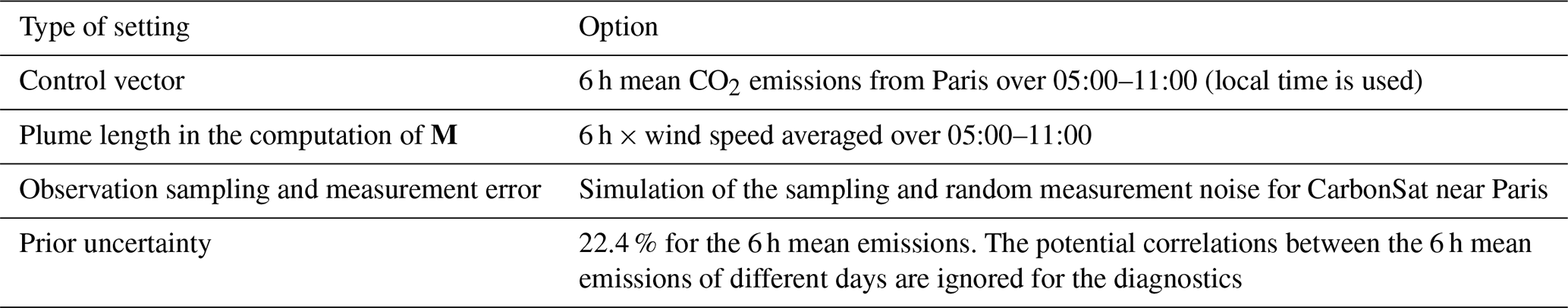
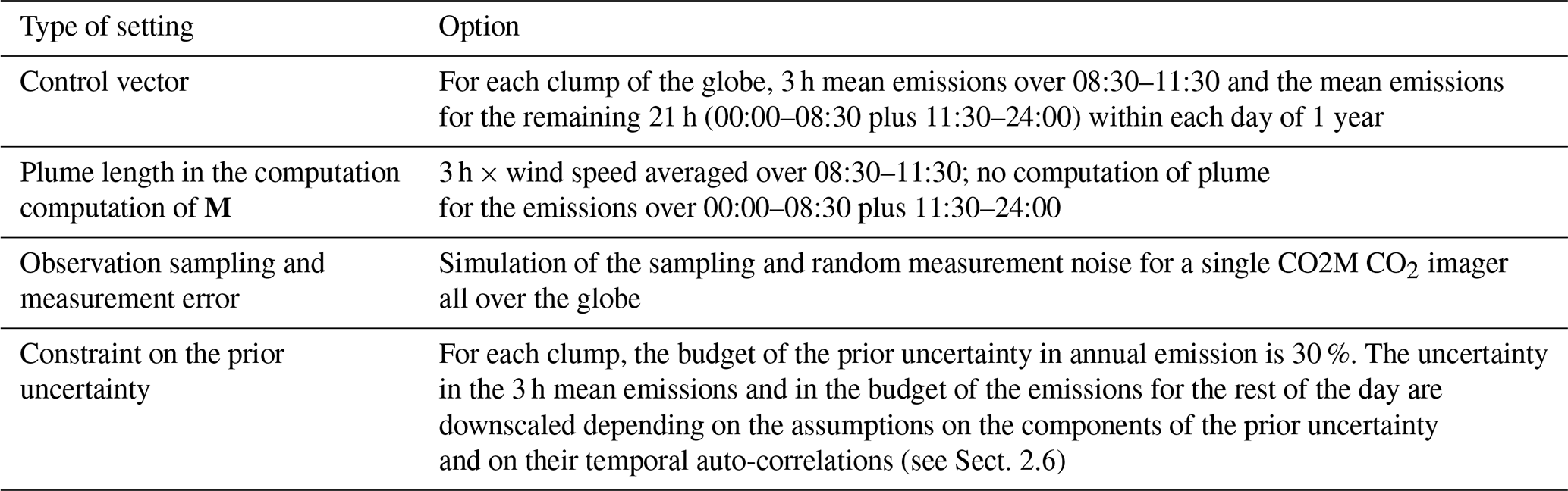
Table 2 The different options for the configuration of PMIF-Globe inversions.

2.2 Observation space

In this study, we consider the samplings from two different virtual CO₂ imagers.

The first sampling used in PMIF-Paris (Table 1 and Sect. 2.7.1) is the simulation of the sampling for CarbonSat by Buchwitz et al. (2013) exactly as in Broquet et al. (2018). XCO₂ is sampled by a 240 km swath instrument with 2 km spatial resolution. Given the presence of cloud and aerosol and their impacts on the precision of XCO₂ retrievals, only “good” XCO₂ observations, for which the sum of the retrieved aerosol optical depth (AOD) at near-infrared (NIR) wavelength and atmosphere cirrus optical depth (COD) is less than 0.3, are used in the inversions. The preferable condition, $\text{AOD(NIR)}+\text{COD}<\mathrm{0.3}$, for a good XCO₂ observation is referred to as “clear sky” hereafter. The CarbonSat sampling was simulated over the whole globe and for a full year by Buchwitz et al. (2013), but it is used here for the inversion of the emission of Paris only. Thus, only the passes with at least one good XCO₂ measurement in the 100 km radius circle centered on Paris are used, as in Broquet et al. (2018).

The second sampling is global and is used for all the other experiments of PMIF-Globe (Table 2 and Sect. 2.7.2). It corresponds to that of a single CO2M satellite with a 300 km swath and 2 km spatial resolution. CO2M is similar to CarbonSat for sampling but has a larger swath and better precision (Sect. 2.5). The simulation is based on the method and model described by Buchwitz et al. (2013) but uses different values for the parameters in the model.

2.3 Control vector

In the PMIF-Paris inversion, the satellite observations are sampled at 11:00 local time, in line with the experiments from Broquet et al. (2018). The inversion solves for the mean emissions for the 6 h before 11:00 local time. Broquet et al. (2018) solved for the hourly emissions during this 6 h period but PMIF can only solve for the mean emissions during the 6 h period due to the fact that the Gaussian plume model cannot be used to compute the signatures in the XCO₂ field of individual hourly emissions during that period. The control vector in PMIF-Paris thus consists of a set of scaling factors for the mean emission between 05:00 and 11:00 for all individual overpasses near Paris (Sect. 2.7.1). The prior and posterior scaling factors are used to rescale the 1 h and ∼1 km resolution emission fields from an emission map and its temporal profile which are parts of the observation operator (Sect. 2.4).

In the PMIF-Globe inversion, the satellite observations are sampled at a local time of approximately 11:30 over all the clumps. The inversion solves for a scaling factor for 3 h mean emissions between 08:30 and 11:30 and a scaling factor for the emissions during of the rest of the day (00:00–08:30 plus 11:30–24:00) for each day over 1 year and for all the clumps over the globe:

$$\begin{array}{}\text{(3)}& \begin{array}{rl}& \mathit{x}=[{\mathit{\lambda }}_{\mathrm{clump}\mathrm{1}}^{\mathrm{day}\mathrm{1},\mathrm{morning}},{\mathit{\lambda }}_{\mathrm{clump}\mathrm{1}}^{\mathrm{day}\mathrm{1},\mathrm{rest}},{\mathit{\lambda }}_{\mathrm{clump}\mathrm{1}}^{\mathrm{day}\mathrm{2},\mathrm{morning}},{\mathit{\lambda }}_{\mathrm{clump}\mathrm{1}}^{\mathrm{day}\mathrm{2},\mathrm{rest}},\\ & \mathrm{\dots },{\mathit{\lambda }}_{\mathrm{clump}\mathrm{1}}^{\mathrm{day}\mathrm{366},\mathrm{morning}},{\mathit{\lambda }}_{\mathrm{clump}\mathrm{1}}^{\mathrm{day}\mathrm{366},\mathrm{rest}},{\mathit{\lambda }}_{\mathrm{clump}\mathrm{2}}^{\mathrm{day}\mathrm{1},\mathrm{morning}},\\ & {\mathit{\lambda }}_{\mathrm{clump}\mathrm{2}}^{\mathrm{day}\mathrm{1},\mathrm{rest}},\mathrm{\dots },{\mathit{\lambda }}_{\mathrm{clumpN}}^{\mathrm{day}\mathrm{366},\mathrm{morning}},{\mathit{\lambda }}_{\mathrm{clumpN}}^{\mathrm{day}\mathrm{366},\mathrm{rest}}].\end{array}\end{array}$$

In both types of experiments, we do not include the diffuse emissions outside the selected clumps and the natural fluxes (more generally, any parameter of the “background concentrations”, Kuhlmann et al., 2019) in the control vector. The setup of the R matrix also ignores uncertainties in the background concentrations (Sect. 2.5). This is another divergence from the inversion configuration of Broquet et al. (2018), who accounted for such uncertainties.

2.4 Observation operator

The observation operator in PMIF (which is used in Eq. 1) is composed of two sub-operators. The first operator (M_inventory) describes the spatial distribution (within the clumps) and temporal variations of the emissions whose budgets are controlled by the inversion during 08:30–11:30 and during the remaining 21 h for each clump: $\mathit{x}\to \mathit{E}={\mathbf{M}}_{\mathrm{inventory}}\mathit{x}$. The spatial distribution of the emissions are based on estimates from ODIAC (Oda et al., 2018) for the year 2016. ODIAC provides the monthly mean emissions for 12 months through a year at a $\mathrm{0.0083}{}^{\circ }\times \mathrm{0.0083}{}^{\circ }$ (approximately 1 km×1 km) spatial resolution. The weekly and diurnal (at hourly resolution) profiles from the Temporal Improvements for Modeling Emissions by Scaling (TIMES) product (Nassar et al., 2013) are applied to the monthly emission maps of ODIAC to generate the hourly emission fields. The second operator (M_plume) simulates the plumes of XCO₂ enhancement above the background at and downwind of the emission clumps at 11:30: $\mathit{E}\to \mathit{y}={\mathbf{M}}_{\mathrm{plume}}\mathit{E}$. We assume that the plume of XCO₂ enhancement related to a given emitting pixel within a clump of the ODIAC map has a Gaussian shape and the plume from a clump is a sum of multiple Gaussian plumes from all the ODIAC pixels within that clump. For a given emitting pixel, the Gaussian plume model writes the following:

$$\begin{array}{}\text{(4)}& \mathit{y}\left(i,j\right)=\mathit{\alpha }{\displaystyle \frac{E}{\sqrt{\mathrm{2}\mathit{\pi }}{\mathit{\sigma }}_{j}u}}{e}^{-\frac{j^{\mathrm{2}}}{\mathrm{2}{\mathit{\sigma }}_j^{\mathrm{2}}}},\end{array}$$

where y is the XCO₂ enhancement (in ppm) downwind of the emitting pixel. The i direction is parallel to the wind direction, and the j direction is perpendicular to the wind direction. y depends on the mean emission rate during 08:30–11:30 at local time (E, in g s⁻¹), the wind speed (u, in m s⁻¹), the cross-wind distance (j) and the parameter σ_j (see below). The wind direction and speed is taken from the Cross-Calibrated Multi-Platform (CCMP) gridded surface wind fields for the year 2008 (Atlas et al., 2011). The CCMP product uses a variational analysis method (VAM) to combine the data from Version-7 RSS radiometer wind speeds, QuikSCAT and ASCAT scatterometer wind vectors, moored buoy wind data, and ERA-Interim model wind fields. The σ_j is a function of downwind distance i and atmospheric stability parameter ${\mathit{\sigma }}_j=\mathit{\beta }j/(\mathrm{1}+\mathit{\gamma }j{)}^{-\mathrm{1}/\mathrm{2}}$, where α is a coefficient that converts the computed XCO₂ enhancement in the unit of parts per million, and β and γ are coefficients depending on the atmospheric Pasquill stability category, which is a function of the wind speed and solar radiation (Turner, 1970). The values for β and γ can be found in Bowers et al. (1980). The original Gaussian plume model generates a stationary plume of an infinite length and width downwind of the emissions. Because we assume that the XCO₂ plumes sampled from a satellite overpass is only related to the emissions 3 h before, the Gaussian plume corresponding to each emitting pixel is cut off at the downwind distance equaling the wind speed multiplied by 3 h. The width of the plume is also cut off beyond 3 times the value of σ_j in the cross-wind direction. The observation operator is null for emission of the remaining 21 h (00:00–08:30 plus 11:30–24:00).

The size of the full theoretical control vector corresponds to 11 314 emission clumps times 2 time windows for each day times 366 d. The size of this full theoretical observation vector over the year is thus more than 30 000 000. Building matrices and applying Eq. (1) with such spaces is, in practice, not computationally affordable. Therefore, we divide the globe into 5400 spatial inversion windows (from 180^∘ W to 180^∘ E and from 90^∘ N to 60^∘ S), each inversion window covering an area of $\mathrm{10}{}^{\circ }\times \mathrm{10}{}^{\circ }$ and being extended on the four boundaries with margins of 500 km to ensure that the plumes from the clumps near the boundary of inversion windows are fully simulated and accounted for in the corresponding inversions. M_plume is constructed with a set of block matrices, each block representing a single spatial inversion window and a single day. When an emission clump and its plume are comprised within more than one inversion window on a single day, only the results obtained in the window that covers the full plume is used in M_plume.

2.5 Observation error

We evaluate the projection of the measurement noise of the satellite observation and ignore uncertainties in the observation operator. The measurement noise is derived from the simulations of random measurement errors from Buchwitz et al. (2013), and the impact of the systematic measurement errors is ignored. The random measurement errors are simulated as a function of geographic location (e.g., solar zenith angle, SZA), surface (e.g., albedo) and atmosphere characteristics (e.g., AOD). The random measurement error is 1.4 ppm for vegetation albedo and SZA 50^∘ in the CS sampling, and it is 0.7 ppm in the CO2M sampling, thus being 2 times smaller for the latter. The random measurement errors are uncorrelated from one XCO₂ data to the other, and the R matrix is thus a diagonal matrix as generally done in atmospheric inversion.

2.6 Specification of the prior uncertainties and of their temporal auto-correlations

Two configurations for the prior uncertainty are used in the OSSEs (Sect. 2.7). In the PMIF-Paris inversion, the prior uncertainty is 22.4 % for the each of the scaling factors for 6 h mean emission, the choice of this value being consistent with the configuration used by Broquet et al. (2018).

In the PMIF-Globe inversions, the prior uncertainty is downscaled from its estimate for the annual budget of emissions of each clump. A prior uncertainty in annual emission of 30 % is assumed for all clumps. This value is chosen to be of the same order of magnitude as the typical difference between emission inventories for a single point source and city. For example, Gurney et al. (2016) found that one-fifth of the power plants had monthly emission differences larger than 13 % between the estimates by two different US agencies. Gurney et al. (2019) compared the emission maps from ODIAC and Hestia for four US cities and found the whole-city differences are between −1.5 % and +20.8 %. Gately and Hutyra (2017) compared the inventories reported by local authorities and bottom-up fossil fuel CO₂ emission maps for 11 US cities and found the differences range from 33 % to 78 %. Then, the downscaling of the uncertainty in annual emissions into uncertainties at the sub-daily scale of the control variables (i.e., 3 h mean emission over 08:30–11:30 and 21 h mean emission during the rest of the day; Sect. 2.3) follows a decomposition of the total uncertainty into components with different temporal auto-correlations.

The hourly emissions in inventories are usually derived from the periodic typical temporal profiles to annual emissions (Andres et al., 2011; Nassar et al., 2013). There are large variations in actual emissions from hour to hour and from day to day, resulting in large differences between the emission estimates derived based on typical temporal profiles and actual emissions. These differences are sources of uncertainties in the emission inventories which are used in the inversion as prior information. However, there is no consensus regarding the uncertainty in emission inventories and their error structures (Gurney et al., 2019). We compare the typical temporal profiles of transport emissions and energy sector from the TIMES product with the TOMTOM traffic index (https://www.tomtom.com/en_gb/, last access: 20 September 2020, which provides indications of the level of variability in the traffic, though not of that of the CO₂ emissions themselves), respectively, and with the actual hourly CO₂ emissions from electricity production in France (https://www.services-rte.com/en/home.html, last access: 17 July 2017). Although these comparisons are only made for two sectors, the results already show that it is challenging to describe the temporal auto-correlations of the uncertainty in emissions with simple exponentially decaying functions (Figs. S1 and S2 in the Supplement) like what is usually done in traditional atmospheric inversions (Chevallier et al., 2010; Kountouris et al., 2015). We thus make several assumptions regarding the decomposition of the prior uncertainty into components with different modes of auto-correlation.

In some scenarios, we consider an “annual component” that is fully correlated in time over 1 year. We also consider “uncorrelated” components whose temporal auto-correlations are null and “sub-annual” components whose temporal auto-correlations follow the exponential decaying model with a correlation length smaller than 1 year. Specifically, we assume that the correlation between two instants of the sub-annual component at hourly scale is described by the following:

$$\begin{array}{}\text{(5)}& r=\exp \left(-\mathrm{\Delta }h/{\mathit{\tau }}_{\mathrm{1}}\right)\times \exp \left(-\mathrm{\Delta }d/{\mathit{\tau }}_{\mathrm{2}}\right),\end{array}$$

where Δh is the time lag (in hours) between the two times of the day that are considered, and Δd is the time lag (in days) between the two dates that are considered. The parameters τ₁ and τ₂ follow the fit of the misfits between the TIMES profiles and the TOMTOM and electricity production indices to the exponential functions at the hourly scale and at the daily scale, respectively (Figs. S1 and S2). The temporal auto-correlations between the emissions during the aggregated time windows (08:30–11:30 and the remaining 21 h) are computed by re-aggregating the uncertainties at the hourly scale, accounting for temporal auto-correlation.

The detailed configuration of the different scenarios for the decomposition of the prior uncertainty are listed below:

• 1.

  Annual component and moderately correlated sub-annual component (AMS). This is composed of an annual component and a sub-annual component. The temporal auto-correlation of the sub-annual component follows Eq. (5) with τ₁=12 h and τ₂=7 d. The ratio of the uncertainty in the annual component to that in the sub-annual component for 3 h emissions is assumed to be 3:5. This leads to an annual uncertainty component ∼N(0, 29 %) and a sub-annual component ∼N(0, 49 %) for 3 h emissions and ∼N(0, 38 %) for 21 h emissions.

• 2.

  Annual component and strongly correlated sub-annual component (ASS). This is composed of an annual component and a sub-annual component. The temporal auto-correlation of the sub-annual component follows Eq. (5) with τ₁=2400 h, which approximately corresponds to having full correlations between hourly uncertainties within a single day, and τ₂=20 d. The ratio of the uncertainty in the annual component to that in the sub-annual component for 3 h emissions is assumed to be 3:5. This leads to an annual uncertainty component ∼N(0, 26 %) and a sub-annual component ∼N(0, 44 %) for 3 h emissions and ∼N(0, 44 %) for 21 h emissions.

• 3.

  Moderately correlated sub-annual component (MCS). This is composed of a sub-annual component. The temporal auto-correlation of the sub-annual component follows Eq. (5) with τ₁=12 h and τ₂=7 d. This leads to a sub-annual component ∼N(0, 198 %) for 3 h emissions and ∼N(0, 119 %) for 21 h emissions.

• 4.

  Strongly correlated sub-annual component (SCS). This is composed of a sub-annual component. The temporal auto-correlation of the sub-annual component follows Eq. (5) with τ₁=2400 h and τ₂=20 d. This leads to a sub-annual component ∼N(0, 93 %) for 3 h emissions and ∼N(0, 93 %) for 21 h emissions.

• 5.

  Sector-dependent correlated sub-annual component (SectCS). This is composed of a sub-annual component for each emission sector. It is assumed that the relative uncertainty for different sectors are the same. The temporal auto-correlation of the sub-annual components for all sectors follow the same formulation as in Eq. (5), but with different τ₁ and τ₂. For the emissions in the industry sector, τ₁=2400 h and τ₂=180 d; for the emissions in the transport sector, τ₁=12 h and τ₂=7 d; for the emissions from energy sector, τ₁=24 h and τ₂=7 d; and for the emissions from other sectors, τ₁=24 h and τ₂=14 d. For each clump, the share of emissions from each sector are estimated according to EDGARv4.3.2 (https://edgar.jrc.ec.europa.eu/, last access: 25 July 2019). This leads to an uncertainty in 3 h emissions ranges between 40 % and 198 %, and in 21 h emissions ranges between 40 % and 154 %.

• 6.

  No temporal auto-correlation (NoCor). We assume that the uncertainties in 3 h emissions and 21 h emissions on all days are all random and uncorrelated from one time window to the other, or from one day to the other. The resulting sub-annual component follows the distribution ∼N(0, 1623 %) for 3 h emissions and ∼N(0, 614 %) for 21 h emissions.

The prior uncertainty in the 3 h mean emissions between 08:30 and 11:30 is close to or larger than 100 % in scenarios SCS and MCS, and it even reaches an abnormally huge value of 1623 % in NoCor. Andres et al. (2016) estimated the uncertainty in the widely used emission map CDIAC (Carbon Dioxide Information Analysis Center). They found that the average uncertainty in monthly emissions for one $\mathrm{1}{}^{\circ }\times \mathrm{1}{}^{\circ }$ grid cell is 120 % and further suspected that the uncertainties in hourly and daily emissions at urban scale could be even larger (from a few percent to 1000 %). But these large values challenge the assumption that the uncertainty in anthropogenic emissions is normally distributed (Gurney et al., 2019). In this study, we follow the traditional assumption used in atmospheric inversions that the prior uncertainty follows a Gaussian distribution, allowing the prior uncertainty to exceed 100 % in some scenarios. This assumption ensures that the system is analytically solvable using Eqs. (1) and (2). In addition, we focus our analysis on 08:30–11:30 time windows or days for which the posterior uncertainties of underlying emissions are smaller than 20 % (Sect. 2.7.2), a value that is significantly smaller than the prior uncertainty in any scenario. In these cases, Eq. (1) ensures that the posterior uncertainty is almost driven by the projection of the observation error on the control space and is not sensitive to the level of prior uncertainty.

2.7 Practical implementation of the OSSEs

Two sets of OSSEs are conducted under different configurations adapted to different purposes, as described below. Tables 1 and 2 summarize the different configurations of the OSSEs.

2.7.1 Comparison of results between PMIF and a previous study on a single city: Paris

In the first OSSE PMIF-Paris, the configuration of the control vector, observation sampling and errors, and prior uncertainties are made such that they resemble those in the MC-2 experiments from Broquet et al. (2018): (1) the inversion controls the 6 h mean emissions from Paris before the satellite overpasses on single days; (2) the observation sampling and errors are obtained from CarbonSat mission simulation (Buchwitz et al., 2013). We ignore temporal auto-correlation of the uncertainty in scaling factors for 6 h mean emissions between different days. We select the same 69 satellite CarbonSat overpasses over Paris during 1 year as Broquet et al. (2018). The 31 d of October 2010 are used to provide a wide sample of atmospheric transport conditions, i.e., 31 wind fields. These atmospheric transport conditions are combined with the 69 sets of CarbonSat overpasses (with various cloud and aerosol coverage) to form 2139 inversion samples. The results for different overpasses using the same wind field of a single day are ranked according to the uncertainty reductions and are compared to those obtained in Broquet et al. (2018).

2.7.2 Applying the PMIF over all emission clumps across the globe

In this second set of OSSEs, PMIF-Globe, we conduct inversions for all the clumps over 1 year. However, the large sizes of the control vector, of the observation vector and of the associated covariance matrices prevent the derivation of a full A for all the clumps and all the time windows using Eq. (1). In PMIF, we thus propose and apply a two-step computation that approximates Eq. (1). This computation assumes that the system has a limited capability to improve the separation between plumes from distinct clumps on a given day by crossing the information obtained from different days. In that sense, the inversion considers the uncertainty reduction obtained for individual days when considering all the clumps together (first step, see below) before focusing on individual clumps to account for temporal correlations in the prior uncertainty (the second step, see below). In other words, we assume that when crossing information between different time windows for a given clump, the impact of filtering information from different spatial overlaps of plumes on different days is relatively smaller than that of temporal auto-correlation in the prior uncertainty. It is shown that this method provides a good approximation of A at daily to annual scales for individual clumps (Sect. S1 in the Supplement).

In a first step, Eq. (1) is applied to each $\mathrm{10}{}^{\circ }\times \mathrm{10}{}^{\circ }$ spatial inversion window on each day separately (corresponding to an 08:30–11:30 time window for clumps within the spatial inversion windows), by using the corresponding blocks in B:

$$\begin{array}{}\text{(6)}& {\mathbf{A}}_{\mathrm{spt},p,q}=({\mathbf{B}}_{\mathrm{spt},p,q}^{-\mathrm{1}}+{\mathbf{M}}_{\mathrm{spt},p,q}^{\mathrm{T}}{\mathbf{R}}_{\mathrm{spt},p,q}^{-\mathrm{1}}{\mathbf{M}}_{\mathrm{spt},p,q}{)}^{-\mathrm{1}},\end{array}$$

where p is the pth spatial inversion window and q is the qth day during 1 year. Here, ${\mathbf{B}}_{\mathrm{spt},p,q}$ is a diagonal matrix that only contains the variances of prior uncertainties in emissions during 08:30–11:30 for the clumps within the spatial inversion window. ${\mathbf{M}}_{\mathrm{spt},p,q}$ accounts for the spatial overlap of plumes generated from nearby clumps. Then we derive an “instant” scalar to represent the observational constraint for a given clump s in the 08:30–11:30 time window on day q (denoted as r_q, s hereafter):

$$\begin{array}{}\text{(7)}& r_{q,s}=\mathrm{1}/a_{\mathrm{spt},q,s}-\mathrm{1}/b_{\mathrm{spt},q,s},\end{array}$$

where $a_{\mathrm{spt},q,s}$ is a scalar on the diagonal of ${\mathbf{A}}_{\mathrm{spt},p,q}$ representing the variance of posterior uncertainty of emission from clump s in the pth spatial inversion window and in the 08:30–11:30 time window on day q obtained by Eq. (2), and $b_{\mathrm{spt},q,s}$ is a scalar on the diagonal of ${\mathbf{B}}_{\mathrm{spt},p,q}$ representing the variance of prior uncertainty for the same control variable.

In the second step, the inversion is conducted for each clump s separately, considering the correlation in time in the prior uncertainties, using r_q, s derived from the first step:

$$\begin{array}{}\text{(8)}& \begin{array}{rl}& {\mathbf{A}}_{\mathrm{tmp},s}\\ & ={\left({\mathbf{B}}_{\mathrm{tmp},s}^{-\mathrm{1}}+\left[\begin{array}{ccccccc}{r}_{\mathrm{1},s}& \mathrm{0}& \mathrm{0}& \mathrm{0}& \mathrm{\cdots }& \mathrm{0}& \mathrm{0}\\ \mathrm{0}& \mathrm{0}& \mathrm{0}& \mathrm{0}& \mathrm{\cdots }& \mathrm{0}& \mathrm{0}\\ \mathrm{0}& \mathrm{0}& r_{\mathrm{2},s}& \mathrm{0}& \mathrm{\cdots }& \mathrm{0}& \mathrm{0}\\ \mathrm{0}& \mathrm{0}& \mathrm{0}& \mathrm{0}& \mathrm{\cdots }& \mathrm{0}& \mathrm{0}\\ \mathrm{⋮}& \mathrm{⋮}& \mathrm{⋮}& \mathrm{⋮}& \mathrm{\ddots }& \mathrm{⋮}& \mathrm{⋮}\\ \mathrm{0}& \mathrm{0}& \mathrm{0}& \mathrm{0}& \mathrm{\cdots }& r_{\mathrm{366},s}& \mathrm{0}\\ \mathrm{0}& \mathrm{0}ll& \mathrm{0}& \mathrm{0}& \mathrm{\cdots }& \mathrm{0}& \mathrm{0}\end{array}\right]\right)}^{-\mathrm{1}},\end{array}\end{array}$$

where B_tmp, s is the covariance matrix of the prior uncertainty for a given clump s including the temporal auto-correlation:

$$\begin{array}{}\text{(9)}& \begin{array}{rl}& {\mathbf{B}}_{\mathrm{tmp},s}\\ & =\left[\begin{array}{cccc}{\mathit{\sigma }}_{\mathrm{t}\mathrm{1}}^{\mathrm{2}}& \text{cov}\left({\mathit{\epsilon }}_{\mathrm{t}\mathrm{1}},{\mathit{\epsilon }}_{\mathrm{t}\mathrm{2}}\right)& \mathrm{\cdots }& \text{cov}\left({\mathit{\epsilon }}_{\mathrm{t}\mathrm{1}},{\mathit{\epsilon }}_{\mathrm{tn}}\right)\\ \text{cov}\left({\mathit{\epsilon }}_{\mathrm{t}\mathrm{1}},{\mathit{\epsilon }}_{\mathrm{t}\mathrm{2}}\right)& {\mathit{\sigma }}_{\mathrm{t}\mathrm{2}}^{\mathrm{2}}& \mathrm{\cdots }& \text{cov}\left({\mathit{\epsilon }}_{\mathrm{t}\mathrm{2}},{\mathit{\epsilon }}_{\mathrm{tn}}\right)\\ \mathrm{⋮}& \mathrm{⋮}& \mathrm{\ddots }& \mathrm{⋮}\\ \text{cov}\left({\mathit{\epsilon }}_{\mathrm{t}\mathrm{1}},{\mathit{\epsilon }}_{\mathrm{tn}}\right)& \text{cov}\left({\mathit{\epsilon }}_{\mathrm{t}\mathrm{2}},{\mathit{\epsilon }}_{\mathrm{tn}}\right)& \mathrm{\cdots }& {\mathit{\sigma }}_{\mathrm{tn}}^{\mathrm{2}}\end{array}\right],\end{array}\end{array}$$

where $n=\mathrm{366}\times \mathrm{2}$, corresponds to the number of 08:30–11:30 time windows and the rest of the 21 h over the 366 d of 1 year (2008). t1, t3, etc. represent the 08:30–11:30 time windows and t2, t4, etc. represent the rest of the 21 h.

In PMIF-Globe, we first conduct the inversion in which the prior uncertainty has no temporal auto-correlation (Exp-NoCor). This is made by applying step 1 to all the $\mathrm{10}{}^{\circ }\times \mathrm{10}{}^{\circ }$ spatial inversion windows and all the days separately. This case is used to label the “well constrained” 08:30–11:30 time windows for a given clump when the associated plume is sufficiently well sampled by the XCO₂ observation to yield a posterior uncertainty in the 3 h mean emission that is smaller than 20 %. We then conduct inversions with different assumptions about the decomposition of the prior uncertainty, accounting for the impact of temporal auto-correlations of the prior uncertainty by applying step 2 of the inversions. The posterior uncertainties in the 3 h mean emissions labeled in Exp-NoCor are compared among different inversions to show the benefit of crossing information from different time windows. Apart from the assessment of the posterior uncertainties for the 3 h mean emissions, we also evaluate, for all the experiments except Exp-NoCor, the posterior uncertainty in daily emissions and in annual emissions by aggregating the posterior uncertainty covariance matrix A at the corresponding scales obtained in step 2 of the inversions.

3 Results

3.1 Comparison between results from PMIF and a more complex but local system over an isolated megacity: Paris

The comparison of the results from the PMIF-Paris experiment to that of Broquet et al. (2018) is used to demonstrate that the PMIF produces meaningful statistics for other clumps despite its relative simplicity at the local scale (its complexity being linked to its global and annual coverage). Figure 1 shows the theoretical uncertainty reduction for the 6 h mean emissions obtained in PMIF-Paris inversions with the 1st, 5th, 10th, 15th, 19th and 25th best observation sampling from CarbonSat over 31 inversion days (Sect. 2.7.1), each day being characterized by the average wind speed over Paris. We compare these results with the Fig. 6 from Broquet et al. (2018). Like Broquet et al. (2018), Fig. 1 illustrates the strong correlation between the uncertainty reduction and the average wind speed, indicating that lower wind speed results in a larger signal close to the city that is easier to assimilate than elongated plumes under large wind speeds. For the best observation sampling, the uncertainty reduction remains smaller than 40 % when the wind speed is larger than 13 m s⁻¹, and this value is generally twice as low as the values obtained when the wind speed is smaller than 5 m s⁻¹.

Some differences are seen in Fig. S3, between the results obtained by PMIF and by Broquet et al. (2018). For example, the PMIF-Paris inversion slightly overestimates the uncertainty reduction under high wind speed (>15 m s⁻¹) using the best observation sampling compared to Broquet et al. (2018). These differences reflect the impact of using the Gaussian plume model instead of a 3-D atmospheric transport model, and more importantly, the impact of accounting for more sources of uncertainties (in diffuse emissions and natural fluxes) in Broquet et al. (2018). Despite these differences, the general coherence in the ranges of uncertainty reductions (Fig. S3) under different wind speeds between the PMIF-Paris experiment and Broquet et al. (2018) is a strong indication that the PMIF generates the correct order of magnitude for the uncertainty reduction for a single clump. In addition, Nassar et al. (2017) used the Gaussian plume model to process actual XCO₂ plumes generated from several power plants, which were sampled by OCO-2, adding the indication that Gaussian plume model can simulate the typical spread and amplitude of actual XCO₂ plumes and thus support the application of PMIF to a large range of clumps.

Figure 1 shows that the uncertainty reduction on 6-hourly emissions from Paris before the satellite overpass can be up to 74 % under calm wind conditions (wind speed <1 m s⁻¹) with the best observation sampling (in clear sky and with the satellite swath nearly centered on Paris), while it is systematically smaller than 45 % for the 25th best observation sampling, over a full year of CS simulation. In addition, the uncertainty reductions have a large variation for a narrow range of wind speeds, illustrating the strong impacts of the satellite track position with respect to the target and plume, together with the fraction of “clear sky” that modulates the sampling. In particular, the number of observations sampling the plume on the days when the wind direction is perpendicular to the satellite overpass tends to be lower than the number of days when the wind direction is parallel to the satellite overpass. This is illustrated in Fig. 1 by the uncertainty reductions on the days when the wind speeds are 1.73, 7.6 and 8.1 m s⁻¹, which are lower than on the days with similar wind speeds.

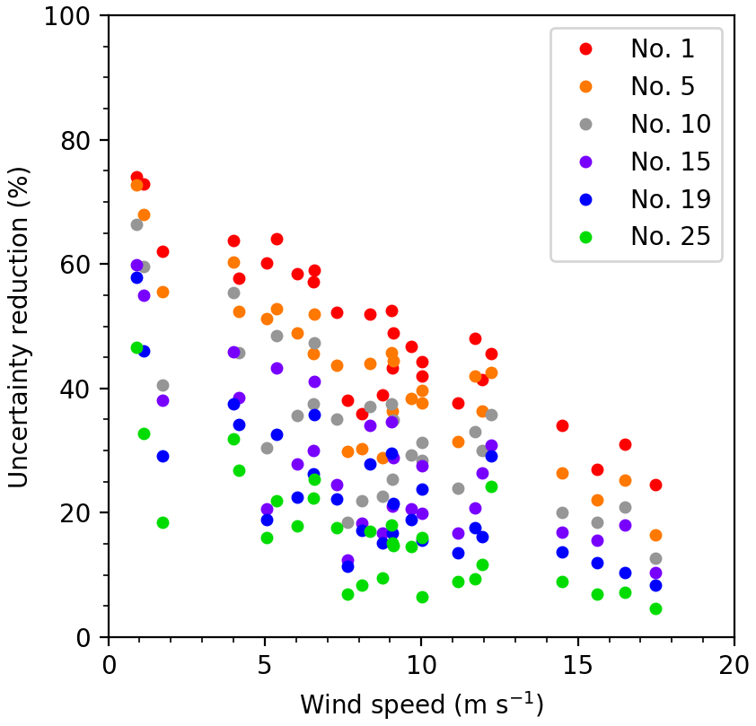
Figure 1 Theoretical uncertainty reduction for the 6 h mean emissions in the PMIF-Paris experiments using the 1st (red), 5th (orange), 10th (light green), 15th (purple), 19th (blue) and 25th (green) best observation sampling from the CarbonSat simulation. The results from the 31 inversion days are given as a function of the average wind speed over the Paris clump. A comparison with the results from Broquet et al. (2018) is given in Fig. S3.

3.2 Potential of space observations for monitoring CO₂ emissions from individual clumps over 3 h time windows

Figure 2a shows the distribution of the number of 08:30–11:30 time windows per clump for which the posterior uncertainty of 3 h mean emissions is smaller than 20 % (this number is called N20) in Exp-NoCor. Clumps with small emission budgets tend to have lower N20 values than those with large budgets, due to the fact that the atmospheric plume generated by small emission clumps is difficult to distinguish from the measurement noise. Typically, N20 is smaller than 5 d for clumps emitting less than 2 MtC yr⁻¹ (like the city of Aswan, Egypt). Conversely, N20 is larger than 10 d for clumps emitting more than 2 MtC yr⁻¹ (like the cities of Manchester, UK; Boston, USA; and Chongqing, China). Note that clumps with emissions larger than 2 MtC, although representing less than 25 % of the total number of clumps, contribute more than 83 % of the total clump emissions. At regional scale (Figs. S4, S5), South America, North America, and Africa tend to have larger N20 values for same bin of clump annual emission than the other regions, while the Middle East and Asia have the lowest ones. In addition, there are large variations and spatial heterogeneity in the N20 values within each emission bins (Fig. S5), which will be further discussed in Sect. 4.

We also show the numbers of 08:30–11:30 time windows per clump being labeled as “well-constrained” when the posterior uncertainty of 3 h mean emission is smaller than other thresholds, e.g., 10 % and 30 % (Fig. 2b). In general, using a posterior uncertainty larger than 20 % as a threshold, we could expect more “well-constrained” cases. But for a given threshold, we still find the number of well-constrained cases increases with the emission budgets.

Figure 3 shows the posterior uncertainty in the clump emissions for the “well constrained” 08:30–11:30 time windows (identified in Exp-NoCor) from different OSSEs. It confirms that in all OSSEs, the posterior uncertainties for clumps with larger emissions are smaller than those with lower emissions. Within a given bin of clump annual emission, the posterior uncertainties from the various OSSEs are very similar, even though they are obtained with different hypotheses regarding the temporal auto-correlation in the prior uncertainty. The interpretation is that, for the inversion of the 3 h emissions before a given satellite overpass, most of the constraint is imposed by the direct satellite observations during this overpass. These observations are independent on different days, and the constraints on different days are not strongly crossed even when errors in the prior estimate are highly correlated in time. However, although small, the impact of temporal auto-correlations in the prior uncertainties can be seen. For example, the posterior uncertainties in ASS (SCS) are systematically smaller than those in AMS (MCS), which confirms that the capability of the inversion system to use the information from observations from previous or subsequent days to reduce the posterior uncertainties increases with the temporal auto-correlations. In SectCS, the posterior uncertainties are smaller than those in MCS and SCS in most regions (Fig. S5), due to the fact that the uncertainty in industrial emissions has a long temporal auto-correlation (τ₂=180 d).

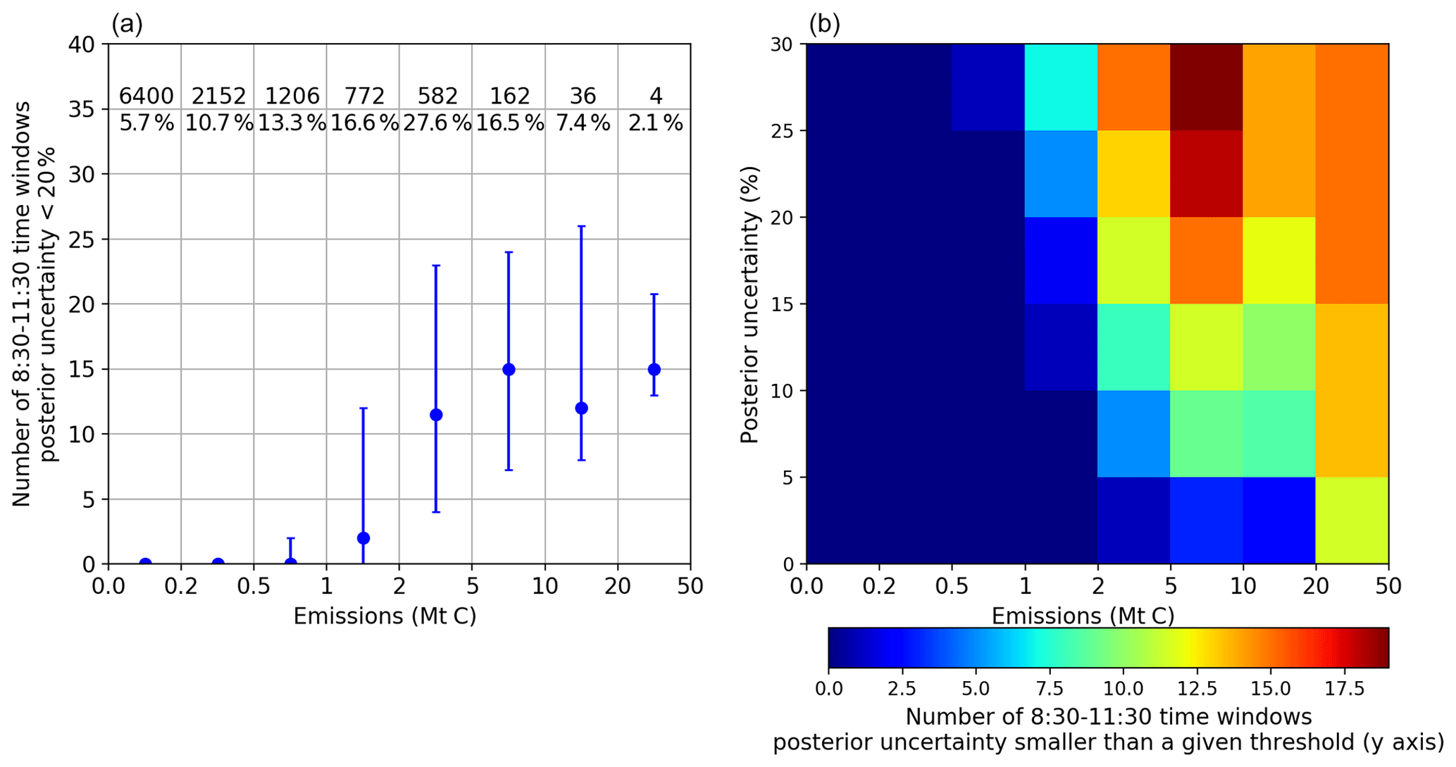
Figure 2 (a) Number of 08:30–11:30 time windows within a year for which the 3 h emissions are constrained with a posterior uncertainty less than 20 % (N20) in the Exp-NoCor experiment. The results are binned according to clump annual emission with bin limits given on the x axis of the figure. Dots and error bars are the median and interquartile range of N20 for all clumps within the emission bin. Numbers at the figure top indicate the number of clumps and the percentage of clump emission within each bin. (b) Number of 08:30–11:30 time windows (color) within a year for which the 3 h emissions are constrained with a posterior uncertainty less than a given threshold (y axis) in the Exp-NoCor experiment.

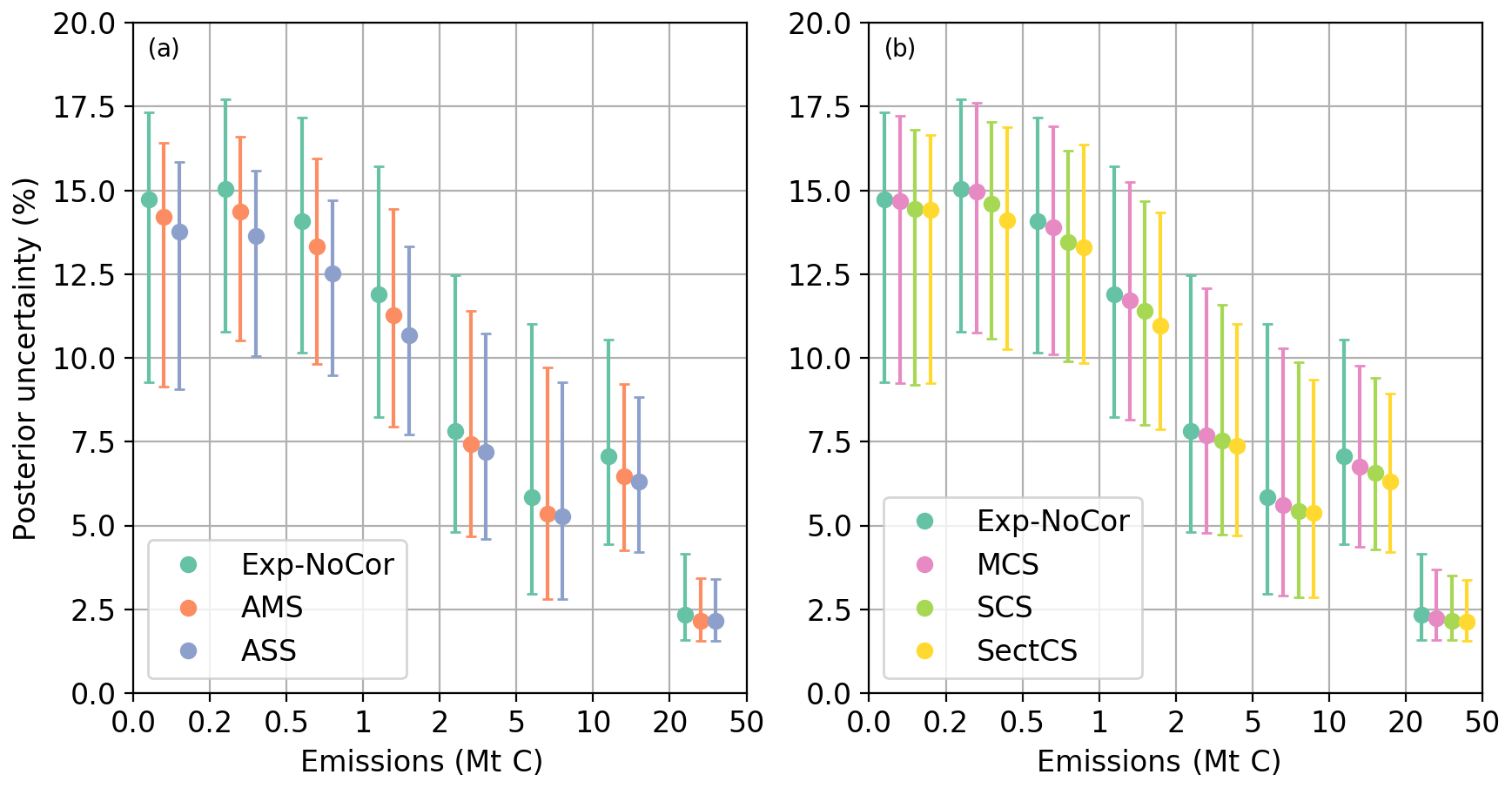
Figure 3 Distribution of the posterior uncertainty in the 3 h mean emissions during the 08:30–11:30 time windows (for which the posterior uncertainty in 3 h mean emissions are smaller than 20 % in Exp-NoCor) obtained with different OSSEs. Dots and error bars are the median and interquartile range. The results are binned according to the clump annual emission with bin limits given on the x axis of the figure. Numbers at the figure top indicate the number of clumps and the percentage of clump emission within each bin.

3.3 Potential of space observations for monitoring daily CO₂ emissions

In previous sections, we analyzed the uncertainty reduction and the posterior uncertainty for the 3 h emissions that generate the atmospheric plume observed from space at 11:30. We now analyze the potential to monitor the daily emission, relying on the extrapolation of constraints on emissions between 08:30 and 11:30 using temporal auto-correlation of the prior uncertainties in step 2 of the inversion (Sect. 2.7.2). Figure 4 shows the distribution of the number of days when the posterior uncertainties in daily emissions are smaller than 20 % (D20) for the same bins of emission clumps as in the previous section. Similar to the distribution of N20, clumps with small emission budgets tend to have lower D20 values than those with large budgets, due to having smaller signal-to-noise ratios for clumps with smaller emissions. The D20 values also strongly depend on the temporal auto-correlation in the prior uncertainty. When no correlation (Exp-NoCor) or short correlation (MCS) are assumed, D20 remains zero even for the largest clumps, since most of the daily emissions are disconnected from the 3 h emissions that are constrained by the satellite observation and keep on bearing the large prior uncertainties associated with the Exp-NoCor and MCS scenarios. When significant temporal auto-correlations (e.g., in the case of AMS, ASS and SCS) are assumed, the results get better and the posterior uncertainties for the daily emissions become less than 20 % for more than 100 d for clumps emitting more than 5 MtC yr⁻¹. At regional scale (Fig. S6), the distribution of D20 values shows a similar pattern to N20: North America, South America and Africa have larger D20 values than the Middle East and Asia for same bin of clump annual emission. But the distribution D20 values in SectCS have large regional variations, reflecting the regional differences in the share of emissions from different sectors.

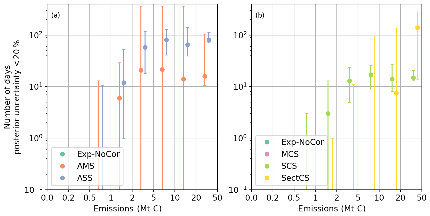
Figure 4 Number of days within the year when the posterior uncertainty of daily emissions is smaller than 20 % (D20). The results are binned according to the clump annual emission with bin limits given on the x axis of the figure. Note that the median values of D20 for all clumps in Exp-NoCor and in MCS, for clumps whose annual emissions are between 0.5 and 1 MtC in AMS, ASS and SCS, and for clumps whose emissions are below 10 MtC in SectCS, are all zero, so that the dots in these cases are not visible on the y axis with log scale. The dots and error bars are the median and interquartile range of D10 for all clumps within the emission bin. Numbers at the figure top indicate the number of clumps and the percentage of clump emission within each bin.

3.4 Potential of space observations for monitoring annual CO₂ emissions

We now analyze the results for the annual emissions, allowed again by the derivation of the posterior uncertainty covariance matrix A for individual clumps in step 2 of the inversion, and thus the aggregation of the posterior uncertainties in time. Figure 5 shows the posterior uncertainties in annual emissions from the OSSEs. When we assume that there is no temporal auto-correlations in the prior uncertainties, the uncertainties obtained from the inversions remain very close to the prior uncertainties (30 %) for all emission bins since the information from the few well-constrained 08:30–11:30 time windows within the year is not extrapolated to the huge unobserved fraction of the total annual emission over the year. The benefit of satellite observations becomes apparent when assuming that the prior uncertainties have temporal auto-correlations. Similar to the posterior uncertainties for 3 h emissions during 08:30–11:30, the posterior uncertainties in annual emissions are smaller in the OSSEs where the prior uncertainties have stronger temporal auto-correlation. This indicates that temporal auto-correlations help to extrapolate the information on the emissions from the satellite passes over a given clump to emissions during other hours and days when there are no direct observations. Small clumps tend to have a larger relative posterior uncertainty in annual emissions than large clumps even when temporal error correlations are accounted for. The posterior uncertainties in the annual emissions of large cities with annual emission >5 MtC yr⁻¹ can be constrained to better than 20 % in AMS, SCS and SectCS, and to better than 10 % in ASS. On the other hand, the posterior uncertainties for small emission clumps with annual emissions <0.5 MtC yr⁻¹ are always larger than 15 %, regardless of the temporal auto-correlations in prior uncertainties.

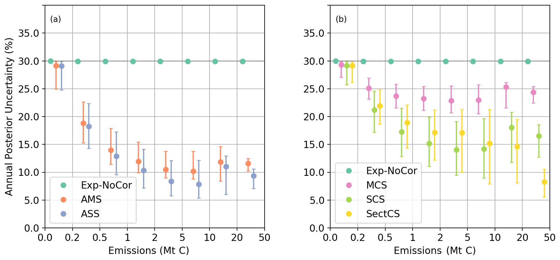
Figure 5 Distribution of the posterior uncertainties in annual CO₂ emissions for different OSSEs. The results are binned according to the clump annual emission with bin limits given on the x axis of the figure. Dots and error bars are the median and interquartile range of posterior uncertainty. Numbers at the figure top indicate the number of clumps and the percentage of clump emission within that bin.

4 Discussion and conclusions

PMIF provides information on the potential of space-borne imagery to constrain CO₂ emissions from emission clumps over the globe from scales of a few hours to the annual scale. It uses a simple Gaussian plume model to relate the emissions and the XCO₂ plumes. This is a strong simplification of the physics which impacts the range of uncertainties that can be accounted for in the inversion problem, but a preliminary evaluation against a more complex setup (that of Broquet et al., 2018) indicates that it provides the correct order of magnitude for the uncertainties in the inverted emissions for an individual city: Paris.

In this study, we focused on the projection of uncertainties in satellite observations on the uncertainty of inverted emissions. Some sources of uncertainties that could have some impacts on the inversions when dealing with real data are ignored. Firstly, the plumes generated by the Gaussian plume model are straight along the wind direction at the source pixel. As a result, we allow the plumes from nearby clumps to potentially cross each other, but these plumes will systematically diverge over long distances. The Gaussian plume model cannot reproduce plumes overlapping along the atmospheric circulation like Eulerian transport models. In this sense, the overlapping effect of plumes can be underestimated in PMIF. In a realistic situation of atmospheric transport, if plumes from multiple clumps overlap very often, the inversion performance for individual clumps will be degraded since it will have difficulties accurately attributing the XCO₂ signals to individual clumps. Furthermore, we assume that the Gaussian plume model can perfectly link the emissions and XCO₂ and ignore the transport model error. If forced with erroneous wind fields, the simulation of XCO₂ plumes can have the wrong shape and location and thus generate large uncertainties in the inversions. In the inversion with actual XCO₂ observations from OCO-2, Nassar et al. (2017) allowed the wind direction to change from the wind re-analysis used to force the Gaussian plume model, if it improved the fit between simulated plumes and the observed signals. Reuter et al. (2019) and Kuhlmann et al. (2019) showed that the co-located NO₂ satellite observations could help to detect and constrain the location and shape of XCO₂ plumes. The transport model error may be partly reduced by incorporating additional information from other tracers when fitting the model to real data, but it is unknown to what extent these additional constraints are useful to improve the inversion of CO₂ emissions from cities and point sources. With the current design of PMIF, the impact of transport error is hard to evaluate. Secondly, we ignore systematic measurement errors from the XCO₂ imagery. Broquet et al. (2018) showed that systematic error could hamper the ability of the inversion system to reduce the errors in the emissions estimates. Thirdly, we neglect the impact of uncertainties in diffuse fossil fuel CO₂ emissions (outside clumps) and non-fossil CO₂ fluxes (within and outside clumps), the latter including net ecosystem exchange (NEE) from the terrestrial biosphere, the CO₂ emitted by the burning of biofuel, the respiration from humans and animals (Ciais et al., 2020), and the net CO₂ fluxes between the atmosphere and ocean. For example, the signals from terrestrial NEE can be strong during the growing season, and the signals from ocean CO₂ fluxes may have a critical impact on the overall XCO₂ patterns in proximity to coastlines. In principle, the signals of diffuse fossil fuel CO₂ emissions and non-fossil CO₂ fluxes outside the clumps can be potentially filtered by removing the local background XCO₂ field to extract plumes generated only by emissions from clumps (Kuhlmann et al., 2019; Reuter et al., 2019; Ye et al., 2020; Zheng et al., 2020). The non-fossil CO₂ fluxes within clumps vary from clump to clump and could contribute a non-negligible fraction of the total CO₂ fluxes in many clumps (Bréon et al., 2015; Ciais et al., 2020; Wu et al., 2018). The satellite observations alone cannot effectively differentiate the fossil fuel CO₂ emissions and the non-fossil CO₂ fluxes within clumps. Fourthly, the PMIF system controls the scaling factors for the mean emissions of daily 3 and 21 h windows and for each clump, ignoring uncertainties in the spatial distribution and temporal profile of the emissions (described by the operator M_inventory) within the clumps and over the time windows. Such uncertainties are called aggregation errors (Wang et al., 2017; Wu et al., 2011). However, Broquet et al. (2018) compared the results of inversions using the realistic spatial distribution of emissions and using a homogenous one over two discs with a different radius for M_inventory and found that having imperfect spatial distribution of emissions to model M_inventory (thus the aggregation error) only has a small impact on the uncertainties and errors in the inverted emissions. Future developments in PMIF should attempt to quantify the impacts of such sources of uncertainties, while keeping its power of constraining the emissions from a large range of sources with global coverage.

Although it ignores the sources of uncertainties listed above, the current PMIF can still be used to investigate the impacts of some key parameters of the inversion problem and to allow, for the first time, a first-order extrapolation of the results from single-city studies to all significant emission clumps over the globe and under a full range of meteorological conditions during a year.

The key result summarized in Fig. 2 is that using a single CO2M satellite, only the clumps with annual budget higher than 2 MtC yr⁻¹ (e.g., Manchester, UK, Boston, USA and Chongqing, China) can potentially be well constrained with N20 being larger than 10 within a year. However, there are large variations in the N20 values for clumps with such levels of emission. Figure 6a and b show the maps of the number of observations within each $\mathrm{2}{}^{\circ }\times \mathrm{2}{}^{\circ }$ grid cell during 1 year in the USA and China, which is an indicator for the frequency of clear-sky days: the larger the number of observations, the higher the frequency of clear-sky days. It is clearly seen in Fig. 6c and d that the clumps in southern China have low N20 values when they are located in areas with a low frequency of clear-sky days. For clumps that have emissions between 2 and 5 MtC yr⁻¹, N20 values are below 10 d in a cloudy/hazy region like southeastern China and are close to 30 d in a clear-sky region like the western coast of the USA. These results illustrate the dependence of the potential of satellite observations to constrain emissions on the frequency of clear-sky conditions. The relative uncertainty in the inversion of the emissions from a clump is primarily driven by the budget of these emissions, and by the wind speed (as illustrated by Fig. 1). The frequency of clear-sky days modulates the number of direct observations of the plume from a clump and thus the number of days for which the inversion can decrease the uncertainty when ignoring temporal auto-correlations in the prior uncertainty in Exp-NoCor. The frequency of clear-sky days, together with the emission rate and wind speed, are the main drivers of the posterior uncertainty in daily to annual emissions when accounting for temporal auto-correlations in the prior uncertainty.

Figure 6 Number of observations in $\mathrm{2}{}^{\circ }\times \mathrm{2}{}^{\circ }$ grid cells during 1 year (a, b) and N20 values (c, d).

We showed that one CO2M imager can provide a direct constraint for the estimate of emissions from clumps with emissions larger than 2 MtC yr⁻¹, but over limited periods only. N20 is smaller than 25 for most clumps, indicating that even for emissions during 08:30–11:30, one cannot expect more than 25 d when the CO2M observations sample the plumes from clumps with a sufficient number of observations (Fig. 2) during 1 year. The use of a constellation of CO2M satellites in the current plan could potentially improve the frequency of good samplings. Imaging from geostationary orbit (GEO) imagers like NASA's GeoCarb mission (O'Brien et al., 2016; Polonsky et al., 2014) could offer sampling during different periods within a day to constrain the diurnal profile of emissions. Highly elliptical orbit (HEO) imagers could also provide observations at northern high latitudes with a similar high frequency to GEO (Nassar et al., 2014). However, even though multiple space-borne platforms can sample the plumes more frequently, the satellites using passive sensors like that planned for CO2M can never sample the plumes under cloudy/hazy conditions.

We also investigated the possibility of extrapolating the information obtained from the time windows for which the emissions are constrained by satellite observations to estimate emissions on other hours, days and throughout a year. Such an extrapolation relies on the model of the emission inventories used as a prior of PMIF, that is, in the framework of PMIF, the temporal auto-correlation of the uncertainty of prior emissions. The analysis of posterior uncertainties in the 3 h mean emissions, in daily emissions and in annual emissions all show that the configuration of this temporal auto-correlation has a large impact on the inversion results. For example, posterior uncertainties in annual emissions range from less than 10 % with strong auto-correlation (ASS) to 25 % with medium auto-correlation (MCS) for clumps with emissions higher than 2 MtC yr⁻¹. The orders of magnitude in the posterior uncertainty will be critical to the objective assessment of annual emissions. However, since state-of-the-art emission products rarely report their uncertainties and temporal auto-correlations (Andres et al., 2016; Gurney et al., 2019), it is difficult to exclude any configuration of OSSEs in this study. The strong impact of the prior uncertainty on the inversion results thus highlights the priority of future research to systematically assess the uncertainty, especially the temporal error co-variances, in the emission products.

Even if emissions can be effectively constrained by CO2M for clumps whose emissions are larger than 2 MtC yr⁻¹, the sum of annual emission budgets from these large clumps account only for 54 % of the total CO₂ clump emissions and for 36 % of the total global fossil fuel CO₂ emissions (accounting for diffuse emissions outside the clumps), according to the clump definition of Wang et al. (2019) and the ODIAC emission map. For a specific country, clumps with emissions larger than 2 MtC yr⁻¹ typically represent less than 50 % of the total national emissions (accounting for diffuse emissions outside the clumps). It thus shows the difficulty of using a single CO2M imager as the only source of information to constrain national emissions. This limitation of a single CO2M imager calls for innovations to integrate other types of observations in inversion systems to improve the ability to estimate emissions at both city scale (Lauvaux et al., 2016; Sargent et al., 2018; Staufer et al., 2016) and larger spatial scales (Palmer et al., 2018; Wang et al., 2018a).

Appendix A: Acronyms

AMS:	Annual component and moderately correlated sub-annual component
ASS:	Annual component and strongly correlated sub-annual component
CDIAC:	Carbon Dioxide Information Analysis Center
CNES:	Centre National d'Etudes Spatiales
CO2M:	Copernicus Anthropogenic Carbon Dioxide Monitoring
D20:	Number of days within the year when the posterior uncertainty of daily emissions is smaller than 20 %
ECMWF:	European Centre for Medium-Range Weather Forecasts
ESA:	European Space Agency
EUMETSAT:	European Organisation for the Exploitation of Meteorological Satellites
GOSAT:	Greenhouse Gases Observing Satellite
MCS:	Moderately correlated sub-annual component
N20:	Number of 08:30–11:30 time windows per clump for which the posterior uncertainty of 3 h mean
	emissions is smaller than 20 %
NoCor:	No temporal auto-correlation
OCO:	Orbiting Carbon Observatory
ODIAC:	Open-source Data Inventory for Anthropogenic CO2
OSSE:	Observing System Simulation Experiment
PMIF:	Plume Monitoring Inversion Framework
SCS:	Strongly correlated sub-annual component
SectCS:	Sector-dependent correlated sub-annual component
SZA:	Solar zenith angle
TIMES:	Temporal Improvements for Modeling Emissions by Scaling
XCO2:	Vertically integrated columns of dry-air mole fractions of CO2