the Creative Commons Attribution 4.0 License.
the Creative Commons Attribution 4.0 License.
 | 26 Nov 2020
Necessary conditions for algorithmic tuning of weather prediction models using OpenIFS as an example
Pirkka Ollinaho
Madeleine Ekblom
Vladimir Shemyakin
Heikki Järvinen
Algorithmic model tuning is a promising approach to yield the best possible forecast performance of multi-scale multi-phase atmospheric models once the model structure is fixed. The problem is to what degree we can trust algorithmic model tuning. We approach the problem by studying the convergence of this process in a semi-realistic case. Let M(x, θ) denote the time evolution model, where x and θ are the initial state and the default model parameter vectors, respectively. A necessary condition for an algorithmic tuning process to converge is that θ is recovered when the tuning process is initialised with perturbed model parameters θ′ and the default model forecasts are used as pseudo-observations. The aim here is to gauge which conditions are sufficient in a semi-realistic test setting to obtain reliable results and thus build confidence on the tuning in fully realistic cases. A large set of convergence tests is carried in semi-realistic cases by applying two different ensemble-based parameter estimation methods and the atmospheric forecast model of the Integrated Forecasting System (OpenIFS) model. The results are interpreted as general guidance for algorithmic model tuning, which we successfully tested in a more demanding case of simultaneous estimation of eight OpenIFS model parameters.
- Article
(2872 KB) - Full-text XML
- BibTeX
- EndNote


Numerical weather prediction (NWP) models solve non-linear partial differential equations in discrete and finite representation. Subgrid-scale physical processes, such as cloud microphysics, are treated in specific closure schemes. Once the model structure is fixed, some parametric uncertainty remains depending on how closure parameter values are specified. Closure schemes are always simplified representations of the real world, so “universally true” parameter values do not exist. This uncertainty can be conceived as a probability density of the closure parameters: the expected value corresponds to the optimal model skill and the covariance to their inherent uncertainty. The expected parameter value is the obvious choice for deterministic forecasting while the covariance can be utilised to represent parametric uncertainty in ensemble forecasting (Ollinaho et al., 2017).
Model tuning is an attempt to unveil some statistics of the probability density of the closure parameters, and algorithmic methods add objectivity and transparency to the process (Hourdin et al., 2017; Mauritsen et al., 2012). It is paramount in algorithmic model tuning that the method applied is able to converge to the correct statistics with limited computing resources.
The aim of this paper is to gauge the circumstances favouring successful model tuning when ensemble-based parameter estimation methods are used. These include, for instance, differential evolution (Storn and Price, 1997) and its variants, genetic algorithm (Goldberg, 1989), particle swarm optimisation (Kennedy, 2010) and Gaussian importance samplers (e.g. the ensemble prediction and parameter estimation system, EPPES; Järvinen et al., 2012; Laine et al., 2012). The results may also be useful for more deterministic algorithms, such as multiple very fast simulated annealing (Ingber, 1989), and filter-based estimation algorithms such as ensemble Kalman filter and its variants (e.g. Annan et al., 2005; Pulido et al., 2018) as well as particle filters (e.g. Kivman, 2003). Of course, the length of the time window is limited in filter-based estimation methods.
The results are interpreted so as to provide guidance on successful tuning exercises and savings in computing time. Convergence testing is always semi-realistic and can provide insight on how to design fully realistic model tuning exercises. Based on a very large amount of tests, the following general guidance can be drawn up.
Trivial testing. It is important to start model optimisation with some trivial testing before proceeding to more demanding realistic cases. In a recommended trivial test, model parameters are offset slightly from their default values and optimisation is confined to a known training sample of model initial states and forecasts. In this case, the chosen optimisation method must be able to recover the default parameter values. If the optimisation target (cost function) is too simplistic, the process may not converge or convergence is very slow. In the case of ensemble-based sampling, we noted that stochastic initial state enhances the recovery of the parameters.
Efficiency. It is important to consider how to efficiently allocate computing resources. We noted that it is better to perform a long convergence test with a small ensemble and varying initial states rather than a short test with a large ensemble; the variability of atmosphere is thus more robustly sampled. Also, in the atmospheric forecast model of the Integrated Forecasting System (OpenIFS), it turned out that already a 24 h forecast range is sufficiently long for parameter convergence, offering potential savings in computing time.
Reproducibility. It is usually necessary that in realistic testing, the optimisation result is verified in an independent sample. With the convection parameters of OpenIFS used in this study, reproducibility is better for a relatively short forecast range (24 h). At longer ranges, results are less repeatable. Thus, from both the efficiency and reproducibility viewpoints, a 24 h forecast range seems optimal for the convection parameters used in this study.
Practical concerns. Our testing showed that one should not blindly trust algorithmic tuning – it is an efficient tool that can potentially accelerate model development (Jakob, 2010), but it must be used cautiously. For example, ensemble-based sampling works well in fine tuning of an already well-performing model but less well if the initial uncertainty of model parameters is large. It is also worth noting the deep-rooted ambiguity in the optimal parameter values which can depend on the forecast range.
The paper contains the following sections: Sect. 1 introduces the topic of convergence testing, Sect. 2 presents tools and methods needed for running and evaluating convergence tests, Sect. 3 presents the convergence test setups, Sect. 4 presents the results, Sect. 5 contains further discussion, and Sect. 6 concludes the paper.
2.1 OpenIFS and closure parameters of the convection scheme
OpenIFS is the atmospheric forecast model of the ECMWF IFS. In this study, we use a version based on the model version that was operational from November 2013 to May 2015 (cycle 40r1; ECMWF, 2014). Convergence tests are run at two resolutions: TL159 and TL399, corresponding to approximately 125 and 50 km resolutions, respectively, both with 91 vertical levels. Initial conditions are produced closely following what is done in the operational ECWMF IFS ensemble (Ollinaho et al., 2020) for the year 2017 to cover different weather regimes and seasons. Each convergence test contains 52 ensemble forecasts; i.e. an ensemble is initialised once per week. The data set of ensemble initial conditions (containing a control member plus 50 perturbed analyses) has been generated with IFS cycle 43r3. Thus, some spinup/spindown is possible at early forecast ranges of a few hours. The differences between the two model versions can be found in ECMWF (2019).
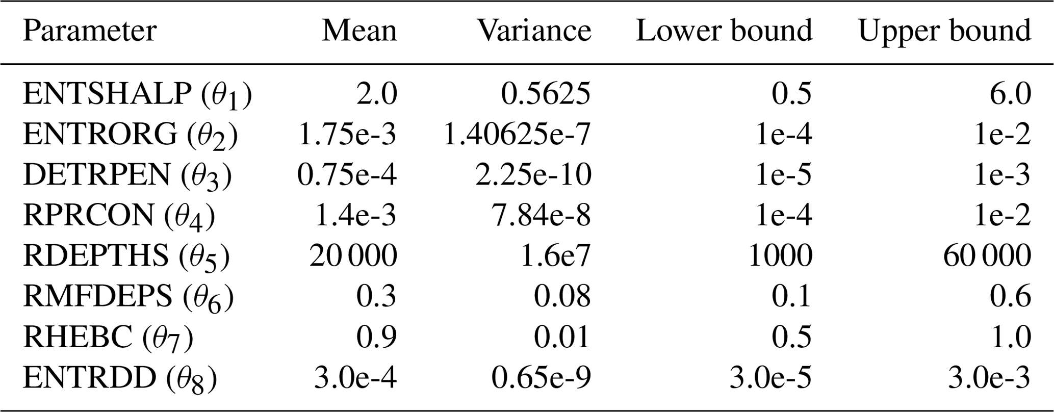
We focus on closure parameters of the convection scheme, consisting of a bulk mass flux with an updraught and downdraught pair in each grid box for shallow, deep and mid-level convection (ECMWF, 2014; Bechtold et al., 2008). The parameters, their default values and short descriptions are in Table 1. The tests also involve the use of a stochastic representation of model uncertainty: stochastically perturbed parameterisation tendency (SPPT; Palmer et al., 2009).
Table 1Parameters of the convection scheme of OpenIFS. θ1 and θ2 are used the most in this study.

2.2 OpenEPS – ensemble prediction workflow manager
Convergence tests involve running large amounts of ensemble forecasts. Traditionally, ensemble forecasting and research on ensemble methods have been tied to major NWP centres providing operational ensemble forecasts to end users. Usually, these platforms are not suited for academic research. Instead, we use a novel and easily portable ensemble prediction workflow manager (called OpenEPS), developed at the Finnish Meteorological Institute specifically for academic research purposes (https://github.com/pirkkao/OpenEPS, last access: 19 November 2020).
OpenEPS has been designed for launching, running and post-processing a large number of ensemble forecast experiments with only a small amount of manual work. OpenEPS is very flexible and can be easily coupled with external applications required in parameter tuning, such as autonomous parameter sampling.
2.3 Optimisation algorithms
Brute force sampling of the parameter space of full-complexity NWP models is computationally far too expensive. Typically, one can afford running perhaps only some tens or a maximum of a few hundred simulations in a tuning experiment. Therefore, the tuning methods need to be sophisticated. In these convergence tests, we use two ensemble-based optimisation algorithms: EPPES (Laine et al., 2012; Järvinen et al., 2012) and differential evolution (DE) (Storn and Price, 1997; Shemyakin and Haario, 2018).
EPPES is a hierarchical statistical algorithm which uses Gaussian proposal distributions, importance sampling and sequential modelling of parameter uncertainties to estimate model parameters. A parameter sample is drawn from the distribution, an ensemble forecast is run with these parameter values, and the goodness of the parameter values is evaluated by calculating a cost function for each ensemble member. The proposal distribution is sequentially updated such that it shifts towards more favourable parameter values. Here, the shift of parameter mean values between consecutive iterations is limited to a conservative value of 5 %.
DE (Storn and Price, 1997) is heuristically based on natural selection. It consists of evolving population of parameter vectors where vectors leading to good cost function values thrive and produce an offspring, while vectors leading to bad cost function values are eliminated. The population update procedure of DE is achieved by a certain combination of mutation and crossover steps. These steps ensure that the new parameter vectors differ at least slightly from the vectors that already belong to the population. The natural selection is achieved through the selection step, where the elements of the current population compete with the new candidates based on the defined cost function. The fittest are kept alive and proceed to the next generation. Besides the standard DE algorithm, we use generation jump (Chakraborty, 2008), DE/best/1 mutation strategy (Feoktistov, 2006; Chakraborty, 2008; Qing, 2009) with randomised scale factor by jitter and dither (Feoktistov, 2006; Chakraborty, 2008) and recalculation step (Shemyakin and Haario, 2018). Jitter and dither act to increase the diversity of the parameter population so that they cause small random variation in the parameter values preventing DE from sticking to some specific values. Jitter corresponds to the approach when the scale factor is randomised for every mutant parameter vector in the mutation process by sampling from the given (usually uniform) distribution. Dither corresponds to the approach when the fixed scale factor is slightly randomised for each single component of the mutant vector in the mutation process. The recalculation step enhances the convergence when the cost function is stochastic. This means that occasionally the parameter vector is not updated but passed for a new iteration in order to ensure that only those parameter vectors leading to good scores for two times are used in generation of new vectors.
The main focus here is on the EPPES results. More details about the algorithms and their specific settings are explained in Appendices A1 and A2.
2.4 Optimisation target functions
We will apply two very different optimisation target functions (hereafter cost functions) in the convergence tests. The first one is the global root mean squared error of the 850 hPa geopotential height (ΔZ):
where Z850 and denote 850 hPa geopotential in the pseudo-observations and perturbed forecast at each grid point. D denotes the horizontal domain. Pseudo-observations are default model forecasts with fixed default parameter values. Full fields are three-dimensional but for ΔZ only two-dimensional slices are used. This is a restrictive cost function formulation and used here merely as a useful demonstrator. There are three reasons why we expect ΔZ to perform sub-optimally. First, it exploits information only from a small fraction of the model domain and the upper parts of the model domain remain unconstrained. This means that ΔZ is not (directly) sensitive to perturbations in the middle and upper troposphere where the most influential effects of perturbed convection are present. Second, it requires substantial interpolation of forecasts and reference data because OpenIFS has a terrain-following hybrid-sigma vertical coordinate, and hence the model levels are not aligned with pressure levels in lower troposphere. Third, the 850 hPa level intersects with the ground level in mountainous areas.
The second cost function is the global moist total energy norm (ΔEm, e.g. Ehrendorfer et al., 1999) and it is a very comprehensive integral measure of the distance between two atmospheric states. The moist total energy norm can be written as
where u′, v′, T′, q′ and refer to differences between forecast and pseudo-observations in wind components, temperature, specific humidity and the logarithm of surface pressure. Ma is the mass of the atmosphere, cq is a scaling constant for the moist term, L vaporisation energy of water, cp specific heat at constant pressure, Tr reference temperature and pr reference pressure. Here, we set Tr=280 K and pr=1000 hPa as in Ollinaho et al. (2014). D and η denote increments of horizontal and vertical integrals. Unlike in Ollinaho et al. (2014), we set cq to 1 and dη to equal the difference of pressure between consecutive model levels. Ollinaho et al. (2014) also show instructions how to discretise ΔEm for practical use.
We expect that at short forecast ranges, the linkage between variations in the values of ΔEm and parameter perturbations is detectable, enabling us to estimate parameter densities.
2.5 Evaluation of convergence tests
The parameter convergence is measured with fair continuous ranked probability score (fCRPS; Ferro et al., 2008) formulated as the kernel representation (see, e.g. Leutbecher, 2018). fCRPS rescales the scores as if the ensembles were infinitely large so that there is no dependence between ensemble size and the score itself. The property of fairness is essential in comparison of convergence tests with different ensemble sizes. fCRPS has not been designed for evaluation of ensembles of parameter values, so a direct application of fCRPS may lead to cancellation of the two terms (see Eq. 6; Leutbecher, 2018) causing difficulties in interpreting the results. Therefore, we use the two terms separately for each parameter θn:
and
where n is the index over tunable parameters, and are the parameter values used by ensemble members j and k, θd,n is the default parameter value, and M is the ensemble size. Each ensemble member is run with a unique set of parameter values. The first part (Eq. 3) is a measure of how much the ensemble mean parameter value differs from the default value, while the second part (Eq. 4) indicates how much spread is associated with the ensemble mean parameter value; in other words, it indicates how certain or uncertain the algorithm considers the parameter value. Both parts of fCRPS have a perfect score of zero.
Table 2 shows the outline of our experiments. The table explains the different levels of complexity we use in the convergence tests. The different levels of complexity are tested to see which is the optimal way to extract information of the parameter space. On the one hand, keeping convergence tests as simple as possible makes interpretation of the test results easy, but on the other hand, more complex tests provide information on how the parameter tuning system would perform in fully realistic tuning tasks.
Table 2Summary of convergence tests with different degrees of complexity.
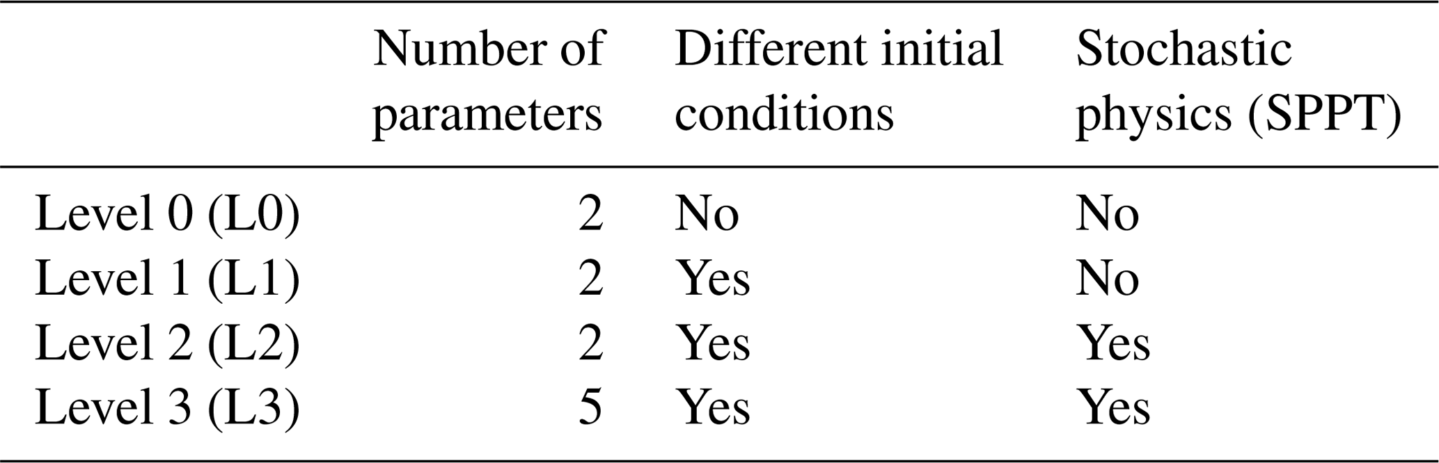
L0, L1 and L3 tests are performed with one setup: a forecast range of 48 h and an ensemble size of 50 members. ΔZ is only tested at the L1 level. Most of the effort is put on L2 testing with ΔEm so they are performed with various combinations of forecast range and ensemble size. The focus is on L2 tests on one hand because we assume that if the convergence is good at this level of complexity, it will be good also at lower levels. On the other hand, convergence in L2 and L3 tests is relatively similar. We use the parameters θ1 and θ2 in L0 to L2 tests and parameters θ1 to θ5 in L3 tests. In L0 tests, all forecasts are initialised from an unperturbed initial state of the control forecast (1 January 2017, 00:00 UTC). L1, L2 and L3 tests use ensemble initial conditions from 52 dates.
Throughout the paper, the pseudo-observations are generated with a default model with fixed parameter values (see Table 1). Therefore, the target of the convergence is always known (i.e. the default parameter set), and it stays the same during the tests. Analyses, reanalyses or real observations are not used in this study.
For brevity, we mainly concentrate on discussing results obtained with EPPES, although most of the convergence tests have been run with both algorithms. Due to the nature of the algorithms, EPPES produces less noise near the end of the convergence tests. Therefore, results generated with EPPES are easier to interpret. However, none of the results produced with DE contradict the results of EPPES.
4.1 Selection of level of complexity
We test how much complexity should be included in algorithmic tuning. Figure 1 shows four convergence tests with different levels of complexity, described in Table 2. As expected, the parameters converge slower the higher the level of complexity is as the parameter uncertainties decrease slower. Both parameters converge very fast in the trivial L0 convergence test. Convergence to the default values in the L0 convergence test is trivial as minimisation of the parameter perturbations is the only way to minimise the cost function values. However, we want to emphasise that fully realistic tuning at L0 level of complexity could lead to overfitting of the parameters since the parameters would be optimised for that specific weather state only. L0 can still be used to test that the tuning infrastructure works.
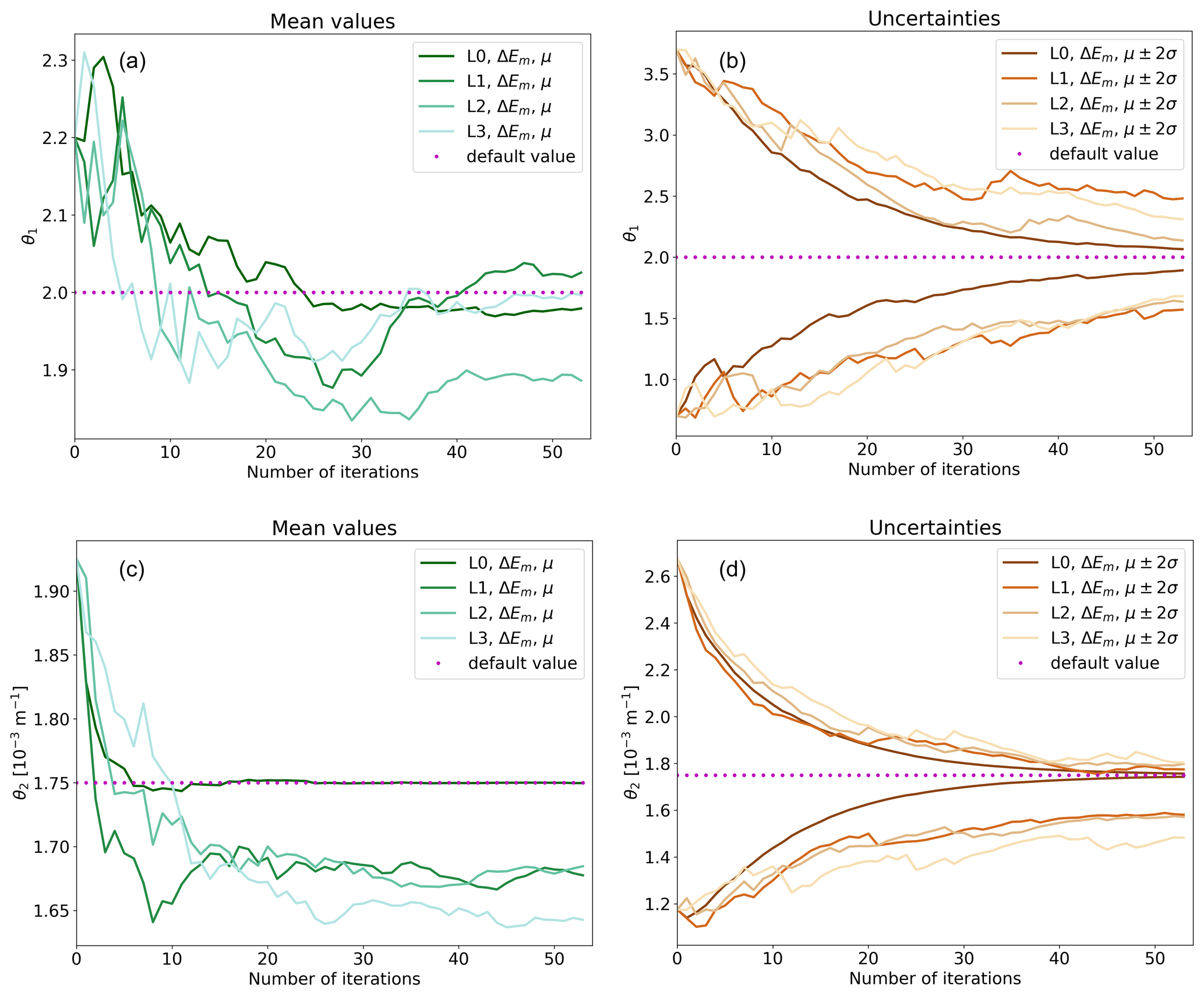
Figure 1Comparison of convergence tests at different levels of complexity. Panels (a) and (b) show the evolution of distribution mean value (μ) and the mean value ±2 standard deviations of uncertainty (μ±2σ) for θ1, and panels (c) and (d) show the same as (a) and (b) but for θ2. The purple dots show the parameter default values. The x axes show running number of iterations, i.e. how many ensemble forecasts have been used. ΔEm is used as the cost function, and the levels of complexity are summarised in Table 2. EPPES is used as the optimiser, the ensemble size is 50 members, and the forecast range is 48 h.
L1, L2 and L3 tests resemble more fully realistic model tuning. Figure 1 shows that the convergence tests at different levels of complexity behave quite reasonably. The uncertainty cannot vanish completely since some uncertainty is always present due to ensemble initial conditions.
L1, L2 and L3 tests have a common feature that the parameters tend to converge to some off-default values. This feature is inherent to convergence tests, which use pseudo-observations generated with the default model. The convergence to off-default values will be discussed further below.
We recommend using L1 (only perturbed initial conditions) in fully realistic model tuning. L1 is the simplest safe option. Higher levels of complexity do not provide additional information; instead, they only make convergence more difficult. L0 is only recommended for testing purposes. Depending on user needs, L1 can be modified by adding more parameters.
4.2 Selection of optimisation target
Here, we compare convergence tests that use different cost functions. Figure 2 compares L1 convergence tests with ΔEm (shown with solid and dash-dotted black lines) and ΔZ (shown with dotted cyan lines and shading in the background). Figure 2 shows that ΔEm leads to much faster convergence than ΔZ. The superior performance of ΔEm is explained by two factors. First, the global integral of several variables catches the signal of parameter perturbations much better than a single level measure. Second, perturbations of convection parameters do not affect 850 hPa geopotential directly, so 48 h may not be long enough to develop a traceable signal. Perturbations of convection parameters modify specific humidity, wind components and temperature directly. These fields must change substantially before the signal is seen in geopotential at 850 hPa.
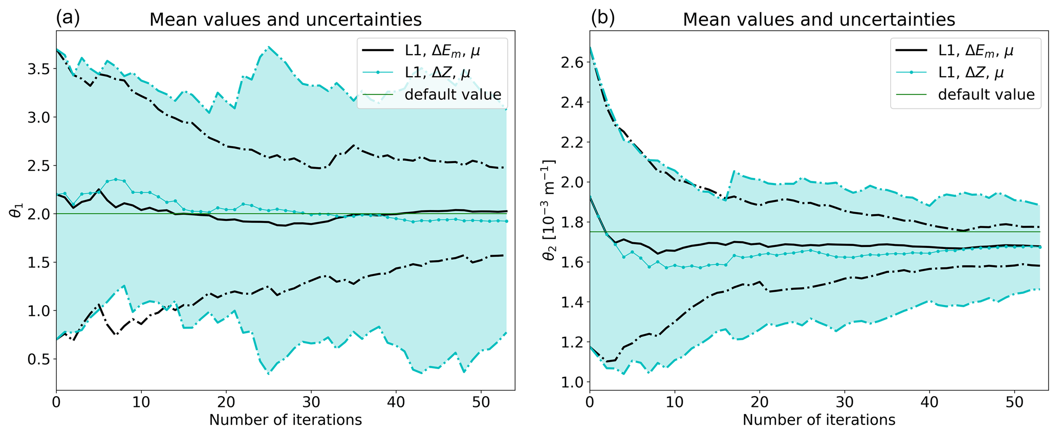
Figure 2Convergence tests with different cost functions: (a) θ1 and (b) θ2. The x axes show running number of iterations. Solid black lines show the evolution of distribution mean values (μ) and dash-dotted black lines the mean values ±2 standard deviations when ΔEm is used as the cost function. Dotted cyan lines and shading in the background show the same for ΔZ. Default value shows the fixed parameter value used in the default model. Both convergence tests are L1 tests with 50 ensemble members and 48 h forecasts. EPPES is used as an optimiser.
We recommend in general using a more comprehensive cost function that accounts for more than one atmospheric level and more than one variable. Targeted forecast range also plays a crucial role in constructing a suitable cost function and thus should be carefully chosen based on what type of parameterised processes are being optimised. However, it is likely that with some other parameters a cost function other than ΔEm might work better.
4.3 Finding the most efficient setup
The process of finding a forecast range and an ensemble size that give satisfactory convergence with a minimal amount of computational resources is done in two steps. First, we compare forecast ranges. Second, we take the forecast range with the fastest convergence in order to find optimal ensemble size using an L2 level of complexity. We expect that the results obtained with such a high level of complexity generalise well to lower levels. This step can also be seen as fine tuning of the cost function.
We take the final parameter values proposed by EPPES to calculate the components of fCRPS (Eqs. 3 and 4). Low bias and low uncertainty are desired since they indicate that the mean value has converged close to the default value and that the uncertainty is small. However, we do not expect precise convergence to the default values because initial condition and model perturbations are activated in the experiments. Figure 3 shows the components of fCRPS of the final ensemble for the parameter θ2 from numerous convergence tests with different forecast ranges and ensemble sizes. From Fig. 3, it is obvious that the convergence of θ2 is the most efficient when the forecast range is 24 h. It is remarkable that 24 h and also 48 h lead to significantly better convergence than 72 h that was used, for example, in Ollinaho et al. (2014). For θ1, 12, 24 and 48 h forecasts are the best and roughly equally good (not shown).
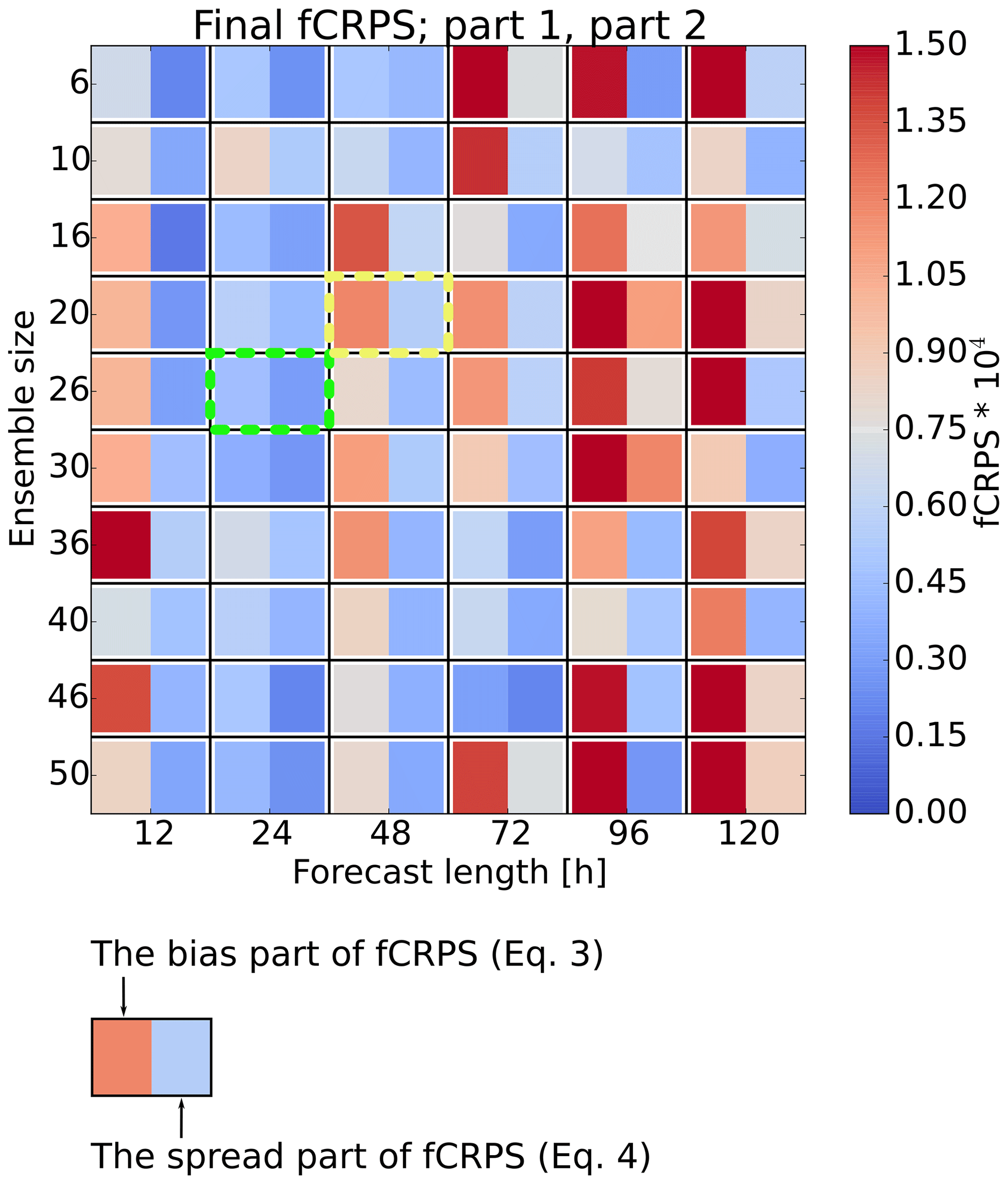
Figure 3Components of fCRPS from the final iteration of the convergence tests with various forecast ranges and ensemble sizes. In this example, the optimisation algorithm is EPPES and the parameter is θ2. The left-hand side of each block represents the average distance of the parameter values from the default value (Eq. 3), and the right-hand side represents the spread of the parameter value distribution (Eq. 4). Low values and blue colours of both sides of the blocks indicate good convergence. Green and yellow boxes highlight the tests repeated in Fig. 5.
The superior convergence with 24 h forecasts can be explained by relatively linear response of OpenIFS to parameter perturbations, which ΔEm is able to detect. The sub-optimal performance of 12 h forecasts compared to 24 h forecasts may be, at least partly, due to the spinup related to discrepancy of model versions. Consequently, we are somewhat uncertain about the true performance at very short forecast ranges. Against our expectations, some convergence occurs also at the longest forecast ranges when the response to parameter perturbations is definitely non-linear. At least some parameter convergence takes place with all forecast ranges but the convergence is by far the fastest at short ranges.
Figure 3 also shows that there is relatively more error in the parameter mean value than there is spread when long or very short forecasts are used. This is discussed further below.
We now focus on the forecast range of 24 h and perform convergence tests with different ensemble sizes again measured with fCRPS. Figure 4 indicates that convergence tests with ensemble sizes >20 are stable, while convergence tests with smaller ensemble sizes do not show the desired smooth decrease of both parts of the fCRPS. Sampling variance seems to have a strong effect in those cases. Sampling variance seems to play a smaller role when the ensemble size is 20 or larger. Figure 4 also enables comparison of the convergence tests from the resource point of view. For example, tests with 50 ensemble members and 20 iterations, and 20 members and 50 iterations both use 1000 forecasts. However, the latter option leads to much better convergence. The same pattern seems to apply to most of the similar pairs. Increasing the ensemble size beyond about 20 members does not seem to be necessary to achieve good convergence. Results here are for θ2 but the same conclusions can be drawn for θ1, although the results with θ1 are less conclusive (not shown). Interestingly, these results are in line with the conclusions of Leutbecher (2018) that in ensemble-forecasting-related research it is better to have a large number of small ensembles than a small number of large ensembles.

Figure 4Evolution of fCRPS of θ2 in convergence tests with L2, ΔEm, EPPES, 24 h forecasts and various ensemble sizes. The interpretation of the blocks is the same as in Fig. 3. The number of iterations indicates how many iterations of the algorithm have been done or, in other words, how many ensemble forecasts have been run. Components of fCRPS have been calculated using Eqs. (3) and (4).
Based on these results, we recommend using relatively short forecasts of 24 h, at least when convection parameters are concerned. We also recommend using medium-sized ensembles of about 20 members. Very small ensembles of less than 10 members increase sampling variance and destabilise the convergence. Moreover, convergence with DE was practically impossible with small ensembles. We are fairly sure that about 20 members is close to the optimal ensemble size at least for tuning these two parameters. However, we are somewhat uncertain about whether 24 h is the optimal forecast range for all parameters.
4.4 Reliability of convergence tests
Two example convergence tests are repeated four times first using L1 and then L2: the first one with a sub-optimal setup of 48 h forecasts and 20 ensemble members and the second one with a close-to-optimal setup of 24 h forecasts and 26 ensemble members. These setups are highlighted in Fig. 3. We test whether these convergence tests yield similar results every time, i.e. the repeatability.
Figure 5 shows the evolution of the repeated convergence tests measured with fCRPS in a similar fashion to that in Fig. 4. L1 convergence tests are on the left-hand side and L2 tests on the right-hand side. Labels A1 to A4 refer to the sub-optimal setup and labels B1 to B4 to the optimal setup. The left-hand side of Fig. 5 shows that both L1 setups yield fairly reproducible convergence. However, when the level of complexity is raised to L2, only the more optimal setup seems to yield repeatable convergence with EPPES. The results obtained with DE are less conclusive as DE tends to fluctuate around the optimum (not shown).
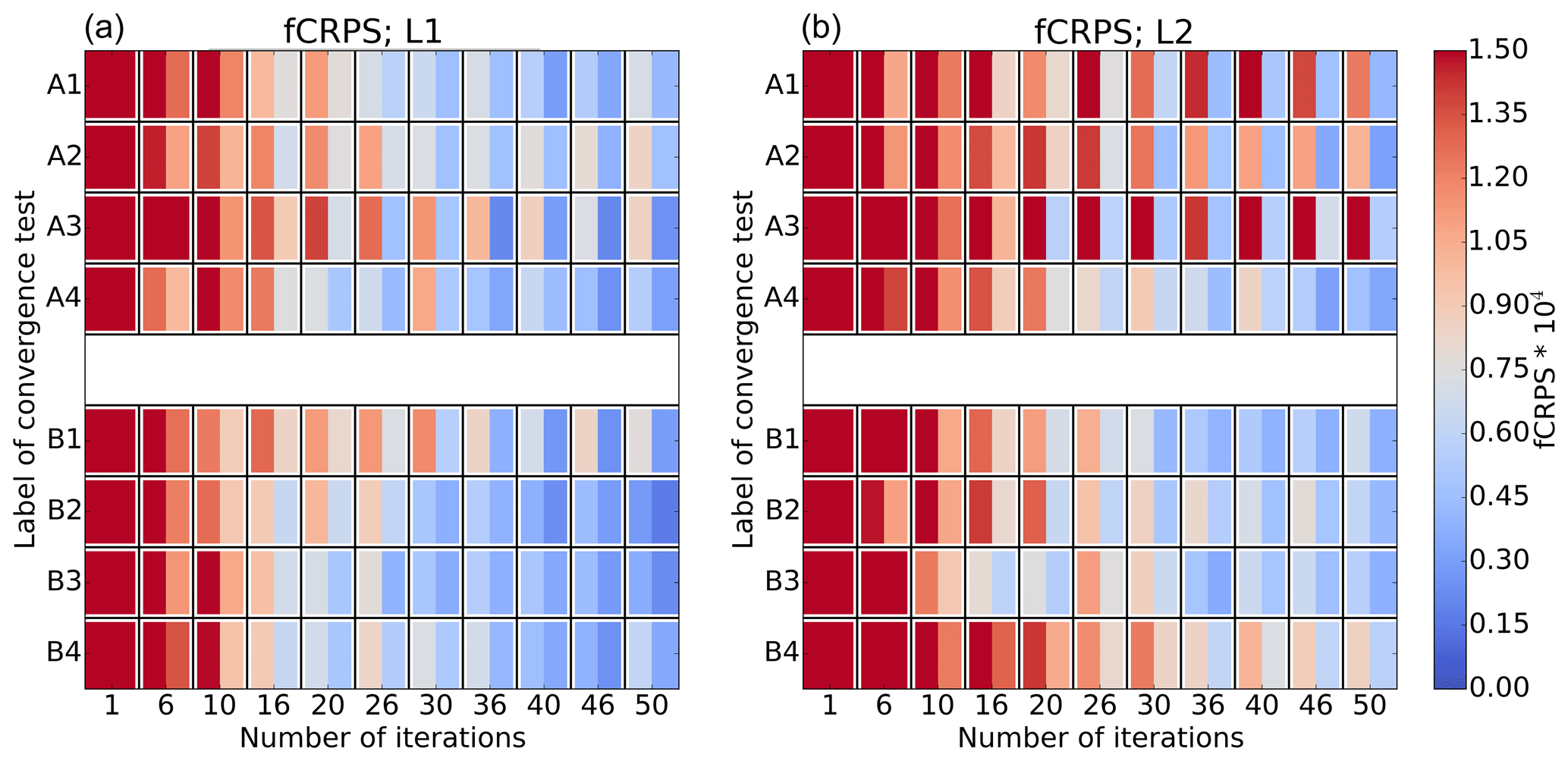
Figure 5Evolution of θ2 in repeated convergence tests with two selected forecast range – ensemble size combinations highlighted in Fig. 3. The level of complexity is (a) L1 and (b) L2. Tests A1 to A4 have been run with forecast range of 48 h and ensemble size of 20 members, and tests B1 to B4 with 24 h and 26 members. EPPES was used as an optimiser in these examples. Components of fCRPS have been calculated using Eqs. (3) and (4).
We recommend using such a setup that is the most likely to yield reliable parameter convergence. At least in our case, the optimal setup of 24 h forecasts and about 20 member ensembles is also the most reliable setup. Also, using only initial condition perturbations (L1) besides the parameter perturbations leads to more reliable convergence than initial condition plus stochastic model perturbations (L2).
4.5 Potential pitfalls
First, during the convergence tests, we noticed that some parameters tend to converge to some off-default values. As an example, the two most used parameters (θ1 and θ2) tend to converge to slightly different values depending on the forecast range used. θ2 tends to converge to a value smaller (larger) value than the default value when forecasts longer (shorter) than 24 h are used. The opposite is true for θ1. However, at least θ2 tends to converge in one-parameter convergence tests in the similar way to that in the two-parameter tests. The behaviour of the parameters is illustrated in Fig. 6, which shows the final mean values for θ1 (Fig. 6a) and for θ2 (Fig. 6b). Convergence of θ2 seems to depend very strongly on the forecast range used in the convergence tests. We now examine the cost functions for two sets of 6 h to 6 d ensemble forecasts: one using the default parameters and one using parameters obtained from the optimisation (Fig. 6). Both sets of ensemble forecasts were compared to respective control forecasts with ΔEm. The tests were repeated with only initial condition perturbations active and with initial condition plus stochastic model perturbations active. Results show that globally optimal parameter values are different from their respective default values even though the default model is used as reference. It is indeed possible to obtain lower cost function values with some off-default parameter values than with the default parameter values. This means that the peculiar dependence is not caused by any deficiencies in the cost function or optimisation algorithms. However, convergence tests and fully realistic tuning are so different that we are unsure about whether this dependency even exists at all in fully realistic tuning. Even if the dependency exists, it is unclear whether it hinders tuning after all.
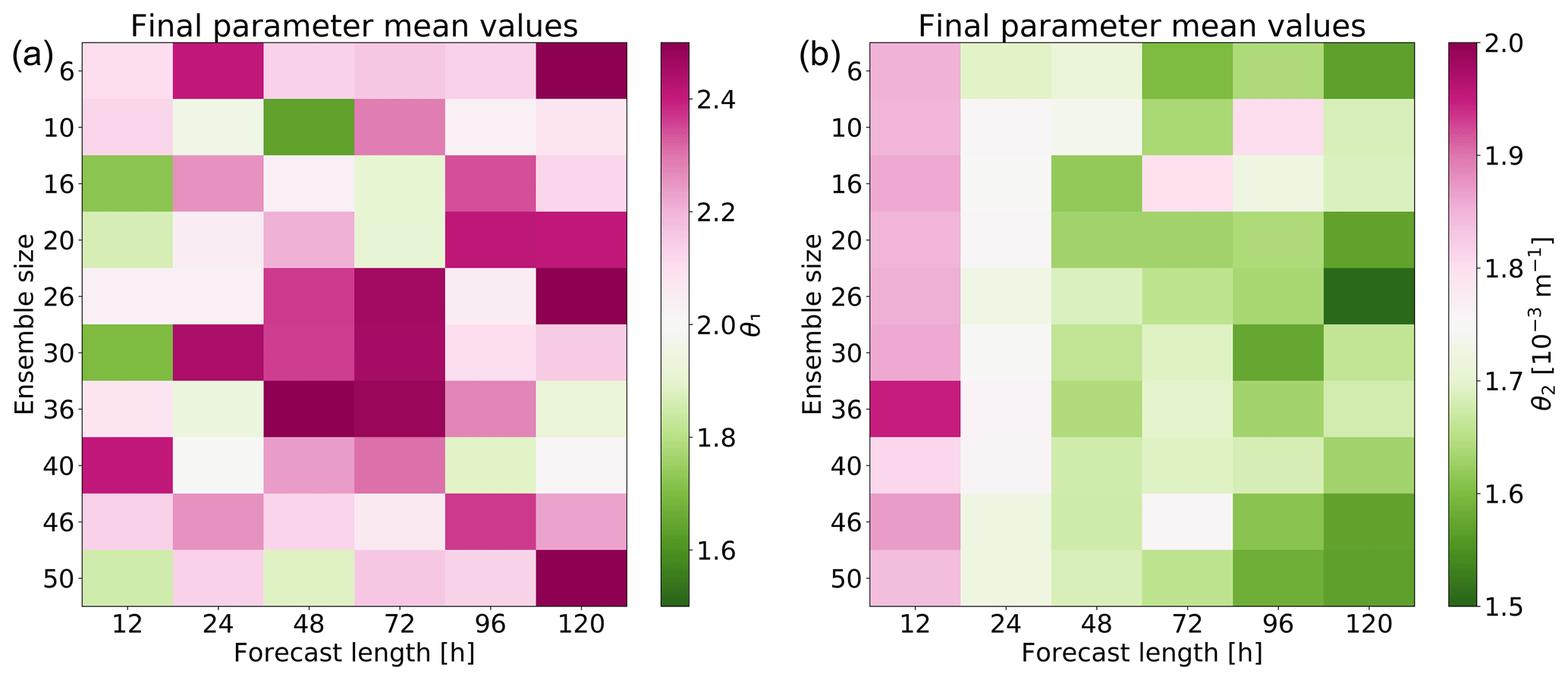
Figure 6Mean values of the parameter distributions proposed by EPPES at the end of the convergence tests: (a) θ1 and (b) θ2. Purple (green) colour means that the final mean values are larger (smaller) than the default value.
A potential pitfall might emerge if there is a need to do algorithmic tuning with ensembles of very different sizes. At least the two algorithms, EPPES and DE, are difficult to set up so that they would work satisfactorily regardless of the ensemble size. If the algorithms produce good convergence with small ensembles of approximately five members, the parameter convergence is very slow with medium-sized and large ensembles, or the parameters may even diverge. Vice versa, if the algorithms work well with medium-sized and large ensembles, they tend to be unstable with small ensembles.
At least two potential pitfalls are related to bad initialisation of tuning exercises. The first pitfall is that convergence of EPPES suffers from too-large initial parameter offsets, while DE is very robust. For example, in an extreme convergence test, where parameter offset is an order of magnitude, convergence of EPPES may stop while DE suffers much less. The second pitfall may be encountered if the initial uncertainty of some parameter is too small with respect to the initial offset, which makes convergence to some local optimum likely. Both algorithms show that in such a case, the badly initialised parameter remains practically unchanged, while the other parameters appear to compensate the error.
We do not recommend completely blind algorithmic tuning. The parameter offset should not be excessively large, and the initial parameter offset and uncertainty should be well proportioned. We also recommend paying attention to selection of the tuning algorithm. In the case of tuning very uncertain parameters, we recommend using robust algorithms, which do not suffer from large parameter offset.
4.6 A recipe for successful tuning
Our recipe for economic and efficient tuning is summarised below:
-
level 1 of complexity (at least initial condition perturbations, possibly also stochastic model perturbations);
-
a comprehensive measure as a cost function (ΔEm in our case);
-
a relatively short forecast range (24 h in our case); and
-
a relatively small ensemble size (20 in our case).
Here, we put the recipe into test with more demanding convergence tests with EPPES. We run four five-parameter tests with TL159, two five-parameter tests with TL399 and one eight-parameter test with TL159 resolution. The parameters in the five-parameter tests are the same as those in the L3 convergence tests. In the eight-parameter test, there are three additional parameters from the convection scheme (see Table 1). The parameters are initialised randomly with an either 10 % too-large or too-small value and large uncertainty. The set of initial conditions is the same as before, meaning 52 iterations.
We discuss all the four TL159 and the two TL399 convergence tests at once, meaning there are a total of 30 converge cases to be discussed (six experiments all involving five parameters). In these six tests, the parameter values converge towards the default values during the convergence tests in 20 out of 30 cases. θ1 converges to an off-default value in four of the cases as does θ3. θ4 converges to an off-default value twice. Furthermore, θ2 tends to converge to a slightly smaller value, and θ1, θ4 and θ5 to slightly larger value than their respective default values. In 25 out of 30 cases, the final parameter value and the default value are both within 2 standard deviations of each other, and hence the default value is inside the parameter distribution proposed by EPPES. In the remaining five cases, the remaining parameter offset is slightly more than 2 standard deviations. These five cases distribute so that each parameter ends up outside of a distance of 2 standard deviations to the default value for one time. In all 30 cases, the uncertainty of the parameter value decreases during the convergence tests meaning that the parameters do converge even though in some cases they converge to some off-default values.
The results of the eight-parameter convergence test are presented in Fig. 7. It shows convergence of the eight parameters in normalised form, and the text boxes in each panel indicate the remaining parameter offset after 52 iterations. All parameters converge towards their default values. In the case of θ5, the default value is outside of the uncertainty range. Additional dimensionality seems to slow down the convergence only a little, which definitely encourages to use algorithmic tuning methods for large parameter sets.
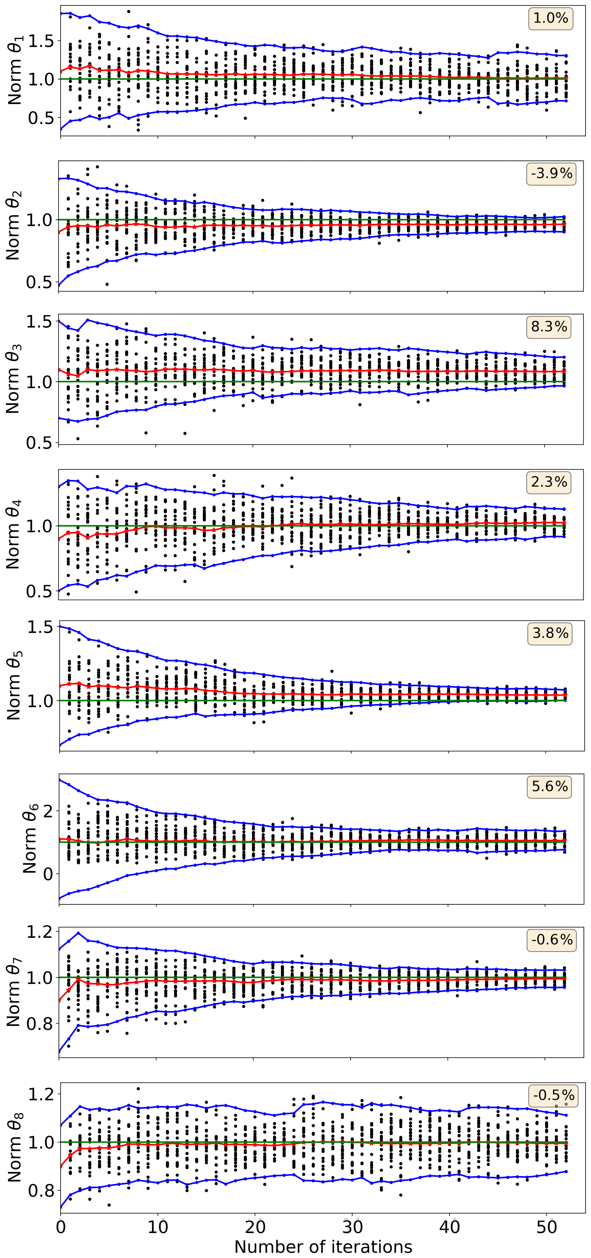
Figure 7Progress of the convergence in the eight-parameter test. The parameter values and uncertainties have been normalised with their default values. Black dots show sampled parameter values, the red line with stars shows parameter mean value, blue lines with dots show mean value ±2 standard deviations, and the green line shows the default parameter value that is 1.0 due to the normalisation. The text boxes indicate the remaining parameter offset, which is the relative distance between the final parameter mean value and the default value. Initial parameter offset is randomly ±10 %.
The choice of the cost function is an essential part of the tuning problem. In order to illustrate the importance of choosing a suitable cost function, we intentionally chose two radically different cost functions: the root mean squared error of geopotential at 850 hPa and the moist total energy norm. The former was, as expected, a bad choice, whereas the latter was a clearly more suitable choice. However, the moist total energy norm was not a perfect choice due to the properties of the tunable parameters. Parameters θ1 and θ2 are not equally sensitive to the components of the moist total energy norm. θ1, which is related to the shallow convection, is active only in the lowest 200 hPa layer of the model atmosphere. θ1 mainly affects how specific humidity is distributed in the layer. Therefore, contribution of θ1 comes almost only from lower tropospheric specific humidity. θ2 controls deep convection so it has direct impact on wind, temperature and specific humidity throughout the model troposphere. Therefore, contribution of θ2 to the cost function dominates, which may in some cases decrease the overall sensitivity of the moist total energy norm when estimating the two parameters simultaneously. An option would be to use multiple cost functions, having one dedicated for each tunable parameter. However, this could lead to a question of scaling: would each cost function have equal weight or are some of the cost functions considered more important? At the moment, we do not have a definitive answer for this.
In our study, we aimed at finding an optimal setup for convergence tests by studying different combinations of forecast range and ensemble size. Using an ensemble of 20 members and a forecast range of 24 h gave the best results. When the ensemble size is too small, the sample size will also be small, which could lead to the case of not having a representative sample. A forecast range of 24 h seems optimal. When the forecast range is shorter, θ1 tends to converge to smaller values and θ2 to larger values than the default parameter value, whereas a longer forecast leads to θ1 converging to larger value and θ2 to smaller value than the default value. The question of whether the parameter values depend on the forecast range is profound. The entire forecast range could also be considered but may lead to similar scaling issues (e.g. Ollinaho et al., 2013) as when using multiple cost functions.
The two optimisers used in this study, EPPES and DE, have different properties. EPPES converges more slowly and estimates the covariance matrix of the parameters, whereas DE gives faster but less steady convergence. The optimisers could therefore be used at different stages of the optimisation: first, DE could be used as a coarse tuner finding the approximate direction, and then EPPES could be used to fine tune the results. This type of tuning process would be of most use when the parameters are known poorly a priori.
Local minima of the cost function are potential problems. According to our observations, convergence to a local minimum may occur if the initialisation of the parameter values is bad. A large initial distance from the optimal value combined with a too-small initial uncertainty range might lead to a case where the cost function becomes locally minimised, and the algorithm gets stuck exploring parameter values from around this local minimum. Other parameters may compensate the error, and the cost function becomes locally minimised. When the parameters are initialised appropriately and initial condition perturbations are active, problems of this sort are less likely.
We compared the perturbed forecasts against the control forecast run with default parameters. In this case, one would expect that forecasts with default parameters would result in minimum cost function, but this turned out not to be the case. This leads us to the question of whether changing the values of the model parameters affects properties of the ensemble, such as its spread. In a well-tuned ensemble prediction system, not only should the model be as good as possible (i.e. having optimal parameter values) but the relationship between the spread of the ensemble and the ensemble mean skill should be in balance. We leave this question open for future studies.
In this paper, we have studied the convergence properties of two algorithms used for tuning model physics parameters in a numerical weather prediction model. The tuning process is a computationally demanding task and using an optimal experimental setup would minimise the amount of computational resources required.
In our experiments, we studied two different tuning algorithms and how the convergence properties were affected by (1) the choice of cost function, (2) forecast range, (3) ensemble size and (4) the complexity of the model setup (perturbations of initial conditions and stochastic physics turned on or off). In our case, we focused on tuning two parameters of the convection scheme of the OpenIFS model. The model resolution in these tests was T159 (about 125 km).
Our goal was to find an optimal setup of forecast range and ensemble size with the highest likelihood for fast and reliable convergence, hence minimising the amount of computations. We ran many convergence tests with different experimental setups, calculated the moist total energy norm between the forecasts with perturbed parameters and the control forecast having default parameters values, calculated a fair verification metric (fCRPS) and finally compared the experiments against each other. The optimal setup in our experiments was an ensemble of 20 members and a forecast range of 24 h.
We tested the optimal setup for a more complex optimisational task: tuning five and eight parameters at once. In these experiments, the ensemble had 20 members, the forecast range was 24 h, and the algorithm was run for 52 iterations. Such an experiment would be the same as running a single 1040 d forecast consuming roughly 400 core hours for TL159 model resolution and 4200 core hours for TL399 model resolution on Intel Haswell computation nodes. These experiments showed that the convergence of most of the parameters was good.
Finally, we conclude our study by answering the question of whether algorithmic tuning (of model physics parameters) could be trusted: the answer is yes when used with care.
A1 Experimental details of EPPES
EPPES needs four hyperparameters: μ, Σ, W and n. The former two describe the initial guess for the distribution of the parameters that are to be estimated, whereas the latter two describe how accurate the initial guess is.
Let be the closure parameters. In EPPES, the prior guess is that the closure parameter follows a Gaussian distribution , where μ is the mean vector of θ and Σ the covariance matrix.
Details of initialisation of the parameter distribution are listed in Table A1 and other settings of EPPES are summarised in Table A2. The mean values are always multiplied with 0.9 or 1.1 in the initialisation of the convergence tests.
Table A1Initial values of the convection parameters for EPPES.
A2 Experimental details of DE
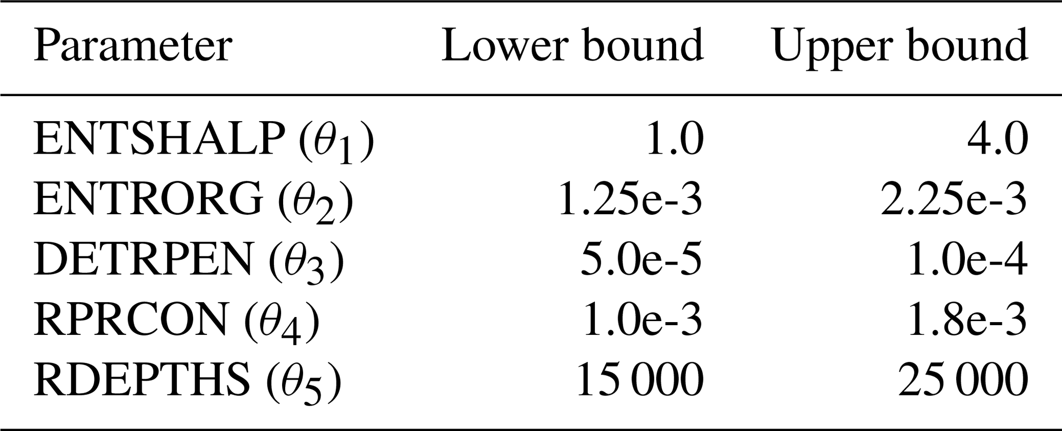
DE requires the boundaries for the parameter search domain to be specified. DE does not explicitly limit any searching directions by default, but some constraints can be specified in order to avoid unfeasible parameter values. In our case, we are targeting only non-negative values.
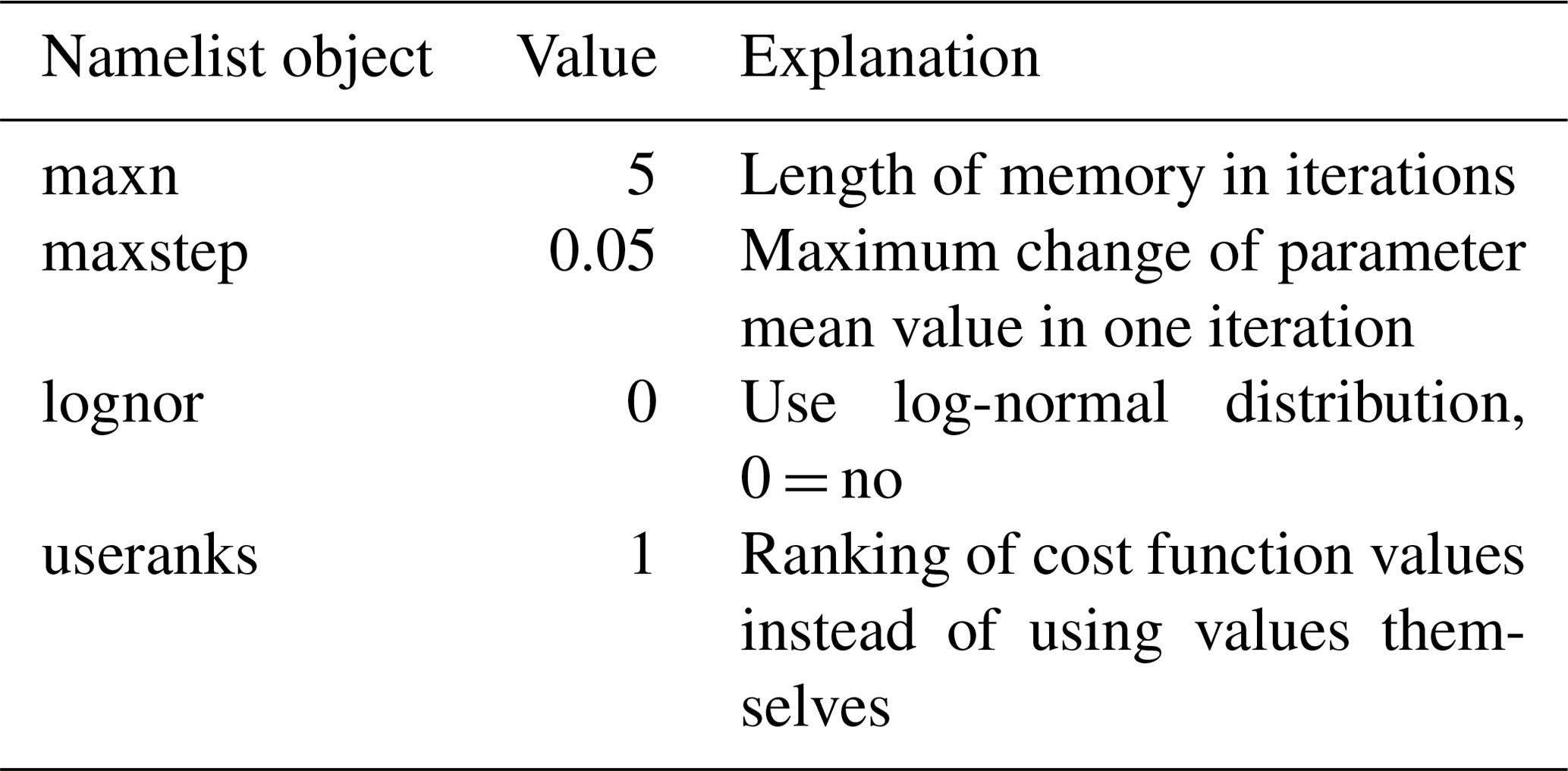
The initial search domain is specified in Table A3 and other settings written in the namelist file are summarised in Table A4.
The recalculation step is employed every fifth iteration; it substitutes all usual DE steps (mutation, crossover, selection) and just computes/updates the value of the cost function in the current environment for the elements already in the population.

The basic version of OpenEPS is available under Apache licence version 2.0, January 2004 on Zenodo (https://doi.org/10.5281/zenodo.3759127; Ollinaho, 2020). The amended version of OpenEPS, which was used in the convergence tests, is also available under Apache licence version 2.0, January 2004 on Zenodo (https://doi.org/10.5281/zenodo.3757601; Ollinaho and Tuppi, 2020). The amended version contains various modifications such as setup scripts for EPPES and DE, scripts for calculating cost function values and scripts for processing and plotting output of convergence tests. The latest development versions of OpenEPS are available on GitHub (https://github.com/pirkkao/OpenEPS, last access: 19 November 2020 and https://github.com/laurituppi/OpenEPS, last access: 19 November 2020). The licence for using the OpenIFS NWP model can be requested from ECMWF user support (openifs-support@ecmwf.int). EPPES is available under MIT licence on Zenodo (https://doi.org/10.5281/zenodo.3757580; Laine, 2020), and DE is available upon request from vladimir.shemyakin@lut.fi. The initial conditions used in the convergence tests belong to a larger data set. Availability of the data set will be described in Ollinaho et al. (2020). We want to emphasise that reproducing the results does not require using exactly the same initial conditions as in this paper and any OpenIFS ensemble initial conditions can be used. Output data of the convergence tests are not archived since they can be easily reproduced.
LT and PO designed the convergence tests, and LT carried them out. PO provided initial conditions and OpenEPS with comprehensive user support. VS provided hands-on assistance in using DE in the convergence tests. LT prepared the manuscript with contributions and comments from all co-authors. HJ and ME helped with clear formulation of the text. HJ supervised the experimentation and production of the manuscript.
The authors declare that they have no conflict of interest.
The authors are grateful to CSC-IT Center for Science, Finland, for providing computational resources, and Juha Lento at CSC-IT for user support with the supercomputers. We thank Olle Räty at Finnish Meteorological Institute for assisting in graphical design of Fig. 3. We are also thankful to Marko Laine at Finnish Meteorological Institute for the insightful discussions about evaluation of convergence tests and user support for EPPES. The figures have been plotted with the help of the Python Matplotlib library (Hunter, 2007). CDO (Schulzweida, 2019) was used for post-processing the output of OpenIFS. We would like to acknowledge the funding from the Academy of Finland (grant nos. 333034 and 316939), the Vilho, Yrjö and Kalle Väisälä Foundation of the Finnish Academy of Science and Letters and funding and support from Doctoral Programme in Atmospheric Sciences of University of Helsinki. Finally, we would like to thank Peter Düben and Joakim Kjellsson for their valuable comments for improving the manuscript further.
Funding was provided by the Academy of Finland (grant nos. 333034 and 316939), the Vilho, Yrjö and Kalle Väisälä Foundation of the Finnish Academy of Science and Letters, and Doctoral Programme in Atmospheric Sciences of University of Helsinki.
Open-access funding was provided by the Helsinki University Library.
This paper was edited by Simone Marras and reviewed by Peter Düben and Joakim Kjellsson.
Annan, J. D., Lunt, D. J., Hargreaves, J. C., and Valdes, P. J.: Parameter estimation in an atmospheric GCM using the Ensemble Kalman Filter, Nonlin. Processes Geophys., 12, 363–371, https://doi.org/10.5194/npg-12-363-2005, 2005. a
Bechtold, P., Köhler, M., Jung, T., Doblas-Reyes, F., Leutbecher, M., Rodwell, M. J., Vitart, F., and Balsamo, G.: Advances in simulating atmospheric variability with the ECMWF model: From synoptic to decadal time-scales, Q. J. Roy. Meteor. Soc., 134, 1337–1351, https://doi.org/10.1002/qj.289, 2008. a
Chakraborty, U. K.: Advances in Differential Evolution, vol. 143, Springer, Verlag, https://doi.org/10.1007/978-3-540-68830-3, 2008. a, b, c
ECMWF: IFS documentation. Part IV: Physical processes, CY40R1, available at: https://www.ecmwf.int/sites/default/files/elibrary/2014/9204-part-iv-physical-processes.pdf (last access: 19 November 2020), 2014. a, b
ECMWF: Changes in ECMWF model, available at: https://www.ecmwf.int/en/forecasts/documentation-and-support/changes-ecmwf-model (last access: 19 November 2020), 2019. a
Ehrendorfer, M., Errico, R. M., and Raeder, K. D.: Singular-Vector Perturbation Growth in a Primitive Equation Model with Moist Physics, J. Atmos. Sci., 56, 1627–1648, https://doi.org/10.1175/1520-0469(1999)056<1627:SVPGIA>2.0.CO;2, 1999. a
Feoktistov, V.: Differntial Evolution: In Search of Solutions, Springer Science, 2006. a, b
Ferro, C. A. T., Richardson, D. S., and Weigel, A. P.: On the effect of ensemble size on the discrete and continuous ranked probability scores, Meteorol. Appl., 15, 19–24, https://doi.org/10.1002/met.45, 2008. a
Goldberg, D. E.: Genetic Algorithms in Search, Optimization and Machine Learning, Addison-Wesley, 1989. a
Hourdin, F., Mauritsen, T., Gettelman, A., Golaz, J., Balaji, V., Duan, Q., Folini, D., Ji, D., Klocke, D., Qian, Y., Rauser, F., Rio, C., Tomassini, L., Watanabe, M., and Williamson, D.: The Art and Science of Climate Model Tuning, B. Am. Meteorol. Soc., 98, 589–602, https://doi.org/10.1175/BAMS-D-15-00135.1, 2017. a
Hunter, J. D.: Matplotlib: A 2D graphics environment, Comput. Sci. Eng., 9, 90–95, https://doi.org/10.1109/MCSE.2007.55, 2007. a
Ingber, L.: Very fast simulated re-annealing, Math. Comput. Model., 12, 967–973, https://doi.org/10.1016/0895-7177(89)90202-1, 1989. a
Jakob, C.: Accelerating Progress in Global Atmospheric Model Development through Improved Parameterizations: Challenges, Opportunities, and Strategies, B. Am. Meteorol. Soc., 91, 869–876, https://doi.org/10.1175/2009BAMS2898.1, 2010. a
Järvinen, H., Laine, M., Solonen, A., and Haario, H.: Ensemble prediction and parameter estimation system: the concept, Q. J. Roy. Meteorol. Soc., 138, 281–288, https://doi.org/10.1002/qj.923, 2012. a, b
Kennedy, J.: Particle Swarm Optimization, Springer US, Boston, MA, 760–766, https://doi.org/10.1007/978-0-387-30164-8_630, 2010. a
Kivman, G. A.: Sequential parameter estimation for stochastic systems, Nonlin. Processes Geophys., 10, 253–259, https://doi.org/10.5194/npg-10-253-2003, 2003. a
Laine, M.: mjlaine/eppes: initial release (Version v1.0), Zenodo, https://doi.org/10.5281/zenodo.375758, 2020. a
Laine, M., Solonen, A., Haario, H., and Järvinen, H.: Ensemble prediction and parameter estimation system: the method, Q. J. Roy. Meteor. Soc., 138, 289–297, https://doi.org/10.1002/qj.922, 2012. a, b
Leutbecher, M.: Ensemble size: How suboptimal is less than infinity?, Q. J. Roy. Meteor. Soc., 145, 107–128, https://doi.org/10.1002/qj.3387, 2018. a, b, c
Mauritsen, T., Stevens, B., Roeckner, E., Crueger, T., Esch, M., Giorgetta, M., Haak, H., Jungclaus, J., Klocke, D., Matei, D., Mikolajewicz, U., Notz, D., Pincus, R., Schmidt, H., and Tomassini, L.: Tuning the climate of a global model, J. Adv. Model. Earth Sy., 4, M00A01, https://doi.org/10.1029/2012MS000154, 2012. a
Ollinaho, P.: pirkkao/OpenEPS: Initial release (Version v0.952), Zenodo, https://doi.org/10.5281/zenodo.3759127, 2020. a
Ollinaho, P. and Tuppi, L.: laurituppi/OpenEPS: OpenEPS for convergence testing (Version v1.0), Zenodo, https://doi.org/10.5281/zenodo.3757601, 2020. a
Ollinaho, P., Laine, M., Solonen, A., Haario, H., and Järvinen, H.: NWP model forecast skill optimization via closure parameter variations, Q. J. Roy. Meteor. Soc., 139, 1520–1532, https://doi.org/10.1002/qj.2044, 2013. a
Ollinaho, P., Järvinen, H., Bauer, P., Laine, M., Bechtold, P., Susiluoto, J., and Haario, H.: Optimization of NWP model closure parameters using total energy norm of forecast error as a target, Geosci. Model Dev., 7, 1889–1900, https://doi.org/10.5194/gmd-7-1889-2014, 2014. a, b, c, d
Ollinaho, P., Lock, S.-J., Leutbecher, M., Bechtold, P., Beljaars, A., Bozzo, A., Forbes, R. M., Haiden, T., Hogan, R. J., and Sandu, I.: Towards process-level representation of model uncertainties: stochastically perturbed parametrizations in the ECMWF ensemble, Q. J. Roy. Meteor. Soc., 143, 408–422, https://doi.org/10.1002/qj.2931, 2017. a
Ollinaho, P., Carver, G. D., Lang, S. T. K., Tuppi, L., Ekblom, M., and Järvinen, H.: Ensemble prediction using a new dataset of ECMWF initial states – OpenEnsemble 1.0, Geosci. Model Dev. Discuss., https://doi.org/10.5194/gmd-2020-292, in review, 2020. a, b
Palmer, T., Buizza, R., Doblas-Reyes, F., Jung, T., Leutbecher, M., Shutts, G., Steinheimer, M., and Weisheimer, A.: Stochastic parametrization and model uncertainty, ECMWF Technical Memoranda, 598, 1–42, 2009. a
Pulido, M., Tandeo, P., Bocquet, M., Carrassi, A., and Lucini, M.: Stochastic parameterization identification using ensemble Kalman filtering combined with maximum likelihood methods, Tellus A, 70, 1–17, https://doi.org/10.1080/16000870.2018.1442099, 2018. a
Qing, A.: Differential Evolution: Fundamentals and Applications in Electrical Engineering, Wiley, https://doi.org/10.1002/9780470823941, 2009. a
Schulzweida, U.: CDO User Guide, Zenodo, https://doi.org/10.5281/zenodo.2558193, 2019. a
Shemyakin, V. and Haario, H.: Online identification of large-scale chaotic system, Nonlinear Dynam., 93, 961–975, https://doi.org/10.1007/s11071-018-4239-5, 2018. a, b
Storn, R. and Price, K.: Differential Evolution – A Simple and Efficient Heuristic for global Optimization over Continuous Spaces, J. Global Optim., 11, 341–359, https://doi.org/10.1023/A:1008202821328, 1997. a, b, c