COSIPY v1.3 – an open-source coupled snowpack and ice surface energy and mass balance model

Glacier changes are a vivid example of how environmental systems react to a changing climate. Distributed surface mass balance models, which translate the meteorological conditions on glaciers into local melting rates, help to attribute and detect glacier mass and volume responses to changes in the climate drivers. A well-calibrated model is a suitable test bed for sensitivity, detection, and attribution analyses for many scientific applications and often serves as a tool for quantifying the inherent uncertainties. Here, we present the open-source COupled Snowpack and Ice surface energy and mass balance model in PYthon (COSIPY), which provides a flexible and user-friendly framework for modeling distributed snow and glacier mass changes. The model has a modular structure so that the exchange of routines or parameterizations of physical processes is possible with little effort for the user. The framework consists of a computational kernel, which forms the runtime environment and takes care of the initialization, the input–output routines, and the parallelization, as well as the grid and data structures. This structure offers maximum flexibility without having to worry about the internal numerical flow. The adaptive subsurface scheme allows an efficient and fast calculation of the otherwise computationally demanding fundamental equations. The surface energy balance scheme uses established standard parameterizations for radiation as well as for the energy exchange between atmosphere and surface. The schemes are coupled by solving both surface energy balance and subsurface fluxes iteratively such that consistent surface skin temperature is returned at the interface. COSIPY uses a one-dimensional approach limited to the vertical fluxes of energy and matter but neglects any lateral processes. Accordingly, the model can be easily set up in parallel computational environments for calculating both energy balance and climatic surface mass balance of glacier surfaces based on flexible horizontal grids and with varying temporal resolution. The model is made available on a freely accessible site and can be used for non-profit purposes. Scientists are encouraged to actively participate in the extension and improvement of the model code.

1 Introduction

Glacier variations are of great interest and relevance in many scientific issues and application such as climate sciences, water resources management, and tourism. In order to identify the climatic drivers for past, current, and future changes, process understanding, observations, and models of glacier mass change need to be combined appropriately. Schemes that relate the surface mass balance of snow and ice bodies to meteorological forcing data have been set up and applied for many decades (e.g., Anderson, 1968; Kraus, 1975; Anderson, 1976; Kuhn, 1979; Male and Granger, 1981; Kuhn, 1987; Siemer, 1988; Morris, 1989, 1991; Munro, 1991). Studies have shown that the synthesis of this information provides a consistent understanding of the relevant mass and energy fluxes at the glacier–atmosphere interface, which in turn provides the necessary physical foundations to translate micrometeorological conditions on glaciers into local melt rates (e.g., Sauter and Galos, 2016; Wagnon et al., 1999; Oerlemans, 2001; Mölg and Hardy, 2004; Obleitner and Lehning, 2004; Van Den Broeke et al., 2006; Reijmer and Hock, 2008; Mölg et al., 2008; Nicholson et al., 2013). Distributed mass balance models combine the local melt information with glacier-wide surface mass change information and thus offer the possibility to attribute and detect glacier mass and volume responses to changes in the climatic forcings (e.g., Klok and Oerlemans, 2002; Hock and Holmgren, 2005; Mölg et al., 2009; Sicart et al., 2011; Cogley et al., 2011). Although the accumulation and redistribution of snow are still deficient (e.g., Sauter et al., 2013), when coupled with atmospheric models, such models have the potential to simulate present and future glacier evolution or to serve as a useful tool for monitoring climatic glacier mass change (Machguth et al., 2006). A well-calibrated model is a suitable platform for sensitivity, detection, and attribution analyses as well as a tool for the quantification of inherent uncertainties (e.g., Mölg et al., 2014; Maussion et al., 2015; Rye et al., 2012; Mölg et al., 2012; Sauter and Obleitner, 2015; Galos et al., 2017; van Pelt et al., 2012; Østby et al., 2017).

Over recent decades, several distributed mass balance models of varying complexity have been developed and successfully applied to different glacier systems and climate regimes. The models range from simple degree-day models (e.g., Radić and Hock, 2006; Schuler et al., 2005) to intermediate models (e.g., Machguth et al., 2009) and complex snow cover and glacier-resolving physical models (e.g., Bartelt and Lehning, 2002; Vionnet et al., 2012; Hock and Holmgren, 2005; Klok and Oerlemans, 2002; Sicart et al., 2011; Weidemann et al., 2018; Huintjes et al., 2015b; Mölg et al., 2009; Michlmayr et al., 2008; van Pelt et al., 2012). The latter model class is usually based on the same fundamental physical principles but differs in the parameterization schemes and implementation techniques. Different research groups have their own in-house solutions which are often extended and modified for specific scientific questions and studies. The fact that often several subversions of the same model exist, with some of them not being freely available, makes it difficult for users to having access to up-to-date software. Ideally, a platform should (i) be continuously maintained, (ii) provide newly developed parameterizations, (iii) compile different model subversions developed for specific research needs, (iv) be easily extensible, and (v) be well documented and readable.

Here, we present an open-source COupled Snowpack and Ice surface energy and mass balance model in PYthon (COSIPY) designed to meet these requirements. The structure is based on the predecessor model COSIMA (COupled Snowpack and Ice surface energy and MAss balance model; Huintjes et al., 2015b). COSIPY provides a lean, flexible, and user-friendly framework for modeling distributed snow and glacier mass changes. The framework consists of a computational core that forms the runtime environment and handles initialization, input–output (IO) routines, parallelization, and the grid and data structures. In most cases, the runtime environment does not require any changes by the user. To increase the user friendliness, additional features are available, such as a restart option for operational applications and automatic comparison between simulation and ablation stakes. These features will be further refined in the future. Physical processes and parameterizations are handled separately by modules. The modules can be easily modified or extended to meet the needs of the end user. This structure provides maximum flexibility without worrying about internal numerical issues. The model is completely based on open-source libraries and is provided on a freely accessible Git repository (https://github.com/cryotools/cosipy, last access: 11 November 2020) for non-profit purpose. Scientists can actively participate in extending and improving the model code. Changes to the code are automatically tested with Travis CI (http://www.travis-ci.org, last access: 11 November 2020) when uploaded to the repository. It is planned to publish updates in regular intervals. To make working with COSIPY easier, a community platform (https://cosipy.slack.com, last access: 11 November 2020) has been set up in addition to a detailed “Read the Docs” documentation (https://cosipy.readthedocs.io/en/latest, last access: 11 November 2020), allowing users and developers to exchange experiences, report bugs, and communicate needs. In this work, we describe the physical basics and parameterizations, and outline the numerical implementation of the COSIPY model (version 1.3) (https://zenodo.org/record/3902191, Sauter and Arndt, 2020a). Section 2 gives an overview of the model concept, followed by the description of the modules (Sect. 3). The model architecture and the input–output are explained in Sect. 4. Section 5 shows different applications of the model. The code availability section documents the code availability and software requirements.

2 Model concept

2.1 Fundamental equations

COSIPY is a multi-layered process resolving energy and mass balance model for the simulation of past, current, and future glacier changes. The model is based on the concept of energy and mass conservation. The snow/ice layers are described by the volumetric fraction of ice θ_i, liquid water content θ_w, and air porosity θ_a. Continuity constraints require that

$$\begin{array}{}\text{(1)}& {\mathit{\theta }}_{\mathrm{i}}+{\mathit{\theta }}_{\mathrm{w}}+{\mathit{\theta }}_{\mathrm{a}}=\mathrm{1}.\end{array}$$

The inherent properties, such as snow density ρ_s or specific heat of snow c_s, follow from the volumetrically weighted properties of the constitutes. For example, snow density is related by

$$\begin{array}{}\text{(2)}& {\mathit{\rho }}_{\mathrm{s}}={\mathit{\theta }}_{\mathrm{i}}\cdot {\mathit{\rho }}_{\mathrm{i}}+{\mathit{\theta }}_{\mathrm{w}}\cdot {\mathit{\rho }}_{\mathrm{w}}+{\mathit{\theta }}_{\mathrm{a}}\cdot {\mathit{\rho }}_{\mathrm{a}},\end{array}$$

where ρ_i is the ice density, ρ_w the water density, and ρ_a the air density (Bartelt and Lehning, 2002). Exchange processes at the surface, the energy release and consumption through phase changes, control the vertical temperature distribution within the snow and ice layers. The energy balance also includes incoming shortwave radiation absorption and the sublimation or deposition of water vapor. Assuming the vertical temperature profile is given by T_s(z,t), where z is the depth, the energy conservation can be represented by

$$\begin{array}{}\text{(3)}& \begin{array}{rl}& {\mathit{\rho }}_{\mathrm{s}}(z,t)c_{\mathrm{s}}(\mathit{\theta },z,t){\displaystyle \frac{\partial T_{\mathrm{s}}(z,t)}{\partial t}}-k_{\mathrm{s}}(\mathit{\theta },z,t){\displaystyle \frac{{\partial }^{\mathrm{2}}{T}_{\mathrm{s}}(z,t)}{\partial z^{\mathrm{2}}}}\\ & =Q_{\mathrm{p}}(z,t)+Q_{\mathrm{r}}(z,t),\end{array}\end{array}$$

where $c_{\mathrm{s}}=c_{\mathrm{i}}{\mathit{\theta }}_{\mathrm{i}}+c_{\mathrm{w}}$ θ_w+c_pθ_a and $k_{\mathrm{s}}=k_{\mathrm{i}}{\mathit{\theta }}_{\mathrm{i}}+k_{\mathrm{w}}{\mathit{\theta }}_{\mathrm{w}}+k_{\mathrm{a}}{\mathit{\theta }}_{\mathrm{a}}$ are the volume-specific bulk heat capacity and bulk thermal conductivity of the snow cover (Bartelt and Lehning, 2002). Alongside the volume-specific heat capacity, COSIPY also offers the option of using empirical form $k_{\mathrm{s}}=\mathrm{0.021}+\mathrm{2.5}({\mathit{\rho }}_{\mathrm{s}}/\mathrm{1000.0}{)}^{\mathrm{2}}$ (Huintjes et al., 2015a). The first term on the right-hand side (Q_p) is the volumetric energy sink or source by melting and meltwater refreezing. The second term (Q_r) is the volumetric energy surplus by the absorption of shortwave radiation (see Eq. 13).

The exchange processes at the snow/ice–atmosphere interface control the surface temperature $T_{\mathrm{s}}(z=\mathrm{0},t)$ at an infinitesimal skin layer. From the energy conservation follows

$$\begin{array}{}\text{(4)}& k_{\mathrm{s}}(\mathit{\theta },z=\mathrm{0},t){\displaystyle \frac{\partial T_{\mathrm{s}}(z=\mathrm{0},t)}{\partial z}}=q_{\mathrm{sw}}+q_{\mathrm{lw}}+q_{\mathrm{sh}}+q_{\mathrm{lh}}+q_{\mathrm{rr}},\end{array}$$

where q_sw is the net-shortwave radiation energy, q_lw is the net-longwave radiation energy, q_sh is the sensible heat flux, q_lh is the latent heat flux, and q_rr is the heat flux from rain. To solve Eq. (4) for $T_{\mathrm{s}}(z=\mathrm{0},t)$, the fluxes on the right-hand side must be parameterized (see Sect. 3). The parameterization results in a nonlinear equation which is solved iteratively. The left side of Eq. (4) provides the upper Neumann boundary condition (prescribed gradient) for Eq. (3). At the bottom of the domain, the temperature must be specified (Dirichlet boundary condition) by the user. The melting rates in the snow cover and glacier ice are derived diagnostically from the energy conservation by ensuring that the temperature does not exceed the melting point temperature T_m.

Equation (4) is solved using a limited-memory Broyden–Fletcher–Goldfarb–Shanno (BFGS) algorithm (quasi-Newton method) for bound-constrained minimization (Fletcher, 2000). Equation (3) is then integrated with an implicit second-order central difference scheme (Ferziger and Perić, 2002). The heat sources can warm the snowpack and lead to internal melt processes. In the event that the liquid water content of a layer exceeds its irreducible water content (Coléou and Lesaffre, 1998; Wever et al., 2014),

$$\begin{array}{}\text{(5)}& {\displaystyle }{\mathit{\theta }}_e={\displaystyle }\left\{\begin{array}{ll}\mathrm{0.0264}+\mathrm{0.0099}\frac{(\mathrm{1}-{\mathit{\theta }}_{\mathrm{i}})}{{\mathit{\theta }}_{\mathrm{i}}},& \text{if}{\mathit{\theta }}_{\mathrm{i}}\le \mathrm{0.23}\\ \mathrm{0.08}-\mathrm{0.1023}({\mathit{\theta }}_{\mathrm{i}}-\mathrm{0.03}),& \text{if}\mathrm{0.23}<{\mathit{\theta }}_{\mathrm{i}}\le \mathrm{0.812}\\ \mathrm{0},& \text{if}{\mathit{\theta }}_{\mathrm{i}}>\mathrm{0.812}\end{array}\right.,\end{array}$$

the excess water is drained into the subsequent layer (bucket approach). The liquid water is passed on until it reaches either a layer of ice or the glacier surface where it is considered to be runoff. For this purpose, a threshold value was introduced which defines the transition from snow to ice. If no such layer exists, water is passed on until it reaches the lower limit of the domain and is then considered as runoff. Meltwater refreezing and subsurface melting during percolation change the volumetric ice and water contents. Subsurface melt occurs when energy fluxes, e.g., penetrating shortwave radiation, warm the layer to physically inconsistent temperatures of T_s>T_m. Since physical constraints require that T_s≤T_m, the energy surplus is used to melt the ice matrix. Melt takes place when T_s>T_m and the liquid water content increases by

$$\begin{array}{}\text{(6)}& \mathrm{\Delta }{\mathit{\theta }}_{\mathrm{w}}(z,t)={\displaystyle \frac{c_{\mathrm{i}}(z,t){\mathit{\theta }}_{\mathrm{i}}(z,t){\mathit{\rho }}_{\mathrm{i}}(z,t)\left(T_{\mathrm{s}}\right(z,t)-T_{\mathrm{m}})}{L_{\mathrm{f}}{\mathit{\rho }}_{\mathrm{w}}}},\end{array}$$

where $L_{\mathrm{f}}=\mathrm{3.34}\times {\mathrm{10}}^{\mathrm{5}}$ J Kg⁻¹ is the latent heat of fusion (Bartelt and Lehning, 2002). Mass conservation requires that the mass gain of liquid water content equals the mass loss of the volumetric ice content, so that

$$\begin{array}{}\text{(7)}& \mathrm{\Delta }{\mathit{\theta }}_{\mathrm{i}}(z,t)={\displaystyle \frac{{\mathit{\rho }}_{\mathrm{w}}\mathrm{\Delta }{\mathit{\theta }}_{\mathrm{w}}(z,t)}{{\mathit{\rho }}_{\mathrm{i}}}}.\end{array}$$

The latent energy needed by the phase change is

$$\begin{array}{}\text{(8)}& Q_{\mathrm{p}}(z,t)=L_{\mathrm{f}}\mathrm{\Delta }{\mathit{\theta }}_{\mathrm{i}}(z,t){\mathit{\rho }}_{\mathrm{i}},\end{array}$$

which is an heat sink because Δθ_i(z,t) is positive at melting. The energy used for melting ensures that T_s(z,t) does not rise above T_m. In the event that θ_w>0 and T_s<T_m, refreezing can take place. Changes in volumetric fractions and the release of latent energy due to phase changes are treated equally. As the temperature difference must be negative due to the given constraints, it follows from Eqs. (6), (7), and (8) that Q_p becomes positive and latent heat release warms the layer.

Many of the quantities and fluxes in Eqs. (3) and (4) are not measured directly and have to be derived via corresponding parameterizations. The next section describes the parameterizations implemented in COSIPY v1.3.

2.2 Discretization and computational mesh

To solve the underlying differential equations, the computing domain must be discretized. Since extreme gradients in temperature, density, and liquid water content can develop in the snowpack, COSIPY uses a dynamic, non-equidistant mesh. The mesh consists of so-called nodes that store the properties of the layers (e.g., temperature, density, and liquid water content) and is continuously adjusted during runtime by a re-meshing algorithm; i.e., the number and height of the individual layers vary with time. Currently, two algorithms are implemented: the first is a logarithmic approach, where the layer thicknesses gradually increase with depth by a constant stretching factor. Thus, layers close to the surface have a higher spatial resolution, which is advantageous for the computation of the energy and mass fluxes at the surface. Re-meshing is performed at each time step. This is a fast method but does not resolve sharp layering transitions, as these are smoothed by the algorithm. This approach is only recommended if a detailed resolution of the snow and ice cover is not required. The other algorithm implemented is an adaptive one that assembles layers according to user-defined criteria. It uses density and temperature thresholds to determine when two successive layers are considered similar and when they are not. When both criteria are met, these layers are merged. Basically, the adaptive algorithm runs in three consecutive steps: (1) adding/removing snow/ice at the surface, (2) adjusting the first layer, (3) updating internal layers.

1. In the first step, it is checked whether snow falls or melts away (note that internal layers can also melt). If snow falls on the glacier surface, it will only remain on the surface if it reaches a user-defined minimum snow thickness. Melt is removed from the first layer and all internal layers. After this step, layers can become very small and the thickness of the first layer no longer corresponds to the user-specified constant thickness. Therefore, it is necessary to re-mesh the layers.

2. In the second step, the top layer is adjusted first. The top layer is re-meshed so that this layer always has the user-defined layer thickness (default value is 0.01 m). The adaptation of the top layers together with internal melting processes can reduce the internal layers to a very low thickness. To avoid thin layers, the layers are merged or split in the third step.

3. In the third step, internal layers are split or merged. For each layer, a check is made to identify layers with a thickness of less than a defined minimum layer thickness. Such thin layers are merged with the layer below. Also if the differences in temperature and density of two subsequent layers are less than a user-defined threshold (similarity criteria), they will be merged. How often a merging/splitting can take place per time step is also defined by the user (correction steps). Unlike CROCUS (Vionnet et al., 2012), internal re-meshing always starts from the surface; i.e., the uppermost layers are adapted first. Depending on how many correction steps are set by the user, it can happen that only the uppermost layers are re-meshed.

When two layers are merged, the liquid water content and the heights of the two layers are added and the new density is calculated from the volumetrically weighted densities of the two layers. To ensure energy conservation, the total energy is determined from the internal energies and converted into the new temperature. Unlike the logarithmic approach, adaptive re-meshing resolves individual layers but slightly increases both computing time and data volume.

3 Model physics and modules

3.1 Snowfall and precipitation

When snowfall is given, it is assumed that the data represent the effective accumulation since snowdrift and snow particle sublimation are not explicitly treated in the model. Otherwise, snowfall is derived from the precipitation data using a logistic transfer function. The proportion of solid precipitation smoothly scales between 100 % (0 ^∘C) and 0 % (2 ^∘C), as suggested by Hantel et al. (2000). The fresh snow density for the conversion into snow depth is a function of air temperature and wind velocity

$$\begin{array}{}\text{(9)}& \begin{array}{rl}{\mathit{\rho }}_{\mathrm{s}}(z=\mathrm{0},t)=& max\left[a_{\mathrm{f}}+b_{\mathrm{f}}(T_{z_t}-\mathrm{273.16})\right.\\ & \left.+c_{\mathrm{f}}{u_{z_v}}^{\mathrm{1}/\mathrm{2}},{\mathit{\rho }}_{min}\right],\end{array}\end{array}$$

with the empirical parameters a_f= 109 kg m⁻³, b_f= 6 kg m⁻³ K⁻¹, c_f= 26 kg m${}^{-\mathrm{7}/\mathrm{2}}$ s^1∕2, and ρ_min=50 kg m⁻³ (Vionnet et al., 2012). In both cases, fresh snow is only added when the height exceeds a certain user-defined threshold.

3.2 Albedo

The approach suggested by Oerlemans and Knap (1998) parameterizes the evolution of the broadband albedo. The decay of the snow albedo at a specific day depends on the snow age at the surface and is given by

$$\begin{array}{}\text{(10)}& {\mathit{\alpha }}_{\mathrm{snow}}={\mathit{\alpha }}_{\mathrm{f}}+({\mathit{\alpha }}_{\mathrm{s}}-{\mathit{\alpha }}_{\mathrm{f}})\exp \left({\displaystyle \frac{s}{{\mathit{\tau }}^{*}}}\right),\end{array}$$

where α_s is the fresh snow albedo and α_f the firn albedo. The albedo timescale τ^* specifies how fast the snow albedo drops from fresh snow to firn. The number of days after the last snowfall is given by parameter s. Besides the temporal change, the overall snowpack thickness impacts the albedo. If the thickness of the snowpack d is thin, the albedo must tend towards the albedo of ice α_i. If one introduces a characteristic snow depth scale d^* (e-folding), the full albedo can be written as

$$\begin{array}{}\text{(11)}& \mathit{\alpha }={\mathit{\alpha }}_{\mathrm{snow}}+({\mathit{\alpha }}_{\mathrm{i}}-{\mathit{\alpha }}_{\mathrm{snow}})\exp \left({\displaystyle \frac{-d}{d^{*}}}\right).\end{array}$$

The model resets the albedo to fresh snow, if the snow accumulation exceeds a certain threshold (default value is 0.01 m) within one time step. This approach neglects sudden short-term jumps in albedo, which can occur when thin fresh snow layers quickly melt away. To account for this effect, the age of the underlying snow is also tracked. If the fresh snow layer melts faster than τ^*, the age of the snow cover is reset to the value of the underlying snow (Gurgiser et al., 2013).

3.3 Radiation fluxes

The net-shortwave radiation in the energy-conservation equation Eq. (3) is defined as

$$\begin{array}{}\text{(12)}& q_{\mathrm{sw}}=(\mathrm{1}-\mathit{\alpha })\cdot q_G,\end{array}$$

where q_G is the incoming shortwave radiation, and α the snow/ice albedo. A proportion of q_sw can penetrate into the uppermost centimeters of the snow or ice (Bintanja and Van Den Broeke, 1995). The resulting absorbed radiation at depth z is calculated with

$$\begin{array}{}\text{(13)}& Q_{\mathrm{r}}(z,t)={\mathit{\lambda }}_{\mathrm{r}}{q}_{\mathrm{sw}}\exp (-z\mathit{\beta }),\end{array}$$

where λ_r is the fraction of absorbed radiation (0.8 for ice; 0.9 for snow) and β the extinction coefficient (2.5 for ice; 17.1 for snow). Physical constraints require that T_s≤T_m so that the energy surplus is used to melt the ice matrix (see Sect. 2).

In the event that the incoming longwave radiation $q_{{\mathrm{lw}}_{\mathrm{in}}}$ is observed, the net-longwave radiation is obtained by

$$\begin{array}{}\text{(14)}& q_{\mathrm{lw}}=q_{{\mathrm{lw}}_{\mathrm{in}}}-{\mathit{\epsilon }}_{\mathrm{s}}\mathit{\sigma }{T}_{\mathrm{0}}^{\mathrm{4}},\end{array}$$

where ε_s is the surface emissivity which is set to a constant close or equal to 1. In the absence of $q_{{\mathrm{lw}}_{\mathrm{in}}}$, the flux is parameterized by means of air temperature $T_{z_t}$ and atmospheric emissivity,

$$\begin{array}{}\text{(15)}& {\mathit{\epsilon }}_{\mathrm{a}}={\mathit{\epsilon }}_{\mathrm{cs}}(\mathrm{1}-N^{\mathrm{2}})+{\mathit{\epsilon }}_{\mathrm{cl}}{N}^{\mathrm{2}},\end{array}$$

using the Stefan–Boltzmann law. Here, N is the cloud cover fraction, ε_cl the emissivity of clouds which is set to 0.984 (Klok and Oerlemans, 2002), and ε_cs the clear-sky emissivity. The latter is given by

$$\begin{array}{}\text{(16)}& {\mathit{\epsilon }}_{\mathrm{cs}}=\mathrm{0.23}+\mathrm{0.433}(e_{z_t}/T_{z_t}{)}^{\mathrm{1}/\mathrm{8}},\end{array}$$

where $e_{z_t}$ is the water vapor pressure (Klok and Oerlemans, 2002).

3.4 Turbulent fluxes

The turbulent fluxes, q_sh and q_lh, in Eq. (4) are parameterized based on the flux-gradient similarity which assumes that the fluxes are proportional to the vertical gradient of state parameters. However, since meteorological parameters are only considered from one height in the model, a bulk approach is used whereby the mean property between the measurement height and the surface is considered (e.g., Foken, 2008; Stull, 1988). Assuming that fluxes in the Prandtl layer are constant, dimensionless transport coefficients C_H (Stanton number) and C_E (Dalton number) can be introduced by vertically integrating the turbulent diffusion coefficients (Foken, 2008; Stull, 1988) so that the turbulent vertical flux densities can be written as

$$\begin{array}{}\text{(17)}& {\displaystyle }& {\displaystyle }{q}_{\mathrm{sh}}={\mathit{\rho }}_{\mathrm{a}}{c}_p{C}_H{u}_{z_v}(T_{z_t}-T_{\mathrm{0}})\text{(18)}& {\displaystyle }& {\displaystyle }{q}_{\mathrm{lh}}={\mathit{\rho }}_{\mathrm{a}}{L}_{\mathrm{v}}{C}_E{u}_{z_v}(q_{z_q}-q_{\mathrm{0}}),\end{array}$$

where ρ_a is the air density (derived from the ideal gas law), c_p is the specific heat of air for constant pressure, L_v is the latent heat of vaporization which is replaced by the latent heat of sublimation L_s when T₀<T_m, $u_{z_v}$ is the wind velocity at height z_t, $T_{z_t}$ and $q_{z_q}$ are the temperature and mixing ratio at height z_t (assuming z_t=z_q), respectively, and q₀ is the mixing ratio at the surface where it is assumed that the infinite skin layer is saturated. Unlike the turbulent diffusion coefficients, the bulk coefficients are independent of the wind speed and only depend on the stability of the atmospheric stratification and the roughness of the surface. The aerodynamic roughness length $z_{{\mathrm{0}}_v}$ is simply a function of time and increases linearly for snowpacks from fresh snow to firn (Mölg et al., 2012). For glaciers, $z_{{\mathrm{0}}_v}$ is set to a constant value. According to the renewal theory for turbulent flow, $z_{{\mathrm{0}}_q}$ and $z_{{\mathrm{0}}_t}$ are assumed to be 1 and 2 orders of magnitude smaller than $z_{{\mathrm{0}}_v}$, respectively (Smeets and van den Broeke, 2008; Conway and Cullen, 2013).

COSIPY provides two options to correct the flux-profile relationship for non-neutral stratified surface layers, by adding a stability correction using the (1) bulk Richardson number and (2) Monin–Obukhov similarity theory (e.g., Conway and Cullen, 2013; Radić et al., 2017; Stull, 1988; Foken, 2008; Munro, 1989). Using the bulk Richardson number, the dimensionless transport coefficients can be written in the following form:

$$\begin{array}{}\text{(19)}& {\displaystyle }{C}_H={\displaystyle \frac{{\mathit{\kappa }}^{\mathrm{2}}}{\ln \left(\frac{z}{z_{{\mathrm{0}}_v}}\right)\ln \left(\frac{z}{z_{{\mathrm{0}}_t}}\right)}}{\mathrm{\Psi }}_{Ri}\left(R{i}_{\mathrm{b}}\right)\text{(20)}& {\displaystyle }{C}_E={\displaystyle \frac{{\mathit{\kappa }}^{\mathrm{2}}}{\ln \left(\frac{z}{z_{{\mathrm{0}}_v}}\right)\ln \left(\frac{z}{z_{{\mathrm{0}}_q}}\right)}}{\mathrm{\Psi }}_{Ri}\left(R{i}_{\mathrm{b}}\right),\end{array}$$

whereas the stability function

$$\begin{array}{}\text{(21)}& {\displaystyle }{\mathrm{\Psi }}_{Ri}\left(R{i}_{\mathrm{b}}\right)={\displaystyle }\left\{\begin{array}{ll}\mathrm{1},& \text{if}R{i}_{\mathrm{b}}<\mathrm{0.01}\\ (\mathrm{1}-\mathrm{5}R{i}_{\mathrm{b}}{)}^{\mathrm{2}},& \text{if}\mathrm{0.01}\le R{i}_{\mathrm{b}}\le \mathrm{0.2}\\ \mathrm{0},& \text{if}R{i}_{\mathrm{b}}>\mathrm{0.2},\end{array}\right.\end{array}$$

accounts for reduction of the vertical fluxes by thermal stratification and is a function of the Richardson number. The Richardson number

$$\begin{array}{}\text{(22)}& R{i}_{\mathrm{b}}={\displaystyle \frac{g}{T_{z_t}}}\cdot {\displaystyle \frac{(T_{z_t}-T_{\mathrm{0}})(z_t-z_{{\mathrm{0}}_t})}{(u_{z_v}{)}^{\mathrm{2}}}},\end{array}$$

follows from the turbulent kinetic energy equation and relates the generation of turbulence by shear and damping by buoyancy (Stull, 1988). In the stable case ($\mathrm{0.01}\le R{i}_{\mathrm{b}}\le \mathrm{0.2}$), the function describes the transition from turbulent flow to a quasi-laminar non-turbulent flow and hence reduces the vertical fluxes. Once Ri_b exceeds the critical value Ri_b=0.2, turbulence eventually extinguishes, and the vertical exchange is suppressed.

According to the Monin–Obukhov similarity theory, atmospheric stratification can be characterized by the dimensionless parameter

$$\begin{array}{}\text{(23)}& \mathit{\zeta }=z/L,\end{array}$$

where

$$\begin{array}{}\text{(24)}& L={\displaystyle \frac{{u_{*}}^{\mathrm{3}}}{\mathit{\kappa }\frac{g}{T_{z_t}}\frac{q_{\mathrm{sh}}}{{\mathit{\rho }}_{\mathrm{a}}\cdot c_p}}}\end{array}$$

is the so-called Obukhov length with u_* is the friction velocity and κ (0.41) the von Kármán constant (Stull, 1988; Foken, 2008). The length scale relates dynamic, thermal, and buoyancy processes and is proportional to the height of the dynamic sublayer. The bulk aerodynamic coefficients for momentum C_D, heat C_H, and moisture C_E for non-neutral conditions

$$\begin{array}{}\text{(25)}& {\displaystyle }{C}_D& {\displaystyle }={\displaystyle \frac{{\mathit{\kappa }}^{\mathrm{2}}}{{\left[\ln \left(\frac{z}{z_{{\mathrm{0}}_v}}\right)-{\mathrm{\Psi }}_m\left(\mathit{\zeta }\right)-{\mathrm{\Psi }}_m\left(\frac{z_{{\mathrm{0}}_v}}{L}\right)\right]}^{\mathrm{2}}}}\text{(26)}& {\displaystyle }{C}_H& {\displaystyle }={\displaystyle \frac{\mathit{\kappa }{C_D}^{\mathrm{1}/\mathrm{2}}}{\left[\ln \left(\frac{z}{z_{{\mathrm{0}}_t}}\right)-{\mathrm{\Psi }}_t\left(\mathit{\zeta }\right)-{\mathrm{\Psi }}_t\left(\frac{z_{{\mathrm{0}}_t}}{L}\right)\right]}}\text{(27)}& {\displaystyle }{C}_E& {\displaystyle }={\displaystyle \frac{\mathit{\kappa }{C_D}^{\mathrm{1}/\mathrm{2}}}{\left[\ln \left(\frac{z}{z_{{\mathrm{0}}_q}}\right)-{\mathrm{\Psi }}_q\left(\mathit{\zeta }\right)-{\mathrm{\Psi }}_q\left(\frac{z_{{\mathrm{0}}_q}}{L}\right)\right]}}\end{array}$$

can be derived by integrating the universal functions (Businger et al., 1971; Dyer, 1974) where

$$\begin{array}{}\text{(28)}& \begin{array}{rl}& {\mathrm{\Psi }}_m\left(\mathit{\zeta }\right)=\\ & \left\{\begin{array}{ll}\mathrm{2}\ln \left(\frac{\mathrm{1}+\mathit{\chi }}{\mathrm{2}}\right)+\ln \left(\frac{\mathrm{1}+{\mathit{\chi }}^{\mathrm{2}}}{\mathrm{2}}\right)-\mathrm{2}{\tan }^{-\mathrm{1}}\mathit{\chi }+\frac{\mathit{\pi }}{\mathrm{2}}& \mathit{\zeta }<\mathrm{0}\\ -b\mathit{\zeta }& \mathrm{0}\le \mathit{\zeta }\le \mathrm{1}\\ (\mathrm{1}-b)(\mathrm{1}+\ln \mathit{\zeta })-\mathit{\zeta }& \mathit{\zeta }>\mathrm{1}\end{array}\right.,\end{array}\end{array}$$

$$\begin{array}{}\text{(29)}& {\displaystyle }{\mathrm{\Psi }}_t\left(\mathit{\zeta }\right)={\mathrm{\Psi }}_q\left(\mathit{\zeta }\right)={\displaystyle }\left\{\begin{array}{ll}\ln \left(\frac{\mathrm{1}+{\mathit{\chi }}^{\mathrm{2}}}{\mathrm{2}}\right)& \mathit{\zeta }<\mathrm{0}\\ -b\mathit{\zeta }& \mathrm{0}\le \mathit{\zeta }\le \mathrm{1}\\ (\mathrm{1}-b)(\mathrm{1}+\ln \mathit{\zeta })-\mathit{\zeta }& \mathit{\zeta }>\mathrm{1}\end{array}\right.,\end{array}$$

where $\mathit{\chi }=(\mathrm{1}-a\mathit{\zeta }{)}^{\mathrm{1}/\mathrm{4}}$, a=16, and b=5 are the stability-dependent correction functions. The computation of the stability functions requires an a priori assumption (Munro, 1989) about L which in turn depends on q_sh and the friction velocity

$$\begin{array}{}\text{(30)}& u_{*}={\displaystyle \frac{\mathit{\kappa }{u}_{z_v}}{\ln \left(\frac{z}{z_{{\mathrm{0}}_v}}\right)-{\mathrm{\Psi }}_m\left(\mathit{\zeta }\right)}}.\end{array}$$

COSIPY uses an iterative approach to resolve the dependency of these variables. At the beginning of the first iteration, u_* (Eq. 30) and q_sh (Eq. 17) are approximated assuming a neutral stratification (ζ=0). These quantities are then used to calculate L (Eq. 24). In the next iteration, the updated L is then used to correct u_* and q_sh. The iteration is repeated until either the changes in q_sh are less than $\mathrm{1}\times {\mathrm{10}}^{-\mathrm{2}}$ or a maximum number of 10 iterations is reached. As already shown by other studies, the algorithm usually converges in less than 10 time steps (Munro, 1989).

3.5 Snow densification

Snow settling during metamorphism and compaction under the weight of the overlying snowpack generally increases the snow density over time (Anderson, 1976; Boone, 2004; Essery et al., 2013). The snow density is a key characteristic of the snowpack, which is used by COSIPY to derive important snow properties such as thermal conductivity and liquid water content. Assuming that a rapid settlement of fresh snow occurs simultaneously with slow compaction by the load resisted by the viscosity, the rate of density change of each snow layer becomes

$$\begin{array}{}\text{(31)}& \begin{array}{rl}& {\displaystyle \frac{\mathrm{1}}{{\mathit{\rho }}_{\mathrm{s}}(z,t)}}{\displaystyle \frac{d{\mathit{\rho }}_{\mathrm{s}}(z,t)}{\mathrm{d}t}}={\displaystyle \frac{M_{\mathrm{s}}(z,t)g}{\mathit{\eta }(z,t)}}+c_{\mathrm{1}}\\ & \exp \left[-c_{\mathrm{2}}(T_{\mathrm{m}}-T_{\mathrm{s}})-c_{\mathrm{3}}max(\mathrm{0},{\mathit{\rho }}_{\mathrm{s}}(z,t)-{\mathit{\rho }}_{\mathrm{0}})\right],\end{array}\end{array}$$

with M_s is the overlying snow mass, $c_{\mathrm{1}}=\mathrm{2.8}\times {\mathrm{10}}^{-\mathrm{6}}$ s⁻¹, c₂= 0.042 K⁻¹, c₃= 0.046 m³ kg⁻¹, and the viscosity

$$\begin{array}{}\text{(32)}& \mathit{\eta }(z,t)={\mathit{\eta }}_{\mathrm{0}}\exp \left[c_{\mathrm{4}}(T_{\mathrm{m}}-T_{\mathrm{s}})+c_{\mathrm{5}}{\mathit{\rho }}_{\mathrm{s}}\right],\end{array}$$

where ${\mathit{\eta }}_{\mathrm{0}}=\mathrm{3.7}\times {\mathrm{10}}^{\mathrm{7}}$ kg m⁻¹ s⁻¹, c₄=0.081 K⁻¹, and c₅= 0.018 m³ kg⁻¹ (Anderson, 1976; Boone, 2004; Essery et al., 2013).

3.6 Mass changes

The total mass changes may be written as the integral expression

$$\begin{array}{}\text{(33)}& \begin{array}{rl}& {\displaystyle \frac{\partial }{\partial t}}\underset{\mathrm{0}}{\overset{d}{\int }}{\mathit{\rho }}_{\mathrm{s}}\mathrm{d}z={\displaystyle \frac{\partial }{\partial t}}\underset{\mathrm{0}}{\overset{d}{\int }}{\mathit{\theta }}_{\mathrm{i}}(z,t){\mathit{\rho }}_{\mathrm{i}}\mathrm{d}z\\ & +{\displaystyle \frac{\partial }{\partial t}}\underset{\mathrm{0}}{\overset{d}{\int }}{\mathit{\theta }}_{\mathrm{w}}(z,t){\mathit{\rho }}_{\mathrm{w}}\mathrm{d}z+{\displaystyle \frac{\partial }{\partial t}}\underset{\mathrm{0}}{\overset{d}{\int }}{\mathit{\theta }}_{\mathrm{a}}(z,t){\mathit{\rho }}_{\mathrm{a}}\mathrm{d}z,\end{array}\end{array}$$

which follows directly from Eq. (2). So any net mass change must be accompanied by changes in ice fraction, liquid water content, and porosity within the snow/ice column of height d. The continuity equation for ice fraction (first term on the right side) may be written as

$$\begin{array}{}\text{(34)}& \begin{array}{rl}& {\displaystyle \frac{\partial }{\partial t}}\underset{\mathrm{0}}{\overset{d}{\int }}{\mathit{\theta }}_{\mathrm{i}}(z,t){\mathit{\rho }}_{\mathrm{i}}\mathrm{d}z={\displaystyle \frac{\partial }{\partial t}}\underset{\mathrm{0}}{\overset{d}{\int }}\mathrm{\Delta }{\mathit{\theta }}_{\mathrm{i}}(z,t){\mathit{\rho }}_{\mathrm{i}}\mathrm{d}z\\ & +\mathrm{SF}-{\displaystyle \frac{q_{\mathrm{m}}}{L_{\mathrm{f}}}}+{\displaystyle \frac{q_{\mathrm{lh}}}{L_{\mathrm{s}}}}+{\displaystyle \frac{q_{\mathrm{lh}}}{L_{\mathrm{v}}}},\end{array}\end{array}$$

where the integral on the right side describes the internal mass changes by melt and refreezing, SF the mass gain by snowfall, and q_m∕L_f is the mass loss by melt. The last two terms of this equation, q_lh∕L_s and q_lh∕L_v, are the sublimation/deposition and evaporation/condensation fluxes at the surface, respectively, depending on the sign of q_lh and $T_{\mathrm{s}}(z=\mathrm{0},t)$. Melt energy q_m is the energy surplus at the surface which is available for melt and follows from Eq. (4). Similarly, we can extend the continuity equation for the liquid water content, which reads as

$$\begin{array}{}\text{(35)}& \begin{array}{rl}& {\displaystyle \frac{\partial }{\partial t}}\underset{\mathrm{0}}{\overset{d}{\int }}{\mathit{\theta }}_{\mathrm{w}}{\mathit{\rho }}_{\mathrm{w}}(z,t)\mathrm{d}z={\displaystyle \frac{\partial }{\partial t}}\underset{\mathrm{0}}{\overset{d}{\int }}\mathrm{\Delta }{\mathit{\theta }}_{\mathrm{w}}(z,t){\mathit{\rho }}_{\mathrm{w}}\mathrm{d}z\\ & +R_{\mathrm{f}}+{\displaystyle \frac{q_{\mathrm{m}}}{L_{\mathrm{f}}}}+{\displaystyle \frac{q_{\mathrm{lh}}}{L_{\mathrm{v}}}}-Q,\end{array}\end{array}$$

with the integral on the right side describing the internal mass changes of liquid water by melt and refreezing, R_f the mass gain by liquid precipitation, and Q the runoff at the bottom of the snowpack. COSIPY calculates all terms and writes them to the output file.

4 Model architecture

Basically, COSIPY consists of a model kernel which is extended by modules. The model kernel forms the underlying model structure and provides the IO routines, takes over the discretization of the computational mesh, parallelizes the simulations, and solves the fundamental mass- and energy-conservation equations (Eqs. 2 and 3). These tasks are independent of the implementations of the parameterization and usually do not require any modification by the end user.

COSIPY is a one-dimensional model that resolves vertical processes at a specific point on the glacier. For spatially distributed simulations, the point model is integrated independently at each point of the glacier domain, neglecting the lateral mass and energy fluxes. The independence of the point models simplifies scaling for larger computer architectures, which led to the COSIPY model architecture being designed for both local workstations and high-performance computing clusters (HPCCs). So far, the model has been successfully tested on Slurm Workload Manager (https://slurm.schedmd.com, last access: 11 November 2020) and Portable Batch System (PBS) job scheduling systems (https://www.pbspro.org, last access: 11 November 2020). Regardless of whether the distributed simulations are integrated on a single-core or multi-core computing environment, the point model sequence is always the same. During initialization, the atmospheric input data are read in, and the mesh is generated. With distributed spatial simulations, the data are distributed across the available cores, and one-dimensional calculations are performed for each grid point.

At the beginning of each time step, it is checked whether snowfall occurs and must be added to the existing snow cover. Subsequently, the computational mesh is re-meshed to ensure numerical stability. Afterwards, the albedo (Eq. 11) and the roughness length are updated. Once these steps have been performed, the heating and melting of snow by penetrating shortwave radiation (Eqs. 13, 6, and 7) is determined and the surface energy fluxes and surface temperature (Eq. 4) are derived. The resulting meltwater, both from surface and subsurface melt, is then percolated through the layers (bucket approach). Next, the heat equation (Eq. 3) is solved after all terms on the right side have been determined.

4.1 Input and output (IO) and initial condition

The model is driven by meteorological data that must be provided in a corresponding NetCDF file (see https://cosipy.readthedocs.io/en/latest/Ressources.html, last access: 11 November 2020). Input parameters include atmospheric pressure, air temperature, cloud cover fraction, relative humidity, incoming shortwave radiation, total precipitation, and wind velocity. Optional snowfall and incoming longwave radiation can be used as forcing parameters. If the snow height (or snow water equivalent) and/or surface temperature are also specified in the input file, these are used as initial conditions. Otherwise, snow depth and surface temperature are assumed to be homogeneous in space at the start of the simulation according to the specifications in the configuration file. In addition to meteorological parameters, COSIPY requires static information such as topographic parameters and a glacier mask. Example workflows for creating and converting static and meteorological data into the required NetCDF input are included in the source code (https://cosipy.readthedocs.io/en/latest/Documentation.html#quick-tutorial, last access: 11 November 2020). Besides the standard output variables, there is also the possibility to store vertical snow profile information, although to save memory we can only recommend this for single-point simulations. To reduce the amount of data, the users can specify which of the output variables will be stored.

5 Model applications

5.1 Zhadang glacier, high-mountain Asia

The first example shows the application of COSIPY to the Zhadang glacier, which is located on the northeastern slope of the Nyenchen Tanglha Mountains ($\mathrm{30}{}^{\circ }{\mathrm{28.2}}^{\prime }$ N, $\mathrm{90}{}^{\circ }{\mathrm{37.8}}^{\prime }$ E) on the central Tibetan Plateau.

5.1.1 Single-site simulation

For single-site simulation, we use hourly data from May 2009 to June 2012 from an automatic weather station (AWS) on the Zhadang glacier (Huintjes et al., 2015b). The relevant variables air pressure $p_{z_t}$, air temperature $T_{z_t}$, relative humidity RH${}_{z_t}$, incident shortwave radiation q_G, snowfall SF, and wind speed $u_{z_v}$ were measured by the AWS. Due to the harsh and remote environment, the time series show gaps that were filled with the High Asia Refined Analysis (HAR; Maussion et al., 2014) product. The cloud cover fraction N was provided by ERA5 (Hersbach and Dee, 2016) data. We compare the simulated surface temperature T₀ and surface height change ΔH with the AWS measurements. Furthermore, ablation stakes were installed on the glacier to determine the loss of mass at various locations on the glacier. A detailed description of the data, the AWS sensors used, the post-processing procedure, and the discussion can be found in Huintjes et al. (2015b) and Huintjes (2014).

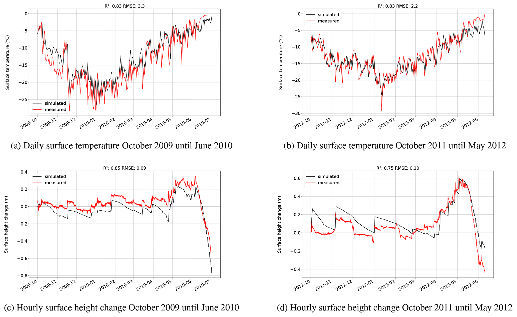
Figure 1 Simulated and measured surface temperatures and surface height changes (in both cases, permanent snow cover) at the location of the automatic weather station at the Zhadang glacier.

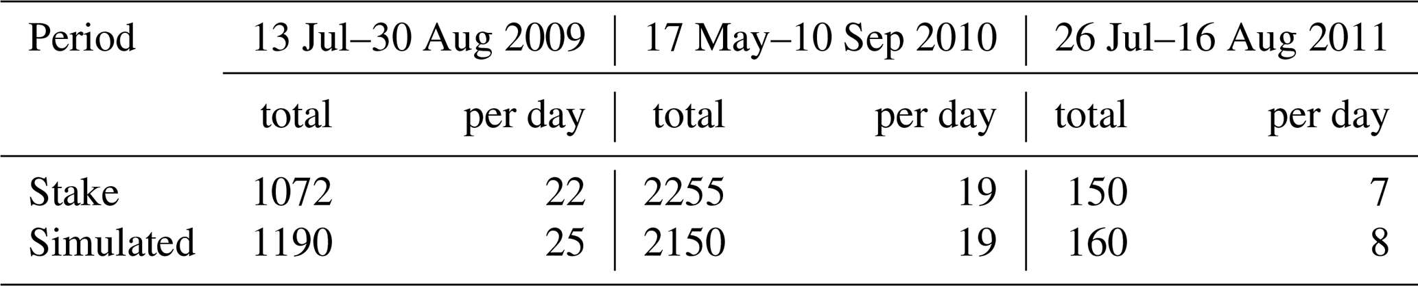
Simulation. Figure 1a and b show the glacier surface temperatures determined from longwave radiation measurements and from COSIPY simulations for two periods where in situ measurements are available. The model represents both the daily variability (R²=0.83, p values <0.001) and the magnitude of the observed surface temperature. The root mean square errors are 3.3 and 2.2 K for the two periods, respectively, and is thus within the typical uncertainty range of longwave radiation measurements. The simulated cumulative mass balance over the entire period from April 2009 to May 2012 is −2.9 m w.e. Figure 1c and d show the simulated and measured ΔH for the two periods (October 2009–June 2010 and October 2011–May 2012) where measurements are available. The daily and seasonal variability is well captured by the model (R²=0.85, p value <0.001 and R²=0.75, p value <0.001), even if snowfall seems to be too low during the first period. Nevertheless, overall, the differences are consistently small with RMSEs of 0.09 and 0.10 m. Table 1 shows the observed and simulated ice ablation for three different periods for which measurements are available. For all three periods, a high degree of agreement is evident, which reveals that the energy fluxes are represented by COSIPY.

Table 1 Observed and simulated ice ablation (mm w.e.) for three periods at the automatic weather station on the Zhadang glacier.

5.1.2 Distributed simulation, scalability

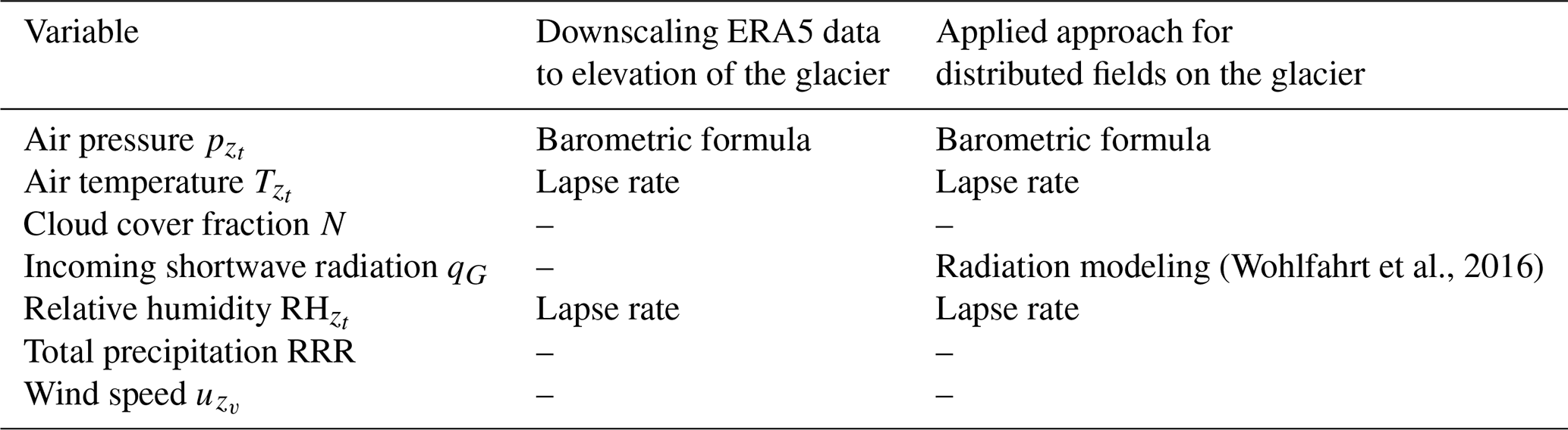
For a distributed glacier-wide run, we drive COSIPY by ERA5 data instead of in situ observations. The ERA5 temperature and humidity data were interpolated across the topography using empirical lapse rates. Atmospheric pressure has been corrected using the barometric formula. The radiation model of Wohlfahrt et al. (2016) was used for the incoming shortwave radiation to account for effects of shadowing, slope and aspect. Total precipitation, cloud cover and horizontal wind velocity were used directly from the closest ERA5 grid point (see Table 2). The computational domain consisted of 1837 grid cells with a spatial resolution of approximately 30 m (1 arcsec) (see Fig. 2).

(Wohlfahrt et al., 2016)

Table 2 COSIPY forcing variables and applied downscaling approaches for distributed simulation. RRR indicates total precipitation.

Simulation. The glacier-wide cumulative surface mass balance for the decade of 2009 to 2018 is presented in Fig. 2. The simulated annual mass balance for this period is −1.9 m w.e. a⁻¹. The results are in line with the analysis of Qu et al. (2014), who reported negative mass balances of −1.9, −2.0, −0.8, and −2.7 m w.e. for the years 2009 to 2012. Furthermore, COSIPY reproduced the spatial distribution at different locations in the ablation area of the Zhadang glacier (see S1, S2, and S3 in Fig. 2b).

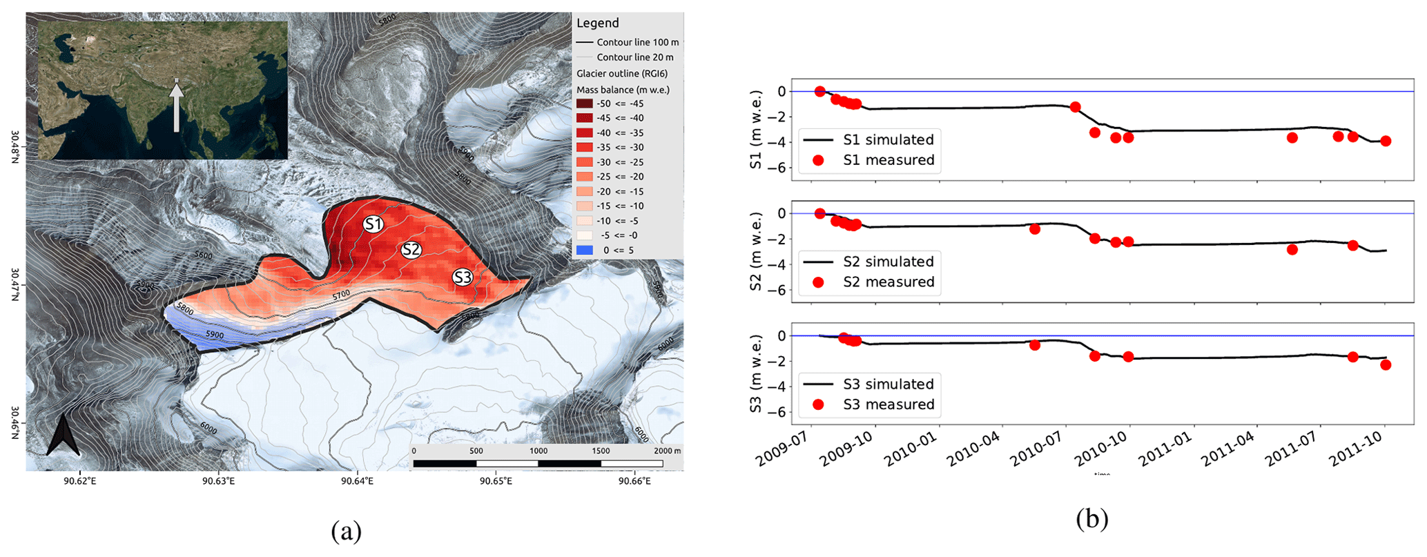
Figure 2 Distributed mass balance simulation of the Zhadang glacier. (a) Cumulative climatic mass balance from 2009 to 2018 with 1827 grid points, contour lines (SRTM), glacier outline from the Randolph Glacier Inventory 6.0, and a topographic map from Bing Maps (Microsoft, 2020); (b) comparison of three measurements (ablation stakes) from July 2009 to October 2011 with the simulated cumulative surface mass balance of the corresponding grid point.

Scalability. A big challenge for large applications is usually the computational cost. To achieve the required performance, models should be scalable on parallel high-performance computing environments. For the model performance analysis, we use a cluster with identical nodes, each consisting of two Intel Xeon(R) E5-2640 v4 CPUs operating at 2.4 GHz and connected via InfiniBand. Each processor has 10 cores, 32 GB memory, and a memory bandwidth of 68.3 GB s⁻¹. To test the performance of the parallelized COSIPY version, we performed a spatial simulation of the Zhadang glacier. We used a 3 arcsec (∼90 m) Shuttle Radar Topography Mission (SRTM) terrain model so that the computational grid consists of 206 points. The performance of the parallel version was then compared to the single-core solution by measuring the required execution time for different core setups (1–220 cores). Figure 3 shows the speedup compared to the single-core version, i.e., the ratio of the original execution time (single core) with the execution time of the corresponding node test (multiple cores). If the model is executed with 20 cores, the speedup is ∼2. With 120 cores, a speedup of ∼10 is reached; i.e., each core has to calculate a maximum of two grid points. A speedup of more than ∼16 is not possible with this system and is achieved with a number of 220 cores (more cores than grid points). The computation time is less than 35 min for a 10-year period (hourly resolution) when using 220 cores. At this point, it should be mentioned that the performance can vary significantly on other HPCC systems and simulation conditions, and should always be checked before submitting larger simulations to the cluster.

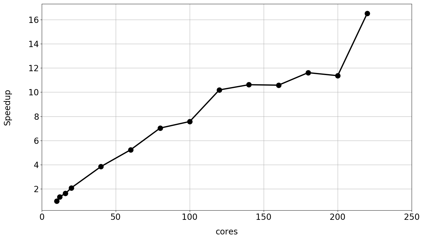
Figure 3 Speedup (execution time of single-core simulation divided by execution time of the corresponding multi-core simulation) for computing a 10-year distributed COSIPY run on the Zhadang glacier with 206 grid points.

5.2 Distributed mass and energy balance simulation and operational application at Hintereisferner in the Austrian Alps

The Hintereisferner (HEF) is a valley glacier located in the Ötztal Alps of Austria (46.79^∘ N, 10.74^∘ E). The glacier begins high on the flank of the Weißkugel mountain, at approximately 3720 m, and runs down to its terminus at approximately 2460 m. HEF is a prime location for meteorological and glaciological research activities due to its monitoring infrastructure. There is a network of four AWSs and four precipitation gauges operated on, and in the vicinity of, HEF. Since 2016, the University of Innsbruck has also been running a permanent terrestrial laser scanner (TLS) and a 5 m meteorological flux tower. Measurement data are transmitted hourly to a data server. COSIPY is now being used to develop an operational mass balance prediction system for the Hintereisferner. The model is driven by the latest Consortium for Small-scale Modeling (COSMO2) analysis and forecast data (see Fig. 4). With the forecast data, the energy and mass flows on the glacier are predicted for the next 24 h with a horizontal resolution of 30 m. The simulated fields are automatically visualized and provided on a web server. In the future, the TLS measurements will be used to improve the forecast continuously. The system is currently running in test mode but will be available to the public in spring 2021.

In addition to the energy and mass flows at the surface, the snow/ice profiles will be stored. This will allow us to compare the results with snow pits and to test the implementation of different parameterizations.

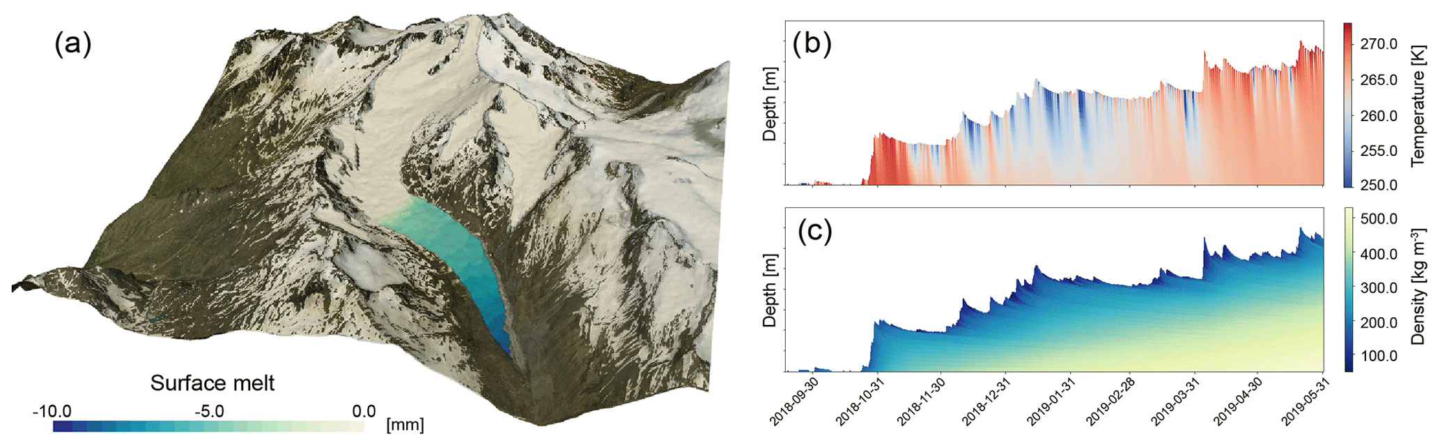
Figure 4 Operational application of COSIPY for the Hintereisferner. Panel (a) shows the forecast of surface melt for 22 June 2020 based on COSMO2 data. Panels (b) and (c) show an example of the temperature and density profile for one site on the glacier tongue for the period of September 2018 to June 2019.

5.3 Model intercomparison – Earth System Model–Snow Model Intercomparison Project

Within the Earth System Model–Snow Model Intercomparison Project (ESM-SnowMIP; Krinner et al., 2018), several of snow models were compared to evaluate different snow schemes and to improve the coupling of land surface snow models in Earth system models. Ménard et al. (2019) describes the standardized input and evaluation data. A total of 10 different sites representing mountainous regions (Europe and the western US), boreal forests (Canada), the Arctic (Finland), and urban regions (Japan) for periods between 7 and 20 years (hourly resolution) are provided, including meteorological classification and details on measuring instruments and data processing. These quality-controlled data are freely available on a PANGAEA repository (Ménard and Essery, 2019) and provide the possibility to benchmark new model developments, detect uncertainties, and reduce model errors. Unlike most of the models participating in the intercomparison project, COSIPY is not a pure snow model, but still all necessary forcing variables are available to apply the model to the different test data sets. We downscaled wind speed from 10 to 2 m above ground using the logarithmic wind profile and calculated the relative humidity from the specific humidity using the saturation mixing ratio and water vapor. The simulated albedo, snow water equivalent (SWE), and snow depth were compared with the evaluation data offered on the online repository (https://doi.org/10.1594/PANGAEA.897575, Ménard and Essery, 2019). Surface and soil temperature could not be compared, because no soil scheme is implemented in COSIPY which allows for warm surface and underground temperatures above the melting point. Figure 5 shows the daily long-term mean values of albedo, SWE, and snow depth for two example sites. The albedo parameterization was calibrated to fit the observed values at Col de Porte. With the calibrated albedo parameterization, COSIPY can reproduce the observed long-term snowpack evolution. The results for Sodankylä, Finland (see Fig. 5b), show a slightly lower snowpack compared to the measurements. The COSIPY runs for both sites are in the range of the ESM-SnowMIP ensemble simulations (see Fig. 5; Krinner et al., 2018).

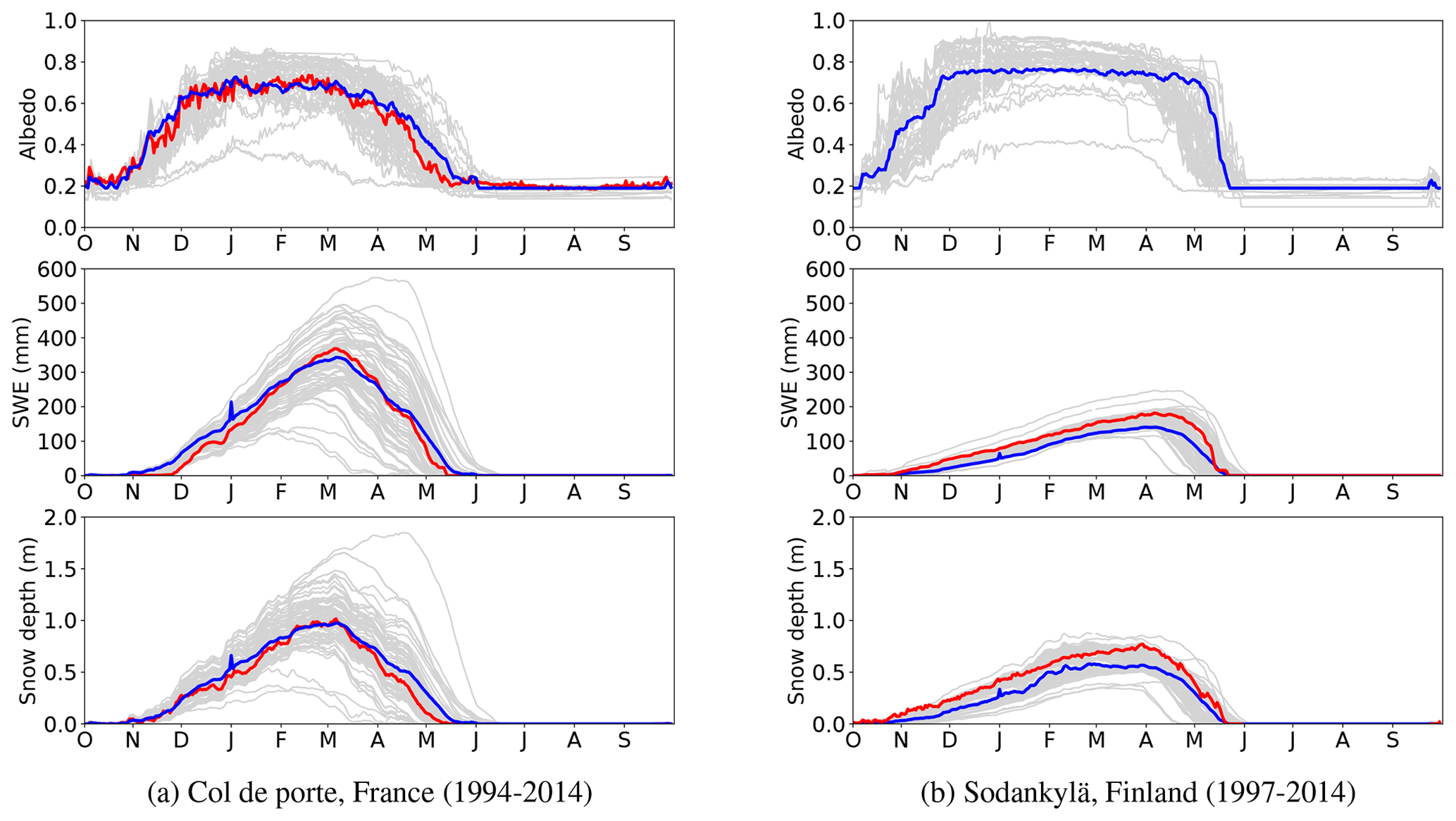
Figure 5 Comparison of long-term daily mean COSIPY with ESM-SnowMIP simulations for two sites. COSIPY simulations (blue lines), measurements (red lines), and ESM-SnowMIP (grey lines) simulations of albedo, snow water equivalent (SWE), and snow depth at two sites. Measurements and simulations provided by Krinner et al. (2018).

6 Conclusions

COSIPY provides a lean, flexible, and user-friendly framework for modeling distributed snow and glacier mass changes. It provides a suitable platform for sensitivity, detection, and attribution analyses as well as a tool for the quantification of inherent uncertainties in mass balance studies. The model has a modular structure and allows the exchange of routines or parameterizations of individual physical processes with little effort. This structure allows the end user to quickly adapt the model to their needs. The open design of COSIPY is well documented, and the modular approach allows joint community-driven further development of the model in the future. In order to increase user friendliness, additional functions are available, such as a restart option for operative applications and an automatic comparison between simulation and ablation data. These functions will be further refined in the future.

The model is written in Python and completely based on open-source libraries. The model, source code, case studies, and code examples for data preprocessing are provided on a freely accessible Git repository (https://github.com/cryotools/cosipy, last access: 11 November 2020) for non-profit purposes. The aim is to set up a community platform where scientists can actively participate in extending and improving the model code. To ensure quality control of the model code, changes to the code are automatically tested with Travis CI (http://www.travis-ci.org, last access: 11 November 2020) when they are uploaded to the repository. It is planned to release updates at regular intervals. To make working with COSIPY easier, a community platform (https://cosipy.slack.com, last access: 11 November 2020) has been set up in addition to the “Read the Docs” documentation (https://cosipy.readthedocs.io/en/latest, last access: 11 November 2020), which allows users and developers to share experiences, report bugs, and communicate needs.

Future improvements of COSIPY are expected by applying the model in different climates and varying topographical settings. Additional processes affecting the climatic mass balance of glaciers such as debris cover and snowdrift can be considered in further developments of the model. In the long run, one of the priorities will be to create a multiphysics environment that allows ensemble runs. In principle, it is already possible to create ensemble simulations with different physical parameterizations and solvers, but COSIPY is not yet an ensemble multiphysics modeling environment. As a vision for the future, it is conceivable to extend COSIPY for automatic ensemble simulations. So far, it is only possible to run COSIPY with different combinations of physical parameterizations or input uncertainties and then evaluate the statistics.

Appendix A

Table A1 List of symbols.