Modeling lightning observations from space-based platforms (CloudScat.jl 1.0)

We describe a computer code that simulates how a satellite observes optical radiation emitted by a lightning flash after it is scattered within an intervening cloud. Our code, CloudScat.jl, is flexible, fully open source and specifically tailored to modern instruments such as the Modular Multispectral Imaging Array (MMIA) component of the Atmosphere–Space Interactions Monitor (ASIM) that operates from the International Space Station. In this article, we describe the algorithms implemented in the code and discuss several applications and examples, with an emphasis on the interpretation of MMIA data.

1 Introduction

Lightning flashes emit intense optical radiation that, after passing through the cloud layer, can be observed from space. This has been applied to characterize the geographic and seasonal distributions of lightning (Christian et al., 2003; Cecil et al., 2014), to describe and forecast the development of particular thunderstorms (Peterson, 2019) and to investigate phenomena related to lightning, such as transient luminous events (TLEs) (Ebert et al., 2010; Pasko et al., 2012) and terrestrial gamma ray flashes (TGFs) (Dwyer et al., 2012; Neubert et al., 2020).

Several satellite-borne instruments targeting lightning optical emissions have been commissioned over the past few years and new ones are planned for the near future. The first such device was the Optical Transient Detector (OTD) (Christian et al., 2003), which was active from 1995 to 2000 onboard the Microlab-1 satellite. The OTD was a model for the longer-lasting Lightning Imaging Sensor (LIS) that operated from the Tropical Rainfall Measurement Mission (TRMM) satellite from 1997 to 2015 (Boccippio et al., 2002; Mach et al., 2007; Zhang et al., 2019; Blakeslee, 2019). A second, identical LIS device has been operating on the International Space Station (ISS) since 2017 (Blakeslee et al., 2016).

After the success of space-based lightning observations from the OTD and LIS, it became desirable, for operational weather prediction, to access real-time lightning data over a large geographic area. This was achieved by the Geostationary Lightning Mapper (GLM) instruments onboard the Geostationary Operational Environmental Satellites (GOES) GOES-East and GOES-West (Goodman et al., 2013) and the Lightning Mapping Imager (LMI) on the FENGYUN (FY-4) satellites. Also, the Meteosat Third Generation (MTG) constellation of satellites will be equipped with lightning-dedicated instruments named Lightning Imagers (LI).

All of these instruments focus only on the detection of lightning flashes and rely on cameras with wavelength filters centered around 777.4 nm, which is a strong emission line of lightning. Their integration times are around 2 ms, and their pixel sizes cover a few kilometers on the ground.

Other instruments target not only lightning but also additional phenomena associated with lightning. The Imager for Sprites and Upper Atmospheric Lightning (ISUAL) payload on the FORMOSAT-2 satellite contained limb-pointing cameras, spectrophotometers and a photometer array designed for the observation of TLEs between the cloud tops and the lower ionosphere (Chern et al., 2003). Although not its main focus, ISUAL detected routinely optical emissions from lightning. The Global Lightning and sprIte MeasurementS (GLIMS) mission, installed on the ISS, was equipped with imagers and photometers to observe lightning and TLEs towards the nadir (Sato et al., 2011; Adachi et al., 2016).

Our work is mainly motivated by another instrument that also has TLEs among its science objectives: the Modular Multispectral Imaging Array (MMIA), which is part of the Atmosphere–Space Interactions Monitor (ASIM) currently onboard the ISS (Chanrion et al., 2019; Neubert et al., 2020). Pointing towards the nadir of the ISS, MMIA is composed of two cameras and three photometers. The cameras provide images filtered at around 777.4 and 337 nm, with the latter wavelength being characteristic of nonthermal discharges that often accompany lightning flashes or are part of them. The camera pixels have a footprint on the ground of around 400 m×400 m at nadir and an integration time of 83.3 ms (yielding 12 frames per second). Of the three photometers, two are sensitive to the same wavelengths as the cameras whereas the third detects an ultraviolet band between approximately 180 and 230 nm. The photometers operate at 10⁵ samples per second. The high spatial resolution of the MMIA cameras and the high temporal resolution of its photometers enable detailed observations of lightning flashes that are, nevertheless, conditioned by scattering within the intervening clouds. This is why this instrument demands an improved understanding of this scattering.

In order to interpret the observations of the instruments mentioned above, one must understand how the optical radiation emitted by a lightning flash is scattered inside a cloud, sometimes with an intricate shape. For example, the strong convection generally associated with active thunderclouds causes overshooting cloud turrets, and the light emerging from them is partially reflected back upwards from the lower cloud deck, as illustrated by Chanrion et al. (2017). Because the optical properties of a lightning flash as observed from above are conditioned by the properties of the cloud where it originated, they may serve to characterize thunderstorms, as recently proposed by Peterson (2019), and also to investigate the time structure of lightning discharges (Peterson and Rudlosky, 2019).

Quantitative models of optical lightning radiation passing through clouds have been developed in the past by researchers such as Thomason and Krider (1982), Koshak et al. (1994) and Light et al. (2001), but these models have been limited to relatively simple cloud geometries and only considered how the radiation is delayed, disregarding image composition.

Here, we present CloudScat.jl, a code that overcomes these two limitations and serves as an open-source tool for the interpretation of space-based lightning observations. CloudScat.jl deals efficiently with complex cloud shapes defined by the composition of elemental solids such as spheres, cylinders and cones that can be arbitrarily placed and deformed. It also predicts the images recorded from observing devices located anywhere relative to the lightning source.

2 Model and numerical algorithm

Our algorithm is partly based on those described by Thomason and Krider (1982) and Light et al. (2001), but it has been extended with additional physical processes and variance-reducing methods. It simulates the propagation of a set of photon packets that interact with a background that includes both cloud hydrometeors and the molecular components of air. As the types of processes that we consider do not change the photon's wavelength, we only consider a monochromatic population of photons with a certain wavelength λ in each simulation. Our model is applicable for wavelengths from around 200 nm to 1 µm.

Every photon packet propagates asynchronously and independently of all other packets; therefore, we describe the dynamics of a single packet in the following. We will also sometimes use the term “photon” as a shortened way of referring to a computational particle, which should, in reality, be considered as an ensemble of physical photons. Each of these photon packets or computational particles is assigned a statistical weight to account for the different number of physical particles that it represents.

We consider two types of processes: scattering processes that modify the propagation direction of the photons are modeled as a series of discrete, stochastic events; and molecular absorption is treated as a continuous process that dampens the statistical weight of the packet as it propagates.

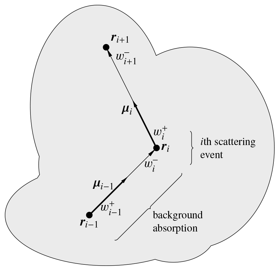
Figure 1 Sketch with the notation employed in this work. We account for two types of processes affecting photon propagation. Mie and Rayleigh scattering are modeled as discrete scattering events that take place at locations ${\mathit{r}}_{\mathrm{1}},\mathrm{\dots },{\mathit{r}}_{i-\mathrm{1}},{\mathit{r}}_i,{\mathit{r}}_{i+\mathrm{1}},\mathrm{\dots }$. Because Mie scattering dissipates part of the photon's energy, in the ith scattering event the particle's statistical weight changes from $w_i^{-}$ to $w_i^{+}$. The absorption by background molecular components of air modifies the particle's statistical weight as it propagates between consecutive scattering events. This changes the particle's weight, e.g., from $w_{i-\mathrm{1}}^{+}$ immediately after scattering i−1 to $w_i^{-}$ immediately before scattering i.

Regarding the discrete scattering events, our notation is that the ith collision takes place at location r_i and time t_i (see Fig. 1). Immediately before the collision the photon weight is $w_i^{-}$ and its velocity is cμ_i−1, where c is the speed of light, and μ_i−1 is a unitary vector. The collision instantaneously changes these magnitudes to $w_i^{+}$, cμ_i. Due to background absorption, the weight decays through the propagation path of a photon so $w_{i+\mathrm{1}}^{-}\le w_i^{+}$, with equality holding in the absence of absorption. All photons are initialized at t₀=0 with weight $w_{\mathrm{0}}^{+}=\mathrm{1}$, with random locations r₀ uniformly distributed in one straight segment and with an isotropic distribution of μ₀. All of our output results are divided by the number of initial photons N, so intensities must be interpreted as intensity per physical photon in the source (equivalently, we could initialize all weights to 1∕N, but this would complicate our description).

As a photon advances, it collides with background scatterers at a total rate per unit time

$$\begin{array}{}\text{(1)}& \mathit{\nu }\left(\mathit{r}\right)=c\sum _{p=\mathrm{1}}^m{\overline{\mathit{\sigma }}}_p\left(\mathit{r}\right)n_p\left(\mathit{r}\right),\end{array}$$

where c is the speed of light, ${\overline{\mathit{\sigma }}}_p\left(\mathit{r}\right)$ is the locally averaged cross section and n_p(r) the number density of the scatterers involved in the process p at location r. The cross sections are averaged locally because a full spectrum of scattering particles with different cross sections may exist around a given point (due to, for example, the different radii of cloud droplets). To sample the interaction times, we employ the null collision method, whereby we find one rate ν_T such that ν_T>ν(r) everywhere inside the computational domain. The time of the ith scattering, including null collisions, is

$$\begin{array}{}\text{(2)}& t_i=t_{i-\mathrm{1}}+{\mathit{\nu }}_T^{-\mathrm{1}}\left|\log \right({\mathit{\xi }}_{i-\mathrm{1}}\left)\right|,\end{array}$$

where ξ_i are independent random variables uniformly distributed in the interval [0,1). The type of interaction is decided with probabilities allotted proportionally to each individual rate and with the probability $\mathrm{1}-\mathit{\nu }\left(\mathit{r}\right)/{\mathit{\nu }}_T$ for a null collision.

2.1 Mie scattering

In Mie scattering a photon packet with a wavelength λ interacts with a cloud droplet, modeled as a dielectric sphere with a radius R≫λ (van de Hulst, 1981). The cross section of this interaction is

$$\begin{array}{}\text{(3)}& {\mathit{\sigma }}_{\mathrm{Mie}}=Q_{\mathrm{ext}}\left(R\right)\mathit{\pi }{R}^{\mathrm{2}},\end{array}$$

where Q_ext is called the “extinction efficiency” and is generally close to 2 (the fact that this is not 1, as the naive application of geometrical optics would suggest, is called the “extinction paradox” and is discussed at length in studies such as Bohren and Huffman, 1983, p. 107). The incident radiation is partially absorbed by the droplet, letting a fraction ω₀ (called the “single-scattering albedo”) of the energy be reemitted. In our code we account for this absorption by updating the weight from $w_i^{-}$ to $w_i^{+}$ as follows. First we compute a temporary weight $w_i^{\prime }$ as

$$\begin{array}{}\text{(4)}& w_i^{\prime }={\mathit{\omega }}_{\mathrm{0}}{w}_i^{-}.\end{array}$$

If $w_i^{\prime }$ is larger than a prescribed w_min<1, we set $w_i^{+}=w_i^{\prime }$; otherwise, we set $w_i^{+}=\mathrm{1}$ with the probability $w_i^{\prime }$, and $w_i^{+}=\mathrm{0}$ with the probability $\mathrm{1}-w_i^{\prime }$ (i.e., in the second case, we discard the photon). Thus, we avoid computations on photons with so little weight that they do not affect the observations, but we ensure that the expected value of $w_i^{+}$ is $w_i^{\prime }$; thus, the simulation stays unbiased (Iwabuchi, 2006). The default value of w_min is 10⁻².

The outgoing electromagnetic wave after Mie scattering is sampled by deflecting the direction of the incident photon. The scattered intensity per unit solid angle at a given direction forming an angle θ with the incident direction is conventionally named the “phase function”, and here, following Thomason and Krider (1982), we approximate it using the Henyey–Greenstein phase function,

$$\begin{array}{}\text{(5)}& p_{\mathrm{HG}}\left(\mathit{\theta }\right)={\displaystyle \frac{\mathrm{1}-g^{\mathrm{2}}}{(\mathrm{1}+g^{\mathrm{2}}-\mathrm{2}g\cos \mathit{\theta }{)}^{\mathrm{3}/\mathrm{2}}}}.\end{array}$$

By convention, any phase function p(θ) is normalized such that

$$\begin{array}{}\text{(6)}& \underset{\mathrm{0}}{\overset{\mathit{\pi }}{\int }}p\left(\mathit{\theta }\right)\sin \left(\mathit{\theta }\right)d\mathit{\theta }=\mathrm{4}\mathit{\pi }.\end{array}$$

The Henyey–Greenstein phase function is parameterized by g, known as the “asymmetry parameter” which is the average of the cosine of the scattering angle,

$$\begin{array}{}\text{(7)}& g={\displaystyle \frac{\mathrm{1}}{\mathrm{4}\mathit{\pi }}}\underset{\mathrm{0}}{\overset{\mathit{\pi }}{\int }}p\left(\mathit{\theta }\right)\cos \left(\mathit{\theta }\right)\sin \left(\mathit{\theta }\right)\mathrm{d}\mathit{\theta }.\end{array}$$

Given an arbitrary phase function obtained, for example, by an accurate solution of the Mie scattering problem, one can compute an asymmetry parameter through Eq. (7) and then approximate the accurate phase function using the Henyey–Greenstein function with the same g. One advantage of this is that it is simple and efficient to sample the Henyey–Greenstein phase function by inverting the cumulative probability distribution of cos θ. The result is that one can draw a random number s uniformly distributed between −1 and 1 and then set

$$\begin{array}{}\text{(8)}& \cos \mathit{\theta }={\displaystyle \frac{\mathrm{1}}{\mathrm{2}g}}\left[\mathrm{1}+g^{\mathrm{2}}-{\left({\displaystyle \frac{\mathrm{1}-g^{\mathrm{2}}}{\mathrm{1}+gs}}\right)}^{\mathrm{2}}\right].\end{array}$$

To compute the three parameters of Mie scattering, Q_ext, ω₀ and g, which depend on the wavelength of interest and the droplet radius, we solve the Mie problem with the open-source MieScatter.jl code (Wilkman, 2013). The refractive index of the medium is a required input for the Mie solver, and the code allows the user to specify this from an input file. The uppermost layers of a thundercloud are above the glaciation line, so the water content is predominantly in ice form. Nevertheless, the optical constants of water and ice are rather similar, with the main difference being that absorption in ice is negligible in the range of wavelengths from 200 to 400 nm (Warren and Brandt, 2008); therefore, for the sake of simplicity, we mostly employ the water optical constants, which we interpolate from Hale and Querry (1973). In most cases reported here, the difference between ice and water is rather small, and we will only consider ice clouds when studying far-ultraviolet radiation in Sect. 3.2.

In general, the droplet size spectrum of a convective cloud is inhomogeneous and assuming a constant radius everywhere may be an oversimplification. A somewhat more accurate model approximates the full spectrum of radii with a single, effective radius R but allows it to depend on the scattering position. In that case, the average cross section as well as the phase function depend on the location of the scattering event. This can optionally be implemented in the code by using a parameterized dependence of the Mie scattering features as a function of R. After inspecting plots of accurate solutions and aiming for simplicity, we settled on these expressions to which we do not attribute any physical meaning:

$$\begin{array}{}\text{(9a)}& {\displaystyle }{Q}_{\mathrm{ext}}\left(R\right)=\mathrm{2}+b{R}^{-\mathrm{3}/\mathrm{4}},\text{(9b)}& {\displaystyle }{\mathit{\omega }}_{\mathrm{0}}\left(R\right)=\mathrm{1}-aR,\text{(9c)}& {\displaystyle }g\left(R\right)={\displaystyle \frac{g_{\mathrm{0}}R}{R+R_{\mathrm{0}}}},\end{array}$$

where a, b, g₀ and R₀ are fitting parameters. These functions are simple but still capture the dependence of the scattering parameters on R. The user of our code can ask to solve the Mie scattering problem for a range of radius $\mathrm{1}\mathrm{\mu }\mathrm{m}<R<\mathrm{100}\mathrm{\mu }\mathrm{m}$, fit the results to the above functions and use the result to build an inhomogeneous model for the cloud.

2.2 Rayleigh scattering

As optical radiation travels inside the cloud or in the path to a space platform, it is also affected by interactions with the molecular components of air. For lightning emissions, this is generally a negligible correction, but we included these interactions in our code for the sake of completeness and to eventually allow for additional applications.

To compute the Rayleigh scattering cross section, we follow Bodhaine et al. (1999), which gives

$$\begin{array}{}\text{(10)}& {\mathit{\sigma }}_{\mathrm{R}}={\displaystyle \frac{\mathrm{24}{\mathit{\pi }}^{\mathrm{3}}F\left(\text{air}\right)}{{\mathit{\lambda }}^{\mathrm{4}}{N}_{\mathrm{0}}^{\mathrm{2}}}}{\left({\displaystyle \frac{n_{\mathrm{s}}^{\mathrm{2}}-\mathrm{1}}{n_{\mathrm{s}}+\mathrm{2}}}\right)}^{\mathrm{2}},\end{array}$$

where N₀ is the number density of air at standard temperature and pressure (the Loschmidt constant), n_s is the refractive index of air under those conditions and F(air) is a so-called “depolarization term” or “King factor”, which corrects the Rayleigh theoretical estimates to account for the asymmetry of scattering molecules. We compute n_s as suggested by Peck and Reeder (1972):

$$\begin{array}{}\text{(11)}& \begin{array}{rl}{\mathrm{10}}^{\mathrm{8}}(n_{\mathrm{s}}-\mathrm{1})& =\mathrm{8060.51}+{\displaystyle \frac{\mathrm{2}\mathrm{480}\mathrm{990}}{\mathrm{132.274}-{\mathit{\lambda }}^{-\mathrm{2}}}}\\ & +{\displaystyle \frac{\mathrm{17}\mathrm{455.7}}{\mathrm{39.32957}-{\mathit{\lambda }}^{-\mathrm{2}}}},\end{array}\end{array}$$

where λ is expressed in micrometers. We calculated F(air) from the formulas provided by Bates (1984), as also compiled by Bodhaine et al. (1999) with the air composition from (Haynes, 2016, p. 14–19).

The phase function for Rayleigh scattering is

$$\begin{array}{}\text{(12)}& p_{\mathrm{R}}\left(\mathit{\theta }\right)={\displaystyle \frac{\mathrm{3}}{\mathrm{4}}}(\mathrm{1}+{\cos }^{\mathrm{2}}\mathit{\theta }),\end{array}$$

and, after inverting the cumulative probability distribution of cos θ, one finds that the phase function can be sampled by setting

$$\begin{array}{}\text{(13)}& \cos \mathit{\theta }=w^{\mathrm{1}/\mathrm{3}}-w^{-\mathrm{1}/\mathrm{3}},w=\mathrm{2}s+(\mathrm{4}{s}^{\mathrm{2}}+\mathrm{1}{)}^{\mathrm{1}/\mathrm{2}},\end{array}$$

where s is a random number uniformly distributed in $[-\mathrm{1},\mathrm{1})$.

The collision rate reads ν_R=cN(z)σ_R, where N(z) is the number density of air at a given altitude z. Because Rayleigh scattering is a small correction on top of the much more relevant Mie scattering, we implemented a simple model where the air density decreases exponentially with altitude:

$$\begin{array}{}\text{(14)}& N\left(z\right)=N_{\mathrm{0}}\exp (-z/H),\end{array}$$

where H is the scale height, which is configurable by the user and defaults to 7.2 km.

2.3 Background absorption

Some wavelengths of interest for the observation of lightning are significantly absorbed in air. For example, the band between 180 and 230 nm that is probed by one of the MMIA photometers is affected by molecular absorption by ozone (Molina and Molina, 1986) and by the Schumann–Runge band of molecular oxygen (Minschwaner et al., 1992). Although, in principle, one could incorporate this into our code by an additional discrete process that randomly discards some of the computational particles, it is more efficient, in terms of a lower variance in the output for the same computational time, to continuously adapt the statistical weight of the particles along their propagation.

For a single absorbing species, in the propagation between two collision points r_i and r_i+1, the weight of the photon changes according to the Beer–Lambert law:

$$\begin{array}{}\text{(15)}& w_{i+\mathrm{1}}^{-}=w_i^{+}\exp \left(-\underset{{\mathit{r}}_i}{\overset{{\mathit{r}}_{i+\mathrm{1}}}{\int }}{\mathit{\sigma }}_{\mathrm{abs}}{n}_{\mathrm{abs}}\left(\mathit{r}\right)\mathrm{d}r\right),\end{array}$$

where the integral is along the straight line between r_i and r_i+1, σ_abs is the absorption cross section and n_abs is the number density of the absorbing species.

In our code we implemented the most common case of a stratified atmosphere where n_abs depends only on the altitude z. In that case, we can avoid computing the integral in Eq. (15) for every propagation step. This is implemented by computing a cumulative density during the code initialization:

$$\begin{array}{}\text{(16)}& M\left(z\right)=\underset{\mathrm{0}}{\overset{z}{\int }}{n}_{\mathrm{abs}}\left(z^{\prime }\right)\mathrm{d}{z}^{\prime }.\end{array}$$

This integral is computed within a grid of altitudes and then linearly interpolated for arbitrary z between the grid points. The integral in Eq. (15) can be rewritten as

$$\begin{array}{}\text{(17)}& \underset{{\mathit{r}}_i}{\overset{{\mathit{r}}_{i+\mathrm{1}}}{\int }}{\mathit{\sigma }}_{\mathrm{abs}}{n}_{\mathrm{abs}}\left(\mathit{r}\right)\mathrm{d}r={\displaystyle \frac{{\mathit{\sigma }}_{\mathrm{abs}}\left|M\right(z_{i+\mathrm{1}})-M(z_i\left)\right|}{\left|{\mathit{\mu }}_i^z\right|}},\end{array}$$

where ${\mathit{\mu }}_i^z$ is the z component of the unitary vector pointing from r_i to r_i+1 and we assumed ${\mathit{\mu }}_i^z\ne \mathrm{0}$. In the unlikely case that, within working precision, the photon propagation is horizontal, we have

$$\begin{array}{}\text{(18)}& \underset{{\mathit{r}}_i}{\overset{{\mathit{r}}_{i+\mathrm{1}}}{\int }}{\mathit{\sigma }}_{\mathrm{abs}}{n}_{\mathrm{abs}}\left(\mathit{r}\right)\mathrm{d}r={\mathit{\sigma }}_{\mathrm{abs}}n\left(z_i\right)|{\mathit{r}}_{i+\mathrm{1}}-{\mathit{r}}_i|.\end{array}$$

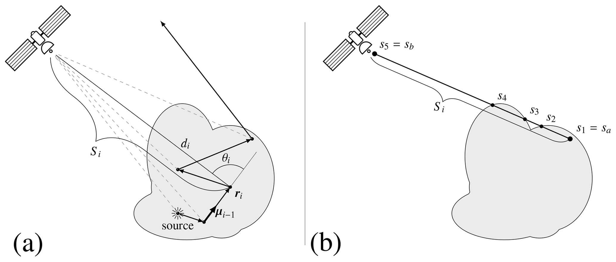
Figure 2 Outline of the local estimation method. (a) For a given packet we add the contributions to the radiated energy reaching a detector from each scattering event. (b) These contributions are affected by the optical depth of the scattering location, which involves an integral from that point to the detector. The integral is divided into segments where the collision rate is smooth.

2.4 Local estimation method

Typically, in our code we consider 10⁶ to 10⁷ photon packets, and we simulate the signal received by an observer hundreds of kilometers away from the source. With these numbers, the probability that a significant number of photons packets would emerge from the area covered by one image pixel and reach the detector is negligible. For this reason, we cannot simulate an image by accounting only for the final, outgoing direction of the simulated photons. We overcome this problem by means of a local estimation method as described in studies such as Iwabuchi (2006). This method is sketched in Fig. 2a and may be understood as follows.

After the ith collision, the energy of the photon packet is radiated in all directions according to the incident direction μ_i−1 and the phase function p(θ) (either p_R or p_HG). Consider a detector with a surface area A at a large distance d_i from the scattering event with $A\ll \mathrm{4}\mathit{\pi }{d}_i^{\mathrm{2}}$. The energy that reaches this detector is

$$\begin{array}{}\text{(19)}& {\mathit{\delta }}_i={\displaystyle \frac{A{w}_i^{-}p\left({\mathit{\theta }}_i\right)}{\mathrm{4}\mathit{\pi }{d}_i^{\mathrm{2}}}}\exp (-{\mathit{\tau }}_i),\end{array}$$

where the energy is normalized to that of a photon of the given wavelength with unitary weight, θ_i is the angle between μ_i−1 and the line of sight S_i of the event r_i, and τ_i is the optical depth defined as

$$\begin{array}{}\text{(20)}& {\mathit{\tau }}_i=\underset{S_i}{\int }{\mathit{\nu }}_{\mathrm{all}}\left(s\right)\mathrm{d}s,\end{array}$$

where s is a coordinate indexing the line of sight S_i (with length d_i), and ν_all includes all processes that may affect a photon (Mie scattering, Rayleigh scattering and background absorption). During a simulation we bin all δ_i according to their direction of arrival to the detector to form an image or according to their arrival time $t_i^{\prime }=t_i+d_i/c$ to simulate a photometer waveform. For this purpose, to set up a run the user must specify the features of one or several observing devices, including their location and the field of view and image size of their cameras as well as the frame rate of their photometers. In all photometer plots in this paper our initial time is the time of arrival of a hypothetical unscattered source photon.

The components of τ_i stemming from Rayleigh scattering and background absorption are computed using an analytical expression for Rayleigh scattering and with the method described in the previous section for background absorption, which is trivially adapted for the propagation towards an observer.

However, for a general cloud geometry, the integration path in Eq. (20) sometimes traverses several cloud boundaries (see Fig. 2b) where the Mie component of the collision rate (ν_Mie) presents discontinuities. We take this into account by dividing the path $S_i=(s_a,s_b)$ into n subintervals $(s_{\mathrm{1}}=s_a,s_{\mathrm{2}})$, …, $(s_n,s_{n+\mathrm{1}}=s_b)$ and rewriting the integral as

$$\begin{array}{}\text{(21)}& {\mathit{\tau }}_{i,\text{Mie}}=\sum _{k=\mathrm{1}}^n\underset{s_k}{\overset{s_{k+\mathrm{1}}}{\int }}{\mathit{\nu }}_{\mathrm{Mie}}\left(s\right)\mathrm{d}s,\end{array}$$

where we can assume each integrand to be smooth. Each integral, from s_k to s_k+1 is computed numerically via a Gauss–Legendre quadrature with an order that defaults to 3 but can be configured by the user.

The integrals in Eq. (21) are computationally expensive and take a significant portion of the computations. In some cases, however, they can be skipped: if a scattering event happens deep within the cloud, τ_i is so large that the contribution of δ_i is negligible. To account for this and save computational time, the user can select a minimum altitude z_min below which Eq. (21) is not computed and the corresponding δ_i is set to zero.

Note that in the local estimation method a single photon packet leaves observation traces from more than a single time and place and, thus, creates spurious correlations in the predicted observations. These correlations are visible when the simulated signal is weak, but they do not pose a practical concern.

2.5 Cloud geometry

The CloudScat code admits arbitrarily complex cloud geometries. The user constructs the cloud shape by means of Boolean combinations and affine transformations of elementary solid figures. The code is equipped with a library of figures including a sphere, a cylinder, a cone and a half-space delimited by a plane. This can be extended with user-defined figures by implementing methods that (a) compute the intersections of the figure's boundary with a straight line and (b) determine whether the figure contains a given point.

The supported Boolean operations are:

1. union of several figures F₁…F_M – a point is contained in the union ${\cup }_{i=\mathrm{1}}^M{F}_i$ if it is contained in any F_i;

2. intersection of several figures F₁…F_M – a point is contained in the intersection ${\cap }_{i=\mathrm{1}}^M{F}_i$ if it is contained in all F_i;

3. difference of two figures F₁ and F₂ – a point is contained in the difference F₁∖F₂ if it is contained in F₁ but not in F₂.

These operations can be nested to an arbitrary depth, constructing, for example, the difference between a union and an intersection.

The figures (and any Boolean combination thereof) can also be modified by affine transformations 𝒜 consisting of a translation vector R and an invertible matrix M. A point r belongs to the transformed figure 𝒜F if ${\mathit{r}}^{\prime }={\mathbf{M}}^{-\mathrm{1}}\mathit{r}-\mathit{R}$ belongs to F. This means linearly transforming the shape with M and afterwards translating it along R. Again, affine transformations can be combined with other affine transformations and Boolean operations up to an arbitrary depth.

3 Examples and applications

3.1 Photon diffusion model

In part as a verification of the code and in part as a modeling tool, we first consider the heavily simplified case of a point-like lightning source inside a homogeneous, infinite cloud with a planar top that we set at z=0. In this section, we also neglect Rayleigh scattering and background absorption and set a homogeneous collision rate ν=cN_dQ_extπR², where N_d is a droplet number density, and Q_ext and R are the respective extinction coefficient and droplet radius, which are also assumed to be homogeneous.

Koshak et al. (1994) applied classical methods of transport theory to the problem of radiation propagation inside a cloud. By truncating the spherical-harmonic expansion of the one-speed Boltzmann equation, they showed that the photon density ψ approximately follows a diffusion equation with an absorption term:

$$\begin{array}{}\text{(22)}& {\displaystyle \frac{\partial \mathit{\psi }}{\partial t}}-\mathrm{\nabla }\cdot \left(D\mathrm{\nabla }\mathit{\psi }\right)=-{\displaystyle \frac{\mathit{\psi }}{{\mathit{\tau }}_{\mathrm{A}}}},\end{array}$$

where the diffusion coefficient D is

$$\begin{array}{}\text{(23)}& D={\displaystyle \frac{c^{\mathrm{2}}}{\mathrm{3}\mathit{\nu }(\mathrm{1}-g{\mathit{\omega }}_{\mathrm{0}})}},\end{array}$$

and

$$\begin{array}{}\text{(24)}& {\mathit{\tau }}_{\mathrm{A}}={\displaystyle \frac{\mathrm{1}}{\mathit{\nu }(\mathrm{1}-{\mathit{\omega }}_{\mathrm{0}})}}\end{array}$$

is the photon absorption time. Equation (22) must be supplemented by the condition $\mathit{\psi }(z=\mathrm{0})=\mathrm{0}$ imposed by the perfectly absorbing boundary (photons at locations z>0 never reach the cloud again).

The solution of Eq. (22) with the appropriate boundary condition and initial condition $\mathit{\psi }(\mathit{r},t=\mathrm{0})=\mathit{\delta }\left(x\right)\mathit{\delta }\left(y\right)\mathit{\delta }(z-L)$, corresponding to a point source at $(\mathrm{0},\mathrm{0},-L)$, is found by the method of images (Krapivsky et al., 2010, p. 32) and reads

$$\begin{array}{}\text{(25)}& \begin{array}{rl}\mathit{\psi }(x,y,z)& ={\displaystyle \frac{e^{-t/{\mathit{\tau }}_{\mathrm{A}}}}{(\mathrm{4}\mathit{\pi }Dt{)}^{\mathrm{3}/\mathrm{2}}}}\left[\exp \left({\displaystyle \frac{-x^{\mathrm{2}}-y^{\mathrm{2}}-(z+L{)}^{\mathrm{2}}}{\mathrm{4}Dt}}\right)\right.\\ & \left.-\exp \left({\displaystyle \frac{-x^{\mathrm{2}}-y^{\mathrm{2}}-(z-L{)}^{\mathrm{2}}}{\mathrm{4}Dt}}\right)\right].\end{array}\end{array}$$

From this expression, one obtains the instantaneous flux of photons emerging from the cloud at coordinates ($x,y,\mathrm{0}$) and time t as

$$\begin{array}{}\text{(26)}& \begin{array}{rl}f(x,y,t)& =D{\left({\displaystyle \frac{\partial \mathit{\psi }}{\partial z}}\right)}_{z=\mathrm{0}}\\ & ={\displaystyle \frac{L{e}^{-t/{\mathit{\tau }}_{\mathrm{A}}}}{(\mathrm{4}\mathit{\pi }D{)}^{\mathrm{3}/\mathrm{2}}{t}^{\mathrm{5}/\mathrm{2}}}}\exp \left({\displaystyle \frac{-x^{\mathrm{2}}-y^{\mathrm{2}}-L^{\mathrm{2}}}{\mathrm{4}Dt}}\right).\end{array}\end{array}$$

Moreover, integrating in the x–y plane, this yields a total flux per unit time

$$\begin{array}{}\text{(27)}& \begin{array}{rl}F\left(t\right)& =\underset{-\mathrm{\infty }}{\overset{\mathrm{\infty }}{\int }}\mathrm{d}x\underset{-\mathrm{\infty }}{\overset{\mathrm{\infty }}{\int }}\mathrm{d}yf(x,y,t)\\ & ={\displaystyle \frac{e^{-t/{\mathit{\tau }}_{\mathrm{A}}-{\mathit{\tau }}_{\mathrm{D}}/t}}{{\mathit{\pi }}^{\mathrm{1}/\mathrm{2}}{\mathit{\tau }}_{\mathrm{D}}}}{\left({\displaystyle \frac{t}{{\mathit{\tau }}_{\mathrm{D}}}}\right)}^{-\mathrm{3}/\mathrm{2}},\end{array}\end{array}$$

where we have introduced the characteristic time for the photons to diffuse up to a distance L,

$$\begin{array}{}\text{(28)}& {\mathit{\tau }}_{\mathrm{D}}={\displaystyle \frac{L^{\mathrm{2}}}{\mathrm{4}D}}.\end{array}$$

On the other hand, integrating Eq. (26) in time gives an expression for the number of photons that exit the cloud from a given location at anytime,

$$\begin{array}{}\text{(29)}& \begin{array}{rl}\mathrm{\Phi }(x,y)& =\underset{\mathrm{0}}{\overset{\mathrm{\infty }}{\int }}\mathrm{d}tf(x,y,t)={\displaystyle \frac{\mathrm{1}}{\mathrm{2}\mathit{\pi }(L^{\mathrm{2}}+{\mathit{\rho }}^{\mathrm{2}})}}\\ & \cdot \left({\displaystyle \frac{L}{(L^{\mathrm{2}}+{\mathit{\rho }}^{\mathrm{2}}{)}^{\mathrm{1}/\mathrm{2}}}}+\mathrm{2}\mathit{ϵ}\right)\exp \left(-{\displaystyle \frac{\mathrm{2}\mathit{ϵ}(L^{\mathrm{2}}+{\mathit{\rho }}^{\mathrm{2}})}{L}}\right),\end{array}\end{array}$$

where we have introduced $\mathit{\rho }=(x^{\mathrm{2}}+y^{\mathrm{2}}{)}^{\mathrm{1}/\mathrm{2}}$ and $\mathit{ϵ}=({\mathit{\tau }}_{\mathrm{D}}/{\mathit{\tau }}_{\mathrm{A}}{)}^{\mathrm{1}/\mathrm{2}}$. In cases where the absorption of photons can be neglected (i.e., the time of absorption τ_A is much larger than the characteristic diffusion time τ_D) Eq. (29) reduces to

$$\begin{array}{}\text{(30)}& \mathrm{\Phi }\left(\mathit{\rho }\right)={\displaystyle \frac{L}{\mathrm{2}\mathit{\pi }(L^{\mathrm{2}}+{\mathit{\rho }}^{\mathrm{2}}{)}^{\mathrm{3}/\mathrm{2}}}},\end{array}$$

which, remarkably, leads to a spatial distribution of optical radiation that does not depend on the Mie scattering parameters but only on the source depth L.

Soler et al. (2020) fitted expression (27) to the MMIA photometer signal in order to infer the altitudes of presumed fast breakdown events (Rison et al., 2016) associated with radio-detected narrow bipolar events (Le Vine, 1980; Smith et al., 1999; Liu et al., 2018). They obtained a best-fit τ_D, and using Eq. (28), given a plausible bracket for D, they derived an interval for L which, combined with independent measurements of the cloud-top height provides a range of source altitudes.

Another approach to estimate the source depth is by means of the spatial distribution described by Eq. (30), which offers the advantage that it does not demand assumptions about D. This is, however, limited to cases where absorption is weak and the irregularities of the cloud top do not affect the recorded image too much. Both of these conditions generally imply that the source is not too deeply buried in the cloud.

Clearly, both of these approaches to estimate the source depth also depend on approximating the source as point-like. This is acceptable for fast breakdown events which span some hundreds of meters (Rison et al., 2016; Tilles et al., 2019) but becomes more questionable for other types of events.

Let us apply our Monte Carlo model to this configuration. We run the code for a point source within an infinite, homogeneous cloud. The cloud top is set at 15 km and the source at 10 km. The cloud is composed of droplets with radius R=10 µm and a density $N_{\mathrm{d}}=\mathrm{100}{\mathrm{cm}}^{-\mathrm{3}}$, and we consider the propagation of radiation with a wavelength λ=337 nm. The resulting Mie scattering parameters are g=0.874, ${\mathit{\omega }}_{\mathrm{0}}=\mathrm{1}-\mathrm{2.82}\times {\mathrm{10}}^{-\mathrm{6}}$ and $Q_{\mathrm{ext}}=\mathrm{2}+\mathrm{3.99}\times {\mathrm{10}}^{-\mathrm{2}}$.

The photons emerging from the cloud have a slight preference for the direction perpendicular to the cloud boundary, so the radiance is not perfectly Lambertian. For the purpose of comparison with the analytical expressions derived above, we must integrate the emissions in all directions. Making use of the azimuthal symmetry of the emissions, we achieve this by setting several observers, all of them at a distance of 400 km from the point in the cloud top closest to the source, but we vary the zenith angle of observation. We chose these angles to perform a five-point Gauss–Legendre quadrature of the photon flux in all directions. Figure 3 compares the Monte Carlo results and expression (27). We consider the agreement of the two curves as a verification of the code implementation as well as of the diffusion model proposed by Koshak et al. (1994).

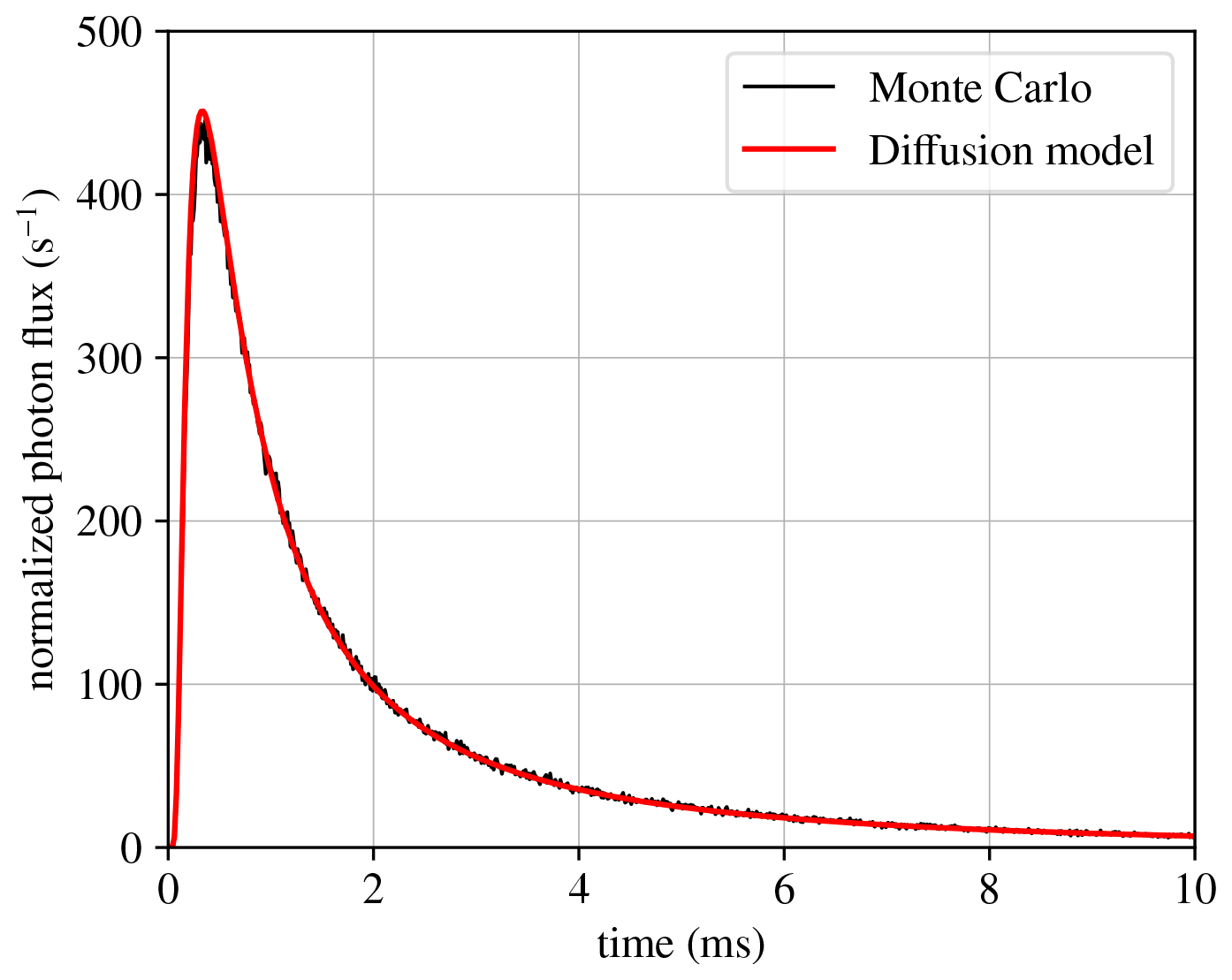
Figure 3 Total photon flux emerging from a semi-infinite cloud. The cloud extends infinitely below 15 km, and the photon source is located at 10 km. We compare a Monte Carlo (black) and an analytically solvable diffusion model (red). The photon flux is normalized with respect to the number of source photons (i.e., it must be interpreted as the flux per source photon). The parameters of the model curve are τ_D=0.503 ms and τ_A=18.5 ms. Here and in all subsequent photometer plots, the time origin corresponds to the arrival time of an unscattered photon.

Our next step is to account for the fact that the cloud is not infinitely deep and, therefore, some photons exit through the lower boundary. We now consider a cloud limited by two infinite parallel planes. The method of images is also suitable for this problem, but the solution is composed of an infinite sum of contributions from virtual images arranged in a periodic lattice. Assume that the cloud extends from z=0 to $z=-b$ and the photon source is again at $z=-L$. The resulting lattice consists of positive images at $z\in \mathit{\{}-L+\mathrm{2}bn:n\in \mathbb{Z}\mathit{\}}$ and negative images at $z\in \mathit{\{}L+\mathrm{2}bn:n\in \mathbb{Z}\mathit{\}}$. The contribution of each image to the integrated flux of photons at z=0 reads

$$\begin{array}{}\text{(31)}& F_n^{\pm }\left(t\right)=\pm {\displaystyle \frac{\mathrm{2}\mathit{\pi }D{e}^{-t/{\mathit{\tau }}_{\mathrm{A}}}}{(\mathrm{4}\mathit{\pi }Dt{)}^{\mathrm{3}/\mathrm{2}}}}(\mp L+\mathrm{2}bn)\exp \left(-{\displaystyle \frac{(\mp L+\mathrm{2}bn{)}^{\mathrm{2}}}{\mathrm{4}Dt}}\right).\end{array}$$

Noting that $F_n^{\pm }=F_{-n}^{\mp }$, we write the total flux as

$$\begin{array}{}\text{(32)}& F\left(t\right)={\displaystyle \frac{\mathrm{4}\mathit{\pi }D{e}^{-t/{\mathit{\tau }}_{\mathrm{A}}}}{(\mathrm{4}\mathit{\pi }Dt{)}^{\mathrm{3}/\mathrm{2}}}}\sum _{n\in \mathbb{Z}}(L+\mathrm{2}bn)\exp \left(-{\displaystyle \frac{(L+\mathrm{2}bn{)}^{\mathrm{2}}}{\mathrm{4}Dt}}\right).\end{array}$$

Notice that if we keep only the n=0 term in this series, we recover expression (27). For long time spans, Eq. (32) requires the unwieldy addition of a large number of terms. Therefore, in order to obtain the long-term behavior of F(t), we use the following identity that results from the Poisson summation formula and is valid for arbitrary u, v:

$$\begin{array}{}\text{(33)}& \begin{array}{rl}& \sum _{n\in \mathbb{Z}}(u+nv)e^{-(u+nv{)}^{\mathrm{2}}}\\ & ={\displaystyle \frac{\mathrm{2}{\mathit{\pi }}^{\mathrm{3}/\mathrm{2}}}{v^{\mathrm{2}}}}\sum _{k=\mathrm{1}}^{\mathrm{\infty }}k\sin \left({\displaystyle \frac{\mathrm{2}\mathit{\pi }ku}{v}}\right)\exp \left(-{\displaystyle \frac{{\mathit{\pi }}^{\mathrm{2}}{k}^{\mathrm{2}}}{v^{\mathrm{2}}}}\right).\end{array}\end{array}$$

This allows us to cast Eq. (32) into

$$\begin{array}{}\text{(34)}& F\left(t\right)={\displaystyle \frac{\mathrm{2}\mathit{\pi }D{e}^{-t/{\mathit{\tau }}_{\mathrm{A}}}}{b^{\mathrm{2}}}}\sum _{k=\mathrm{1}}^{\mathrm{\infty }}k\sin \left({\displaystyle \frac{\mathit{\pi }kL}{b}}\right)\exp \left(-{\displaystyle \frac{{\mathit{\pi }}^{\mathrm{2}}{k}^{\mathrm{2}}Dt}{b^{\mathrm{2}}}}\right),\end{array}$$

which converges faster than Eq. (32) for long t. Indeed, from the slowest decaying term k=1 we extract a decay time

$$\begin{array}{}\text{(35)}& {\mathit{\tau }}_{\mathrm{S}}={\displaystyle \frac{b^{\mathrm{2}}}{{\mathit{\pi }}^{\mathrm{2}}D}}.\end{array}$$

To check our code against these expressions, we run a simulation with the same microscopical parameters as used above for Fig. 3; however, in this case, the cloud exists only above an altitude of 7 km. The photon source is again at 10 km and, thus, closer to the lower boundary than to the cloud top. In this situation we expect Eq. (27) to perform poorly for long time spans. This is indeed the case as we show in Fig. 4, where we plot the Monte Carlo results along with expression (27), which disregards the lower boundary. Also represented are two truncations of the series (34) that keep one and two terms. We see that the long-term behavior is perfectly captured by the k=1 term in the series. At early times, the approximation is much improved by including a second term of the sum. For small t, Eq. (27) is closer to the simulation curve; this is because that expression is a one-term truncation of the series (32), which converges faster as t→0.

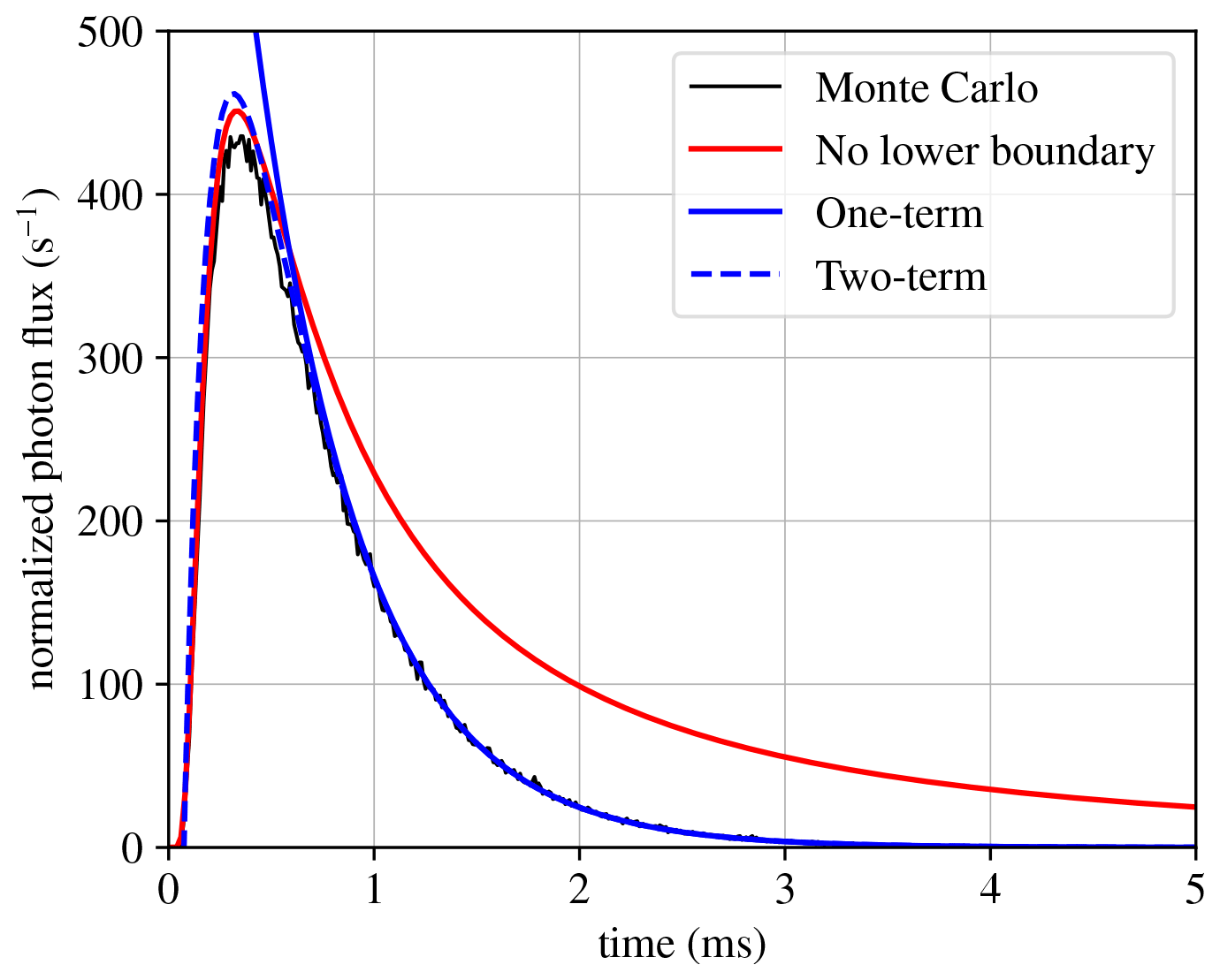
Figure 4 Total photon flux emerging from the top of a planar homogeneous 8 km thick cloud. We plot the Monte Carlo simulation results (black) along with the analytical expression for a cloud without the lower bound (red; same as Fig. 3) and the one- and two-term truncations of the analytical approximation (blue; see text). Note that the two-term approximation reaches unphysical negative values for times shortly after the source pulse, although this is barely discernible in the plot.

3.2 Ozone absorption

As we mentioned above, the absorption of radiation by the molecular components of air cannot be neglected for certain wavelengths. A case in point is the absorption of the far-ultraviolet radiation by ozone in the range from 180 to 230 nm, to which one of the MMIA photometers is sensitive. This photometer was conceived for light emanating from TLEs in the upper atmosphere (Neubert et al., 2020), but it may also be sensitive to lightning emissions. Here, we investigate this possibility by simulating the photometer response to a far-ultraviolet source inside a thundercloud.

We selected a wavelength of 200 nm, where the absorption cross section of ozone reaches a minimum ${\mathit{\sigma }}_{\mathrm{abs}}=\mathrm{3.145}\times {\mathrm{10}}^{-\mathrm{19}}{\mathrm{cm}}^{\mathrm{2}}$ (Molina and Molina, 1986). Therefore, this is the most well-transmitted wavelength, although we do not know if strong emission lines are present around this wavelength in a lightning flash.

The ozone density inside a thunderstorm is also uncertain and may differ significantly from a fair-weather density because it is affected by the strong convection and electrical activity of the thunderstorm (Pan et al., 2014; Bozem et al., 2014). Nevertheless, for illustration purposes, we selected several profiles of ozone in the atmosphere corresponding to those implemented in the MODTRAN 5 code (Berk et al., 2005) as previously introduced by Kneizys et al. (1980) for the LOWTRAN code. They correspond to tropical (15^∘ N), midlatitude summer (45^∘ N, July) and midlatitude winter (45^∘ N, January) conditions as well as to the U.S. Standard Atmosphere (United States Committee on Extension to the Standard Atmosphere, 1976). We disregard subarctic conditions as they are not relevant for lightning. The ozone profiles are displayed in Fig. 5a.

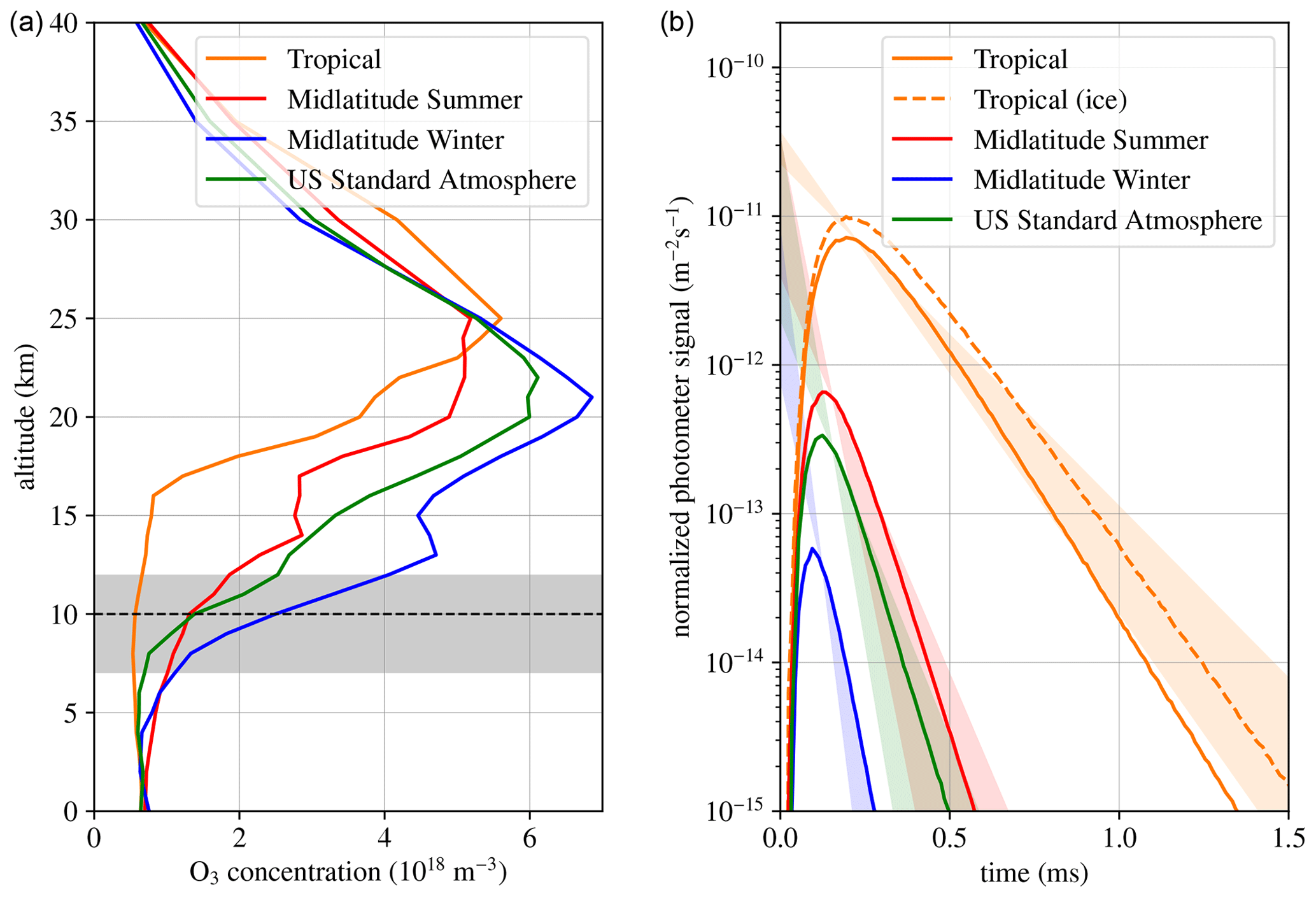
Figure 5 The role of ozone absorption in the photometer signal from a lightning flash. Panel (a) shows several ozone profiles employed in Monte Carlo simulations. The shaded area marks the extent of the cloud, and the horizontal dashed line marks the location of the source. In panel (b), we show the simulated photometer response to a 200 nm source observed from above at an altitude of 400 km. Except in the indicated case, all simulations use the water refractive index. The shaded areas indicate the range of exponential decay rates corresponding to the ozone density at the location of the source and at the cloud top (bear in mind that only the slopes of these curves are relevant: they are placed to pass through the peak of the Monte Carlo curves).

We implemented these ozone profiles in simulations with the same cloud configuration as in the previous section (10 µm droplets with a density of 100 cm⁻³ in a cloud spanning from 7 to 12 km; source at 10 km) but with a 200 nm source. Besides the role of molecular absorption, this wavelength also underlines differences between the absorption properties of water and ice: whereas water absorbs 200 nm radiation strongly, absorption by ice is negligible. However, we observe this difference only when molecular absorption by ozone does not dominate. The tropical case, for example, has the lowest ozone density and, thus, allows us to see different absorption rates between water and ice. Therefore, we run simulations for that ozone profile using both ice and water optical constants. Note also that we are now not interested in the total photon flux emerging from the cloud top; therefore, we simulated the response of a single photometer located at an altitude of 400 km directly above the source.

The results, plotted in Fig. 5b show the signal decaying quickly within a fraction of a millisecond. If the ozone density ($n_{{\mathrm{O}}_{\mathrm{3}}}$) was homogeneous within the cloud, the decay time would be

$$\begin{array}{}\text{(36)}& {\mathit{\tau }}_{{\mathrm{O}}_{\mathrm{3}}}=c{\mathit{\sigma }}_{\mathrm{abs}}{n}_{{\mathrm{O}}_{\mathrm{3}}}.\end{array}$$

However, with the selected profiles, the photons explore regions with markedly different ozone densities. In Fig. 5b, we indicate, by means of a shaded region, the range of decay rates between the source location (slowest decay) and the cloud top (the fastest decay). In most cases, the decay rate is between the two extreme values predicted by the ozone concentrations at the source and at the cloud top. The exception is the tropical ozone profile, where the strong absorption by water droplets leads to a somewhat faster decay. If we use the same ozone profile but employ the ice refractive index, the decay is slower and is within the range predicted by ozone absorption.

It is important to note that although the decay in the observed optical radiation is dominated by ozone absorption in most cases in the geometry considered here, this is not always the case – as we have seen for the tropical ozone profile. Once more, the key is the interplay between the timescales defined in the previous section and the timescales for ozone absorption in the relevant range of altitudes. For example, with a thinner cloud only extending up to 12 km altitude, we clearly see the effect of τ_S as defined above.

3.3 The timescales involved in photometer waveforms

In the previous sections, we introduced four different timescales, summarized in Table 1, which affect the photometer response to a lightning flash. Although these timescales have a closed-form expression only within the simplified models that we have considered so far, they nevertheless provide (also in more realistic settings) a useful framework of analysis. However, it must be noted that a lightning stroke or flash possesses intrinsic timescales left aside in our discussion: the final photometer response results from the convolution of these intrinsic timescales with those introduced by in-cloud scattering.

Our experience leads us to the following broad guidelines for the analysis of photometer pulses:

1. Absorption by ozone molecules (timescale ${\mathit{\tau }}_{{\mathrm{O}}_{\mathrm{3}}}$) is mostly negligible for optical wavelengths but is strong below about 300 nm. Therefore, one expects very short pulses in the ultraviolet, as shown in Fig. 5.

2. Under most circumstances, absorption by droplet or ice particles (measured by τ_A) is relatively weak and is visible only in the tail of the photometer response

3. Usually both the time for diffusion to the cloud top (τ_D) and the total residence time (τ_S) are relevant, with τ_D mostly affecting the rise-time of the signal and τ_S affecting its decay. This is visible in Fig. 4, where the rise is captured by an expression that involves only τ_D, whereas the decay follows an exponential with characteristic time τ_S.

Table 1 Timescales defining the photometer response to an impulsive optical source inside a thundercloud.

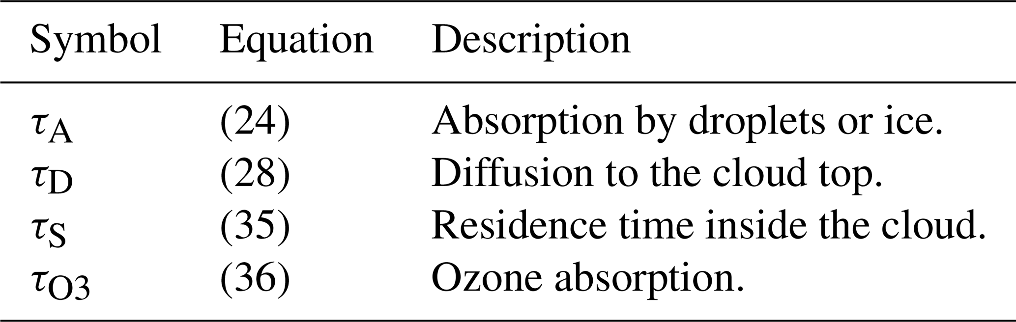
Figure 6 A satellite observes a flash-illuminated complex cloud. The observation geometry is shown in (a), where we represent the cloud geometry and the satellite location. In (b) we show a rendering of the cloud geometry as observed from the satellite's viewpoint. Finally (c) and (d) are the outcome of our Monte Carlo model simulating an image captured by the satellite's camera filtered at 337 and 777 nm, respectively. In this image we have labeled the hole in the cloud turret (1), the emissions from the lower cloud deck (2) and the surrounding, diffuse Rayleigh emissions (3).

3.4 Imaging complex geometries

Let us now turn to the imaging capabilities of the CloudScat.jl code combined with complex cloud shapes. As an example, we construct the following cloud geometry, which roughly mimics a typical convective thundercloud and is shown in Fig. 6a and b. It starts from a cylindrical base with a radius of 20 km and spans altitudes between 7 and 10 km above the ground. A turret emerges from this base that we model as a vertical truncated cone between altitudes of 10 and 15 km and respective radii of 11.25 and 7.5 km. The turret is topped by an ellipsoid centered at $(x,y,z)=(\mathrm{0},\mathrm{0},\mathrm{15}\mathrm{km})$ and semi-axes with lengths $(\mathrm{12}\mathrm{km},\mathrm{10}\mathrm{km},\mathrm{2}\mathrm{km})$. Finally, we dig a hole on the top of the turret by subtracting a 3 km radius ball centered at $(\mathrm{0}\mathrm{km},\mathrm{1}\mathrm{km},\mathrm{17}\mathrm{km})$. To aid in the visualization of the cloud geometry, CloudScat.jl generates code that can be used by the Mathematica software (newer than version 11.2) to render a three-dimensional plot of the cloud shape from a satellite's viewpoint. Using this feature, we generated Fig. 6a and b. The cloud has a homogeneous composition identical to that described in the previous section.

The figure constructed is illuminated by a vertical flash in the z axis between an altitude of 8 and 13 km and is observed by a satellite at coordinates $(-\mathrm{200}\mathrm{km},-\mathrm{200}\mathrm{km},\mathrm{400}\mathrm{km})$. The satellite's camera is modeled after the MMIA cameras: pointing towards the nadir with a field of view of 40^∘ (measured as half the diagonal of a square field) and an image size of 1024 pixels×1024 pixels. We consider the two wavelengths observed by the cameras in MMIA: 337 and 777 nm.

To predict how this cloud looks when it is illuminated from the inside by a lightning flash, we run our Monte Carlo model with 10⁸ photon packets for each of the wavelengths. The result is displayed in Fig. 6c and d, where we plot the signal normalized to the number of source photons (i.e., it shows photons in each pixel per steradian and per source photon with the considered wavelength).

Remarkably, for both wavelengths, the image is dominated by light emanating from the hole (1) at the top (note the logarithmic color scale). This stresses the counterintuitive features of observing objects illuminated from the inside, as also underlined by Peterson (2019). Quite often the standout features of a lightning flash are depressions in the cloud geometry.

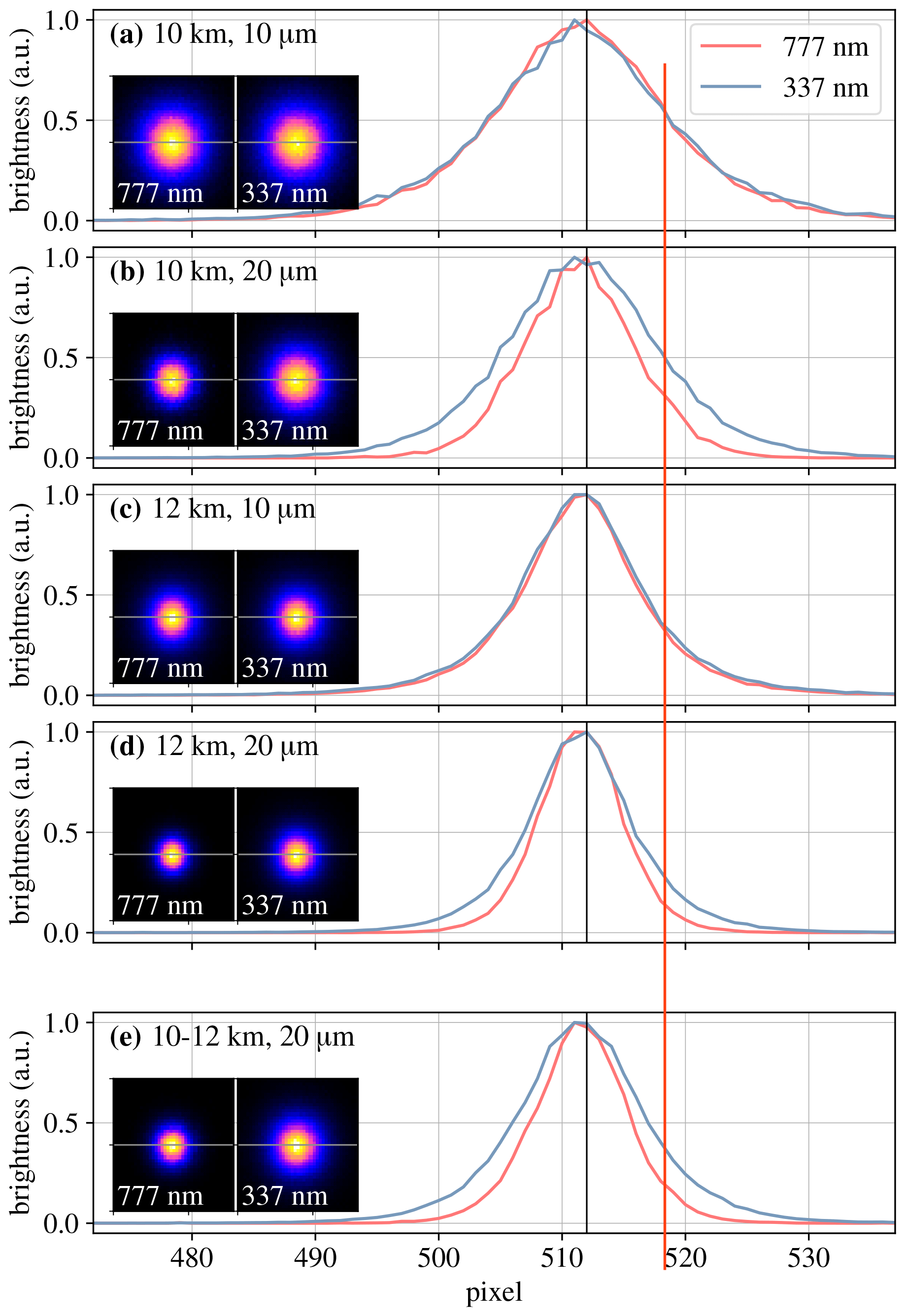
Figure 7 Simulated images of a cloud-scattered source at different wavelengths. Panels (a)–(d) show the integrated radiance produced by a point source at 10 or 12 km within a homogenous cylindrical 20 km radius cloud spanning altitudes between 5 and 15 km with a droplet radius of 10 or 20 µm and a droplet concentration of 100 cm⁻³. Panel (e) shows images of a vertically extended source from 10 to 12 km. All observations are performed in the nadir, and we plot the integrated radiances in a horizontal line crossing the sub-satellite point in each panel as well as the full images in each of insets at the left. To ease the comparison, all data and images are normalized to their peak value.

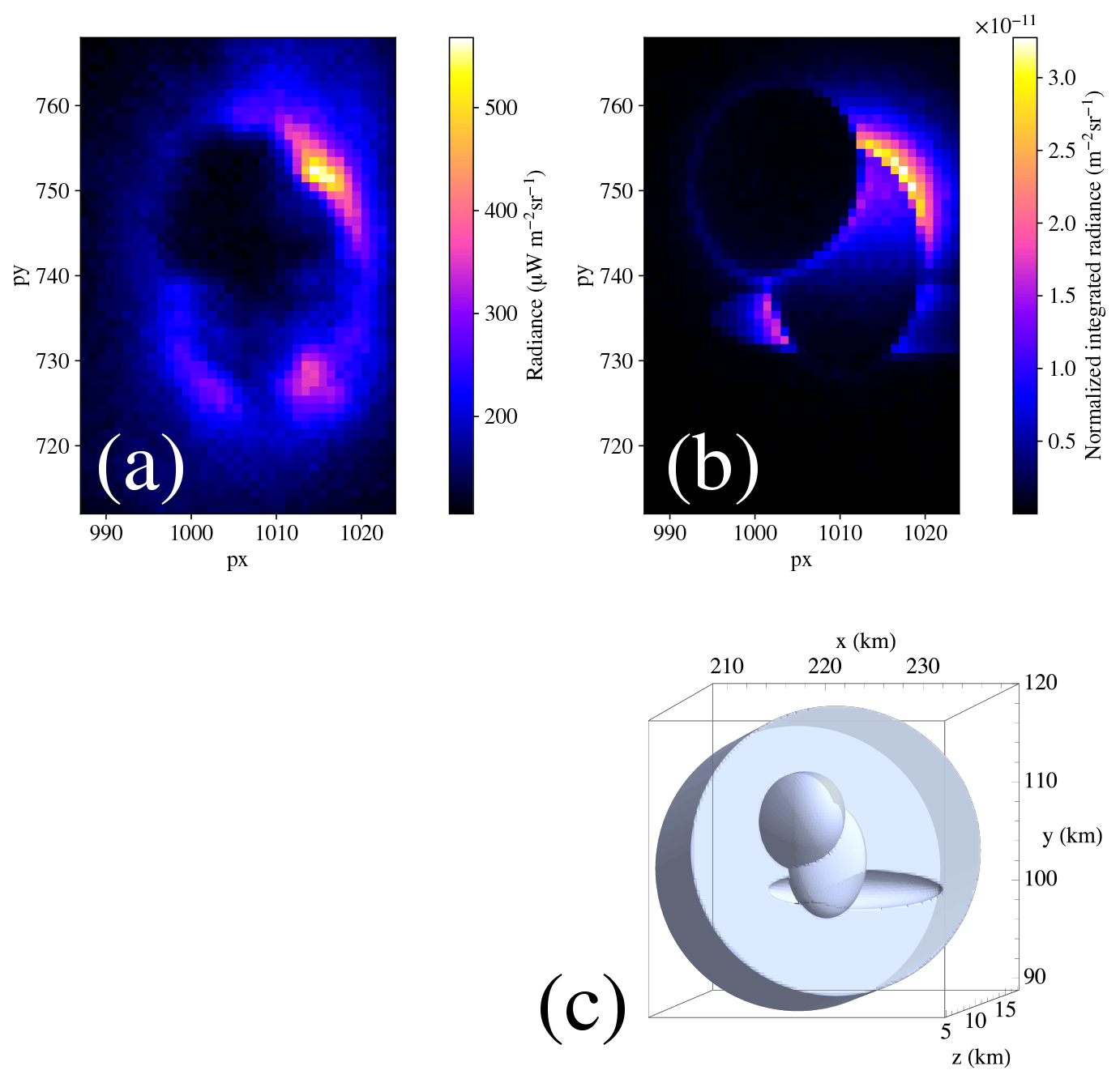
Figure 8 Comparison of a picture from the 337 nm filtered MMIA camera from ASIM (a) and a simulated observation from our Monte Carlo code (b) with the cloud geometry shown in panel (c). The MMIA picture was captured by the 337 nm filtered camera on 22 November 2019 at 08:43:05 at 4.45^∘ N, 77.50^∘ W.

Another feature of both pictures is the illumination of the lower cloud deck (2), partly due to light diffusing from inside the cloud and partly due to the reflection of light emerging from the turret's external boundary. A close look reveals a slight difference between the two wavelengths in the spatial distribution of this brightness, with the 337 nm illumination being somewhat more spread out. This difference will be analyzed in detail in the following section. The darkest areas are those not covered by the cloud, which is also somewhat contrary to our intuition.

One last feature of the simulated image is the weak, diffuse glow away from the brightest areas of the 337 nm picture (3), which is essentially absent in the 777 nm simulation. This glow results from Rayleigh scattering in the atmosphere above and around the cloud. Here, these image areas are 3 to 4 orders of magnitude dimmer than the brightest features.

3.5 Imaging at different wavelengths

Our next application is understanding differences in how a lightning source looks as it is imaged at different wavelengths. As we mentioned in the introduction, the MMIA module of ASIM contains cameras with wavelength filters at around 337 and 777 nm; thus, we restrict ourselves to these wavelengths.

Solving the Mie scattering problem shows that the extinction parameter (always close to 2) and the asymmetry parameter only weakly depend on the radiation wavelength. It is the single-scattering albedo (the absorption by cloud droplets) that dominates the differences between different wavelengths. Table 2 shows the different absorption properties of the cloud microphysical parameters that we have considered in our simulations. Remarkably, the different absorption rates are visible in a cloud-scattered image as a softer, more blurred image in the least absorbed band.

Table 2 Absorption of light of different wavelengths by clouds with droplet radii of 10 and 20 µm and a density of 100 cm⁻³. See the text for the definition of the single-scattering albedo ω₀ and expression (24) for the absorption time.

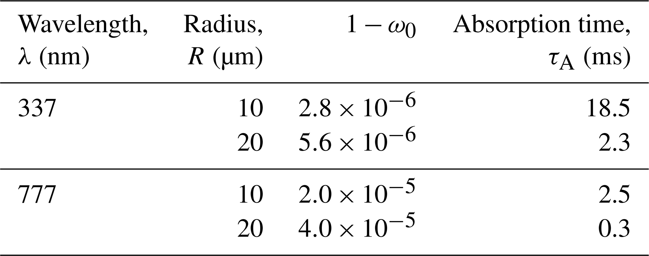
To illustrate this feature, we simulate observations of sources within a 20 km radius cylindrical cloud between an altitude of 5 and 15 km (the larger span of the cloud compared with other simulations limits the leakage of photons from the lower edge). The cloud is populated with a droplet density of 100 cm⁻³, and we test droplet radii of 10 and 20 µm to emphasize the role of absorption, with the latter value leading to much higher absorption rates. Figure 7a–d compare the outcomes of these simulations. We notice that when absorption is weaker, the emissions of a point source are more spread out and look more diffuse. The reason for this is that photons that travel radially spend more time inside the cloud and have a higher probability of being absorbed. This reduces the spread of the most absorbed radiation, which, in this case, is in the 777 nm band.

This effect is somewhat stronger if the light source extends vertically. This is shown in Fig. 7e, which contains results of a simulation similar to those in Fig. 7b and d (i.e., 20 µm droplets) but where the source is a vertical channel with a constant luminosity per unit length extending from an altitude of 10 to 12 km. In this case, we see that the difference between the two wavelengths is even more noticeable than in either Fig. 7b or d. The reason for this is that, due to a weaker absorption of the 337 nm band, we are capable of seeing emissions in this wavelength coming from deeper within the cloud and these create a wider image (Eq. 29 provides a quantitative estimate of this).

3.6 Interpretation of an MMIA observation

As a final application of the code, we analyze an actual observation recorded by the MMIA module of ASIM. We chose an event that took place on 22 November 2019 at 08:43:05 UTC at 4.45^∘ N, 77.50^∘ W (about 10 km off the Pacific coast of Colombia).

Figure 8a contains the image from MMIA's 337 nm filtered camera. There is a ring structure that suggests the effect of a cloud turret extending above a lower cloud surface. The cloud turret contains two differentiated regions, with the lower being somewhat brighter. Finally, the lower part of the ring surrounding the turret has two maxima to the left and right.

These considerations suggest that the discharge may have taken place below a cloud turret with two lobes and a slight depression in the cloud top to explain the two lower maxima. Therefore, we constructed the following cloud shape: the cloud base is a 15 km radius cylinder between an altitude of 5 and 12 km. From this cylinder, we subtract an ellipsoid with semi-axes $(\mathrm{4}\mathrm{km},\mathrm{6}\mathrm{km},\mathrm{2}\mathrm{km})$ and centered at $(\mathrm{2}\mathrm{km},-\mathrm{4}\mathrm{km},\mathrm{12}\mathrm{km})$ with respect to the ground point below the base center. The two lobes are represented by ellipsoids: the first one with semi-axes $(\mathrm{4}\mathrm{km},\mathrm{6}\mathrm{km},\mathrm{2}\mathrm{km})$ and centered at $(-\mathrm{1}\mathrm{km},-\mathrm{1}\mathrm{km},\mathrm{12}\mathrm{km})$ and the second with semi-axes $(\mathrm{4}\mathrm{km},\mathrm{5}\mathrm{km},\mathrm{5}\mathrm{km})$ and centered at $(-\mathrm{4}\mathrm{km},\mathrm{3}\mathrm{km},\mathrm{12}\mathrm{km})$. Moreover, the dark upper lobe in the MMIA image may indicate a strong absorption at higher altitudes, so we imposed an effective droplet radius that grows linearly from 10 µm at the lower boundary of the cloud (5 km) to 20 µm at the upper boundary of the tallest lobe (15 km). The droplet density is set to 100 cm⁻³ everywhere inside the cloud.

The implemented geometry is plotted in Fig. 8c, and the simulation results in Fig. 8b can be compared with the direct observation. We made no attempt to rigorously fit the geometry parameters to the observations, and, clearly, there are too many possible configurations that would produce similar observations to claim that the hypothesized shape really captures the reality of the cloud. The point of this exercise was rather to show the usefulness of the Monte Carlo model to test hypothesis about the cloud composition and configuration as well as to gain intuition about them.

4 Conclusions

We developed the CloudScat.jl code to assist in the interpretation of space-based observations of lightning-illuminated clouds. We were particularly interested in observations by the MMIA module of the ASIM instrument onboard the International Space Station, but we invite the broader research community to experiment with our code and adapt it to other observation platforms.

At present, the cloud microphysics in the code is somewhat oversimplified and does not compete in sophistication with radiative transfer models in other areas of the climate and weather research communities. Future work could address this shortcoming by combining our radiative transfer code with cloud physics models and with additional inputs from other Earth-observing spacecraft. This path, using a different code, has very recently been undertaken by Brunner and Bitzer (2019).

Currently the atmospheric electricity community regards the scattering of lightning-produced optical radiation by clouds as a hindrance that prevents a more detailed view of the lightning discharge. However, there is another point of view whereby lightning discharges are beacons that probe the cloud microphysics by allowing a deeper view into them. To realize this possibility, one needs, in addition to good space-borne detectors, reliable numerical codes to interpret the observations. It is our intention that our code serves in this role.

Appendix A: Implementation details

The code presented here is implemented in the Julia programming language. Although this language is gaining adoption in numerically intensive research areas, it is still less popular than more established languages such as Python, Fortran and C++. However, we considered it particularly suited for our application because it offers a large amount of flexibility with little or no performance overhead. This is visible in some aspects of our code that we wish to mention.

A significant feature of Julia is that each function is compiled at the time of first call with its code being specialized for the given argument types. That means that the compiler uses information contained in these types to optimize the output code.

We make use of this feature in the specification of the cloud composition, where we define different types for homogeneous and inhomogeneous clouds. For an inhomogeneous cloud, the code has to repeatedly call a function that probes the cloud composition at each collision location. In principle, one could particularize this to a homogeneous cloud by letting this function always return the same value; however, we would then needlessly call this function many times. This is avoided in Julia because even if the cloud composition is specified dynamically (i.e., at run time), the subsequent code is specialized depending on whether the cloud is homogeneous or not.

A similar benefit is obtained regarding the cloud geometry, which is defined as a complex structure of nested affine transforms and Boolean operations that act on different types of elementary shapes. We encode this structure into a data type and make it available to the compiler. In this case, to ensure that the code is fully specialized to the geometry structure, we employed another Julia feature, which is meta-programming, particularly generated functions. In these functions the code can be constructed dynamically according to the type of the function arguments. Thus, we dynamically build code tailored to the specific cloud geometry that is then compiled and fully optimized. This ensures the highest possible performance for each configuration.

These kind of optimizations are also available in other compiled languages like Fortran or C++; however, one loses the dynamical capability in those cases, leading to a slower development cycle and a poorer user experience.