Description and evaluation of a detailed gas-phase chemistry scheme in the TM5-MP global chemistry transport model (r112)

This work documents and evaluates the tropospheric gas-phase chemical mechanism MOGUNTIA in the three-dimensional chemistry transport model TM5-MP. Compared to the modified CB05 (mCB05) chemical mechanism previously used in the model, MOGUNTIA includes a detailed representation of the light hydrocarbons (C1–C4) and isoprene, along with a simplified chemistry representation of terpenes and aromatics. Another feature implemented in TM5-MP for this work is the use of the Rosenbrock solver in the chemistry code, which can replace the classical Euler backward integration method of the model. Global budgets of ozone (O₃), carbon monoxide (CO), hydroxyl radicals (OH), nitrogen oxides (NO_x), and volatile organic compounds (VOCs) are analyzed, and their mixing ratios are compared with a series of surface, aircraft, and satellite observations for the year 2006. Both mechanisms appear to be able to satisfactorily represent observed mixing ratios of important trace gases, with the MOGUNTIA chemistry configuration yielding lower biases than mCB05 compared to measurements in most of the cases. However, the two chemical mechanisms fail to reproduce the observed mixing ratios of light VOCs, indicating insufficient primary emission source strengths, oxidation that is too fast, and/or a low bias in the secondary contribution to C2–C3 organics via VOC atmospheric oxidation. Relative computational memory and time requirements of the different model configurations are also compared and discussed. Overall, the MOGUNTIA scheme simulates a large suite of oxygenated VOCs that are observed in the atmosphere at significant levels. This significantly expands the possible applications of TM5-MP.

1 Introduction

Chemistry transport models (CTMs) are tools to effectively study the temporal and spatial evolution of atmospheric species at regional and global scales, as well as to understand how the main physical and chemical processes in the troposphere (e.g., emissions, chemistry, transport, and deposition) influence air quality. Model investigations and analyses of the changes in important tropospheric pollutants, such as ozone (O₃) and carbon monoxide (CO), can further provide essential information about the oxidative capacity of the atmosphere and thus the lifetime of important climate gases like methane (CH₄). The oxidative capacity also controls the rate of formation and growth of aerosols by conversion of sulfur oxides into particulate sulfate (${\mathrm{SO}}_{\mathrm{4}}^{\mathrm{2}-}$) and volatile organic compounds (VOCs) into condensable organic matter that forms organic particles. Under certain tropospheric conditions (e.g., intense sunlight and high temperatures) the oxidation of VOCs in the presence of nitrogen oxides (NO_x≡ NO + NO₂) enhances the formation of secondary pollutants, such as O₃ (Crutzen, 1974; Derwent et al., 1996; Monks et al., 2009). VOCs and NO_x arise from both natural and anthropogenic emission sources. NO_x can be further converted into other chemical species such as HNO₃ and particulate nitrate (${\mathrm{NO}}_{\mathrm{3}}^{-}$) that together with ${\mathrm{SO}}_{\mathrm{4}}^{\mathrm{2}-}$ are key contributors to atmospheric acidity. The photochemical production of tropospheric O₃, a known toxic air pollutant that is transported over long distances, depends on the NO_x and VOC availability in a nonlinear manner (e.g., Seinfeld and Pandis, 2006). Under high-NO_x conditions, common in densely populated areas (i.e., VOC-limited regimes), O₃ production is inhibited and reductions in NO_x emissions can locally increase O₃. In contrast, in rural areas, O₃ production is more efficient, and NO_x emission reductions will decrease O₃ (i.e., NO_x-limited regimes). Thus, changes in emissions of NO_x and VOC may lead to nonlinear responses in ozone and the oxidation capacity of the troposphere. Overall, understanding the photochemical processes in the troposphere via robust model simulations is key to the development of effective abatement strategies for pollutants that affect both air quality and climate, as well as to the prediction of the future atmospheric composition.

The gas-phase photochemistry in the troposphere consists of numerous and complex reactions between odd oxygen (${\mathrm{O}}_x\equiv \mathrm{O}+{\mathrm{O}}_{\mathrm{3}}$) and NO_x, coupled to the oxidation of various VOCs (e.g., Atkinson, 2000; Atkinson et al., 2004). Several chemical mechanisms of varying complexity in the representation of VOC oxidation are currently included in state-of-the-art CTMs. One of the most explicit mechanisms ever built for the simulation of the tropospheric VOC oxidation cycles, the Master Chemical Mechanism (MCM v3), comprises more than 12 690 reactions, involving more than 4350 organic species, and about 46 associated inorganic reactions (Jenkin et al., 1997, 2003). Note that recent updates further include detailed aromatic hydrocarbon (Bloss et al., 2005) and isoprene oxidation (Jenkin et al., 2015) mechanisms. Since this level of chemical complexity is far beyond the computational resources potentially available for three-dimensional (3-D) global tropospheric CTMs, simplifications are required that retain the essential features of the chemistry. To this end, various chemical mechanisms of tropospheric chemistry have been developed with different levels of complexity, mainly involving reductions of the number of VOCs considered by lumping organic species into representative surrogates. For example, the Statewide Air Pollution Research Center mechanism (SAPRC-99) is a well-documented gas-phase chemical mechanism used in many CTMs, including a rather detailed representation of tropospheric VOC oxidation based on an evaluation against over 1700 experiments performed in different smog chambers (e.g., Carter, 1995, 2010). SAPRC-99 does not model the oxidation of each VOC individually as the MCM does, but it uses a molecular lumping approach to assign VOCs to a smaller number of reactive species. Other well-documented mechanisms often used in CTMs are the Regional Atmospheric Chemistry Mechanism (RACM; e.g., Geiger et al., 2003; Goliff et al., 2013; Stockwell et al., 1997) and the Model of Ozone and Related Chemical Tracers mechanism (MOZART; Emmons et al., 2010; Horowitz et al., 2003). A molecular lumping mechanism has also been developed and initially used in the Model of the Global Universal Tracer transport In the Atmosphere (MOGUNTIA) 3-D climatological CTM (e.g., Kanakidou and Crutzen, 1999; Poisson et al., 2000; Baboukas et al., 2000) and in box-model applications for field data interpretation (e.g., Poisson et al., 2001; Vrekoussis et al., 2006); the latter chemical mechanism was the starting point for the model development presented here.

A mechanism that has been extensively used in numerous chemistry and climate modeling studies is the Carbon Bond Mechanism (CBM). The CBM has several different versions with different levels of complexity (e.g., reaction rate constant updates, additions of inorganic reactions, and additions of organic species to better represent the respective species and radicals in the atmosphere), such as the CB4 (e.g., Gery et al., 1989; Houweling et al., 1998; Luecken et al., 2008), the CBM 2005 (CB05; e.g., Yarwood et al., 2005; Williams et al., 2013, 2017; Flemming et al., 2015) and the CBM-Z (Zaveri and Peters, 1999). The lumped-structure approach of the CBM has been extensively evaluated against chamber studies (e.g., Yarwood et al., 2005).

Several studies have focused on the impact of the chemical complexity of the gas-phase mechanism on tropospheric simulations. These studies indicate an inevitable compromise between model accuracy and computational efficiency (e.g., Cai et al., 2011; Gross and Stockwell, 2003; Luecken et al., 2008; Sander et al., 2019). Indeed, for a given atmospheric condition, even different versions of the same mechanism (e.g., the CBM family) may give significantly different results. For instance, the more explicit representation of VOCs in CB05 leads to a higher production of O₃ compared to the more lumped CB4, mainly due to a higher production of peroxy radicals, aldehydes, and organic peroxides (Saylor and Stein, 2012). A comparison of CB05 with RACM (Kim et al., 2009) revealed that the most considerable differences appeared in areas with significant biogenic emissions due to the more complex chemistry of aldehydes in the presence of anthropogenic alkenes and alkanes. Box-model comparisons between the MCM and various state-of-the-art simplified tropospheric chemistry schemes also indicated that the differences between the chemistry schemes can be rather significant under high VOC loadings (Emmerson and Evans, 2009). Thus, the choice of a gas-phase mechanism for a model may introduce uncertainties in predictions of regulated gas-phase pollutants (e.g., Knote et al., 2015). Computational restrictions, such as memory and computing time savings, are always a critical point to consider for large-scale 3-D simulations, especially when higher spatial resolutions are applied. On the other hand, the ability to validate the results of a particular chemical scheme in a global model can be significantly higher for the more extensive schemes that provide an explicit treatment of gases, such as in comparisons with satellite retrievals and in situ observations of a series of individual species.

In this work, a detailed and complete chemistry scheme is implemented in the global CTM TM5-MP, the massively parallel (MP) version of the Tracer Model version 5 (TM5), with the aim to investigate whether the consistent biases in important tropospheric tracers, such as O₃, CO, OH, NO_x, and light VOCs, found in previous works (e.g., Huijnen et al., 2010; van Noije et al., 2014; Williams et al., 2013, 2017) are sensitive to the chemistry scheme that is used. For this, we use the well-documented tropospheric gas-phase chemistry scheme MOGUNTIA (e.g., Myriokefalitakis et al., 2008, and references therein; along with recent updates) and benchmark its performance in TM5-MP. Section 2 provides a short description of the current model version, focusing on the new features implemented in the gas-phase chemistry and the chemistry integration method. In particular, we describe the implementation of the Kinetic PreProcessor (KPP) software (Damian et al., 2002; Sandu and Sander, 2006) in TM5-MP, which offers higher flexibility for testing, updating, and further developing the chemistry code in the model. Note that we are mostly focusing here on the performance of the new chemical scheme in comparison to the scheme previously included in the model, i.e., the modified CB05 (mCB05). This version of the model was introduced by Huijnen et al. (2010) and Williams et al. (2013) and further updated by Williams et al. (2017). In Sect. 3, the model's performance is analyzed for the different chemical configurations used for this study, and in Sect. 4 a detailed budget analysis of important gas-phase species is presented. Section 5 presents the evaluation of the different configurations of this work. The model's ability to reproduce the variability of important tropospheric species in both space and time is discussed, along with the associated uncertainties in atmospheric burdens and lifetimes. Finally, in Sect. 6 the main conclusions are presented, and some of the benefits and drawbacks of both chemical mechanisms are discussed, together with proposed directions for future model development.

2 Model description

2.1 General

The well-documented offline 3-D global CTM TM5 (Krol et al., 2005) is used for this study. Historically, the model has evolved from the original TM2 model (Heimann et al., 1988) via the TM3 model (Houweling et al., 1998; Tsigaridis and Kanakidou, 2003) to TM4 (van Noije et al., 2004; Myriokefalitakis et al., 2008) and TM5 (Krol et al., 2005; Huijnen et al., 2010; van Noije et al., 2014; Williams et al., 2017). In TM5-MP, the parallelization of the model has been redesigned, allowing for affordable global simulations at high resolution, i.e., $\mathrm{1}{}^{\circ }\times \mathrm{1}{}^{\circ }$ globally (Williams et al., 2017). Moreover, in this new MP version, the two-way zoom capability of TM5 is no longer available. All applications of TM5 share the same methods for model discretization and operator splitting (Krol et al., 2005), the treatment of the meteorological fields, and the mass-conserving tracer transport (Bregman et al., 2003). TM5-MP is driven by meteorological fields from the ECMWF ERA-Interim reanalysis (Dee et al., 2011) with an update frequency of 3 h. The advection scheme used is based on the slopes scheme (Russell and Lerner, 1981), and deep and shallow cumulus convection is parameterized according to Tiedtke (1989). The performance of the transport in the model has been evaluated by Peters et al. (2004) using sulfur hexafluoride simulations and by analyzing the vertical and horizontal distribution of radon (²²²Rn) (Koffi et al., 2016; Williams et al., 2017). More recently, global transport features, such as the transport times associated with interhemispheric transport, vertical mixing in the troposphere, transport to and in the stratosphere, and transport of air masses between the land and ocean, were evaluated via an intercomparison of six global transport models (Krol et al., 2018).

TM5-MP is primarily designed for simulation of the troposphere (i.e., no explicit stratospheric chemistry is considered in the model). To capture stratospheric ozone effects on actinic fluxes and to ensure realistic ozone stratosphere–troposphere exchange (STE), the overhead stratospheric profile is nudged to the ozone dataset provided for the Coupled Model Intercomparison Project phase 6 (CMIP6). The boundary conditions for CH₄, both in the lower troposphere and the stratosphere, are also based on the respective global mean value from the CMIP6 dataset (see also Sect. 2.4) to scale the monthly 2-D climatological fields as derived from HALOE measurements (Grooß and Russell, 2005), with the same nudging heights and relaxation times as for the case of stratospheric O₃. This approach is justified due to the relatively long lifetime of CH₄. Additionally, for HNO₃ and CO in the stratosphere monthly mean latitudinal climatologies derived from ODIN space-based observations are applied by prescribing the ratio of ${\mathrm{HNO}}_{\mathrm{3}}/{\mathrm{O}}_{\mathrm{3}}$ (Jégou et al., 2008; Urban et al., 2009) and $\mathrm{CO}/{\mathrm{O}}_{\mathrm{3}}$ (Dupuy et al., 2004), respectively. Note, however, that when we present the chemical budgets in the troposphere, a tropopause definition using the O₃ mixing ratio threshold of 150 ppb (e.g., Stevenson et al., 2006) is applied. Moreover, budget results using the 100 ppb O₃ mixing ratios (e.g., Lamarque et al., 2012) as a tropopause level in the model are also provided. For clarity, we note that, based on these threshold values, the different model configurations presented in this work (see Sect. 2.5) lead to identical tropopause heights.

The gas-phase chemistry of the TM5-MP model is supplemented with the in-cloud oxidation of SO₂ through aqueous-phase reactions with H₂O₂ and O₃ that depend on the acidity of the solution (Dentener and Crutzen, 1993). The heterogeneous conversion of N₂O₅ into HNO₃ on the available surface area of cloud droplets, cirrus particles, and hydrated sulfate aerosols is also accounted for. For cloud droplets, the number of droplets per unit volume is calculated using the liquid water content provided in the ECMWF meteorological data used by TM5-MP, assuming an effective droplet radius of 8 µm. For the heterogeneous conversion of N₂O₅ on hydrated sulfate particles, the approach of Dentener and Crutzen (1993) is employed using a global mean reaction probability (γ value) of 0.02 and 0.01 on water and ice surfaces, respectively. Heterogeneous conversions also consider the total reactive surface area density of aerosols, with contributions to accumulation-mode aerosol from sulfate, nitrate, and ammonium being calculated by the EQuilibrium Simplified Aerosol Model (EQSAM) approach (Metzger et al., 2002). The distribution of these aerosol species is calculated online and coupled to the gas-phase precursors NH₃, H₂SO₄, and HNO₃. Note that the aerosol microphysics module M7 (Vignati et al., 2004) is used in the model, as described in Aan de Brugh et al. (2011) and van Noije et al. (2014), along with recent updates on the inclusion of secondary organic aerosols. For N₂O₅, the uptake coefficient (γ) is considered as a function of temperature and relative humidity (Evans and Jacob, 2005), whilst for HO₂ and NO₃ radicals fixed γ values of 0.06 and 10⁻³, respectively, are adopted across all aerosol types (Jacob, 2000).

The model considers the wet removal of atmospheric species by liquid and ice precipitation by both in-cloud and below-cloud scavenging. The fraction of gases removed by precipitation depends on Henry's law (see Table S1 in the Supplement), together with the dissociation constants, temperature, and liquid or ice water content. In-cloud scavenging in stratiform precipitation considers an altitude-dependent precipitation formation rate (also describing the conversion of cloud water into rainwater). For convective precipitation, highly soluble gases are assumed to be scavenged entirely in the vigorous convective updrafts producing rainfall rates of > 1 mm h⁻¹. Removal is exponentially scaled down for lower rainfall rates. For the dry deposition, the removal is calculated online in the model based on a series of surface and atmospheric resistances on a $\mathrm{1}{}^{\circ }\times \mathrm{1}{}^{\circ }$ spatial resolution (Wesely, 1989; Ganzeveld and Lelieveld, 1995; Ganzeveld et al., 1998). Overall, the calculated deposition velocities show both seasonal and diurnal cycles since they are calculated using 3-hourly meteorological and surface parameters based on the uptake resistances for vegetation (in-canopy aerodynamic, soil, and leaf resistance), soil, water, snow, and ice (see Table S2). A more detailed description of dry and wet deposition schemes for the removal of gases can be found in de Bruine et al. (2018).

2.2 Gas-phase chemistry

2.2.1 The original MOGUNTIA chemical scheme

The new chemical mechanism that has been implemented in TM5-MP for this study was originally developed for box (Poisson et al., 2001) and global (Kanakidou and Crutzen, 1999; Poisson et al., 2000) modeling studies, and it was initially coupled to the global 3-D CTM MOGUNTIA (Zimmermann, 1988). Since then, the scheme has been continuously updated for box modeling, coupled to the global TM4 model, and applied in numerous studies (e.g., Tsigaridis and Kanakidou, 2002; Gros et al., 2002; Myriokefalitakis et al., 2008; Daskalakis et al., 2015).

The MOGUNTIA chemical scheme employs a rather detailed oxidation scheme of light alkanes (CH₄, C₂H₆, and C₃H₈), light alkenes (C₂H₄ and C₃H₆), acetylene (C₂H₂), and isoprene (C₅H₈). Acetaldehyde (CH₃CHO), glyoxal (GLY; CHOCHO), glycolaldehyde (GLYAL; HOCH₂CHO), methylglyoxal (MGLY; CH₃C(O)CHO), and acetone (CH₃COCH₃) are also explicitly treated in the mechanism. The oxidation pathways of methacrolein (MACR; CH₃(CH₂)CH=O) and methylvinyl ketone (MVK; CH₃C(O)CH=CH₂) are also considered, together with the formation of formic (HCOOH) and acetic acid (CH₃COOH). Higher VOCs (i.e., C_n > 4), besides isoprene, are represented in the mechanism by the surrogate species n-butane (n-C₄H₁₀), motivated by the similar O_x and hydrogen oxides (HO_x) yields per oxidized carbon atom (see, e.g., Poisson et al., 2000; Stavrakou et al., 2009a). The second-generation oxidation products of higher hydrocarbons of biogenic origin (such as terpenes) and aromatics are also considered to follow the gas-phase oxidation pathways of the respective isoprene and surrogate n-C₄H₁₀ oxidation species.

The reactions of peroxy radicals (RO₂) with hydrogen peroxide (HO₂), methyl peroxide (CH₃O₂), and NO lead to organic hydroperoxides (ROOH), carbonyls, and organic nitrates, respectively. ROOH is removed by photolysis and reaction with OH. The addition of NO to the formed RO₂ radicals leads to alkyl nitrates (RONO₂), which are much longer-lived than NO_x. RONO₂ can thus be transported over longer distances than NO_x and serve as a sink for NO_x in high-NO_x regimes and as a source for NO_x in low-NO_x regimes. The RONO₂ compounds explicitly considered in this study are identified by R=CH₃, C₂H₅, C₃H₇, C₄H₉, HOC₂H₄O, and C₅H₈(OH), i.e., the first-generation product of isoprene oxidation. Additionally, the reactions of the acyl peroxy radicals (RC(O)O₂) with NO₂ produce peroxyacyl nitrates (RC(O)O₂NO₂), in particular peroxyacetyl nitrate (PAN; R=CH₃), which is the most abundant organic nitrate observed in the troposphere and the only species of this group that is considered here. Thermal decomposition is dominant for peroxyacyl nitrates, while it is negligible for alkyl nitrates. NO₃ radical reactions with aldehydes, alcohols, n-C₄H₁₀, dimethylsulfide (DMS), and unsaturated hydrocarbons are also considered. A more detailed description of the chemical scheme used for this study can be found in Poisson et al. (2000) and Myriokefalitakis et al. (2008).

2.2.2 Updates of the MOGUNTIA chemical mechanism

Several updates have been applied to the original MOGUNTIA chemical scheme with respect to the previous implementations (e.g., Poisson et al., 2000; Myriokefalitakis et al., 2008). These updates include reactions of major hydrocarbons, their rate constants, and oxidation pathways. Concerning the terpene chemistry, we consider one lumped monoterpene species (C₁₀H₁₆) for all terpenes (assuming a 50 : 50 α- : β-pinene distribution), in contrast to the consideration of the explicit oxidation of α- and β-pinene as performed in the previous implementations of the MOGUNTIA scheme (e.g., Myriokefalitakis et al., 2008, 2010). Thus, monoterpenes represent all terpenes and terpenoid species here. Likewise, toluene is used to represent all aromatics replacing benzene, xylene, and toluene used previously (Myriokefalitakis et al., 2008, 2010). Besides these compounds, toluene is also used to represent trimethyl-benzenes and higher aromatics. Moreover, for this work the coupling of the gas-phase chemistry with the aqueous-phase oxidation scheme of SO₂, as well as the gas-phase oxidation of dimethyl sulfide (DMS), methyl sulfonic acid (MSA), and ammonia (NH₃), follows the oxidation scheme outlined by Williams et al. (2013), which is slightly simpler compared to the MOGUNTIA scheme used in previous studies (e.g., Myriokefalitakis et al., 2010). Note that the lumping mentioned above, and the simplifications implemented here, aim at limiting the number of species without degrading the general performance of the chemical scheme for global-scale tropospheric chemistry.

Isoprene (2-methyl-1,3-butadiene; ISOP) oxidation has been extended with the production of isoprene epoxydiols (IEPOXs) and hydroperoxyaldehydes (HPALDs), as well as the HO_x recycling mechanism under low-NO_x conditions (Paulot et al., 2009; Peeters and Müller, 2010; Crounse et al., 2011; Browne et al., 2014). The latter species replaces the lumped second-generation oxidation product considered in previous implementations of the MOGUNTIA mechanism (Poisson et al., 2000; Myriokefalitakis et al., 2008). The oxidation of isoprene by the OH radical leads to the formation of several isomers of an unsaturated hydroxy hydroperoxide. In the presence of NO_x, this leads to the formation of carbonyl compounds. However, under low-NO_x conditions, the major product from unsaturated hydroxy hydroperoxide oxidation is IEPOX (i.e., cis- and trans-isomers). The organic peroxy radicals formed from OH oxidation of isoprene can react with either (1) HO₂ to form hydroperoxides or (2) NO to form hydroxynitrates, formaldehyde (HCHO), MVK, MACR and HO₂ (e.g., Paulot et al., 2009), or hydroperoxyenals (HPALDs). The latter are produced by the isomerization of the initial isoprene organic hydroperoxy radicals followed by reaction with O₂ and other oxidized products (Peeters et al., 2009; Peeters and Müller, 2010). Under HO₂-dominated conditions, the main products are unsaturated hydroperoxides (all possible isomers referred to as ISOPOOH; see Table 2). The fate of isoprene peroxy radicals is highly dependent on the mixing ratios of HO₂, NO, organic peroxy radicals, and the local meteorological conditions that affect thermal and photochemical reaction rates and wet and dry removal. Subsequent reactions of ISOPOOH with OH produce epoxydiols (cis- and trans-isomers referred to as IEPOXs) and regenerate OH radicals (Paulot et al., 2009). Moreover, the isoprene peroxy radical 1,6-H-shift isomerizations (Peeters et al., 2014; Peeters and Müller, 2010) lead to the formation of photolabile C5-hydroperoxyaldehydes (i.e., all possible isomers referred to as HPALDs; see Table 1). Overall, these additions to the chemistry scheme are expected to provide a better representation of OH regeneration during isoprene oxidation (e.g., Browne et al., 2014) compared to the previous implementation of the MOGUNTIA mechanism.

Table 1 Photolysis reactions (J) in the MOGUNTIA chemistry scheme.

^* The reaction products O₂, H₂, and H₂O are not shown. ¹ http://iupac.pole-ether.fr (last access: 20 August 2019)
² Atkinson (1997): $R_{\mathrm{1}}=\mathrm{2.7}\times {\mathrm{10}}^{\mathrm{14}}\exp (-\mathrm{6350}/T)$; $R_{\mathrm{2}}=\mathrm{6.3}\times {\mathrm{10}}^{-\mathrm{14}}\exp (-\mathrm{550}/T)$; $f=R_{\mathrm{1}}/(R_{\mathrm{1}}+R_{\mathrm{2}}\times [{\mathrm{O}}_{\mathrm{2}}\left]\right)$.
³ J_ORGN is calculated based on average σ values for 1-C₄H₉ONO₂ and 2-C₄H₉ONO₂ as described in Williams et al. (2012).
⁴ Browne et al. (2014). ⁵ Peeters and Müller (2010).

Table 2 Thermal reactions (K) in the MOGUNTIA chemistry scheme.

^* The reaction products O₂, H₂, and H₂O are not shown.
¹ The chemical kinetic data and mechanistic information were taken from the website of the IUPAC Task Group on Atmospheric Chemical Kinetic Data Evaluation: http://iupac.pole-ether.fr/ (last access: 20 August 2019).
² The chemical kinetic data and mechanistic information were taken from the website of the NASA Panel for Data Evaluation (Evaluation No. 18, JPL Publication 15-10; http://jpldataeval.jpl.nasa.gov, last access: 20 August 2019).
³ The chemistry mechanistic information was taken from the Master Chemical Mechanism (MCM v3.3.1) – for nonaromatic schemes: Jenkin et al. (1997); Saunders et al. (2003); for the isoprene scheme: Jenkin et al. (2015); for aromatic schemes: Jenkin et al. (2003); Bloss et al. (2005); via the website http://mcm.leeds.ac.uk/MCM (last access: 20 August 2019).
⁴ Atkinson (1997): $R_{\mathrm{1}}=\mathrm{2.7}\times {\mathrm{10}}^{\mathrm{14}}\exp (-\mathrm{6350}/T)$; $R_{\mathrm{2}}=\mathrm{6.3}\times {\mathrm{10}}^{-\mathrm{14}}\exp (-\mathrm{550}/T)$; $f=R_{\mathrm{1}}/(R_{\mathrm{1}}+R_{\mathrm{2}}\times [{\mathrm{O}}_{\mathrm{2}}\left]\right)$; $R_{\mathrm{1}}=\mathrm{1.94}\times {\mathrm{10}}^{-\mathrm{22}}\left[\text{AIR}\right]\exp (\mathrm{0.972}\times N_{\text{c}})$; $R_{\mathrm{2}}=\mathrm{0.826}\times (T/\mathrm{300}{)}^{-\mathrm{8.1}}$; $A=\mathrm{1}/(\mathrm{1}+{\log }_{\mathrm{10}}(R_{\mathrm{1}}/R_{\mathrm{2}}{)}^{\mathrm{2}})$; $\text{RTC}\left(N_{\text{c}}\right)P=\mathrm{0.4}\times R_{\mathrm{1}}/(\mathrm{1}+R_{\mathrm{1}}/R_{\mathrm{2}}){\mathrm{0.411}}^A$; $\text{RTC}\left(N_{\text{c}}\right)S=R\mathrm{1}/(\mathrm{1}+R_{\mathrm{1}}/R_{\mathrm{2}}){\mathrm{0.411}}^A$,
where N_c is the number of carbons (i.e., 1–5).
⁵ Orlando et al. (1992); Poisson et al. (2000); ⁶ Peeters and Müller (2010); ⁷ Crounse et al. (2011); ⁸ Paulot et al. (2009); ⁹ Browne et al. (2014); ¹⁰ Average of α- and β-pinene; ¹¹ A1, A2, and A3 represent the relative contributions of ortho-, meta-, and para-xylene (A1), toluene (A2), and benzene (A3); roughly 0.4, 0.6, and 0.4, respectively, for the year 2006.
¹² Average of ortho-, meta-, and para-isomers of xylene.

The MOGUNTIA chemistry scheme is in line with the VOC oxidation pathways as proposed by the Master Chemistry Mechanism (MCM v3.3.1) (e.g., Bloss et al., 2005; Saunders et al., 2003). The thermal and pressure-dependent reaction rate coefficients of the MOGUNTIA chemical mechanism are taken (when available) from the IUPAC kinetic data evaluation (Atkinson et al., 2004; Wallington et al., 2018) and supplemented with reaction rates based on recommendations given by the JPL (Burkholder et al., 2015). Photolysis frequencies needed to drive MOGUNTIA are taken from the IUPAC database (Atkinson, 1997; Atkinson et al., 2004) along with the updates from MCM v3.3.1 (Bloss et al., 2005; Jenkin et al., 1997, 2003, 2015; Saunders et al., 2003). Note that the model calculates the photolysis frequencies online as described in Williams et al. (2012). Comprehensive lists of all photochemical and thermal kinetic reactions included in the current MOGUNTIA chemical scheme are presented in Tables 1 and 2, respectively.

2.3 The chemical solver

The KPP version 2.2.3 (Damian et al., 2002; Sandu and Sander, 2006) is employed here to generate Fortran 90 code for the numerical integration of the gas-phase chemical mechanisms. An important advantage of this approach is that the implementation of a KPP-generated code in the model is less prone to errors than coding the mechanism manually. Upon the translation of the chemistry mechanisms (e.g., species, reactions, rate coefficients) from the KPP language into a Fortran 90 code, a model driver was developed to arrange the respective couplings to TM5-MP. Minor changes, however, were needed in the KPP code to deal with TM5-MP I/O requirements. The photolysis and thermal reactions are not calculated in KPP but explicitly calculated by the respective modules of TM5-MP and then directly provided to the aforementioned chemistry driver. To this end, only the integration method has been updated in the model, replacing the default hand-coded chemical solver setup. Moreover, the NO emission rates (and the dry deposition terms of all deposited species) are imported to KPP through the application of appropriate production (and loss) rates, as previously done for the Euler backward iterative (EBI) solver, owing mainly to the numerical stiffness of the $\mathrm{NO}-{\mathrm{NO}}_{\mathrm{2}}-{\mathrm{O}}_{\mathrm{3}}$ photostationary state and their fast interactions (see, e.g., Huijnen et al., 2010). In this study, the Rosenbrock solver is used as the numerical integrator (Sander et al., 2019). The Rosenbrock solver has been shown to be robust and capable of integrating very stiff sets of equations (Sander et al., 2011). For all previous versions of the model, the EBI solver (Hertel et al., 1993) was used. This holds for the modified CB4 (Houweling et al., 1998), mCB05 (Williams et al., 2013), and MOGUNTIA (Myriokefalitakis et al., 2008) mechanisms. Note, however, that EBI was originally designed for the CB4 mechanism (Gery et al., 1989), and it is a rather fast and robust solver suitable for use in large-scale atmospheric models that incorporate operator splitting (Huang and Chang, 2001).

The favorable comparison of the Rosenbrock solver against other widely used methods, such as FACSIMILE (Curtis and Sweetenham, 1987), has already been described in the literature (e.g., Sander et al., 2005). Focusing specifically on the comparison of a series of Rosenbrock solvers to EBI, Sandu et al. (1997) concluded that, although EBI appears robust, especially when it is used with a relatively large time step, the Rosenbrock methods with variable time steps are significantly more accurate and clearly superior for accuracies in the range of 1 % compared to EBI for a range of species examined. The main aim of this study is not to compare the two chemistry solvers (i.e., the Rosenbrock vs. the EBI). Instead, we present model simulations using the Rosenbrock solver as produced by KPP for the mCB05 scheme (see Sect. 2.5) to isolate the impact of the solver on various species mixing ratios in this work.

2.4 Emission setup

For the present study, emissions from anthropogenic activities, including aircraft emissions (Hoesly et al., 2018) and biomass burning (speciated for agricultural waste burning, deforestation fires, boreal forest fires, peat fires, savanna fires, and temperate forest fires; van Marle et al., 2017), are adopted from the sectoral and gridded historical inventories as developed for CMIP6 (Eyring et al., 2016). In more detail, anthropogenic and biomass burning emissions of CO, NO_x, black carbon aerosol (BC), particulate organic carbon (OC), sulfur dioxide and sulfates (SO_x), and speciated non-methane volatile organic compounds (NMVOCs) are considered, such as emissions of ethane (C₂H₆), methanol (CH₃OH), ethanol (C₂H₅OH), propane (C₃H₈), acetylene (C₂H₂), ethane (C₂H₄), propene (C₃H₆), isoprene (C₅H₈), monoterpenes (C₁₀H₁₆), benzene (C₆H₆), toluene (C₇H₈), xylene (C₈H₁₀) and other aromatics, higher alkenes, higher alkanes, HCHO, acetaldehyde (CH₃CHO), acetone (CH₃COCH₃), dimethylsulfide (DMS; C₂H₆S), formic acid (HCOOH), acetic acid (CH₃COOH), methyl ethyl ketone (MEK; CH₃CH₂COCH₃), methylglyoxal (MGLY; CH₃C(O)CHO), and hydroxyacetaldehyde (HOCH₂CHO). Note that all biomass burning emissions (open forest and grassland fires) are vertically distributed in the model over latitude-dependent injection heights, i.e., for tropical (30^∘ S–30^∘ N), temperate (30–60^∘ S–N), and high-latitude (60–90^∘ S–N) forest fires (see the Appendix in van Noije et al., 2014).

Biogenic emissions from vegetation include isoprene, terpenes and other volatile organic compounds, and CO. Emissions are based on the Model of Emissions of Gases and Aerosols from Nature (MEGAN) version 2.1 (Sindelarova et al., 2014). Isoprene and terpene emissions are distributed over the first ∼ 50 m from the surface and a diurnal cycle is imposed. The biogenic emissions from soils include NO_x (Yienger and Levy, 1995), NH₃ and terrestrial DMS emissions from soils and vegetation (Spiro et al., 1992). Oceanic emissions of CO and NMVOCs come from the POET database (Granier et al., 2005), oceanic emissions of NH₃ from Bouwman et al. (1997), and the DMS oceanic emissions are calculated online using the seawater concentration climatology from Lana et al. (2011). The NO_x production by lightning is parameterized based on convective precipitation fields (Meijer et al., 2001), and the SO_x fluxes from continuously emitting volcanoes are taken from Andres and Kasgnoc (1998). Note that we focus below on the more detailed representation of emissions as used for the MOGUNTIA chemical scheme. Emissions of other tropospheric species in the gas and the particulate phase are described in detail in previous studies (e.g., van Noije et al., 2014).

The MOGUNTIA chemical scheme considers direct emissions of CO, CH₄, HCHO, HCOOH, CH₃OH, C₂H₆, C₂H₄, C₂H₂, CH₃CHO, CH₃COOH, C₂H₅OH, HOCH₂CHO, CHOCHO, C₃H₈, C₃H₆, n−C₄H₁₀, MEK, C₅H₈, C₁₀H₁₆, and C₇H₈, as well as NO_x, NH₃, DMS, and SO_x. Butanes, pentanes, hexanes, and higher alkane emissions are summed up into the lumped n-C₄H₁₀ species, which represents the alkanes containing four or more carbon atoms. For reactivity purposes, higher alkene emissions containing four or more carbon atoms (butenes and higher alkenes) are accounted for as equivalent C₃H₆ emissions. Higher ketones (i.e., except for acetone) from open biomass burning emissions are represented as MEK. Emissions of benzene (C₆H₆), toluene (C₇H₈), xylene (C₈H₁₀), trimethyl-benzenes, and other higher aromatics and VOCs are represented by toluene as in the MOZART mechanism (Emmons et al., 2010). Note that when VOC emissions are assigned to a lumped species, adjustments are made to preserve their atmospheric reactivity (see also notes in Tables 1 and 2).

The explicit parameterization of VOC species in the MOGUNTIA chemical scheme requires emissions that are not routinely included in available emission databases. Direct biofuel and biomass burning emissions of light carbonyls have been reported in several studies (e.g., Christian et al., 2003; Fu et al., 2008; Hays et al., 2002), and these represent a significant contribution to the VOC budget (e.g., Fu et al., 2008; Myriokefalitakis et al., 2008; Stavrakou et al., 2009b, a; Vrekoussis et al., 2009). For this reason, emissions from biofuel use of 1.4, 2.4, and 1.6 Tg yr⁻¹ are considered for GLYAL, GLY, and MGLY, respectively. For the biomass burning sector, we use global emissions of GLYAL and GLY of 4.3 and 5.2 Tg yr⁻¹, respectively. We base these emission rates on the HCHO emissions distribution because mass emission rates of low-molecular-weight carbonyls, such as HCHO and GLY (e.g., Hays et al., 2002), are highly correlated. Global emissions of roughly 1.4 Tg yr⁻¹ (Emmons et al., 2010) are also considered for MEK, accounting for anthropogenic emissions (Rodigast et al., 2016) such as domestic burning and solvent use (e.g., Ware, 1988). For all other carbonyls, primary anthropogenic emissions are considered negligible (e.g., Fu et al., 2008). A list of the global annual emission strengths considered for the MOGUNTIA chemical configuration is presented in Table 3. For completeness, we note that primary aerosol emissions of OC, BC, sea salt, and dust are also considered in the model, with sea salt and dust emissions calculated online. A more detailed description of the gas and aerosol emissions used in the model will be presented in van Noije et al. (2020).

Table 3 Global annual emissions of trace gases used for the MOGUNTIA chemistry scheme in TM5-MP for the year 2006 (Tg yr⁻¹ unless specified otherwise).

^a Including aircraft emissions; ^b Tg N yr⁻¹; ^c NO_x production from lightning; ^d SO₂ from volcanoes.

2.5 Simulations

We will present the analysis of TM5-MP simulations with the mCB05 and MOGUNTIA chemical mechanisms for the year 2006, which has been the chosen year of previous benchmarking studies (Huijnen et al., 2010; Williams et al., 2013, 2017). All simulations have been performed at $\mathrm{1}{}^{\circ }\times \mathrm{1}{}^{\circ }$ horizontal resolution (e.g., Williams et al., 2017) with 34 vertical layers and use a 1-year spin-up (i.e., for the year 2005). The same emission datasets have been used in all simulations, albeit with higher speciation for the MOGUNTIA chemical scheme. Overall, two simulations have been performed for the mCB05 configuration: one employing the EBI solver (mCB05(EBI)) and one employing the KPP-generated Rosenbrock solver (mCB05(KPP)). This approach isolates differences that are caused solely by the applied chemistry solver. By comparing MOGUNTIA generated by KPP with mCB05(KPP), the differences due to the chemistry setup in the model are isolated.

3 Model performance

Concerning the TM5-MP performance, simulations performed on the ECMWF CRAY XC40 high-performance computer facility using 360 cores indicate that the coupling of KPP software alone increases the time spent in chemistry by ∼ 59 % and overall slows down the code by ∼ 18 % compared to the (hand-coded) EBI version for the mCB05 mechanism. As expected, the coupling of the MOGUNTIA atmospheric chemistry scheme further increases the model runtime. MOGUNTIA uses 100 transported and 28 non-transported tracers, numbers that are significantly larger than the mCB05 configuration (i.e., 69 transported and 21 non-transported tracers). As a result, time spent to transport the tracers increases by ∼ 43 %, and the chemistry calculations slow down by ∼ 55 %. Altogether, the newly coupled MOGUNTIA chemistry scheme in TM5-MP is computationally ∼ 27 % more expensive than the mCB05(EBI) configuration. Overall, the mCB05(EBI), mCB05(KPP), and MOGUNTIA configurations simulate 0.73, 0.60, and 0.44 years per day of simulation time, respectively (Table S3a). Note that an additional series of simulations with 450 cores leads to only marginal changes (Table S3b). Finally, the runtime values for the different model configurations presented here are highly hardware-dependent, owing mainly to the large I/O component associated with reading the meteorological fields.

4 Comparison of budgets and tropospheric mixing ratios

4.1 Ozone (O₃)

Table 4 presents a detailed description of the chemical budget of tropospheric ozone, as calculated by the TM5-MP model, for the three chemical configurations. Following Stevenson et al. (2006), chemical production of ozone is derived from all reactions that convert NO to NO₂, since NO₂ is rapidly photodissociated and forms O₃, i.e.,

$$\begin{array}{}\text{(R1)}& {\displaystyle }& {\displaystyle }\mathrm{NO}+{\mathrm{HO}}_{\mathrm{2}}\to {\mathrm{NO}}_{\mathrm{2}}+\mathrm{OH},\text{(R2)}& {\displaystyle }& {\displaystyle }\mathrm{NO}+{\mathrm{RO}}_{\mathrm{2}}\to {\mathrm{NO}}_{\mathrm{2}}+\mathrm{RO},\end{array}$$

where RO₂ represents all the major organic peroxy radicals of the corresponding chemistry mechanism used in the model. For the MOGUNTIA scheme RO₂ includes CH₃O₂, C₂H₅O₂, HYEO₂, n-C₃H₇O₂, i-C₃H₇O₂, ACO₂, HYPO₂, n-C₄H₉O, MEKO₂, ISOPO₂, IEPOXO₂, MVKO₂, MACRO₂, TERO₂, and AROO₂ radicals. For mCB05, RO₂ includes the CH₃O₂ radical and XO₂ (i.e., the operator for the NO to NO₂ conversion, which represents all lumped alkyl-peroxy radicals in mCB05; see Williams et al., 2017, and Yarwood et al., 2005).

Table 4 Tropospheric budgets and burden (Tg(O₃)) of O₃ for the year 2006 (Tg(O₃) yr⁻¹) using the 150 ppb O₃ mixing ratio to define the tropopause level. In parentheses, the relative differences using the 100 ppb O₃ mixing ratios are also presented, calculated with reference to the 150 ppb O₃ tropopause level definition.

^* Sum of the deposition and the tropospheric chemical loss minus the production.

The chemical O₃ loss is derived as the sum of the

1. O₃ photolysis to O(¹D), i.e.,

   $$\begin{array}{}\text{(R3)}& {\displaystyle }{\mathrm{O}}_{\mathrm{3}}+h\mathit{\nu }\to \mathrm{O}{(}^{\mathrm{1}}\mathrm{D})+{\mathrm{O}}_{\mathrm{2}},\end{array}$$

   followed by reaction with H₂O to form OH, i.e.,

   $$\begin{array}{}\text{(R4)}& {\displaystyle }\mathrm{O}{(}^{\mathrm{1}}\mathrm{D})+{\mathrm{H}}_{\mathrm{2}}\mathrm{O}\to \mathrm{2}\mathrm{OH},\end{array}$$

2. O₃ destruction by HO₂ and OH catalytic cycles, i.e.,

   $$\begin{array}{}\text{(R5)}& {\displaystyle }& {\displaystyle }{\mathrm{O}}_{\mathrm{3}}+{\mathrm{HO}}_{\mathrm{2}}\to \mathrm{OH}+\mathrm{2}{\mathrm{O}}_{\mathrm{2}},\text{(R6)}& {\displaystyle }& {\displaystyle }{\mathrm{O}}_{\mathrm{3}}+\mathrm{OH}\to {\mathrm{HO}}_{\mathrm{2}}+{\mathrm{O}}_{\mathrm{2}},\end{array}$$

   and

3. reactions of O₃ with unsaturated VOCs. Chemical loss calculations exclude contributions from HNO₃, NO₃, N₂O₅, and other fast cycles between ozone-related species, as proposed by Stevenson et al. (2006).

For the MOGUNTIA scheme, the tropospheric chemical production is calculated to be 5709 Tg yr⁻¹, which is only ∼ 10 Tg yr⁻¹ smaller compared to the mCB05(KPP) configuration. Chemical destruction in the troposphere is similar in the MOGUNTIA and mCB05(KPP) chemistry configurations (Table 4). The use of EBI compared to the Rosenbrock solver decreases the O₃ chemical production (5719 vs. 5589 Tg yr⁻¹) and destruction (5216 vs. 5192 Tg yr⁻¹) terms in the troposphere (Table 4). Besides some expected differences due to the behavior of the two solvers, the calculated differences may also be partly attributed to the mass fixer for NO_Y (i.e., the sum of NO, NO₂, NO₃, HNO₃, HNO₄, 2×N₂O₅, PAN, and the organic nitrate compounds) that is applied in the mCB05(EBI) configuration to ensure no artificial loss of nitrogen. NO_Y fixing occurs mainly over highly polluted regions with active NO_x photochemistry to improve the accuracy of the EBI solver.

Focusing on the impact of the stratosphere on the tropospheric O₃ budget, the net STE flux of O₃ for the MOGUNTIA configuration is somewhat lower (∼ 1 %) than for mCB05(KPP). Considering that all configurations use the same stratospheric ozone relaxation parameterization, this difference can only be attributed to the chemical schemes. Note that the global STE of O₃ is defined by simply considering the chemical production and loss budget terms, as proposed by Stevenson et al. (2006). The differences in the O₃ stratospheric inflow budgets for the three chemistry configurations (Table 4) do not imply that the tropospheric chemistry impacts O₃ transport from the stratosphere, but rather that the global budget is closed by an inferred stratospheric input term. Thus, the higher net chemical production of O₃ in the troposphere implies a lower contribution from the stratosphere to the troposphere for roughly the same deposition losses. The calculated net influx from the stratosphere for the MOGUNTIA configuration (∼ 424 Tg yr⁻¹) remains within 1 standard deviation of a multi-model mean (552±168 Tg yr⁻¹), as reported by both Stevenson et al. (2006) and Young et al. (2013). MOGUNTIA calculations are also in line with estimates (∼ 400 Tg yr⁻¹) based on observations (Hsu, 2005; Olsen, 2004), although they are higher compared to the 306 Tg yr⁻¹ calculated by an earlier version of the TM5 model driven by the same meteorological fields (van Noije et al., 2014). Overall, compared to the mCB05(EBI) simulation, the lower net stratosphere–troposphere exchange flux simulated in the MOGUNTIA configuration brings the model results closer to the current best estimates of the net STE.

The MOGUNTIA configuration also results in a reduction of roughly 2 % in the tropospheric O₃ burden compared to both mCB05 configurations. No significant change in the O₃ lifetime in the troposphere (i.e., 22.3–22.8 d) is found, and the calculated lifetimes remain close to other model estimates of ∼ 22 d (Stevenson et al., 2006; Young et al., 2013). Compared to previous studies, the tropospheric O₃ burden calculated using the MOGUNTIA chemical configuration (∼ 375 Tg) is ∼ 12 % higher compared to the multi-model mean estimate of Stevenson et al. (2006) (336±27 Tg) and the 335±10 Tg burden derived from O₃ climatology from pre-2000 data (Wild, 2007), as well as ∼ 20 % higher compared to the tropospheric burden of 309 Tg reported by van Noije et al. (2014). The calculated burden for the MOGUNTIA chemistry configuration is also ∼ 11 % higher compared to the burden derived from the ACCMIP models (337±23 Tg; Young et al. 2013), roughly 17 % higher than the burden reported by Schultz et al. (2018), and 8 %–15 % higher than the Lamarque et al. (2012) estimations, who used a tropopause level at 100 ppb of O₃ mixing ratios. Table 4 also presents the relative differences of the budget calculations when a tropopause level of 100 ppb O₃ is adopted. Note that the tropospheric burden estimates remain susceptible to the tropopause definition, leading potentially to significant differences between modeling studies. For this reason, the tropopause level(s) should always be reported when comparing modeling estimates. Overall, the use of the MOGUNTIA mechanism tends to bring the model closer to other published estimates by lowering the O₃ burden compared to the mCB05 scheme in TM5-MP.

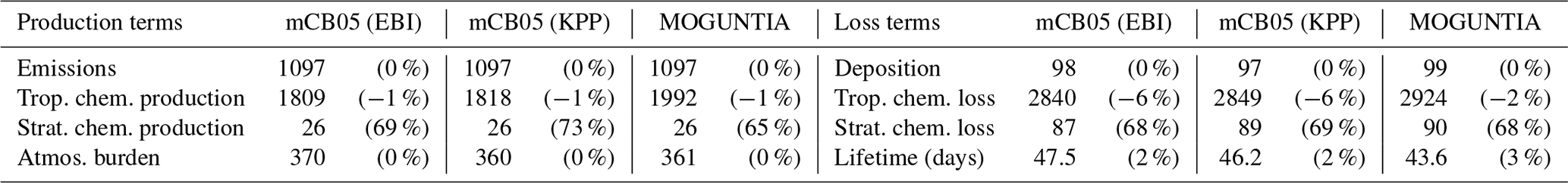
Figure 1 Simulated annual mean surface (a, c, e) and zonal mean (b, d, f) O₃ mixing ratios (ppb) for the MOGUNTIA chemistry scheme for the year 2006 (a, b) and the respective differences compared to mCB05(KPP) (c, d); the surface and zonal mean absolute differences between mCB05(KPP) and mCB05(EBI) are also presented (e, f).

Ozone surface and zonal mean mixing ratios simulated by the MOGUNTIA configuration for the year 2006 are presented in Fig. 1a and b, respectively. Figure 1c and d show small differences in surface and zonal mean mixing ratios between MOGUNTIA and mCB05(KPP). Differences in surface simulated O₃ mixing ratios between the two mechanisms are evident mainly downwind of regions with biogenic and tropical fire emissions. The mCB05(KPP) simulation shows higher mixing ratios (∼ 2–4 ppb) over the Intertropical Convergence Zone (ITCZ), India, and East Asia (up to ∼ 10 ppb). This is mainly attributed to the different representation of VOCs, with MOGUNTIA being significantly more explicit than mCB05. This behavior can also be observed in the zonal mean O₃ distribution presented in Fig. 1d, where the impact of the different representation of VOCs, originating mainly from the tropics, is reaching the middle and upper troposphere lifted by convection following the upward branch of the tropical Hadley cell. The use of different solvers alone does not result in any critical difference in the O₃ mixing ratios for mCB05 (Fig. 1e, f), presenting only some small negative differences of ∼ 1 ppb downwind of regions with high anthropogenic emissions (e.g., India) for mCB05(EBI).

4.2 Hydroxyl radical (OH)

The hydroxyl radical (OH) is the primary oxidant in the atmosphere under sunlit conditions, initiating the oxidation of various VOCs and thus the production of hydroperoxy (HO₂) and organic peroxy (RO₂) radicals. However, due to the high complexity of OH recycling pathways in atmospheric VOC degradation, the different representations of VOC oxidation pathways in chemical mechanisms may lead to significant discrepancies between models. CH₄ is routinely used as a diagnostic for the calculated OH abundance in the troposphere since its background concentration is highly sensitive to the OH abundance in the tropics, where water vapor and biogenic emissions are high. Uncertainties in CH₄ global sources (e.g., a rapid rise in the CH₄ growth rates since 2007; Nisbet et al., 2019), together with uncertainties in anthropogenic emissions of NO_x, CO, and NMVOCs (e.g., Hoesly et al., 2018), may cause considerable divergence in model-simulated CH₄ mixing ratios for different simulation years. For the present study, however, the surface mixing ratios of CH₄ are prescribed according to the CMIP6 recommendations for each simulation year.

Table 5 Tropospheric chemical budget of OH for the year 2006 (Tg(OH) yr⁻¹) using the 150 ppb O₃ mixing ratio to define the tropopause level. In parentheses, the relative differences using the 100 ppb O₃ mixing ratios are also presented, calculated with reference to the 150 ppb O₃ tropopause level definition.

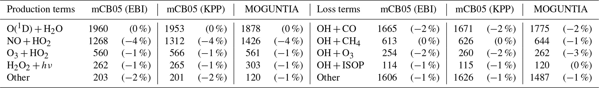
Table 5 presents the global tropospheric OH production budgets for the various chemical configurations. The MOGUNTIA configuration yields a gas-phase OH formation via O₃ photolysis in the presence of water molecules (Reactions R3 and R4) of about 1878 Tg yr⁻¹. Additionally, the radical recycling terms (Reactions R1 and R5) contribute 1987 Tg yr⁻¹, the H₂O₂ photodissociation, i.e.,

$$\begin{array}{}\text{(R7)}& {\mathrm{H}}_{\mathrm{2}}{\mathrm{O}}_{\mathrm{2}}+h\mathit{\nu }\to \mathrm{2}\mathrm{OH},\end{array}$$

produces 303 Tg yr⁻¹, and all other reactions add another 120 Tg yr⁻¹ to the global tropospheric OH production in the model. Overall, the total tropospheric OH production amounts to 4288 Tg yr⁻¹, which is in close agreement with the budget estimations by Lelieveld et al. (2016), i.e., ∼ 4270 Tg yr⁻¹. Some difference is, however, expected due to the definition of the troposphere in Lelieveld et al. (2016), who define the tropopause in the tropics using temperature and in the extratropics using potential vorticity gradients. We remind the reader that for the present study the chemical troposphere is defined using a threshold of 150 ppb O₃. It is striking that the OH chemical production calculated for the MOGUNTIA model setup is much higher (28 %–35 %) than for previous TM5 model configurations (i.e., 3355±30 and 3184±20 Tg yr⁻¹) as presented by van Noije et al. (2014) using a similar 150 ppb O₃ tropopause. This difference is mainly attributed to the various updates of the model compared to the version used in Noije et al. (2014), such as the emission database and the applied VOC representation (i.e., CMIP5; Lamarque et al., 2010, vs. CMIP6 for this study), the chemistry scheme (i.e., CB4 vs. MOGUNTIA), and the photolysis scheme (i.e., the previous implemented Landgraf et al., 1998, photolysis scheme vs. the modified band approach scheme implemented by Williams et al., 2012).

Focusing on the differences between the MOGUNTIA and mCB05(KPP) mechanism, the MOGUNTIA OH production is very close to mCB05(KPP) on a global scale (Table 5). Note that for mCB05, the comparison of the two solvers indicates that EBI calculates a ∼ 1 % lower chemical destruction of OH in the troposphere than Rosenbrock. The contributions of the CO and CH₄ oxidation terms to the global tropospheric OH losses are calculated as 41 % and 15 %, respectively, for the MOGUNTIA scheme. This is slightly higher (by ∼ 6 % and ∼ 3 %, respectively) compared to mCB05(KPP).

Focusing further on the MOGUNTIA scheme, the calculated tropospheric CH₄ chemical lifetime is ∼ 8.0 years, as obtained by dividing the CH₄ global atmospheric mean burden (∼ 4871 Tg) by the loss due to oxidation by OH radicals in the troposphere (∼ 607 Tg yr⁻¹). Accounting, however, for additional CH₄ sinks due to oxidation in soils and the stratosphere with assumed lifetimes of 160 and 120 years (Ehhalt et al., 2001), respectively, an atmospheric lifetime of about 7.18 years is derived, which is roughly 15 % shorter than the ensemble model mean atmospheric lifetime reported by Stevenson et al. (2006) of 8.45±0.38 years. The multi-model chemistry–climate simulations performed during the Atmospheric Chemistry and Climate Model Intercomparison Project (ACCMIP) (Naik et al., 2013; Voulgarakis et al., 2013) revealed vast diversities among models, with a wide range of CH₄ chemical lifetime values (i.e., ∼ 7–14 years) and a mean value of 9.7±1.5 years (i.e., 5 %–10 % higher than observation-derived estimates). Lelieveld et al. (2016) derived a CH₄ chemical lifetime of 8.5 years for the year 2010, and Schultz et al. (2018) estimated a tropospheric CH₄ chemical lifetime of about 9.9 years also using an O₃ threshold of 150 ppb to define the tropopause. Finally, Lamarque et al. (2012) reported a chemical lifetime of ∼ 8.7 years by taking a tropopause level at 100 ppb O₃.

Table 6 Global budgets and burden (Tg(CO)) of CO for the year 2006 (Tg(CO) yr⁻¹) using the 150 ppb O₃ mixing ratio to define the tropopause level. In parentheses, the relative differences using the 100 ppb O₃ mixing ratios are also presented, calculated with reference to the 150 ppb O₃ tropopause level definition.

4.3 Carbon monoxide (CO)

Table 6 presents the chemical CO budget calculated by TM5-MP for the three chemical configurations. The different model configurations show that approximately 62±1 % of the CO global production in the troposphere is due to the oxidation of CH₄ and NMVOCs, with the remaining due to direct emissions. Overall, the global CO budget is significantly affected by the interactions between OH and CO. Thus, changes in OH tropospheric chemical production (i.e., ∼ −0.2 % from mCB05(KPP) to MOGUNTIA) modulate the tropospheric secondary formation of CO from the oxidation of CH₄ and NMVOCs (∼ −10 % change) as well as the CO chemical loss (∼ −3 % change) in the model. The global chemical production (i.e., the sum of chemical production terms in the troposphere and stratosphere; Table 6) of CO for both the MOGUNTIA and mCB05(KPP) chemical configurations, i.e., 2018 and 1844 Tg yr⁻¹, respectively, is, however, higher than the multi-model mean estimate (1505±236 Tg yr⁻¹) reported by Shindell et al. (2006), which can be partially attributed to the different year of NMVOC emissions used (i.e., 2000 vs. 2006 for this work).

The dominant chemical reaction responsible for the increase in tropospheric CO chemical production for MOGUNTIA compared to the mCB05(KPP) chemical configuration is the HCHO oxidation by OH radicals (i.e., ∼ 15 % increase compared to mCB05(KPP)). Indeed, although the lumped nature of the mCB05(KPP) mechanism leads to a higher tropospheric HCHO chemical production (∼ 1896 Tg yr⁻¹) compared to the MOGUNTIA configuration (∼ 1843 Tg yr⁻¹), the HCHO tropospheric chemical destruction is calculated roughly 2 % higher for the MOGUNTIA scheme. HCHO is mainly formed via the oxidation of CH₄, isoprene, and other NMVOCs in the model. However, for both mCB05 configurations, the HCHO production via CH₃O₂H photolysis is calculated to be ∼ 1.65 times higher compared to MOGUNTIA. The latter scheme seems to recycle the methyl-peroxy radical (CH₃O₂) more efficiently via CH₃O₂ gas-phase reactions with organic peroxy radicals (RO₂) produced by higher-order NMVOC oxidation. In contrast, other higher aldehydes that represent the second-most important producer of CO contribute more significantly in MOGUNTIA than in mCB05. This could be due to the more detailed representation of the higher aldehydes in the MOGUNTIA mechanism (e.g., considering the production and destruction reaction of GLY, GLYAL, and C₂H₅CHO) compared to the single lumped species (i.e., the ALD2) that represents all higher aldehydes in mCB05.

The global annual mean burden of CO for the MOGUNTIA chemical scheme is 361 Tg, almost the same as in the mCB05(KPP) configuration but ∼ 2 % lower compared to mCB05(EBI). Higher CO losses by OH oxidation and deposition in MOGUNTIA lead to a CO atmospheric lifetime of ∼ 44 d, i.e., about 6 % shorter compared to the mCB05(KPP) chemical mechanism. Note that the reduction in the atmospheric lifetime of CO is in line with the reduction in the atmospheric lifetime of CH₄ (∼ 3 %), reflecting an overall increase in tropospheric OH mixing ratios for the MOGUNTIA configuration compared to mCB05(KPP); i.e., higher OH levels in the atmosphere lead to proportionally larger CO and CH₄ sinks.

Focusing further on the impact of the solver alone, we calculate roughly a 3 % reduction in the CO atmospheric burden when the EBI solver is applied to the mCB05 mechanism in the model. This is directly connected to the ∼ 1 % increase in OH mixing ratios that is calculated when the Rosenbrock solver is used in the model. Furthermore, the CO tropospheric production is increased by ∼ 0.5 % in mCB05(KPP) compared to mCB05(EBI). Overall, the presented differences between the EBI and Rosenbrock solvers confirm that the choice of solver may impact the simulated mixing ratios, owing mainly to the use of a constant versus a variable time step in the chemistry integration (see, e.g., Sandu et al., 1997).

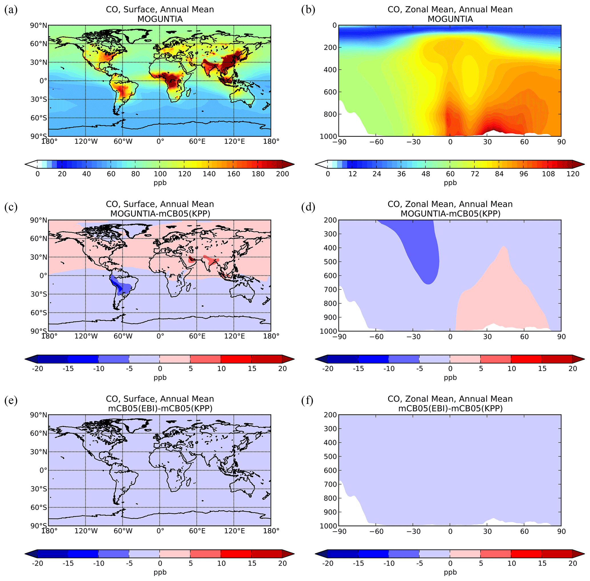
Figure 2 Simulated annual mean surface (a, c, e) and zonal mean (b, d, f) CO mixing ratios (ppb) for the MOGUNTIA chemistry scheme for the year 2006 (a, b) and the respective differences compared to mCB05(KPP) (c, d); the surface and zonal mean absolute differences between mCB05(KPP) and mCB05(EBI) are also presented (e, f).

Zonal mean CO mixing ratios at the surface for the year 2006 using the MOGUNTIA scheme are presented in Fig. 2a and b. Compared to mCB05(KPP), the results from MOGUNTIA show slightly higher surface CO mixing ratios (up to ∼ 2 ppb) over highly populated regions, such as India. This regional increase is due to the differences in surface OH mixing ratios, owing mainly to the differences in NO_x chemistry between the two simulations (see also Sect. 5.2). In contrast, in South America negative differences of ∼ 5–15 ppb are calculated at the surface (Fig. 2c). The effective HO_x regeneration together with the detailed VOC representation and oxidation pathways considered in MOGUNTIA result in an increase in the surface OH mixing ratios in locations with high biogenic VOC emissions. This subsequently leads to a regional decrease in the tropospheric CO mixing ratios compared to the mCB05(KPP) configuration. Similar results are found for the zonal mean CO distribution. Free tropospheric CO mixing ratios in the tropics are also affected due to effective tropical convection. Finally, the use of different solvers for the mCB05 mechanism does not lead to any notable differences in the annual mean CO mixing ratios (Fig. 2e, f).

5 Model evaluation

Model simulations are evaluated with a series of surface, flask, aircraft, and sonde measurements, as well as with satellite retrievals and climatological data. The simulated NO₂ tropospheric columns are compared with satellite retrievals from the European Quality Assurance for Essential Climate Variables (QA4ECV) project (Boersma et al., 2017), provided by the Ozone Monitoring Instrument (OMI) and the SCanning Imaging Absorption SpectroMeter for Atmospheric CHartographY (SCIAMACHY). The simulated OH mixing ratios are evaluated against calculations of global mean tropospheric values from other modeling studies and against climatological data compiled by Spivakovsky et al. (2000). Modeled O₃ mixing ratios are evaluated against surface observations and ozonesonde data for the year 2006, as compiled by the World Ozone and Ultraviolet Radiation Data Centre (WOUDC; http://www.woudc.org; last access: 20 August 2019); surface observations from the European Monitoring Evaluation Program network (EMEP; http://www.emep.int; last access: 20 August 2019) have been also used. For the CO model evaluation, flask observations for the year 2006 are used, as compiled by the National Oceanic and Atmospheric Administration Earth System Research Laboratory, Global Monitoring Division (NOAA; https://www.esrl.noaa.gov/gmd; last access: 20 August 2019). O₃ and CO mixing ratios in the upper troposphere–lower stratosphere (UTLS) are compared to in situ measurements from the MOZAIC (Measurement of Ozone and Water Vapour by Airbus In-Service Aircraft) data record (Thouret et al., 1998). The modeled CO total columns are compared with satellite retrievals from the Measurement of Pollution in the Troposphere (MOPITT) instrument version MOP02J_V008 (Deeter et al., 2013, 2019; Ziskin, 2019), i.e., the combined thermal–near-infrared data product. Finally, light VOCs (i.e., C₂H₄, C₂H₆, C₃H₆, C₃H₈) as simulated for the year 2006 are evaluated against flask measurements from the NOAA database and against climatological data from aircraft campaigns, as produced by Emmons et al. (2000). Overall, to quantify and discuss the model performance, commonly used statistical parameters are calculated, such as the correlation coefficient (R), which reflects the strength of the linear relationship between model results and observations (the ability of the model to simulate the observed variability), the absolute bias (BIAS), the normalized mean bias (NMB), and the root mean square error (RMSE) as a measure of the mean deviation of the model from the measurement due to random and systematic errors. All equations used for the statistical analysis of model results are provided in the Supplement (Eqs. S1–S5).

Figure 3 Annual mean comparison of tropospheric NO₂ vertical columns (molec. cm⁻²) for the two chemistry schemes MOGUNTIA and mCB05(KPP) (a, b) against the Ozone Monitoring Instrument (OMI) satellite data (c, d) using the respective averaging kernel information for 2006. The absolute (e, f) and relative (g, h) differences are also presented.

5.1 Nitrogen dioxide (NO₂)

NO_x is a rate-limiting precursor of O₃ formation and thus an essential species for other tropospheric oxidants, such as OH. NO_x is emitted by both natural (lightning, soils, and fires) and anthropogenic combustion sources, with lightning mainly impacting NO_x mixing ratios at the top of convective updrafts and anthropogenic fuel emissions being the principal source of NO at the surface. Tropospheric NO₂ vertical column densities retrieved from OMI (Boersma et al., 2017) are compared against the MOGUNTIA and mCB05(KPP) simulations (Fig. 3). Note that since the differences between mCB05(EBI) and mCB05(KPP) are small for tropospheric NO₂ columns, mCB05(EBI) is not shown. NO₂ column densities are retrieved using a consistent set of retrieval parameters and validated against ground-based MAX-DOAS measurements (Boersma et al., 2018). To consider the vertical sensitivity of the satellite measurements to NO₂ molecules at different altitudes, the tropospheric column averaging kernels provided in the QA4ECV data product are applied separately to both sets of modeled NO₂ vertical profiles, extracted from the hourly 3-D model output by linear and nearest-neighbor interpolation in space and time. The resulting NO₂ tropospheric column density is what would have been retrieved by the satellite if the actual vertical profile of NO₂ mixing ratios were identical to the modeled profile. The tropospheric NO₂ columns retrieved from the satellite are averaged per model grid cell and day, resulting in a comparison dataset consisting of one NO₂ vertical column density per model grid cell and day.

For the MOGUNTIA configuration, the model shows a mean overestimation of 1.78×10¹⁴ (R=0.71) and 1.96×10¹⁴ molec. cm⁻² (R=0.95) against OMI measurements for daily and annual values, respectively, performing slightly better than the correlation of the mCB05(KPP) configuration (R=0.71 and R=0.94 for daily and annual values). An overview of the statistical comparison of the three model simulations against OMI measurements is given in Fig. S1a. Some discrepancies, especially in the Northern Hemisphere (NH), may be attributed to the absence of a significant seasonal cycle in monthly anthropogenic emissions. Over the biomass burning source regions in Africa, the model overestimates the satellite retrievals. When the model is compared against NO₂ tropospheric columns from the SCIAMACHY instrument using the QA4ECV retrieval (not shown), the MOGUNTIA configuration shows a similar improvement over mCB05(KPP), as with the OMI data.

Williams et al. (2017) showed that the TM5-MP model significantly underestimates the NO and NO₂ mixing ratios, both at the surface and in vertical profiles. The model satisfactorily reproduces the NO₂ mixing ratios in the boundary layer but overestimates mixing ratios at higher altitudes and in pristine environments. The MOGUNTIA scheme shows generally better agreement with satellite retrievals compared to the mCB05(KPP) configuration, as expressed by a higher correlation coefficient and a generally lower bias (Fig. S1a). The differences between the two chemistry schemes can be mainly attributed to the representation of organic NO_x reservoir species (i.e., the organic nitrates; ORGNTRs) in the two mechanisms (Fig. S2). Overall, since deep convection may efficiently transport ORGNTRs to the upper troposphere, the more explicit representation of VOC chemistry in the MOGUNTIA chemistry scheme alters the distribution of ORGNTRs compared to the more lumped chemistry of mCB05. Although production of ORGNTRs is about 10 % larger in the MOGUNTIA scheme, the ORGNTR burden is dominated by the loss term (Table S4). Due to the more detailed ORGNTR representation in the MOGUNTIA scheme, the destruction becomes significantly more efficient compared to the mCB05 configuration. As a result, the global ORGNTR burden calculated using the MOGUNTIA scheme in the model is about 60 % smaller.

Several modeling studies have compared simulated NO₂ columns with in situ and satellite observations (e.g., Travis et al., 2016; Williams et al., 2017). These studies demonstrated an overestimate of the observed $\mathrm{NO}/{\mathrm{NO}}_{\mathrm{2}}$ ratios compared to observations at higher altitudes, possibly due to a respective underestimate of peroxy radicals in the upper troposphere that contributes to the NO to NO₂ conversion. A deviation in the $\mathrm{NO}/{\mathrm{NO}}_{\mathrm{2}}$ ratio has also been reported for the GEOS-Chem model (Silvern et al., 2018; Travis et al., 2016). This model significantly underestimated the observed upper tropospheric NO₂ observations from the SEAC⁴RS aircraft campaign over the southeast United States. Silvern et al. (2018) calculated the reaction with ozone to account for roughly 75 % of the NO to NO₂ conversion in the upper troposphere; thus, this deviation from the photochemical equilibrium could be due to an error in kinetic data. Overall, the authors indicated that reducing the NO₂ photolysis by 20 % and increasing the low-temperature NO+O₃ reaction rate constant by 40 % improves the model simulation of the $\mathrm{NO}/{\mathrm{NO}}_{\mathrm{2}}$ ratio in the upper tropospheric data significantly compared to the aircraft data. Another source of uncertainty could be the strength of the direct soil emissions that, according to Miyazaki et al. (2017), are lower in our model (i.e., ∼ 5 Tg N yr⁻¹; Yienger and Levy, 1995) compared to the emissions of 7.9 Tg N yr⁻¹ derived using a multi-constituent satellite data assimilation.

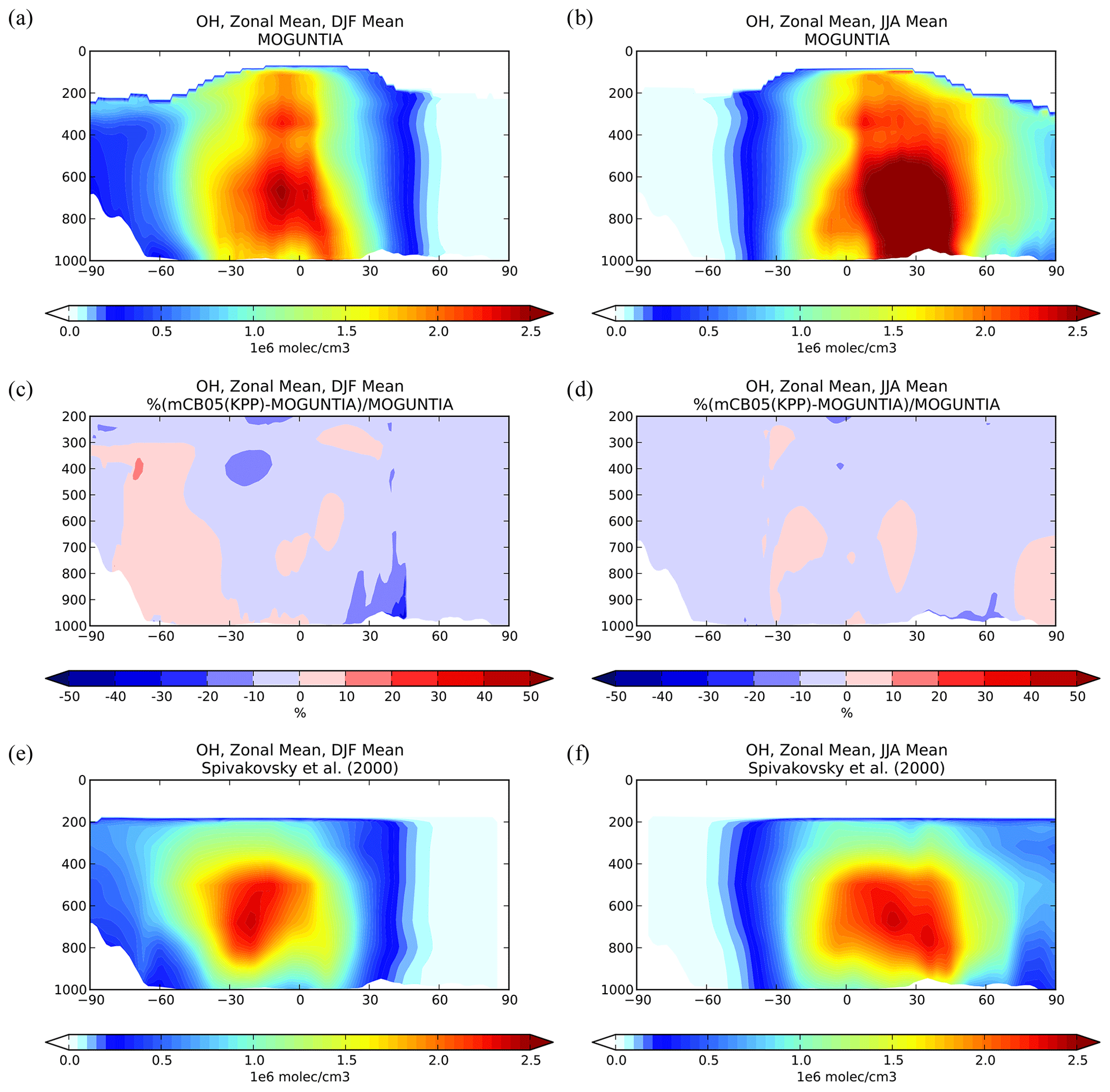
Figure 4 Zonal mean OH mixing ratios for December–January–February (DJF; a, c, e) and June–July–August (JJA; b, d, f) 2006, as simulated by the TM5-MP model with the MOGUNTIA chemistry scheme (a, b). The differences (%) between the mCB05(KPP) and the MOGUNTIA chemical configuration (c, d) and the optimized climatological average from Spivakovsky et al. (2000) up to 200 hPa (e, f).

5.2 Hydroxyl radical (OH)

Figure 4a and b illustrate the zonal mean tropospheric distributions of OH for two seasons (i.e., boreal winter and boreal summer) for 2006, as simulated with the MOGUNTIA chemistry scheme. The highest atmospheric mixing ratios of OH in the model are calculated in the tropics from close to the surface up to roughly the tropopause as a result of intense solar radiation and high humidity in the region, with the main OH maximum being roughly below 400 hPa (and a secondary maximum at ∼ 300 hPa). The differences in OH zonal mean mixing ratios compared to the mCB05(KPP) configuration are presented in Fig. 4c and d. During the boreal winter, the mCB05(KPP) configuration results on average in lower OH mixing ratios in the northern subtropical lower troposphere (∼ 3 %–6 %) than the MOGUNTIA simulation (Fig. 4c), with the largest differences (∼ 20 %–30 %) around 20–40^∘ N. In the subtropical Southern Hemisphere (SH) during boreal summer, OH mixing ratios are on average lower (∼ 2 %–3 %) in the MOGUNTIA configuration than in mCB05(KPP) (Fig. 4d) almost everywhere, except for a small increase (up to 10 %) at around 30^∘ S. These small differences in OH mixing ratios are mainly related to the HO_x regeneration and differences in NO_x and ORGNTR species that influence the distribution of OH in the troposphere. The more detailed representation of ORGNTRs in the MOGUNTIA chemistry scheme results in more efficient NO_x release upon ORGNTR destruction (Table S4), leading overall to O₃ formation in remote locations and thus to the stimulation of HO_x recycling at higher altitudes. Note that globally the NO+HO₂ reaction is roughly 9 % higher in the MOGUNTIA configuration on an annual basis compared to mCB05(KPP) (see Table 5).

Focusing on global means, a global mean tropospheric OH concentration of 10.1×10⁵ molec. cm⁻³ is obtained from the MOGUNTIA chemistry configuration for the year 2006, which is roughly 4 % higher than in the mCB05(KPP) configuration but closer to the low end of the multi-model mean of $\mathrm{11}\pm \mathrm{1.6}\times {\mathrm{10}}^{\mathrm{5}}$ molec. cm⁻³ as derived by Naik et al. (2013) for the year 2000 and the mean tropospheric mixing ratios of 11.3×10⁵ molec. cm⁻³ as calculated by Lelieveld et al. (2016) for the year 2013. In the tropical troposphere (30^∘ S–30^∘ N), the mean OH level in the MOGUNTIA configuration of 16.74×10⁵ molec. cm⁻³ is ∼ 6 % higher than in mCB05(KPP). In all model configurations, higher OH mixing ratios are calculated in the NH compared to the SH, which is directly related to the asymmetry in the hemispheric O₃ and NO_x burdens. Figure 4e and f show the climatological mean OH mixing ratios from the surface up to ∼ 200 hPa from Spivakovsky et al. (2000), reduced by 8 % based on the observed decay of methyl-chloroform mixing ratios (see Huijnen et al., 2010; van Noije et al., 2014). The mean tropospheric OH concentration for the MOGUNTIA configuration is calculated to be roughly 25 % and 30 % higher compared to the optimized climatology from Spivakovsky et al. (2000) for boreal winter and summer, respectively. Moreover, a ∼ 28 % higher NH $/$ SH ratio of annual mean hemispheric OH mixing ratios in the troposphere is derived for the MOGUNTIA configuration compared to Spivakovsky et al. (2000). The NH $/$ SH ratios are calculated as ∼ 1.37 and ∼ 1.35 for the MOGUNTIA and mCB05(KPP) configuration, respectively, being on the high end of other modeling estimates, such as the multi-model estimate of an NH $/$ SH ratio of 1.28±0.10 by Naik et al. (2013) and the 1.20 ratio reported by Lelieveld et al. (2016).

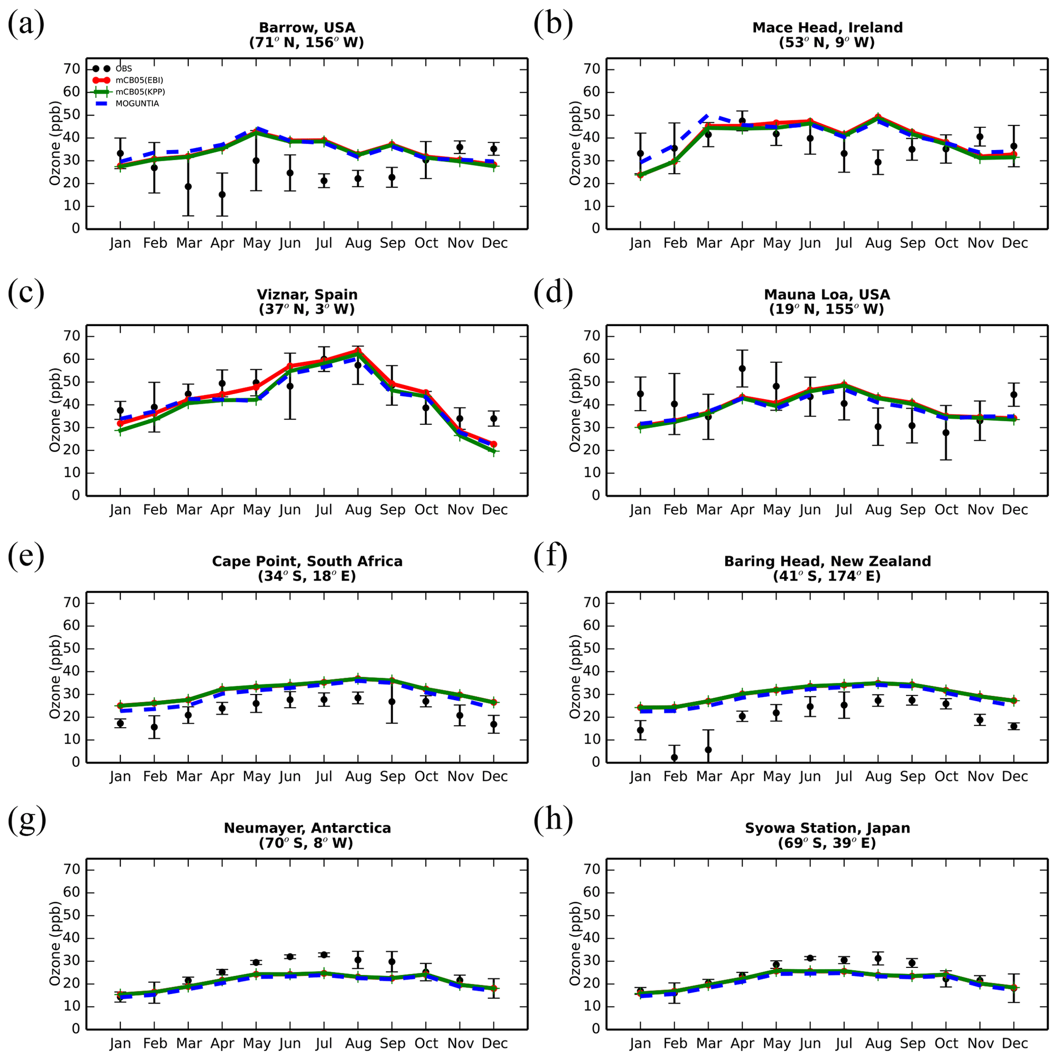
Figure 5 Monthly mean comparison of TM5-MP surface O₃ (ppb) against surface observations (black line) from EMEP and WOUDC databases for the two chemistry schemes, mCB05(KPP) (green line) and MOGUNTIA (blue line), using colocated model output for 2006 sampled at the measurement times; error bars indicate the standard deviation in the monthly means. For comparison, model results of mCB05 with the EBI solver (red line) are also presented.

5.3 Ozone (O₃)

The evaluation of modeled O₃ mixing ratios against surface observations for the three simulations for the year 2006 is presented in Fig. 5. The seasonal cycle across surface stations is generally well captured by all model configurations for most of the cases. TM5-MP, however, generally overestimates O₃ mixing ratios at most NH sites and for all model configurations, as can be seen, for example, at the Barrow (Fig. 5a) and Mace Head (Fig. 5b) stations, especially during the summer (June–July–August, JJA) season when O₃ is overestimated by about 8 and 3 ppb, respectively. However, at Víznar (Spain) and Mauna Loa (USA) (Fig. 5c and d, respectively), model results are closer to the observed O₃ mixing ratios, showing overall lower biases (i.e., ∼ 1–3 ppb). In the SH (except for the polar circle), the model simulates the seasonal cycle of the O₃ surface mixing ratios well but with average positive biases of ∼ 6–10 ppb in Cape Point (South Africa) and Baring Head (New Zealand) (Fig. 5e, f). At the South Pole (USA) and Syowa (Japan) stations in Antarctica (Figs. 5g, h), the model also captures the observed seasonality well ($R=\sim$ 0.9), except for a negative bias of ∼ 3 ppb during the local winter season. Focusing further on the chemistry mechanisms applied in the model, slightly better consistency is achieved for the MOGUNTIA chemistry scheme in most of the cases. For the mCB05 chemistry scheme, the choice of the solver does not result in any notable difference in simulated surface O₃ mixing ratios. Considering all surface O₃ observations available for the year 2006 (Fig. S3), the MOGUNTIA chemistry configuration tends to overestimate the available observations with a mean bias of ∼ 6.5 ppb. Note that although the differences between the chemistry configurations for surface O₃ are small, the mCB05(KPP) configuration shows the lowest bias (∼ 5.2 ppb), whereas the mCB05(EBI) bias is closer to that of the MOGUNTIA configuration (∼ 6.1 ppb).

Figure 6 Monthly mean comparison of TM5-MP O₃ (ppb) against sonde observations (black dots; mean and standard deviation) at (a) Hohenpeissenberg and (b) Macquarie Island for different pressure levels (900, 800, 500, 400, 200 hPa) for the two chemistry schemes, mCB05(KPP) (green line) and MOGUNTIA (blue line), using colocated model output for 2006 sampled at the measurement times; error bars indicate the standard deviation in the monthly means. For comparison, the results of mCB05 with the EBI solver (red line) are also presented.

Ozonesonde observations are used to evaluate the models' ability to reproduce the O₃ vertical profiles. Indicatively, Fig. 6 presents the comparison of model results with ozonesonde observations in 2006 at Hohenpeissenberg in Germany and at Macquarie Island in the southwestern Pacific Ocean at five pressure levels (900, 800, 500, 400, and 200 hPa) covering the boundary layer and the low and high free troposphere. For this evaluation, all ozonesonde data have been binned to the 34 model pressure levels (see Sect. 2.5). The seasonal cycle at the two stations is well captured by each model configuration. For the highest model levels above 200 hPa, all simulations are very close to the measurements, since O₃ mixing ratios are mainly determined by the upper boundary condition that is used (see Sect. 2.1). Comparisons for other WOUDC stations around the globe for the year 2006 are presented in the Supplement (Fig. S4). Overall, all model simulations capture the O₃ distribution quite well at almost all sites in the lower troposphere. The MOGUNTIA scheme shows slightly better agreement with observations than the mCB05 configurations, with smaller biases in most of the cases, especially at lower levels (i.e., from ∼ 900 hPa and up to ∼ 500 hPa). Concerning the impact of the chemistry solver, the vertical O₃ concentration simulated using the mCB05 mechanism shows no notable differences between the use of KPP and EBI in most of the cases. Overall, considering all available ozonesonde data for the year 2006 (Fig. S4), the MOGUNTIA chemistry in TM5-MP results in an overestimation of the ozonesonde observations by roughly 16 % (R=0.96, BIAS = 4.7 ppb, NME = 15.6 %), which is slightly smaller compared to the mCB05 chemistry configurations.

Figure S5 presents a comparison of O₃ mixing ratios in the upper troposphere–lower stratosphere (UTLS) simulated by TM5-MP for the two chemistry configurations (i.e., mCB05(KPP) and MOGUNTIA), with in situ observations from the MOZAIC airborne program (see Sect. 3.1), as a function of latitude. The accuracy of the MOZAIC O₃ measurements is ±2 ppb (Marenco et al., 1998). For this comparison, the MOZAIC measurements are binned on the vertical grid of TM5-MP. The model evaluation at pressure levels < 300 hPa indicates there is good agreement of both configurations with the observed mixing ratios. A positive bias in April of the order of ∼ 20 ppb is calculated for the model, but smaller biases are found around the tropics and at latitudes north of 40^∘ N (Fig. S5a). In October (Fig. S5b), a constant positive bias of roughly 20 ppb is calculated for both configurations. This could be caused by the limited vertical resolution of this model version in the UTLS region. Note that 34 vertical levels were employed for this study with a higher resolution in the upper troposphere–lower stratosphere region. Part of the model overestimation could also be attributed to systematic errors, as also reported in previous studies (e.g., Huijnen et al., 2010). Possible causes include cumulative effects such as a lack of diurnal or weekly variation in the NO_x emissions from the road transport sector, an underestimation of surface deposition during summer, or errors in the representation of nocturnal boundary layer dynamics (see, e.g., Williams et al., 2012).

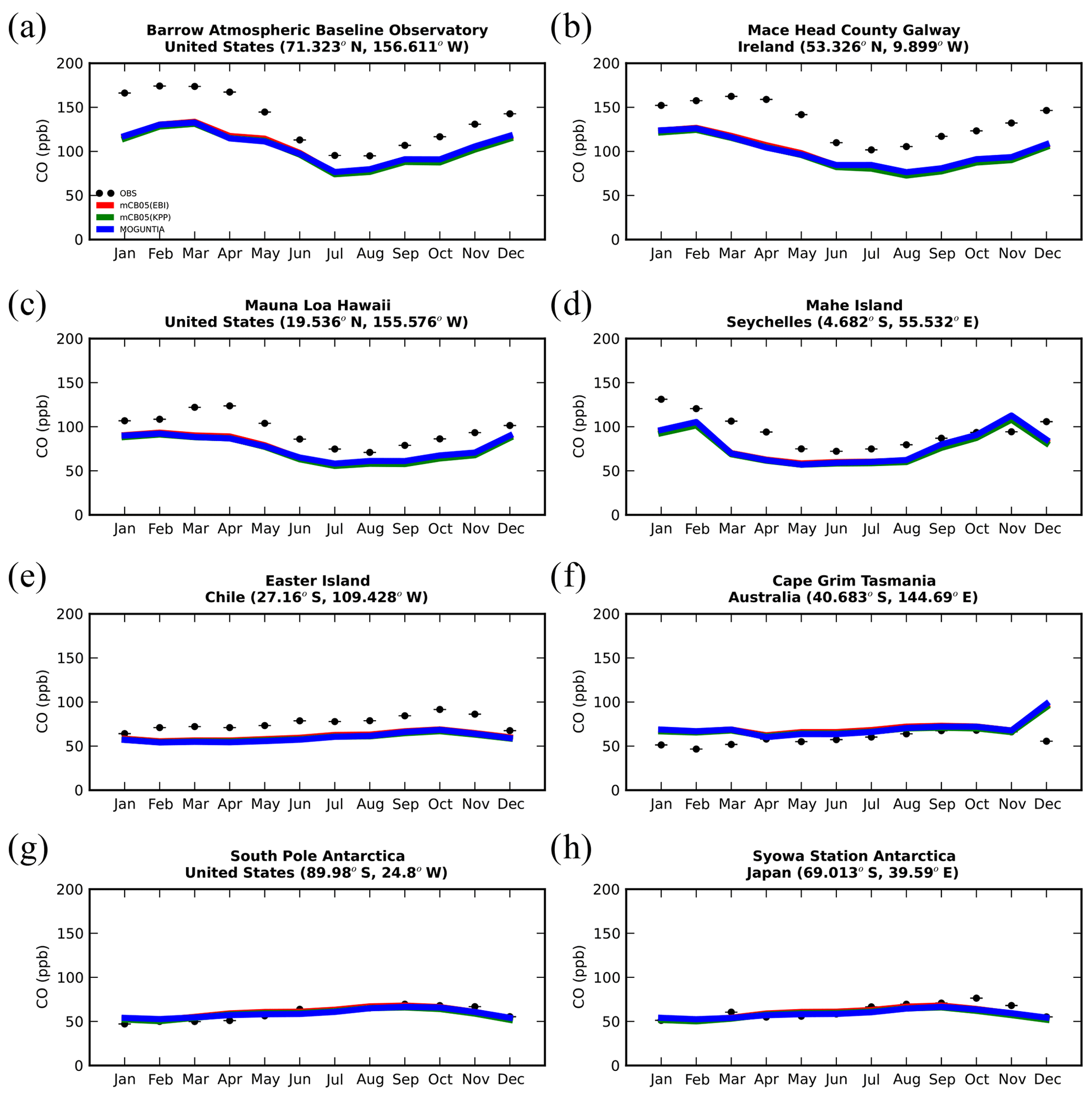
Figure 7 Monthly mean comparison of TM5-MP surface CO (ppb) against flask measurements (black line) for the two chemistry schemes, mCB05(KPP) (green line) and MOGUNTIA (blue line), using colocated model output for 2006 sampled at the measurement times; error bars indicate the standard deviation in the monthly means. For comparison, model results of mCB05 with the EBI solver (red line) are also presented.

5.4 Carbon monoxide (CO)

Figure 7 presents the model performance concerning surface CO mixing ratios by comparing a series of flask observations for the year 2006. CO is underestimated at most sites in the NH for all TM5-MP configurations, e.g., at the Barrow Observatory and Mace Head station (Fig. 7a, b), especially during boreal spring (March–April–May, MAM), by about 30 ppb on average. In the tropics, negative biases (∼ 16–20 ppb) are observed at Mauna Loa and Mahé island (Fig. 7c, d). At other stations in the SH, the model simulates the CO surface mixing ratios well, with both positive and negative biases depending on the season (Fig. 7e, f). In Antarctica, at the South Pole and Syowa stations (Fig. 7g, h), the model also shows a small positive bias up to ∼ 3 ppb during the local winter season. The seasonal cycle across stations is generally well captured by all model chemistry configurations (i.e., R= 0.7–0.9). The full set of CO comparisons with flask data is further presented in the Supplement (Fig. S6). Overall, the MOGUNTIA and mCB05(KPP) configurations underestimate the flask observations for the year 2006, with a negative bias of around 30 ppb and a correlation coefficient for both configurations of R=0.45. Notably, the mCB05(EBI) model configuration tends to produce lower biases in the SH, where emission strengths are in general low, compared to the other two configurations (i.e., approximately −3 vs. −4 and -5 ppb for mCB05(KPP) and MOGUNTIA, respectively). In contrast, the MOGUNTIA chemistry configuration results in lower biases in the NH where the majority of anthropogenic emissions occur (i.e., approximately −30 vs. −31 and −33 ppb for mCB05(EBI) and mCB05(KPP), respectively).

Total CO columns from the MOGUNTIA and mCB05(KPP) model configurations are compared to the total column densities retrieved from the MOPITT satellite instrument (Deeter et al., 2013, 2019; Ziskin, 2019) for the year 2006 (Fig. 8). Co-sampling with averaging kernels has been applied to the modeled CO concentration profiles (i.e., in the same manner as for NO₂; see Sect. 5.1). Note that when the absolute difference in surface pressure between the MOPITT retrieval and the TM5-MP simulation is larger than 5 hPa, the measurements were excluded from the comparison. For the MOGUNTIA configuration, the model shows a mean underestimation of $-\mathrm{8.54}\times {\mathrm{10}}^{\mathrm{16}}$ (R=0.82) and $-\mathrm{1.18}\times {\mathrm{10}}^{\mathrm{17}}$ molec. cm⁻² (R=0.91) compared to daily and annual averages of MOPITT data, respectively. However, the correlation is slightly improved compared to the mCB05(KPP) configuration (R=0.78 and R=0.88 for daily and annual values, respectively). As in the comparison with surface data, the biases in total column CO in the MOGUNTIA and mCB05(KPP) configurations deteriorated compared to the mCB05(EBI) configuration, although biases are still small (∼ −5 % and ∼ −7 % for daily and annual values, respectively). As this pattern can be seen in both KPP configurations, this difference seems to be caused by the implementation of the more accurate Rosenbrock solver. An overview of the statistical comparison of the three model configurations against MOPITT CO measurements is given in Fig. S1b.

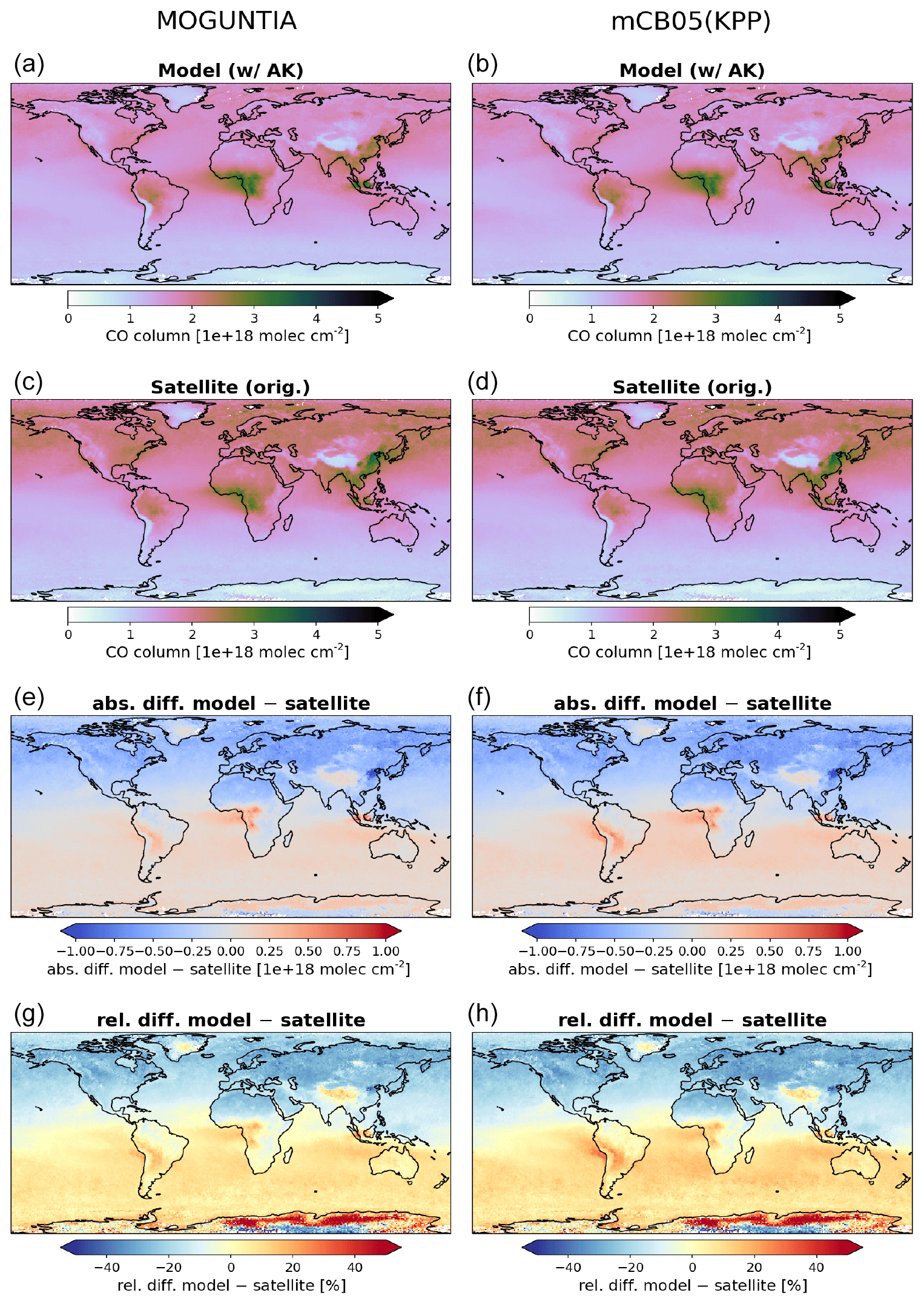
Figure 8 Annual mean comparison of total CO vertical columns (molec. cm⁻²) for the two chemistry schemes of TM5-MP, MOGUNTIA and mCB05(KPP) (a, b) against MOPITT satellite data (c, d), using the respective averaging kernel information for 2006. The absolute (e, f) and relative (g, h) differences are also presented.

Figure S5 further presents the comparison of CO mixing ratios in the upper troposphere–lower stratosphere (UTLS) simulated by TM5-MP with in situ measurements from the MOZAIC airborne program (see Sect. 3.1). Model evaluation at pressure levels < 300 hPa shows a good correlation for both configurations in the SH, with a small positive bias (up to ∼ 20 ppb) for the mCB05(KPP) configuration in April around the Equator and a small negative bias (∼ 10 ppb) for the MOGUNTIA configuration for latitudes below 10^∘ N. Both configurations present a strong negative bias (∼ 30 ppb) for latitudes above 20^∘ N (Fig. S5c). In October (Fig. S5d), both the mCB05(KPP) and MOGUNTIA configurations tend to underestimate the observations, with a negative bias of ∼ 20 ppb, except for a small positive bias between 0 and 20^∘ N. This positive model bias in the UTLS could point to a stronger convective uplift (e.g., Krol et al., 2018) in tropical Africa in April or to possible misrepresentations of biomass burning emission strengths and horizontal and vertical distributions (e.g., Daskalakis et al., 2015; Nechita-Banda et al., 2018). Indeed, MOZAIC data show an increase in CO mixing ratios from the NH (April) to the SH (October), mainly due to the impact of biomass burning processes. Overall, the model configurations in this work present both positive and negative biases compared to the MOZAIC observations, with observations indicating larger latitudinal CO variability than simulated.

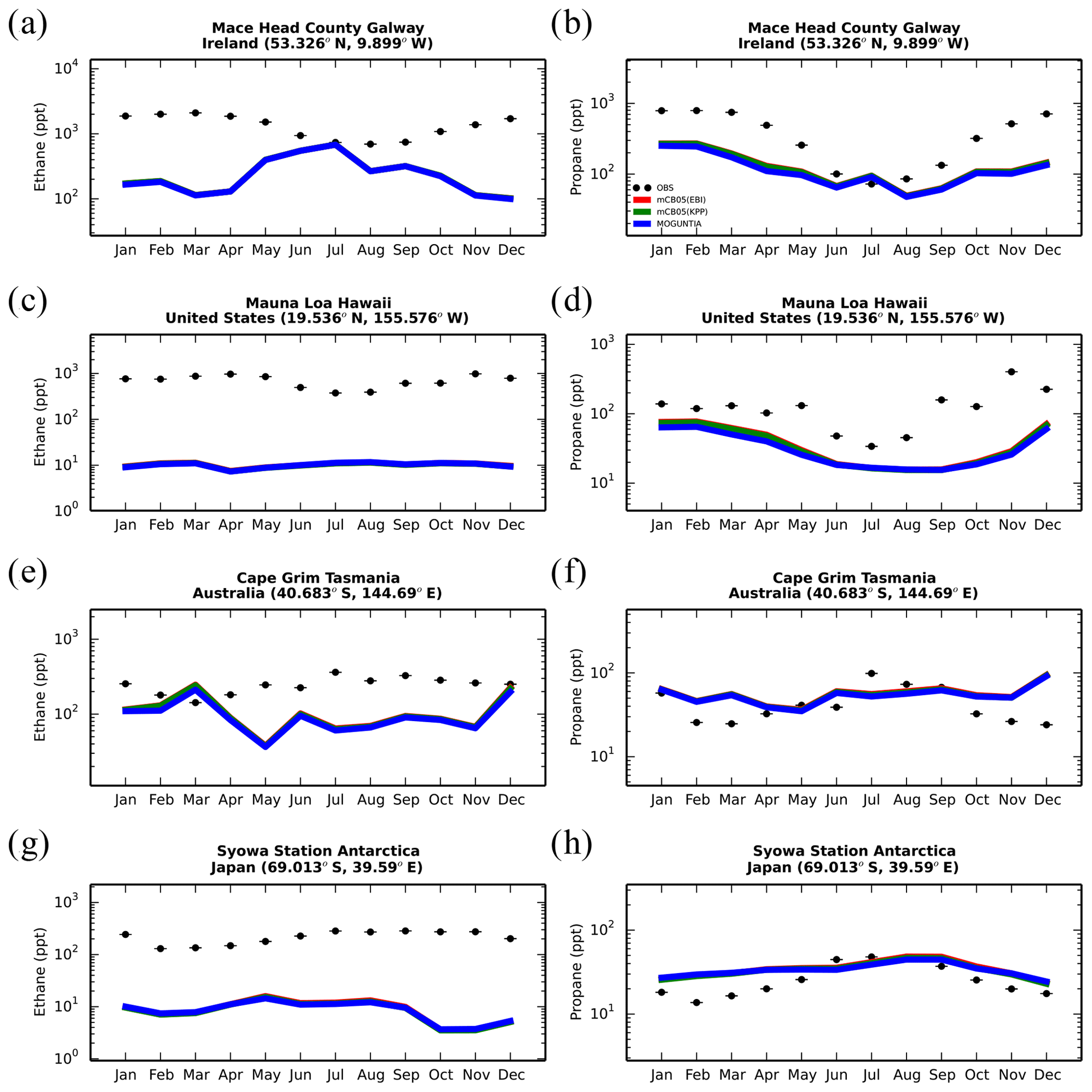
Figure 9 Monthly mean comparison of TM5-MP surface C₂H₆ (left column) and C₃H₈ (right column) against flask measurements (black dots; ppt) for the two chemistry schemes, mCB05(KPP) (green line) and MOGUNTIA (blue line), using colocated model output for 2006 sampled at the measurement times; error bars indicate the standard deviation in the monthly means. For comparison, model results of mCB05 with the EBI solver (red line) are also presented.

5.5 Volatile organic compounds (VOCs)

5.5.1 Ethane and propane

Ethane (C₂H₆) is the lightest alkane, with emissions primarily of anthropogenic origin associated mainly with fossil fuel extraction and use. In the model, the global ethane emission is 11 Tg yr⁻¹ (Table 3), with an atmospheric lifetime of about 56 d for all chemistry configurations, in close agreement with other studies (e.g., Hodnebrog et al., 2018). Flask measurements indicate that C₂H₆ surface mixing ratios are strongly underestimated by all configurations at Mace Head (Fig. 9a) by ∼ 80 %, mainly during the winter, also indicating an opposite annual cycle. The latter can be attributed to the misinterpretation of seasonal variation in anthropogenic emissions and/or to C₂H₆ oxidation by OH radicals in the model. Significant underestimations are also observed in the tropics at Mauna Loa, Hawaii (Fig. 9c), of roughly 98 % ($R\approx -\mathrm{0.5}$). In contrast, at Cape Grim, Australia (Fig. 9e), the model is better at reproducing the measured C₂H₆ mixing ratios for all configurations, with a higher correlation coefficient (R= 0.5) and an NME of around 63 %.

The underestimation of the C₂H₆ mixing ratio likely indicates that the model lacks primary emissions of C₂H₆ and can thus better reproduce atmospheric observations in the SH where the anthropogenic emissions are not as strong as in the NH. Dalsøren et al. (2018) showed recently that an increase in natural and anthropogenic fossil fuel emissions by a factor of 2 to 3 may significantly improve the simulated C₂H₆ and C₃H₈ mixing ratios compared to observations. Note that this increase in emissions would result in source estimates close to those calculated by the first global 2-D modeling study of these two hydrocarbons by Kanakidou et al. (1991). To investigate how the model responds to an increase in ethane emissions, sensitivity simulations with the MOGUNTIA configuration are performed here by (1) doubling and (2) quadrupling the anthropogenic C₂H₆ fossil fuel emissions, resulting in total C₂H₆ emissions of ∼ 17.1 and ∼ 29.5 Tg yr⁻¹, respectively. The global tropospheric burdens have been also increased by a factor of ∼ 1.4 and 2.2, respectively. The comparison, however, with flask data (Fig. S7) indicates that the increase in C₂H₆ anthropogenic emissions does not significantly affect the simulated mixing ratios in the model at these specific stations. Overall, this means that even a more aggressive increase in emissions (at least over specific regions) is required, other missing sources need to be considered in the model, or the oxidation of C₂H₆ is too fast in the model. The full set of C₂H₆ comparisons with flask data is presented in the Supplement (Fig. S8).

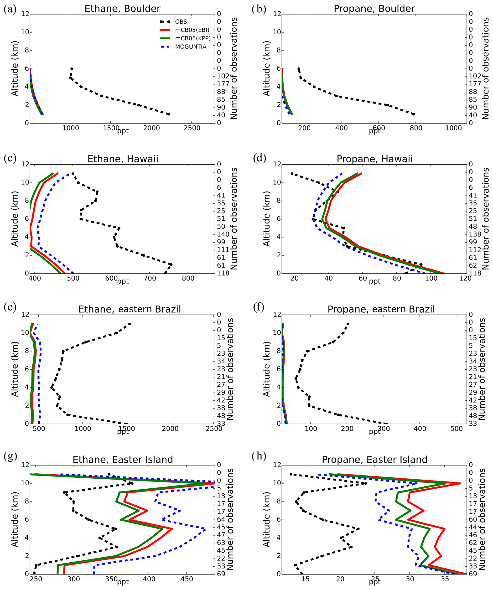
Figure 10 Comparison of TM5-MP vertical profiles (km) of C₂H₆ (left column) and C₃H₈ (right column) against aircraft observations (black line; ppt) for the two chemistry schemes, mCB05(KPP) (green line) and MOGUNTIA (blue line), using colocated model output for 2006 sampled at the measurement times; error bars indicate the standard deviation. For comparison, model results of mCB05 with the EBI solver (red line) are also presented. The numbers on the right vertical axis indicate the number of available measurements.

Propane (C₃H₈) is also emitted mainly from anthropogenic sources, and in the current simulations the total emission is 8.5 Tg yr⁻¹ (Table 3), which is lower compared to other reported emission estimates of ∼ 15 Tg yr⁻¹ (Jacob et al., 2002). Model comparison with flask observations (Fig. 9) shows that the model tends to underestimate the measured mixing ratios for all simulations but with higher correlation coefficients compared to C₂H₆ in most of the cases. C₃H₈ is underestimated in the NH at Mace Head (Fig. 9b) during the winter and autumn seasons by 72 %–74 %. In the tropics, strong negative biases of ∼ 100 ppt are observed at Mauna Loa (Fig. 9d). However, the model simulates the C₃H₈ surface mixing ratios better in the SH at Cape Grim compared to stations in the NH (Fig. 9b, d, f) due to the weaker impact of anthropogenic emissions. In contrast to the C₂H₆ evaluation, however, the model satisfactorily simulates the observed C₃H₈ mixing ratios at the South Pole (Fig. 9h), with a small overestimation during the local summer season. The full set of C₃H₈ comparisons with flask data is presented in Fig. S9. As for the case of C₂H₆, to further investigate the impact of emissions on the simulated C₃H₈ mixing ratios, additional simulations are performed by (1) doubling and (2) quadrupling the anthropogenic fossil fuel emissions, resulting in total C₃H₈ emissions of ∼ 14.9 and ∼ 27.9 Tg yr⁻¹, respectively. The global C₃H₈ tropospheric burdens have been increased by a factor of ∼ 1.7 and 3.2, respectively. Figure S7 indicates that an increase in C₃H₈ emissions by 2 times tends to significantly improve the model simulations, whereas a respective increase by 4 times tends to overestimate the observed mixing ratios.

Figure 11 Comparison of TM5-MP vertical profiles (km) of C₂H₄ (left column) and C₃H₆ (right column) against aircraft observations (black line; ppt) for the two chemistry schemes, mCB05(KPP) (green line) and MOGUNTIA (blue line), using colocated model output for 2006 sampled at the measurement times; error bars indicate the standard deviation. For comparison, model results of mCB05 with the EBI solver (red line) are also presented. The numbers on the right vertical axis indicate the number of available measurements.

Comparison with C₂H₆ and C₃H₈ aircraft climatological data (Fig. 10) further indicates that all chemistry configurations tend to underestimate the observed mixing ratios (∼ 20 %–60 %) in most of the cases, especially in the upper troposphere. In more detail, in Boulder and eastern Brazil, the model significantly underestimates the observed mixing ratios for both compounds, while in Hawaii C₂H₆ is underestimated but C₃H₈ is well simulated by all three configurations. In contrast, at Easter Island, all schemes overestimate the observed mixing ratios for both compounds, although the MOGUNTIA overestimate is larger for C₂H₆ and lower for C₃H₈ compared to the two mCB05 configurations. The full sets of C₂H₆ and C₃H₈ comparisons with aircraft climatological data are presented in the Supplement (Figs. S10 and S11, respectively). Overall, considering that the model reasonably simulates the oxidative capacity of the atmosphere, direct emissions are the likely reason for these differences, since both alkanes are oxidized in the troposphere by OH radicals and no secondary production terms of these alkanes are known. Note, however, that alkane emission fluxes are on the low side, as also reported by other studies (e.g., Aydin et al., 2011; Huijnen et al., 2019; Monks et al., 2018).

5.5.2 Ethene and propene

Ethene is mainly emitted from biogenic sources and by incomplete combustion from biomass burning, power plants, and combustion engines. C₂H₄ emissions in the model are roughly 30 Tg yr⁻¹ (Table 3), close to the estimate of Huijnen et al. (2019) but on the high side compared to the 21 Tg yr⁻¹ reported by Toon et al. (2018). The three chemistry configurations produce similar mixing ratios of C₂H₄ in most of the cases. Nevertheless, the comparison with aircraft observations (Fig. 11) indicates underestimated mixing ratios in the upper troposphere. In more detail, the model reproduces (R=0.97) the vertical distribution of C₂H₄ well in Boulder (USA). However, observed mixing ratios close to the surface (up to ∼ 2 km) are overestimated by the model, while observations at the higher levels (up to ∼ 6 km) are underestimated. In the tropics, the observed mixing ratios in the lower and upper troposphere (e.g., in Hawaii) are slightly overestimated by the model for all configurations, although for the MOGUNTIA configuration this overestimate is the lowest. In remote regions, where the impact of direct emissions is negligible (e.g., at Easter Island), the model overestimates C₂H₄ close to the surface (∼ 1 km), but some negative biases appear aloft. At higher altitudes, however, all configurations overestimate the observed C₂H₄ mixing ratios (Fig. 11g), but again the MOGUNTIA model configuration better reproduces the observations. Overall, these deviations from the observations could be attributed to (1) the background concentrations not being well resolved by the model, (2) the severe uncertainties in emission fluxes, and (3) chemistry that is not well understood (e.g., Huijnen et al., 2019; Pozzer et al., 2007), such as the C₂H₄ production during VOC decomposition in the atmosphere.

Propene (C₃H₆) emissions in the model are ∼ 32 Tg yr⁻¹ (Table 3). The two mCB05 configurations produce similar C₃H₆ mixing ratios, but MOGUNTIA tends to simulate higher values, especially in the tropics, in Hawaii (Fig. 11d), and in eastern Brazil (Fig. 11f). Close to the surface, where the impact of the emissions is stronger, the model severely overestimates observations (Fig. 11d, f), except for Japan (Fig. 11b). For the MOGUNTIA configuration, this overestimation is more substantial in the tropics compared to the mCB05 chemistry scheme. An overestimation of the observed mixing ratio close to the surface is also found in other regions, especially in the SH, such as in eastern Brazil (Fig. 11f), and in remote regions where the direct impact of emissions is negligible, such as Easter Island (Fig. 11h). However, at Easter Island (Fig. 11h), the model fails to reproduce the observed C₃H₆ vertical profile, resulting in a significant underestimation of the observed mixing ratios. Overall, even though the evaluation of vertical profiles should be considered here only as a climatological comparison, the reason for the model underestimation of C₃H₆ mixing ratios at higher altitudes is likely a combination of the emission strengths, the simulated vertical distribution, and the potential but still unaccounted for secondary production from higher VOC oxidation. All comparisons for C₂H₄ and C₃H₆ with aircraft climatological data are presented in Figs. S12 and S13, respectively.

6 Summary and conclusions

This study documents and evaluates the implementation of the tropospheric chemistry scheme MOGUNTIA in the global chemistry and transport model TM5-MP. The MOGUNTIA scheme is a comprehensive gas-phase chemistry mechanism that explicitly accounts for the oxidation of light hydrocarbons, coupled with an updated representation of isoprene oxidation, along with a simplified representation of terpenes and aromatics chemistry. The newly coupled chemistry scheme in TM5-MP is compared to the existing chemistry scheme of the model, mCB05. Another feature implemented in the TM5-MP chemistry code is the Rosenbrock solver that replaces the classical EBI method. For this, a simple preprocessor directive has been implemented in the model to choose between the two solvers during model compilation. In the case of the Rosenbrock solver, the KPP software has been used to generate the chemistry code coupled with the TM5-MP. To further examine the impact of the solver on the TM5-MP atmospheric simulations and performance, the mCB05 scheme is also tested using the Rosenbrock solver.

Global budgets of O₃, CO, and OH, for all simulations performed for this work, are calculated and compared with estimates published in the literature. In more detail, the O₃ budget calculated with the MOGUNTIA chemistry scheme falls within 1 standard deviation of mean estimates from other modeling studies. However, the new MOGUNTIA scheme reduces the tropospheric O₃ burden by ∼ 3 % compared to the mCB05 configurations. For tropospheric CO, a respective reduction in the atmospheric lifetime (∼ 6 %) provides evidence that the implementation of the MOGUNTIA chemistry leads to an increase in the oxidative capacity of the troposphere in TM5-MP. This also holds for the atmospheric CH₄ chemical lifetime that is calculated here to be about 8.0 years for the MOGUNTIA chemistry scheme, which is roughly 3 %–5 % shorter compared to mCB05(KPP) and mCB05(EBI) configurations.

The large-scale variability in space and time of modeled tropospheric NO₂, OH, O₃, CO, and light VOCs (i.e., C₂H₆, C₂H₄, C₃H₈, C₃H₆) has been evaluated for the year 2006 and compared to several sets of in situ observations, satellite retrievals, and climatological data. Overall, both the lumped-structure (i.e., the mCB05) and the lumped-molecule (i.e., the MOGUNTIA) mechanisms appear to be able to satisfactorily represent the tropospheric chemistry. In most of the cases, lower biases compared to measurements are calculated when the MOGUNTIA chemistry configuration is used. The model simulates the major observed features of the spatial and temporal variability well in surface observations for O₃ and CO. The observed background surface O₃ mixing ratios are captured with a bias of ∼ 6.5 ppb for the MOGUNTIA configuration, very close to the mCB05 configurations. Ozone in the vertical matches on average within ∼ 5 ppb for all configurations, and the model is able to capture the variability observed by ozonesondes well. In contrast, the model underestimates the available CO flask observations by roughly 30 % for all configurations, most likely linked to uncertainties in the seasonal cycle of anthropogenic emissions and the representation of biomass burning CO emissions. For the model comparison with observed light VOC mixing ratios, all chemistry configurations clearly show that significant uncertainties still exist regarding their emission strength or poorly understood chemistry, such as secondary chemical production during the decomposition of higher VOCs in the atmosphere. Sensitivity simulations performed indicate that increases in emissions may improve the simulation of the atmospheric mixing ratios of some light VOCs, such as C₃H₈. However, our results suggest that changes in emissions should not just be based on fixing the model's emissions using a specific (constant) value but that scientifically accepted methods should be used. Future studies should therefore aim at improving source estimates and a better understanding of the processes that govern the budgets of light VOCs. From a chemistry point of view, it would be interesting to study the chemical formation pathways from higher VOCs. Inverse modeling or data assimilation studies might also be used to “optimize” the emissions in order to minimize the differences between observations and model simulations.

The presented model configurations result in a benchmark of the TM5-MP tropospheric chemistry version upon which future model improvements may take place. Inherent uncertainties need to be reduced and further work is required, focusing mainly on the most poorly understood chemistry-related processes. For example, further attention concerns the uncertainties in $\mathrm{NO}-{\mathrm{NO}}_{\mathrm{2}}-{\mathrm{O}}_{\mathrm{3}}$ cycling along with the atmospheric fate of ORGNTRs and their impacts on the oxidative capacity of the troposphere. Attention is also needed for the treatment of aerosols and clouds, in particular ice clouds and their impact on photolysis frequencies. Other issues that need to be resolved are related to the significant uncertainties in light hydrocarbon mixing ratios – as clearly seen in the model comparison to surface and aircraft observations – and their potential impact on the oxidative capacity of the troposphere. Considering that both chemistry schemes underestimate light VOC mixing ratios in most of the cases, the use of a more detailed scheme such as MOGUNTIA will allow us to better understand the causes of this deviation compared to the lumped representation of VOC chemistry in the mCB05 mechanism. This is especially relevant over tropical regions with high biogenic VOC emissions under low-NO_x conditions. For this, a more dedicated comparison of the model with in situ observations and satellite retrievals is needed. MOGUNTIA also contains an ample number of oxygenated VOCs that are observed in the atmosphere at significant levels and further involved in aerosol formation, making the scheme appropriate for detailed studies. On top of this, the implementation of the KPP software in the model makes the code a lot more flexible for chemistry updates compared to the previous EBI-based chemistry versions. The use of the KPP in TM5-MP reduces the uncertainties in solving stiff chemistry equations and opens up new possibilities for model development, such as the construction of an adjoint of the chemistry mechanism that can be used in 4D-Var data assimilation systems (e.g., Henze et al., 2007). Another possible application is to more accurately explore atmospheric chemistry–climate interactions, since TM5-MP is also coupled to the Earth System Model EC-Earth (e.g., Van Noije et al., 2014). Note, however, that despite the clear benefits regarding code development and management, the use of a more sophisticated solver such as the Rosenbrock solver and the implementation of a detailed chemistry scheme such as MOGUNTIA make the code computationally more expensive. Overall, this work shows that the newly coupled chemistry version of TM5-MP works as well as – or better than in some cases – the previous chemistry versions of the model, opening opportunities for further chemistry developments and more detailed tropospheric investigations by the TM and EC-Earth communities.