Description and evaluation of the process-based forest model 4C v2.2 at four European forest sites

The process-based model 4C (FORESEE) has been developed over the past 20 years to study climate impacts on forests and is now freely available as an open-source tool. The objective of this paper is to provide a comprehensive description of this 4C version (v2.2) for scientific users of the model and to present an evaluation of 4C at four different forest sites across Europe. The evaluation focuses on forest growth as well as carbon (net ecosystem exchange, gross primary production), water (actual evapotranspiration, soil water content), and heat fluxes (soil temperature) using data from the PROFOUND database. We applied different evaluation metrics and compared the daily, monthly, and annual variability of observed and simulated values. The ability to reproduce forest growth (stem diameter and biomass) differs from site to site and is best for a pine stand in Germany (Peitz, model efficiency ME=0.98). 4C is able to reproduce soil temperature at different depths in Sorø and Hyytiälä with good accuracy (for all soil depths ME > 0.8). The dynamics in simulating carbon and water fluxes are well captured on daily and monthly timescales (0.51 < ME < 0.983) but less so on an annual timescale (ME < 0). This model–data mismatch is possibly due to the accumulation of errors because of processes that are missing or represented in a very general way in 4C but not with enough specific detail to cover strong, site-specific dependencies such as ground vegetation growth. These processes need to be further elaborated to improve the projections of climate change on forests. We conclude that, despite shortcomings, 4C is widely applicable, reliable, and therefore ready to be released to the scientific community to use and further develop the model.

1 Introduction

Forest modelling has a long tradition in forest science and ecology, and it is of central importance to understanding forest functioning and dynamics, as well as for planning forest management and assessing forest product and service provisioning (Pretzsch, 2010). While climate change impact studies often emphasize long-term forest development, nowadays changes in environmental conditions have provoked a wider interest in the sustainability of various forest ecosystem services. There is also an increasing demand for estimating the sensitivity of forests to disturbance events as well as elucidating forest management options to mitigate climate change. These challenges require accounting for a high degree of complexity in forest ecosystems and thus demand forest models that can capture numerous interactions between air, soil, and vegetation. For this reason, stand-scale process-based forest models (PBMs) have been developed over the past 30 years that try to explain forest growth and development based on ecological understanding (Fontes et al., 2010; Landsberg, 2003; Mäkelä et al., 2000a; Medlyn et al., 2011). These models can be stand-based or individual-based, and many of these models are used to study climate change impacts on forest productivity (see review by Reyer, 2015) , matter dynamics (water, carbon, nitrogen) (Cameron et al., 2013; Constable and Friend, 2000; Kramer et al., 2002), or the effects of forest management (Fontes et al., 2010; Porte and Bartelink, 2002; Pretzsch et al., 2008). These models typically operate at stand scale and yet include similar process detail as land surface models (Fisher et al., 2015; Naudts et al., 2015) that are typically applied to larger scales. They can also be applied to larger spatial scales but typically without considering interactions among landscape patches, as opposed to landscape models that place particular emphasis on the processes connecting different patches of forests such as dispersal or propagation of disturbances (Seidl et al., 2012). One such model is the forest model “FORESt Ecosystems in a changing Environment”, called FORESEE in short form and 4C in even shorter form, developed at the Potsdam Institute for Climate Impact Research in Germany.

The development of the forest model 4C started in the 1990s (Bugmann et al., 1997) at a time when environmental change, especially climate change, had been hypothesized to provoke major changes in forest ecosystems that could not be covered by traditional, statistical forest models. Therefore, the main idea was to develop a forest model that describes individual forest stands and has the following characteristics:

• it represents our knowledge of the main mechanisms of forest functioning such as photosynthesis, allocation, and water relations (i.e. is process-based);

• it is responsive to changing environmental conditions;

• it is generic in its structure; and

• it is applicable to forests worldwide.

The model's objectives include scenario analyses regarding (i) impacts of climate change and other changing environmental conditions (e.g. CO₂, N deposition) on forest growth and matter balance (carbon, water, nitrogen), (ii) effects of forest management on forest ecosystem functioning, and (iii) impacts of biotic disturbances on forest growth.

The concept underlying 4C and its salient features were outlined by Bugmann et al. (1997) and individual processes of the model by Lasch et al. (2002, 2005) and Reyer et al. (2010). However, a full description of the model has never been officially published and since the model version 4Cv2.2 has recently been published as an open-source tool in a Gitlab repository (https://gitlab.pik-potsdam.de/foresee/4C, last access: 30 October 2020), we present the model in more detail and illustrate its main features with model runs compared to observed data using the PROFOUND database (Reyer et al., 2019, 2020). We use the PROFOUND database for two main reasons: (1) the PROFOUND database provides a wide range of data for evaluation and allows us to compare model simulations against stand growth as well as carbon, water, and heat flux data. (2) The database is also currently the basis for a forest model intercomparison within the framework of the Intersectoral Model Intercomparison Project (https://www.isimip.org/, last access: 30 October 2020), and hence not only 4C will be evaluated at these sites but also a range of other models.

Therefore, the main objectives of this paper are the following:

1. to provide a comprehensive description of the structure and the processes of the recently open-sourced version 2.2 of 4C (Lasch-Born et al., 2019);

2. to evaluate the model's performance in reproducing growth, carbon and water fluxes, soil temperature, and water content for typical European forest stands with data from the PROFOUND database; and

3. to discuss the general applicability of the model and to highlight potential future improvements for scientific users of the open-source version of the model.

This paper and its accompanying detailed model description and Gitlab repository target scientists that are interested in applying and developing complex forest stand models without necessarily wanting to start building the model from scratch but building on an established model that has been widely applied and can be adjusted to their needs. Therefore, besides the detailed model description and evaluation, we also provide hints on how to best apply and use the model throughout the text.

2 Methods

2.1 Model 4C

In the following, we briefly present the main features of 4Cv2.2. More details on all processes, state variables, and parameterizations are given in an extensive model description (Lasch-Born et al., 2018) and also on the model's website: http://www.pik-potsdam.de/4c/ (last access: 30 October 2020). Version 2.2 differs from its predecessors by a variety of model extensions and revisions. Amongst others, we enlarged the number of species and species parameters, included new management methods (e.g. short-rotation coppice), revised the calculation of the effect of nitrogen availability on growth, and implemented the effects of biotic disturbances on stand dynamics.

2.1.1 Overview

4C describes tree species composition, forest growth and structure, and the whole carbon, water, and nitrogen balance of a forest stand on an area basis. It can be applied for patches of various sizes (varying from 100 m² to several hectares) and mono- and mixed-species forests. The model mechanistically describes forest responses to climate, nitrogen, and CO₂, and it accounts for realistic representation of forest management (Bugmann et al., 1997; Lasch et al., 2005). A forest stand is represented by a number of tree cohorts, each of which contains a specific number of trees. All trees within a cohort share the same characteristics, which are species, age, tree dimensions (height, height of crown base or bole height, and diameter at breast height), biomass differentiated into various compartments (foliage, fine roots, sapwood, and heartwood), and stage of phenological development. This allows simulating a representative tree of each cohort instead of each tree in the stand. The model is distance-independent, trees within a cohort are horizontally evenly distributed, and their position unknown. There are no differences in the growth behaviour of the trees of a cohort and there is no competition between the trees within a cohort. In contrast, the tree cohorts compete for light, water, and nutrients. Their relative success in this competition determines their performance in terms of growth and mortality. Establishment of new cohorts is simulated with a regeneration module. The vertical structure of the crown space and rooting zone is represented by a resolution into vertical layers. The model requires the following input data: daily meteorological data, a detailed description of the physical and chemical characteristics of each soil layer, and an initialization of cohort properties (see Sect. 2.1.4).

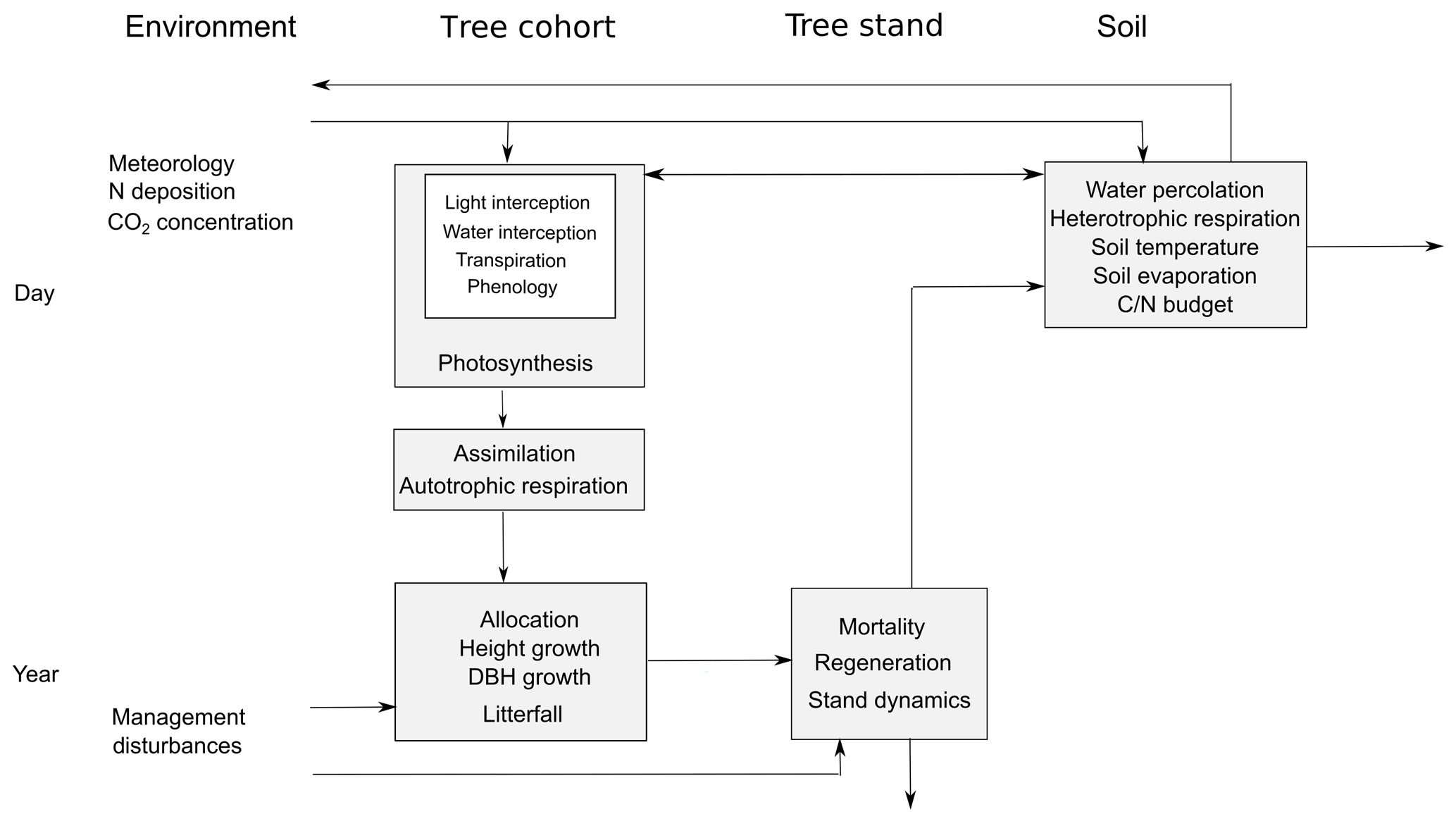
Figure 1 Structural scheme of the 4C model. The individual processes are listed according to the associated model component (horizontally) and their temporal resolution (vertically), the arrows describe information and material fluxes, and the boxes assemble processes on the same temporal or spatial level.

Different timescales are used for the submodels, ranging from a daily time step for e.g. soil water dynamics and phenology, to a weekly time step for photosynthesis (based on weekly averaged daily climate data), and to an annual time step for tree carbon allocation, dimensional growth, and mortality (Fig. 1).

Physiologically based and empirical functions were selected and implemented in 4C to provide an understanding of forest functioning that is as general but also as simple as possible (law of parsimony; Coelho et al., 2019). As an example, the empirical relationship between foliage mass and height used in the model is described with one single function that uses only three species-specific parameters (see Sect. 2.1.3, Eq. 13). This function was selected after analysing the general applicability across species and simple species-specific parameter estimation. Another example is the reduction of the number of parameters in the soil temperature model of 4C. Analyses showed that it is sufficient to use the air temperature of the last 3 d for the calculation of the surface temperature of the ground and to determine the corresponding three parameters (Suckow, 1985). It should also be noted that the temporal resolutions of process descriptions are selected specifically for medium- and long-term analyses (from 1 year up to several hundred years). Therefore, a coarser resolution is preferred for processes such as allocation that may vary at short timescales but still obey general rules in the longer term.

For several key processes, 4C provides alternative descriptions to enable an uncertainty analysis across different model assumptions or for selecting processes at different levels of detail depending on data availability for parameterization or stand initialization. For example, evapotranspiration can be calculated using approaches by Turc and Ivanov (Dyck and Peschke, 1995; DVWK, 1996), Penman–Monteith (Monteith and Unsworth, 1990), or Priestley–Taylor (Priestley and Taylor, 1972). Each of these process descriptions is suited for different applications. The Turc–Ivanov procedure is a simple estimate which requires the least input data, whereas Penman–Monteith uses a full range of meteorological variables and is based on physical knowledge, which allows for more precise estimates of evapotranspiration (Kingston et al., 2009). Hence, 4C is not only a forest model but also a forest modelling framework (for details see, Lasch-Born et al., 2018).

2.1.2 Tree species parameterization

4C is parameterized for the most common European tree species: common beech (Fagus sylvatica L.), Norway spruce (Picea abies L. Karst.), Scots pine (Pinus sylvestris L.), oaks (Quercus robur L. and Quercus petraea Liebl.), and birch (Betula pendula Roth). In addition, parameters for some species that are considered favourable under expected environmental changes or that are used for short-rotation coppices have also been tested and are readily applicable. The considered species include Douglas fir (Pseudotsuga menziesii (Mirb.) Franco), black locust (Robinia pseudoacacia L.), Aleppo pine (Pinus halepensis Mill.), eucalyptus (Eucalyptus globulus Labill. and Eucalyptus grandis W. Hill ex Maiden), and poplars (Populus tremula (L.), P. tremuloides (Michx.)). Moreover, parameter sets for Ponderosa pine (Pinus ponderosa Dougl.) and lodgepole pine (Pinus contorta Dougl.) exist but have not been properly tested. The oak, eucalypt, and poplar parameters are derived from investigations of two species of the same genus each and are assumed to be valid for both. Besides these tree species, 4C is also parameterized for the hemiparasitic plant mistletoe (Viscum album subsp. austriacum) and a generic grassy ground vegetation based on properties of Calamagrostis arundinacea. For each species, there is a maximum of 95 parameters which are needed to cover all processes available in the 4C modelling framework (see Sect. 2.1.1). Depending on which processes (e.g. which of the evapotranspiration submodels) are finally included in a simulation, the minimum set of required parameters is 40. Not all parameters differ across species yet, but they can potentially be varied further if relevant scientific evidence becomes available. The values and descriptions of the parameters are available in Lasch-Born et al. (2018).

The philosophy of 4C is to rely on processes as close as possible to the underlying principles of forest growth, demography, carbon and water cycling, and heat transport. Covering the most important of such processes, one parameter set for each species can be chosen that reproduces species growth, water, and carbon cycling under a wide range of environmental constraints and hence can be kept fix over time and space without need for calibration. Therefore, the values of the 4C parameters were derived from the scientific literature, by expert knowledge, or from other published models. If a variety of values were found in this way, the value set for 4C was determined through detailed testing and sensitivity analyses (not published). Therefore, recalibration of the species-specific parameters is not necessary when setting up the model for a new site but is of course possible if data are available and a recalibration is required to achieve the aims of the study.

In recent years, more and more evidence has accumulated that different physiological parameters have been determined in different environments (Kattge et al., 2020) or are dependent on stand density or site fertility (e.g. Berninger et al., 2005). To address these issues of parameter uncertainty, we have tested calibrating 4C in systematic Bayesian calibration studies (van Oijen et al., 2013; Reyer et al., 2016). The main goal of these studies was to analyse effects of parameter uncertainty on simulated net primary production (NPP) and forest growth. Reyer et al. (2016) used uniform priors for 42 parameters varying by ± 25 % and 50 % around their standard value and data from different Scots pine stands throughout Europe to calibrate 4C. The different calibrations showed that even though the output uncertainty induced by the parameter variations is large when projecting climate impacts on NPP, Bayesian calibration in the historical period reduced those uncertainties. Most importantly, these tests showed that the direction of NPP change is mostly consistent between the simulations using the uncalibrated standard parameter setting of 4C and the majority of the simulations including parameter uncertainty. Following a similar simulation set-up but examining results in a multi-model context, 4C was found to be the most plausible out of six established forest models (van Oijen et al., 2013).

2.1.3 Main processes and submodels

Light competition

The cohorts compete for light, and the fraction of photosynthetically active radiation absorbed by each cohort is calculated based on the Lambert–Beer law (Haxeltine and Prentice, 1996b; Monsi and Saeki, 2005).

The absorbed photosynthetically active radiation I_PAR is the fraction of global radiation R_g, which is not reflected by the albedo α_refl:

$$\begin{array}{}\text{(1)}& I_{\text{PAR}}={\mathit{\alpha }}_{\text{refl}}{\mathit{\eta }}_{\mathrm{R}}{R}_{\mathrm{g}},\end{array}$$

where η_R is a factor which converts the incident radiation from joules per square centimetre (J cm⁻²) to moles per square metre (mol m⁻²) under the assumption that only 50 % of incident radiation is photosynthetically active. The share of any cohort in the total stand's net photosynthetic assimilation of carbon is proportional to its share of the absorbed photosynthetically active radiation I_PAR. The total fraction $f_{\text{tot}}^c$ of I_PAR absorbed by each cohort c is calculated each time stand phenology changes based on the Lambert–Beer law. There are four different models to calculate light transmission and absorption through the canopy, abbreviated as LM1, LM2, LM3, and LM4 in Lasch-Born et al. (2018). Whereas LM1 is based on the classical gap model approach that each tree covers the whole patch with its canopy, this simplistic view is refined in LM2 by attributing each cohort or tree c a specific projected crown coverage area $a_{\text{cr}}^c$ depending on its d_bh. LM2 and LM3 differ in the way the light is transmitted through the canopy, and LM4 additionally introduces an average growing season sun inclination angle β.

Every time phenology changes within the stand, e.g. a species has its bud burst or leaves are colouring, the light transmission through the canopy and accordingly light absorption changes. First, the light routines of the 4C model calculate the leaf area for each cohort $c=\mathrm{1},\mathrm{\dots },n_c$ and each canopy layer $j=\mathrm{0},\mathrm{\dots },n_l$ (l_a,c(j)), respectively, based on the leaf biomass M_f available per year and cohort, total height, and height of crown base. This is achieved using a leaf area–leaf dry mass relationship. Because this species-specific leaf area (SLA) varies within the canopy from sun to shade leaves, an average SLA ($s_{\text{av}}^c$) is calculated per cohort c depending on the average relative light regime in the cohort's canopy of the previous year:

$$\begin{array}{}\text{(2)}& s_{\text{av}}^c=s_{\text{min}}^c+s_{\mathrm{a}}^c\left(\mathrm{1}-{\displaystyle \frac{i_c\left(n_l\right)+i_c\left(\mathrm{1}\right)}{\mathrm{2}}}\right),\end{array}$$

where $s_{\text{min}}^c$ denotes the minimal SLA per cohort c, as it is usually found in sun leaves at the top of the canopy, and $s_{\mathrm{a}}^c$ stands for the slope with which $s_{\text{av}}^c$ rises according to the average light regime. The calculation of the relative light intensity i_c(j) available in layer j for cohort c depends on the light model and is described below. The $s_{\text{av}}^c$ rises with increasing depth of the cohort's canopy. The $s_{\mathrm{a}}^c$ can be approximated when the SLA of shade leaves ($s_{\text{max}}^c$) and the SLA of sun leaves $s_{\text{min}}^c$ are known by

$$\begin{array}{}\text{(3)}& s_{\text{max}}^c=s_{\text{min}}^c+\mathrm{0.5}{s}_{\text{av}}^c.\end{array}$$

It has to be noted, however, that the average light regime as calculated in Eq. (3) is higher than the relative light in the middle of the canopy because of the concave nature of the light extinction curve; it is also usually not 0.5.

All approaches mentioned above calculate the absorbed photosynthetically active radiation for each cohort in each layer of the canopy between the height and bole height of the trees, but they differ in the way light is transmitted through the canopy and in the consideration of sun inclination (see Lasch-Born et al., 2018). The daily total radiation absorbed by the canopy is mainly used for calculating photosynthesis and potential evapotranspiration.

Phenology

For deciduous tree species, 4C models bud burst to determine the start of the vegetation period. Bud burst is calculated according to three different approaches driven by temperature and photoperiod (day length) as described by Schaber (2002) and Schaber and Badeck (2003). The most frequently used approach is the promotor–inhibitor model (PIM) that is based on simple interactions between inhibitory and promoting agents that are assumed to control the developmental status of a plant. The abundance or concentration of certain enzymes in cells is determined by the rates of synthesis and breakdown. Control of these processes is the subject of a lot of research; however, it is known that temperature and photoperiod play a prominent role. Temperature, for instance, can act through pure physical mechanisms like its influence on viscosity and diffusion. Moreover, synthesis of proteins usually has activation energy or temperature and an optimal temperature beyond which synthesis rates decrease again (Vegis, 1973; Johnson and Thornley, 1985). Photoperiod has been observed to be the driving force of a biochemical trigger acting through the photochromic system (Wareing, 1956; Perry, 1971; Nitsch, 1957; Heide, 1993b, a). From these simple but basic principles a model for the abundance or concentration of an inhibitory compound I_phen and a promoting compound P_phen can be formulated as a system of two simple coupled difference equations:

$$\begin{array}{}\text{(4)}& \begin{array}{rl}& \mathrm{\Delta }{I}_{\text{phen}}=p_{\mathrm{1}}{f}_{\mathrm{1}}\left(T\right)g_{\mathrm{1}}\left(d_{\mathrm{l}}\right)-p_{\mathrm{2}}{f}_{\mathrm{2}}\left(T\right)g_{\mathrm{2}}\left(d_{\mathrm{l}}\right)I_{\text{phen}},\\ & \mathrm{\Delta }{P}_{\text{phen}}=p_{\mathrm{3}}{f}_{\mathrm{3}}\left(T\right)g_{\mathrm{3}}\left(d_{\mathrm{l}}\right)(\mathrm{1}-I_{\text{phen}})-p_{\mathrm{4}}{f}_{\mathrm{4}}\left(T\right)g_{\mathrm{4}}\left(d_{\mathrm{l}}\right)P_{\text{phen}},\end{array}\end{array}$$

where p_i represents scaling parameters, and f_i, g_i, and $i=\mathrm{1},\mathrm{\dots },\mathrm{4}$ are functions of air temperature T_a and photoperiod (day length) d_l, respectively. Temperature T_a and photoperiod d_l are themselves functions of time, in our case of the day of the year. Breakdown of the compounds P_phen and I_phen, indicated by the negative terms in Eq. (4), is assumed to be a first-order reaction, whereas the synthesis terms, indicated by the positive terms in Eq. (4), are formulated as simple forcing terms. The synthesis term of the promotor P_phen is coupled to or is rather damped by the presence of the inhibitor I_phen. P_phen and I_phen are normalized arbitrarily to vary between 1 and zero. For each species the PIM determined which model formulations best suited the observed dates of bud burst (BB) and corresponding course of temperature and day length. For more details see chapter 4.1 in Lasch-Born et al. (2018).

The second implemented and parameterized model is the Cannel and Smith model (CSM) that empirically describes the observation that increased chilling in winter decreases the required temperature sum for bud burst in spring. It was developed by Cannell and Smith (1983) and modified by Menzel (1997); see chapter 4.1.2 in Lasch-Born et al. (2018).

The also implemented temperature sum model (TSM) (Menzel, 1997; Wang, 1960; Kramer, 1994) simply integrates daily mean temperatures T_a above a certain threshold T_b starting from a defined date t₁ up to a fixed critical value T_crit.

The date of leaf fall is fixed. For coniferous tree species the length of the vegetation period is 1 year.

Production, allocation, and growth

The annual course of net photosynthesis and net primary productivity is simulated for each cohort with a mechanistic formulation of net photosynthesis as a function of environmental influences (temperature, water and nitrogen availability, radiation, and CO₂). The approach for the photosynthesis is based on the mechanistic photosynthesis model of Farquhar et al. (1980) as simplified by Collatz et al. (1991) wherein the physiological capacity (maximal carboxylation rate) is calculated based on optimization theory (modified after Haxeltine and Prentice 1996b, a).

This approach is used to calculate the daily net photosynthesis A_dt and the leaf maintenance respiration R_d of a tree. The model applied has the important feature that the resulting net photosynthesis is a linear function of the photosynthetically active radiation I_PAR (see Sect. 2.1.3). Given this linearity, it is not necessary to integrate photosynthesis explicitly across the canopy, but it is sufficient to calculate the total radiation absorbed by the canopy and then to calculate the total daily net photosynthesis A_nd as a function of the absorbed radiation f(I_PAR) that results for the whole canopy at once.

The total amount of optimum gross (nitrogen limited) assimilation per tree or cohort A_c is then obtained by

$$\begin{array}{}\text{(5)}& A_{\mathrm{c}}=A_{\text{sp}}{\displaystyle \frac{P_a}{\mathrm{1000}}}{\displaystyle \frac{\mathrm{1}}{c_{\text{part}}}},\end{array}$$

where P_a is patch size (m²), A_sp is the specific gross photosynthesis rate, and c_part is the part of carbon in biomass used to convert A_sp from carbon to dry weight (DW). The factor 1000 converts A_sp ($\mathrm{g}\mathrm{C}{\mathrm{m}}^{-\mathrm{2}}{\mathrm{d}}^{-\mathrm{1}}$) from grams to kilograms. A_c thus is in kilograms of dry weight per square metre per day ($\mathrm{kg}\mathrm{DW}{\mathrm{m}}^{-\mathrm{2}}{\mathrm{d}}^{-\mathrm{1}}$).

The rate A_sp is calculated from the (nitrogen-limited) light use efficiency L_UE (g C µmol⁻¹), the daily incident photosynthetic radiation I_PAR (mol m⁻²), and the fraction of absorbed photosynthetically active radiation $f_{\text{tot}}^c$ (–) per cohort.

$$\begin{array}{}\text{(6)}& A_{\text{sp}}=L_{\text{UE}}{f}_{\text{tot}}^c{I}_{\text{PAR}}\end{array}$$

L_UE is derived from the optimal light use efficiency L_UE,opt (Haxeltine and Prentice, 1996b) reduced by a reduction factor $R_{\mathrm{N}}^c$, which describes the influence of nitrogen availability calculated as a function of the C∕N ratio of the soil, the ratio of the plant's nitrogen demand and availability, and the species-specific photosynthesis response to nitrogen (see chapter 3.5 in Lasch-Born et al., 2018):

$$\begin{array}{}\text{(7)}& L_{\text{UE}}=R_{\mathrm{N}}^c{L}_{\text{UE,opt}}\end{array}$$

Using the specific daily leaf respiration R_ds ($\mathrm{g}{\mathrm{m}}^{-\mathrm{2}}{\mathrm{d}}^{-\mathrm{1}}$), calculated according to Haxeltine and Prentice (1996a), the nitrogen -limited daytime photosynthesis A_dt (g C m⁻²) is calculated by

$$\begin{array}{}\text{(8)}& A_{\text{dt}}=A_{\text{sp}}-{\displaystyle \frac{d_{\mathrm{l}}}{\mathrm{24}}}{R}_{\text{ds}},\end{array}$$

with the daily length of photoperiod d_l.

This photosynthesis rate is related to the unstressed stomatal conductance of the tree through the CO₂ diffusion gradient between the atmosphere and intercellular air space, and g^c is calculated according to Haxeltine and Prentice (1996a):

$$\begin{array}{}\text{(9)}& g^c=max\left(g_{\text{min}},{\displaystyle \frac{\mathrm{1.56}{A}_{\text{dt}}}{(\mathrm{1}-\mathit{\lambda })c_{\mathrm{a}}{c}_{\text{mass}}}}\right),\end{array}$$

where the factor 1.56 accounts for the difference in the diffusion coefficients of CO₂ and water vapour, $\mathit{\lambda }=c_i/c_{\mathrm{a}}=\mathrm{0.7}$ is the optimum ratio of ambient to intercellular CO₂ concentration, and g_min is the minimum conductance (e.g. due to cuticular transpiration). The division of A_dt by c_mass is required for the conversion of its unit from grams of carbon per square metre per day ($\mathrm{g}\mathrm{C}{\mathrm{m}}^{-\mathrm{2}}{\mathrm{d}}^{-\mathrm{1}}$) into moles of carbon dioxide per square metre per day ($\mathrm{mol}{\mathrm{CO}}_{\mathrm{2}}{\mathrm{m}}^{-\mathrm{2}}{\mathrm{d}}^{-\mathrm{1}}$).

Summation over all cohorts yields the stomatal conductance of the canopy of the stand g_tot.

The realized net daily (water and nitrogen limited) assimilation rate A_net is then calculated by

$$\begin{array}{}\text{(10)}& A_{\text{net}}=I_{\text{drps}}^c(A_{\mathrm{c}}-R_{\text{dc}}),\end{array}$$

where $I_{\text{drps}}^c$ is the water limitation of the photosynthesis calculated per cohort by the ratio of cohort water supply and cohort transpiration demand (see chapter 4.2.3 in Lasch-Born et al., 2018), A_c is the gross assimilation per patch (see Eq. 5), and the daily leaf respiration rate R_dc per patch is defined by

$$\begin{array}{}\text{(11)}& R_{\text{dc}}=R_{\text{ds}}{\displaystyle \frac{P_a}{\mathrm{1000}}}{\displaystyle \frac{\mathrm{1}}{c_{\text{part}}}},\end{array}$$

with the parameter c_part, which gives the part of C in biomass.

Finally, the daily net primary production f_NPP is

$$\begin{array}{}\text{(12)}& f_{\text{NPP}}=A_{\text{net}}(\mathrm{1}-r_{\text{co}}),\end{array}$$

where r_co is the (growth) respiration coefficient following the concept of constant annual respiration fraction as proposed by Landsberg and Waring (1997). The total daily NPP of the stand f_NPP is summarized over all trees of the cohort, over all cohorts of the forest stand, and over all days and weeks of the year to an annual net primary production of the stand.

The nitrogen content in the tree results from constant species-specific C∕N ratios separated for fine and coarse roots, twigs and branches, stem, and foliage. The C∕N contents are used to calculate the nitrogen demand of the tree and interact with the soil, vegetation, and atmosphere due to its influence on the mineralization of the plant litter (see below).

The competition of cohorts for water and nutrients is modelled via absorption of water and nitrogen by the fine roots in proportion to the fine root mass of the individual cohorts in a specific soil layer. Elevated CO₂ affects photosynthesis through an increase in the internal partial pressure of CO₂, which increases light use efficiency and gross assimilation and reduces stomatal conductance as well as the potential water demand for transpiration. Therefore, water use efficiency is increased with increasing CO₂ (Haxeltine and Prentice, 1996a).

The total tree, cohort, and stand respiration is calculated as a constant annual fraction of gross primary productivity (GPP) as proposed by Landsberg and Waring (1997). Therefore, the net primary production (NPP) is also a constant fraction of GPP (Waring et al., 1998).

The allocation of annual net primary productivity to different tree organs (sapwood, heartwood, foliage, and fine root biomass) and dimensional tree growth is modelled by combining the pipe model theory (Shinozaki et al., 1964), the functional balance hypothesis (Davidson, 1969), and ideas presented by Mäkelä (1990) to make the model sensitive to resource availability and varying demand with increasing dimensions. The detailed derivation of the allocation parameters is given in chapter 4.4 of Lasch-Born et al. (2018)

Height growth is coupled to the growth of the foliage mass and depends on the shading of the crown (Reyer et al., 2010). Based on this relationship for height H,

$$\begin{array}{}\text{(13)}& H={\displaystyle \frac{p_{\text{hv1}}}{p_{\text{hv3}}+(M_{\mathrm{f}}{)}^{p_{\text{hv2}}}}},\end{array}$$

with the three parameters p_hv1, p_hv2, and p_hv3 as well as foliage mass M_f. The parameters were derived from a variety of datasets with available tree height and foliage mass.

The diameter is calculated annually after allocation of NPP and height growth using the sapwood and heartwood area and the length of sapwood pipes. For more details, see Lasch-Born et al. (2018).

Mortality and senescence

Cohort mortality is described on an annual timescale, and two kinds of mortality are considered. The so-called “age-related” mortality is based on tree life span and corresponds to the intrinsic mortality described by Botkin (1993). In addition, the reduction of the number of trees due to limitation of resources and resulting growth suppression is described as carbon-based stress mortality according to Keane et al. (1996). If a tree cohort is not able to reproduce foliage biomass losses within a year, this period counts as a stress year. Successive stress years increase the probability of mortality. Stress-related mortality is species-specific, since the sensitivity to stress years is directly related to the parameterized shade tolerance (see Lasch-Born et al., 2018) of a tree species as well as the abundances of disturbances (see Sect. 2.1.3); see also Lasch-Born et al. (2018). Both types of mortality can be combined or applied separately. Additionally, tree mortality can be superimposed by prescribed mortality events originating from thinning or harvests (see also Sect. 2.1.3)

Annual senescence rates for the biomass compartments foliage, fine roots, and sapwood of a cohort are species-specific and calculated from the corresponding fixed parameterized relative senescence rates. They deliver the litter input to the soil and the transformation of sapwood in heartwood.

Water balance

The following processes are considered for the calculation of the water balance: interception of precipitation, actual evapotranspiration, percolation, and snowmelt. Snowmelt is estimated from the actual air temperature greater than a threshold temperature with a linear approach suggested by Koitzsch and Günther (1990). Intercepted water from the canopy and the ground vegetation is calculated depending on the leaf area and a species-specific interception capacity (Jansson, 1991). The potential evapotranspiration (PET) that is needed to define the evaporation demand of the forest stand is calculated by the approaches of Turc and Ivanov from air temperature and global radiation or relative humidity, respectively (Dyck and Peschke, 1995; DVWK, 1996; Lasch-Born et al., 2015). Further approaches (i.e. Penman–Monteith, Priestley–Taylor) can be selected and are described in more detail in Lasch-Born et al. (2018). The potential evapotranspiration limits the evaporation demand of intercepted and soil water as well as the transpiration of trees and ground vegetation. The actual water uptake of each cohort depends on its transpiration demand and the available water in the soil layers, which is proportional to its relative share of fine roots in each soil layer. The potential canopy transpiration demand E_trd is calculated from the potential evapotranspiration E_pot reduced by the evaporation of intercepted water E_int and the unstressed stomatal conductance g_tot of the forest canopy (Haxeltine and Prentice, 1996a):

$$\begin{array}{}\text{(14)}& E_{\text{trd}}\left(t\right)=\left(E_{\text{pot}}\left(t\right)-E_{\text{int}}\left(t\right)\right){\mathit{\alpha }}_{\mathrm{m}}\left(\mathrm{1}-e^{-\frac{g_{\text{tot}}\left(t\right)}{g_{\text{max}}}}\right),\end{array}$$

with the Priestley–Taylor coefficient α_m and the maximum stomatal conductance g_max. The unstressed stomatal conductance of the canopy g_tot ($\mathrm{mol}{\mathrm{m}}^{-\mathrm{2}}{\mathrm{d}}^{-\mathrm{1}}$) is calculated as the sum of the stomatal conductances of all trees of all cohorts. The stomatal conductance of a single tree in a cohort is calculated according to Haxeltine and Prentice (1996a) from the net daytime photosynthesis A_dt using Eq. (9).

Soil physics, carbon, and nitrogen

The transport of heat and water in multi-layered soil is explicitly calculated, as are carbon and nitrogen dynamics based on the decomposition and mineralization of organic matter (Grote and Suckow, 1998; Grote et al., 1998; Kartschall et al., 1990). The soil of a forest stand is divided into different layers with optional thickness defined based on the horizons of the soil profile. Each layer, including the humus layer and the deeper mineral layers, is assumed to be homogeneous concerning its physical parameters. The water content (W_s – water content per layer, $W_s^{\text{FC}}$ – field capacity) and soil temperature of each soil layer are estimated as functions of soil parameters, air temperature, and stand precipitation. A percolation model balances the soil water content of each layer with depth z and time step t.

$$\begin{array}{}\text{(15)}& \begin{array}{rl}{\displaystyle \frac{\mathrm{d}}{\mathrm{d}t}}\left(W_s(z,t)-W_s^{\text{FC}}\left(z\right)\right)=& W_{\mathrm{p}}(z,t)-W_{\text{upt}}(z,t)-W_{\text{ev}}(z,t)\\ & -{\mathit{\lambda }}_W\left(z\right){\left(W_s(z,t)-W_s^{\text{FC}}\left(z\right)\right)}^{\mathrm{2}}\end{array}\end{array}$$

The percolating water W_p from the above layer serves as input into the soil layer, and the net precipitation after canopy interception serves as input into the first layer. The output is estimated from the soil evaporation W_ev, the water uptake by roots W_upt, and the outflow of gravitational water into the next layer, which is controlled by a soil-texture-dependent percolation parameter λ_W (Glugla, 1969; Koitzsch, 1977).

The water content and soil temperature of each soil layer control the decomposition and mineralization of organic matter. The carbon and nitrogen dynamics are driven by the litter input, which is separated into five fractions for each species (stems, twigs and branches, foliage, fine roots, and coarse roots). The turnover of all litter fractions and of the soil organic matter compartment is described as a first-order reaction (Grote and Suckow, 1998; Post et al., 2007). These processes are controlled by matter- and species-specific reaction coefficients and modified by soil moisture, temperature, and pH value.

The amounts of nitrogen and carbon from litter (needle and foliage litter, twigs, branches, and stems) entering the soil are added to the N and C pools of the primary organic matter of the first layer. In the same way, the nitrogen and carbon content of dead fine and coarse roots of trees as well as ground vegetation is added to the primary organic matter pools (C_pom, N_pom) of the respective soil layer z. The primary organic matter of all species types decomposes to a single humus pool (active organic matter; C_aom, N_aom) for all matter fractions i and species types j. Depending on the carbon and nitrogen content of the organic matter pools and the matter-specific reaction coefficients (k_pom, k_aom), the carbon pools in the soil are estimated in a system of linked differential equations. Mineralized carbon from the active organic matter (heterotrophic respiration) goes back to the atmosphere as CO₂:

$$\begin{array}{}\text{(16)}& {\displaystyle \frac{\partial }{\partial t}}{{\mathrm{C}}_{\mathrm{pom}}}^{i,j}(z,t)=-k_{\text{pom}}^{i,j}{{\mathrm{C}}_{\mathrm{pom}}}^{i,j}(z,t),\text{(17)}& {\displaystyle }\begin{array}{rl}{\displaystyle \frac{\partial }{\partial t}}{\mathrm{C}}_{\mathrm{aom}}(z,t)=& \sum _{i,j}{k}_{\text{syn}}^{i,j}{k}_{\text{pom}}^{i,j}{{\mathrm{C}}_{\mathrm{pom}}}^{i,j}(z,t)\\ & -k_{\text{aom}}{\mathrm{C}}_{\mathrm{aom}}(z,t).\end{array}\end{array}$$

Accordingly, changes in nitrogen, separated into an ammonium ${\mathrm{N}}_{{\mathrm{NH}}_{\mathrm{4}}}$ and a nitrate pool ${\mathrm{N}}_{{\mathrm{NO}}_{\mathrm{3}}}$, are considered by the following system of differential equations for each soil layer z.

$$\begin{array}{}\text{(18)}& {\displaystyle \frac{\partial }{\partial t}}{{\mathrm{N}}_{\mathrm{pom}}}^{i,j}(z,t)=-k_{\text{pom}}^{i,j}{{\mathrm{N}}_{\mathrm{pom}}}^{i,j}(z,t)\text{(19)}& {\displaystyle }\begin{array}{rl}{\displaystyle \frac{\partial }{\partial t}}{\mathrm{N}}_{\mathrm{aom}}(z,t)=& \sum _{i,j}{k}_{\text{syn}}^{\ast ,i,j}{k}_{\text{pom}}^{i,j}{{\mathrm{N}}_{\mathrm{pom}}}^{i,j}(z,t)\\ & -k_{\text{aom}}{\mathrm{N}}_{\mathrm{aom}}(z,t)\end{array}\text{(20)}& {\displaystyle }\begin{array}{rl}{\displaystyle \frac{\partial }{\partial t}}{\mathrm{N}}_{{\mathrm{NH}}_{\mathrm{4}}}(z,t)=& \sum _{i,j}\left(\mathrm{1}-k_{\text{syn}}^{\ast ,i,j}\right)k_{\text{pom}}^{i,j}{{\mathrm{N}}_{\mathrm{pom}}}^{i,j}(z,t)\\ & +k_{\text{aom}}{\mathrm{N}}_{\mathrm{aom}}(z,t)-k_{\text{nit}}{\mathrm{N}}_{{\mathrm{NH}}_{\mathrm{4}}}(z,t)\end{array}\text{(21)}& {\displaystyle \frac{\partial }{\partial t}}{\mathrm{N}}_{{\mathrm{NO}}_{\mathrm{3}}}(z,t)=k_{\text{nit}}{\mathrm{N}}_{{\mathrm{NH}}_{\mathrm{4}}}(z,t)\end{array}$$

The processes of carbon and nitrogen mineralization as well as of nitrification depend on soil temperature, soil water content, and the pH value. Under the assumption that k_pom, k_aom, and k_nit are the reaction coefficients at optimal temperature and moisture and at pH = 7, the explicit effect of these environmental conditions can be expressed by reduction functions (Franko, 1990; Kartschall et al., 1990). The product of three reduction functions (R) depending on water, soil temperature, and pH value forms the overall reduction function, which modifies the reaction coefficients. Exemplarily, the influence of soil temperature T_S(z,t) on mineralization and nitrification (R_T) is described by the van't Hoff rule (van't Hoff, 1884):

$$\begin{array}{}\text{(22)}& R_{\mathrm{T}}^i={\left(Q_{\mathrm{10}}^i\right)}^{\mathrm{0.1}\left(T_{\mathrm{S}}-T_{\text{opt}}^i\right)},\end{array}$$

with i being mineralization and nitrification; Q₁₀ is 2.9 and the optimal temperature T_opt = 35 ^∘C in the case of mineralization, and Q₁₀ is 2.8 with T_opt = 30 ^∘C in the case of nitrification. The set of differential equations, with the appropriate initial values, is solved by means of the Laplace transformation. For more details, see Lasch-Born et al. (2018).

Management

4C simulates the management of mono- and mixed-species forests automatically based on rules that are selected by the user. For this purpose, a variety of management routines are implemented to mimic thinning, harvesting, and planting. Thinning is defined mainly by intensity, given by a fixed portion of biomass or stem number removed per year, and type such as thinning from above or below realized by means of stochastic approaches based on a Weibull distribution applied to the cohorts, similar to Lindner (2000); for more details see Lasch-Born et al. (2018).

Planting of seedlings includes the generation of a variety of seedling cohorts of a specific tree species differing in height and number of seedlings. Further seedling characteristics (e.g. biomass and height) are derived from empirical relationships available in the literature (Hauskeller-Bullerjahn, 1997; Schall, 1998; Van Hees, 1997), which are also used for seedling growth. If the height of a seedling cohort exceeds a threshold value, the entire cohort is then transformed into a regular tree cohort. 4C allows the management of short-rotation coppices with aspen and black locust; see Lasch-Born et al. (2018).

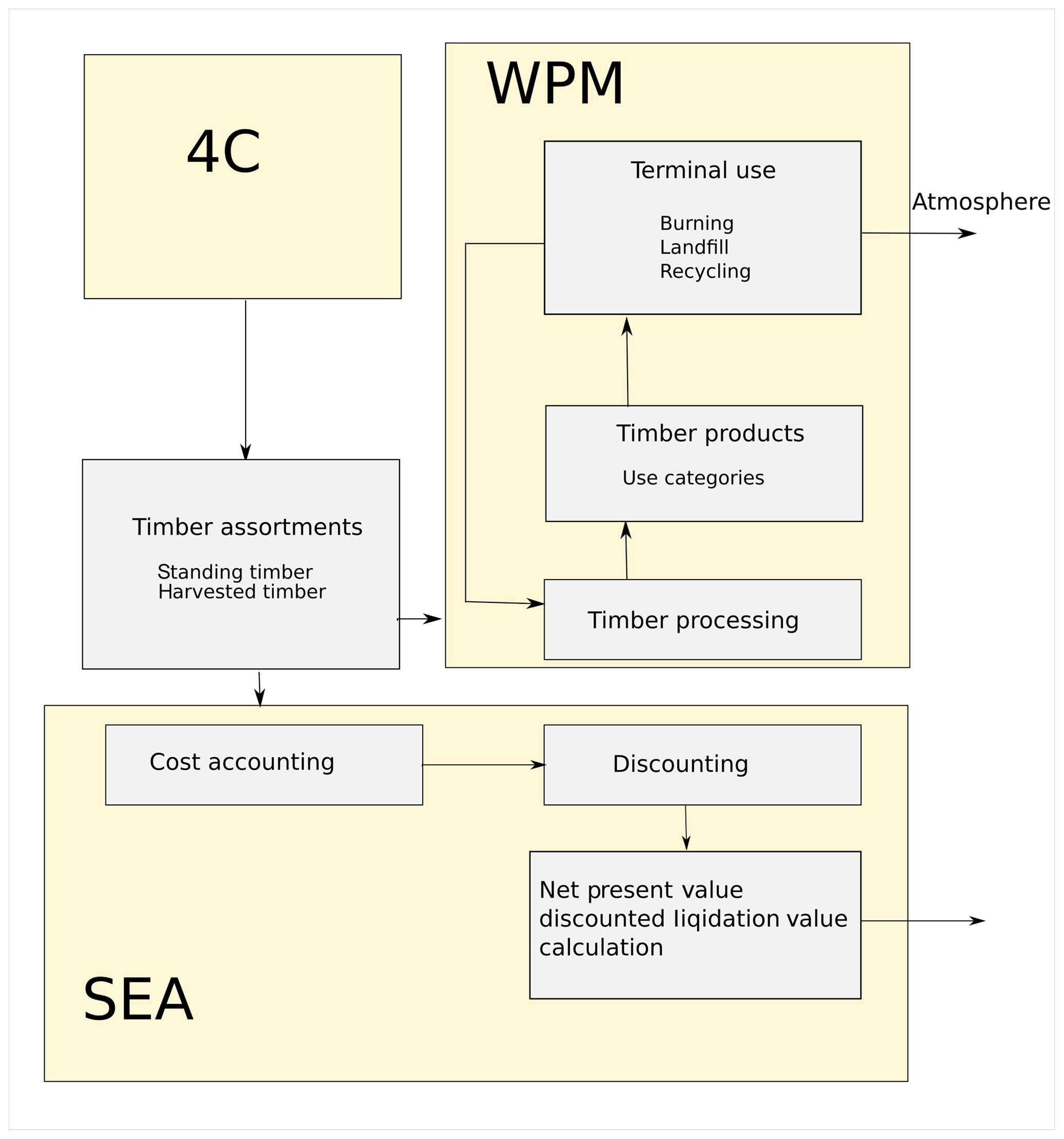
Wood product model and socio-economic analysis

A wood product model (WPM) is integrated in 4C. It is based on a concept introduced by Karjalainen et al. (1994) and further developed by Eggers (2002). The WPM simulates carbon pools and fluxes in the forest sector. The parameters are based on aggregated values of German timber market reports, available regional data, and parameters according to Eggers (2002). The WPM allows the grading of the harvested and standing timber, the processing of the timber, and allocation of timber to wood products, and it includes the retention period of timber in the final products and later on in landfills. Finally, a socio-economic analysis tool (SEA) (Fürstenau et al., 2007) calculates costs, revenues, and subsidies of forest management as well as the net present value (NPV) and liquidation value of the standing stock (Fig. 2); see Lasch-Born et al. (2018).

Figure 2 Model framework 4C (as presented in Fig. 1) coupled with the wood product model (WPM) and socio-economic analysis tool (SEA) (Eggers, 2002; Fürstenau et al., 2007).

Disturbances

The implementation of biotic disturbances follows a framework of modelling functional groups of biotic agents proposed by Dietze and Matthes (2014). In this framework, insects and pathogens are clustered upon their pathway of damaging the plant and abstracted on the level of functional groups (defoliators, xylem clogger, phloem feeder, root disturber, stem rot). In addition, we also implemented the growth and impacts of hemiparasitic European mistletoe (Viscum album L.) (Kollas et al., 2018). Currently, six pathways of damaging the plant have been implemented: (a) foliage loss, (b) reduction in water supply rate, (c) carbon loss, (d) fine root loss, (e) increase in tree mortality, and (f) combined increase in tree transpiration and carbon loss. The idea of this approach is to connect 4C with dynamic pest and pathogen models as well as disturbance scenarios. Information about the disturbance agent dynamics can stem from process-based models, empirical observations, or scenarios. Thus, disturbances have to be prescribed externally as an input time series, but their effects on the forest stand are modelled within 4C on a physiological basis. The prescription consists of the functional group of the disturbance, the disturbance year, and the damage level (e.g. defoliators imply reductions of foliage biomass between 0 % and 100 %), which then influences the affected processes within 4C.

If 4C is applied in the disturbance mode, an additional carbon pool is initialized, representing non-structural carbon stored in the tree (the so-called NSC pool). This pool is initialized during the tree initialization, and its maximum size depends on the carbon stored within the three biomass compartments sapwood, branch and twig wood, and coarse root wood (differentiated for coniferous and deciduous trees based on data reported by Hoch et al., 2003). By default, the simulation then starts with the NSC pool being completely filled. The surplus of carbon for allocation into damaged tissues is only available at the end of the disturbance year, while refilling of the NSC pool can continue for many years until the pool's maximum size is reached. For more details, see Lasch-Born et al. (2018).

2.1.4 Input data needs

The model requires daily meteorological data (temperature, precipitation, relative humidity, air pressure, wind velocity, and global radiation). Furthermore, annual CO₂ concentration and nitrogen deposition are necessary inputs.

Information about the forest can be provided at two levels of detail: at the stand level, average values of diameter at breast height (DBH), height, stem number or basal area, age, and species type are needed. From these data, single trees are generated using distribution functions. These functions were derived from Gerold (1990) and are based on Weibull distributions. They allow determining DBH values from the average DBH as long as the basal area is reached. The heights corresponding to the derived diameters are calculated with various diameter–height functions from the literature. The generated single trees are grouped into cohorts according to their DBH. The cohorts together represent the average stand values (see chapter 2.4 in Lasch-Born et al., 2018). At tree level, individual tree measurements (DBH, height, height of the crown base, species, and age) are needed and used to aggregate cohort data. Generally, individual tree data are better suited for initializing 4C because the cohorts can be estimated more realistically from individual tree data, but the stand-level initialization also yields realistic tree cohorts.

The description of the soil layers follows the soil horizons. At least the thickness and texture of the horizons are required as is their carbon and nitrogen content. Further important variables are pH, bulk density, pore volume, field capacity, and wilting point. If the last three entries are missing, they can also be estimated via pedotransfer functions from texture (Russ and Riek, 2011; Wösten et al., 2001).

2.2 Previous model evaluations and applications

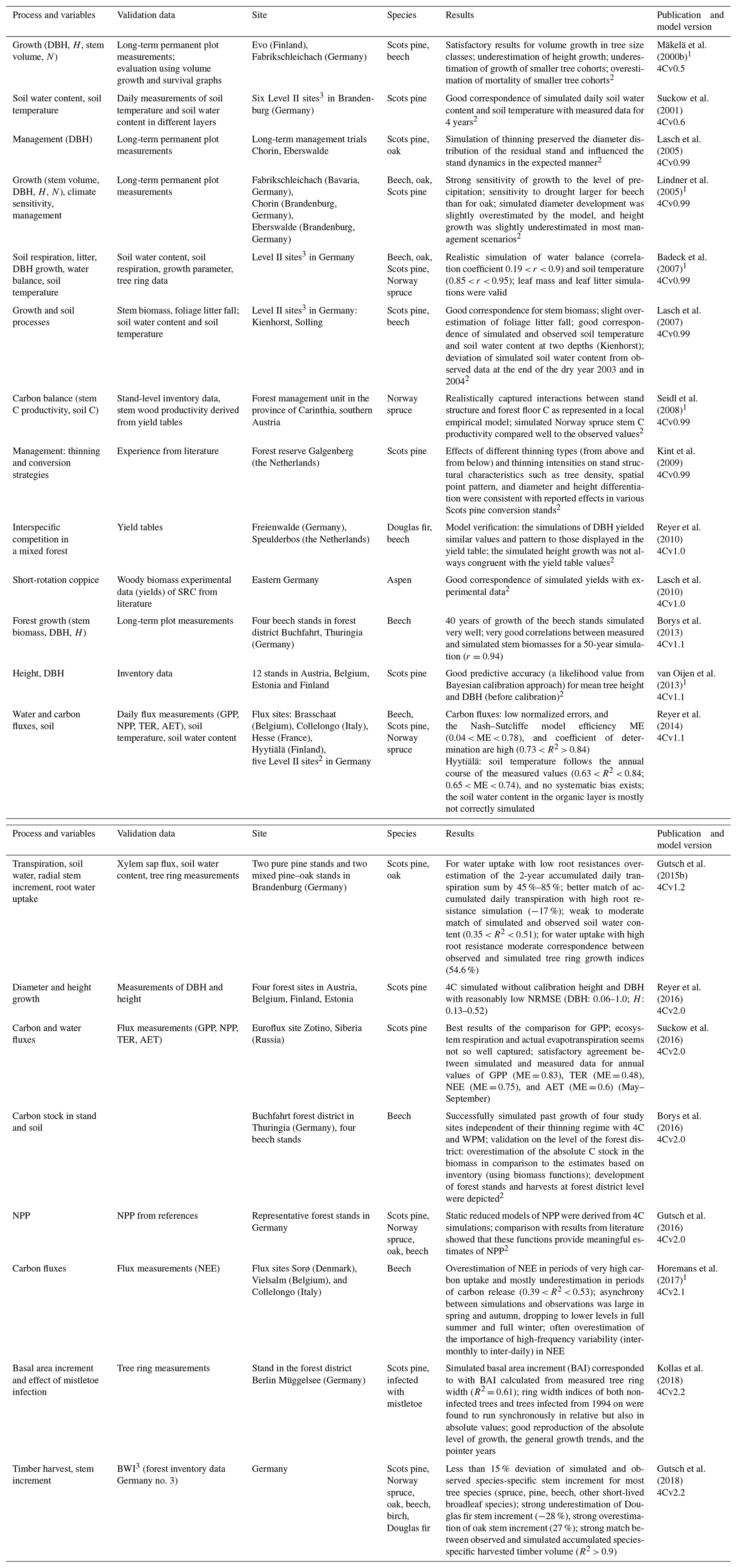
Table 1 Overview of studies in which different species, processes, and variables of 4C were evaluated (DBH – diameter at breast height, H – height, N – stem number, AET – actual evapotranspiration, NPP – net primary production, NEE – net ecosystem exchange, TER – total ecosystem respiration, GPP – gross primary production).

¹ Model comparisons.
² Only qualitative evaluation; no quantification of model–data mismatch available.
³ ICP Forests intensive monitoring plots.

Since the first applications of 4C, tests, evaluations, and model comparisons have been carried out for various forest stands and different processes within 4C (Table 1). The evaluations find 4C applicable to a wide range of environmental conditions and research questions but also highlight deficits. Using these previous evaluations in combination with the detailed results from the selected forest sites of this study, we will draw conclusions for further model development and improvement in the Discussion section.

The earlier applications of the model covered a wide range of research questions and issues. The most relevant objectives were (i) the carbon and water balance of forests under climate change, (ii) analysis of adaptive management under climate change, (iii) risks and benefits of climate change in forestry, (iv) energy potentials from forestry and short-rotation coppices, and (v) economic analysis of management units under climate change. A more detailed overview is given in the Supplement (Table S1 in the Supplement).

2.3 In which ways is 4C different from other forest models?

Medlyn et al. (2011) have developed a classification of models used to project climatic impacts on forest productivity which differentiates process-based stand models, terrestrial biogeochemical models, hybrid models, carbon-accounting models, gap models, and dynamic global vegetation models. This classification provides a starting point to explain the ways in which 4C is different from other forest models: in a narrow sense, 4C can be classified as a “process-based stand model” sharing key elements in terms of process description (see Sect. 2.1) with other models from that class such as GOTILWA+ (Keenan et al., 2012) and 3D-CMCC (Marconi et al., 2017). However, 4C also contains elements of “gap models” such as PICUS (Lexer and Hönninger, 2001) and FORCLIM (Bugmann, 1996), especially with regard to the canopy structure (see chapter 2.1. of the model description; Lasch-Born et al., 2018) and the inclusion of nutrient and water stress through production modifiers (see chapter 4.2. of the model description; Lasch-Born et al., 2018). Combining the strengths of different model types is a key feature of 4C, and while 4C represents forest complexity by incorporating the key processes of forest growth and dynamics in a mechanistic way, it is also simple enough to run without input data that are challenging to obtain for a larger number of forest stands such as detailed tree positions. Thus, it can be applied relatively easy to a larger number of forests stands as opposed to some of the other models in the same classes, and hence 4C can also potentially be applied at larger spatial scales such as regional or country level. Moreover, as opposed to other process-based stand models, 4C operates key physiological processes on daily to weekly timescales instead of sub-daily resolution and is thus computationally efficient enough to be applied over longer time frames and can cover many climate and management scenarios. Within the Intersectoral Impact Model Intercomparison Project (ISIMIP – https://www.isimip.org/, last access: 30 October 2020), 4C will be compared at the sites analysed here and further sites with other mechanistic climate-sensitive forest models. This will yield further insights about model structural uncertainties and how different models address these as well as how different the ensemble of forest models in Europe actually is.

2.4 Test sites, data, and simulation set-up

Table 2 Site and stand characteristics; data source: PROFOUND database (Alt. – altitude, T – annual temperature, P – annual precipitation sum, H – height, DBH – diameter at breast height).

^* Source: derived from Horemans et al. (2017).

To evaluate the current version of 4C regarding long-term growth as well as water and carbon fluxes, we selected four sites at Peitz (Germany), Solling (Germany), Sorø (Denmark), and Hyytiälä (Finland) representing the main central European tree species from the PROFOUND database to allow us to test forest models against a wide range of observational data (Reyer et al., 2020, 2019). Additional data sources (Tables 2 and S3 in the Supplement) for the sites were also used. For Peitz (Scots pine), Solling (Norway spruce), and Hyytiälä (Scots pine with some ingrowing Norway spruce) we evaluated forest growth by stem biomass (BM) and diameter at breast height (DBH) or geometric mean diameter (DG) measurements. These data were not available for Sorø from real measurements in sufficiently long time series. Furthermore, for Hyytiälä and Sorø (common beech) flux data were available. We did not recalibrate any parameters for the considered sites.

2.4.1 Climate, soil, stand, and observational data

Climate, stand, soil, and observational data for model evaluation were available from the PROFOUND database (Reyer et al., 2019) In addition to the gap-filled half-hourly flux data from the PROFOUND database we used the monthly and annually aggregated data from FLUXNET (http://fluxnet.fluxdata.org/data/fluxnet2015-dataset/, last access: 28 March 2017). We checked the half-hourly flux data and removed implausible data on a daily basis. Some additional data are used for the initialization of the soil profile for Hyytiälä, which are based on Haataja and Vesala (1997).

2.4.2 Management

All sites were simulated considering a management system which realizes stem removal according to the inventory records. Therefore, the time of occurrence and the intensity of thinnings have been prescribed for the respective runs. The type of thinning (e.g. thinning from above) was also selected on the basis of available management information. Peitz was managed with moderate thinning from below with a target stem number and 11 management interventions during the whole simulation period. Solling, Sorø, and Hyytiälä were managed with thinning from above with the target stem number and 13, 1, and 3 management interventions, respectively, during the simulation periods.

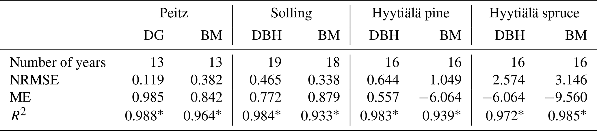
Table 3 Statistics for the three sites (DG – geometric mean diameter, DBH – diameter at breast height, BM – stem biomass, number – number of values).

^* p < 0.001

2.5 Evaluation metrics

To evaluate growth at Peitz, Solling, and Hyytiälä, we selected the variables arithmetic mean diameter at breast height (DBH) or the geometric mean diameter (DG) and stem biomass (BM), which were analysed at an annual time step. The choice of different diameter-based variables (DBH, DG) results from the data availability in the PROFOUND database. We applied regression analysis between observed and simulated values to determine the coefficient of determination R², its significance (with SigmaPlot for Windows Version 11.0), and the model efficiency ME (Loague and Green, 1991):

$$\begin{array}{}\text{(23)}& \text{ME}=\mathrm{1}-{\displaystyle \frac{\sum _{i=\mathrm{1}}^N(O_i-P_i{)}^{\mathrm{2}}}{\sum _{i=\mathrm{1}}^N(O_i-\stackrel{\mathrm{‾}}{O}{)}^{\mathrm{2}}}},\end{array}$$

where O_i represents observation values, P_i represents simulation values, $\stackrel{\mathrm{‾}}{O}$ is the mean of observation values, and N is the number of values. ME estimates the proportion of variance of the data explained by the 1:1 line and is an overall indication of the goodness of fit (Mayer and Butler, 1993); a positive value indicates that the simulated values describe the trend in the measured data better than the mean of the observations (Medlyn et al., 2005a; Smith et al., 1997). Furthermore, we calculated the normalized root mean square error NRMSE (Keenan et al., 2012):

$$\begin{array}{}\text{(24)}& \text{NRMSE}={\displaystyle \frac{\sqrt{\frac{\mathrm{1}}{N}\sum _{i=\mathrm{1}}^N(O_i-P_i{)}^{\mathrm{2}}}}{{\mathit{\sigma }}_{\text{obs}}}},\end{array}$$

where σ_obs represents the SD of the observation values.

Where available, we evaluated carbon (net ecosystem exchange, NEE; gross primary production, GPP) and water fluxes (actual evapotranspiration, AET), soil temperature (ST), and soil water content (SWC) in different layers using the same statistical measures on daily and monthly (and annual) timescales.

We also analysed the inter-monthly and inter-annual variability of the carbon and water fluxes. To this end we applied the method described by Keenan et al. (2012) and Vetter et al. (2008) to the monthly and annual time series of observed and simulated GPP, NEE, and AET. The inter-monthly variability (IMV) is calculated as follows.

$$\begin{array}{}\text{(25)}& {\text{IMV}}_{m,t}^V=V_{m,t}-{\stackrel{\mathrm{‾}}{V}}_m\end{array}$$

${\stackrel{\mathrm{‾}}{V}}_{m,t}$ is the monthly variable (GPP; NEE, AET) (sum) of month m and year t, and ${\stackrel{\mathrm{‾}}{V}}_m$ is the long-term monthly mean of the variable V for month m (m=1, 12).

The inter-annual variability (IAV) is calculated for the annual time series of the considered variables V.

$$\begin{array}{}\text{(26)}& {\text{IAV}}_t^V=V_t-\stackrel{\mathrm{‾}}{V}\end{array}$$

V_t is the annual V of year t, and $\stackrel{\mathrm{‾}}{V}$ is the long-term mean of V.

The resulting monthly and annual “normalized” times series (observed and simulated) were compared and subjected to statistical and graphical analyses.

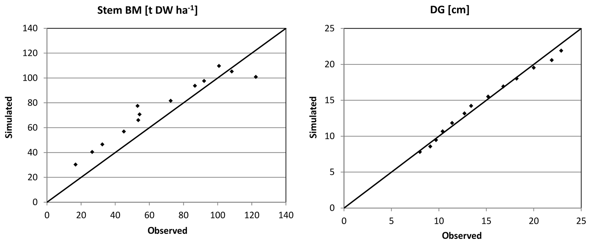
Figure 3 Simulated (sim) vs. observed (obs) DG and stem biomass (BM) for Peitz in the form of scatter plots with a 1:1 line.

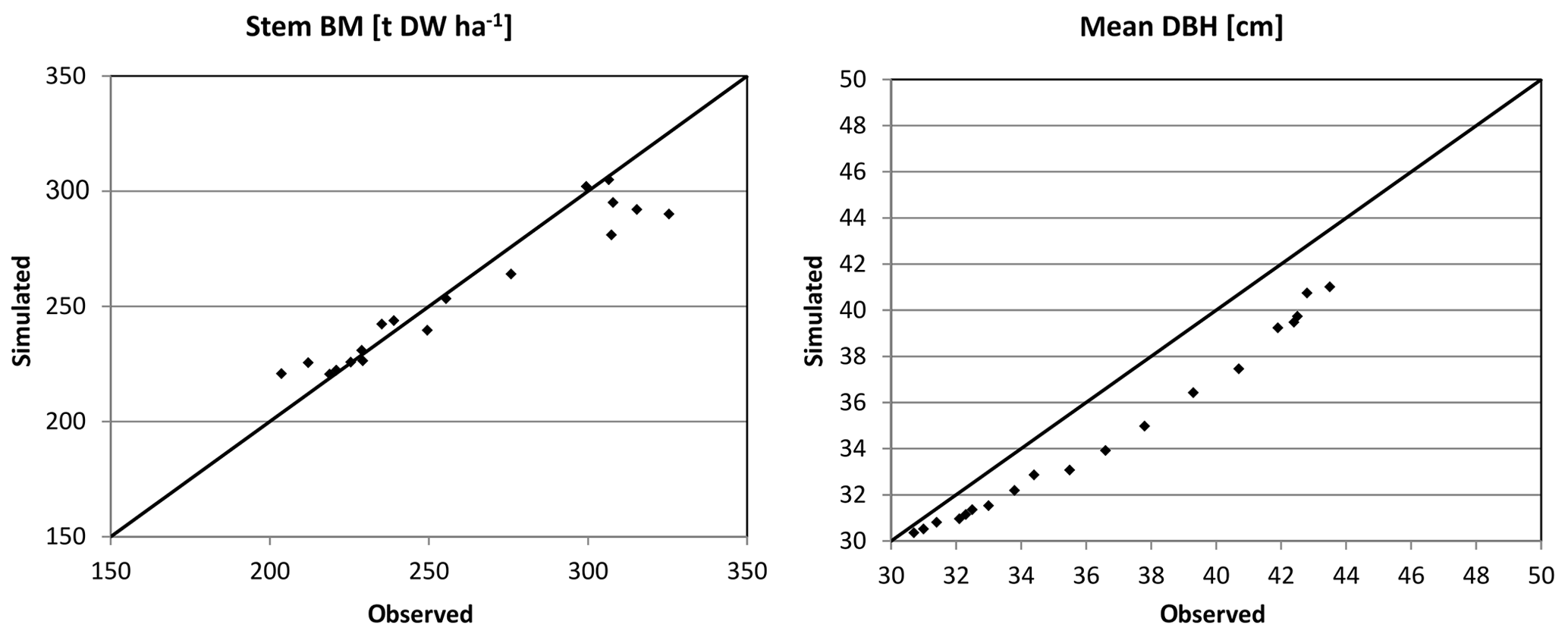
Figure 4 Simulated (sim) vs. observed (obs) DBH and stem biomass (BM) for Solling in the form of scatter plots with a 1:1 line.

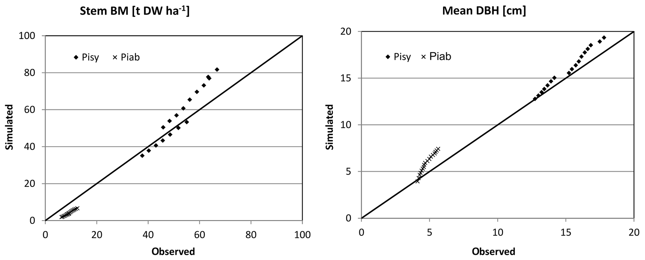
Figure 5 Simulated (sim) vs. observed (obs) DBH and stem biomass (BM) for Hyytiälä (Pisy – pine, Piab – spruce) in the form of scatter plots with a 1:1 line.

3 Results

3.1 Forest growth

Based on the statistical measures, 4C shows the best performance in terms of ME of DG and BM for Peitz. For Solling the model performance is slightly lower than for Peitz, but ME is still well above 0.7 (Table 3). For Hyytiälä, the model performance for DBH of pine (ME = 0.557) is better than for spruce (ME = −6.06); however, the performance measures for the stem biomass are low. Negative values of ME indicate that the residual variance (observed minus simulated) is greater than the variance of the observed values. For Hyytiälä, 4C overestimated DBH for both pine and spruce, overestimated stem biomass for pine (ME = −6.06), and underestimated stem biomass for spruce (ME = −9.56) (Figs. 5 and S3 in the Supplement).

NRMSE and ME show better results for DBH and DG than for stem biomass for Peitz and Hyytiälä (Table 3). The stem biomass simulations are less precise for all sites because biomass simulation depends on simulated height increment and NPP allocation to sapwood as well as the sapwood senescence rate. The large negative ME values for DBH (−6.064) and BM (−9.56) of spruce in Hyytiälä indicate a poor performance of the model. 4C underestimated the BM and overestimated DBH of spruce in this forest (Figs. 5 and S3). The values of R² are very high for all variables (0.933 < R² < 0.988) and sites but are of limited value since they do not provide a comprehensive measure of model performance (Medlyn et al., 2005b).

Table 4 Annual long-term means (± SD) of water and carbon fluxes in Sorø (1997–2012) and Hyytiälä (1996–2014).

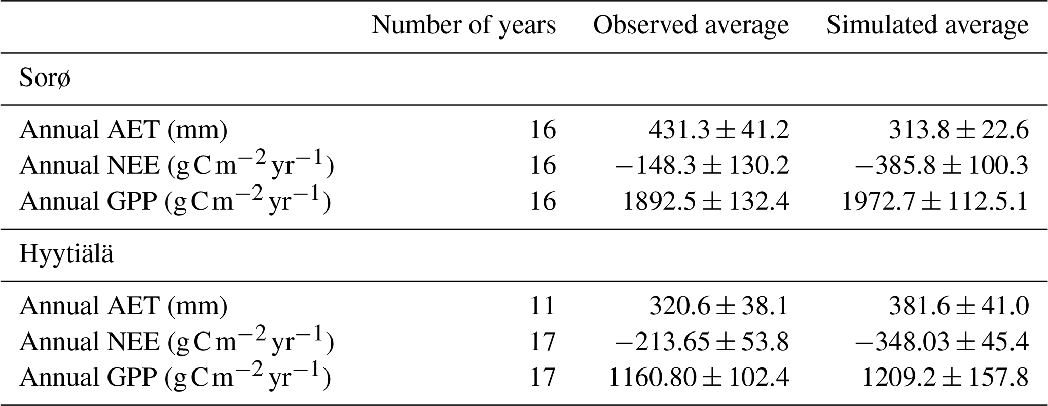
Table 5 Evaluation metrics for daily, monthly, and annual sums of AET, NEE, and GPP for Sorø (1996–2012) and Hyytiälä (1996–2014).

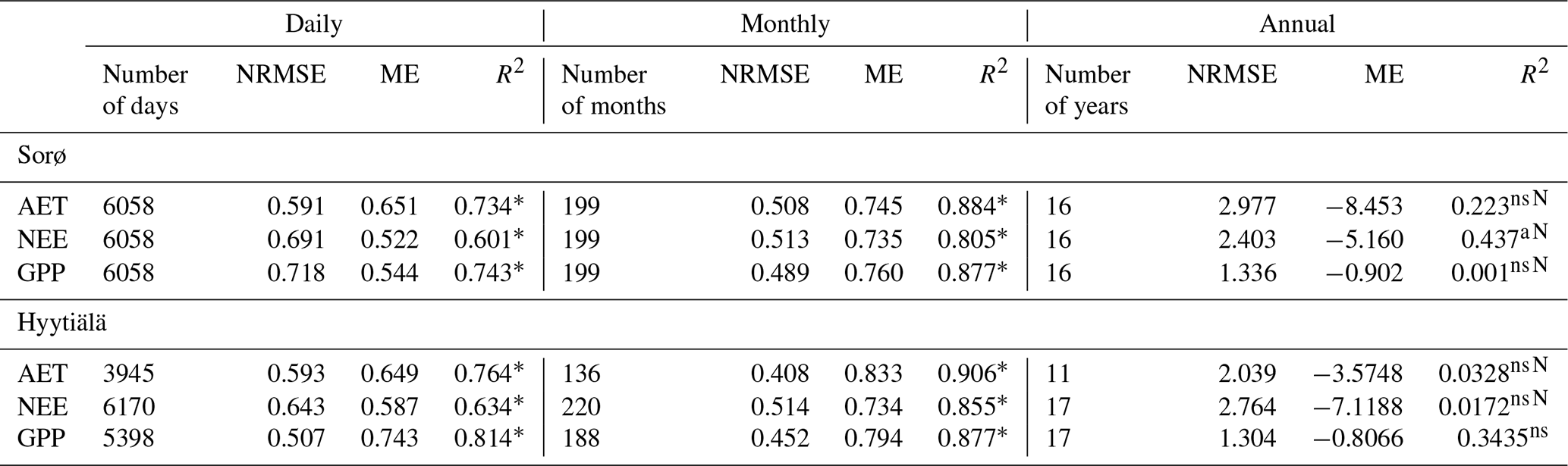
^* p < 0.001; ^ns not significant; ^N normal distribution.

3.2 Carbon and water fluxes

3.2.1 Evaluation over long timescales at different time resolutions

The averages of the simulated annual fluxes in comparison with the observed averages show good correspondence for GPP for Sorø and Hyytiälä (Table 4). In Sorø, 4C overestimates the long-term average GPP by 3.7 % and in Hyytiälä by 3.5 % (Table 4). NEE is clearly underestimated in Sorø ($-\mathrm{148.3}\pm \mathrm{130.2}$ $\mathrm{g}\mathrm{C}{\mathrm{m}}^{-\mathrm{2}}{\mathrm{yr}}^{-\mathrm{1}}$ observed, $-\mathrm{385.8}\pm \mathrm{100.3}$ $\mathrm{g}\mathrm{C}{\mathrm{m}}^{-\mathrm{2}}{\mathrm{yr}}^{-\mathrm{1}}$ simulated) and Hyytiälä ($-\mathrm{213.65}\pm \mathrm{53.8}$ $\mathrm{g}\mathrm{C}{\mathrm{m}}^{-\mathrm{2}}{\mathrm{yr}}^{-\mathrm{1}}$ observed, $-\mathrm{348.03}\pm \mathrm{45.4}$ $\mathrm{g}\mathrm{C}{\mathrm{m}}^{-\mathrm{2}}{\mathrm{yr}}^{-\mathrm{1}}$ simulated) on long-term average. The same is true for the AET in Sorø (431.3±41.2 mm observed, 313.8±22.6 mm simulated), but it is slightly overestimated for Hyytiälä (320.6±38.0 mm observed, 381.6±41.0 mm simulated). The R² (Sorø: $\mathrm{0.0001}<R^{\mathrm{2}}<\mathrm{0.437}$, Hyytiälä: $-\mathrm{7.1188}<R^{\mathrm{2}}<-\mathrm{0.8066}$) and ME (Sorø: $-\mathrm{8.453}<\text{ME}<-\mathrm{0.902}$, Hyytiälä: $\mathrm{0.0172}<\text{ME}<\mathrm{0.3435}$) indicate very low correspondence between observed and simulated annual values (Table 5).

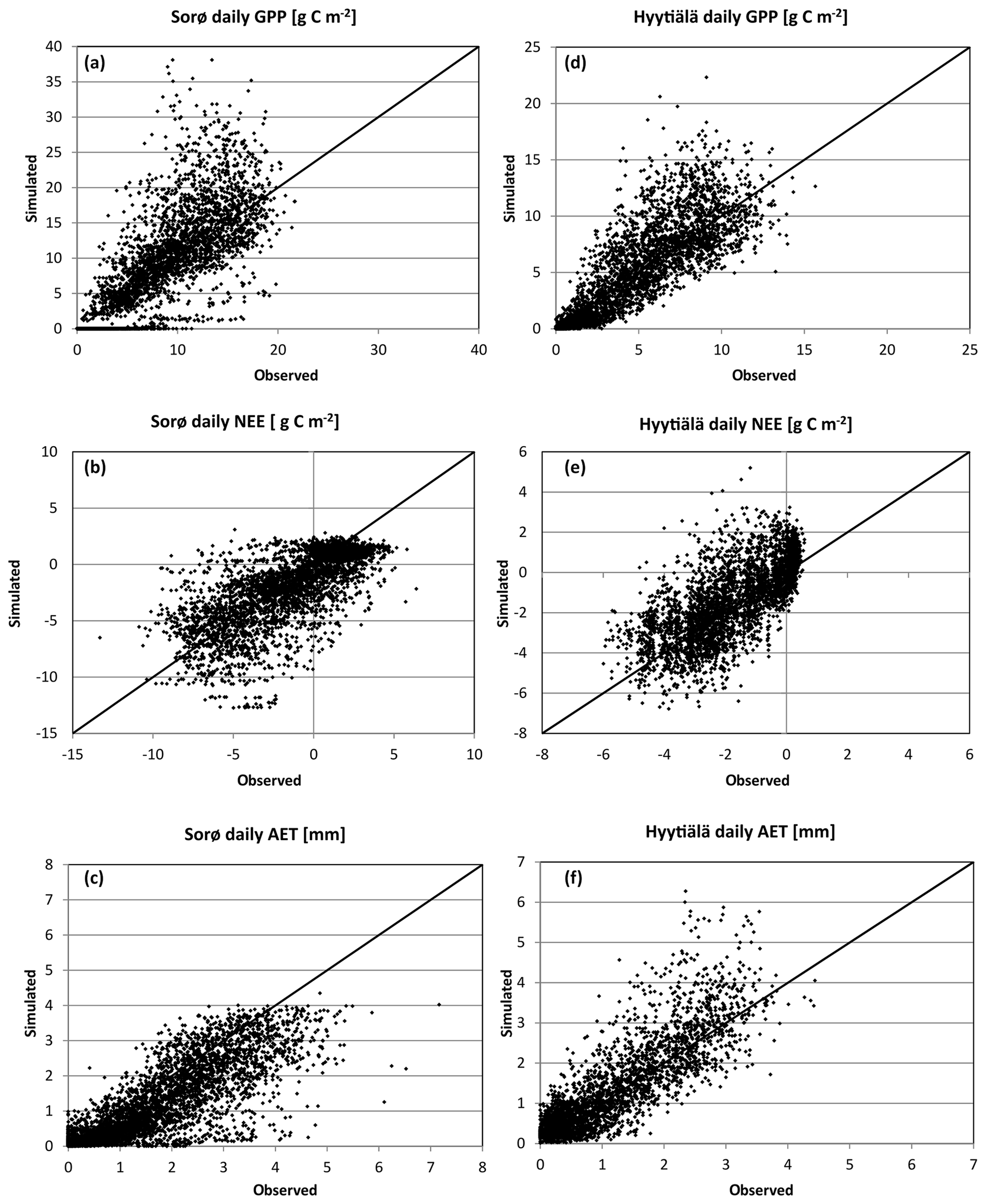
Figure 6 Simulated vs. observed daily GPP, NEE, and AET in Sorø (a–c) and Hyytiälä (d–f). The black line shows a 1:1 relationship.

For daily and monthly sums of fluxes, the evaluation metrics indicate much higher agreement between simulated and observed values, and the monthly results show even better agreement with observations than the daily results (Table 5). The evaluation metrics for Hyytiälä are slightly better than for Sorø, especially for AET (e.g. Hyytiälä: R² = 0.764, Sorø: R² = 0.734 for daily values) and GPP (Hyytiälä: R² = 0.814, Sorø: R² = 0.743 for daily values). For Sorø, 4C simulates days without any GPP, while GPP values greater than zero were observed. Daily AET is underestimated for days with a high observed AET (greater than 4 mm). For Hyytiälä, 4C clearly overestimates GPP and AET but also NEE for single days by more than 50 % (Fig. 6d–f). The intra-annual variability on a monthly scale in Sorø for the three variables (Fig. 6a–c) shows that 4C underestimates GPP from January to April, but during the vegetation period the GPP is clearly overestimated (and NEE underestimated). AET is underestimated throughout the year. In Hyytiälä, 4C overestimates the monthly GPP and underestimates the NEE during the vegetation period from May until July (Fig. S11 in the Supplement). The variability of the monthly GPP from May until August is higher for the simulated values than for the observed values in Sorø (Fig. S7 in the Supplement); for Hyytiälä, it is the other way around. The monthly AET is overestimated throughout the year in Hyytiälä.

3.2.2 Inter-monthly (IMV) and inter-annual variability (IAV)

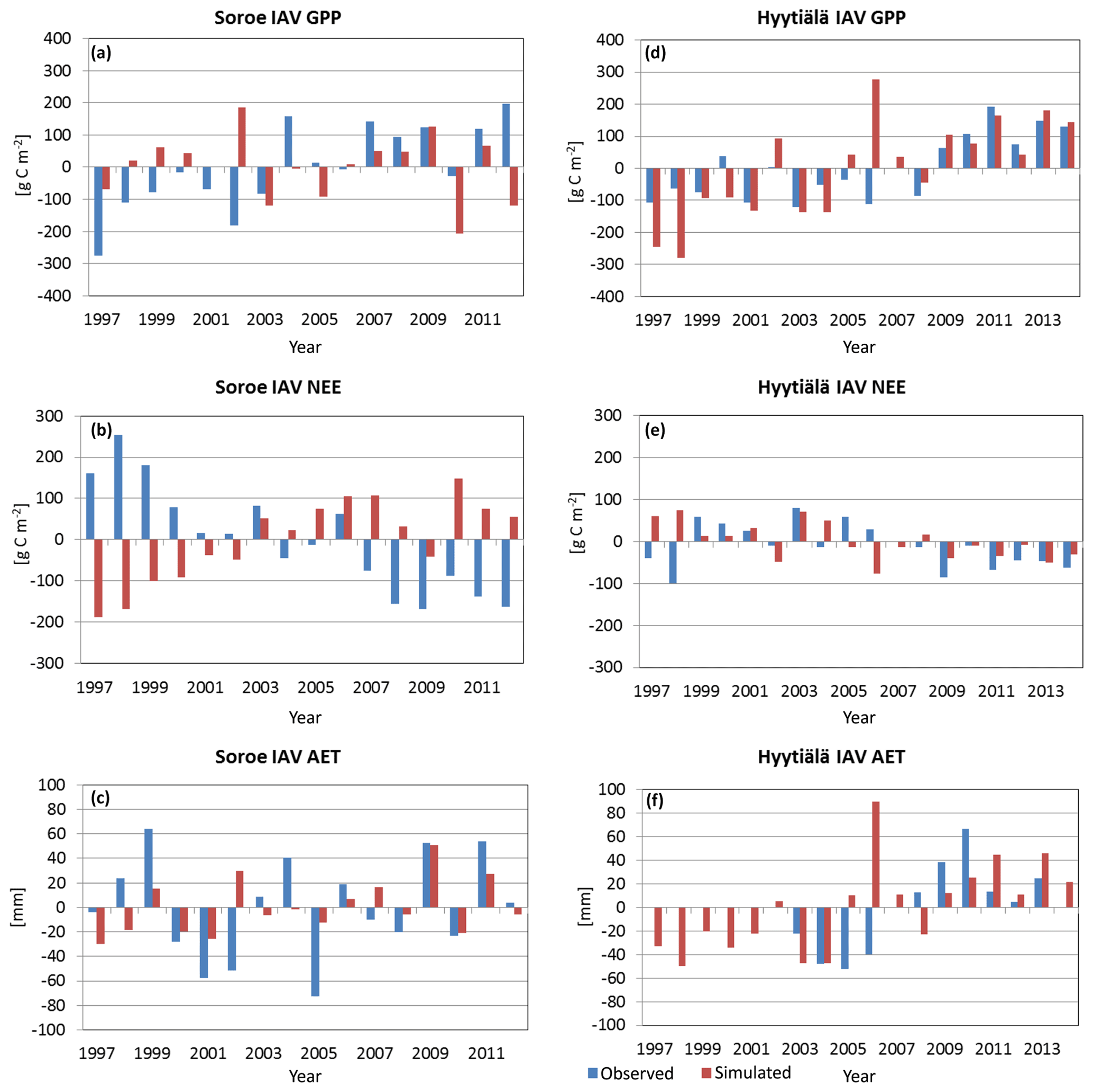
Figure 7 Inter-annual variability (IAV) of GPP, NEE, and AET (sim – simulated and obs – observed) in Sorø (a–c) and Hyytiälä (d–f).

The simulated and observed inter-annual variability is nearly the same order of magnitude for both sites and for the three variables except for a few years for Sorø (1997: GPP, NEE) and Hyytiälä (1997/98, GPP; 2006, AET) (Fig. 7). The signs of IAV were best captured for Hyytiälä with 82 % for GPP, 65 % for NEE, and 70 % of the years for AET. In Sorø, the signs of IAV of GPP and NEE are not captured by the model; in most of the years the signs are opposite to observed IAV except for AET (63 %).

Figure 8 Distribution of the magnitude for the inter-monthly variability values (IMV) of observed (obs, in upper part of the graphic) and simulated (sim, in the lower part of the graphic) monthly sums of GPP, NEE, and AET in Sorø (a–c) and Hyytiälä (d–f). The graphs show the median, the 25th and 75th percentile (box), the 10th and 90th percentile (whiskers), and outliers (black dots).

The analysis of inter-monthly variability with the normalized IMV data shows similar interquartile ranges for simulated and observed IMV but a clearly higher range of the IMV of simulated GPP and NEE for Sorø (Fig. 8a–c). The IMV of AET differs in the interquartile ranges for simulated and observed data, but the range is similar. The simulated variables for Hyytiälä show a lower variability, especially for the NEE, and also somewhat lower for the AET. The simulated GPP has a smaller range of inter-monthly variability than the observed GPP (Fig. 8d–f).

3.3 Soil temperature and water content

Figure 9 Time series of observed and simulated daily soil temperature at 5 cm of depth (a) and time series of observed and simulated daily soil water content at 8 cm of depth (b) in Sorø for the period 1996–2012.

Table 6 Daily and monthly statistics of soil temperature (ST) and soil moisture (SWC) for Sorø 1996–2012 and Hyytiälä (1996–2014).

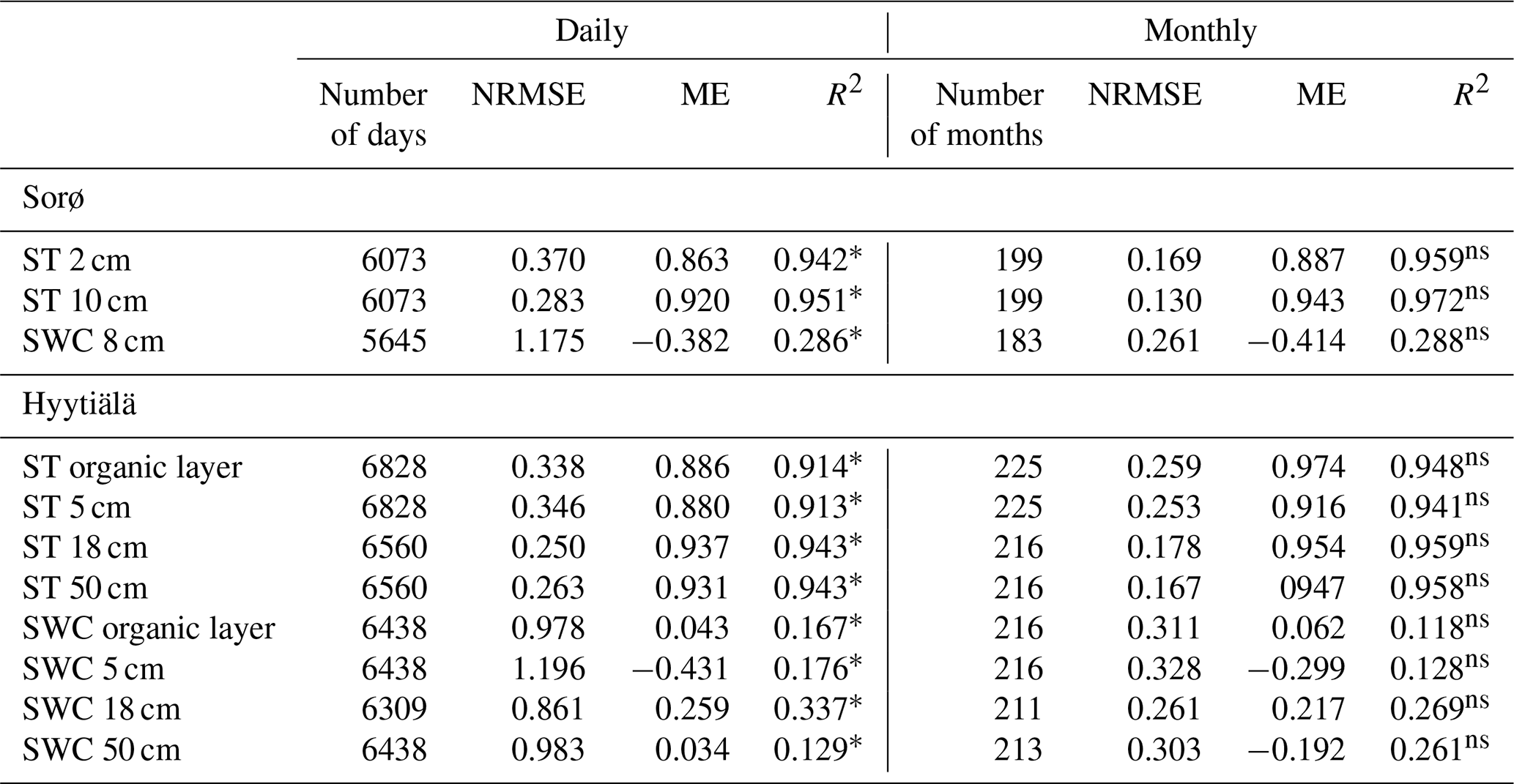
^* p < 0.001; ^ns not significant.

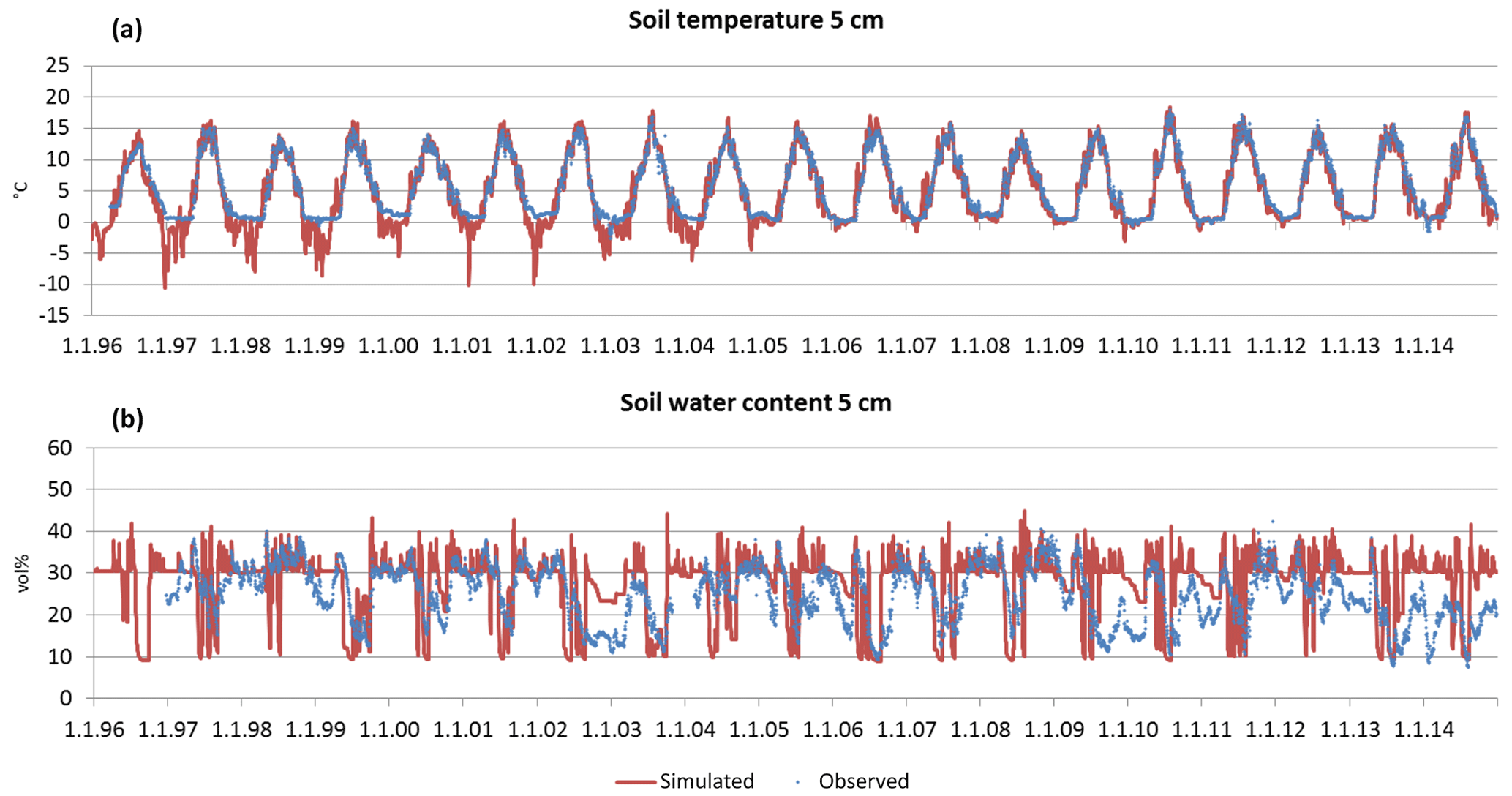
Figure 10 Time series of observed and simulated daily soil temperature (a) and time series of observed and simulated daily soil water content (b) at 5 cm of depth in Hyytiälä for the period 1996–2014.

The simulated soil temperature (ST) fits very well with the observed data in Sorø (Fig. 9a) and Hyytiälä (Fig. 10a) (0.887 < ME < 0.974). With increasing soil depth, the bias between simulated and observed values decreases, which is reflected in a decreasing NRMSE and an increasing ME and R² (Table 6). This applies for the daily and monthly statistics, with the statistics on a monthly level being slightly better than on a daily level in most cases. In Hyytiälä, the simulated soil temperature in winter is lower than the observed temperature for the years 1996 until 2005, and consequently the simulated depth of frost is also lower (Fig. 10a; for more details see Fig. S15 in the Supplement).

In contrast, the simulations of soil water content (SWC) are less accurate for both sites. Comparing simulated and observed soil water content for all soil layers leads to very low R² values (monthly: 0.118  < R² < 0.288, daily: 0.167 < R² < 0.337) and also to low ME (Table 6). In Sorø, the model underestimates the water content in the upper mineral layer, especially in wintertime (Fig. 9b). During summer, the model simulates an exhaustion of the soil water content up to the wilting point for several days and more often than observed. Altogether, the model responds to precipitation faster than is indicated by the measurements.

For Hyytiälä, the results are similar (Fig. 10b). The visual inspection for two layers shows a similar picture as in Sorø: an underestimation during wintertime and a more frequent exhaustion of the soil water during summer. The observed water uptake frequently reaches a depth of 50 cm, while the simulated water uptake only reaches a maximum depth of 50 cm in the very dry months of July and August 2006 (Fig. S16 in the Supplement), with only one-third and half of the precipitation sum of the long-term mean, respectively. The interquartile ranges and the ranges of outliers of soil water content are mostly higher for the simulated than for the measured values (Fig. S12, right, in the Supplement).

4 Discussion

In this paper, we have analysed the capability of 4C to reproduce forest growth, carbon, and water fluxes at different temporal resolution as well as soil water content and soil temperature in different soil layers for four forest stands in temperate and boreal regions of Europe. As is often the case when evaluating complex forest models, not all sites and scales can be evaluated in the same way due to different data availabilities. Nevertheless, we present a very comprehensive evaluation of the model which provides important information on the applicability of 4C. In the following, we discuss the evaluation results and provide future scientific users of the model with recommendations on how to best use the model in specific cases and an impression of the reliability of the model results regarding various research questions.

4.1 Evaluation of forest growth

Overall, the ability of 4C to reproduce the dynamics of forest growth clearly differs from site to site. Therefore, we recommend that model users thoroughly evaluate the model before any application. 4C performs best for the monospecific coniferous stands at Solling and Peitz independent of the evaluation metrics. In particular for Peitz, which features the longest observational time series of Scots pine growth, we observe the best agreement between the model and data (Figs. 3 and S1 in the Supplement). For Solling, 4C underestimates the development of DBH (Figs. 4 and S2 in the Supplement). Ibrom (2001) and Ellenberg et al. (1991) found similar carbon storage in this spruce stand in 1967 of 9314 g C m⁻² as initialized by 4C based on tree dimensions (10 840 g C m⁻²), indicating that basic assumptions about stem form and wood density are appropriate. Our initialization prescribes the same number of trees (595 ha⁻¹) as observed but strongly underestimates foliage (needle) mass (4C: 422.5 vs. 868 g C m⁻² found by Ellenberg et al., 1991). We applied the fixed parameter η_s (foliage to sapwood area relationship) to estimate foliage mass, which could lead to this underestimation. Furthermore, the estimation of sapwood area from DBH used for initialization is also uncertain. Consequently, our initialization leads to a smaller leaf area index (LAI) of 5.1 m² m⁻² in 1990 compared to a value of 7 m² m⁻² reported by Ibrom (2001) for the same year. In 4C, the initialization of the foliage biomass and fine root biomass is estimated via a function depending on sapwood area and a parameter describing the foliage to sapwood area relationship. Therefore, it is possible that 4C's underestimation of DBH growth is due to the underestimation of foliage biomass during initialization. While foliage is underestimated, the initialization works well for DBH. Ibrom (2001) gives the values for mean DBH (35 cm) and mean top height (28 m), which are nearly matched by 4C with a DBH of 35 cm and mean top height of 31.8 m. The initialization of the height of tree cohorts uses height–diameter relationships from various yield tables, which can lead to deviations in comparison with measured data. We therefore recommend that model users check whether the foliage masses and height–diameter relationships found after initializing the model are comparable to locally and regionally derived relationships.

The quality of growth simulation in Hyytiälä differs for the two species. For Norway spruce, which is present in the understorey of this pine-dominated stand, stem biomass initialization is underestimated but growth is realistic, whereas the stem biomass growth of pine is slightly overestimated (Figs. 5 and S3). Because thinning is driven by observed stem numbers, stem biomass is overestimated after thinning because other trees were harvested in the model than in the real stand. Comparing simulated biomass data of stem biomass for the mixed stand at Hyytiälä with measurements (Fredrik Lagergren, personal communication, 2012) for the initialization year 1995, we find that pine stem biomass is in accordance with measurements, while spruce stem biomass is clearly underestimated (see Figs. 5 and S3). Therefore, we recommend that model users always check whether the trees removed in 4C during management are somewhat comparable in terms of size, for example, to those removed in reality if such data are available.

Earlier model evaluations of stand dynamics for different species such as pine, spruce, and beech in Germany by Lasch et al. (2005, 2007) and Lindner et al. (2005) demonstrated a sufficient ability of the model to reproduce forest growth in terms of DBH, height, and biomass. Thus, while in general we have confidence in the ability of 4C to simulate forest growth, it is important to keep in mind that 4C works with a site-independent species parameter set and we did not recalibrate any of the parameters locally. Thus, matching the absolute observed values could differ between Scots pine stands in Germany and Finland because of the uncertainty associated with fixed generic parameters (Collalti et al., 2016). For example, trees in Finland often develop crown shapes that are more adapted to reducing snow damage – this is an example for an adaptive trait that is evolutionary and is not considered in the model. Even though it is not necessary to recalibrate 4C before moving to a new site, we recommend that model users check whether data relating to the main model parameters have been collected and can be used to explain model–data mismatches.

4.2 Evaluation of carbon and water fluxes

We analysed the model's performance in simulating carbon and water fluxes using statistical measures on different timescales. For Sorø and Hyytiälä, 4C performed best when comparing simulation results with observational data on daily and monthly scales for GPP, NEE, and AET (Table 5). The main reason here is the strong dependence of daily and monthly water and carbon fluxes on the daily and seasonal course of temperature and radiation. This clear pattern disappears on the annual scale, and small deviations at the daily scale accumulate at the annual scale. Therefore, the relative importance of other variables besides the meteorological parameters, such as leaf area dynamics, transpiration limitation due to water shortage, the length of the growing season, and the ground vegetation, increases at the annual scale, thus rendering these simulation results more uncertain. Collalti et al. (2016) also found a better performance on a monthly scale than on an annual scale for both sites for their 3D-CMCC-FEM from the same model family. We therefore recommend that model users evaluate the model across different temporal scales to understand at what temporal scale confidence in the model results is adequate.

For both sites, 4C overestimated GPP and underestimated NEE on long-term average. This could be caused by the simplified simulation of ecosystem respiration in 4C (see Sect. 2.1.3). Because organ-specific dynamic respiration rates are hard to parameterize due to a lack of data, the respiration rate in 4C is a fixed fraction of GPP following an approach of Landsberg and Waring (1997). The SDs of the annual GPP are of similar magnitude for observations and simulation data, which indicates high variability from year to year in both datasets. For Sorø, the SDs of NEE are also very high for simulated (130 $\mathrm{g}\mathrm{C}{\mathrm{m}}^{-\mathrm{2}}{\mathrm{yr}}^{-\mathrm{1}}$) and (100 $\mathrm{g}\mathrm{C}{\mathrm{m}}^{-\mathrm{2}}{\mathrm{yr}}^{-\mathrm{1}}$) observed annual values, whereas for Hyytiälä the SDs are of a lower order of magnitude (54 and 45 $\mathrm{g}\mathrm{C}{\mathrm{m}}^{-\mathrm{2}}{\mathrm{yr}}^{-\mathrm{1}}$). In former model validation experiments with 4C for the site at Hyytiälä (Reyer et al., 2014), we concluded that systematic underestimation of NEE at low temperatures causes this deviation between measured and observed fluxes, which is still a problem. We therefore recommend that model users critically evaluate the role of respiration and carbon balances in their applications to ensure the model limitations are clearly spelled out when explaining the model results.

The annual course of GPP and NEE in Sorø shows a sharp increase in GPP with the start of the vegetation period (bud burst) which is faster than the simulated flushing. The phenological model of 4C (Schaber and Badeck, 2003; Schaber, 2002) for beech was derived from long-term observational data in Germany, and hence the model parameters might not represent the phenology of beech in Denmark. In fact, the average day of bud break for 1999–2009 in 4C is the day of the year 120, while Pilegaard et al. (2011) found values between 118 and 134, with a mean of 129. Furthermore, we did not consider ground vegetation because the ground vegetation implemented in 4C is not suitable for beech stands (see Sect. 2.1.2). Therefore, the simulated GPP is underestimated during the early springtime (Fig. S7). For Sorø, Horemans et al. (2017) discussed in great detail the differences between simulated and observed NEE for 4C and concluded that 4C overestimates the importance of high-frequency variability because 4C uses the daily temperature to redistribute the weekly calculated NEE, and the applied dependency is possibly too sensitive. Therefore, we recommend that model users assess the role of phenological changes and high-frequency variability in their study and, if that amount of detail is required, adjust the phenological parameters to local conditions.

4C simulates acceptable AET values on daily and monthly timescales (ME ≥ 0.65) but not on the annual scale. For Hyytiälä the statistics do not show a systematic bias of observed and simulated AET at daily and monthly timescale as for Sorø, where the long-term annual amount and the daily AET values are underestimated (Fig. 6, Table 6). The annual course of AET for Sorø as well as the normalized deviation between simulated and observed values show a large underestimation of AET during the vegetation period, in particular in the months prior to bud break (February to May) (Figs. S7 and S13 in the Supplement). In contrast, the simulated AET at Hyytiälä does not show such a strong bias (Figs. S11 and S14 in the Supplement). Like for GPP and NEE, the strong systematic bias at the Sorø site is a result of neglecting the observed ground vegetation in 4C. In the model we assume that there is no transpiration when there are no leaves. But in Sorø ground vegetation consisting of Anemone nemorosa L. and Mercurialis perennis L. exists before bud break (Pilegaard et al., 2001), and in that time the AET is clearly underestimated by the model. Based on reported transpiration values for the ground vegetation comparable to our pine sites at Hyytiäla (56 to 76 mm yr⁻¹; Launiainen, 2011) and Peitz (173 to 185 mm yr⁻¹; Lüttschwager et al., 1999), the ground vegetation in a beech stand at Sorø also explains the simulated deviation of 10 to 20 mm month⁻¹ from February to May (Fig. S11). High values of observed AET of more than 4 mm d⁻¹ show almost no correlation with radiation and only weak correlation with air temperature, but the approach of Penman–Monteith used in 4C calculates the potential evapotranspiration as a function of radiation and air temperature. Obviously, there are other factors that influence the AET. Furthermore, the soil data for field capacity, wilting point, pore volume, and percolation were only estimated by pedotransfer functions. This estimation might explain the underestimation of water supply causing the deviations in AET simulations from observations during the vegetation period of the trees. Unfortunately, in Sorø only the water content at 8 cm of soil depth is available. Here we could not perform a simulation run with measured soil water content values as model input to further disentangle probable reasons for the deviations in AET. For Hyytiälä these data were available from measurements, leading to a better simulation of AET, but here the simulation run with measured soil water content values as model input also does not change model outputs regarding AET, GPP, and NEE compared to the original simulated outputs. So, this model exercise also did not yield any further results other than the fact that the soil water does not play a role for the deviations from the measured AET at Hyytiälä for all timescales. We recommend that model users, similar to the evaluation of carbon fluxes, evaluate the model across different temporal scales and assess the role of ground vegetation for each stand.

Model validation with eddy covariance data is known to suffer from inherent problems (Medlyn et al., 2005b; Robinson et al., 2005). Therefore, we performed an informal interpretation of residual diagrams (Figs. S4 and S8 in the Supplement), showing positive correlations between the simulated values and the residual deviation for all variables (GPP, NEE, AET). This reveals a bias towards overestimation at high values simulated by the model at both sites. But since the model efficiency of greater than 0.5 of the daily and monthly values was sufficiently good (Table 5), we also analysed the inter-annual variability (IAV) with so-called normalized time series, indicating the variation from year to year between the observed and simulated annual values of GPP, NEE, and AET. At both sites the magnitude of inter-annual variability is similar between observations and simulations for all variables except for some years (Fig. 7). Yet, the signs of the IAV clearly differed more often for Sorø than for Hyytiälä. Furthermore, there is a strong trend in Sorø's simulated GPP and NEE opposite to the observed trends. 4C reproduced IAV of GPP, NEE, and AET clearly better for Hyytiälä than for Sorø. As a positive aspect with regard to climate sensitivity we note that for both sites the signs of simulated and for observed GPP IAV are negative in the extremely dry year 2003 (Granier et al., 2007), which provides some confidence that 4C is capturing such extreme conditions as were prevalent in 2003. The lower performance in Sorø can be explained by the imprecise simulation of evapotranspiration and available water in Sorø, which, in turn, influences the NEE through water limitations. It also underlines a problem in simulating the beech stand because of missing ground vegetation and imprecise timing of bud burst and leaf unfolding. Keenan et al. (2012) pointed out that terrestrial biosphere models often fail to explain the observed inter-annual variability in deciduous canopy phenology, which is key to matching the IAV of carbon and water fluxes in these kinds of forests. The IAV of the observations is caused by a high number of physical, biological, and anthropogenic factors affecting the photosynthesis, respiration, and water fluxes of forest ecosystems (Lagergren et al., 2008). The reproduction of the IAV by the model requires information about these factors and model approaches describing these known but often not measured factors. Overall, our results are in accordance with the finding of Baldocchi et al. (2018), showing from analysis of flux data a clearly higher IAV of NEE in a temperate deciduous forest than in a boreal evergreen forest. They explained the variability in ecosystem photosynthesis as the dominant factor causing IAV in NEE, which is confirmed by our results.

The fact that the AET in Sorø cannot be adequately modelled with 4C is also expressed by the inter-monthly variability, which is simulated lower than measured. For Hyytiälä, the interquartile ranges of observed IMV are larger not only for AET but also for NEE in comparison to simulated IMV. The latter could be caused by the imprecise simulation of ecosystem respiration (soil and stand). The IMV of monthly simulated NEE is clearly lower than the IMV of the observed NEE (Fig. 8) during the vegetation period. In Sorø, it is the other way around (see Fig. 8). GPP shows the same pattern. We suspect that this behaviour could be caused by differences in the length of vegetation period between coniferous and deciduous species as well as different climatic conditions. We recommend that model users analyse IAV and IMV for studies focusing on carbon exchange, which helps to detect reasons for low model efficiency at the annual timescale.

4.3 Evaluation of soil water content and soil temperature

Our results show that 4C is able to reproduce soil temperature at different depths in Sorø and Hyytiälä with good accuracy (all ME > 0.8) (Figs. 9a and 10a). The implemented soil temperature model (Suckow, 1986) is physically based and gives trustworthy results, as confirmed in former model evaluations (e.g. Reyer et al., 2014). The statistics of soil temperature match results obtained in a modelling study with the CoupModel in Hyytiälä (Wu et al., 2011, 2012). In Hyytiälä, 4C did not simulate a snowpack until 2005, potentially because snow cover is underestimated due to unrealistically low winter precipitation (Fig. S17 in the Supplement). Hence, the simulated soil temperature of the upper layer is much lower than the observed values, and thus the freezing depth is greater than observed. Starting from 2006, winter precipitation data seem more realistic and the model simulated a snowpack, leading to a much better fit between the simulated and observed soil temperatures. The evaluation results for Hyytiälä were similar to the results shown by Reyer et al. (2014) (see Table 1). We therefore recommend that model users check whether the climate data properly account for snow cover and winter precipitation.

The evaluation of the soil water model is more difficult. Wu et al. (2011) stated that the performance of soil moisture was poorer than soil temperature performance in their modelling study at Hyytiälä with calibrated parameters. The minimum R² ranges between 0.03 and 0.27 in the different soil layers and is the same order of magnitude as in our simulations. The 4C model is able to reproduce the intra-annual cycle of soil water content with low values during vegetation time and clearly higher values during wintertime (Figs. 9b and 10b). The mostly negative ME values for three different depths at both sites (Table 6; −0.414 < ME < 0.217) mean that the mean square error exceeds the variance of the observed data and that the model is not consistent with the observed data. In detail, the model reproduced the lowest values during summertime in Sorø and Hyytiälä for the three upper layers, caused by the water uptake of the trees, but underestimated the soil water content during winter at both sites. In Sorø, the groundwater table rises in winter up to 20 cm and falls in the summer down to 2 m below the surface (Pilegaard et al., 2011). The 4C model does not consider fluctuating groundwater level and is parameterized with a constant groundwater depth of 2 m at this site. Therefore, the observed high water content in wintertime due to the high groundwater level cannot be reproduced by the simulation. In Hyytiälä the observed water uptake reaches up to a depth of 75 cm, but the simulation results show that the water uptake from the deeper layers is not needed to satisfy the simulated transpiration demand with the exception of the dry summer of 2006 (Fig. S16). The uncertainty of simulated soil water content is mainly determined by the parameterization of the soil profile and the approach used to calculate the potential evapotranspiration and the water demand (see Sect. 2.1.3, “Water balance”). The soil parameter field capacity and wilting point are hard to determine exactly for all soil layers (Table S3). Furthermore, the parameter rooting depth and the distribution of fine roots in the layers are often not accurately known, but they control the water uptake (Medlyn et al., 2011). Another component of the water balance is the ground vegetation, which is not considered in the model for these two sites. Former evaluation of the soil water model of 4C at other sites (e.g. ICP Forests Level II monitoring plots) achieved better statistical results (Reyer et al., 2014), which depend on the soil type, soil parameterization, and quality of soil water content measurements. A former analysis comparing the applied water uptake approach in 4C with a more process-based approach indeed indicated that missing data on root length densities might be crucial (Gutsch et al., 2015b). When interested in simulating soil water, we recommend that model users focus on sites with stable groundwater levels and detailed soil measurements available for different soil layers.

4.4 Applicability and reliability of 4C

Table 7 Frequently asked questions (FAQs) for prospective scientific users of 4C.

Analysing the model results for four sites across Europe, Peitz (pine), Solling (spruce), Sorø (beech), and Hyytiälä (pine with ingrowing spruce), underlines the challenge but also the added value of validating tree growth as well as carbon and water fluxes with observational data at different temporal resolution at stand scale. Along with direct recommendations on how to best use the model and what to consider when applying it throughout the sections above, we provide a summary of the applicability and reliability of 4C for prospective scientific model users (see also Table 7). Complete overviews of all applications are given in the Gitlab repository and on the 4C website (http://www.pik-potsdam.de/4c/web_4c/publications/publications.htm, last access: 30 October 2020).

The temporal development of important forest growth metrics (stem diameter and stem biomass) is represented with the correct order of magnitude in 4C. It reproduces the seasonality of the water and carbon fluxes in principle compared with observations, although deviations and distinctions are clear on the daily scale. The model results are sensitive to weather influences and soil properties and all together support the use of 4C as a tool for investigating forest dynamics in managed forest stands. In comparison to former evaluations of the model (Reyer et al., 2014) we not only compared observed and simulated data but also used further methods to analyse biases in annual and monthly variability. These methods also allowed us to evaluate the ability of 4C to reproduce extreme years like 2003 as shown for GPP simulated in Hyytiälä (see Sect. 4.2).

We aimed to develop a model which simulates forest growth in terms of height, diameter, and biomass as well as water, nitrogen, and carbon fluxes without any site-specific calibration. Even though uncertainties in model parameterization for all species and the uncertainties in model structure contribute to partly insufficient results (Medlyn et al., 2005b), we argue that it is encouraging to see how well 4C performs overall across these very different sites. In agreement with other recent studies with 4C (Borys et al., 2016; Gutsch et al., 2015a, 2016), this study underlines the applicability of 4C to its main research areas.

Yet our results clearly show that representation of some processes in 4C should be improved, e.g. the phenology submodel and the description of ground vegetation as an important element in the water balance. Moreover, the way respiration is modelled was identified as a major uncertainty. A new model version including a non-structural carbohydrate (NSC) pool in a changed allocation scheme is currently under development. This version will allow for the calculation of organ-specific respiration and will possibly improve the calculation of ecosystem respiration.

The drought-stress effect on tree growth has to be improved and validated with tree ring width and isotope data to reflect the mismatch of observed and simulated water dynamics in deeper soil layers. The discussion on tree mortality as an important demographic process (Neumann et al., 2017; Anderegg et al., 2016; Manusch et al., 2012) underlines the need for improvement of mortality modelling in 4C (see Bugmann et al., 2019). Further, new stand-level approaches regarding light interception have been published (Forrester, 2014), which may improve the modelling of vertically or horizontally diverse structured mixed forests and ground vegetation.

Although not necessarily needed, parameter calibration is possible with 4C if it is supported by data, as carried out by Reyer et al. (2016) and van Oijen et al. (2013). Application of generic calibration could improve model results at various stands as shown by Minunno et al. (2016) by a site-specific calibration and Peltoniemi et al. (2015) for the site at Hyytiälä. Molina-Herrera et al. (2015) confirmed that site-specific and multi-site calibration leads to a model parameterization that is best suited for simulating daily carbon fluxes with a forest growth model (PnET). The main calibration studies with 4C have shown that calibration improves the model performance and that 4C was among the best-performing models before and after calibration in a study comparing six different European forest models (van Oijen et al., 2013). A follow-up study by Reyer et al. (2016) showed that even though parameter uncertainties are potentially large and can be reduced by calibration (as with any other model), the standard parameter set of 4C performs well across different stands spread throughout Europe. Combining recently available data from the TRY database (Kattge et al., 2020) and methods like Bayesian calibration (Hartig et al., 2012) is a promising avenue to generate a deeper understanding of model parametric uncertainties and how they proliferate into model output uncertainty.

5 Conclusions

The 4C model belongs to a family of process-based forest models operating at stand scale and has been widely applied to simulate climate change impacts on European forests in the last 20 years. The model has been evaluated in a wide range of situations, and here we describe the structure and processes of the recently open-sourced version 2.2 of 4C (Lasch-Born et al., 2019). The evaluation of the model's main processes relating to forest growth, carbon, water, and heat fluxes against a comprehensive set of observational data at different timescales shows that, despite shortcomings, 4C is widely applicable and reliable. Particular areas for future improvement of 4C are the following (in no order of importance): refining species-specific model parameters (especially phenological parameters and respiration to enable organ-specific respiration and allocation) using recently available data and methods, the inclusion of abiotic disturbances, especially fires and storms, and better representation of ground vegetation in complex mixed forests with more than two species, along with their management. We conclude that 4C v2.2 is ready to be released to the scientific community to use and further develop the model in a wide range of climate impact studies on forests.