the Creative Commons Attribution 4.0 License.
the Creative Commons Attribution 4.0 License.
 | 05 Nov 2020
Flex_extract v7.1.2 – a software package to retrieve and prepare ECMWF data for use in FLEXPART
Leopold Haimberger
Petra Seibert
Flex_extract is an open-source software package to efficiently retrieve and prepare meteorological data from the European Centre for Medium-Range Weather Forecasts (ECMWF) as input for the widely used Lagrangian particle dispersion model FLEXPART and the related trajectory model FLEXTRA. ECMWF provides a variety of data sets which differ in a number of parameters (available fields, spatial and temporal resolution, forecast start times, level types etc.). Therefore, the selection of the right data for a specific application and the settings needed to obtain them are not trivial. Consequently, the data sets which can be retrieved through flex_extract by both member-state users and public users as well as their properties are explained. Flex_extract 7.1.2 is a substantially revised version with completely restructured code, mainly written in Python 3, which is introduced with all its input and output files and an explanation of the four application modes. Software dependencies and the methods for calculating the native vertical velocity , the handling of flux data and the preparation of the final FLEXPART input files are documented. Considerations for applications give guidance with respect to the selection of data sets, caveats related to the land–sea mask and orography, etc. Formal software quality-assurance methods have been applied to flex_extract. A set of unit and regression tests as well as code metric data are also supplied. A short description of the installation and usage of flex_extract is provided in the Appendix. The paper points also to an online documentation which will be kept up to date with respect to future versions.
- Article
(2091 KB) - Full-text XML
-
Supplement
(246 KB) - BibTeX
- EndNote


The widely used offline Lagrangian particle dispersion model (LPDM) FLEXPART (Stohl et al., 1998, 2005; Pisso et al., 2019) and its companion, the trajectory model FLEXTRA (Stohl et al., 1995; Stohl and Seibert, 1998), require meteorological data in GRIB format as input. A software package, flex_extract, is provided to retrieve and prepare these data from the Meteorological Archival and Retrieval System (MARS) of the European Centre for Medium-Range Weather Forecasts (ECMWF) to run FLEXPART. Because of specific requirements of FLEXPART and FLEXTRA and the variations between the various ECMWF products, this is a complex task.
After the retrieval of the meteorological fields, flex_extract calculates, if necessary, the vertical velocity in the native coordinate system of ECMWF's Integrated Forecast System (IFS), the so-called hybrid coordinate (Simmons and Burridge, 1981); furthermore, it calculates approximate instantaneous fluxes from the accumulated flux data provided by the IFS (precipitation and surface fluxes of momentum and energy). It also takes care of packaging and naming the fields as expected by FLEXPART and FLEXTRA. The retrieval software is an integral part of the FLEXPART and FLEXTRA modelling system which is needed by users who apply the main branch based on the ECMWF meteorological fields (Pisso et al., 2019).
Flex_extract is an open-source software package with a history starting in 2003 which has undergone adaptations and extensions ever since. After the release of version 7.0.2, which was very specific as it could retrieve data only from a subset of ECMWF's products, the demand for additional data sources and to adapt to new versions of ECMWF's software packages arose. Unfortunately, the existing code was not very flexible and thus difficult to maintain and expand. User friendliness was insufficient, as knowledge about flex_extract's driving parameters, the various ECMWF data sets and their interaction was expected from users; with the increasing popularity of the FLEXPART model, improvements were necessary also in this respect.
One of the priorities was to enable the extraction of fields from the reanalysis data sets ERA5 and CERA-20C. Additionally, the need for retrieving ensemble members in combination with forecast products arose. A recently developed new algorithm for disaggregation of the precipitation fields (Hittmeir et al., 2018) to improve the wet deposition calculation in FLEXPART should also be considered.
With respect to ECMWF software packages on which flex_extract depends, a package called ecCodes replaced GRIB-API for decoding and encoding GRIB messages.
Recently, ECMWF opened the access to selected reanalysis data sets for non-member-state users, so-called public users from anywhere in the world, while previously only users with a member-state account could access the data. Along with this change, two new web interfaces (ECMWF's Web API and the Copernicus Data Service, CDS API) were introduced, which allow one to download data without direct access to ECMWF servers. This required a further adaptation so that flex_extract can now be used also on a local host in combination with these APIs for both member-state and public users.
All these developments led to the new and totally revised version 7.1.2 (also referred to as 7.1 henceforth) of flex_extract introduced in this software description paper. It constitutes a more significant change of the code base than one might expect from the version number increment. The code was modularized in order to implement software quality standards and as a prerequisite of the extension of the functionality. A more comprehensive set of test cases was developed; the documentation was significantly enhanced with more details. A big step forward was thus achieved in terms of user friendliness.
This paper contains the first documentation of flex_extract published in the open literature.
1.1 FLEXPART and FLEXTRA
The FLEXible PARTicle model (FLEXPART) is one of the most widely used Lagrangian particle dispersion models (LPDM) for multi-scale atmospheric transport studies (Stohl et al., 1998, 2005; Pisso et al., 2019) with a worldwide user base. It is an open-source model under the GNU General Public Licence (GPL) version 3. As an offline model, it requires meteorological fields (analysed or forecast) as input. Such data are available from numerical weather prediction (NWP) models, and thus several model branches have been created for input from different models (Pisso et al., 2019). The main branch of the FLEXPART model is able to use data from the ECMWF's IFS and the US National Centers for Environmental Prediction's (NCEP) Global Forecast System (GFS). The software package flex_extract supports the extraction of ECMWF–IFS data, considered to be the most accurate data source, as ECMWF is one of the leading global weather forecast centres and provides data on model-level and at high time resolution. As an LPDM, FLEXPART solves a Langevin equation for the trajectories of computational particles under the influence of turbulence (stochastic component) and quantifies changes to the trace substance mass or mixing ratio represented by these particles due to various processes.
Applications include a wide range of topics, such as air pollution, natural and man-made atmospheric radioactivity, stratosphere–troposphere exchange, and atmospheric water cycle studies and airflow patterns. With the domain-filling mode the entire atmosphere can be represented by particles representing an equal share of mass.
FLEXTRA is a model that calculates simple trajectories as a function of fields of the mean 3D wind (Stohl et al., 1995; Stohl and Seibert, 1998). FLEXPART is based on it, and some code goes back to the same original routines from FLEXTRA. FLEXTRA ingests the same input fields in GRIB format as FLEXPART; thus, it may be considered as a companion model. It is also free software and can be downloaded as well from the FLEXPART community website.
Both FLEXTRA (v5.0) and FLEXPART (v9.02) can be used from within ECMWF's Metview software (ECMWF, 2019m).
1.2 The history of flex_extract
When the FLEXTRA model was developed in the 1990s, one aim was to optimize its accuracy by avoiding unnecessary vertical interpolation. Therefore, it was implemented to directly use the three-dimensional wind fields on the IFS model levels rather than fields interpolated to pressure levels as most other offline trajectory and particle dispersion models do (Stohl et al., 1995; Stohl and Seibert, 1998). This also solves the issue of the lower boundary conditions over topography (trajectories should not intersect the surface) in an optimum way. The IFS model uses a hybrid coordinate system, terrain-following near ground and approaching a pressure (p)-based coordinate towards the model top; the vertical coordinate is called η and thus the corresponding native vertical velocity is .
At that time, most ECMWF–IFS model fields were available on η levels; however, was not routinely stored in the MARS archive. Thus, a pre-processing tool was needed to calculate accurate values from available fields. A second motivation was the need of a chemical transport model (POP model; see Wotawa et al., 1998) coupled with FLEXTRA and later on FLEXPART for instantaneous surface fluxes (latent and sensible heat, surface stresses, precipitation) instead of accumulated values of these fluxes as stored in MARS.
When the Comprehensive Nuclear Test Ban Treaty Organization (CTBTO) started to use FLEXPART operationally, it became necessary to adapt the extraction software (consisting of KornShell scripts and Fortran programs for the numerically demanding calculation of ) such that it could be incorporated into ECMWF's automatic data dissemination system. This became the first numbered version of flex_extract, v1, released in 2003. In version 2 (2006), it became possible to extract subregions of the globe and the Fortran code was parallelized with OpenMP. In version 3, the option to use from MARS, which became available for some forecast products from 2008 on, was introduced. Version 4 was needed to adapt the package to the then new GRIB2 standard for meteorological fields. Versions 5 and 6 (2013) were adaptations to allow for higher horizontal resolutions and additional data sources, e.g. global reanalysis data. At this time, the KornShell scripts had become quite complicated and difficult to maintain.
In 2015, the demand was raised to retrieve fields from long-term forecasts, not only analyses and short-term forecasts. At this stage, it was decided to rewrite flex_extract in Python 2. The Python part controls the program flow by preparing KornShell scripts which are then submitted to ECMWF batch queue to start flex_extract in batch mode. The Fortran program for the calculation of the vertical velocity, calc_etadot (previously also called CONVERT2 or preconvert), was still used and called from the Python code. Version 7.0.3 allowed the retrieval of CERA-20C and ERA5 data and introduced local retrieval of MARS data through the ECMWF Web API. Version 7.0.4 enabled the retrieval of multiple ensemble members at a time and included bug fixes for the retrieval of ERA5 and CERA-20C data.
For the current version 7.1.2, the Python part was completely revised by refactoring and modularization, and it was ported to Python 3. Instead of ECMWF's GRIB-API for decoding and encoding GRIB messages, its successor ecCodes was utilized. The installation process has been simplified. In addition to the ECMWF Web API, also the new CDS API is supported. The disaggregation of precipitation data offers the ability to alternatively use the new algorithm of Hittmeir et al. (2018) which maintains non-negativity and preserves the integral precipitation in each time interval.
The Fortran part underwent some mostly cosmetic changes (source format, file names, messages, etc. and a minor bug fix) and an overhaul of the makefiles.
The code quality of flex_extract was improved by adding a first set of unit tests and the introduction of regression tests. A new, detailed online documentation was created with Sphinx and FORD, hosted on the FLEXPART community website https://www.flexpart.eu/flex_extract (last access: 16 October 2020).
1.3 Structure of the paper
Section 2 gives an overview of available ECMWF data sets and their accessibility for member-state and public user, respectively. The diversity of available data sets, possible combinations of parameter settings and accessibility is a key piece of information for users. The code of flex_extract is described in Sect. 3. This is followed by considerations for application in Sect. 4 and the methods applied for the quality assurance in Sect. 5. The final remarks in Sect. 6 include information support options for users and plans for future development. The technical instructions for the installation and usage of the software package are outlined in the Appendix.
The ECMWF produces reanalysis data sets and global numerical weather predictions in operational service to its supporting member states. All data are available to the national meteorological services in the member states and the co-operating states. Some data sets are also publicly available (ECMWF, 2019a). The data are stored in GRIB or BUFR format in MARS (ECMWF, 2019b). The smallest addressable object is a meteorological field or an observation, grouped into logical entities such as “a forecast”. These entities can be addressed through metadata organized in a tree-like manner. The meteorological fields are archived in one of three spatial representations: spherical harmonics (mainly model level fields), Gaussian grid (mainly surface fields, but also some model level fields) or a regular latitude–longitude grid (ECMWF, 2019b).
2.1 Access to ECMWF
For the access to its MARS archive, ECMWF distinguishes two user groups: member-state and public users.
Member-state users have the possibility of working directly on the ECMWF member-state Linux servers as well as via a web access toolkit (ECaccess) through a member-state gateway server. This mode provides full access to the MARS archive. Nevertheless, there might be some limitations in user rights, particularly regarding current forecasts and ensemble forecasts. Member-state user accounts are granted by the computing representative of the corresponding member state.
Public users access the ECMWF public data sets directly from their local facilities, anywhere in the world. The main differences to the member-state users are the method of access – through a web API – and the limited availability of data. Public users have to explicitly accept the licence for the data set to be retrieved.
Member-state users may also access data via a web API, without a gateway server, in the same way as public users. The only difference is that different MARS databases are utilized. Flex_extract automatically chooses the correct ones.
Users can explore the availability of data in MARS via a web interface where they are guided through a stepwise selection of metadata. With this method, it is also possible to estimate the download size of a data set before actually retrieving it through flex_extract. There is a web interface “MARS Catalogue” for member-state users (https://apps.ecmwf.int/mars-catalogue/; last access: 17 August 2019) with the full content and an interface “Public data sets” for public users (https://apps.ecmwf.int/datasets/; last access: 17 August 2019) with the subset of public data. The availability of data can also be checked by MARS commands on ECMWF servers. MARS commands (https://confluence.ecmwf.int/display/UDOC/MARS+command+and+request+syntax; last access: 17 August 2019) are used by flex_extract to retrieve the data on ECMWF servers.
2.2 Data sets available through flex_extract
ECMWF has a large variety of data sets varying in model physics, temporal and spatial resolution as well as forecast times. Only the subset of data which are most commonly used with FLEXPART can be retrieved through flex_extract. The accessible data sets are as follows:
-
the operational deterministic atmospheric forecast model (DET-FC), nowadays called atmospheric high-resolution forecast model (HRES),
-
the operational atmospheric ensemble forecast (ENS),
-
the ERA-Interim reanalysis,
-
the CERA-20C reanalysis, and
-
the ERA5 reanalysis.
Public users have access to the public version of ERA-Interim (Berrisford et al., 2011), CERA-20C (Laloyaux et al., 2018) and ERA5 (Hersbach et al., 2020) reanalysis.
The retrievable data sets are identified by the key metadata listed in the “Identification” section of Table 1. The relevant data period for each data set is also listed. Furthermore, the table presents the available temporal and spatial resolution as well as the number of ensemble members (may change in the future for the operational data). The availability of is important for the mode of preparing the vertical velocity fields (see Sect. 3.7) and is therefore marked for accessibility as well. With the current operational data, a temporal resolution of 1 h can be established with a well-selected mix of analysis and forecast fields (see Sect. 4). The horizontal grid type refers to the spatial representation. Table 4 provides the relationship between corresponding spectral, Gaussian and latitude–longitude grid resolutions.
In this paper, we collect the essential changes in forecast steps and spatial resolution since the first IFS release, as they need to be known for using flex_extract. Table 2 lists the evolution of horizontal and vertical resolutions for all operational data sets. The evolution of the forecast steps and the introduction of additional forecast times in “DET-FC” and “ENS-CF” are summarized in Table 3.
The reanalysis data sets are naturally more homogeneous. Nevertheless, they all have their individual characteristics, making the selection process with flex_extract complex. Table 1 provides an overview of the main differences in the reanalysis metadata. ERA-Interim has a 3-hourly resolution with an analysis and forecast field mix in the full access mode but only a 6-hourly resolution for public users. It lacks the fields which makes the retrieval of ERA-Interim computationally demanding (Sect. 3.7). The ERA5 and CERA-20C reanalyses can be retrieved with 1 h resolution and include ensembles; however, ERA5 ensemble members are not yet retrievable with flex_extract and therefore omitted in the tables. Even though the availability of 1-hourly analysis fields means that forecast fields are not required for most of the variables, accumulated fluxes are only available as forecasts. One should also pay attention to different forecast start times in both data sets and the complication implied by forecasts starting from 18:00 UTC as the date will change until the subsequent start time; see also Sect. 3.6.
Table 1Overview of ECWMF data sets with associated parameters required in MARS requests (Berrisford et al., 2011; Laloyaux et al., 2016; ECMWF, 2019e, h). DET-FC stands for “Deterministic forecast”, ENS-DA for “Ensemble data assimilation”, ENS-CF for “Ensemble control forecast”, ENS-CV for “Ensemble validation forecast” and ENS-PF for “Ensemble perturbed forecast”. All times are in UTC, all steps in hours. Dates are written as DD/MM/YYYY (day optional). Steps and members are written in the format of Start/End/Step. The specifications for the operational data sets are valid for current data at the time of publication (except ENS-CV – deprecated since 8 August 2016). For details about resolution and other parameters which have changed in the course of time, see Tables 2 and 3. The grid type for the operational data (TCOxxx) refers to the spectral cubic octahedral grid and for the reanalysis data (TLxxx) refers to linear spherical harmonics. The identification parameter “Dataset” is to be used by public users only. Note that there is also the ERA40 reanalysis; however, as it has been superseded by ERA-Interim and ERA5 and thus rarely used nowadays, it is not included here (but flex_extract should still be applicable).
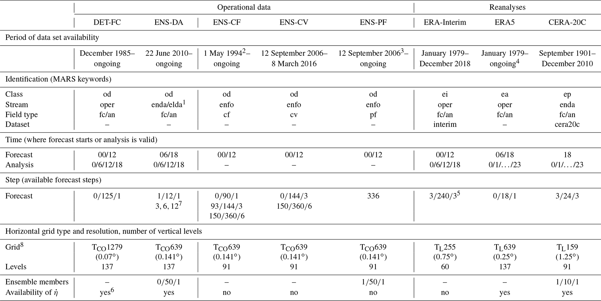
1 From 22 June 2010 to 18 November 2013, ENS-DA was stored in stream ENDA, afterwards in stream ELDA.
2 In existence since November 1992, but the available dates were unregular in the beginning before
1 May 1994.
3 The data set exists from November 1992, but model level data are available only from 12 September 2006 on.
4 Available with a delay of ca. 3 months. Fast track data with shorter delay are
now also available, but subject to possible revisions.
5 For public users, the forecast model level fields are not available.
6 Available as MARS parameter since 4 June 2008.
7 On 11 June 2019, the steps
changed from to the single steps
8 See Table 4 for correspondence of grid types.
Table 2List of the evolution of the spatial resolution of the IFS operational forecasts. Changes are marked in bold. The ensemble data are usually provided with higher resolution for Lag A (1–10 d) than for Lag B (10–15 d). The first part of each entry is the horizontal resolution marked with a “T” for spectral representation; with “T” representing the linear and “TCO” the cubic octahedral representation. The second part, marked with “L”, is the number of vertical model levels. In the case of ensembles, the number N of members is written in front of the resolution as N*. Source: Palmer et al. (1997), Buizza et al. (2003), ECMWF (2019c, e, f, g).
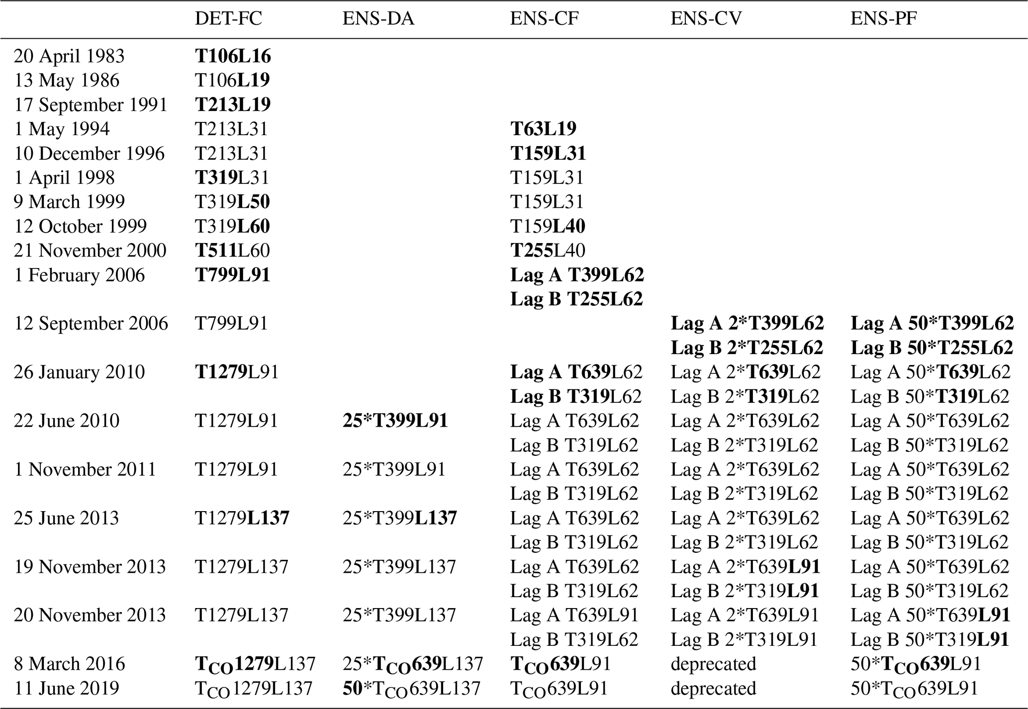
Table 3List of the evolution of forecast steps and forecast start times for data sets DET-FC and ENS-CF. “Lag s” denotes different temporal resolution for forecast ranges s; “#steps” is the total number of steps. Source: ECMWF (2019e)
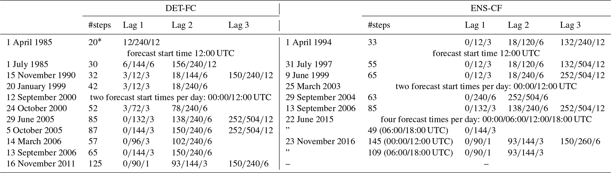
* Only surface fields.
Table 4Approximate correspondences between spectral, Gaussian and latitude–longitude grid resolutions. Source: ECMWF (2017, 2019d, e), Berrisford et al. (2011), Laloyaux et al. (2016). For the spectral grid the truncation number is denoted by “T” where the subscript “q” means quadratic grid and “l” means linear grid. The quadratic grid cannot be selected with flex_extract. The corresponding reduced Gaussian grids are denoted by “N” followed by the number of lines between the pole and the Equator. The new octahedral grid is denoted by “TCO”, meaning “spectral cubic octahedral”; they correspond to a octahedral reduced Gaussian grid, denotes with an “O”.

With the establishment of the Copernicus Climate Change Service (C3S) in March 2019, a new channel for accessing ECMWF reanalysis data, most prominently ERA5 (Hersbach et al., 2020), has been opened. At the same time, access to this data set via the ECMWF Web API was cancelled. While access directly from ECMWF servers is not affected, in local retrieval modes now one has to submit requests to the Copernicus Climate Data Store (CDS), which uses another web API called CDS API; in the background, this API retrieves the public data from dedicated web servers for faster and easier access. Unfortunately, only surface and pressure level data are available in CDS at the moment; this might change in the future. It is possible to pass the request for model levels to the MARS archive even through the CDS interface. This is done automatically since flex_extract is configured to do this. However, experience shows that this access mode is very slow (https://confluence.ecmwf.int/display/CKB/How+to+download+ERA5; last access: 22 June 2020); thus, currently it is not recommend for member-state users.
The flex_extract software package allows the easy retrieval and preparation of the meteorological input files from ECMWF for FLEXPART (and FLEXTRA) and in an automated fashion. The necessary meteorological parameters to be retrieved are predefined according to the requirements of FLEXPART and the characteristics of various data sets. The post-processing after retrieval for the calculations of the flux fields (Sect. 3.6) and the vertical velocity (Sect. 3.7) is also included.
The actions executed by flex_extract (also called “the software package” henceforth) depend on the user group (see Sect. 2.1), the location of execution and the data to be retrieved. There are three possible locations of execution, namely the ECMWF member-state Linux servers, the member state gateway server or a local host. As not all combinations are possible, the result is a total of four different application modes, which are described in Sect. 3.1. Because of the dependencies of flex_extract, the respective application environments need to be prepared in different ways as described in Sect. 3.2. The software package comprises a Python part for the overall control of the processing, including the data extraction, a Fortran part for the calculation of the vertical velocity, KornShell scripts for batch jobs to run on ECMWF servers and bash shell scripts as a user-friendly interface to the Python code. Available settings and input files are described in Sect. 3.4. The output files are divided into temporary files (Sect. 3.8) which are usually deleted at the end and the final output files (Sect. 3.9) which serve as FLEXPART input. An overview of the program structure and the workflow together with an example is given in Sect. 3.3.
The structure of the flex_extract root directory is presented in Table 5; it is completely different than in previous versions. The installation script setup.sh is directly stored under the root directory together with basic information files. Source contains all Python and Fortran source files, each in a separate directory. Flex_extract works with template files, stored in Templates. The online documentation is included in Documentation so that it can also be read offline. The actual work by users takes place in the Run directory. There are the CONTROL_* files in the Control directory, the KornShell job scripts in Jobscripts and, in the case of applying the local mode, also a Workspace directory where the retrieved GRIB files and final FLEXPART input files will be stored. The ECMWF_ENV file is only created for the remote and gateway mode; it contains the user credentials for ECMWF servers. The run.sh and run_local.sh scripts are the top-level scripts to start flex_extract. Like in the previous versions, users can also directly call the submit.py script. There is also a directory For_developers which contains the source files of the online documentation, source files for figures and sheets for parameter definitions.
Table 5Directory structure of the flex_extract v7.1 root directory.

3.1 Application modes
Arising from the two user groups described in Sect. 2.1 and the three possible locations of application, three different user application modes are defined, namely “remote”, “gateway” and “local” mode. However, the local mode is further split in the “local member” and the “local public” mode. A summary of the necessary registration method per mode and user group is outlined in Table 6. An overview of locations and modes is sketched in Fig. 1, and a definition is given in the following list:
- Remote (member)
-
users work directly on ECMWF Linux member-state servers, such as
ecgateorcca/ccb. The software will be installed and run in the users$HOMEdirectory. Users do not need to install any of the additional library packages mentioned in Sect. 3.2 since ECMWF provides everything with an environment module framework. Flex_extract takes care of loading the necessary modules. - Gateway (member)
-
mode is recommended in the case a local member-state gateway server is in place (ECMWF, 2019j), and the user has a member-state account. Job scripts would then be prepared locally (on the gateway server) and submitted to the ECMWF Linux member-state server via the ECMWF web access toolkit
ECaccess. The actual data extraction and post-processing is then done on the ECMWF servers, and the final data are, if selected, transferred back to the local gateway server. The installation script of flex_extract must be executed on the local gateway server. However, this will install flex_extract in the users$HOMEdirectory on the ECMWF server, and some extra set-up is done in the local gateway version. For instructions about establishing a gateway server, please consult ECMWF (2019j) directly. The necessary software environment has to be established before installing flex_extract. - Local member
-
users work on their local machines, which require a similar software environment as the one on ECMWF servers plus the provided web API's as the interface for the MARS archive.
- Local public
-
users can work on their local machines, having fulfilled the software dependencies and having added the ECMWF Web API and the CDS API as the interfaces to the public MARS archive. In this case, a direct registration at ECMWF and CDS is necessary, and all users have to accept a specific licence agreement for each data set which is intended to be retrieved.
Table 6Necessary account registrations per user and application mode for each data set. The registration procedure is indicated by numbers 1–3 and explained below.
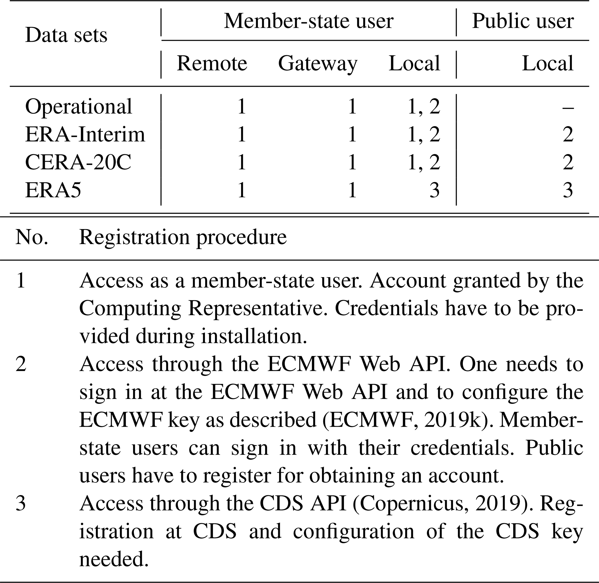
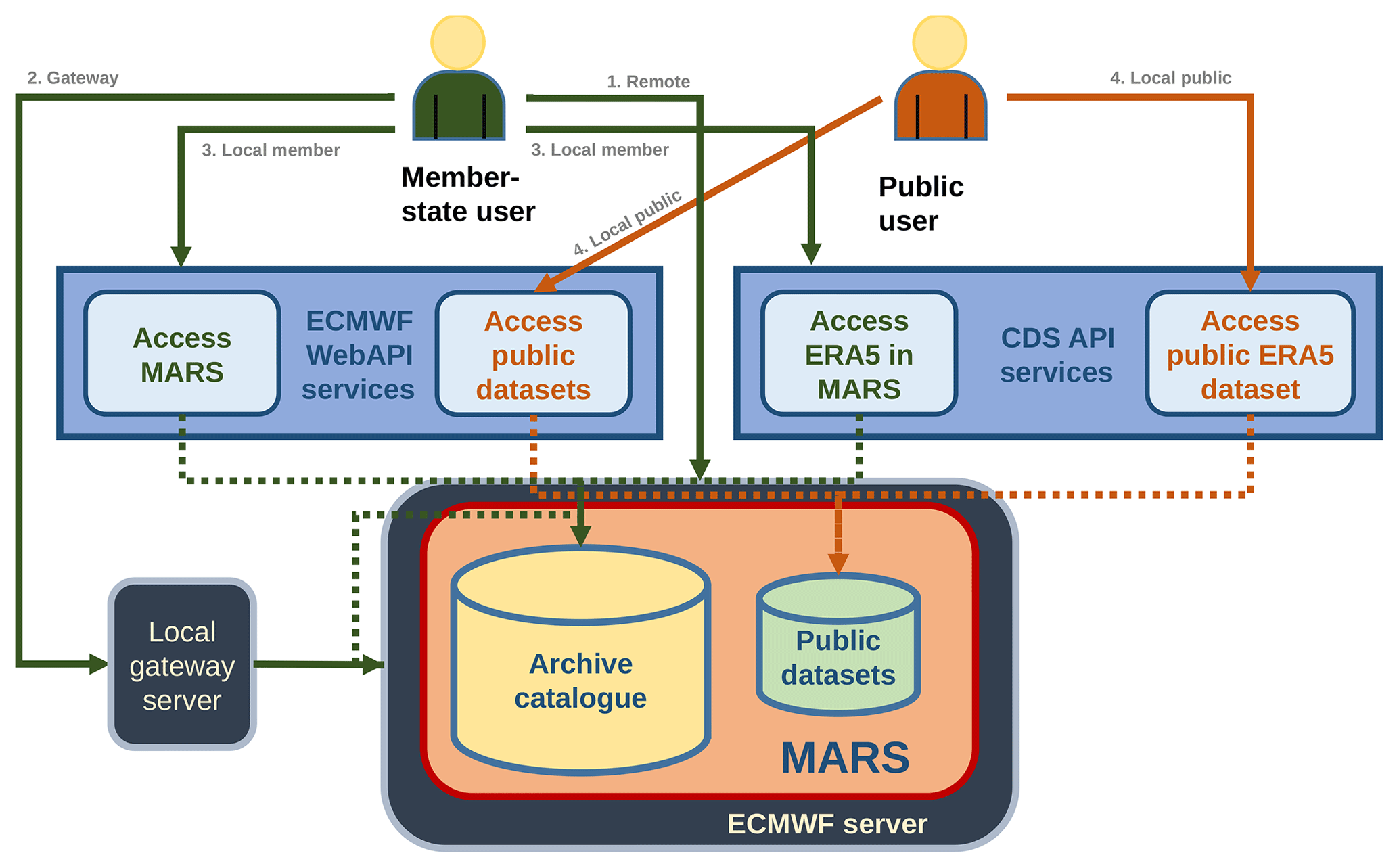
Figure 1Schematic overview of access methods to the ECMWF MARS archive implemented in flex_extract.
3.2 Software dependencies
Software required to run flex_extract depends on the application mode. Basic requirements for all application modes are listed in Table 7.
The local mode requires in addition Python packages ecmwf-api-client and/or cdsapi, depending on the data set to be retrieved, to connect to the MARS archive as Table 6 shows.
Users should make sure that all dependencies are satisfied before starting the installation.
Flex_extract is tested only in a GNU–Linux environment, although it might be possible to use it also under other operating systems.
Table 7Software dependencies for flex_extract in all application modes.
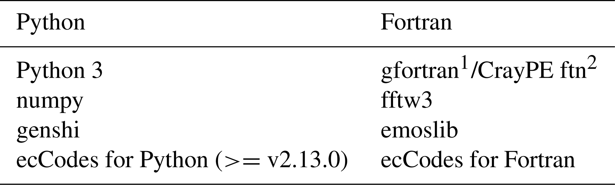
1 Remote mode/gateway mode on ecgate and local mode. 2 Remote mode gateway mode on cca/ccb.
3.3 Program structure
The work of flex_extract can be decomposed into the following three separate tasks:
-
The parameters controlling the retrieval and the data set are set:
this includes reading of theCONTROLfile, command-line arguments and ECMWF user credential file (in the case of remote or gateway mode). Depending on the application mode, flex_extract prepares a job script which is sent to the ECMWF batch queue or proceeds with the tasks 2 and 3. -
Data are retrieved from MARS:
MARS requests are created in an optimized way (jobs split with respect to time and parameters) and submitted. Retrieved data are arranged in separate GRIB files. If the parameterREQUESTwas set to 1, the request is not submitted and only a filemars_requests.csvis created. If it is set to 2, this file is created in addition to retrieving the data. -
Retrieved data are post-processed to create final FLEXPART input files:
after all data are retrieved, flux fields are disaggregated, and vertical velocity fields are calculated by the Fortran programcalc_etadot. Finally, the GRIB fields are merged into a single GRIB file per time step with all the fields FLEXPART expects. Depending on the parameter settings, file transfers are initiated and temporary files deleted.
In task 1, the execution of the code depends on the application mode. In the case of remote or gateway mode (see also Fig. 2), the job script for the ECMWF batch system is prepared and submitted to the batch queue. The program finishes with a message to standard output. In the case of the local application mode, the work continues locally with tasks 2 and 3, as illustrated in Fig. 3.
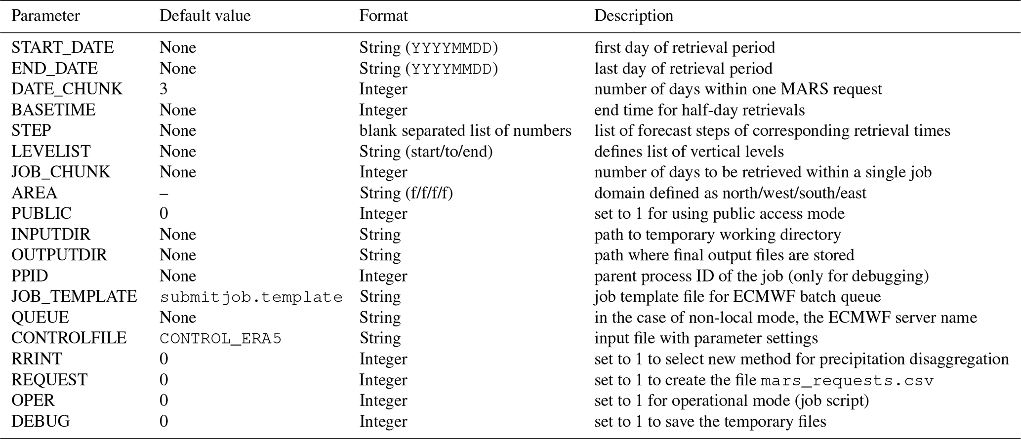
Table 8Overview of CONTROL file parameters. A more detailed description on parameter handling, setting and value ranges is given in the Supplement.
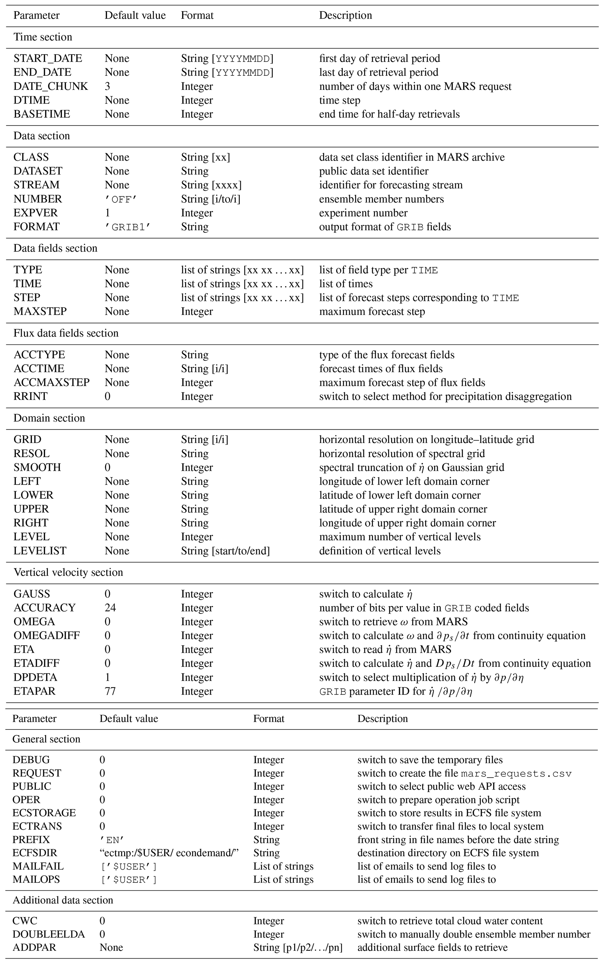
Figure 4 demonstrates the involved input files, execution scripts and connection methods as well as the locations where each step takes place.
The remote and gateway mode both create a job script using the command-line parameters and the content of the specified CONTROL file and then send it to an ECMWF batch queue. In remote mode this happens on an ECMWF server, while the gateway mode uses the local gateway server for the creation and submission of the job. As the job script is executed from whichever of the two modes, it creates the job environment (in particular, the working directory) and starts submit.py to retrieve and post-process the data. Note that this locally started instance of submit.py triggers the workflow of the local mode but uses the MARS client to extract the requested fields from the database. The final output files are sent to the local member-state gateway server only if the corresponding option was selected in the CONTROL file. When flex_extract is used on a local host and in local mode, fields are extracted from MARS using one of the web API's (which sends HTTP requests to ECMWF or CDS) and are received by the local host without storage on ECMWF servers.
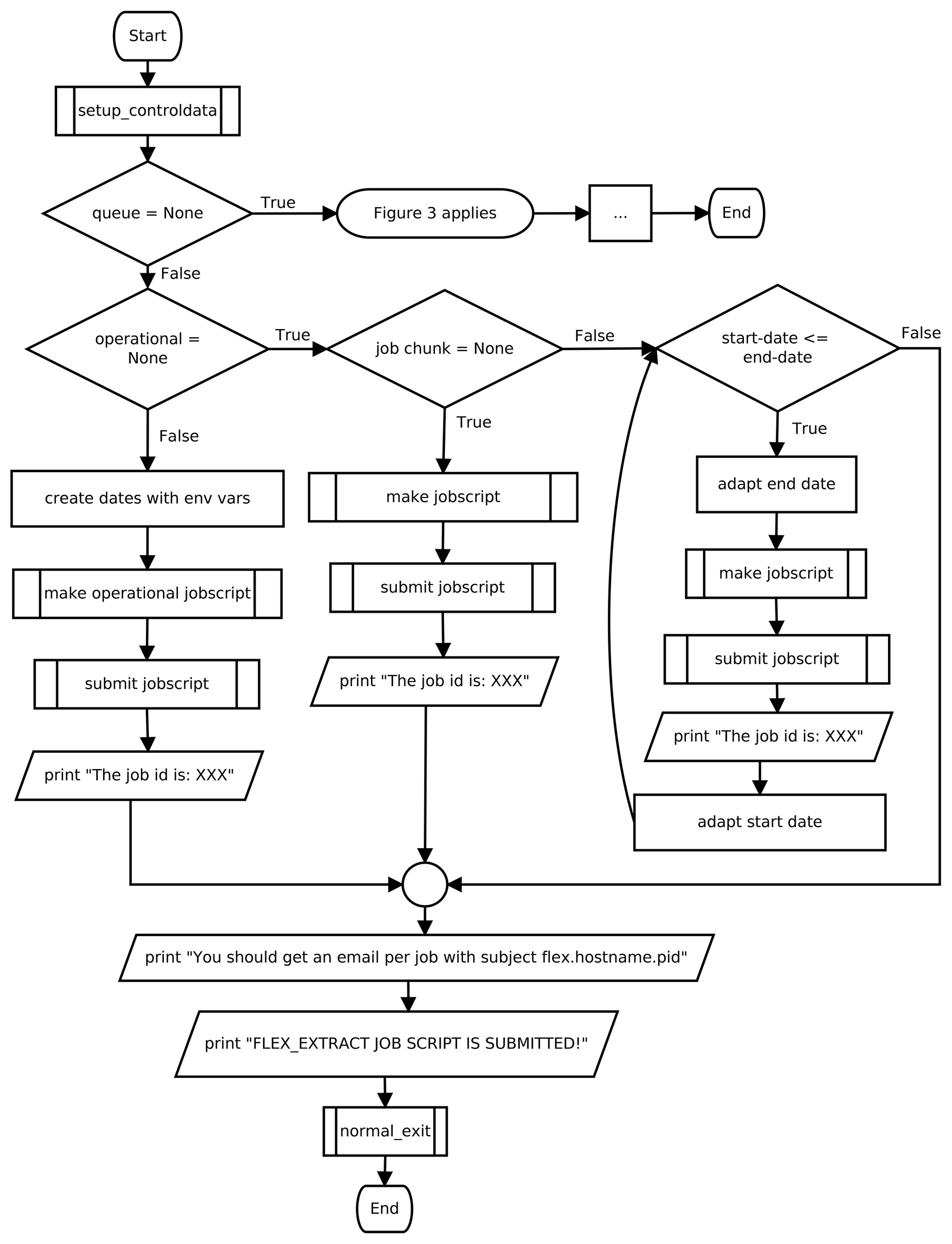
Figure 2Flow diagram for the remote and gateway mode. A job script is created and submitted to the batch queue on an ECMWF server. The job script will then be executed on the ECMWF server to start flex_extract again for retrieving and post-processing of the data. The branch indicated by queue = None refers to the workflow shown in Fig. 3. Trapezoidal boxes mark standard output, simple rectangles mark the execution of sequential instructions, and the rectangles with a side border mark the execution of subroutines. The boxes in diamond form indicate decisions.
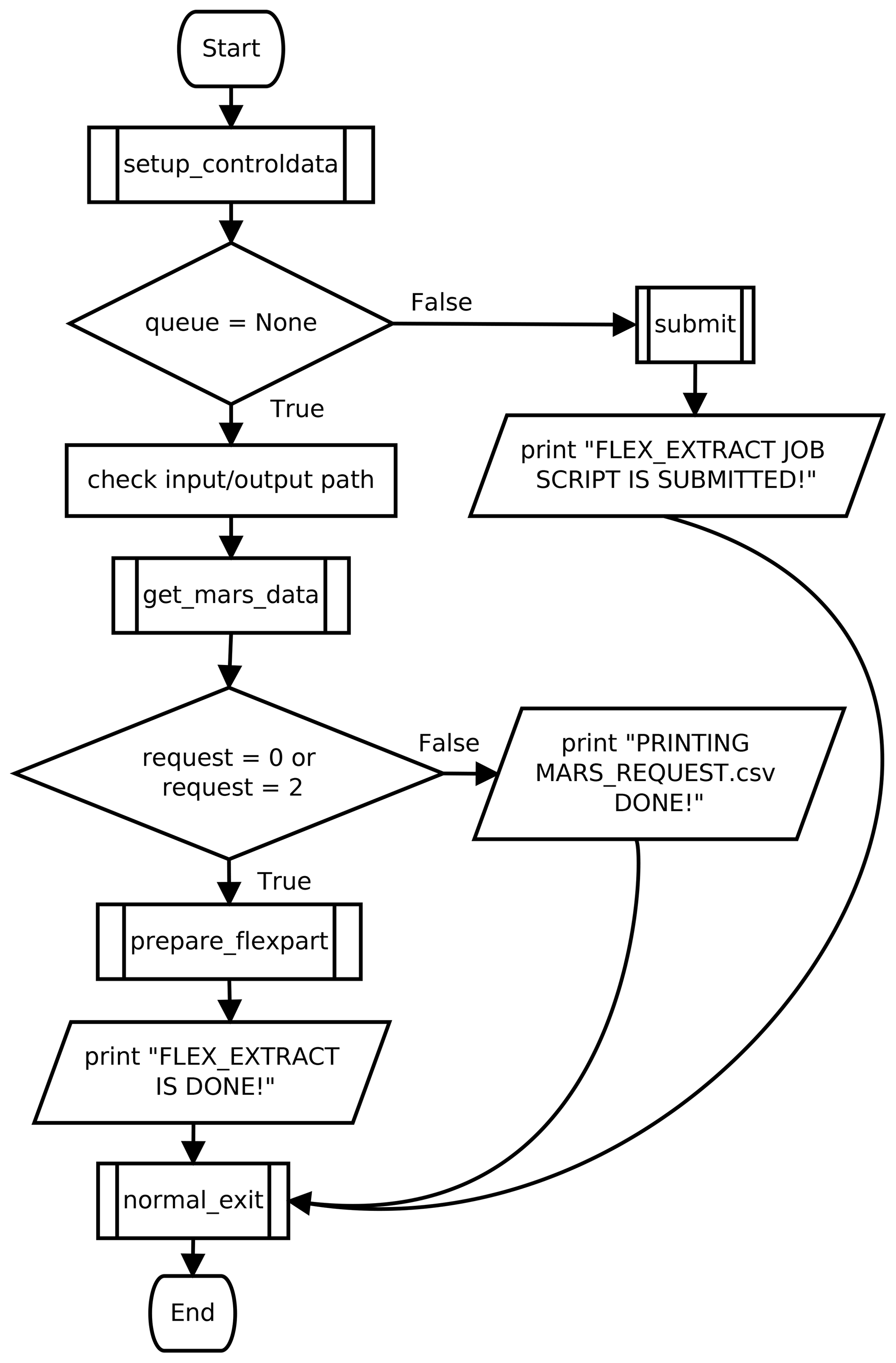
Figure 3Flow diagram for the local application mode. If queue ≠ None, flex_extract was started in remote or gateway mode and Fig. 2 applies. This is marked by the submit block. In the case of request == 1, flex_extract skips the retrieval and post-processing steps and just writes the mars_request.csv file. Within the local mode, the retrieval (get_mars_data) and post-processing (prepare_flexpart) parts are executed. Symbols as in Fig. 2.
3.4 Input files
3.4.1 The CONTROL file
Flex_extract needs a number of controlling parameters. They are initialized by flex_extract with their default values and will be overwritten by the settings in the CONTROL file. Only those parameters which deviate from the default values have to be provided. It is necessary to understand these parameters and to set them to proper and consistent values. They are listed in Table 8 with their default values and a short description. More detailed information, hints about the conditions of settings and possible value ranges are available in the Supplement, partially in Sect. 4 and the online documentation.
Regarding the file content, the first string in each line is the parameter name, the following string(s) (separated by spaces) are the parameter values. The parameters may appear in any order, with one parameter per line. Comments can be added as lines beginning with # sign or after the parameter value. Some of these parameters can be overruled by command-line parameters provided at program call.
The naming convention is CONTROL_<dataset>[.optionalIndications], where the optionalIndications is an optional string to provide further characteristics about the retrieval method or the data set. See Sect. 4 for more details and examples.

Figure 4General overview of the workflows and work locations in the different application modes: (a) remote, (b) gateway and (c) local mode. The files and scripts used in each mode are outlined.
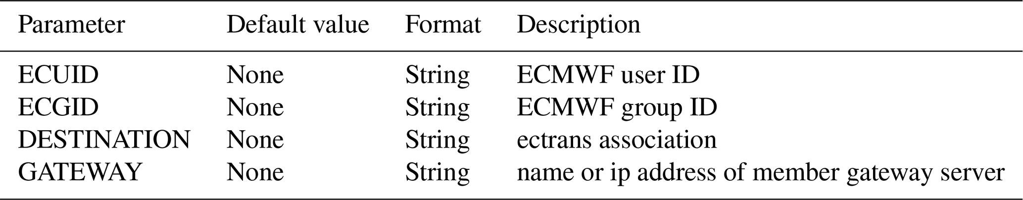
3.4.2 User credential file ECMWF_ENV
In the remote and gateway mode, flex_extract sends job scripts to the batch system of an ECMWF server; thus, it is necessary to provide the user and group name which are given in file ECMWF_ENV. Additionally, this file provides the name of the local member-state gateway server and the destination so that unattended file transfer (https://confluence.ecmwf.int/display/ECAC/Unattended+file+transfer+-+ectrans; last access: 9 September 2019) (ectrans) between ECMWF and member gateway servers can be used. The destination is the name of the so-called ectrans association; it has to exist on the local gateway server.
Table 9Description of the parameters stored in file ECMWF_ENV.
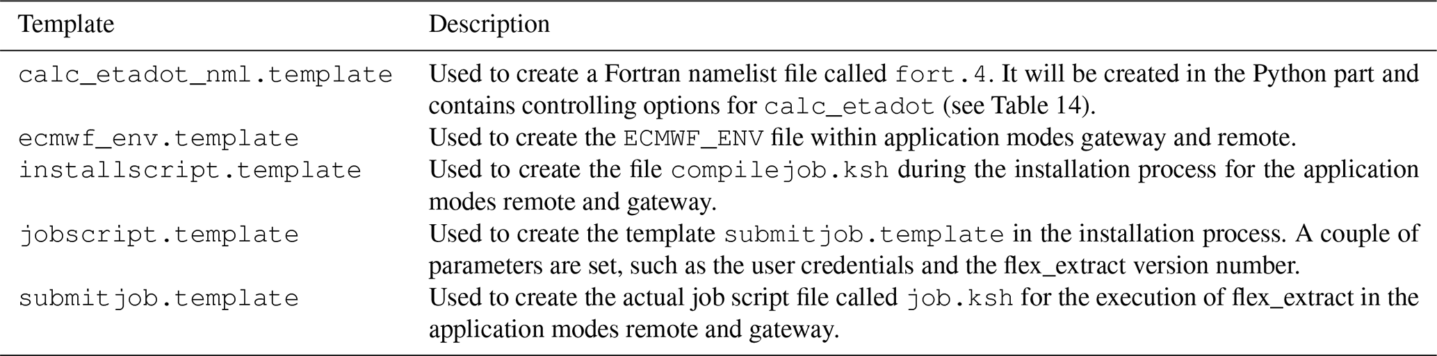
3.4.3 Template files
Some files are highly variable depending on the setting in the other input files. They are created during runtime by using template files. The templates are listed in Table 10.
Flex_extract uses the Python package genshi to read the templates and substitute placeholder by values. These placeholders are marked by a leading $ sign. In the case of the KornShell job scripts, where (environment) variables are used, the $ sign needs to be character quoted by an additional $ sign. Usually, users do not have to change these files.
Table 10Overview of templates used in flex_extract. They are stored in the Templates directory.
3.5 Executable scripts
3.5.1 Installation
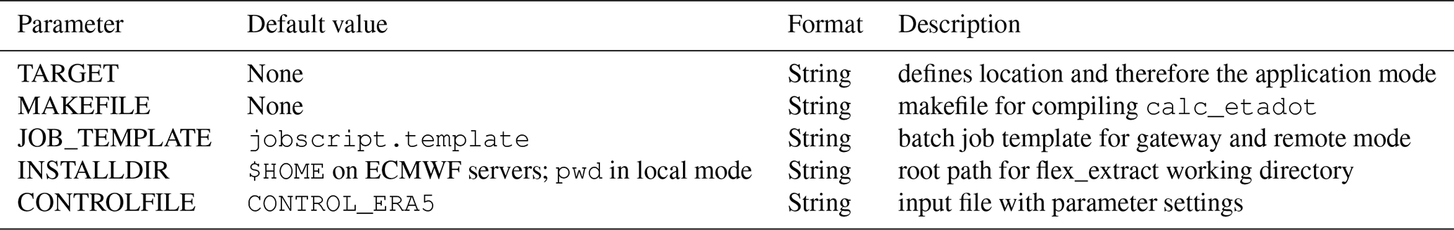
The shell script setup.sh, which is located in the root directory of flex_extract, installs flex_extract. It defines the installation parameters which are defined in Tables 9 and 11 and applies some plausibility checks before it calls the Python script install.py.
The Python script does the installation depending on the selected application mode. In the case of remote and gateway mode, the ECMWF_ENV file is created, the job script template submitjob.template is prepared and stored in the Templates directory, and the KornShell script for compiling the Fortran source code compilejob.ksh is created. After these preparations, a tarball with the core content is created and copied to the target location (ECMWF server or local installation path). Next, the compilejob.ksh is submitted to the batch system of ECMWF servers via ECaccess commands, the tarball is just untarred at the local target location. It compiles the Fortran code, prepares the work environment on ECMWF servers and, in the case of remote/gateway mode, a log file is sent to the user's email address.
Table 11Overview of parameters to be set in the setup.sh script for installation. In remote and local mode for member-state users, the file ECMWF_ENV will be created; hence the parameters from Table 9 must also be set in the setup.sh script.
3.5.2 Execution
The shell script run.sh or run_local.sh starts the whole procedure by calling the Python script submit.py with predefined command-line arguments (see Table 12) from a user section. The Python script constitutes as the main entry point and controls the program flow including the call of the Fortran program. Some of the parameters in run.sh are only needed at the time of the program call, while others are also defined in the CONTROL file. In this case, the values in run.sh take precedence over those from the CONTROL file.
The submit.py script interprets the command-line arguments and, based on the input parameter QUEUE, it decides which application mode is active. In local mode, data are fully extracted and post-processed, while in the remote and gateway mode, a KornShell script called job.ksh is created from the template submitjob.template and submitted to the ECMWF batch system. In the case of the gateway mode, this is done via the local gateway server. The job script sets necessary directives for the batch system, creates the run directory and the CONTROL file, sets some environment variables (such as the CONTROL file name), and executes flex_extract. The standard output is collected in a log file which will be sent to the user email address in the end.
The batch system settings are fixed, and they differentiate between the ecgate and the cca/ccb server systems to load the necessary modules for the environment when submitted to the batch queue. The ecgate server has directives marked with SBATCH (https://confluence.ecmwf.int/display/UDOC/Writing+SLURM+jobs; last access: 10 September 2019) for the SLURM workload manager, the high-performance computers cca and ccb have PBS (https://confluence.ecmwf.int/display/UDOC/Batch+environment%3A++PBS; last access: 10 September 2019) comments for PBSpro. The software environment dependencies mentioned in Sect. 3.2 are fulfilled by loading the corresponding modules. It should not be changed without further testing.
3.6 Disaggregation of aggregated flux data
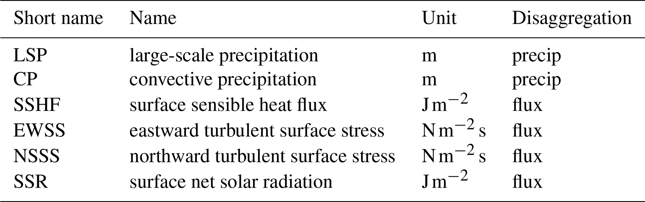
FLEXPART interpolates meteorological input data linearly to the position of computational particles in time and space (Stohl et al., 1998, 2005). This method requires point values in the discrete input fields. However, flux data from ECMWF (as listed in Table 13) represent cell integrals and are accumulated over a time interval which depends on the data set. A pre-processing scheme is therefore applied to convert the accumulated values to point values valid at the same times as the main input fields while conserving the integral quantity with FLEXPART's linear interpolation.
Table 13List of flux fields retrieved by flex_extract and the disaggregation schemes (precip: Eq. 1 or Sect. 3.6.2, flux: Eq. 4) applied.
The first step is to de-accumulate the fields in time so that each value represents an integral in (x, y, t) space. Afterwards, a disaggregation scheme is applied. While the horizontal cell values are simply ascribed to the cell centre, with respect to time, a more complex procedure is needed because the final values should correspond to the same time as the other variables. In order to be able to carry out the disaggregation, additional flux data are retrieved automatically for one day before and one day after the period specified. Note that these additional data are temporary and used only for disaggregation within flex_extract. They are not contained in the final FLEXPART input files.
The flux disaggregation produces files named fluxYYYYMMDDHH, where YYYYMMDDHH is the date. Note that the first and last two flux files do not contain any data.
Note that for operational retrievals which use the BASETIME parameter, forecast fluxes are only available until BASETIME so that interpolation is not possible in the last two time intervals. This is the reason why setting BASETIME is not recommended for regular on-demand retrievals.
3.6.1 Disaggregation of precipitation in older versions
In versions 7.0.x and earlier, a relatively simple method was applied to process the precipitation fields, consistent with the linear temporal interpolation applied in FLEXPART for all variables. At first, the accumulated values are divided by the number of hours (i.e. 3 or 6). For the disaggregation, precipitation sums of four adjacent time intervals (pa, pb, pc, pd) are used to generate the new instantaneous precipitation (disaggregated) value p which is output at the central point of the four adjacent time intervals.
The values pac and pbd are temporary variables. The new precipitation value p constitutes the de-accumulated time series used later in the linear interpolation scheme of FLEXPART. If one of the four original time intervals has a negative value, it is set to 0 prior to the calculation. Unfortunately, this algorithm does not conserve the precipitation within the interval under consideration, negatively impacting FLEXPART results as discussed by Hittmeir et al. (2018) and illustrated in Fig. 5. Horizontally, precipitation is given as cell averages. The cell midpoints coincide with the grid points at which other variables are given, which is an important difference to the temporal dimension. FLEXPART uses bilinear interpolation horizontally.

Figure 5Example of disaggregation scheme as implemented in older versions of flex_extract for an isolated precipitation event lasting one time interval (thick blue line). The amount of original precipitation after de-accumulation is given by the blue-shaded area. The green circles represent the discrete grid points after disaggregation. FLEXPART interpolates linearly between them as indicated by the green line and the green-shaded area. Note that supporting points for the interpolation are shifted by half a time interval compared to the other meteorological fields. From Hittmeir et al. (2018).
3.6.2 Disaggregation for precipitation in version 7.1
Due to the shortcomings described above, a new algorithm was developed by Hittmeir et al. (2018). In order to achieve the desired properties (Hittmeir et al., 2018, p. 2513), a linear formulation with two additional supporting points within each interval is used. The current version of flex_extract implements this algorithm for the temporal dimension. Figure 6 shows how these requirements are fulfilled in the new algorithm for the simple case presented in Fig. 5.
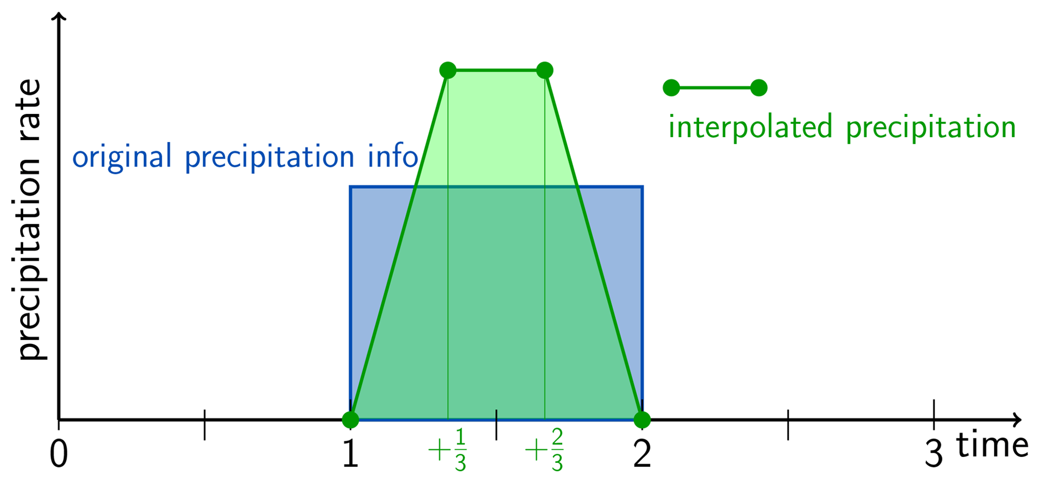
Figure 6As Fig. 5, but with the new interpolation scheme using additional subgrid points. From Hittmeir et al. (2018).
Flex_extract allows one to choose between the old and the new disaggregation method for precipitation. In the latter case, the two additional subgrid points are added in the output files.
They are identified by the parameter STEP, which is 0 for the original time at the left boundary of the interval, and, respectively, 1 and 2 for the two new subgrid points. File names do not change.
FLEXPART up to version 10.4 cannot properly handle this input files generated with the new disaggregation scheme; they would use the third field (second additional subgrid point in time), which would be worse than using the current method.
One of the next minor versions of FLEXPART (probably version 10.5 or
higher) is going to support the scheme.
3.6.3 Disaggregation for the other flux fields
The accumulated values for the other fluxes are first divided by the number of hours and then interpolated to the times of the major fields. The algorithm was designed to conserve the integrals of the fluxes within each time interval when reconstructed with a cubic polynomial. It uses the integrated values F during four adjacent time intervals (F0, F1, F2, F3) to generate a new, disaggregated point value F which is output at the central point of the four adjacent time intervals.
Note that a cubic interpolation was never implemented in FLEXPART. We therefore plan to replace this scheme by an adaption of the scheme used for precipitation, adapted to the situation where both positive and negative values are possible.
3.7 Preparation of vertical velocity
An accurate representation of the vertical velocity is a key component for atmospheric transport models. One of the considerations for the design of FLEXTRA was to work entirely in the native coordinate system of ECMWF's IFS model to minimize interpolation errors. This meant that the same hybrid η coordinate (terrain-following near-ground, approaching pressure levels towards the model top) would be used, which implied using the corresponding native vertical velocity (“”)
rather than the more commonly used ordinary vertical velocity in a simple z system (units of m s−1) or the vertical motion ω of pressure-based systems (unit Pa s−1). For reasons that we cannot reconstruct, however, FLEXTRA did not use strictly, but rather a quantity, which obviously has units of pascals per second.
The code calls this quantity etapoint, not to be confused with etadot. Even though in FLEXPART this concept had to be abandoned in favour of a terrain-following z system to allow a correct implementation of the Langevin equation for turbulent motion, FLEXTRA and FLEXPART share the same requirement for the vertical motion with respect to their input. Over many years, ECMWF would store only the post-processed pressure vertical velocity ω=dp∕dt. Transforming this back to , with approximations and interpolations involved in both operations, leads to vertical velocities that do not fulfil continuity. Therefore, was reconstructed from the fields of divergence using the continuity equation, integrated from the model top downward as described in Simmons and Burridge (1981). In the IFS model, dynamical variables are horizontally discretized by spherical harmonics. It is best to do this on the reduced Gaussian grid that is used in IFS when a grid-point representation is required.
In September 2008, ECMWF started to archive the model's native vertical velocity fields () for the operational analyses and forecasts. This allowed flex_extract to skip the cumbersome reconstruction and directly use this parameter. The number of data that need to be extracted from MARS, the CPU time and the memory requirements are all reduced substantially. The ERA5 and CERA-20C reanalyses also provide . Thus, even though it is possible to use the old method on new data sets, there is no reason to do so and it would be a waste of resources. It is, however, still kept in flex_extract to allow extraction of data from the older data sets, in particular ERA-Interim. In the following, the two methods are briefly characterized.
3.7.1 Reconstruction of the vertical velocity using the continuity equation
The most accurate algorithm for the reconstruction of the native vertical velocity requires the extraction of the horizontal divergence fields and the logarithm of the surface pressure in spectral representation (and thus always global, regardless of the final domain), their transformation to the reduced Gaussian grid (introduced by Ritchie et al., 1995), on which the continuity equation is solved, a transformation back to the spectral space, and finally the evaluation on the latitude–longitude grid desired by users. Especially for high spectral resolution, this is a compute- and memory-intensive process that also takes time, even when making use of OpenMP parallelization. Larger data sets can only be treated on the supercomputer (cca/ccb) but not on ecgate. The code for these calculations is written in Fortran 90.
Alternatively, data can be extracted from MARS immediately on the latitude–longitude grid for the domain desired, and the continuity equation is then solved on this grid, but this method is not as accurate as the calculations on the Gaussian grid, particularly for higher spatial resolutions.
3.7.2 Preparation of the vertical velocity using archived
If the vertical velocity is available in MARS, it only needs to be multiplied with . In the flex_extract version discussed here, this is done by the Fortran program, whose functionality is described below.
3.7.3 Short description of the functionality of the calc_etadot code
A dedicated working directory is used where all input and output files are kept. Currently, the files have names of the form fort.xx, where xx is some number.
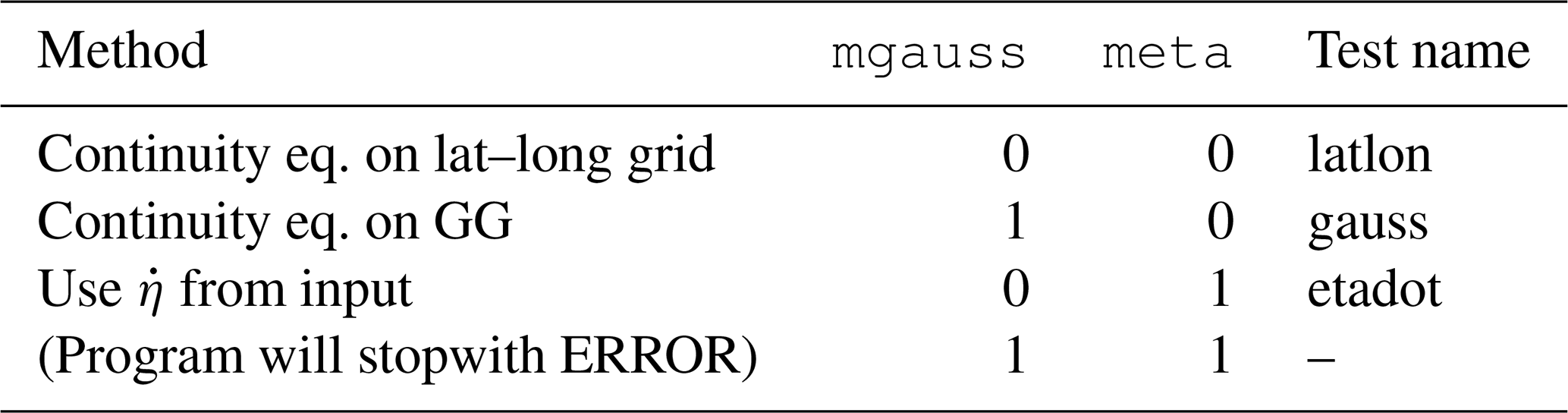
The control file steering the code is fort.4 and has the form of a Fortran namelist. An overview of the options set by this namelist is contained in Table 14. The control file is prepared automatically by the Python code, but some of these parameters appear also as input to the Python part. Note that the selection of the method for obtaining follows the logic laid out in Table 15.
All other input files are data in GRIB format that were retrieved from MARS. The code is using dynamic memory allocation and thus does not need to be recompiled for different data sets.
The code is provided with a set of makefiles. The standard version assumes a typical GNU–Linux environment with the gfortran compiler and the required libraries: OpenMP for parallelization, which is included in the gcc compiler package (libgomp); ecCodes for handling GRIB files; and EMOSLIB for transformation between the various representations of fields. Note that the latter two typically require also so-called developer packages containing the Fortran module files. One may substitute ecCodes with its predecessor GRIB_API, if ecCodes is not available.
It is assumed that these libraries have been installed as a package from the distribution and thus are at their standard locations and compatible with the gfortran compiler (if not, the makefile library and include paths need to be adapted). There is one makefile called makefile_fast with optimization that is used for production. In addition, there is makefile_debug which is optimized for debugging. There are also makefiles for the ECMWF servers cca/ccb and ecgate.
Table 14Overview of options controlling calc_etadot. Note that the resolution of the latitude–longitude grid is given implicitly by the grid dimensions and extent.
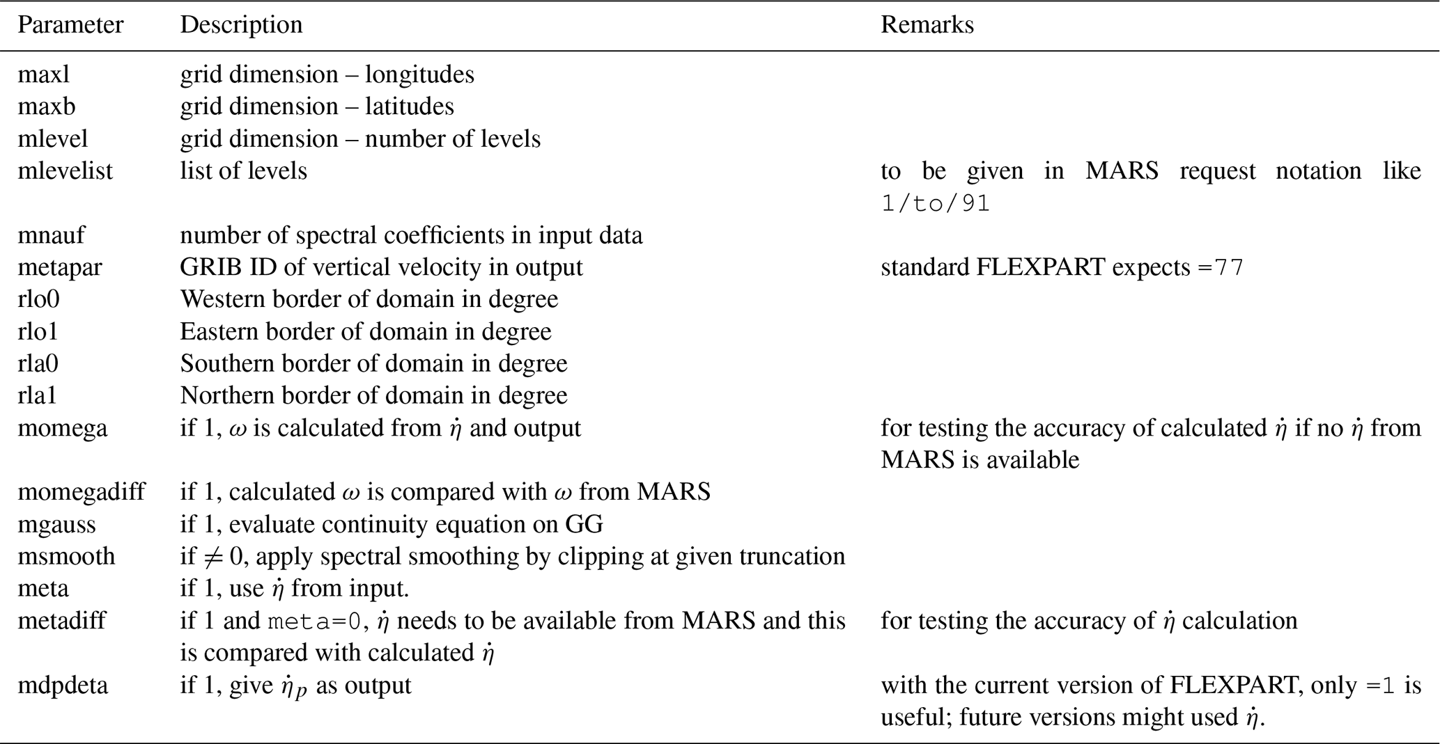
Table 15Determination of the method for obtaining in calc_etadot as a function of control parameters (see also Table 14). GG stands for Gaussian grid. The names of the corresponding regression tests (see Sect. 5.4) are also given
If the program finishes successfully, the last line written to standard output is SUCCESSFULLY FINISHED calc_etadot: CONGRATULATIONS, which is useful for automated checking of the success of the run. The output file into which the fields of and the other three-dimensional variables (temperature, specific humidity, u and v components of the wind – not the recently introduced cloud water variable) are combined is fort.15; it is a GRIB file.
The code also foresees options for certain checks where different forms of the vertical velocity are obtained, statistically compared, and also written out (see Table 14). These options were used for quality control in the development process and should not normally be activated by users.
Currently, the code also unifies the three-dimensional fields extracted from MARS and stored in separate GRIB files with the calculated vertical velocity by writing out all fields into a single GRIB file; later this is unified with the 2D fields and the new 3D parameters such as cloud water and written out into a final single GRIB file as required by FLEXTRA and FLEXPART.
3.8 Temporary output files
These temporary output files are usually deleted after a successful data extraction. They are only kept in debugging mode, which is the case if the DEBUG parameter is set to true.
3.8.1 MARS GRIB files
All extracted meteorological fields from MARS are in GRIB format and stored in files ending with .grb. MARS requests are split in an optimized way to reduce idle times and considering the limit of data transfer per request. The output from each request is stored in one GRIB file whose name is defined as <field_type><grid_type> <temporal_property><level_type>.<date>. <ppid>.<pid>.grb.
The field type can be analysis (AN), forecast (FC), 4d variational analysis (4V), validation forecast (CV), control forecast (CF) and perturbed forecast (PF). The grid type can be spherical harmonics (SH), Gaussian grid (GG), output grid (OG) (typically lat–long) or orography (_OROLSM), while the temporal property distinguishes between an instantaneous field (__) or an accumulated field (_acc). Level types can be model (ML) or surface level (SL), and the date is specified in the format YYYYMMDDHH. The last two placeholders are the process number of the parent process of submitted script (ppid) and the process number of the submitted script (pid). The process IDs are incorporated so that the GRIB files can be addressed properly in the post-processing.
3.8.2 MARS request file
This file contains a list of the MARS requests from one flex_extract run, with one request per line. This is an optional file users are able to create in addition to full extraction; it can also be created without actually extracting the data, which is useful for test purposes. Each request consists of the following parameters, whose meaning is explained in Table 8, explained in more detail in the Supplement, or are self-explanatory: request number, accuracy, area, dataset, date, expver, Gaussian, grid, levelist, levtype, marsclass (alias class), number, param, repres, resol, step, stream, target, time and type. The parameters Gaussian (which defines whether the field is regular or a reduced Gaussian grid), levtype (which distinguishes between model levels and surface level) and repres (which defines the grid type – SH, GG, OG) are internal parameters not defined as any available input parameter.
3.8.3 Index file
The index file is called date_time_stepRange.idx. It contains indices pointing to specific GRIB messages from one or more GRIB files, so Python can easily loop over these messages. The messages are selected with a predefined composition of GRIB keywords.
3.8.4 Files with forecast vertical flux data
The flux files, in the format flux<date>[.N<xxx>][.<xxx>], contain the de-accumulated and disaggregated flux fields which are listed in Table 13. The files are created per time step with the date being in the format YYYYMMDDHH. The optional block [.N<xxx>] marks the ensemble forecast, where <xxx> is the ensemble member number. The second optional block [.<xxx>] marks a long forecast (see Sect. 3.9.2) with <xxx> being the forecast step.
Note that, in the case of the new disaggregation method for precipitation, two new subintervals are added in between each original time interval. They are identified by the forecast step parameter STEP, which is 0 for the original time interval and 1 or 2 for the two new intervals respectively.
3.8.5 fort.* files
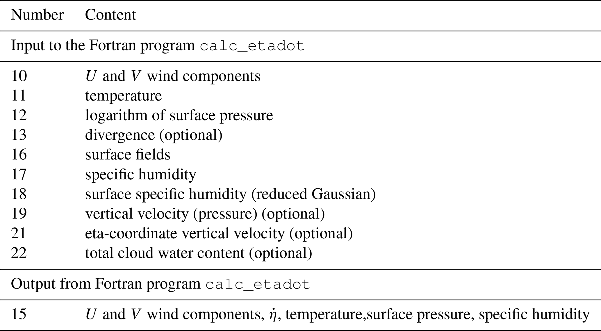
There are a number of input files for the calc_etadot Fortran program named fort.xx, where xx is the number which defines the meteorological fields stored in these files. They are generated by the Python part of flex_extract by just splitting the meteorological fields for a unique time step from the *.grb files. Table 16 explains the numbers and the corresponding content. Some of the fields are optional and are retrieved only with specific settings; for example the divergence is retrieved only if is not available in MARS, and the total cloud water content is an optional field for FLEXPART v10 and newer. The output of calc_etadot is file fort.15.
Table 16List of fort files generated by the Python part to serve as input for the Fortran program and the output file of calc_etadot. If the optional fields were not extracted, the corresponding files are empty.
3.9 Final output – FLEXPART input files
The final output files are the FLEXPART input files containing the meteorological information. FLEXPART expects one file with all relevant fields per time step. Tables 17 and 18 list all of the meteorological fields that flex_extract retrieves and FLEXPART expects. The naming of these files depends on the extracted data. In the following sections we describe the differences and how the file names are built.
Table 17List of model level parameters FLEXPART requires to run and the availability in the different data sets (ECMWF, 2019e, i). The cloud-water content fields are optional. The divergence and logarithm or surface pressure fields are only necessary for the calculation of the vertical velocity when is not available directly. These fields are not transferred to the FLEXPART input files. FC stands for “forecast” and AN for “analysis”.
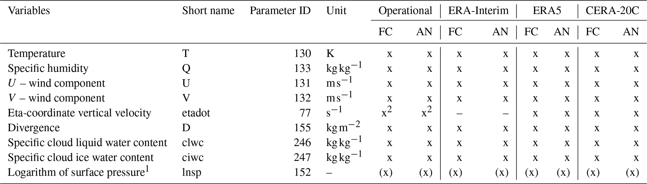
1 Only available on model level 1. 2 Available from 4 June 2008 onward.
Table 18List of surface level parameters FLEXPART requires to run and their availability from different data sets (ECMWF, 2019e, i). FC stands for “forecast” and AN for “analysis”. Special or future versions of FLEXPART or pre/post-processing software may require additional surface level fields which are not listed here.
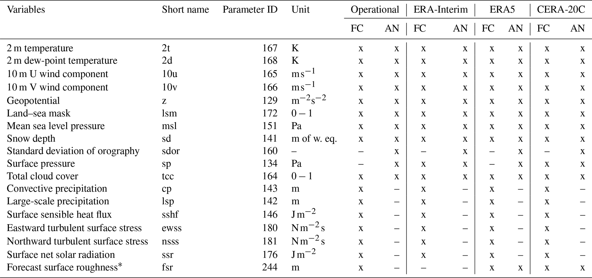
* Necessary in CERA-20C due to missing surface roughness parameter.
3.9.1 Standard output files
The standard file names have the format <prefix>YYMMDDHH, where the <prefix> is by default defined as EN and can be redefined in the CONTROL file. Each file contains all fields on all selected levels on a latitude–longitude grid as needed by FLEXPART.
There is one file per time step, and YYMMDDHH indicates the date and hour for which the fields are contained in the file.
Analysis and forecast times with their corresponding forecast steps are summarized to the actual times.
If not otherwise stated, model-level fields are in GRIB2 format and surface fields in GRIB1.
When CERA-20C data are retrieved, the date format is changed to YYYYMMDDHH.
3.9.2 Output files for long forecasts
For a long forecast, where only forecast fields are retrieved for more than 23 h, a different naming scheme has to be applied to avoid collisions of time steps for forecasts of more than one day. This case is defined as long forecast mode, and file names are defined as <prefix>YYMMDD.HH. <FORECAST_STEP>.
The <prefix> is, as in the standard output files, EN by default and can be redefined in the CONTROL file. In this case, the date format YYMMDD does not include the hour. The HH represents the starting time (base time) of the forecast. The FORECAST_STEP is a three-digit number which represents the forecast step in hours.
3.9.3 Output files for ensemble predictions
If flex_extract retrieves ensemble members, multiple fields result for each meteorological variable (the ensemble members) at a single time step. They are distinguished by the GRIB parameter NUMBER.
All fields of one ensemble member are collected together in a single file per time step. The standard file names are supplemented by the letter N for “number” and the ensemble member number in a three-digit format such as <prefix>YYMMDDHH.N<ENSEMBLE_MEMBER>.
3.9.4 Additional fields with new precipitation disaggregation
The new disaggregation method for precipitation fields produces two additional fields for each time step and precipitation type. They contain the subgrid points in the corresponding original time intervals as described above in Sect. 3.6.2. The two additional fields are marked with the STEP parameter in the GRIB messages, set to “1” and “2”, respectively. The output file names do not change in this case.
As in earlier versions of the software package, it is still possible to directly start flex_extract with the Python script submit.py. An overview of its current command-line arguments is available through ./submit.py - -help.
Please note that when flex_extract is started in local mode, the parameter INPUTPATH in the run_local.sh script must be set so that each retrieval uses a unique directory to avoid mixing of data files.
There are two more entry points into flex_extract which can be used for debugging; they are described here for the sake of completeness: the Python scripts getMARSdata.py and prepare_flexpart.py. In the standard way of running flex_extract, they are both imported as modules (as shown in Fig. 3), but they can also be used as executable programs. The script getMARSdata.py controls the extraction of ECMWF data, while prepare_flexpart.py controls the post-processing. It may happen that the procedure terminates unexpectedly during the post-processing due to time limits on ECMWF servers. In this case, the prepare_flexpart.py script can be used to redo the complete post-processing, bypassing the need to retrieve the data from MARS again.
4.1 Example CONTROL files
The file CONTROL.documentation provides a collection of the available parameters grouped in sections together with their default values. Users can start from this file to define their own set-up or use one of the example CONTROL files as a template (in flex_extract_v7.1/Run/Control/). For each data set (see Sect. 2.2), a basic example CONTROL file is provided with some additional variations in, for example, horizontal and temporal resolution, field type, method for vertical velocity or duration of forecasts. The variations are specified at the end of the file name (CONTROL_<dataset>[.optionalIndications]) as an optional string.
The usage section in the online documentation provides more details on how to set the CONTROL file parameters for specific applications. For example, CONTROL file names which end with .public are for public users. They have the specific parameter DATASET for CERA-20C and ERA-Interim data sets to identify the public version in MARS. For ERA5, this parameter is not needed, and thus public users may use any ERA5 file for extraction.
For the atmospheric high-resolution data sets, indicated by OD, the optional string contains information of the stream (OPER, ENFO, ELDA), the field type of forecasts (FC, CF, CV, PF, 4V), the method for extracting the vertical velocity (eta or gauss), and other aspects such as long forecasts (36hours), operational half-day retrievals (basetime or twicedaily), temporal resolution (1hourly or 3hourly) or different horizontal resolutions with global vs. limited-area domains (highres).
4.2 Changes in CONTROL file parameters in comparison to previous versions
With version 7.1, all CONTROL file parameters are initialized with default values. Thus, only those which need to be changed to identify the data set to be retrieved have to be set in the CONTROL file.
In earlier versions, each parameter name contained the leading string M_; this was removed for version 7.1 but is still accepted for compatibility.
The grid resolution had to be provided in 1∕1000 of a degree before, while now it can be provided also as a decimal number. Flex_extract is able to identify the correct setting of the GRID parameter in combination with the domain-specific settings.
It is now also possible to reduce the number of data values for the combination of TYPE, TIME and STEP parameters to the actual temporal resolution. Previous versions expected to have 24 values per parameter, one for each hour of the day, even if only 3-hourly data were requested, as shown in the following example.
DTIME 3
TYPE AN AN AN AN ... AN AN AN AN
TIME 00 01 02 03 ... 20 21 22 23
STEP 00 00 00 00 ... 00 00 00 00
The more intuitive solution of providing the data for the time steps to be retrieved leads, in this example, to eight data values per parameter for a 3-hourly retrieval.
DTIME 3
TYPE AN AN AN AN AN AN AN AN
TIME 00 03 06 09 12 15 18 21
STEP 00 00 00 00 00 00 00 00
This leads to four values for a 6-hourly retrieval.
DTIME 6
TYPE AN AN AN AN
TIME 00 06 12 18
STEP 00 00 00 00
The only necessity is a consistent setting of the DTIME parameter which defines the temporal resolution. For backward compatibility, DTIME may be coarser than the number of temporal points provided in TYPE, TIME and STEP but not finer.
With this version of flex_extract, it is possible to retrieve data sets with analysis fields at every hour (such as ERA5 and CERA-20C); therefore, it was necessary to introduce new parameters related to flux fields defining the forecast type (ACCTYPE), time (ACCTIME) and step (ACCMAXSTEP) specifically for the flux fields (accumulated quantities). For daily ERA5 retrievals, which need up to 12 h forecasts twice a day for the flux fields, these parameters would be the following.
ACCTYPE FC
ACCTIME 06/18
ACCMAXSTEP 12
Several new parameters were introduced which work as switches. Among the more important ones are REQUEST in order to write the settings in the MARS requests to an output file mars_requests.csv and CWC to trigger the additional retrieval of cloud liquid and ice water content.
DOUBLEELDA can be used to double the number of ensemble members if only 25 members are available from the ELDA stream. These additional members are calculated by subtracting from each existing ensemble member twice the amount of the difference between the ensemble member and the control run.
To distinguish between the old and new precipitation disaggregation scheme, the switch parameter RRINT was introduced. Setting it to 1 indicates that the new scheme is used; 0 selects the old scheme.
4.3 Scientific considerations
First of all, users should be aware of the different nature of operational and reanalysis data sets (see Table 1). Operational data have been available since the start of ECMWF's operational forecasts and are influenced by frequent changes in the IFS model, for example with respect to model physics and resolution. Reanalysis data sets were created using a single IFS model version throughout the whole period covered. More precisely, the CERA-20C data set (with 91 vertical levels, 1.25∘ horizontal and 3 h temporal resolution) has a lower resolution but covers a very long period (from 1901 to 2010) and will thus be suitable for certain climate applications. The ERA-Interim data set (with 60 vertical levels, a medium resolution of 0.75∘ horizontally and 3 h temporally) was the standard ECMWF reanalysis until recently, but without having been stored in the MARS archive, making retrievals computationally demanding as it needs to be reconstructed from the horizontal winds through the continuity equation. The new ERA5 data set has the highest resolution (0.25∘ horizontally and 1 h temporally, 137 vertical model levels) and includes . Users are encouraged to use ERA5 data rather than the ERA-Interim data set (production ended in August 2019). In addition to its better resolution, ERA5 covers a longer period than ERA-Interim, provides uncertainty estimates with a 10-member ensemble data assimilation, and uses a newer IFS model version (ECMWF, 2019l).
With respect to the relation between temporal and spatial resolution, it is important to consider the use in FLEXPART and their influence on numerical errors. It is not useful to apply high horizontal resolution in combination with, for example, 6-hourly temporal resolution, as in such a case small fast-moving structures are resolved in space, but their movement will not be properly represented. Interpolation will not let the structures move but rather jump from their position at time t to that at time t+6 h if the displacement between two subsequent times where fields are available is comparable to or larger than their characteristic width along to the phase speed. Users can orient themselves looking at the spatial and temporal resolutions at which ECMWF provides reanalysis data and the sample CONTROL files.
On the other hand, one has to keep in mind the requirements of the FLEXPART application. For a climatological study on global scales, a horizontal resolution of 0.5 or 1∘ could be a reasonable choice, whereas tracking point releases in complex terrain would call for the best available resolution.
Attention should also be paid to the model topography and the land–sea mask. Due to limited resolution, a coastal site with a given geographical coordinate could be over water in the model. Then it might be better to shift the coordinates of a release or receptor point in FLEXPART slightly. Another aspect is that the smoothed representation of the topography could mean that the model topography is above or below the real height of a site. It is therefore important to select the proper kind of z coordinate in the FLEXPART RELEASES file. As a compromise, one can place a release location at a height between real and model topography (for mountain sites which are usually lower in the model topography than in reality). In such cases, it is strongly recommended to retrieve the model topography and land–sea mask manually and investigate them carefully before deciding on the FLEXPART set-up details, or even before retrieving the full meteorological data set, as one might come to the conclusion that one with better resolution should be used.
The vertical levels used in FLEXPART follow a hybrid η coordinate system. This is much more efficient than pure pressure levels since hybrid η coordinates follow the terrain near ground and approach pressure levels towards the model top. In this way, the lower boundary condition of a flow parallel to the surface is easy to fulfil, whereas pressure levels do not follow the terrain (Stohl et al., 2001). At higher levels, however, the pressure coordinate is more appropriate as flows are mostly horizontal. It also better allows the assignment of a higher vertical resolution to the lowest part of the atmosphere.
ECMWF data sets either directly provide the variable (set ETA and DPDETA to 1; see CONTROL files with eta in their names) or include the data needed to reconstruct it (set GAUSS to 1; see CONTROL files with gauss in their names) accurately. This is a big advantage of ECMWF data compared to other data sources, most notably the NCEP model data, which are publicly available only on pressure levels.
Attention should be paid to the number of vertical model levels to be extracted and used in FLEXPART, as the computational cost of the FLEXPART verttransform subroutine (reading and preparing meteorological input) increases with the third power of the number of vertical levels. Thus, only data that are really needed for the application (e.g. troposphere, or troposphere and lower stratosphere) should extracted. File , for example, retrieves a limited domain with high horizontal (0.2∘) and 1-hourly temporal resolution with levels up to, approximately, 100 hPa by setting LEVELIST to 60/TO/137.
Operational data sets and ERA-Interim have analysis fields at 6 h (00:00/06:00/12:00/18:00 UTC) or 12 h (00:00/12:00 UTC) intervals. The gaps in between can be filled with forecast fields. Mixing analysis and forecast fields should be done by considering at which time steps the differences between two IFS run segments will be the smallest. For example, using all four analysis fields together with forecasts starting at 00:00 and 12:00 UTC would imply that the 06:00 UTC and 18:00 UTC fields would not be consistent with the fields 1 h before and after that hour, respectively. This should be avoided by using only 00:00 and 12:00 UTC analysis fields and the forecast fields for +1 to +11 h for the forecasts starting at times 00:00 and 12:00 UTC, respectively (note that forecasts from the intermediate analyses at 06:00 and 18:00 UTC are not archived). See file CONTROL_OD.OPER.FC.eta.global for an example.
To assure a certain quality of a piece of software, testing is at least as important as developing the code itself. Adding new functionalities requires the development of new tests to identify possible bugs or to show that the code works under specified conditions. As a consequence, output from the tests conducted with the preceding version can be used to verify that there are no unexpected side effects. This is called regression testing (Beizer, 1990; Spillner, 2012). As the functionality of the software changes, tests need to be updated or expanded as well.
For this flex_extract version, code refactoring was at the core of the development, and a number of regression tests were developed for that. In addition, a first set of unit tests (Sect. 5.1), which also serve as a kind of regression test, have been developed within the refactoring process as they are the established best practice in software engineering to investigate small code blocks. Furthermore, we defined test cases to compare the outcome of two flex_extract versions after three different stages of the retrieval process: (1) the MARS requests prepared (Sect. 5.2), (2) the vertical velocity obtained with the different options of calculation (Sect. 5.4), and (3) the final output files in GRIB format (Sect. 5.3).
In addition, generic tests were performed by applying flex_extract with predefined CONTROL files (Sect. 5.5) which are distributed with the software package to serve as examples for the typical applications.
Finally, some code metrics were determined to track quantitative quality aspects of the code. The combination of all of these tests establishes a sustainable testing environment, which will benefit the future development process. The testing environment is not directly relevant for users of flex_extract.
5.1 Unit tests
Unit tests are used to test the smallest pieces of code (single code blocks) independently to identify a potential lack of functional specification (Beizer, 1990). Applying unit tests does not guarantee error-free software; rather it limits the likelihood of errors. Once the tests are written, they serve also as a kind of documentation and to protect against alteration of the functional behaviour by future code changes (Wolff, 2014). In this sense, they are also a kind of regression test.
For the current version of flex_extract, we prepared a first set of unit tests for functions which were designed or partly refactored to be testable code blocks. Our intention is to increase the number of unit tests in the future and to further refactor some still rather complex functions into smaller ones (see also Sect. 5.6 or the Supplement for identifying complex functions).
5.2 Regression testing for MARS requests
The parameters in the MARS requests produced by flex_extract are a key component of the extraction process. Flex_extract v7.1 contains a test to compare the content of MARS requests as produced by two versions. It checks whether the number of columns (parameters) in the request files (see Sect. 3.8.2) is unchanged, whether the number of requests is equal, and whether the content of the request is identical (except for the desired differences and the environment-dependent data such as paths).
The MARS request files for the current version in use are generated automatically at runtime without actually retrieving the data, while the files for the reference version have to be in place before. Since the MARS request files are grouped by version and are saved, the number of reference data sets will grow with each new version.
5.3 Regression testing for GRIB files
The final product of flex_extract, the FLEXPART input files in GRIB format (see Sect. 3.9), should be equal between the previous and the current version, apart from the new or modified features. Since there is always a possibility of having tiny (insignificant) deviations in the actual field values when retrieving at different points in time (changes in the environment, library versions, computational uncertainties, etc.), the focus of this test lies in the files themselves and the GRIB message headers, which should not be different. Future improvements may also test for value differences considering a significance threshold.
A regression test was created which compares the GRIB files produced by two versions with respect to the number of files produced, the file names, the number of GRIB messages per file, the content of the GRIB message header, and statistical parameters for the data themselves. If differences are reported, the developer has to judge whether they are expected or indicate a problem.
5.4 Functionality and performance tests for the Fortran code
Regression tests were set up to reflect the three possibilities for obtaining the vertical velocity listed in Table 15. In addition to a basic test for each, enriched tests are implemented where all checks and additional outputs are activated (names with appended all). These tests use a pre-specified small domain (, 11 levels) and low spectral resolution (T159) and thus run quite fast. As high spectral resolution and a large domain may pose specific problems, and as it will be relevant to watch the runtimes, additional high-resolution tests have been created for the gauss and etadot cases with a domain covering the Northern Hemisphere and all 137 vertical levels. The gausshigh test uses a grid spacing of 0.25∘ and the corresponding spectral resolution of T799; the etadot case uses 0.1∘ and T1279.
5.5 Generic test using predefined CONTROL files
Flex_extract comes with a set of CONTROL files, which can be found in the flex_extract_v7.1/Run/Control directory; executing flex_extract with each of them constitutes a generic test which ensures that the data extraction works for all typical applications.
5.6 Code metrics
Metrics for the maintainability and complexity of code as well for the documentation are a useful tool for developers who should aim at maintaining or reaching good scores in these metrics. For the Python code of flex_extract, a number of metrics were calculated for the previous version 7.0.4 and the current version 7.1. This section summarizes the metrics and their main findings. More details can be found in the Supplement.
Basic metrics, taken from Lacchia (2019) and calculated with the Python package radon (Lacchia, 2019), are
-
the total number of lines of code (
LOC), -
the number of logical lines of code (
LLOC), -
the number of source lines of code (
SLOC), -
the number of (single) comment lines (
comments), -
the number of lines in multi-line comment strings (
multi), and -
the number of blank lines (
blank),
with the following relation between these numbers:
The comparison shown in Table 19 indicates a significant increase not only in the logical lines of code but even more in comment and multi, mostly representing an improvement of in-line documentation by splitting large code blocks into smaller ones, each with a new docstring. A so-called docstring is a specific multi-line comment for the documentation of functions, methods and classes, describing their input and return values, which can be read by tools for automatic generation of a separate documentation.
For the refactorization of code blocks, additional code for new features, and compliance with certain code style rules (e.g. maximum length of lines), about 1000 lines of pure code were added. The ratio of comment lines (multi + comment) to source-code lines (SLOC) grew from 20 % to 117 %.
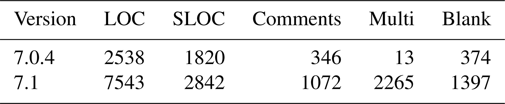
A further metric for code quality is the so-called cyclomatic complexity (CC), also called the McCabe metric (Sneed et al., 2010). It is equal to the number of linearly independent paths through the control flow graph of the code or the number of decisions plus one. A lower CC score indicates a lower complexity, which is deemed an advantage. Table 20 gives an overview of the rank definitions. Regarding code testing, CC provides a lower-bound number of how many test cases (unit tests) are necessary to provide complete path coverage (Beizer, 1990).
In general, it is said that the score should be less than or equal to 10, corresponding to rank A and B. From the statistical point of view, only 10.3 % of flex_extract version 7.1 code blocks have higher complexity, while in version 7.0.4 this was the case for 30.8 %.
Table 20Ranks of cyclomatic complexity (CC) taken from the manual of the Python package radon (Lacchia, 2019).
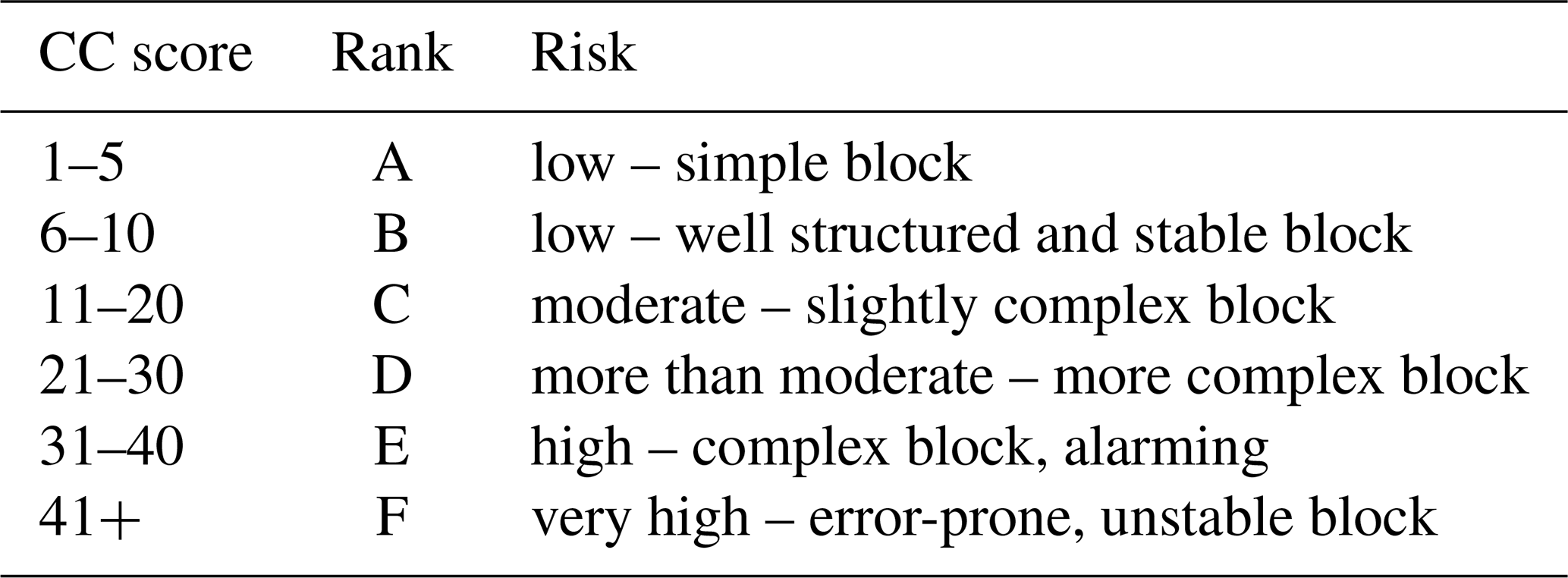
The mean cyclomatic complexity of all code blocks in the new Python code is 5.74 (B); for those blocks with C to F, it is 21 (C). In version 7.0.4, the corresponding numbers are 13 (C) and 31.86 (E), indicating a substantial improvement.
For example, the class ControlFile was improved significantly, as well as the class renamed from EIFlexpart to EcFlexpart. On the other hand, the class method deacc_fluxes became more complex in version 7.1. This is mainly due to two new features, ensemble retrieval and the new disaggregation. Nevertheless, the overall code complexity was reduced.
Another software metric is the maintainability index (MI), where values 0–9 indicate low maintainability, 10–19 medium and 20–100 high maintainability.
The index is calculated for a complete Python file.
Both Python versions have in general highly maintainable Python files except FlexpartTools.py in version 7.0.4 with an MI score of 0.0 and EcFlexpart.py in version 7.1 with an MI score of 10.79.
Additionally, we used a source code quality checker program called pylint (Thénault, 2001) which indicates how well the Python style guide PEP8 (van Rossum et al., 2001) is followed. This tool provides an overall rating index with a maximum value of 10. According to this tool, flex_extract version 7.0.4 has a rating of −8.77 and version 7.1 a rating of 9.09. This shows a massive improvement in following the official style guide.
6.1 Conclusions
This paper describes the software package flex_extract v7.1, which retrieves meteorological fields from the ECMWF IFS model and prepares them for use in the Lagrangian particle dispersion model FLEXPART. The package was initially developed in the 1990s and underwent various developments to adapt to changes in the ECMWF environment and the data set characteristics. In the past two years, ECMWF has introduced considerable changes to its software environment for retrieval, reading and accessing data and has also released new data sets. This necessitated a substantial upgrade of flex_extract to adapt to these changes. Moreover, the user community had new requirements for data retrievals which were considered in this version. In the development process, substantial refactoring was carried out, the number of retrievable data sets was increased, user friendliness was improved, current ECMWF software packages considered, an online documentation was built, and a first set of test cases for future regression testing was created. Furthermore, a recently developed and improved disaggregation method for precipitation fields was implemented as an option.
The number of groups using FLEXPART has grown substantially over the past decade, and with the new opportunity of publicly available reanalysis data sets there will likely be even more users interested in trying out and applying FLEXPART for their research. Alongside this reference paper, the newly established Git repository on the FLEXPART community website https://www.flexpart.eu (last access: 16 October 2020) and the online documentation should assist all these users with up-to-date information about changes, releases of new versions, installation and usage, including a documentation useful for future developers.
6.2 Support
FLEXPART has a community website (https://www.flexpart.eu/, last access: 16 October 2020), where flex_extract as a pre-processor has its own subpage (https://www.flexpart.eu/wiki/FpInputMetEcmwf, last access: 17 August 2019). The website features a ticket system to report issues or submit feature requests. The tickets can be viewed by anyone; to create a ticket, registration (https://www.flexpart.eu/wiki/RegisteredUser, last access: 17 August 2019) is necessary. There is also a mailing list for discussion among FLEXPART and FLEXTRA users and with developers, where questions may be asked or experiences be shared, including pre- and post-processing issues. Announcements for all FLEXPART users, such as new releases, are distributed through the list as well. Future contributions to the code are welcome; for granting permission of write access to the Git repository, communication via email or ticket is necessary.
6.3 Future work
In its current status, the online documentation provides a basic reference. In the future, more examples should be provided, including answers to typical user questions and workarounds for known problems. Information about updates and new releases will also be implemented in this documentation.
It is also intended to provide for the optional retrieval of meteorological fields needed as input (initial and boundary conditions) for the WRF model to support the FLEXPART-WRF community.
The unification of the various three-dimensional fields into a single file shall be removed from the Fortran code as this is a simple task that can be fulfilled more efficiently and transparently with ecCodes command-line tools.
The ERA5 reanalysis has ensemble members stored in the enda stream, but the flux data have a different accumulation period and therefore are not yet retrievable. It is planned to allow the retrieval of these ensemble members in the future. Up to now, it has been possible to set flex_extract to retrieve fields on the reduced Gaussian grid. This should be extended to include the octahedral reduced Gaussian grid.
The hybrid vertical velocity is now stored not only for the operational forecasts but also for the new reanalyses; thus, the need to calculate it is diminishing.
In future versions of flex_extract, calc_etadot will probably only be called if really needs to be calculated, not just for multiplying it with as this can be done with sufficient efficiency in Python.
The flex_extract software package is currently provided as a compressed tar file. In the future, a package shall be made available to be installed as a system package for certain GNU–Linux distributions. In this case, only user-specific data will need to reside in the user directories.
First of all, download the release version from the FLEXPART community website. Alternatively, if Git is installed on the target machine, you may clone the latest version of the master branch from the Git repository on the community website.
Git clone --single-branch --branch master
 https://www.flexpart.eu/gitmob/flex_extract
Currently, flex_extract was only tested for a GNU–Linux environment. The installation process depends on the user group (see Sect. 2.1) and the application mode (see Sect. 3.1). One should first decide for the modes and then follow the compact instructions in the corresponding subsections. Shell scripts and Python code snippets mentioned in the Appendix can be found in the directory Testing/Installation/ after unpacking the tarball. For more details see the instructions in the online documentation.
A1 Registration and licences
Table 6 summarizes which registration is required. Follow the given links from the literature to the registration websites (or footnotes).
A separate licence has to be accepted for each ECMWF public data set, regardless of the user group. For the ERA-Interim and CERA-20C data sets, this can be done at the website for “Available ECMWF Public Datasets” (https://confluence.ecmwf.int/display/WEBAPI/Available+ECMWF+Public+Datasets, last access: 11 November 2019). Log in and follow the licence links on the right side for each data set and accept it. For the ERA5 data set this has to be done at the “Climate Data Store (CDS) website” (https://cds.climate.copernicus.eu/cdsapp#!/search?type=dataset, last access: 11 November 2019). Log in and select, on the left panel, product type “Reanalysis” for finding ERA5 data sets. Then follow any link with ERA5 to the full data set record, click on tab “Download data” and scroll down. There is a section “Terms of use”, where the “Accept terms” button has to be clicked. The licences for member-state users are accepted by the user when receiving a so-called “Token”, which generates new passwords for each log-in.
A2 System prerequisites
Remote mode
ECMWF servers provide all required libraries (see Table 7) via an environment module framework. Flex_extract takes care of loading the right modules at runtime.
Gateway mode
In this mode, access to the ECMWF computing and archiving facilities is enabled through an ECaccess gateway server on a local member-state server. The ECaccess framework is necessary to interactively submit jobs to the ECMWF batch system and to transfer files between ECMWF and local gateway server. As a consequence, a member-state gateway server has to be established (https://confluence.ecmwf.int/display/ECAC/ECaccess+Home, last access: 31 October 2019), and a so-called association (https://confluence.ecmwf.int/download/attachments/45759146/ECaccess.pdf; see page 17 ff. for instructions, last access: 28 October 2019) has to be created to use the ECaccess file transfer service ectrans.
The next step is to create an ECaccess certificate to authorize the file transfers and job submissions. This certificate has to be renewed periodically (every 7 d). The certificate is created by executing the command ecaccess-certificate- create on the command line of the local gateway server, and the user is prompted for the ECMWF member-state user name and a password (generated by a token).
$ ecaccess-certificate-create
Please enter your user-id: example_username
Your passcode: ***
Additional dependencies on the local gateway server are Python3 and the Python packages NumPy and genshi.
Use the package management system of your Linux distribution, which requires admin rights. The installation was tested under GNU–Linux Debian buster and Ubuntu 18.04 Bionic Beaver. The following installation instructions refer to a Debian-based system and use apt-get as package manager; of course, other package managers (e.g. aptitude) or other GNU–Linux distributions can be used as well.
apt-get install python3
apt-get install python3-genshi
apt-get install python3-numpy
Local mode
For the local mode, all software dependencies listed in Sect. 3.2 have to be provided. The installation process is the same for the member-state and public access modes.
Use the package management system of your Linux distribution (requires admin rights) to establish the dependencies if not already available. Note that for the Python version of ecCodes, a version 2.13.0 or higher is necessary.
apt-get install python3
apt-get install python3-eccodes
apt-get install python3-genshi
apt-get install python3-numpy
apt-get install gfortran
apt-get install fftw3-dev
apt-get install libeccodes-dev
apt-get install libemos-dev
As currently the CDS and ECMWF API packages are not available as Debian packages, they need to be installed outside the Debian (e.g. Ubuntu) package management system. The CDS API (cdsapi) is required for ERA5 data and the ECMWF Web API (ecmwf-api-client) for all other public data sets.
The recommended way is to use the Python package management system pip.
apt-get install pip
pip install cdsapi
pip install ecmwf-api-client
Note that if you would like to use Anaconda Python, we recommend you follow the installation instructions of Anaconda Python installation for Linux and then install the ecCodes package from Conda.
conda install conda-forge::python-eccodes
Both user groups have to provide keys with their credentials for the web APIs in their home directory. Therefore, follow these instructions:
-
For ECMWF Web API, go to MARS access website (https://confluence.ecmwf.int//display/WEBAPI/Access+MARS, last access: 20 October 2019) and log in with your credentials. Afterwards, on this site in section “Install ECMWF KEY” the key for the ECMWF Web API should be listed. Please follow the instructions in this section under 1 (save the key in a file
.ecmwfapircin your home directory). -
For CDS API, go to CDS API registration (https://cds.climate.copernicus.eu/api-how-to, last access: 25 October 2019) and register there too. Log in at the cdsapi website and follow the instructions at section “Install the CDS API key” to save your credentials in a
.cdsapircfile in your home directory.
Since a single retrieval run of flex_extract can take a while, it is recommended to do some basic tests for the local access method to identify problems with the web APIs early on. A very simple test retrieval for both web APIs is enough to be sure that everything works. For the ECMWF Web API and as a member-state user, please use the following piece of Python code.
from ecmwfapi import ECMWFService

server = ECMWFService('mars')

server.retrieve({
	'stream'    : "oper",
	'levtype'   : "sfc",
	'param'     : "165.128/166.128/167.128",
	'dataset'   : "interim",
	'step'      : "0",
	'grid'      : "0.75/0.75",
	'time'      : "00/06/12/18",
	'date'      : "2014-07-01/to/2014-07-31",
	'type'      : "an",
	'class'     : "ei",
	'target'    : "download_erainterim_ecmwfapi.grib"
})
For the ECMWF Web API and as a public user, please use the following piece of Python code.
from ecmwfapi import ECMWFDataServer

server = ECMWFDataServer()

server.retrieve({
	'stream'    : "enda",
	'levtype'   : "sfc",
	'param'     : "165.128/166.128/167.128",
	'dataset'   : "cera20c",
	'step'      : "0",
	'grid'      : "1./1.",
	'time'      : "00/06/12/18",
	'date'      : "2000-07-01/to/2000-07-31",
	'type'      : "an",
	'class'     : "ep",
	'target'    : "download_cera20c_ecmwfapi.grib"
})
Extraction of ERA5 data via CDS API might take time as currently, at the time of publication, there is a high demand for ERA5 data. Therefore, as a simple test for the API, just retrieve pressure-level data (even if that is NOT what we need for FLEXPART), as they are stored on disk and do not need to be retrieved from MARS (which is the time-consuming action): please use this piece of Python code (both user groups) to retrieve a small sample of ERA5 pressure levels:
import cdsapi

c = cdsapi.Client()

c.retrieve("reanalysis-era5-pressure-levels",
{
	"variable": "temperature",
	"pressure_level": "1000",
	"product_type": "reanalysis",
	"year": "2008",
	"month": "01",
	"day": "01",
	"time": "12:00",
	"format": "grib"
},
"download_cdsapi.grib")
An example for retrieving ERA5 data from MARS is shown below and can be tested if the code from above worked.
import cdsapi

c = cdsapi.Client()

c.retrieve('reanalysis-era5-complete',
{
	'class'   : 'ea',
	'expver'  : '1',
	'stream'  : 'oper',
	'type'    : 'fc',
	'step'    : '3/to/12/by/3',
	'param'   : '130.128',
	'levtype' : 'ml',
	'levelist': '135/to/137',
	'date'    : '2013-01-01',
	'time'    : '06/18',
	'area'    : '50/-5/40/5',
	'grid'    : '1.0/1.0',
	'format'  : 'grib',
}, 'download_era5_cdsapi.grib')
A3 Building flex_extract
Remote mode
First, log in on one of the ECMWF servers, such as ecgate or cca/ccb. Second, copy the tar file to the server, untar the flex_extract release tarball and switch into the flex_extract root directory.
scp <localuser>@<localmachine.tld>:</path/to/tarfile> $HOME
cd $HOME
tar xvf flex_extract_vX.X.tar.gz
cd flex_extract_vX.X
Substitute the <localuser> and <localmachine.tld> placeholders with your local user name and the IP name or address of your local machine.
Finally, adapt the parameters (described in Tables 11 and 9) in the setup.sh script and execute it.
Flex_extract, uses the email address connected to the user account to notify the user about successful or failed installation.
Gateway mode
The actual execution of flex_extract with retrieval and preparation of the data will be run on ECMWF servers. The only difference is the preparation of the job script, which is done on the local gateway server and sent to ECMWF servers by the ECaccess services.
Unpack the release tarball and switch into its directory. Substitute X.X with the actual release version number.
tar xvf flex_extract_vX.X.tar.gz
cd flex_extract_vX.X
Afterwards, prepare the setup.sh script by configuring its parameters (described in Table 11 and 9) and execute it. The makefile has to be selected according to the selection of the target, e.g. ecgate or cca/ccb servers. In this mode the DESTINATION and GATEWAY parameters have to be set to be able to use the ectrans service.
A configuration job script is then sent to the ECMWF batch queue and flex_extract uses the email address connected to the user account to notify the user about successful or failed installation.
Local mode
Since flex_extract compiles the Fortran program calc_etadot during the installation process, a corresponding makefile has to be provided. Flex_extract comes with a prepared makefile for the gfortran (https://gcc.gnu.org/fortran/, last access: 16 October 2020) compiler. The makefile assumes that ecCodes and EMOSLIB are installed as distribution packages.
It is necessary to adapt the two parameters ECCODES_INCLUDE_DIR and ECCODES_LIB in these makefiles if something other than standard paths is used.
Therefore, if needed, prepare the Fortran makefile for your environment by starting from the makefile makefile_fast provided and edit the paths to point to the ecCodes library on your local machine. It can be found at flex_extract_vX.X/Source/Fortran, where vX.X should be substituted with the current version number.
Finally, adapt the command-line parameters (described in Tables 9 and 11) in the setup.sh script in the root directory of flex_extract and execute it.
A4 Installation test
The most common errors in applying flex_extract arise from wrong installation and settings regarding the libraries for the Fortran program. Therefore it is useful to do a simple test with a prepared minimal data set. The following instructions have to be executed on the local system for the local mode and on the ECMWF servers in the remote and gateway mode.
From the flex_extract root directory, switch into the Testing/Installation/Calc_etadot/ directory and execute the Fortran program by
cd Testing/Installation/Calc_etadot
# execute the Fortran program
../../../Source/Fortran/calc_etadot
The installation was successful if you obtain the following on standard output.
STATISTICS:          98842.4598  98709.7359   5120.5385
STOP SUCCESSFULLY FINISHED calc_etadot: CONGRATULATIONS
Note that on ECMWF servers the flex_extract root directory is placed in the $HOME directory.
Flex_extract is a command-line tool which can be started by executing the submit.py script in the Python source directory or more preferably with an upstream shell script run.sh which calls the submit.py script with its corresponding command-line arguments.
Therefore, the user should navigate to the Run directory, where the shell script is located.
cd <path-to-flex_extract_vX.X>/Run
with X.X as the placeholder for the version number.
This directory contains all information necessary to run flex_extract. The only files which might need modifications by the user are the run.sh script and the selected CONTROL file within the Control directory. This directory contains a sample set of the current range of possible data set retrievals.
This section describes the basic steps to start a flex_extract retrieval within the different modes based on an example. More details about the usage can be found in Sect. 4 and in the online documentation, especially specifics of different data sets and CONTROL file parameters.
For the first data retrieval it is recommended to use one of the example CONTROL files stored in the Control directory to avoid unnecessary problems. We recommend to extract CERA-20C data since they are usually not highly demanded and guarantee quick processing for the best testing experience. In the following, we will provide step-by-step instructions for all application modes to retrieve a single day (8 September 2000) from the CERA-20C data set with 3-hourly temporal resolution and a small domain over Europe with 1∘ resolution, using CONTROL_CERA[.public].
Remote and gateway modes
For member-state users it is recommended to use the remote or gateway mode, especially for more demanding tasks, to retrieve and post-process data on ECMWF machines and to transfer only the final output files to the local host.
The only difference between both modes is the location where flex_extract will be started from. In the remote mode we work directly on the ECMWF server; therefore log in to the ECMWF server of your choice and switch to the Run directory as shown above. Remember, at ECMWF servers flex_extract is always installed in the $HOME directory. Within the gateway mode, only a switch into the Run directory of flex_extract on the gateway server is necessary.
Otherwise, the rest of the working steps are the same in both modes. Now, open the run.sh script and modify the parameter block marked in the file as shown below. The parameters are described in Table 12.
# -----------------------------------------
# AVAILABLE COMMANDLINE ARGUMENTS TO SET
#
# THE USER HAS TO SPECIFY THESE PARAMETERS:

QUEUE='ecgate'
START_DATE=None
END_DATE=None
DATE_CHUNK=None
JOB_CHUNK=3
BASETIME=None
STEP=None
LEVELIST=None
AREA=None
INPUTDIR=None
OUTPUTDIR=None
PP_ID=None
JOB_TEMPLATE='submitscript.template'
CONTROLFILE='CONTROL_CERA'
DEBUG=0
REQUEST=2
PUBLIC=0
This would retrieve CERA-20C data on the ECMWF server ecgate. For the ECMWF cca/ccb servers, the parameter QUEUE has to be adapted. Since the ectrans parameter in the CONTROL_CERA file is set to 1, the resulting output files will be transferred to the local gateway into the path stored in the destination, provided that the destination was correctly set up.
Please note that success of the submission of the ectrans command does not guarantee that the file transfer will succeed. It means only that the output file has been successfully submitted to the ectrans queueing system. One still has to check manually in the local directories or with ECaccess tools whether the files reached their final destination. The parameters listed in the run.sh script would overwrite existing settings from the CONTROL file.
Starting the retrieval process will be done by executing the script by ./run.sh. Flex_extract will print some information about the job on standard output. If there is no error in the submission to the ECMWF server, a message like this will be shown:
---- On-demand mode! ----
The job id is: 10627807
You should get an email per job with
    subject flex.hostname.pid
FLEX_EXTRACT JOB SCRIPT IS SUBMITTED!
Once submitted, the job status can be checked by using the command ecaccess-job-list. At the end of the job, the user should receive an email with a detailed protocol of what was done and if the job was successful.
In the case that the job failed, the subject will contain the keyword ERROR! and the job name. Then, the user can check the email or on ECMWF servers in the $SCRATCH directory for debugging information.
In the $SCRATCH directory on ecgate it is recommended to list the content with ls -rthl to list the most recent logs and temporary retrieval directories (usually extractXXXXX, where XXXXX is the process ID). Under extractXXXXX a copy of the CONTROL file is stored under the name CONTROL, the protocol is stored in the file prot, and the temporary files as well as the resulting files are stored in a directory work. The original name of the CONTROL file can be found within this new file under parameter controlfile.
If the job was submitted to the high-performance computer (HPC) (QUEUE is cca or ccb) you may login to the HPC and look in the directory /scratch/ms/ECGID/ECUID/.ecaccess_do_not_remove for job logs. The working directories are deleted after job failure and thus normally cannot be accessed.
If the resulting files cannot be found in the destination path of the local gateway server, it can be checked whether the files are still to be transferred to the local gateway server by using the command ecaccess-ectrans-list.
After this test retrieval was successful, feel free to try changing the CONTROL file parameters described in Table 8 by selecting other CONTROL files. Please keep in mind the considerations of application in Sect. 4.
Local mode
Since this mode can be used by member-state and public users, we show an example for both user groups. Open the run_local.sh file and adapt the parameter block marked in the file as shown for the corresponding user group. The parameters are described in Table 12.
Take this setting as a member-state user:
# -----------------------------------------
# AVAILABLE COMMANDLINE ARGUMENTS TO SET
#
# THE USER HAS TO SPECIFY THESE PARAMETERs:
#

QUEUE=''
START_DATE=None
END_DATE=None
DATE_CHUNK=None
JOB_CHUNK=None
BASETIME=None
STEP=None
LEVELIST=None
AREA=None
INPUTDIR='./Workspace/CERA'
OUTPUTDIR=None
PP_ID=None
JOB_TEMPLATE=''
CONTROLFILE='CONTROL_CERA'
DEBUG=0
REQUEST=0
PUBLIC=0
and take this setting as a public user:
# -----------------------------------------
# AVAILABLE COMMANDLINE ARGUMENTS TO SET
#
# THE USER HAS TO SPECIFY THESE PARAMETERs:
#

QUEUE=''
START_DATE=None
END_DATE=None
DATE_CHUNK=None
JOB_CHUNK=None
BASETIME=None
STEP=None
LEVELIST=None
AREA=None
INPUTDIR='./Workspace/CERApublic'
OUTPUTDIR=None
PP_ID=None
JOB_TEMPLATE=''
CONTROLFILE='CONTROL_CERA.public'
DEBUG=0
REQUEST=0
PUBLIC=1
The working location for this retrieval is set by the INPUTDIR parameter and will be the Workspace/CERA* directory within the current Run directory. It is also the output directory since OUTPUTDIR was not set. This can be changed to whatever path is preferred. The parameters listed in run_local.sh would overwrite existing settings in the CONTROL file.
Starting the retrieval process will be done by executing the script by ./run_local.sh.
While a job submission on the local host is convenient and easy to monitor (on standard output), there are a few caveats with this option.
There is a maximum size of 20 GB for single retrievals via ECMWF Web API. Normally this is not a problem, but for global fields with T1279 resolution and hourly time steps the limit may already apply.
If the retrieved MARS files are large but the resulting files are relatively small (small local domain, but large time period), then the retrieval to the local host may be inefficient since all data must be transferred via the Internet. This scenario applies most notably if ETADOT has to be calculated via the continuity equation as this requires global fields even if the domain is local and small. In this case, job submission via ecgate might be a better choice. It really depends on the patterns used and also on the speed of the Internet.
After this test retrieval is successful, feel free to try changing the CONTROL file parameters described in Table 8 and selecting other CONTROL files. Please keep in mind the considerations of application in Sect. 4.
Flex_extract is a code package consisting of Python scripts, shell scripts and a Fortran program; it is open software distributed under a Creative Commons (CC-BY-4.0) licence. The latest version of the code (currently 7.1.2) is available through the flex_extract project web page (https://www.flexpart.eu/wiki/FpInputMetEcmwf, last access: 9 July 2020), which is part of the FLEXPART community website and contains links to the tarball and the Git repository. The online documentation is also hosted there (https://www.flexpart.eu/flex_extract/, last access: 9 July 2020).
The exact version corresponding to this manuscript is archived on Phaidra (https://phaidra.univie.ac.at/o:1097971, last access: 16 October 2020), the permanent secure storage of the University of Vienna.
The software package comes with a number of test cases which should be used by developers in the future. Some tests need additional reference data which have to be downloaded separately from the project website.
The following open-source libraries have to be available in addition to the libraries mentioned in the installation section in order to run the flex_extract test cases: numpy/scipy (Walt et al., 2011), pandas (McKinney, 2010), xarray (Hoyer and Hamman, 2017), pytest (Krekel, 2019) and mock (Foord and the mock team, 2019).
For the generation of the online documentation, the Python package sphinx (Brandl, 2019) is required; for the documentation of the Fortran code, FORD (http://fortranwiki.org/fortran/show/FORD, last access: 20 December 2019) is required.
The current version 7.1.2 of flex_extract was developed under GNU–Linux and was tested only on this platform. Application under other operating systems may be possible but without support from the developers.
The supplement related to this article is available online at: https://doi.org/10.5194/gmd-13-5277-2020-supplement.
AT revised the complete software package (except for the Fortran part) and applied the necessary changes to keep it up to date with the ECMWF software environment. She coordinated and added new implementations and guided the evaluation. She wrote the online documentation as well as most of the manuscript. LH is the original author of the software package and provided the first implementation for the use of the ECMWF Web API and the retrieval of ensemble members. He participated in writing introductory and history parts as well as giving feedback on all other parts. PS revised the Fortran code and provided the Fortran code documentation and test cases, and wrote the respective section of the manuscript. She also gave feedback on all other parts and contributed to editing the final manuscript version.
The authors declare that they have no conflict of interest.
Over the years, the development of flex_extract was partly funded by the CTBTO. We thank the ZAMG for providing access to the ECMWF MARS archive and the hosting of the community website. We would also like to thank the ECMWF user support for their assistance in converging the software environment to the current state and for their many publicly available code examples for working with GRIB files. Additionally, we thank Anne Fouilloux for an initial version of the Python routines. Moreover, we thank the users for their feedback and questions which made it possible to make progress in user friendliness, eliminate bugs and react to requirements.
Open-access funding was provided by the University of Vienna.
This paper was edited by Paul Ullrich and reviewed by three anonymous referees.
Beizer, B.: Software Testing Techniques, 2nd edn., Van Nostrand Reinhold, 115 Fifth Avenue, New York, NY 10003, 550 pp., ISBN 0-442-20672-0, 1990. a, b, c
Berrisford, P., Dee, D., Poli, P., Brugge, R., Fielding, M., Fuentes, M., Kållberg, P., Kobayashi, S., Uppala, S., and Simmons, A.: The ERA-Interim archive Version 2.0, ERA Report Series, Vol. 1, available at: https://www.ecmwf.int/node/8174 (last access: 16 October 2020), 2011. a, b, c
Brandl, G.: Sphinx - Python Documentation Generator, available at: http://www.sphinx-doc.org/en/master/, last access: 12 December 2019. a
Buizza, R., Richardson, D. S., and Palmer, T. N.: Benefits of increased resolution in the ECMWF ensemble system and comparison with poor-man's ensembles, Q. J. Roy. Meteor. Soc., 129, 1269–1288, https://doi.org/10.1256/qj.02.92, 2003. a
Copernicus: How to use the CDS API, available at: https://cds.climate.copernicus.eu/api-how-to, last access: 3 September 2019. a
ECMWF: ERA-Interim: What is the spatial reference, available at: https://confluence.ecmwf.int/display/CKB/ERA-Interim%3A+What+is+the+spatial+reference (last access: 26 August 2019), 2016a. a
ECMWF: ERA5: What is the spatial reference, available at: https://confluence.ecmwf.int/display/CKB/ERA5%3A+What+is+the+spatial+reference (last access: 26 August 2019), 2016b. a
ECMWF: OpenIFS: Horizontal Resolution Configurations, available at: https://confluence.ecmwf.int/display/OIFS/4.2+OpenIFS%3A+Horizontal+Resolution+Configurations (last access: 8 June 2020), 2017. a
ECMWF: ECMWF, available at: https://www.ecmwf.int, last access: 5 August 2019a. a
ECMWF: MARS User Documentation, available at: https://software.ecmwf.int/wiki/display/UDOC/MARS+user+documentation, last access: 5 August 2019b. a, b
ECMWF: Forecasting system upgrade set to improve global weather forecasts, available at: https://www.ecmwf.int/en/about/media-centre/news/2019/forecasting-system-upgrade-set-improve-global-weather-forecasts, last access: 24 August 2019c. a
ECMWF: Data spatial coordinate systems, available at: https://www.ecmwf.int/en/forecasts/documentation-and-support/data-spatial-coordinate-systems (last access: 26 August 2019), 2019d. a
ECMWF: MARS Catalogue, available at: https://apps.ecmwf.int/mars-catalogue/, last access: 27 August 2019e. a, b, c, d, e, f
ECMWF: Changes in ECMWF model, available at: https://www.ecmwf.int/en/forecasts/documentation-and-support/changes-ecmwf-model, last access: 27 August 2019f. a
ECMWF: IFS Documentation, available at: https://www.ecmwf.int/en/publications/ifs-documentation, last access: 26 August 2019g. a
ECMWF: ERA5 data documentation, available at: https://confluence.ecmwf.int/display/CKB/ERA5+data+documentation, last access: 27 August 2019h. a
ECMWF: Parameter database, available at: https://apps.ecmwf.int/codes/grib/param-db, last access: 28 August 2019i. a, b
ECMWF: Ecaccess concepts, available at: https://confluence.ecmwf.int/display/ECAC/Ecaccess+concepts, last access: 28 August 2019j. a, b
ECMWF: ECMWF Web API Home, available at: https://confluence.ecmwf.int/display/WEBAPI/ECMWF+Web+API+Home, last access: 3 September 2019k. a
ECMWF: What are the changes from ERA-Interim to ERA5?, available at: https://confluence.ecmwf.int/pages/viewpage.action?pageId=74764925, last access: 16 October 2020l. a
ECMWF: Tutorials, available at: https://confluence.ecmwf.int/display/METV/Tutorials, last access: 18 December 2019m. a
Foord, M. and the mock team: Mock object library, available at: https://mock.readthedocs.io/en/latest/, last access: 12 December 2019. a
Hersbach, H., Bell, B., Berrisford, P., Hirahara, S., Horányi, A., Munoz-Sabater, J., Nicolas, J., Peubey, C., Radu, R., Schepers, D., Simmons, A., Soci, C., Abdalla, S., Abellan, X., Balsamo, G., Bechtold, P., Biavati, G., Bidlot, J., Bonavita, M., Chiara, G. D., Dahlgren, P., Dee, D., Diamantakis, M., Dragani, R., Flemming, J., Forbes, R., Fuentes, M., Geer, A., Haimberger, L., Healy, S., Hogan, R. J., Hólm, E., Janisková, M., Keeley, S., Laloyaux, P., Lopez, P., Radnoti, G., de Rosnay, P., Rozum, I., Vamborg, F., Villaume, S., and Thépaut, J.-N.: The ERA5 Global Reanalysis, Quart. J. Roy. Met. Soc., 146, 1999–2049, https://doi.org/10.1002/qj.3803, 2020. a, b
Hittmeir, S., Philipp, A., and Seibert, P.: A conservative reconstruction scheme for the interpolation of extensive quantities in the Lagrangian particle dispersion model FLEXPART, Geosci. Model Dev., 11, 2503–2523, https://doi.org/10.5194/gmd-11-2503-2018, 2018. a, b, c, d, e, f, g
Hoyer, S. and Hamman, J.: xarray: N-D labeled arrays and datasets in Python, Journal of Open Research Software, 5, https://doi.org/10.5334/jors.148, 2017. a
Krekel, H.: pytest Documentation, available at: https://buildmedia.readthedocs.org/media/pdf/pytest/latest/pytest.pdf, last access: 12 December 2019. a
Lacchia, M.: radon 4.0.0 – Project description, available at: https://pypi.org/project/radon/, last access: 12 December 2019. a, b, c
Laloyaux, P., Balmaseda, M., Dee, D., Mogensen, K., and Janssen, P.: A coupled data assimilation system for climate reanalysis, Q. J. Roy. Meteor. Soc., 142, 65–78, https://doi.org/10.1002/qj.2629, 2016. a, b
Laloyaux, P., de Boisseson, E., Balmaseda, M., Bidlot, J.-R., Broennimann, S., Buizza, R., Dalhgren, P., Dee, D., Haimberger, L., Hersbach, H., Kosaka, Y., Martin, M., Poli, P., Rayner, N., Rustemeier, E., and Schepers, D.: CERA-20C: A Coupled Reanalysis of the Twentieth Century, J Adv. Model. Earth Sy., 10, 1172–1195, https://doi.org/10.1029/2018MS001273, 2018. a
McKinney, W.: Data Structures for Statistical Computing in Python, in: Proceedings of the 9th Python in Science Conference, Austin, Texas, 28 June–3 July 2010, edited by: van der Walt, S. and Millman, J., 51–56, https://doi.org/10.25080/Majora-92bf1922-00a, 2010. a
Palmer, T. N., Barkmeijer, J., Buizza, R., and Petroliagis, T.: The ECMWF Ensemble Prediction System, Meteorol. Appl., 4, 301–304, https://doi.org/10.1017/S1350482797000649, 1997. a
Pisso, I., Sollum, E., Grythe, H., Kristiansen, N. I., Cassiani, M., Eckhardt, S., Arnold, D., Morton, D., Thompson, R. L., Groot Zwaaftink, C. D., Evangeliou, N., Sodemann, H., Haimberger, L., Henne, S., Brunner, D., Burkhart, J. F., Fouilloux, A., Brioude, J., Philipp, A., Seibert, P., and Stohl, A.: The Lagrangian particle dispersion model FLEXPART version 10.4, Geosci. Model Dev., 12, 4955–4997, https://doi.org/10.5194/gmd-12-4955-2019, 2019. a, b, c, d
Ritchie, H., Temperton, C., Simmons, A., Hortal, M., Davies, T., Dent, D., and Hamrud, M.: Implementation of the Semi–Lagrangian Method in a High–Resolution Version of the ECMWF Forecast Model, Mon. Weather Rev., 123, 489–514, https://doi.org/10.1175/1520-0493(1995)123<0489:IOTSLM>2.0.CO;2, 1995. a
Simmons, A. J. and Burridge, D. M.: An Energy and Angular–Momentum Conserving Vertical Finite-Difference Scheme and Hybrid Vertical Coordinates, Mon. Weather Rev., 109, 758–766, https://doi.org/10.1175/1520-0493(1981)109<0758:AEAAMC>2.0.CO;2, 1981. a, b
Sneed, H. M., Seidl, R., and Baumgartner, M.: Software in Zahlen, Hanser, Munich, ISBN 978-3-446-42175-2, 357 pp., 2010. a
Spillner, Andreas; Linz, T.: Basiswissen Softwaretest, 5th edn., dpunkt, Heidelberg, ISBN 978-3-86490-024-2, 290 pp., 2012. a
Stohl, A. and Seibert, P.: Accuracy of trajectories as determined from the conservation of meteorological tracers, Q. J. Roy. Meteor. Soc., 125, 1465–1584, https://doi.org/10.1002/qj.49712454907, 1998. a, b, c
Stohl, A., Wotawa, G., Seibert, P., and Kromp-Kolb, H.: Interpolation errors in wind fields as a function of spatial and temporal resolution and their impact on different types of kinematic trajectories, J. Appl. Meteorol., 34, 2149–2165, https://doi.org/10.1175/1520-0450(1995)034<2149:IEIWFA>2.0.CO;2, 1995. a, b, c
Stohl, A., Hittenberger, M., and Wotawa, G.: Validation of the Lagrangian particle dispersion model FLEXPART against large-scale tracer experiment data, Atmos. Environ., 32, 4245–4264, https://doi.org/10.1016/S1352-2310(98)00184-8, 1998. a, b, c
Stohl, A., Haimberger, L., Scheele, M., and Wernli, H.: An intercomparison of results from three trajectory models, Meteorol. Appl., 8, 127–135, https://doi.org/10.1017/S1350482701002018, 2001. a
Stohl, A., Forster, C., Frank, A., Seibert, P., and Wotawa, G.: Technical note: The Lagrangian particle dispersion model FLEXPART version 6.2, Atmos. Chem. Phys., 5, 2461–2474, https://doi.org/10.5194/acp-5-2461-2005, 2005 a, b, c
Thénault, S.: Pylint, available at: https://www.pylint.org/ (last access: 11 December 2019), 2001. a
van Rossum, G., Warsaw, B., and Coghlan, N.: PEP 8 – Style Guide for Python Code, available at: https://www.python.org/dev/peps/pep-0008/ (last access: 16 October 2020), 2001. a
Walt, S. v. d., Colbert, S. C., and Varoquaux, G.: The NumPy array: A structure for efficient numerical computation, Comput. Sci. Eng., 13, 22–30, https://doi.org/10.1109/MCSE.2011.37, 2011. a
Wolff, E.: Continuous Delivery: Der pragmatische Einstieg, Dpunkt Verlag, Heidelberg, ISBN 978-3-86490-208-6, 282 pp., 2014. a
Wotawa, G., Stohl, A., and Neininger, B.: The urban plume of Vienna: comparisons between aircraft measurements and photochemical model results, Atmos. Environ., 32, 2479–2489, https://doi.org/10.1016/S1352-2310(98)00021-1, 1998. a
- Abstract
- Introduction
- ECMWF data
- Software description and methods
- Considerations for application
- Quality assurance
- Final remarks and outlook
- Appendix A: Installation instructions
- Appendix B: Usage instructions
- Code and data availability
- Author contributions
- Competing interests
- Acknowledgements
- Financial support
- Review statement
- References
- Supplement