the Creative Commons Attribution 4.0 License.
the Creative Commons Attribution 4.0 License.
 | 02 Nov 2020
Development of a submerged aquatic vegetation growth model in the Coupled Ocean–Atmosphere–Wave–Sediment Transport (COAWST v3.4) model
Tarandeep S. Kalra
Neil K. Ganju
Jeremy M. Testa
The coupled biophysical interactions between submerged aquatic vegetation (SAV), hydrodynamics (currents and waves), sediment dynamics, and nutrient cycling have long been of interest in estuarine environments. Recent observational studies have addressed feedbacks between SAV meadows and their role in modifying current velocity, sedimentation, and nutrient cycling. To represent these dynamic processes in a numerical model, the presence of SAV and its effect on hydrodynamics (currents and waves) and sediment dynamics was incorporated into the open-source Coupled Ocean–Atmosphere–Wave–Sediment Transport (COAWST) model. In this study, we extend the COAWST modeling framework to account for dynamic changes of SAV and associated epiphyte biomass. Modeled SAV biomass is represented as a function of temperature, light, and nutrient availability. The modeled SAV community exchanges nutrients, detritus, dissolved inorganic carbon, and dissolved oxygen with the water-column biogeochemistry model. The dynamic simulation of SAV biomass allows the plants to both respond to and cause changes in the water column and sediment bed properties, hydrodynamics, and sediment transport (i.e., a two-way feedback). We demonstrate the behavior of these modeled processes through application to an idealized domain and then apply the model to a eutrophic harbor where SAV dieback is a result of anthropogenic nitrate loading and eutrophication. These cases demonstrate an advance in the deterministic modeling of coupled biophysical processes and will further our understanding of future ecosystem change.
- Article
(3106 KB) - Full-text XML
- BibTeX
- EndNote


Submerged aquatic vegetation (SAV), or seagrass, includes rooted vascular plants that inhabit sediments of estuaries and coastal waters, with a wide global distribution. SAV involves important primary producers in shallow environments and provides a habitat for a number of aquatic organisms; it can slow water velocities and dampen wave energy to trap particulate material (Carr et al., 2010), as well as alter biogeochemical cycles through oxygenation of sediments (Larkum et al., 2006). The positive impact of ecosystem services provided by SAV presence has been well studied (Hemminga and Duarte, 2000; Nixon et al., 2001; Terrados and Borum, 2004; McGlathery et al., 2007; Hayn et al., 2014). The growth of SAV is dependent upon light availability at the leaf surface, which is a function of light attenuation in the water column and the biomass of epiphytic algae growing on SAV stems. During the last several decades, the loss of SAV has accelerated due to anthropogenic pressures (Kennish et al., 2016) or natural causes such as storms (Hamberg et al., 2017). One of the dominant factors of SAV loss is eutrophication through nutrient loading, exemplified by increased phytoplankton growth and epiphytic growth on vegetation. This results in a reduction of light availability (Burkholder et al., 2007), causing a loss of SAV habitat (Cabello-Pasini et al., 2003; Short and Neckles, 1999).
The complex interactions between light availability, nutrient loading, SAV dynamics, hydrodynamics, and sediment transport can be investigated using numerical modeling tools. Few modeling efforts have attempted to couple the effects of hydrodynamics and light availability to model the growth of SAV. Everett et al. (2007) and Hipsey and Hamilton (2008) coupled the effects of chlorophyll and water to account for SAV variability, while Bissett et al. (1999a, b) used spectral underwater irradiance to model the light availability required for SAV growth. Carr et al. (2012a, b) developed a one-dimensional coupled hydrodynamics, sediment, and vegetation growth dynamics model. The model solved for vertical 1-D dynamics of SAV growth through a change in biomass that depended on water temperature, irradiance, and seagrass properties. Ganju et al. (2012) used a three-dimensional circulation model (Regional Ocean Modeling System; ROMS) coupled to a nutrient–phytoplankton–zooplankton–detritus (NPZD) eutrophication (water-column biogeochemistry model) developed by Fennel et al. (2006) and integrated the spectral light attenuation formulation (bio-optical model) provided by Gallegos et al. (2011). These models were linked to a benthic seagrass model to calculate seagrass distribution (Zimmerman, 2003) and applied on the temperate estuary of West Falmouth Harbor (del Barrio et al., 2014). While the model was able to capture the loss of SAV due to insufficient light, it did not include interactions with epiphytes or exchanges with water-column nutrients and gas pools. The hydrodynamic feedbacks (changes in currents and waves) and morphodynamic changes (sediment distribution) due to presence of SAV were also ignored. While these dynamic processes have significant implications for coastal ecosystem resilience, numerical models that allow for the two-way feedbacks between hydrodynamics, sediment transport, and SAV growth and nutrient cycling have generally been lacking.
Recently, Beudin et al. (2017) implemented the physical effects of SAV in a vertically varying water column through momentum extraction and vertical mixing as well as accounting for wave dissipation due to vegetation. These processes were implemented within the open-source Coupled Ocean–Atmosphere–Wave–Sediment Transport (COAWST) modeling system that couples the hydrodynamic model (ROMS), the wave model (Simulating WAves Nearshore; SWAN), and the Community Sediment-Transport Modeling System (CSTMS) (Warner et al., 2010). Through this effort, the COAWST framework accounted for the coupled seagrass–hydrodynamics interactions. The model reproduced the turbulent shear stress across the canopy interface and peaked at the top of the canopy similar to the observations of Ghisalberti and Nepf (2004, 2006). The presence of a seagrass patch led to a reduced shear-scale turbulence within the canopy and enhanced wake-scale generated turbulence. For more details on the impact of seagrass on hydrodynamics, readers are referred to Beudin et al. (2017). The inclusion of the physical effects of SAV on flow and sediment dynamics (Beudin et al., 2017) in COAWST allows us to develop a framework that results in dynamic growth of SAV using the temperature, nutrient loading, and light availability in the water column. Therefore, in this work, we implement a SAV growth model that dynamically changes the SAV properties (stem density and height). The growth of SAV is modeled as biomass which includes the aboveground biomass (stems and shoots), belowground (roots and rhizomes) biomass, and epiphyte biomass. Individual biomass equations described in the implementation of SAV growth model (Sect. 2.2) are based on previous SAV biomass models (primarily Madden and Kemp, 1996), some of which have been previously implemented to simulate growth conditions for SAV in three-dimensional numerical model simulations (e.g., Cerco and Moore, 2001). The change in biomass leads to a spatial and temporal variation of SAV density and height. With the inclusion of the SAV growth model, SAV can experience growth or dieback while contributing and sequestering nutrients from the water column (modifying the biological environment) and subsequently affect the hydrodynamics and sediment transport (modifying the physical environment). Conversely, a change in the physical environment, for instance, the amount of sediment in the water column, can decrease light availability and cause SAV dieback, leading to reduced wave attenuation, increased sediment resuspension, and a further decrease of light availability.
We demonstrate the two-way biophysical coupling framework as follows: the SAV growth model and integration into COAWST are discussed in Sect. 2; in Sect. 3, the model setup for the idealized domain and a realistic simulation of West Falmouth Harbor, Massachusetts, are described; in Sect. 4, we present the results from the two model configurations along with a discussion of limitations of the current modeling work; and in Sect. 5, we summarize our work and outline areas of future research.
2.1 Inclusion of SAV effect on flow and sediment dynamics in the numerical model
Beudin et al. (2017) implemented the parameterizations that accounted for the presence of SAV within a coupled hydrodynamic and wave model within the open-source COAWST numerical modeling system (Warner et al., 2008). The COAWST framework utilizes ROMS for hydrodynamics with a wave model (SWAN) via the Model Coupling Toolkit (MCT), generating a single executable program (Warner et al., 2008). ROMS is a three-dimensional, free surface, finite-difference, terrain-following model that solves the Reynolds-averaged Navier–Stokes (RANS) equations using the hydrostatic and Boussinesq assumptions (Haidvogel et al., 2008). The transport of turbulent kinetic energy and generic length scale is computed with a generic (GLS) two-equation turbulence model. SWAN is a third-generation spectral wave model based on the action balance equation (Booij et al., 1999). In ROMS, the presence of SAV extracts momentum, adds wave-induced streaming, and generates turbulence dissipation. Similarly, the wave dissipation due to vegetation modifies the source term of the action balance equation in SWAN. All of these subgrid-scale parameterizations account for changes due to vegetation in the water column extending from the bottom layer to the height of the vegetation. SWAN only accounts for wave dissipation due to vegetation at the bottom layer. The coupling between the two models occurs with an exchange of water level and depth-averaged velocities from ROMS to SWAN and wave fields from SWAN to ROMS after a desired number of time steps. The vegetation properties are separately input in the two models at the beginning of the simulations. Through these changes, the SAV can affect the bottom stress calculations that determine the resuspension and transport of sediment, providing a feedback loop between SAV–sediment dynamics–hydrodynamics and wave dynamics. To account for sediment dynamics, CSTMS (Warner et al., 2010) is used to track the transport of suspended-sediment and bed load transport under the action of current and wave–current forcing. The model can represent an unlimited number of user-defined sediment classes.
2.2 SAV growth model
The SAV growth model is primarily based upon a previous growth model developed and implemented in Chesapeake Bay by Madden and Kemp (1996). The model simulates the temporal dynamics of aboveground biomass (AGB) that consists of stems or shoots, and the belowground biomass (BGB) that consists of roots or rhizomes. In addition to AGB and BGB, epiphytic algal biomass (EPB) is simulated to account for reductions in light availability to plant leaves due to shading of SAV leaves by epiphytes under high nutrient loading conditions. AGB, BGB, and EPB are simulated as total biomass per unit area, with nitrogen as the currency for biomass. Changes in AGB and BGB pools are simulated as a function of primary production and respiration, mortality (e.g., grazing), and nitrogen exchange through the seasonal translocation of nitrogen between roots and shoots. EPB is modeled as a function of primary production, respiration, and mortality.
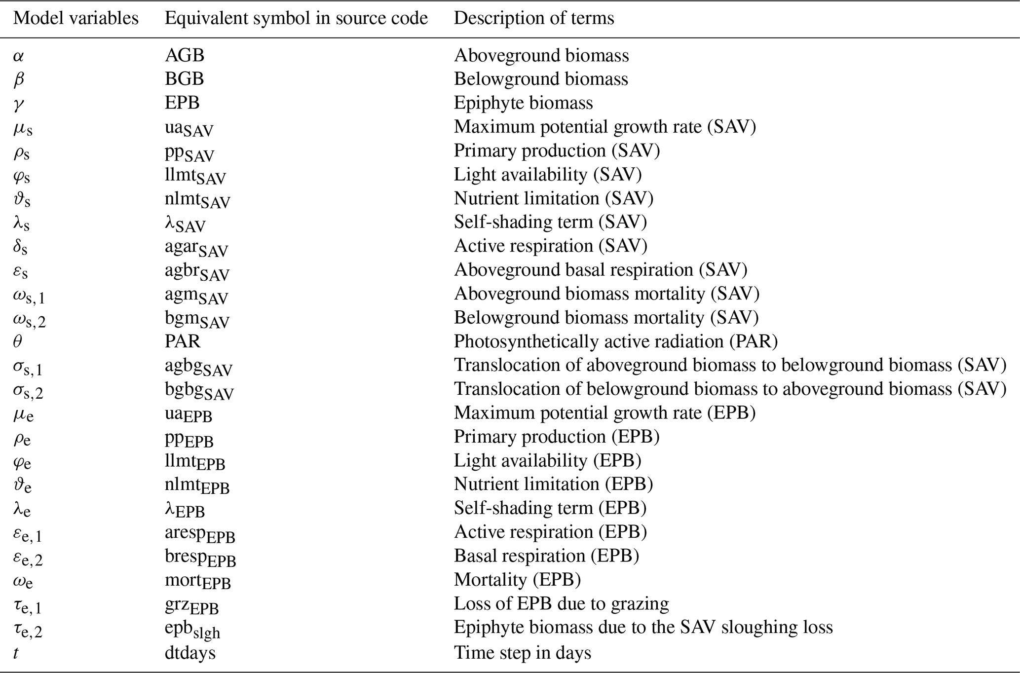
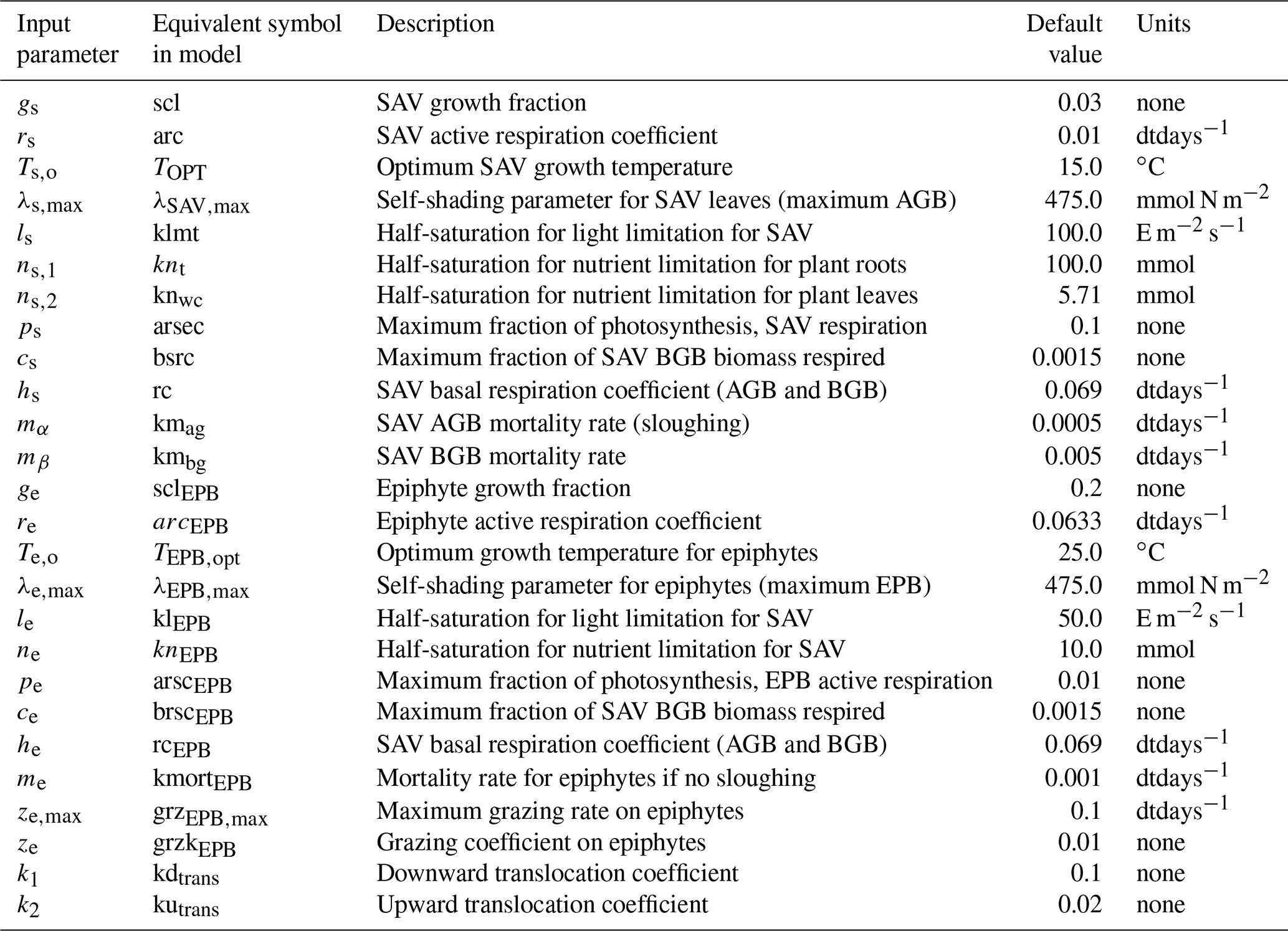
Table 2SAV growth model input parameter descriptions and their values.
The remaining section describes the source terms that calculate the evolution of AGB, BGB, and EPB, denoted by α, β, and γ, respectively. Tables 1 and 2 describe model variables and input parameters along with their equivalent symbols used in the source code.
2.2.1 Primary production (ρs)
The primary production of α depends on the maximum potential growth rate (μs) and downward deviations from this maximal rate resulting from light (φs) and nutrient (ϑs) availability as
The maximum potential growth (μs) can be described as
where λs is a self-shading parameter that accounts for crowding and self-shading within the SAV canopy, gs accounts for SAV's maximum growth fraction, rs is the active SAV respiration coefficient, T is the temperature in the water column, and To is the user-defined optimum temperature that allows for species-specific sensitivities to temperature. The self-shading parameter, λs, used in Eq. (3) is calculated by setting a maximum aerial biomass of SAV (Madden and Kemp, 1996), thereby making growth rates density dependent, and is defined as
where α is the aboveground SAV biomass and λs,max accounts for the maximal SAV biomass.
The availability of photosynthetically active radiation (PAR) represented by mathematical symbol θ for SAV leaves in the bottom cell is simulated using a bio-optical model (Gallegos et al., 2011; del Barrio et al., 2014). While the bio-optical model generates predictions of light available across the spectrum within PAR, the light availability (φs) used to compute primary production (Eq. 1) is obtained through traditional photosynthesis–irradiance (PI) curves based on total PAR used to represent SAV growth responses to light:
where ls is the half-saturation for light limitation for SAV, and θ refers to photosynthetically available radiation that is obtained from the bio-optical model. This simplified PI formulation, which has been applied in previous SAV models (Madden and Kemp, 1996; Zaldívar et al., 2009; Jarvis et al., 2014), is applied so that a general and flexible SAV growth response is available for users in a wide variety of environments with different species. More complex approaches can easily be applied (e.g., Zharova et al., 2001; Carr et al., 2012b). The nutrient limitation (ϑs) required in Eq. (1) to compute primary production represents the fact that rooted plants can obtain nutrients from both sediments (as in Madden and Kemp, 1996) and the water column and is defined as
where DINwc is the dissolved inorganic nitrogen concentration in the water column based on the sum of NH4 (ammonium) and NO3 (nitrate) in the water column, DINsed is the amount of dissolved inorganic nitrogen () in the sediment bed layer, and ns,1 is the half-saturation for nutrient limitation for SAV roots.
2.2.2 Respiration
SAV respiration terms are partitioned into active and basal respiration, where the active respiration term represents respiration that is dependent on the photosynthesis rate, and the basal rate represents maintenance respiration rate. The active respiration term is defined as
where ρs is the primary production term (Eq. 1), ps is the maximum fraction of photosynthesis available for respiration, rs is SAV's active respiration coefficient, and T is the temperature in the water column. The aboveground basal respiration term is defined as
where cs is the maximum fraction of SAV BGB that is respired, hs is the SAV basal respiration coefficient for both AGB and BGB, and T is the temperature in the water column.
2.2.3 Mortality
The mortality of SAV is computed separately for aboveground and belowground biomass, where aboveground mortality (ωs,1) accounts for the sloughing of leaves and grazing in combination as
where mα is the aboveground SAV mortality rate (sloughing).
Belowground mortality, ωs,2, is a function of temperature and is given as
where mβ is the belowground SAV mortality rate. Additional terms include that modify the AGB and BGB include the seasonal exchange (translocation) of root material (nitrogen) quantified as a fraction of primary production and the translocation of BGB to AGB which represents the seasonal translocation of nitrogen from roots to stems as the plants initially emerge in spring. Each of these terms is initiated on a specified day of the year (Madden and Kemp, 1996) and can be altered to account for species differences or regional differences in the physiology of particular species. Translocation of nitrogen from leaves to roots/rhizomes (storage) is modeled as a continuous response to SAV primary production (ρs) and is given by defining σs,1 (translocation of aboveground biomass to belowground biomass) as
where k1 is a downward translocation coefficient.
The translocation from roots/rhizomes to leaves (upward translocation) is modeled as a simple linear function of belowground biomass (denoted by β) that begins after a user-defined threshold temperature is crossed and is given by defining σs,2 (translocation of belowground biomass to aboveground biomass) as
where k2 is a upward translocation coefficient.
The EPB is computed similarly to SAV biomass by simulating EPB as a function of primary production, respiration, and mortality (e.g., grazing).
2.2.4 Primary production (ρe)
The primary production of EPB depends on the maximum potential growth rate (μe) and a limitation between light (φe) and nutrient (ϑe) availability as
The maximum potential growth of EPB (μe) can be described as
where λe is the self-shading parameter that accounts for spatial limits on the epiphyte population, ge accounts for epiphyte's maximum growth fraction, re is the active epiphyte respiration coefficient, T is the temperature in the water column, and Te,o is the user-defined optimum temperature that allows for species-specific sensitivities to temperature. λe is calculated by setting a maximum aerial biomass of EPB, thereby making growth rates density dependent, similar to the SAV growth rate, as
where EPB is the epiphyte biomass and λe,max is the maximum epiphyte biomass.
The light availability (φe) used to compute primary production (Eq. 10) is obtained through traditional PI curves used to represent epiphyte growth response to light as
where le is the half-saturation for light limitation for epiphytes, and θ is the photosynthetically available radiation obtained from the bio-optical model. The nutrient limitation (ϑe) required in Eq. (1) to compute primary production for epiphytes depends only on the nutrients in the water column and is a traditional algal form (e.g., Monod model) given as
where DINwc is the amount of dissolved inorganic nitrogen in the water column, and ne is the half-saturation for nutrient limitation for epiphytes.
2.2.5 Respiration
Epiphyte respiration terms are partitioned into active and basal respiration, where the active respiration term represents respiration that is dependent on the photosynthesis rate, the basal rate represents the maintenance respiration rate. The active respiration term is defined as
where ρe is the primary production term (Eq. 1), pe is the maximum fraction of photosynthesis for epiphytes, re is the epiphyte's active respiration coefficient, and T is the temperature in the water column.
The basal respiration term is defined as
2.2.6 Mortality
The mortality of epiphytes depends on mortality and grazing of algal cells, as well as losses associated with SAV sloughing (which effectively removes epiphytes from a cell). The mortality term is given as a simple linear form:
where me is the epiphyte mortality rate. The loss of epiphyte biomass due to grazing (τe,1) modeled using an Ivlev function can be described as
where ze,max is the maximum grazing rate on epiphytes and ze is the grazing coefficient on epiphytes. The reduction of epiphyte biomass due to the SAV sloughing loss is computed as
where ωs,1 is the aboveground mortality term described in Eq. (8), t is the time step size in per day units, and α refers to the aboveground biomass.
The AGB computed in the SAV growth model is utilized to obtain SAV shoot height (meters) and stem density (stems m−2) to allow for the biomass model (AGB) to be translated into variables input into the SAV–hydrodynamic coupling. The shoot height (lv) is related to AGB (denoted by α) as
The relationship is based on measurements of Zostera marina in Chincoteague Bay and Chesapeake Bay (Fig. 2) but is consistent with relationships for Z. marina determined elsewhere (Krause-Jensen et al., 2000). Other three-dimensional models have used similar formulations (e.g., Cerco and Moore, 2001, for Chesapeake Bay). SAV stem density nv (in stems m−2) is computed from a similar empirical formulation based on relationships in Krause-Jensen et al. (2000) and is computed as
2.3 Integration of SAV growth model with the water-column biogeochemistry model (BGCM)
The SAV growth model is built to interact dynamically with the water-column biogeochemistry model (BGCM) within the COAWST modeling framework. We utilize one of the existing BGCM models developed by Fennel et al. (2006) that accounts for nutrients (NO3, NH4), phytoplankton and zooplankton biomass, and detritus. The BGCM model in the current simulations solved for 12 state variables. The spectral irradiance model that provides the light attenuation in response to chlorophyll, sediment, and colored dissolved organic matter (CDOM) was previously integrated (Gallegos et al., 2011; del Barrio et al., 2014) into the BGCM model. The BGCM model was implemented within the hydrodynamic component of COAWST model, ROMS. ROMS is a three-dimensional, free surface, terrain-following numerical model that solves finite-difference approximations of the RANS equations using the hydrostatic and Boussinesq assumptions (Chassignet et al., 2000; Haidvogel et al., 2000). ROMS is discretized in horizontal dimensions with a curvilinear orthogonal Arakawa C grid (Arakawa and Lamb, 1977).
Each state variable is calculated based on the tracer transport equation with tracer concentrations calculated at the grid cell centers as follows:
where C is the tracer quantity, t is time, x and y are the horizontal coordinates, and z is the vertical coordinates. u and v are the horizontal components of current velocity, with wd being the sinking velocity for tracers such as detritus. v is the turbulent diffusivity coefficient and Csource is the tracer source/sink term, which represents the net effects of all sources and sinks in this representation. There are several choices of advection schemes for tracer advection available in COAWST (Kalra et al., 2019) and in the current simulations, we utilized the multidimensional positive definite advection transport algorithm (MPDATA) scheme (Smolarkiewicz, 1984) that has been derived from the Lax–Wendroff (LW) family of schemes. The time-marching scheme for tracers involves a predictor–corrector step using the leapfrog-trapezoidal methods. The 3-D tracer equations are solved at a different and shorter time step than the depth-integrated 2-D barotropic equations. The integration between the baroclinic mode and barotropic mode is performed using a split-explicit time step approach (Shchepetkin and McWilliams, 2005, 2009). The predictor step calculates the tracer values that updates the momentum equations at an intermediate time step. At that point, the split-explicit algorithm is executed and the update of tracers is done using the corrector step after the new values of velocity are available. For more details of this algorithm, readers are referred to Shchepetkin and McWilliams (2005, 2009). The vertical tracer diffusion terms are solved using a fourth-order centered scheme (Shchepetkin and McWilliams, 2005). The vertical advective fluxes are computed using the piecewise parabolic method (Colella and Woodward, 1984). The vertical terms utilize a backwards Euler method for time marching.
The changes in water-column variables (dissolved and particulate nitrogen, dissolved oxygen, dissolved inorganic carbon) due to the SAV growth model occur locally at the bottom cell through the source terms (Csource) that affect six state variables in the BGCM model: NO3 (nitrate), NH4 (ammonium), DO (dissolved oxygen), CO2 (carbon dioxide), LDeN (labile detrital nitrogen), and LDeC (labile detrital carbon). The change in these state variables based on the SAV growth model is as follows:
where is the net impact of SAV and epiphyte growth on water-column nitrogen concentrations, and sf decides the portioning of nutrient uptake between sediment and the water column using a logistic function and is defined as
where mf and kf are constants and equal to 0.2 and 15.0, respectively, and DINwc (dissolved inorganic nitrogen) is calculated as a sum of state variables NH4 (ammonium) and NO3 (nitrate) in the water column. If net growth from SAV and epiphytes is negative, the net nitrogen regeneration is realized as NH4 production in the water column (. If there is net growth originating from SAV and epiphytes, the associated water-column uptake of DIN is apportioned between NO3 and NH4 relative to their availability in the water column via the following equations:
All the source terms in Eqs. (25) and (27)–(32) are solved using the SAV growth model described in Sect. 2.2. In Eqs. (30) and (32), these terms are converted to moles of carbon from moles of nitrogen assuming a fixed (and user-defined based on local data) C:N ratio in SAV tissue (we assumed a C:N of 30).
2.4 Two-way feedback from SAV to hydrodynamics, waves, sediment dynamics, and biogeochemistry
The addition of the SAV growth model leads to the biological evolution of SAV properties based on temperature, light, and nutrient availability. The modeled SAV community exchanges nutrients, detritus, dissolved oxygen, and dissolved inorganic carbon with the water-column BGCM. Changes in SAV biomass and canopy characteristics also impact hydrodynamics, wave dynamics, and sedimentary dynamics (resuspension–transport). By lowering the current speed and attenuation of wave flow, the reduction in bed shear stresses in the vegetation canopy reduces sediment resuspension, thereby altering sediment transport in the model (as described in Sect. 2.1), which uses the feedback to control light availability and, in turn, potential seagrass biomass production. This methodology of including the SAV growth model enables the COAWST framework to have a two-way feedback in hydrodynamic–biological coupling. Figure 1 describes the coupling process between different modules schematically.

Figure 1Schematic showing the coupling of SAV growth module implementation in the COAWST model.
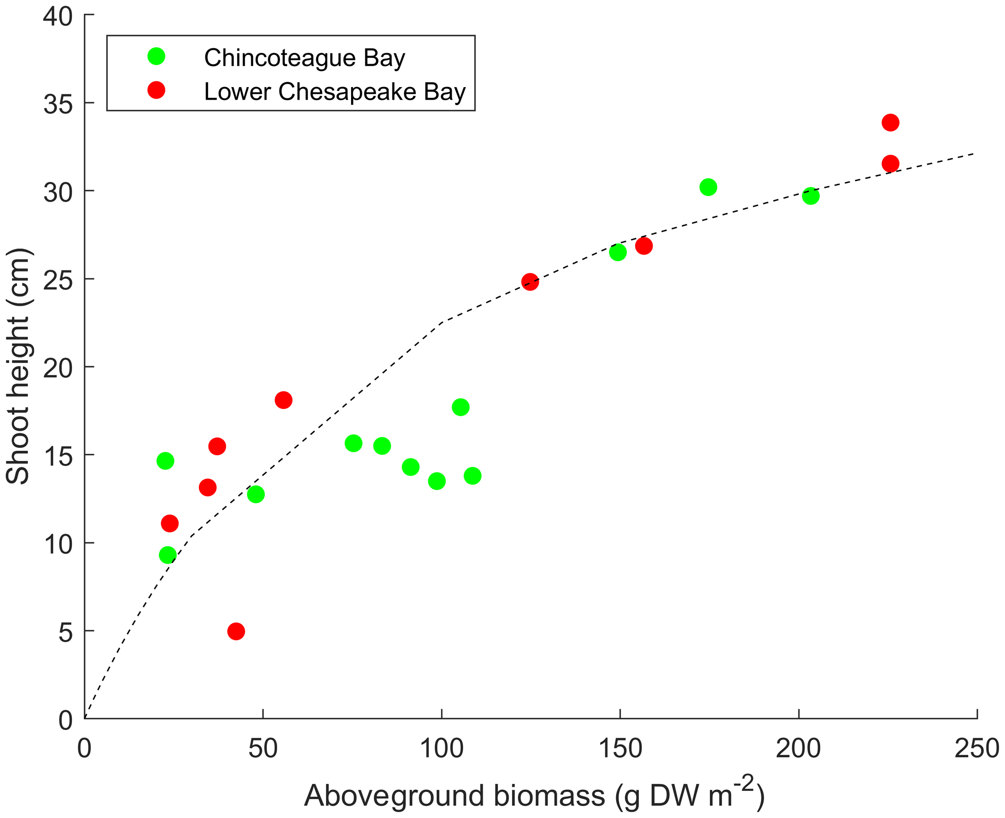
Figure 2Empirical relationships between aboveground biomass and SAV shoot height for Zostera marina populations in polyhaline regions of Chesapeake Bay and Chincoteague Bay. DW refers to dry weight. Data are from Moore (2004) and Ganju et al. (2018).

3.1 Idealized test case
The implementation of the SAV growth model within the COAWST framework is first tested on an idealized domain. The test case consists of an idealized rectangular domain of 9.2 km width and 9.8 km length with a 1 m deep basin. The number of interior domain points is 90 in the x direction and 98 in the y direction with 10 vertical sigma layers. The resulting domain has a grid resolution of 100 m by 100 m in horizontal and 0.1 m in vertical (this varies with water level) directions. A rectangular vegetation bed extends 8 km southward from the north boundary of the domain, with a width of 1.8 km, centered in the domain (Fig. 3). The ROMS barotropic and baroclinic time steps are 0.05 and 1 s, respectively. The bed roughness is set to zo=1.5 mm. The k−ε turbulence model is implemented following the GLS method (Warner et al., 2005). The initial AGB, BGB, and EPB in the vegetation bed are set to be 90, 15, and 0.01 mmol N m−2, respectively. The vegetation density, height, diameter, and thickness are initialized to be 400 stems m−2, 0.19 m, 1.0 mm, and 0.1 mm, respectively. The vegetative drag coefficient (CD) is set to be 1 (typical value for a cylinder at a high Reynolds number). The imposed surface wind speed is 3 m s−1 from the north to induce a wave field. The surface air pressure is initialized as 101.3 kPa. The kinematic surface solar shortwave radiation is set to an amplitude of 500.0 W m−2 with a 24 h period. The kinematic surface longwave radiation flux is set to zero (W m−2). The surface air temperature varies between 1.5 and 18.5 ∘C over a yearly period. The surface solar downwelling spectral irradiance just beneath the sea surface is set following Gregg and Carder (1990). The cloud fraction is set to be zero. The bulk flux parameterizations in COAWST for surface wind stress and surface heat flux are based on the Coupled Ocean-Atmosphere Response Experiment (COARE) code (Fairall et al., 1996a, b; Liu et al., 1979).
The model is forced by oscillating the water level on the northern boundary with a tidal amplitude of 0.25 m and a period of 12 h. Northern boundary conditions include a water temperature variation between 1.5 and 18.5 ∘C over a yearly period. Salinity and NO3 at the northern boundary are set to 35 psu and 20 mmol N m−3, respectively, and we impose a suspended sediment concentration of 0.5 g L−1 as well. The northern boundary condition for tracers is a radiation condition with nudging on a 6 h timescale. For both flow and tracer fields (physical and biological), the western and eastern boundaries have a gradient condition and the southern boundary is closed. The model setup for the idealized domain is simulated for 60 d and the model output is averaged over each day.
3.2 Realistic test case: West Falmouth Harbor, Massachusetts, USA
In their study, del Barrio et al. (2014) used an offline coupling of the COAWST model with a bio-optical seagrass model (Zimmerman et al., 2003) to study the influence of nitrate loading and sea-level rise on seagrass presence/absence in West Falmouth Harbor, Massachusetts, USA. Nitrate concentrations in groundwater exceeded 200 µM due to a wastewater treatment plant in the watershed; however, recent mitigation is expected to eliminate the nitrate load in the future. The model of del Barrio et al. (2014) used the biogeochemical results to generate spectral irradiance fields which were then passed to the bio-optical model. While useful for investigating the interaction between phytoplankton dynamics, light climate, and potential seagrass coverage, that model did not account for the interaction of seagrass with water column and sediment nitrogen pools or hydrodynamics. Therefore, we tested the fully coupled hydrodynamic, biogeochemical, and vegetation model using the same hydrodynamic and biogeochemical model setup (Ganju et al., 2012; del Barrio et al., 2014) but with the full vegetative interaction implemented. Briefly, the model is forced with tides at the western boundary, groundwater and nitrate loading at the eastern boundary, and solar irradiance at the air–sea boundary. Further details on the model setup are given by Ganju et al. (2012) and del Barrio et al. (2014). The hydrodynamic and biogeochemical (e.g., chlorophyll concentrations, light attenuation) results were assessed in those studies. In this work, we test the ability of the coupled model to reproduce the present-day spatial pattern of seagrass presence, with growth and persistence expected in the outer harbor and dieback in the inner harbor, where nitrate loading, phytoplankton growth, and light attenuation are highest. The initial SAV properties include a plant height of 0.195 m, plant density of 110 stems m−2, plant diameter of 0.001 m, and plant thickness of 0.0001 m. The vegetative drag coefficients CD in the flow model and the wave model are set to 1 (typical value for a cylinder at a high Reynolds number). We utilize the SAV growth model parameters described in Table 1. The model setup for West Falmouth Harbor (Sect. 3.2) is simulated for 56 d beginning 2 July 2010 (Ganju et al., 2012).

Figure 4Planform view of (a) depth-integrated suspended sediment concentration (SSC) and (b) light attenuation averaged over the last day of the simulation in the idealized domain.
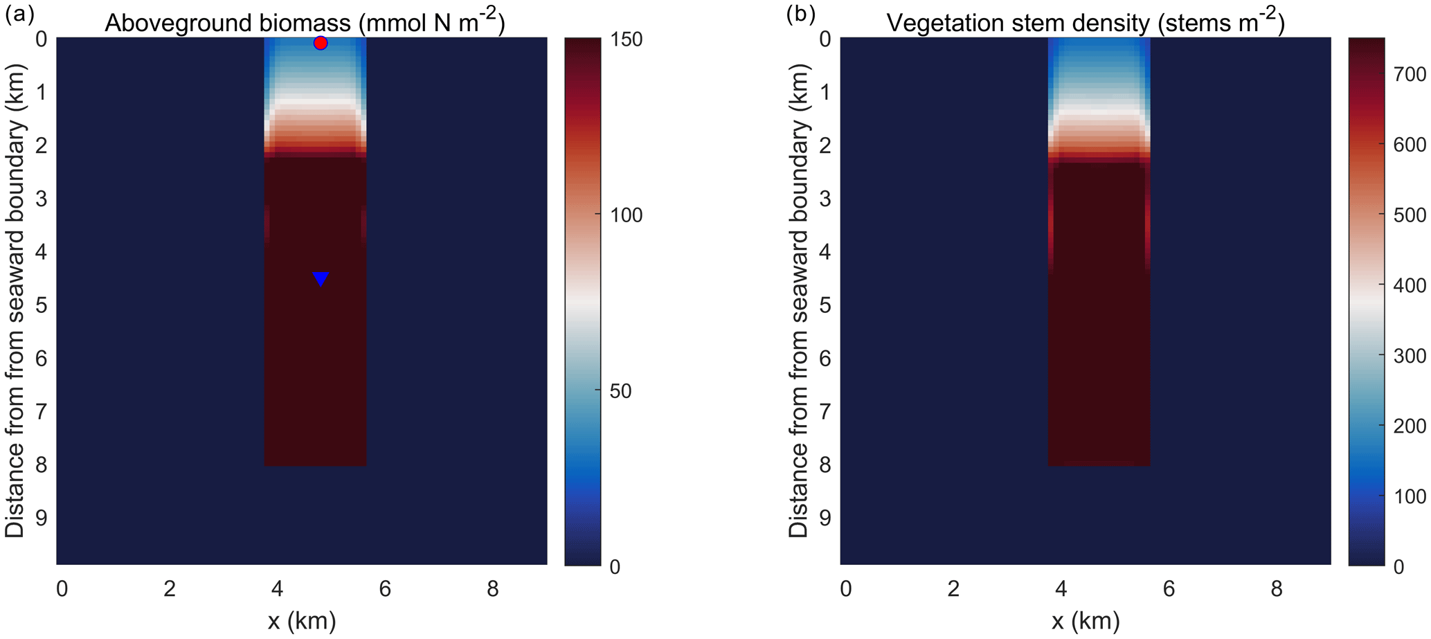
Figure 5Planform view of (a) aboveground biomass and (b) vegetation stem density averaged over the last day of the simulation in the idealized domain. The red dot and blue triangle represent two points that are located at 0.1 and 4.5 km into the SAV bed, respectively.
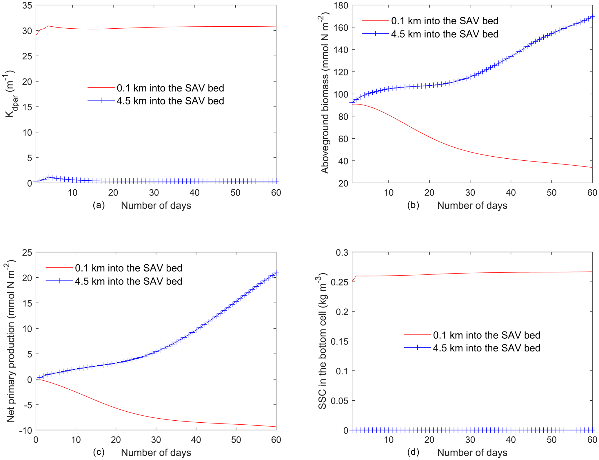
Figure 6Time series of (a) light attenuation, (b) aboveground biomass, (c) net primary production of SAV (), and (d) SSC in the bottom cell averaged every day from the two locations identified in Fig. 5a.
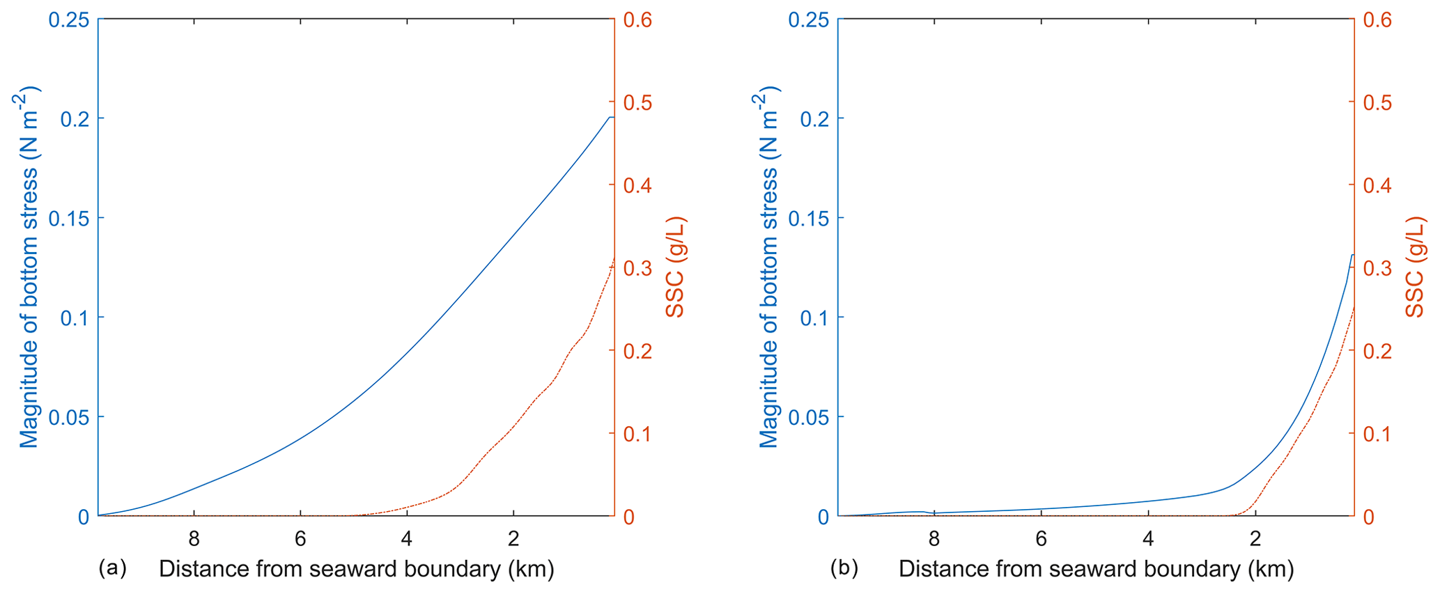
Figure 7Magnitude of bottom stress (a) and depth-integrated SSC (b) at the end of the simulation plotted along the y axis of the idealized domain at two locations, including one outside (x=1.8 km; panel a) and one inside the SAV bed (x=4.8 km, panel b).
4.1 SAV, sediment, and hydrodynamics in the idealized test case
Simulations of the coupled hydrodynamic–biogeochemical–SAV model revealed the integrated nature of estuarine dynamics in response to submerged macrophytes. In these simulations, suspended sediment concentration (SSC) was imposed at the northern open boundary at concentrations of 0.5 g L−1 (and 0 g L−1 within the bed), resulting in a decline in SSC as one moves towards the southern boundary (Fig. 4a). This distribution of SSC input results in an increase in light attenuation (Kdpar=30.0 m−1) in the region close to the northern boundary (0.0 km), while background conditions prevail in the southern reaches (Fig. 4b). In Fig. 4b, SSC input from the northern boundary causes a decrease in light availability within the modeled SAV region between the open boundary in the north and about 2.4 km into the SAV bed. Consequently, these suboptimal light conditions in the northern 2.4 km of the SAV bed cause AGB to decrease from its initial value of 90.0 to 30.0 mmol N m−2 (Fig. 5a). Boundary effects associated with SSC inputs are substantially muted in the region between 2.4 and 8.0 km within the SAV bed (Figs. 4 and 5), where in-bed SSCs are much lower than those outside the bed at the same distance from the boundary. As a consequence, AGB biomass increases from its initial value of 90.0 to 150.0 mmol N m−2 over the course of the simulation. Increases in SAV biomass within the bed during the simulation led to increases in SAV density and height, where SAV density increased from its initial value of 400 to 810 stems m−2 due to favorable light conditions from y=2.4 km to y=8.0 km. Thus, the model captured the role of SAV in resisting SSC transport into the bed, allowing for greater light availability and an increase in growth rates and biomass accumulation.
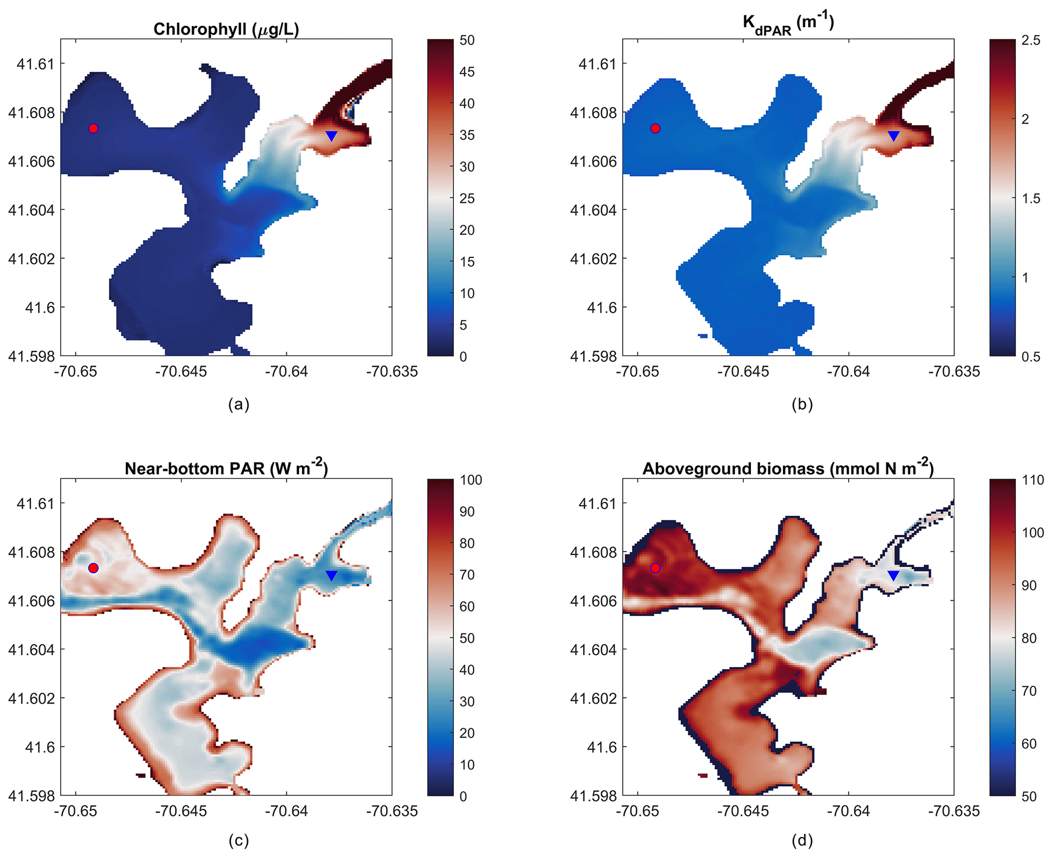
Figure 8Mean over 22 d of (a) depth-averaged chlorophyll, (b) light attenuation, (c) near-bottom PAR, and (d) peak aboveground biomass on day 14 of the simulation. The red circle indicates the outer harbor (a, c) and the blue triangle indicates the inner harbor (b, d) points for time-series data in Fig. 9.
The temporal evolution of SAV biomass in response to the SSC input at the northern boundary further emphasizes the self-stimulating role of SAV in the idealized simulations. A comparison of model simulations at two locations within the initially described SAV bed of the idealized domain (indicated in Fig. 5a and corresponding to y=0.1 km and y=4.5 km from the northern boundary) reveals that close to the northern boundary (y=0.1 km), the daily averaged light attenuation remains high (above 30 m−1) over the 60 d period (Fig. 5a). At y=0.1 km, the increased light attenuation in the northern location corresponds to the lack of light availability and this causes a decay of AGB from its initial value of 90.0 to 30.0 mmol N m−2. (Fig. 5b). This decay in AGB over the 60 d period at y=0.1 km (SAV dieback) contrasts sharply with the AGB increases inside the SAV bed at the southern location (y=4.5 km), where light attenuation is lower because sediments have not penetrated the SAV bed, allowing for higher SAV growth rates. The higher SAV growth rate inside the SAV bed at y=4.5 km can be observed (Fig. 5c) by looking at the net primary production of SAV (). At this location (y=4.5 km), the SAV growth rate increases over the 60 d period while it keeps decreasing in the northern location (y=0.1 km). Due to the higher SAV growth inside the SAV bed (y=4.5 km), the SSC in the bottom cell remains low (Fig. 5d) and at y=0.1 km due to the SAV dieback; the sediment concentration in the water column stays high and above 0.25 g L−1.
As mentioned above, the SSC input on the northern boundary of the idealized domain causes a region of suboptimal light conditions that lead to the SAV dieback, while the SAV growth occurs in the remaining bed where favorable light conditions exist. The effect of change in SAV density and height on the hydrodynamics and morphodynamics at the end of the simulation can be demonstrated by using the same idealized domain. To this end, two transects are chosen that are along the length of the SAV bed and extend from the northern boundary towards the southern boundary. The transects are chosen inside at x=1.8 km (outside of the SAV bed) and at x=4.8 km (inside of the SAV bed). The depth-integrated SSC and bottom stresses averaged on the 60th day in the transect (Fig. 7a) outside of the SAV bed show that the profile of bottom stress follows the distribution of SSC along the transect. In Fig. 7a, a peak bottom stress of about 0.2 N m−2 is obtained at x=1.8 km (outside of the SAV bed) that corresponds to a depth-averaged SSC of 0.31 g L−1. On the other hand, the transect within the SAV bed (Fig. 7b) shows that the region where SAV dieback has occurred (between 0.0 and 2.4 km) corresponds to increased bottom stresses (0.13 N m−2 at the northernmost location and a corresponding SSC of 0.26 g L−1), while in the region where the SAV growth has occurred, the bottom stresses are close to zero (i.e., from 2.4 km onwards).
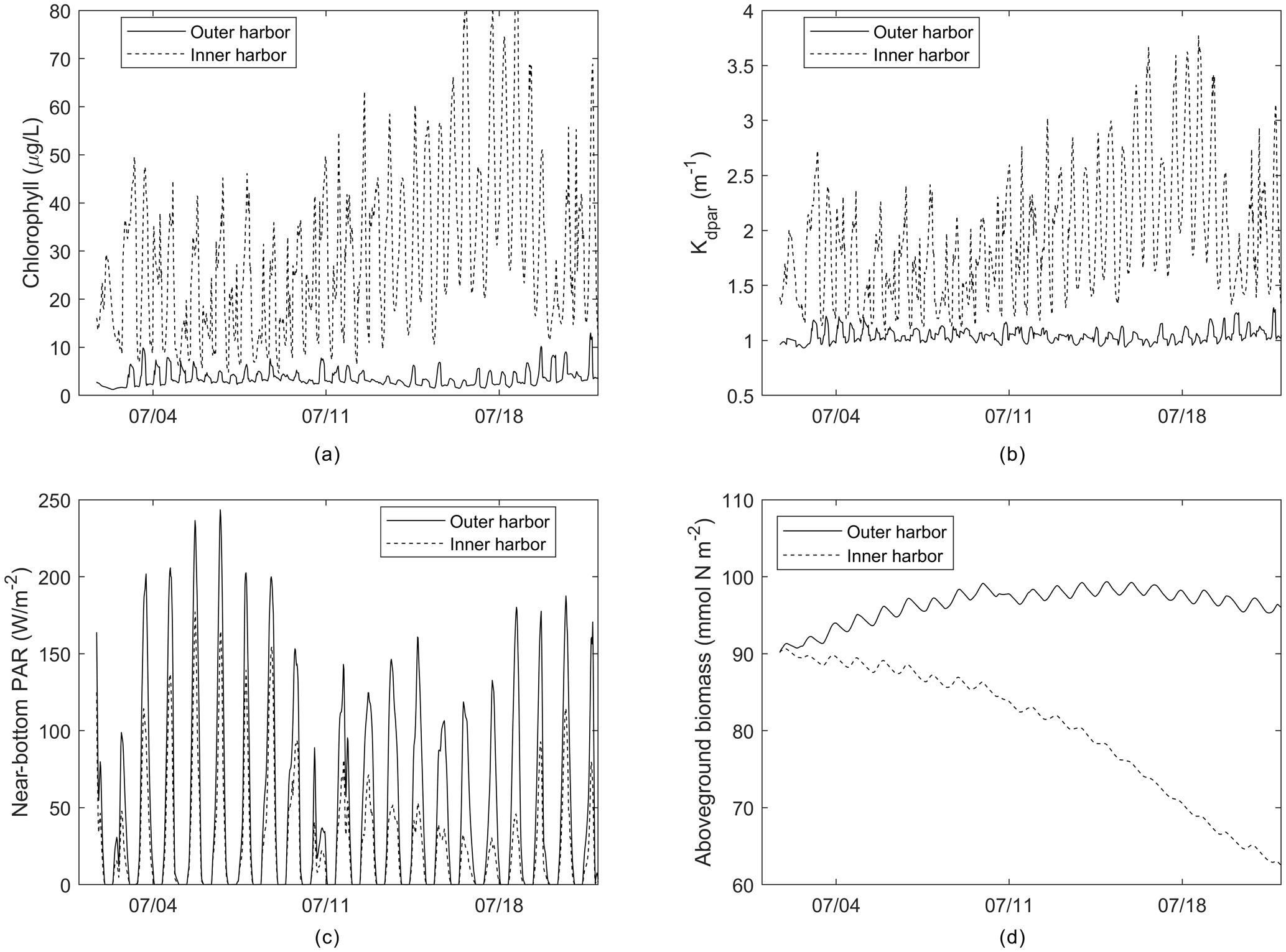
Figure 9Time series of (a) chlorophyll, (b) light attenuation, (c) near-bottom PAR, and (d) aboveground biomass from outer and inner harbor locations identified in Fig. 6.
The simulation of the idealized domain demonstrates the capability of the modeling framework to perform two-way feedbacks between hydrodynamics, sediment, and biological dynamics. The SSC input in the northern boundary affects the light attenuation in the domain and causes SAV dieback close to the northern boundary. The SAV grows in the region where favorable light conditions exist. The SAV dieback leads to increased bottom stresses, while the growth of SAV leads to a decrease in bottom stresses, illustrating the fact that the SAV acts as bottom sediment stabilizer by reducing SSC.
4.2 SAV growth in West Falmouth Harbor
The present-day simulation of seagrass dynamics reproduces the patterns of chlorophyll (via phytoplankton), light attenuation, and near-bottom PAR simulated by del Barrio et al. (2014). Nitrate loading from shoreline point sources led to increased phytoplankton growth indicated by increased chlorophyll and light attenuation in the landward, northeast portion of the harbor (Fig. 8a, b), while bathymetric controls in the deeper central basin led to decreased near-bottom PAR (Fig. 8c). Peak AGB exceeds 100 mmol N m−2, while seagrass presence begins towards decline in the inner harbor and in the central basin as expected. Intertidal areas around the periphery of the harbor are devoid of AGB due to the enforced masking of areas with intermittent wetting and drying.
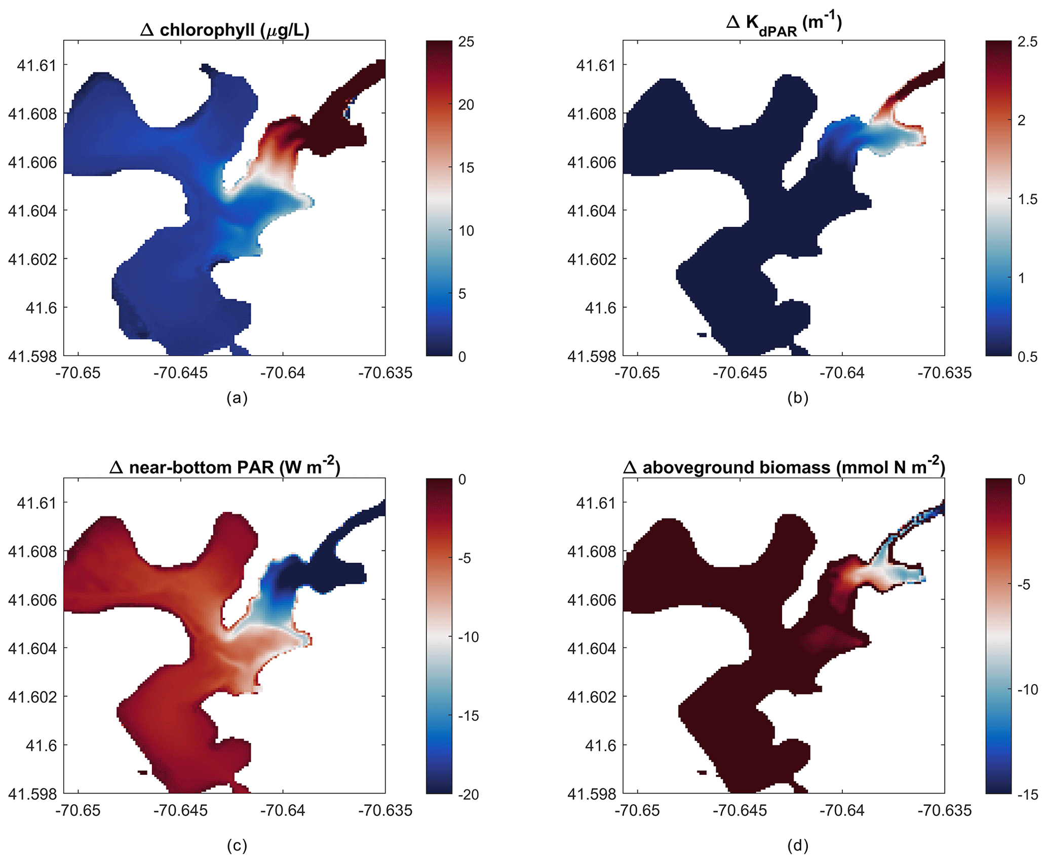
Figure 10Change in outcomes between impacted and non-impacted scenarios (nitrate loading scenario – no loading scenario). Difference in mean over 22 d of (a) depth-averaged chlorophyll, (b) light attenuation, (c) near-bottom PAR, and (d) peak aboveground biomass on day 14 of the simulation.
Time series of these parameters (Fig. 9) from selected outer and inner harbor locations over the first 22 d demonstrate the diurnal variability, as well as the rapid loss of AGB in the inner harbor due to the local nitrate loading, phytoplankton proliferation, and degraded light climate. The sizable diurnal variability in AGB (Fig. 9d) appears to be an artifact of production/respiration formulations that are based on seasonal responses to environmental forcing, rather than diurnal responses to solar irradiance. Future modifications could attenuate this variability by utilizing daily averaged environmental forcing or modifying the frequency of biomass updating.
The modeling framework developed in this work can be used to create hypothetical scenarios to estimate future environmental responses. For example, we ran the model setup of West Falmouth Harbor described in Sect. 3.2 with no nitrate loading to simulate a hypothetical scenario where the groundwater input has no influence from the wastewater treatment plant (non-impacted past or future scenario). The elimination of nitrate loading results in negligible changes in the outer harbor but greatly reduces chlorophyll and light attenuation in the inner harbor (Fig. 10a, b), while increasing the near-bottom PAR (Fig. 10c). Peak AGB responds to the decreased chlorophyll and increased light attenuation with an increase in the inner harbor (Fig. 10d). This implementation represents an incremental improvement to the prior modeling exercise (Ganju et al., 2012; del Barrio et al., 2014), because the interactions between SAV and the nitrogen pools are explicitly accounted for. For example, this model can now be used to test how changes in seagrass coverage influence nitrogen retention within the estuary or export to the coastal ocean. Further, the introduction of seagrass kinetics will allow for investigation of water-column oxygen budgets with and without seagrass under present and future scenarios.
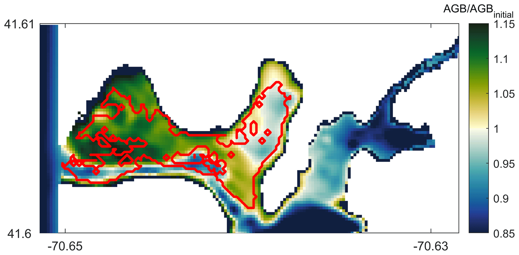
Figure 11Modeled AGB∕AGBinitial (aboveground biomass) distribution compared with field data showing seagrass coverage extent (solid red line). Values of represent seagrass growth potential and those below 1 indicate potential seagrass decline on day 14 of the simulation.
4.3 Model evaluation in West Falmouth Harbor
In order to qualitatively evaluate the seagrass growth model, we have compared the modeled results with observations by del Barrio et al. (2014) that measured the extent of seagrass coverage in West Falmouth Harbor (red outline in Fig. 11). The field data are only available for the northern region of West Falmouth Harbor where the model–data comparisons are performed. The model results are compared by extracting the peak AGB on 14th day of the simulation and normalized with the initial aboveground biomass. The ratio of AGB∕AGBinitial is considered as a representative of seagrass growth. We assume that for , there is a potential for seagrass growth, and for , the conditions are unfavorable for seagrass growth. In Fig. 11, the model and field data show an 89 % agreement to determine the seagrass growth or dieback. The western region of outer harbor shows seagrass growth potential and agrees with the extent that the seagrass coverage is observed. In the eastern region, the field data show no seagrass coverage and the model also predicts potential seagrass dieback. The model predicts seagrass dieback because of nitrate loading from shoreline point sources that leads to increased chlorophyll and light attenuation (Fig. 8a, b). The model and observations do not compare well in the central basin of outer harbor where the model shows seagrass dieback potential, while the field data show the presence of seagrass. In the central basin, the field data show the presence of seagrass while its density remains low in this region. On the other hand, the modeled seagrass suffers dieback due to the bathymetric controls in the deeper central basin (decreased near-bottom PAR; Fig. 8c).
Direct estimates of aboveground SAV biomass have also been recently made in West Falmouth Harbor (Hayn et al., unpublished data). Although these measurements were not made during the same year as our simulations (measurements in 2006, 2007, 2013; model 2010), the mean aboveground biomass measured in the outer harbor of 49.5 (21 June–6 July 2006), 45.3 (6–19 June 2007), and 41.5 g C m−2 (15–19 July 2013) is consistent with the range of model simulations during a comparable period (2–19 July) in the outer (28.1 to 51.1 g C m−2) and middle (14.9 to 37.4 g C m−2) harbors. The 2–19 July model range of 45.7 to 156.3 mmol N m−2 across the middle and outer harbors is also consistent with annual mean Z. marina biomass (10–88 mmol N m−2) reported in nearby shallow systems on Cape Cod (Hauxwell et al., 2003) assuming a literature-based average that aboveground SAV biomass is 1.5 % N. The range in the model is computed based on the minimum and maximum values of AGB during the 18 d simulation period.
4.4 Limitations of SAV growth model and future work
While this modeling approach represents an advance in modeling coupled biophysical processes in estuaries, there are limitations that must be addressed in future work:
-
The modeling of SAV dieback/growth scenarios may require long-term simulations on decadal timescales (Carr et al., 2018). However, the short model time step limits the duration of such simulations. The time step size is of the order of seconds (typical of 3-D ocean models) and this, combined with the fact that the presence of SAV in the hydrodynamic model further limits time step size (due to hydrodynamic stability constraints), overall limits the applicability of the model to be utilized from monthly to annual timescales at this juncture.
-
The biomass equations described in Sect. 2.3 are formulated for seasonal timescales and are being used in the model implementation at every ocean model time step. This leads to large daily variations in above- and belowground biomass that likely do not occur in the environment, although diel variations on SAV growth have been measured in situ (Kemp et al., 1987). Hence, with the current formulations, the output from the biomass model needs to be analyzed as a daily averaged quantity.
-
The current implementation of the SAV growth model is limited to only one SAV species. However, it should be extended to include multiple SAV species to investigate competition under variable salinity and to make the model applicable to a wider variety of locations.
The present study adds to the open-source COAWST modeling framework by implementing a SAV growth model. Based on the change in SAV (aboveground, belowground) biomass and epiphyte biomass, SAV density and height evolve in time and space and directly couple to three-dimensional water-column biogeochemical, hydrodynamic, and sediment transport models. SAV biomass is computed from temperature, nutrient loading, and light predictions obtained from coupled hydrodynamics (temperature), biogeochemistry (nutrients), and bio-optical (light) models. In exchange, the growth of SAV sequesters or contributes nutrients from the water column and sediment layers. The presence of SAV modulates current and wave attenuation and consequently affects modeled sediment transport and fate. The resulting modeling framework provides a two-way coupled SAV–biogeochemistry–hydrodynamic and morphodynamic model. This allows for the simulation of the dynamic growth and mortality of SAV in coastal environments in response to changes in light and nutrient availability, including SAV impacts on sediment transport and nutrient, carbon, and oxygen cycling. The implementation of the model is successfully tested in an idealized domain where the introduction of sediment in the water column (SSC) at one end of the domain provides suboptimal light conditions that cause SAV dieback in that region. The model was applied to the temperate estuary of West Falmouth Harbor, where simulations show the coupled effect of enhanced nitrate loading in the inner harbor leading to poor light conditions for the SAV to grow, thus modeling the physical effect of eutrophication leading to the loss of a SAV habitat. Among other applications, in the future, the model will be used assess the effects of sea-level-rise scenarios that limit light availability and potentially cause the loss of SAV habitats.
The implementation of the SAV growth model has been conducted within COAWST v3.4. This particular version is available for download at https://www.sciencebase.gov/catalog/item/5f15d69082cef313ed81996a (last access: 23 April 2019) (Warner et al., 2019, https://doi.org/10.5066/P9NQUAOW). Users are encouraged to download COAWST, which is distributed through the US Geological Survey (USGS) code archival repository. It is available for download at https://code.usgs.gov/coawstmodel/COAWST (last access: 18 May 2020). The COAWST distribution files contain source code derived from ROMS, SWAN, WRF, MCT, and SCRIP, along with the MATLAB code, examples, and a user manual.
The major code development that was done for this project is contained within the COAWST folder on the following path: https://code.usgs.gov/coawstmodel/COAWST/blob/master/ROMS/Nonlinear/Biology/ (last access: 13 March 2019).
This folder contains several methods of computing water-column biogeochemistry. Other than the I/O component of our implementation, the algorithmic development in this study only modifies two files on this path: “estuarybgc.h” and “sav_biomass.h”. The file “sav_biomass.h” contains all the newly added equations for the growth of SAV based on the nutrient loading in the water column. The forcings to the SAV growth model (temperature, light, nutrient availability, exchanges nutrients, detritus, dissolved inorganic carbon, and dissolved oxygen) are provided through the file “estuarybgc.h” which calls “sav_biomass.h”. The file “estuarybgc.h” solves for the water-column biogeochemistry and was based on existing modeling framework developed by Fennel et al. (2006) (also coded as “fennel.h”).
Other important paths that existed in the framework prior to the current modeling effort but are being used in the modeling process include the following:
-
The main kernel of the 3-D non-linear Navier–Stokes equations is contained within this part and links all the submodels: biological, vegetation, and sediment models; https://code.usgs.gov/coawstmodel/COAWST/blob/master/ROMS/Nonlinear (last access: 13 March 2019).
-
The kernels that account for seagrass–hydrodynamics interactions can be found here: https://code.usgs.gov/coawstmodel/COAWST/blob/master/ROMS/Nonlinear/Vegetation/ (last access: 13 March 2019).
-
The kernels that account for sediment transport can be found here: https://code.usgs.gov/coawstmodel/COAWST/blob/master/ROMS/Nonlinear/Sediment/ (last access: 13 March 2019).
The model data were released as per the USGS model data release policy, and separate digital object identifiers were created as part of the release (https://www.usgs.gov/products/data-and-tools/data-management/data-release, last access: 10 June 2019). The model output can be accessed through ScienceBase entries for the idealized test case simulation (Kalra and Ganju, 2019, https://doi.org/10.5066/P973NL8J) and West Falmouth Harbor simulations (Ganju and Kalra, 2019, https://doi.org/10.5066/P998IJGG).
TSK implemented the SAV growth model in the COAWST framework. JMT provided guidance on the mechanistic processes affecting the growth of SAV from biomass parameterizations and developed linkages between the SAV growth model and the water-column biogeochemical model. NKG developed the test case and the realistic domain case. TSK and NKG performed the data analysis from the output of the test cases and were responsible for model data release. The paper was prepared with contributions from all co-authors.
The authors declare that they have no conflict of interest.
Any use of trade, firm, or product names is for descriptive purposes only and does not imply endorsement by the US Government.
We thank Joel Carr at the US Geological Survey Patuxent Wildlife Research Center in Beltsville, Maryland, for providing his feedback to improve the quality of the paper. We thank the reviewers for their careful reading of our manuscript and their insightful comments and suggestions. We thank Alfredo Aretxabaleta for valuable discussions through the length of the project. We would also like to thank Melanie Hayn, Robert Howarth, Roxanne Marino, and Karen McGlathery for sharing Z. marina biomass measurements from West Falmouth Harbor collected with funding from the National Science Foundation and Woods Hole SeaGrant to Cornell University. All the contour plots were generated using the “cmocean” package developed by Thyng et al. (2016). The authors thank VeeAnn Cross and associated staff at USGS that helped in model data release in a timely manner. This is University of Maryland Center for Environmental Contribution no. 5909.
This paper was edited by David Ham and reviewed by Jon Hill and David Ham.
Arakawa, A. and Lamb, V. R.: Computational design of the basic dynamical processes of the UCLA general circulation model, Methods in Computational Physics: Advances in Research and Applications, 17, 173–265, 1977.
Beudin, A., Kalra, T. S., Ganju, N., K., and Warner, J. C.: Development of a Coupled Wave-Current-Vegetation Interaction, Comput. Geosci., 100, 76–86, 2017.
Bissett, W. P., Carder, K. L., Walsh, J. J., and Dieterle, D. A.: Carbon cycling in the upper waters of the Sargasso Sea: I. Numerical simulation of differential carbon and nitrogen fluxes, Deep-Sea Res. Pt. I, 46, 205–269, 1999a.
Bissett, W. P., Carder, K. L., Walsh, J. J., and Dieterle, D. A.: Carbon cycling in the upper waters of the Sargasso Sea: II. Numerical simulation of apparent and inherent optical properties, Deep-Sea Res. Pt. II, 46, 271–317, 1999b.
Booij, N., Ris, R. C., and Holthuijsen, L. H.: A third-generation wave model for coastal regions, Part I, Model description and validation, J. Geophys. Res., 104, 7649–7666, 1999.
Burkholder, J. M., Tomasko, D. A., and Touchette, B. W.: Seagrasses and eutrophication, J. Exp. Mar. Biol. Ecol., 350, 46–72, 2007.
Cabello-Pasini, A., Muniz-Salazar, R., and Ward, D. H.: Annual variations of biomass and photosynthesis in Zostera marina at its southern end of distribution in the North Pacific, Aquat. Bot., 76, 31–47, 2003.
Carr, J., D'Odorico, P., McGlathery, K., and Wiberg, P.: Stability and bistability of seagrass ecosystems in shallow coastal lagoons: role of feedbacks with sediment resuspension and light attenuation, J. Geophys. Res., 115, G03011, https://doi.org/10.1029/2009JG001103, 2010.
Carr, J. A., D'Odorico, P., McGlathery, K. J., and Wiberg, P. L.: Stability and resilience of seagrass meadows to seasonal and interannual dynamics and environmental stress, J. Geophys. Res., 117, G01007, https://doi.org/10.1029/2011JG001744, 2012a.
Carr, J. A., D'Odorico, P., McGlathery, K. J., and Wiberg, P. L.: Modeling the effects of climate change on eelgrass stability and resilience: future scenarios and leading indicators of collapse, Mar. Ecol. Prog. Ser., 448, 289–301, 2012b.
Carr, J., Mariotti, G., Fahgerazzi, S., McGlathery, K., and Wiberg, P.: Exploring the Impacts of Seagrass on Coupled Marsh-Tidal Flat Morphodynamics, Front. Environ. Sci., 6, 1–16, 2018.
Cerco, C. F. and Moore, K.: System-wide submerged aquatic vegetation model for Chesapeake Bay, Estuaries, 24, 522–534, 2001.
Chassignet, E. P., Arango, H. G., Dietrich, D., Ezer, T., Ghil, M., Haidvogel, D. B., Ma, C.-C., Mehra, A., Paiva, A. M., and Sirkes, Z.: DAMEE-NAB: The base experiments, Dyn. Atmos. Ocean., 32, 155–183, 200.
Colella, P. and Woodward, P. R.: The Piecewise Parabolic Method (PPM) for gas-dynamical simulations, J. Comput. Phys., 54, 174–201, 1984.
del Barrio, P., Ganju, N. K., Aretxabaleta, A. L., Hayn, M., García, A., and Howarth, R. W.: Modeling future scenarios of light attenuation and potential seagrass success in a eutrophic estuary, Estuarine, Coast. Shelf Sci., 149, 13–23, 2014.
Everett, J. D., Baird, M. E., and Suthers, I. M.: Nutrient and plankton dynamics in an intermittently closed/open lagoon, Smiths Lake, south-eastern Australia: an ecological model, Estuarine, Coast. Shelf Sci., 72, 690–702, 2007.
Fairall, C. W., Bradley, E. F., Godfrey, J. S., Wick, G. A., Edson, J. B., and Young, G. S.: Cool-skin and warm-layer effects on sea surface temperature, J. Geophys. Res., 101, 1295–1308, 1996a.
Fairall, C. W., Bradley, E. F., Rogers, D. P., Edson J. B., and Young, G. S.: Bulk parameterization of air-sea fluxes for tropical ocean global atmosphere Coupled-Ocean Atmosphere Response Experiment, J. Geophys. Res., 101, 3747–3764, 1996b.
Fennel, K., Wilkin, J., Levin, J., Moisan, J., O'Reilly, J., and Haidvogel, D.: Nitrogen cycling in the Middle Atlantic Bight: results from a three-dimensional model and implications for the North Atlantic nitrogen budget, Global Biogeochem. Cy., 20, GB3007, https://doi.org/10.1029/2005GB002456, 2006.
Gallegos, C. L., Werdell, P. J., McClain, C. R.: Long-term changes in light scattering in Chesapeake Bay inferred from Secchi depth, light attenuation, and remote sensing measurements, J. Geophys. Res., 116, C00H08, https://doi.org/10.1029/2011JC007160, 2011.
Ganju, N. K. and Kalra, T. S.: Numerical model of Submerged Aquatic Vegetation (SAV) growth dynamics in West Falmouth Harbor, U.S. Geological Survey data release, https://doi.org/10.5066/P998IJGG, 2019.
Ganju, N. K., Hayn, M., Chen, S. N., Howarth, R. W., Dickhudt, P. J., Aretxabaleta, A. L., and Marino, R.: Tidal and groundwater fluxes to a shallow, microtidal estuary: constraining inputs through field observations and hydrodynamic modeling, Estuar. Coasts, 35, 1285–1298, 2012.
Ganju, N. K., Testa, J. M., Suttles, S. E., and Aretxabaleta, A. L.: Spatiotemporal variability of light attenuation and net ecosystem metabolism in a back-barrier estuary, Biogeosciences Discuss., https://doi.org/10.5194/bg-2018-335, 2018.
Ghisalberti, M. and Nepf, H. M.: The limited growth of vegetated shear layers, Water Resour. Res., 40, W07502, https://doi.org/10.1029/2003WR002776, 2004.
Ghisalberti, M. and Nepf, H. M.: The structure of the shear layer in flows over rigid and flexible canopies, Environ. Fluid Mech., 6, 277–301, 2006.
Gregg, W. W. and Carder, K. L.: A simple spectral solar irradiance model for cloudless maritime atmospheres, Limnol. Oceanogr., 35, 1657–1675, 1990.
Haidvogel, D. B., Arango, H. G., Hedstrom, K., Beckmann, A., Malanotte-Rizzoli, P., and Shchepetkin, A. F.: Model evaluation experiments in the North Atlantic Basin: simulations in nonlinear terrain-following coordinates. Dynamics of Atmosphere Oceans, 32, 239–281, 2000.
Haidvogel, D. B., Arango, H. G., Budgell, W. P., Cornuelle, B. D., Curchitser, E., Di Lorenzo E., Fennel, K., Geyer, W. R., Hermann, A. J., Lanerolle, L., Levin, McWilliams, J. C., Miller, Moore, A. M., Powell, T. M., Shchepetkin, A. F., Sherwood, C. R., Signell, R. P., Warner, J. C., and Wilkin, J.: Ocean forecasting in terrain-following coordinates: Formulation and skill assessment of the Regional Ocean Modeling System, J. Comput. Phys., 227, 3595–3624, 2008.
Hamberg, J., Findlay, S. E. G., Limburg, K. E., and Diemont, S. A. W.: Post‐storm sediment burial and herbivory of Vallisneria americana in the Hudson River estuary: mechanisms of loss and implications for restoration, Restor. Ecol., 25, 629–639, https://doi.org/10.1111/rec.12477, 2017.
Hauxwell, J., Cebrian, J., and Valiela, I.: Eelgrass Zostera marina loss in temperate estuaries: relationship to land-derived nitrogen loads and effect of light limitation imposed by algae, Mar. Ecol. Prog. Ser., 247, 59–73, https://doi.org/10.3354/meps247059, 2003.
Hayn, M., Howarth, R. W., Marino, M., Ganju, N., Berg, P., Foreman, K., Giblin, A., and McGlathery, K.: Exchange of nitrogen and phosphorus between a shallow lagoon and coastal waters, Estuar. Coasts, 37, S63–S73, 2014.
Hemming, M. A. and Duarte, C. M.: Seagrass Ecology, Cambridge University Press, Limnol. Oceanogr., 2, https://doi.org/10.4319/lo.2002.47.2.0611, 2000.
Hipsey, M. R. and Hamilton, D. P.: Computational Aquatic Ecosystem Dynamic Model: CAEDYM v3 Science Manual, Centre for Water Research, University of Western Australia, 2008.
Jarvis, J. C., Brush, M. J., and Moore, K. A.: Modeling loss and recovery of Zostera marina beds in the Chesapeake Bay: the role of seedlings and seed-bank viability, Aquat. Bot., 113, 32–45, 2014.
Kalra, T. S. and Ganju, N. K.: Idealized numerical model for Submerged Aquatic Vegetation (SAV) growth dynamics, U.S. Geological Survey data release, https://doi.org/10.5066/P973NL8J, 2019.
Kalra, T. S., Li, X., Warner, J. C., Geyer, W. R., and Wu, H.: Comparison of Physical to Numerical Mixing with Different Tracer Advection Schemes in Estuarine Environments, J. Marine Sci. Eng., 7, e338–e361, 2019.
Kemp, W., Murray, L., Borum, J., and Sand-Jensen, K.: Diel growth in eelgrass Zostera marina, Marine Ecol. Prog. Ser., 41, 79–86, 1987.
Kennish, M. J., Sakowicz, G. P., and Fertig, B.: Recent Trends of Zostera marina (Eelgrass) in a Highly Eutrophic Coastal Lagoon in the Mid-Atlantic Region (USA), Open J. Ecol., 6, 243–253, 2016.
Krause-Jensen, D., Middelboe, A. L., Sand-Jensen, K., and Christensen, P. B.: Eelgrass, Zostera marina, growth along depth gradients: upper boundaries of the variation as a powerful predictive tool, Oikos, 91, 233–244, 2000.
Larkum, A. W., Orth, R. J., and Duarte, C. M.: Seagrasses: Biology, Ecology and Conservation, Springer, The Netherlands, 2006.
Liu, W. T., Katsaros, K. B., and Businger, J. A.: Bulk parameterization of the air-sea exchange of heat and water vapor including the molecular constraints at the interface, J. Atmos. Sci., 36, 1722–1735, 1979.
Madden, C. J. and Kemp, W. M..: Ecosystem Model of an Estuarine Submersed Plant Community: Calibration and Simulation of Eutrophication Responses, Estuarine Research Foundation, 19, 457–474, 1996.
McGlathery, K. J., Sundback, K., and Anderson, I. C.: Eutrophication in shallow coastal bays and lagoons: the role of plants in the coastal filter, Marine Ecol. Prog. Ser., 348, 1–18, 2007.
Moore, K. A.: Influence of Seagrasses on Water Quality in Shallow Regions of the Lower Chesapeake Bay, J. Coast. Res., 162–178, 2004.
Nixon, S. W., Buckley, B., Granger, S., and Bintz, J.: Responses of very shallow marine ecosystems to nutrient enrichment, Human Ecological Risk Assessment: An International Journal, 7, 1457–1481, 2001.
Shchepetkin, A. F. and McWilliams, J. C.: The Regional Ocean Modeling System: A split-explicit, free-surface, topography-following coordinates ocean model, J. Ocean Model., 9, 347–404, 2005.
Shchepetkin, A. F. and McWilliams, J. C.: Computational Kernel Algorithms for Fine-Scale, Multiprocess, Longtime Oceanic Simulations, Handbook of Numerical Analysis, 14, 121–183, 2009.
Short, F. T. and Neckles, H. A.: The Effects of Global Climate Change on Seagrasses, Aquat. Bot., 63, S0304–3770, 1999.
Smolarkiewicz, P. K.: A fully multidimensional positive definite advection transport algorithm with small implicit diffusion, J. Comput. Phys., 54, 325–362, 1984.
Terrados, J. and Borum, J.: Why are seagrasses important? Goods services provided by seagrass meadows, in: European seagrasses: an introduction to monitoring and management, 8–10, 2006.
Thyng, K. M., Greene, C. A., Hetland, R. D., Zimmerle, H. M., and DiMarco, S. F.: True colors of oceanography, Oceanography, 29, 9–13, 2016.
Warner, J. C., Sherwood, C. R., Signell, R. P., Harris, C. K., and Arango, H. G.: Development of a three-dimensional, regional, coupled wave, current, and sediment-transport model, Comput. Geosci., 34, 1284–1306, 2008.
Warner, J. C., Armstrong, B., He, R., and Zambon, J. B.: Development of a Coupled Ocean-Atmosphere-Wave-Sediment Transport (COAWST) Modeling System, Ocean Model., 35, 230–244, 2010.
Warner, J. C., Ganju, N. K., Sherwood, C. R., Tarandeep, K., Aretxabaleta, A., He, R., Zambon, J., and Kumar, N.: Coupled-Ocean-Atmosphere-Wave-Sediment Transport (COAWST) Modeling System: U.S. Geological Survey Software Release, 23 April 2019, https://doi.org/10.5066/P9NQUAOW, 2019.
Zaldívar, J. M., Bacelar, F. S., Dueri, S., Marinov, D., Viaroli, P., and Hernández-García, E.: Modeling approach to regime shifts of primary production in shallow coastal ecosystems, Ecol. Model., 220, 3100–3110, 2009.
Zharova, N., Sfriso, A., Voinov, A., and Pavoni, B.: A simulation model for the annual fluctuation of Zostera Marina biomass in the Venice lagoon, Aquat. Bot., 70, 135–150, 2001.
Zimmerman, R. C.: A biooptical model of irradiance distribution and photosynthesis in seagrass canopies, Limnol. Oceanogr., 48, 568–585, 2003.