the Creative Commons Attribution 4.0 License.
the Creative Commons Attribution 4.0 License.
 | 30 Oct 2020
Collisional growth in a particle-based cloud microphysical model: insights from column model simulations using LCM1D (v1.0)
Simon Unterstrasser
Fabian Hoffmann
Marion Lerch
Lagrangian cloud models (LCMs) are considered the future of cloud microphysical modelling. Compared to bulk models, however, LCMs are computationally expensive due to the typically high number of simulation particles (SIPs) necessary to represent microphysical processes such as collisional growth of hydrometeors successfully. In this study, the representation of collisional growth is explored in one-dimensional column simulations, allowing for the explicit consideration of sedimentation, complementing the authors' previous study on zero-dimensional collection in a single grid box. Two variants of the Lagrangian probabilistic all-or-nothing (AON) collection algorithm are tested that mainly differ in the assumed spatial distribution of the droplet ensemble: the first variant assumes the droplet ensemble to be well-mixed in a predefined three-dimensional grid box (WM3D), while the second variant considers the (sub-grid) vertical position of the SIPs, reducing the well-mixed assumption to a two-dimensional, horizontal plane (WM2D). Since the number of calculations in AON depends quadratically on the number of SIPs, an established approach is tested that reduces the number of calculations to a linear dependence (so-called linear sampling). All variants are compared to established Eulerian bin model solutions. Generally, all methods approach the same solutions and agree well if the methods are applied with sufficiently high resolution (foremost is the number of SIPs, and to a lesser extent time step and vertical grid spacing). Converging results were found for fairly large time steps, larger than those typically used in the numerical solution of diffusional growth. The dependence on the vertical grid spacing can be reduced if AON-WM2D is applied. The study also shows that AON-WM3D simulations with linear sampling, a common speed-up measure, converge only slightly slower compared to simulations with a quadratic SIP sampling. Hence, AON with linear sampling is the preferred choice when computation time is a limiting factor.
Most importantly, the study highlights that results generally require a smaller number of SIPs per grid box for convergence than previous one-dimensional box simulations indicated. The reason is the ability of sedimenting SIPs to interact with a larger ensemble of particles when they are not restricted to a single grid box. Since sedimentation is considered in most commonly applied three-dimensional models, the results indicate smaller computational requirements for successful simulations, encouraging a wider use of LCMs in the future.
- Article
(5956 KB) - Full-text XML
-
Supplement
(1096 KB) - BibTeX
- EndNote


Clouds are a fundamental part of the global hydrological cycle, responsible for the transport and formation of precipitation. While we expect a global increase in precipitation due to climate change, our knowledge on its spatial distribution, even including decreasing rainfall in some regions of the globe, is still uncertain (Boucher et al., 2013). The formation processes of precipitation are, however, reasonably well understood and contain mechanisms that increase the size of hydrometeors. For liquid clouds, the coalescence of smaller cloud droplets is essential to form precipitating raindrops. In ice clouds, diffusional growth can produce precipitation-sized particles. The aggregation of ice crystals into larger clusters, snowflakes, also occurs frequently. And in mixed-phase clouds, ice crystals accrete supercooled liquid droplets forming graupel or hailstones.
The representation of these microphysical processes in climate models is impelled by the available computational resources, requiring necessary idealisations. Primarily, this is the case for computationally efficient Eulerian bulk models that predict only a small number of statistical moments for each hydrometeor class (e.g. Kessler, 1969; Khairoutdinov and Kogan, 2000; Seifert and Beheng, 2001), with commensurate limitations for the representation of clouds and precipitation. Of course, more detailed cloud microphysics models have also been developed: Eulerian bin models represent cloud droplets on a mass grid that consists of hundreds of bins sampling the droplet size distribution (DSD) (e.g. Berry and Reinhardt, 1974; Tzivion et al., 1987; Bott, 1998; Simmel et al., 2002; Wang et al., 2007). But even these models exhibit limitations and idealisations. For instance, the coalescence of droplets is modelled as a Smoluchowski (1916) process, describing the mean evolution of an infinitely large, well-mixed droplet ensemble. But the underlying Smoluchowski equation (also called the kinetic collection equation or even the stochastic collection equation, although the equation is deterministic) inherently neglects correlations and stochastic fluctuations known to be an integral part of the process chain that leads to precipitation (Gillespie, 1972; Bayewitz et al., 1974; Kostinski and Shaw, 2005; Wang et al., 2006; Alfonso et al., 2008).
In the last decade, Lagrangian cloud models (LCMs) emerged as a valid alternative to bin models (e.g. Andrejczuk et al., 2008; Shima et al., 2009; Sölch and Kärcher, 2010; Riechelmann et al., 2012; Arabas et al., 2015; Naumann and Seifert, 2015; Hoffmann et al., 2019). These models use Lagrangian particles, so-called simulation particles (SIPs) (Sölch and Kärcher, 2010) or super-droplets (Shima et al., 2009), each representing an ensemble of identical real droplets. Collisional growth in LCMs has recently been rigorously evaluated in box model simulations by Unterstrasser et al. (2017) (hereinafter abbreviated as U2017), who compared three algorithms documented in the literature: the remapping algorithm (RMA) by Andrejczuk et al. (2010), the average-impact algorithm (AIM) by Riechelmann et al. (2012), and the all-or-nothing algorithm (AON) concurrently developed by Shima et al. (2009) and Sölch and Kärcher (2010). RMA and AIM are deterministic algorithms and, in theory, approach the Smoluchowski solution of a reference bin model. The actual convergence of the algorithms, however, was found to depend significantly on properties of the SIP ensemble and the chosen kernel. The probabilistic AON indicated much better convergence properties given the simulation outcome is averaged over sufficiently many instances. Furthermore, Dziekan and Pawlowska (2017) showed that AON approximates the stochastically complete master equation including aforementioned correlations and stochastic fluctuations (Gillespie, 1972; Bayewitz et al., 1974). In fact, AON solutions are identical to the master equation solutions (Alfonso and Raga, 2017) when the weighting factors (the number of real droplets represented by a SIP) approach unity. The name AON was introduced in U2017. Note that in the literature, the term super-droplet method (SDM) is not used to refer to the class of particle-based microphysics models in general, but to the particular model introduced in Shima et al. (2009). Hence, AON with linear sampling (this will be explained later) is typically referred to as the SDM method (Shima et al., 2020).
However, many aspects of this relatively young modelling approach in cloud physics have not been tested thoroughly. One important message of our previous box simulations in U2017 was that the representation of collisional growth exhibits considerably more freedom in setting up a simulation than in bin models. Accordingly, in this study, we are going to extend the box simulations of U2017 by analysing collisional growth in a vertical column, including sedimentation, as it has been done in previous studies for Eulerian bulk and bin models (e.g. List et al., 1987; Tzivion et al., 1989; Hu and Srivastava, 1995; Prat and Barros, 2007; Stevens and Seifert, 2008; Seifert, 2008). All simulations will use the AON algorithm since it outperformed RMA and AIM in the box simulations, and we do not expect that this general behaviour is reversed here. The simulations will be compared to established Eulerian bin references. U2017 demonstrated that numerical convergence is harder to achieve for typical liquid cloud kernels (Long, 1974; Hall, 1980) than for a typical aggregation kernel with constant aggregation efficiency. Hence, the present study focuses on cloud droplet coalescence as a benchmarking exercise. But we expect that the results can be generalised for the LCM representation of ice crystal aggregation and the accretion of supercooled droplets. We will use the term collection, comprising coalescence, aggregation and accretion, as we focus on the numerical treatment, which is similar for all these processes, and not on their particular physics.
The paper is structured as follows. First, Sect. 2 will give an overview on the applied models, their foundations and basic set-up. The results are presented in Sect. 3 and divided into highly idealised applications in which the column model emulates a box model (Sect. 3.1), a process-level analysis of the applied algorithms (Sect. 3.2) and finally realistic applications (Sect. 3.3). The paper is concluded in Sect. 4. Table 1 lists frequently used abbreviations. The Appendix presents pure-sedimentation test cases. The Supplement contains additional material and figures (enumerated as S1, S2, and so on).
Unterstrasser et al. (2017)
Two column models, which consider collection and sedimentation, have been implemented; the first one represents a traditional Eulerian bin scheme and the second model uses a particle-based approach. Before we describe both models in some detail, we will write down basic relations, which will help disentangle the effects of particular parameter variations later.
2.1 Basic relations and definitions
We use a column with nz grid boxes (GBs). Each GB has the volume ΔV and a height of Δz. The total column height is thus
We define that the GB k with extends from zk−1 to ; hence the GB with k=1 is the lowest GB. The horizontal area of the column is given by
Throughout this study, we implicitly assume that air density ρair is constant in time and space.
The droplets are assumed to be spherical with a density of ρw=1000 kg m−3, and the mass–size relation is simply given by
Following Gillespie (1972) and Shima et al. (2009), the probability that one droplet with mass mi coalesces with one droplet with mass mj inside a small volume δV within a short time interval δt is given by
where the collection kernel Kij can be expressed as a function of droplet radii, K(ri,rj), or equivalently droplet masses, . We suppose that δt is sufficiently small in order to assure .
The hydrodynamic collection kernel, driven by differences in the droplet vertical velocity, is given by
where wsed is the size-dependent droplet fall speed and is the collection efficiency, which is the product of the collision efficiency E and the coalescence efficiency Ecoal. In this study, we use the wsed parametrisation of Beard (1976) and the tabulated E values of Hall (1980), and the coalescence efficiency Ecoal is assumed to be 1. The last assumption is an oversimplification for large droplets with radii ≳ 500 µm, for which Ecoal is significantly smaller than 1 (Beard and Ochs III, 1984; Ochs III and Beard, 1984) but does not limit the generality of our findings. For the computation of wsed, ρair=1.225 kg m−3 is assumed analogously to Bott (1998) as this enables conclusive comparisons with bin and box model results.
The average number of collisions from νi droplets of mass mi and νj droplets of mass mj (which are assumed to be well-mixed in the volume δV) within time δt is
or equivalently
By dividing the above equation by δV, we obtain the common relationship in terms of concentrations, given by ,
Sedimentation and collisional growth are the only processes considered in this study, and any effects of diffusional growth are neglected.
An exponential DSD is used to prescribe the cloud droplets in the beginning
As in U2017, Berry (1967) or Wang et al. (2007), we choose by default a mean mass that corresponds to a mean droplet radius of rinit=9.3 µm and a droplet number concentration DNCm−3 (resulting in a droplet mass concentration of LWC kg m−3).
The function fm(m) is the number density function with respect to mass. The moments are defined as
with order l, which gives DNC=λ0, LWC=λ1 and Z=λ2. We will refer to Z as radar reflectivity since the radar reflectivity is proportional to λ2.
For an exponential DSD, the moments can be expressed analytically as
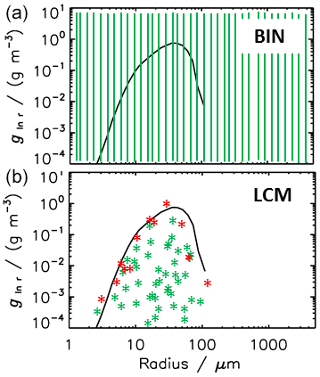
Figure 1Schematic plot of how a droplet size distribution is discretised in a bin model and represented by a SIP (simulation particle) ensemble in a Lagrangian cloud model (LCM). The red and green stars shows two different realisations of a SIP ensemble.
Using the terminology of Berry (1967), we introduce the mass density function with respect to the logarithm of droplet radius ln r:
taking into account the transformation property of distributions (fy(y)dy=fx(x(y))dx).
The DSD is usually discretised using exponentially increasing bin sizes. In analogy to U2017, the bin boundaries are defined by the masses
Note that many other studies use a factor of 21∕s for discretisation. The parameters s and κ are related via .
In an LCM, real droplets are represented by simulation particles (SIPs, also called super-droplets). Each SIP has a discrete position (vertical coordinate zp in our column model applications) and represents νp identical real droplets with an individual droplet mass μp. The total droplet mass in a SIP is then νpμp. In conjunction with SIPs, we define that the terms “low” and “high” relate to the SIP vertical position, whereas “small” and “large” relate to the droplet mass μp. The number of SIPs in a GB is defined as NSIP,GB and the total SIP number is given by .
The moments λl of order l in a GB are computed via a simple summation:
Here and in the following, index p refers to any single bin or SIP. If we want to stress that the combination of two SIPs or bins matters, we use indices i and j. Index k is used for altitude and l for the order of the moments by convention.
How does one represent an ensemble of droplets in an Eulerian or Lagrangian cloud model? Their size distribution can be uniquely described in a bin model by simply accounting for each real droplet in its respective bin, where its boundaries are given by the bin model (see illustration in Fig. 1a). In the Lagrangian approach, however, the weighting factor νi and the droplet mass μi can be chosen independently. Accordingly, there is no unique SIP representation of an ensemble of real droplets; two possible SIP ensemble realisations are illustrated in Fig. 1b.
Various techniques to generate a SIP ensemble in an LCM for a given (analytically prescribed) DSD exist (see Sect. 2.1 in U2017). In this study, we use a SIP initialisation technique (termed “singleSIP-init” in U2017), for which Lagrangian collection algorithms, and in particular AON, achieved the best results in box model tests. In the singleSIP-init, the DSD, more specifically fm, is discretised in exponentially increasing mass intervals, and a single SIP is generated for each bin (see Sect. 2.1.1 in U2017 for details). The SIP weight is given by
where μp is chosen randomly from the interval . The generation of SIPs with νp below some threshold is discarded. Due to the probabilistic component, different realisations of SIP ensembles can be created for the same prescribed DSD, and yet the initialisation technique guarantees that the moments λl,SIP are close to λl,anal. The number of generated SIPs depends on the width of the mass bins and hence on κ, as well as the other parameters of the prescribed DSD. A change of the “system size” ΔV does not change the number of SIPs but simply leads to a rescaling of the SIP weights νi. For the exponential DSD given above, around
SIPs are initialised (the scaling factor depends on the width of DSD and the choice of the lower cut-off threshold). Finally note that if the DSD is prescribed in a specific GB, the position zp of each SIP in this GB is randomly chosen from . Furthermore, δt and δV of the conceptual model take the values Δt and ΔV in the numerical models.
2.2 Eulerian column model
Eulerian column models have been widely employed in cloud physics, and the present bin implementation is conceptually similar to previous ones (e.g. Prat and Barros, 2007; Stevens and Seifert, 2008; Hu and Srivastava, 1995). We use exponentially increasing bin sizes as defined in Eq. (13). The smallest mass mbb,0 is chosen to be suitably small (corresponding roughly to a droplet radius of 1 µm), and the grid resolution parameter s sufficiently large (4 by default); i.e. the mass doubles every four bins.
The variable will be discretised in mass space and used as a prognostic variable. The droplet mass concentration in each bin p and height k is given by and approximates . For each GB k, Bott's exponential flux method (Bott, 1998, 2000) is used to solve the Smoluchowski equation. Bott's method is a one-moment scheme and gln m is the only prognostic variable. Alternatively, the collection algorithm by Wang et al. (2007) is employed, which additionally employs a prognostic equation for the droplet number concentrations in each bin.
In a second step, the mass concentrations are advected vertically according to the classical advection equation
For its numerical solution, two different positive definite advection algorithms have been used. The first option is the classical first-order upwind scheme (known for its inherent numerical diffusivity). For wsed≥0, it is simply given by
The above equation is solved independently for each bin p, where wsed is evaluated at the arithmetic bin centre . 1 A second option is the popular MPDATA algorithm, which is an iterative solver based on the upwind scheme and yet drastically reduces its diffusivity (Smolarkiewicz, 1984, 2006). By default, the basic MPDATA with two passes is employed as described in Sect. 2.1 of Smolarkiewicz and Margolin (1998).
Irrespective of the chosen advection solver, the prediction of the “new” gp,k depends on gp,k and (i.e. the GB above the one of interest). For the prediction of at the model top, it is necessary to prescribe the value , which defines the upper boundary condition (this is detailed in Sect. 2.4).
If the prescribed Δt is too large and the Courant–Friedrichs–Levy (CFL) criterion is violated, sub-cycling is introduced. As does not change over the course of a simulation, the (bin-dependent) number of subcycles nsubc,p is determined in the beginning, such that rCFL=0.5 holds for the reduced time step .
After one call of Bott's algorithm, nsubc,p calls of the selected advection algorithm with reduced time step follow for each bin p.
The moments are computed by
as given in Eq. (48) of Wang et al. (2007), where is the geometric bin centre.
2.3 Lagrangian column model
In a Lagrangian model, the inclusion of sedimentation (obeying the transport equation ) is straightforward. For each SIP the particle position is updated via
Unlike in Eulerian methods, sedimentation in a Lagrangian approach is independent of the chosen mesh, and the time step is not restricted by numerical reasons. If zp becomes negative at some point in time, the SIP crossed the lower boundary and is removed.
For the collection process, it assumed that each SIP belongs to a certain GB k obeying and that the real droplets of each SIP are well-mixed in the GB volume (WM3D). The collection process is treated with the probabilistic AON algorithm. In the regular version (see Sect. 2.3.1), AON is called for each GB and accounts for all possible collisions among any two SIPs of the same GB. By construction, the information on the vertical position is irrelevant inside the regular AON and is only used in the SIP-to-GB assignment.
In the version with explicit overtakes (WM2D; see Sect. 2.3.2), for any two SIPs (of the whole column) it is checked if the higher SIP (i.e. with larger zp) overtakes the lower SIP within the current time step. This may have several advantages: First, only 2D well-mixedness in a horizontal plane is assumed and possible size sorting effects within a GB are accounted for. Moreover, in Lagrangian methods the time step is not restricted by the CFL criterion and the largest SIPs may travel through more than one GB. In the classical approach, such a SIP can only collect SIPs from the GB where it was present in the beginning of the time step. In the second approach, collections can also occur across GB boundaries (see Sect. 2.3.2).
In the remainder of this paper, the classical approach is referred to as AON-regular and the new approach as AON-WM2D. Figure 2 sketches how the SIP properties (location, weighting factor, sedimentation speed) are interpreted in either approach. For simplicity, a single GB with one SIP pair is displayed.
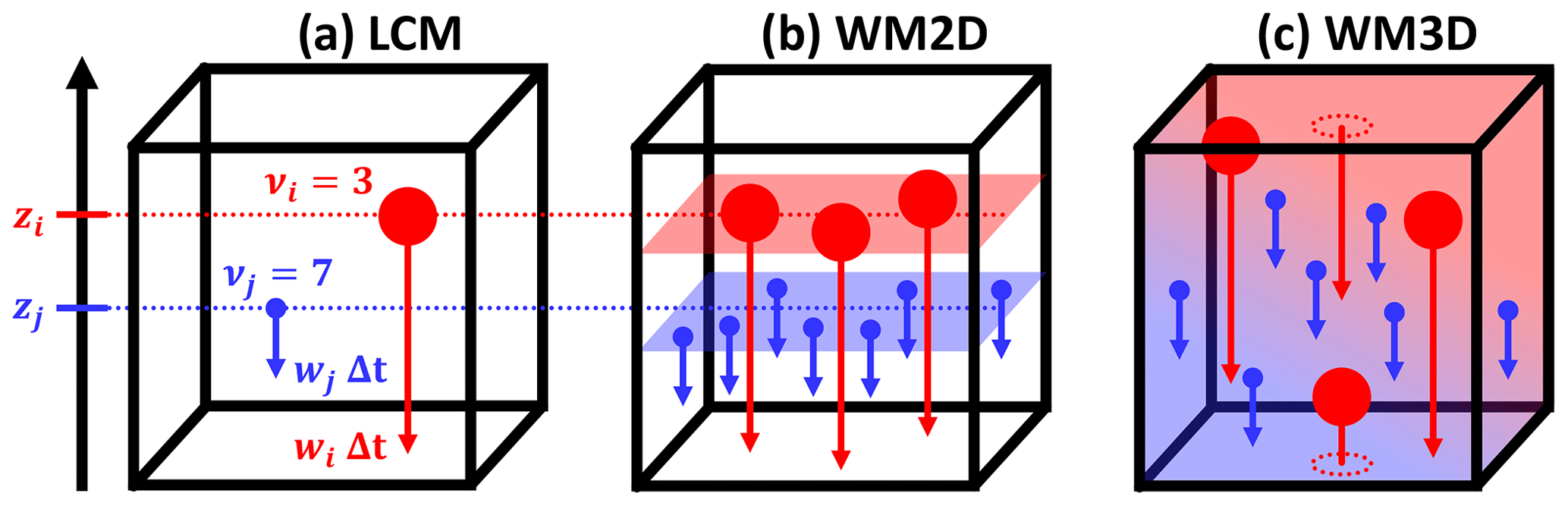
Figure 2Grid box with a SIP pair in the LCM world (a) and its respective interpretation in the 2D well-mixed (WM2D, b) and 3D well-mixed (WM3D, c) approach of the AON collisional growth algorithm.
AON is probabilistic and an individual realisation does not usually reproduce the mean state as predicted by deterministic methods like Eulerian approaches. The extent of deviations from the mean state is exemplified in Fig. 15 of U2017 for a box model application of AON. Hence, the AON results discussed in the present study are usually ensemble averages over nrinst=20 realisations.
Pseudo-code of both algorithm implementations is given. For the sake of readability, the pseudo-code examples show easy-to-understand implementations. The actual codes of the algorithms are, however, optimised in terms of computational efficiency. The style conventions for the pseudo-code examples are as follows: commands of the algorithms are written in upright font with keywords in boldface. Comments appear in italic font (explanations are enclosed by brace brackets {}, and headings of code blocks are in boldface).
2.3.1 Regular AON algorithm (AON-regular)
Here we basically repeat the AON description of U2017 (their Sect. 2.5).
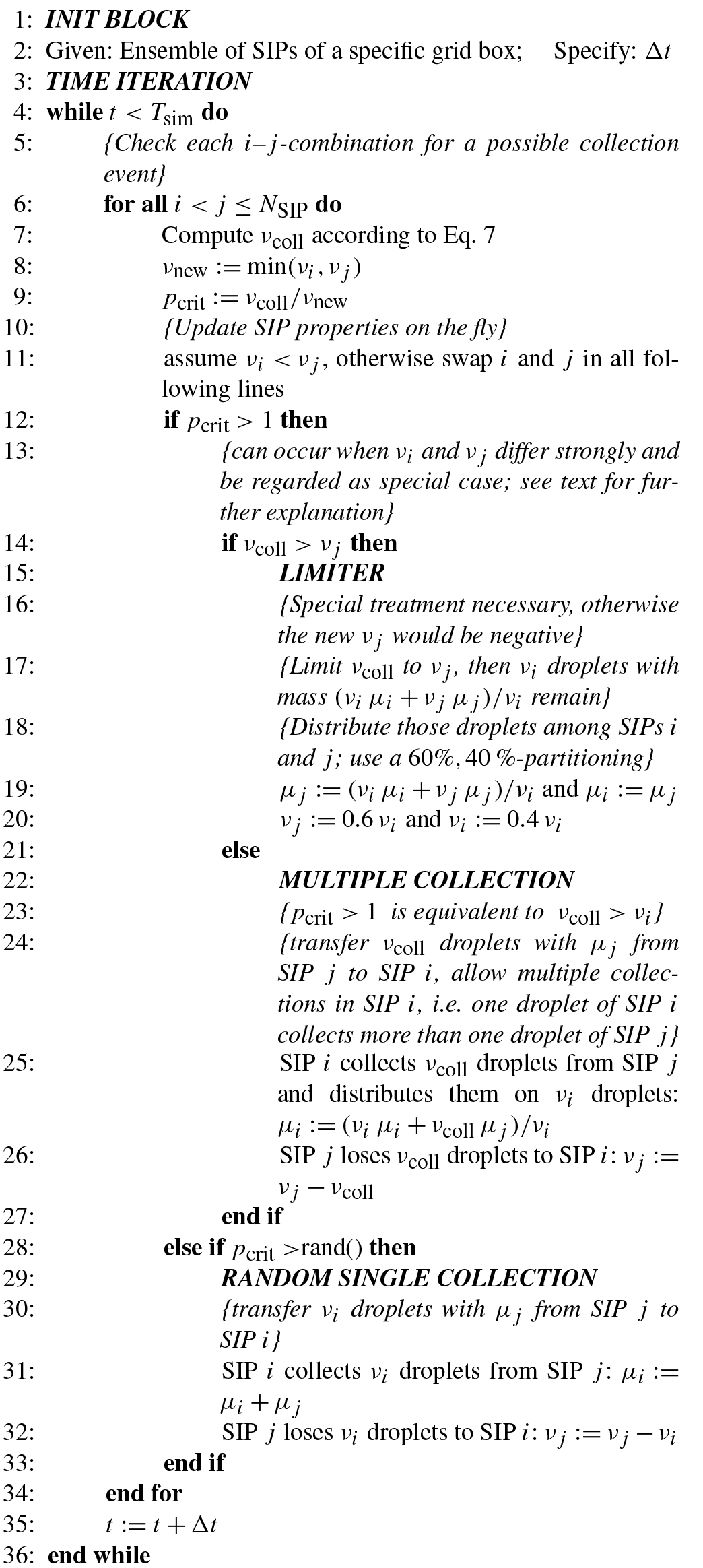
Pseudo-code of the regular all-or-nothing (AON) algorithm; style conventions are explained right before Sect. 2.3.1 starts; rand() generates uniformly distributed random numbers . This AON version is called independently for each grid box.
“Figure 3 illustrates how a collection between two SIPs is treated. SIP i is assumed to represent fewer droplets than SIP j, i.e. νi<νj. Each real droplet in SIP i collects one real droplet from SIP j. Hence, SIP i contains νi=4 droplets, now with mass . SIP j now contains droplets with mass μj=9. Following Eq. (7), only νcoll=2 pairs of droplets would, however, merge in reality. The idea behind this probabilistic AON is that such a collection event is realised only under certain circumstances in the model, namely such that the expectation values of collection events in the model and in the real world are the same. This is achieved if a collection event occurs with probability
in the model. Then, the average number of collections in the model,
is equal to νcoll as in the real world. A collection event between two SIPs occurs if pcrit > rand(). The function rand() provides uniformly distributed random numbers . Noticeably, no operation on a specific SIP pair is performed if pcrit<rand().
The treatment of the special case needs some clarification. This case is regularly encountered when SIPs with large droplets and small νi collect small droplets from a SIP with large νj. The large difference in droplet masses μ led to large kernel values and high νcoll with . […] If pcrit>1, we allow multiple collections, as each droplet in SIP i is allowed to collect more than one droplet from SIP j. In total, SIP i collects νcoll droplets from SIP j and distributes them on νi droplets. A total mass of νcollμj is transferred from SIP j to SIP i and the droplet mass in SIPs i becomes . The number of droplets in SIP j is reduced by νcoll and . Keeping with the example in Fig. 3 and assuming νcoll=5, each of the νi=4 droplets would collect droplets. The properties of SIP i and SIP j are then νi=4, μi=17.25, νj=3 and μj=9. […] So far, we explained how a single i–j combination is treated in AON. In every time step, the full algorithm simply checks each i−j combination for a possible collection event. To avoid double counting, only combinations with i<j. Pseudo-code of the algorithm is given in Algorithm (1). The SIP properties are updated on the fly. If a certain SIP is involved in a collection event in the model and changes its properties, all subsequent combinations with this SIP take into account the updated SIP properties. […] For the generation of the random numbers, the well-proven (L'Ecuyer and Simard, 2007) Mersenne Twister algorithm by Matsumoto and Nishimura (1998) is used.”
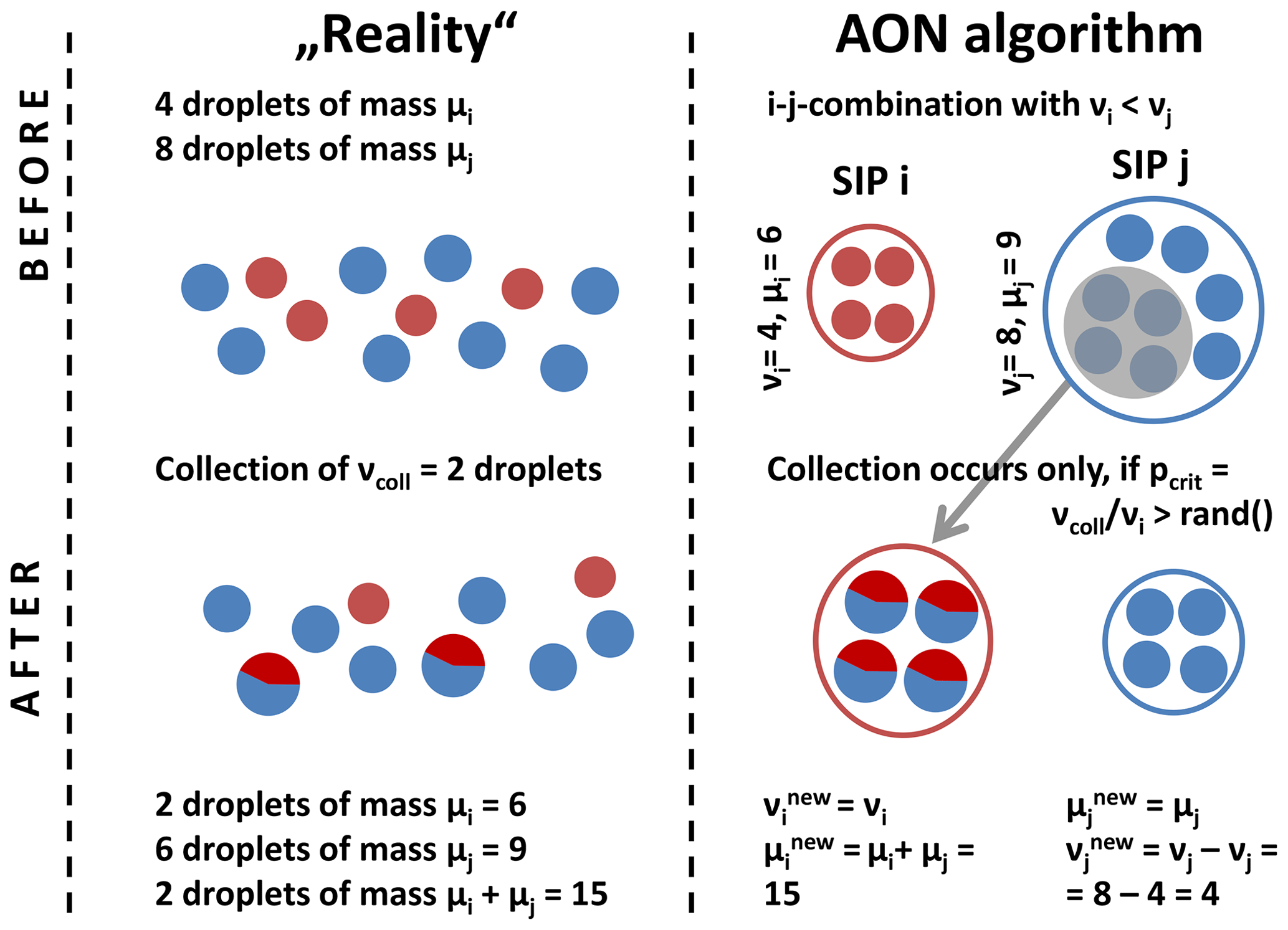
Figure 3Treatment of a collection between two SIPs in the all-or-nothing (AON) algorithm, partially adopted from Fig. 2 of Unterstrasser et al. (2017).
The AON treatment of collection of droplets within one SIP, as well as the collection of two SIPs with equal weighting factors, is described in U2017. In the simulations presented here these aspects are not relevant and thus omitted.
The current implementation differs in several aspects from the version in Shima et al. (2009). First, they use a linear sampling approach (which will be described in Sect. 2.3.3). Second, the weighting factors are considered to be integer numbers, whereas we use real numbers ν. Integer values are appropriate in discrete test cases of small sample volumes such as the validation test case in Sect. 3 of Dziekan and Pawlowska (2017). For comparing AON with bin model references, usually continuous DSDs are prescribed. Then a SIP ensemble with real-value weighting factors is more appropriate in our opinion. Third, multiple collections (MCs) are differently treated. For , either ⌊pcrit⌋νi or ⌈pcrit⌉νi droplets of SIP j merge with νi droplets of SIP i depending on the probability pcrit−⌊pcrit⌋. This maintains the integer property of the SIP weights. As the latter feature is not required in our approach, we deterministically merge pcritνi=νcoll droplets from SIP j with νi droplets of SIP i. This is computationally more efficient than the integer-preserving implementation. Test simulations showed that both MC treatments produce similar results.
2.3.2 AON algorithm with explicit use of vertical coordinate (AON-WM2D)
Pseudo-code of the AON-WM2D algorithm; style conventions are explained right before Sect. 2.3.1 starts; rand() generates uniformly distributed random numbers . This AON version is called once for the total column.
We now introduce the AON version based on an idea by Sölch and Kärcher (2010) where the vertical position zp of the SIPs is explicitly considered. The approach and its implications will be detailed next. Pseudo-code of this AON version (“WM2D”) is given in Algorithm Pseudo-code of the AON-WM2D algorithm; style conventions are explained right before Sect. starts; rand() generates uniformly distributed random numbers ∈[0,1). This AON version is called once for the total column..
Unlike the classical case where 3D well-mixedness has to be assumed, droplets of a SIP are now assumed to be well-mixed on the x–y plane at z=zp within the GB (horizontally well-mixed instead of the traditional well-mixed assumption for the entire three-dimensional GB) and represent a “concentration” of (units L−2, where L is a length scale). We introduce an adapted kernel definition where the relative velocity term is dropped from Eq. (5):
The AON algorithm is split into two steps:
-
Based on the evaluation of the vertical positions zi and zj at times t and t+Δt, a check is made to see if SIP i overtakes SIP j within a time step Δt. Given zi(t)≥zj(t) (otherwise swap i and j) an overtake takes place in the time interval Δt if .
-
In case of such an overtake: compute the average number of droplet collections by
Analogous to the classical implementation, a collection in the model is performed with a probability νcoll∕νi and SIP i may collect νi from SIP j (in this step i and j are chosen such that νi<νj).
Similarly to the WM3D version, it happens that νcoll is larger than νi, and multiple collections are also considered in AON-WM2D.
Specifically to WM2D, it is also possible that a SIP interacts with other SIPs located in not only one but several GBs. Accordingly, it is not only necessary to check overtakes of other SIPs in the original GB (more specifically, SIPs that lie in the same GB at time t), but also the SIPs that are located underneath, depending on the prescribed time step.
In a Lagrangian model, the time step choice is not numerically restricted by the CFL criterion and in particular the largest collecting drops may fall through several GBs during the time period Δt. Hence, their collections are underrated unless potential overtakes are checked among all NSIP,tot SIPs of the entire column. Even if the CFL criterion is obeyed, SIPs close to the lower GB boundary will mostly collect SIPs from the GB underneath. Hence, seeking collision candidates only in the present GB is never a good choice.
In a naive implementation, this would dramatically increase the computational costs. In the regular (WM3D) version, nz calls of AON with (for simplicity lets assume NSIP,GB is the same in all GBs) give a total cost of . Contrarily, AON-WM2D is called once for all SIPs of the column. Hence the cost is and a factor nz higher than the regular AON version. However, the WM2D version can be sped up by first sorting all SIPs by their position (if sorting is done independently in each GB, the complexity is nz×𝒪(NSIP,GBlog (NSIP,GB))), and second by taking into account that the final position zi(t+Δt) of the potentially overtaking SIP i must be below the initial position zj(t) of SIP j. Finding possible candidates for SIP i within the sorted SIP list can be stopped once a SIP j with is encountered (see condition in line 10 of Algorithm Pseudo-code of the AON-WM2D algorithm; style conventions are explained right before Sect. starts; rand() generates uniformly distributed random numbers ∈[0,1). This AON version is called once for the total column.).
For the smallest SIPs, which often travel only a small distance inside a GB, the list of SIPs that may be overtaken is commensurately small and overtakes have to be checked for a fraction of SIPs of the GB only (that means the actual computational work is smaller than in the regular version). On the other hand, imagine the largest SIPs travel through three GBs – then overtakes have to be tested for roughly 3 times more SIPs than in the regular version. Moreover, testing for overtakes (step 1) is computationally less demanding than calculating the potential collections (step 2). In WM3D we always have the workload of step 2 for all tested combinations, whereas in WM2D only the cheaper step 1 is executed in case of no overtake.
Besides the weaker assumption of 2D well-mixedness, the present approach is actually more intuitive (even though it may first be regarded counter-intuitive by those who are familiar with traditional Eulerian grid-based approaches). Moreover, this approach complies better with the Lagrangian paradigm of a grid-free description (the present approach is independent of nz and Δz, and yet some horizontal “mixing area” ΔA has to defined, over which the droplets of a SIP are assumed to be dispersed). In the regular AON, the aspect ratios of the grid box do not matter, and only the grid box volume ΔV enters the computations. In WM2D, on the other hand, the value of ΔV is insignificant, and ΔA enters the computations. In a column model with sedimentation, results also depend on Δz as it determines the travel time through a grid box. Note that a variation of Δz can also implicitly change ΔV or ΔA.
For more sophisticated kernels, including for example turbulence enhancement, the present approach may not be adopted easily as the driving mechanism for collisions to occur in the current model is differential sedimentation. Related to this are studies on cylindrical vs. spherical formulations of kernels in Saffman and Turner (1956) and Wang et al. (1998, 2005). A possible route to consider the effects of sub-grid motions on collision in LCMs has recently been presented by Krueger and Kerstein (2018). Their one-dimensional approach is able to represent droplet clustering and turbulence-induced relative droplet velocities in a realistic manner, and its implementation in already applied LCM sub-grid-scale models (e.g. Hoffmann et al., 2019; Hoffmann and Feingold, 2019) is deemed straightforward. However, further research is required on how the limited number of SIPs in current LCM applications may corrupt the correct representation of such processes.
Finally, we briefly summarise the differences between the WM2D and WM3D approach. The standard kernel KWM3D as given by Eq. (5) has units L3∕T (where L and T are a length scale and timescale, resp.). Multiplying it by concentrations ni and nj (units L−3), one obtains the rate of a concentration increase in merged droplets () which is finally multiplied by δt (unit T) to obtain ncoll (see Eq. 8). Since SIPs represent droplet concentrations of and , Eq. (7) follows. In the WM2D approach, the kernel KWM2D as given by Eq. (23) has units L2. Multiplying it by “2D” concentrations n2D,i and n2D,j (units L−2) one obtains the collected 2D concentration n2D,coll (units L−2). Since SIPs represent “2D” droplet concentrations of and , Eq. (24) follows. A collection can only occur if a larger droplet (or SIP) i overtakes a smaller droplet (or SIP) j. First, zi>zj and must hold and second the overtake time must fulfil ΔtOT≤δt. One can define the overtake probability pOT being 0 for ΔtOT>δt and 1 for ΔtOT≤δt, and the “2D” collection probability . Simulations in the Supplement demonstrate that the WM2D and WM3D formulations are statistically equivalent; i.e. pOT×pWM2D equals pWM3D, under certain conditions (see Fig. S9).
From a technical point of view, it might be challenging to implement the WM2D version in full 2D/3D cloud models, as one has to keep track of all SIPs in a grid box column. If domain decomposition is used in a vertical direction, collision candidates had to be searched across multiple processors.
2.3.3 Linear sampling version (AON-LinSamp)
The regular AON version can be sped up by introducing a linear sampling technique (LinSamp) as done in Shima et al. (2009) or Dziekan and Pawlowska (2017). ⌊NSIP∕2⌋ combinations of pairs i−j are randomly picked, where each SIP appears in exactly one pair (if NSIP is odd, one SIP is ignored). As only a subset of all possible combinations is numerically evaluated, the extent of collisions is underestimated. To compensate for this, the probability pcrit (or equivalently νcoll) is upscaled by a scaling factor
to guarantee an expectation value as desired. Clearly, this reduces the computational complexity of the algorithm from to 𝒪(NSIP). Multiple collections are more likely than in the regular AON version. The LinSamp version becomes the preferred choice if NSIP is large.
If νcoll is larger than both νi and νj, all AON versions as introduced so far would produce negative weights. In order to prevent this, νcoll is artificially reduced to νj in such a case (let us assume that νi<νj). The standard procedure would then produce a SIP j with zero weight, which allows the updated SIP i with weight νi (the weight νi remains unchanged during the update) to be split into two SIPs. We choose a 60 %–40 % partitioning, and the operations are as follows.
The Supplement demonstrates that how the limiter is implemented is critical. We thank reviewer Shin-ichiro Shima for pointing us to a better limiter implementation, which has been already described in Shima et al. (2009). There, a 50 %–50 % partitioning was implemented. We avoid this equal splitting as it produces two identical SIPs. In our implementation with floating point weights, SIPs with identical weights are extremely rare and no special care is taken for this. Hence, including an operation that produces identical weights is unfavourable. The dependence of the AON-LinSamp performance on the limiter definition is showcased in the Supplement (Figs. S3–S7, S15 and S16 and Table S1).
Employing a limiter is recommended for all AON versions (even though we never encountered a limiter event in QuadSamp simulations), but it is particularly significant in the LinSamp version due to the upscaling of pcrit. Moreover, note that LinSamp can be reasonably used only in conjunction with AON-WM3D, not AON-WM2D.
In addition to the favourable linear computational complexity, LinSamp can be easily parallelised, in particular on shared-memory multi-processor architectures as used by Arabas et al. (2015) or Dziekan et al. (2019). Once the SIP pairs are determined in the beginning of each time step, each processor treats a subset of SIP pairs. After a collection event, SIP properties are updated on the fly. Note that the need to do updates on the fly precludes simple parallelisation strategies in the quadratic sampling version, where all SIPs are interconnected.
2.4 Boundary condition
At the lower boundary, droplets leave the domain according to their fall speed. Using the LCM, the moment outflow Fl,out is determined by accumulating the contributions νp(μp)l of all SIPs p that cross the lower boundary z=0 m. Due to the discreteness of the crossings, instantaneous fluxes are actually averages of the past 200 s. Using the bin model, Fl,out is diagnosed by
At the model top, the simplest condition is to have a zero influx. In this case, the column-integrated droplet mass will decrease once a non-zero flux across the lower boundary occurs. To implement a zero-influx condition in the Eulerian model, the mass concentrations at the ghost cell level nz+1 are simply set to zero. In the Lagrangian model, a zero influx condition is naturally implemented when no new SIPs are created at the top of the column.
In both models, a non-zero influx at the model top can also be prescribed. One option is to use periodic boundary conditions. In the Lagrangian approach this is done by increasing the altitude zp of an affected SIP by Lz, once zp drops below 0. In the Eulerian model, is identified with gp,1. A second non-zero influx option is a prescribed size distribution that is advected into the domain with its respective fall speed. In the bin model, the prescribed DSD simply defines the values. In the Lagrangian model, new SIPs have to be introduced close to the model top. For this, a new SIP ensemble is drawn from the prescribed DSD at each time step using the SingleSIP-init method. In order to place the SIPs in the column, the greatest distance it would fall from the model top during one time step is considered: . In a straightforward implementation, one would create one SIP from each bin with a position znew,p uniformly drawn from and weighting factor . This implementation has, however, several undesirable side effects. For small, slowly falling SIPs zΔ(p) is much smaller than Δz. Applying this procedure in every time step leads to Δz∕zΔ(p) SIPs per GB in the end. Hence, we refine this procedure by creating a SIP with probability , a weighting factor νnew,p=νp and . Note that if , then either ⌊pinit,p⌋ or ⌈pinit,p⌉ SIPs are created depending on the probability . This establishes a similar spatial SIP occurrence across the size spectrum with one SIP per GB and bin on average. Moreover, SIP numbers do not scale any longer with Δt.

2.5 Terminology
Before we start discussing the results, we outline the terminology of the various model versions. On a first level, we differentiate between Eulerian (“BIN”) and Lagrangian approaches (“LCM”), which can be both applied in a box (“0D”) or column model (“1D”) framework. By default, BIN uses the MPDATA advection algorithm (clearly only in 1D) and Bott's collection algorithm. Alternatively, MPDATA can be replaced by the first-order upstream scheme (“US1”) and Bott's collection algorithm by Wang's algorithm (“Wang”). The Lagrangian model versions differ only in the way AON is employed. The various model versions are summarised in Table 2. By default, 3D well-mixedness (“WM3D”) is assumed and a quadratic sampling (“QuadSamp”) of the SIP combinations is used. Those simulations are referred to as “regular”. A second type of QuadSamp simulation assumes 2D well-mixedness (“WM2D”). Linear sampling of SIP combinations (“LinSamp”) can be alternatively used for the WM3D version. Accordingly, the terms “regular”, “WM2D” and “LinSamp” each refer to one specific AON version. On the other hand, “QuadSamp” and “WM3D” each denote two AON versions: “QuadSamp” comprises “regular” and “WM2D”, whereas “WM3D” comprises “regular” and “LinSamp”.
By switching off sedimentation in the column model source code (as partially done in Sect. 3.1), box model results are produced in each GB. In order to distinguish the latter simulations from AON box model results in U2017 they are referred to as “noSedi”. In LCM1D-noSedi simulations, the vertical position is not updated from time step to time step. Hence, this implicitly calls for the usage of AON-WM3D, as AON-WM2D relies on checking overtakes based on the vertical SIP positions. Simulations with switched-on sedimentation are the default; for better discrimination from the noSedi case we refer to all such simulations optionally as “full” simulations.
If the space in figure legends is limited, abbreviations “LS” and “nS” are used for “LinSamp” and “noSedi”, respectively.
Before we start comparing collisional growth in column model applications, we should first demonstrate that the differences introduced by the different numerical treatment of the sedimentation process are small to negligible. This exercises is deferred to the Appendix.
We find the discrepancies introduced by the different sedimentation treatments small enough as long as the MPDATA advection algorithm is employed in BIN. Hence, all following BIN simulations rely on MPDATA and we can attribute the differences that we may see in the following validation exercises to the different numerical treatment of collisional growth.
3.1 Box model emulation simulations
In this section, we choose a column model set-up that is supposed to produce results that are similar to box model results. For this, we initialise the default DSD in all GBs of the column and use periodic boundary conditions. In LCM1D, different SIP ensemble realisations of this DSD are initialised in each GB.
The deterministic BIN1D model predicts identical DSDs in all GBs, as in each GB the divergence of the sedimentation flux is zero. Hence, for this specific set-up, the BIN1D results attained are identical to those of a corresponding BIN0D model or the data of Wang et al. (2007, see their Tables 3 and 4).
In LCM1D, the combination of homogeneous initial conditions and periodic BCs results in statistically identical results across all GBs. However, the averaged results may not be the same as in LCM0D, as lucky droplets or SIPs (Telford, 1955; Kostinski and Shaw, 2005) can collect other droplets or SIPs not only from a single GB as in LCM0D, but from any GB (depending on how fast they fall), creating potentially larger and/or faster-growing lucky droplets/SIPs than in LCM0D. In other words, the number of SIPs interacting with each other is increased in LCM1D. This, as we will show below, accelerates the convergence of the simulations.
Within the LCM1D model, pure box model results can be obtained by switching off sedimentation (“noSedi”). Without sedimentation, the GBs of the column are not interconnected and the collisional growth process proceeds independently.
All figures related to the box model emulation set-up start their caption with the label “BoxModelEmul set-up”.
By default, we use nz=50 GBs with Δz=10 m (giving a column height of Lz=500 m), ΔV=1 m3, Δt=10 s and κ=40 throughout Sect. 3.1. The results are averaged over nrinst=20 independent realisations. Hence, the present AON application can be viewed as a Monte Carlo method.
Moreover, we use the Long kernel (Long, 1974) as default in BoxModelEmul simulations, as U2017 revealed that numerical convergence is harder to reach for the Long kernel than for the Hall kernel or a hydrodynamic kernel with constant aggregation efficiency typically used for cirrus simulations (Sölch and Kärcher, 2010).
3.1.1 Regular AON version
This subsection presents results obtained with the regular AON, i.e. with quadratic sampling of SIP combinations (“QuadSamp”) and 3D well-mixed assumption (WM3D). Sedimentation is switched on unless noted (for better discrimination from the “noSedi” cases, these simulations will be referred to as “full”).

Figure 4BoxModelEmul set-up: temporal evolution of column-averaged moments λ0 and λ2 over 1 h for various time steps Δt (see inserted legend for Δt values) for the regular AON version. All other parameters take the default values as given in the caption of Fig. 5.

Figure 5BoxModelEmul set-up: temporal evolution of column-averaged moment λ0 (i.e. droplet concentration) over 1 h for the regular AON version. The default setting is nz=50, nrinst=20, ΔV=1 m3, Δt=10 s, Δz=10 m, κ=40 and . The microphysical parameters of the initial exponential droplet size distribution are LWCinit=1 g m−3, rinit=9.3 µm and DNCinit=297 cm−3 as in many previous studies (Berry, 1967; Wang et al., 2007). The parameter or parameter pair that is varied is added in a purple box to each panel and the legend lists the parameter values for the different colours. If further parameters (besides the varied parameter) take non-default values, it is indicated inside a black rectangle. In any case, the total number of GBs is . By default, sedimentation is switched on. Simulations without sedimentation and independent rain formation in each GB (identical to a box model treatment) are labelled as “noSedi” (appear only in the left column). The panels on the right use a shortened time range.
Figure 4 shows the temporal evolution of column-averaged LCM1D moments λl (l=0 and 2) over 1 h for various time steps Δt. The box model data serve as orientation in this and following Figs. 5–7. We find that in terms of λ0 and λ2 LCM1D results converge for Δt≤10 s. The noSedi simulations show a similar time step dependence (not shown). Hence, AON works well even for large time steps, a fact that was already shown with the AON box model (see Fig. 18 of U2017).
Next, we discuss the sensitivity to further physical and numerical parameters. Generally, we find faster convergence for higher moments than for λ0 (not shown). Hence in the following, we confine our analysis to the most “critical” quantity, and Fig. 5 displays the λ0 evolution for various sensitivity experiments. Even though we analyse the results in some detail, we want to mention that the observed differences are in principle not substantial. In fact, results differ much more due to a different collection kernel or slightly varied initial DSDs (see Sect. 3.1.4). Nevertheless, the analysis will help to understand more deeply how collisional growth works in an LCM with AON. This pronounced effort is justified, as precipitation initiation is still not fully understood and a well-validated Lagrangian approach may lead to new insights (Dziekan and Pawlowska, 2017; Grabowski et al., 2019).
In a first simple step, we vary nz (see Fig. 5a and b), which changes two aspects of the numerical set-up: the number of GBs over which interactions can occur and the height of the column. This implicitly changes the time it takes for SIPs to fall through the total column and hence changes the ”recycling” timescale Lz∕wsed. Together with nz, nrinst is varied such that nz×nrinst is always 1000. Accordingly, all simulation results are averaged over the same number of GBs, and we avoid cases of simulations with smaller nz producing noisier data.
In the noSedi simulations (panel a), the moment evolution is not affected by varying (nz, nrinst). This is trivial, as in any case the average is taken over 1000 independent GBs. At least, these results demonstrate that averaging over that many GBs suffices by far to produce robust averages. In the full simulations (panel b), the λ0 decrease is more pronounced, and the various set-ups produce nearly identical results (except for the case with nz=2, which is in between the other full simulations and the noSedi simulations). From this finding alone one may argue that the collisional growth process is more efficient in LCM1D than in LCM0D.
The second row shows a variation of κ which reveals qualitatively different convergence properties of the noSedi simulations (panel c) and the full simulations (panel d). In the noSedi simulations, an increase in κ (and NSIP; see extra legend for corresponding NSIP values) leads to a faster decrease in λ0. Large differences between κ=5 and κ=40 simulations are apparent; above κ=40, an increase in κ leads only to marginal improvements. Also, for the highest κ, the λ0 values remain above the BIN0D reference. For the smallest κ value, only 24 SIPs are created according to Eq. (16), and interactions among those few computational particles overemphasise the impact of correlations. It is well-known that for small ensembles of real droplets correlations become important (Bayewitz et al., 1974; Wang et al., 2006). Analogously, we introduced correlations in our numerical approach by using too few computational particles. We speculate that this hinders the formation of lucky droplets and fewer droplets get collected (hence λ0 is larger for smaller κ). Another more technical explanation is that the νp distribution of the SIP ensemble is such that the formation of lucky SIPs is not supported. Ideally, there is a reservoir of SIPs with small ν values that can become lucky SIPs. There might be too few SIPs with small ν for small κ.
Contrarily, the full simulations (panel d) give nearly identical results independent of κ. We obtain converged results with as few as 24 SIPs in each GB. Compared to κ=200 with 1000 SIPs, the simulations are a factor of 402 faster. The reason for the much faster convergence in terms of NSIP,GB is that the GBs are interconnected, which effectively raises the number of potential collision partners. Drops with radii of 100 and 500 µm have fall speeds of around 0.7 and 4 m s−1, respectively. Thus it takes them around 14 and 2.5 s to fall through a Δz=10 m GB and they enter a new GB every time step or every few time steps given Δt=10 s.
How strongly SIPs are interconnected across GBs in LCM1D should also depend on geometrical properties of the column. In the next set-up, we investigate the κ sensitivity in a column with nz=10 and Δz=100 m instead of nz=50 and Δz=10 m (panel e). Then, SIP interactions can occur only across 10 GBs, and overall 5 times fewer SIPs are present in the column than for the default case with nz=50. Moreover, the domain is stretched by increasing Δz to 100 m, which increases the residence time of a SIP in a GB by a factor of 10, additionally slowing down SIP interactions across GBs. Those two changes introduce a weak κ dependence, and yet it is much weaker than in the corresponding noSedi simulations (panel c).
In an even more academic experiment, sedimentation is turned off, but SIPs are randomly redistributed inside the column after each time step (panel f) similar to Schwenkel et al. (2018). Again, we find converged results for small κ values as small as 5 (panel f). This elucidates that convergence is improved once some process exchanges SIPs between GBs, be it for physical reasons like sedimentation or by an artificial operation such as the randomised SIP re-location. We speculate that in full 2D/3D LCM simulations turbulent motions and sedimentation increase the SIP exchange across GBs and hence may additionally increase the performance of AON. The two last simulation series are promising, as they suggest that in a column model (and probably also 2D or 3D models) convergence is potentially reached with fewer SIPs per GB than in a box model. Nevertheless the tests also highlight that convergence with κ depends on many circumstances and convergence tests are a prerequisite to any LCM simulation with AON.
In bin models, the Smoluchowski equation, which is strictly valid only for an infinite volume and hence an infinite number of well-mixed droplets, is solved. Accordingly, only concentrations are prescribed in bin model algorithms. Neither ΔV nor the absolute number of droplets is considered in this approach. At least in the limit of all SIPs having weighting factor ν=1, the AON algorithm solves the master equation (Dziekan and Pawlowska, 2017), which takes into account ΔV, and results may depend on the actual number of involved droplets. Clearly, correlations (which are accounted for in the master equation) are larger in smaller volumes (Bayewitz et al., 1974; Wang et al., 2006; Alfonso and Raga, 2017).
For our SIP-initialisation procedure, NSIP,GB depends solely on the chosen κ values and is independent of ΔV. By construction, a ΔV variation does not affect at all the simulation results, as all SIP weights are simply rescaled. Indeed, we obtain nearly bit-identical results for a ΔV variation. To explore the ΔV sensitivity in our LCM1D, the SIP-init procedure has to be adapted. In the adapted version the SIP number increases proportionally with ΔV as it would in reality. As computational requirements increase quadratically with NSIP,GB, the variation of ΔV and NSIP,GB can be performed only for a small range of ΔV values. ΔV is increased by a factor of 5 or 10. As a base case, we use the simulations with κ=20 and κ=100 and define ΔV:=1 m3. The fourth row shows results for the noSedi (panel g) and the full simulations (panel h). Apparently, the noSedi simulations with larger ΔV converge to the solution we obtained before by using a sufficiently large κ. In full simulations, a ΔV variation has basically no effect. The κ=100, ΔV=10 m3 simulation considered on average collisions between 5000 SIPs in each GB. Yet, the results are basically identical to the case κ=5, ΔV=1 m3 with 24 SIPs in each GB (which runs nearly 40 000 times faster).
In the present simulations, where SIPs with weights ν>1 are used, variations of the numerical parameter κ and the physical parameter ΔV are interconnected and their effects cannot be disentangled. Hence, the AON algorithm can only answer whether correlations matter in systems with a certain number of SIPs. These correlations are not necessarily the correlations one would see in a real system with millions to billions of real droplets. Nevertheless, the last sensitivity series implies that at least in our model system the importance of correlations is likely the same as in a system with NSIP,GB=24 and with NSIP,GB≈5000. Assuming that the importance of correlations in a real system with billions of droplets is similar to that of a system with 5000 SIPs, the latter finding demonstrates that LCMs can capture the collisional growth process with astonishingly few SIPs.
The noSedi κ sensitivity series as shown in panel (c) was already presented in Fig. 18 of U2017. There we found that for high enough κ the LCM0D results lie below the BIN0D reference contradictory to the present noSedi simulations. The reason for this inconsistency is a programming bug in the LCM0D-AON version used in U2017. The Hall and Long kernel values are stored in look-up tables and were wrongly accessed (overestimating the actual mass of the involved droplets by 2 %). Hence, the collisional growth process proceeded more rapidly in U2017. Despite this flaw, the main findings of U2017 remain valid. Yet, the more rapid collisional growth of LCM0D-AON in U2017 should clearly not be attributed to conceptual differences of AON and BIN algorithms.
In the discussion of the subsequent sensitivity studies, we refrain from showing time series of λ0 as done in Fig. 5. Instead we only evaluate λ0 at t=1 h as this is a suitable metric for the algorithm performance in the BoxModelEmul set-up. Figure 6 comprises Δt and κ sensitivity series of all subsequent BoxModelEmul simulations. The black dotted (horizontal) line depicts the reference BIN result obtained with Wang's algorithm with s=16 and Δt=1 s and was already added in Fig. 5 for orientation.

Figure 6BoxModelEmul set-up: this figure summarises results of many sensitivity studies for various AON versions and BIN simulations by displaying DNC after 1 h as a function of resolution κ (or analogously s in BIN models) or time step Δt. The default parameter settings are listed in Fig. 5 and the horizontal black dotted curve shows the BIN benchmark reference. For example, the information of Fig. 5c and d is compressed into the two grey curves in panel (a). Panels (a) and (b) additionally show AON simulations with linear sampling (as described in Sect. 2.3.3), unless “reg” in the legend indicates regular AON with quadratic sampling. “nS” is short for “NoSedi”. The second row shows simulations with explicit overtakes and a 2D well-mixed assumption (“WM2D”, as described in Sect. 2.3.2). Again, the regular AON with WM3D serves as reference. In the simulation labelled “WM2D(GB)”, overtakes are considered only between SIPs inside the same GB, whereas “WM2D” checks overtakes in the full column. Panel (e) shows a scenario with (increased) LWCinit=1.5 g m−3 and (f) uses the Hall kernel instead of the Long kernel. Note that the y ranges are different in the third row. The fourth row shows BIN results with Bott's and Wang's algorithms. The default parameters are s=4 and Δt=10 s.
3.1.2 AON with linear sampling
This subsection discusses the AON version with linear sampling. Both full simulations and noSedi simulations have been carried out. The first row of Fig. 6 shows sensitivity of λ0(t=1 h) to κ (a) and Δt (b), respectively. The grey curves repeat the regular AON results (i.e. with quadratic sampling); they show the endpoints of curves shown in Fig. 4 (top) and Fig. 5c and d. We find that the qualitative behaviour does not differ between LinSamp and regular AON.
In the full simulations (solid lines), simulations converge for any κ, whereas for the noSedi simulations (dotted, “nS” in the legend) convergence is reached only for the largest κ values. Using the default time step Δt=10 s, the LinSamp results (orange curves) are slightly further away from the BIN reference (black dots) than the regular results. A second LinSamp series with Δt=1 s (blue) produces better results than the regular AON version with Δt=10 s.
The Δt sensitivity series shown in the right panels of Fig. 6 demonstrates that LinSamp results are slightly worse than the regular results for the default resolution κ=40. Using LinSamp with a finer resolution of κ=100 produces better results than the regular AON with κ=40. In LinSamp simulations with large time steps, limiter cases occur quite often and one may expect that the artificial reduction of collection events strongly deteriorates the model outcome. However, we see that the performance in the high-Δt range drops similarly in the LinSamp and regular AON version.
3.1.3 AON version with explicit overtakes
Next, we will discuss the results of the AON-WM2D version with explicit overtakes. Results are presented in Fig. 6c and d. For the chosen set-up with homogeneous initial conditions and periodic boundary conditions, 3D well-mixedness of the SIPs is expected to be maintained over the course of the simulation. Hence, the AON-WM3D and AON-WM2D version are supposed to produce similar outcomes.
The dotted, green curve in panel (d) shows results for the version where only intra-GB overtakes are considered. Results are far off the benchmark curve; only for the smallest time step of Δt=0.5 s do they become close to the reference. The solid, green curve shows a Δt variation (down to Δt=2 s) for the version where overtakes are considered across the full column. In the present example, it was also necessary to check for overtakes across the periodic boundary. Then, convergence is reached for Δt≤10 s, very similar to the regular (WM3D) version (see grey curve for comparison). Panel (c) shows a slight dependence on κ, and yet the performance of AON-WM2D is almost comparable to that of the regular AON results.
Overall, we can conclude that the feasibility and correct implementation of the WM2D version was demonstrated, with the caveat that overtakes have to be considered in the full column. Checking for overtakes outside of the “own” GB can cause some computational overhead in implementing the WM2D version in higher-dimensional cloud models, which are typically parallelised. If the chosen time step for collection obeys the CFL criterion (as argued in Shima et al., 2020), SIPs can at most travel from one GB to the one right below. Then, potential collision partners can only appear in two different GBs.
As noted in Sect. 2.3.2, the WM2D version can only be used in conjunction with kernels where the differential sedimentation term is explicitly included and can be dropped. Typically, this is not fulfilled for kernels accounting for turbulence enhancement, in which motions in all spatial directions need to be accounted for. Turbulence in cirrus clouds is often weak. Moreover, cirrus clouds often show a strong layering by ice crystal size, possibly making the 3D well-mixed assumption overly simplistic. Hence, the WM2D version appears to be a reasonable alternative to the regular (WM3D) version. Furthermore, the mixed-phase LCM of Shima et al. (2020) used for the simulation of a cumulonimbus employs a hydrodynamic kernel. Hence, the WM2D version would be applicable in this context as well.
3.1.4 Microphysical and bin model sensitivities
So far, all simulations were initialised with the same initial DSD and the same collection kernel, and the results have always been compared to the same BIN reference simulation.
Accordingly, in this section, we perform simulations with modified LWCinit, rinit and DNCinit. Moreover, we highlight the effect of the employed kernel on the AON performance. And finally, we also present BIN sensitivities (namely, we switch from Bott's algorithm to Wang's algorithm and vary the bin resolution and the time step).
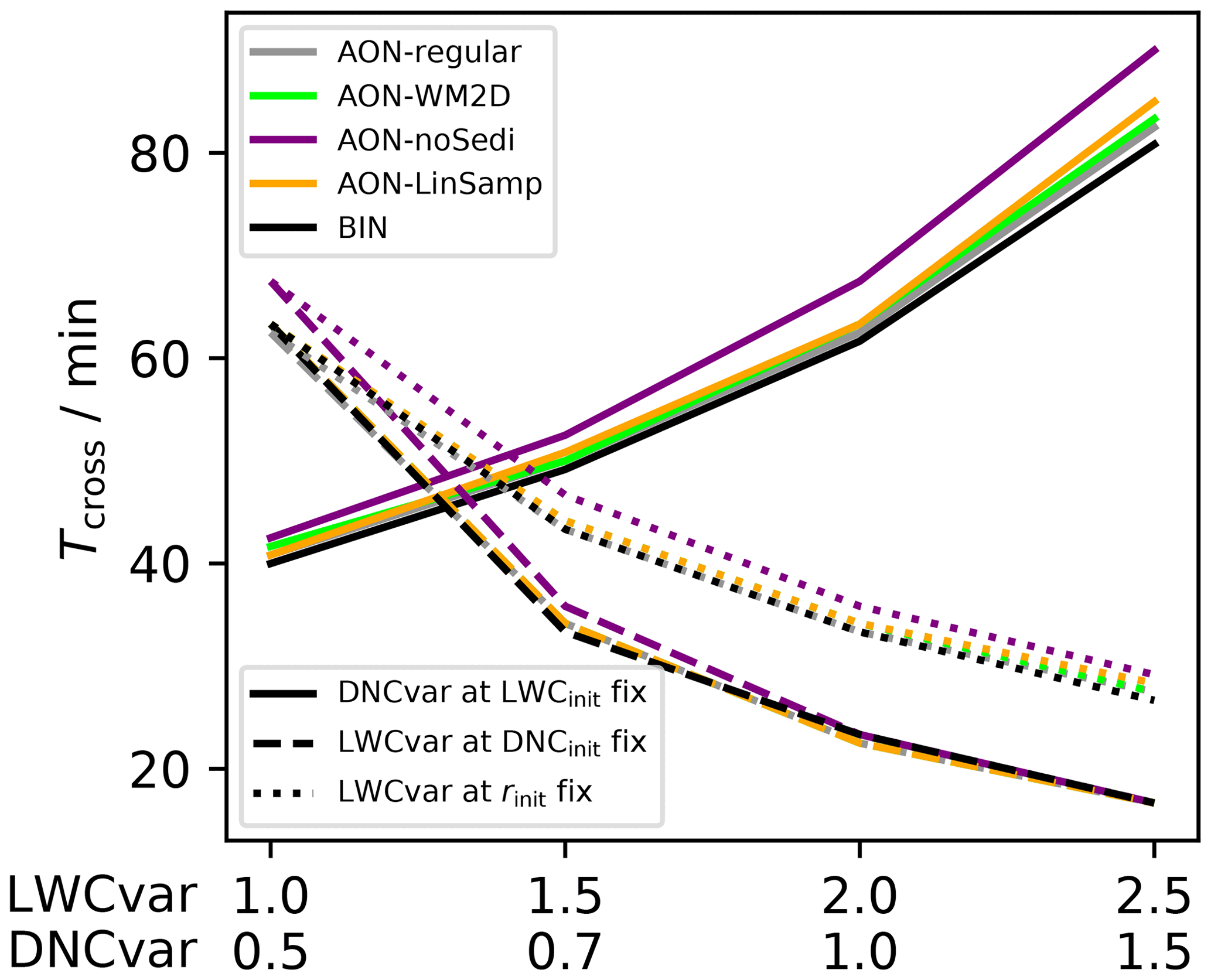
Figure 7BoxModelEmul set-up: sensitivities to the initial size distribution parameters LWCinit, rinit and DNCinit are summarised by showing Tcross, which is defined as the time when λ0 drops below 107 m−3. LWCinit is varied (the x axis shows the scaling factor LWCvar relative to the default LWCinit) for either fixed DNCinit (dashed lines) or rinit (dotted lines). The solid lines depict a DNCinit variation for fixed LWCinit. Again, the scaling factor DNCvar is depicted on the x axis. Five different model versions, as indicated in the top-left legend, are used: regular AON (reg), AON-WM2D, regular AON with noSedi (“nS”), AON with LinSamp (“LS”) and BIN.
In a first experiment, we increase LWCinit by a factor of 1.5 and repeat the κ sensitivity test; see Fig. 6e. We keep DNCinit fixed and hence the mean radius is µm. Compared to the base case with LWCinit=1 g m−3, λ0 starts to decrease after 20 min (instead of 40 min; see Fig. S10). Eventually, λ0 decreases below 104 cm−3 (instead of 106 cm−3). In the full simulations (all solid curves), we again find results nearly independent of κ for all tested AON versions (regular, LinSamp and WM2D). In the noSedi simulations (grey, dotted curve), fewer SIPs are necessary to obtain reasonable results compared to the base case in panel (a).
In a next step, the characteristics of the initial DSD are more systematically varied for fixed κ=40. For such a κ value the noSedi simulation of the base case was considerably off the reference. LWCinit=λ1(t0) is varied, for either fixed droplet number or fixed mean radius. The default value is scaled by a factor of 1.5,2.0 or 2.5. Similarly, DNCinit is varied by a factor of 0.5,0.7 or 1.5 keeping LWCinit constant.
A more detailed presentation of simulation results with time series of the mean diameter, λ0 and λ2 over 100 min is deferred to the Supplement (see Fig. S11). Here, we focus on a single metric again. We define Tcross as the time, when λ0 drops below 107 m−3. The smaller Tcross, the faster precipitation sets in. Figure 7 shows Tcross for all three sensitivity series (see lower left legend for the various line styles). Simulations with the BIN are contrasted with the regular AON, AON-WM2D, AON-noSedi and AON-LinSamp (see the top-left of the Fig. 7 for the various colours). Tcross and with it precipitation onset changes strongly with LWCinit and DNCinit. Generally, we find a similar behaviour across all tested models. The AON-noSedi version features the largest Tcross values. This is consistent with previous noSedi results in Fig. 5 where the decrease in λ0 lags behind. All other AON versions match well and are close to the BIN results. Only for the largest DNCinit value does some spread in Tcross exist. Figure S11 shows that BIN predicts in all cases slightly lower droplet numbers similar to what we already observed for the default microphysical initialisation in Fig. 5. Nevertheless, we can confirm the very good agreement of BIN and all full AON simulations.
As a last AON sensitivity study, the default Long kernel is replaced by the Hall kernel. Figure 6f shows the corresponding results. The decrease in λ0 occurs at a slower rate (the y scale now uses a linear scale). For the full simulations (solid curves), we obtain perfect agreement for any chosen κ value and for all three model versions. Moreover, convergence with κ in the noSedi simulations (dotted curve) is less critical than in the base case (compare with panel a again) and results converge for κ≥40. Time series of λ0 of all Hall kernel simulations are shown in Fig. S12.
So far, all reference BIN results were obtained with Wang's algorithm, using a time step Δt=1 s and resolution s=16. We conclude the box model emulation section by showing the sensitivities of two BIN versions. For this, we vary the bin resolution s and the time step for the base case with LWCinit=1 g m−3 and Long kernel and apply either Bott's or Wang's algorithm. The default time step is Δt=10 s as in the AON simulations and the bin resolution is s=4. Figure 6g–h show results obtained with Bott's and Wang's algorithm, respectively. Again, λ0 time series of these BIN simulations are shown in Fig. S13.
We find that Bott's algorithm converges for s≥2 (Fig. 6g). Wang's algorithm, on the other hand, does not produce stable results for higher resolutions and Δt=10 s. Thus, the time step had to be reduced (see inserted legend, for the combination of s and Δt). For s≥8 results have converged to the reference. Figure 6h shows the time step dependency for a medium resolution of s=4. While Bott yields stable results for Δt≤100 s, the results only converge for Δt≤20 s. We can even see a slight dependence of λ0(t=1 h) on Δt. As a side note, this is a clear indication that the BIN reference values used for orientation so far should not be interpreted as absolute reference, and it would be premature to discredit AON results being slightly above the BIN reference.
Wang's algorithm, on the other hand, requires Δt≤10 s for stable results, and convergence is reached for Δt≤5 s. Overall, we can conclude that both algorithms converge to basically the same values, given a sufficiently high s and small Δt is chosen. As Bott's algorithm appears to be more robust than Wang's algorithm, all following BIN simulations are carried out with this algorithm.
Comparing the various collisional growth algorithms, we find that Bott's algorithm has the least requirements in terms of bin resolution and time step as we have converged results for t up to 100 s and s as low as 2. AON simulations may converge for κ=5 (corresponds roughly to s=2) and Δt=10 s if GBs of the column are sufficiently interconnected and averaging over several realisations is done. Wang's algorithm produces correct solutions for s=4 and Δt=5 s, and yet increasing the bin resolution has to be done hand in hand with a reduction of the time step.
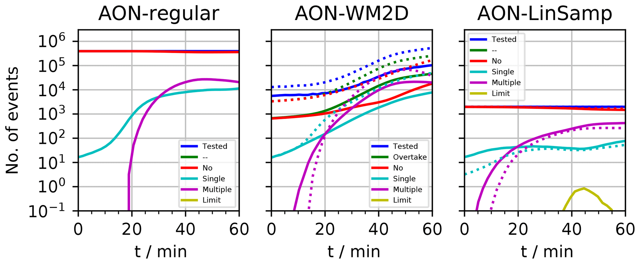
Figure 8BoxModelEmul set-up: time series of a number of events in the various AON versions. Shown are the number of tested SIP combinations, of overtakes, of no collection, of a single collection and of a multiple collection in every time step. Additionally, the number of limiter cases, where νcoll had to be artificially reduced, is shown (occurs only in the LinSamp panel). The parameter set-up is given in the text. In the WM2D panel, the dotted lines show the case with Δz=10 m. In the LinSamp panel, the dotted lines show the 1 s simulation. The displayed numbers can be below unity, as averages over 20 instances are shown.
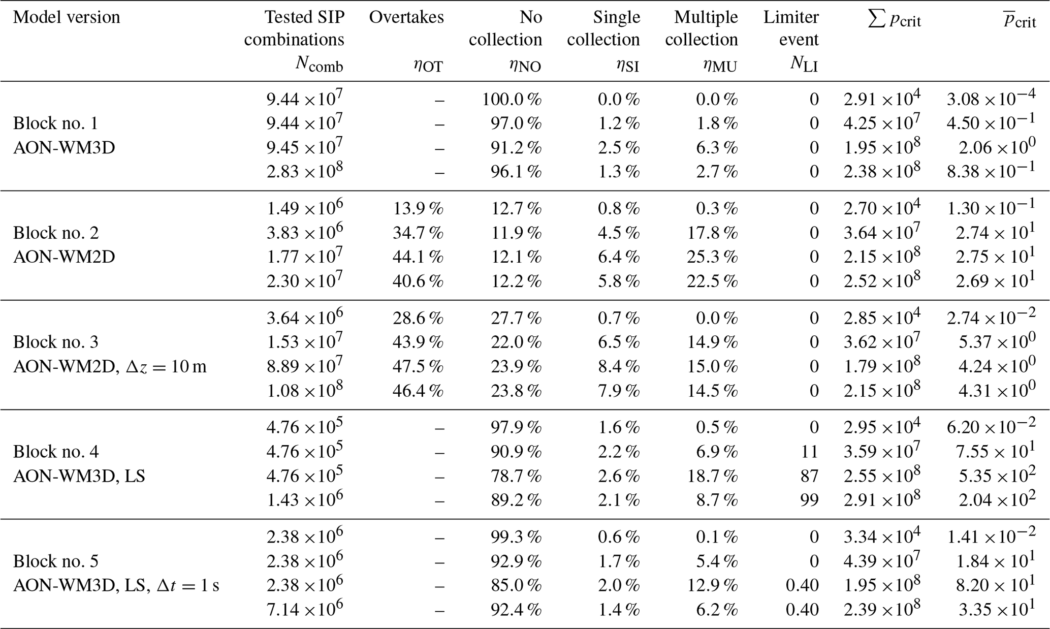
Table 3BoxModelEmul set-up: a number of events for various AON versions for the parameter set-up given in the text. Ncomb is the number of tested SIP combinations and NLI is the number of limiter cases, where νcoll had to be artificially reduced. Moreover, ηOT, ηNO, ηSI and ηMU specify the number of overtakes, no collections, single collections and multiple collections divided by Ncomb. The two last columns shows summed-up pcrit (summed over all times and SIP combinations and overtakes) and the average pcrit. For each AON simulation, the first three rows show aggregate values over three time periods (0–20, 20–40 and 40–60 min) and the fourth row values for the full time period.
3.2 Algorithm profiling
Now, we turn the attention to an algorithm profiling of the various AON versions.
Figure 8 and Table 3 give an example of how often collections occur in the model. For AON-WM2D, the number of overtakes is also given. The listed numbers give a rough indication of the importance of the various events (overtake, no collection, single collection, multiple collection, limiter), and yet we want to note the caveat that the relative importance changes with a change of the parameter set-up. Here, results are shown for the specific set-up with nz=20, nrinst=10, ΔV=1 m3, Δt=5 s, Δz=50 m and κ=40. The figure shows qualitatively the number of occurrences as a function of time, whereas the table gives aggregate values for three 20 min blocks and the total 60 min simulation period. In both WM3D versions (regular and LinSamp), the number of tested SIP combinations Ncomb is constant over time. Clearly, the LinSamp value is smaller by a factor of 200 (=NSIP) and implies a faster execution. For the WM2D version, on the other hand, Ncomb increases over time as the DSD gets more mature and larger droplets fall faster. Relative to the regular (WM3D) version, Ncomb of WM2D is at any time smaller. In the beginning of the simulation, possible overtakes occur among relatively few SIPs; much fewer on average than there are in a GB; hence the total Ncomb is around a factor of 60 smaller (in the first 20 min; 9.44×10⁷ vs. 1.49×10⁶). Even towards the end of the simulation, many SIPs are still small and travel through a small fraction of the GB. Only a few SIPs grow to raindrop size and travel distances of order Δz. The table shows that the total (time-integrated) Ncomb is more than a factor of 12 smaller for WM2D than for WM3D (2.30×10⁷ vs. 2.83×10⁸). This demonstrates the numerical efficiency of the current WM2D implementation despite a theoretically unfavourable computational complexity with a factor of nz higher Ncomb compared to the regular WM3D version.
Moreover, the workload per time step is constant in both WM3D versions and determined solely by NSIP. In the WM2D version, the workload depends additionally on the properties of the DSD and also on Δz. If Δz is reduced by a factor of 5 (see block no. 3 in the table), Ncomb roughly increases by the same factor. Similarly, we found a longer execution time of WM2D in the LWCup series than in the base case (not shown).
In the table, the ratios ηNO, ηSI and ηMU specify the number of no collections, single collections and multiple collections divided by Ncomb and add up to 100 % for both WM3D versions. In the regular WM3D version, only 1.3 % and 2.7 % of all tested combinations lead to a single or multiple collection. So, for most combinations pcrit is close to zero and makes a collection unlikely. On the other hand, for favourable SIP combinations pcrit can be far above 1 (imagine a SIP combination with νi=106, νj=102 and νcoll=104 yielding pcrit=100). This also explains the somewhat surprising fact that the average is close to unity (=0.83; see right-most column). The PDF (probability density function) of all pcrit values is strongly right-skewed (not shown). In the LinSamp case, single and multiple collections occur in 2.1 % and 8.7 % of the tested combinations. Collections are more likely as is larger due to the upscaling. Moreover, νcoll had to be artificially reduced in NLI≈100 cases. Note that such limiter cases do not appear in any QuadSamp version (regular and WM2D). In the LinSamp version, NLI can be cut down by choosing a smaller time step (see fifth block in table). Using Δt=1 s leads to 5 times smaller pcrit values, increases ηNO, and decreases ηSI and ηMU. Limiter cases are now an extremely rare event. For clarification, pcrit of a single SIP combination scales with Δt−1; from this, however, does not follow that the listed values of the two LinSamp simulation differ by a factor of 5, as the DSDs and SIP ensembles and weights evolve differently in the two simulations.
Finally, we focus on the WM2D version (block no. 2). Here, the sum of ηNO, ηSI and ηMU yields ηOT, the number of overtakes divided by Ncomb, and not 100 % as before. In the end, around 40 % of all tested SIP combinations undergo an overtake. This quite large fraction comes from the fact that the DSD (or more precisely the size distribution of the SIPs) features a strong bimodal spectrum. So most tested combinations are combinations between a large collector SIP i and a small SIP j with zi>zj. These tested SIP combinations fulfil by design . For small SIPs j, holds. As ϵ is a small distance, it is likely that is fulfilled; i.e. SIP i overtakes SIP j. In more than every second overtake, a multiple collection occurs (i.e. . In one-eighth (one third) of the overtakes a single collection (no collection) happens. So the relative importance of the various events is quite different compared to the regular AON and also is 3 times larger (2.69 vs. 0.83). Note that changing Δz in the WM2D simulation (block no. 3) also affects the relative occurrences of no collection, a single collection and multiple collections. In the WM3D versions, the overall workload is proportional to Δt−1. This is different in the WM2D version. With an increasing time step, droplets travel longer distances. Hence, the number of tested combinations and overtakes per time step increases.
Note that the relative occurrence frequency of pcrit values may depend also on the spectrum of given νp values (i.e. on the SIP initialisation method), which is not elaborated here.
Figure S14 demonstrates that all five AON simulations converge and show a basically identical time evolution of λ0. The analysis here shows that in the end more multiple collections than single collections appeared. Clearly, the occurrence of multiple collections in a simulation does not necessarily deteriorate the simulation results. It is certainly not the case that the time step choice or adaptation must be such that multiple collections barely appear in a simulation. Beyond that, limiter events that occurred in the LinSamp simulation with Δt=10 s did not avert convergence. So even a certain amount of limiter events seems to be acceptable in terms of performance. Figure 6b showed that even for Δt=100 s LinSamp and regular AON produce similarly good results, albeit off from the reference.
Several of the above findings may hold only for the specific set-up used here. To put the findings into a broader context, we next derive scaling relations for basic numerical quantities and, in particular, discuss their sensitivity to the time step and the number of SIPs. For a simplified presentation, we limit ourselves to the regular and LinSamp version and assumed converged simulation results and no limiter events. Moreover, we assume that an increase in NSIP leads to a uniform decrease in all SIP weights νp.
For the following basic quantities we have
where γcorr is the correction factor defined in Eq. (25). For QuadSamp α=2, β=0 and for LinSamp α=1, β=1.
Accordingly,
In both versions, νsum is independent of NSIP and δt. Clearly, νsum should have the same value (not only the same asymptotic behaviour) across all AON versions in order to obtain consistent results. The average probability scales, not surprisingly, linearly with δt. For QuadSamp, is inversely proportional to NSIP and an increase in NSIP decreases the occurrence of multiple collections and limiter events. In the LinSamp case, is independent of NSIP (as already pointed out by Shima et al., 2009, end of their Sect. 5.1.3) implying that an increase in NSIP does not decrease the number of multiple collections and limiter events. Nevertheless, an NSIP increase is also beneficial in LinSamp as it increases the number of trials and reduces the variance of the results.
3.3 Realistic column model simulations
The box model emulation simulations presented in Sect. 3.1 used an academic and unrealistic set-up, not yet exploiting the capabilities of a column model framework. The following two subsections treat realistic set-ups.
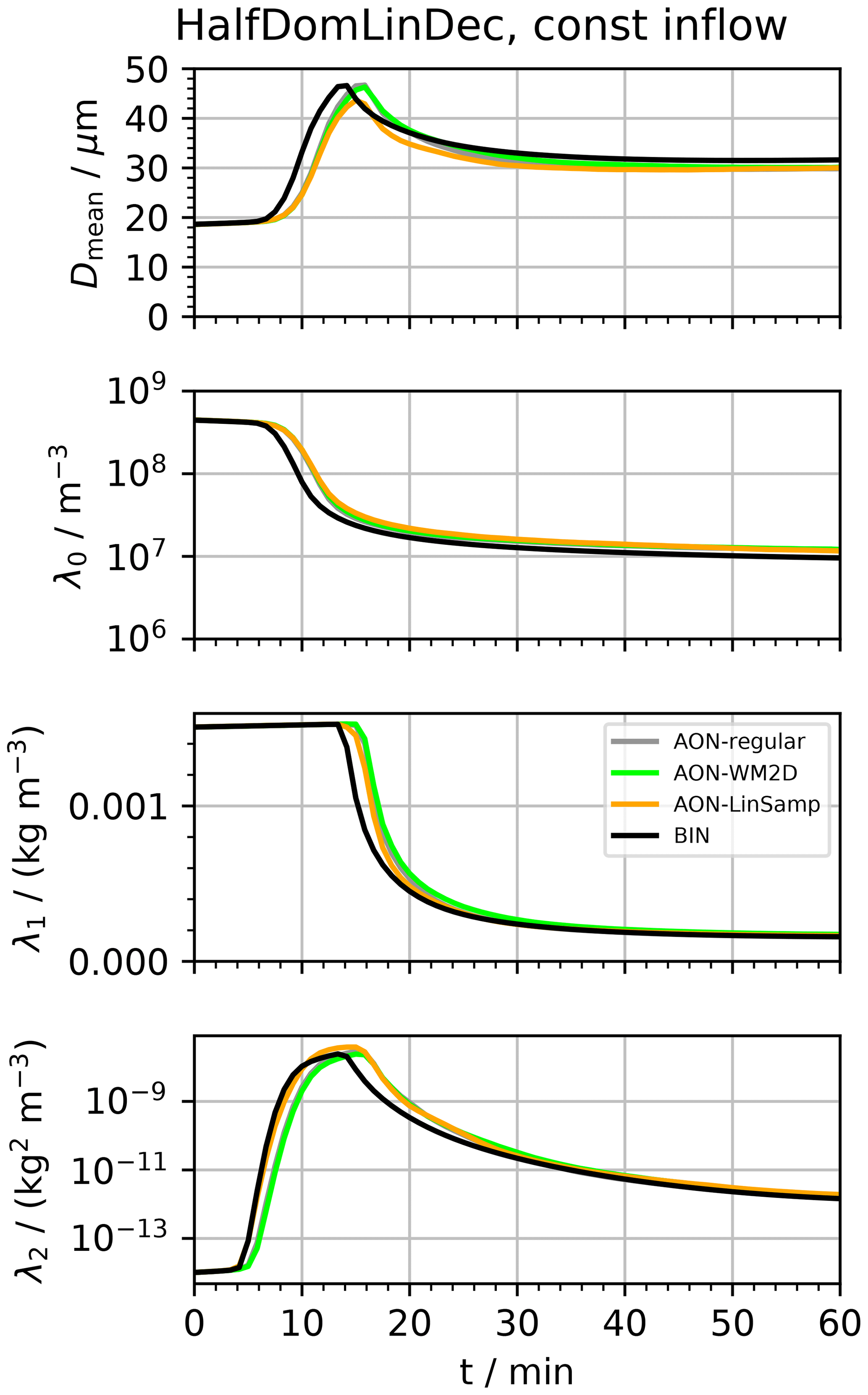
Figure 9HalfDomLinDec set-up: temporal evolution of Dmean and column-averaged moments λ0,λ1 and λ2 for various model versions (see inserted legend; “LS” is short for linear sampling).
3.3.1 Half domain set-up
We initialise droplets in the upper half of a 4 km column. In each GB the mean radius of the DSD is fixed at the default value rinit=9.3 µm. LWCinit (and with it DNCinit) decreases linearly from 3 g m−3 at the model top to zero at z=2 km. At the model top, a constant influx of a DSD with LWCinit=3 g m−3 is prescribed, which guarantees a smooth profile over time. Otherwise, a discontinuity would occur at the top-most GB which may cause problems in the BIN model. The further settings are nz=400, Δz=10 m, Δt=10 s, nrinst=20, κ=40. All figures related to this set-up start their caption with the label “HalfDomLinDec set-up”.
Figure 9 shows the temporal evolution of the mean diameter and the moments λ0, λ1 and λ2. Due to the influx condition, the total mass increases during the first 10 min, barely visible in the third panel. During this period, however, collisional growth is already efficiently reducing the droplet number. This is accompanied by an increase in the mean diameter and radar reflectivity. Soon after, the first droplets reach the surface, the mass declines rapidly, and the whole column is more or less washed out after 30 min. We find an excellent agreement among the four model versions BIN, AON-regular, AON-WM2D and AON-LinSamp.
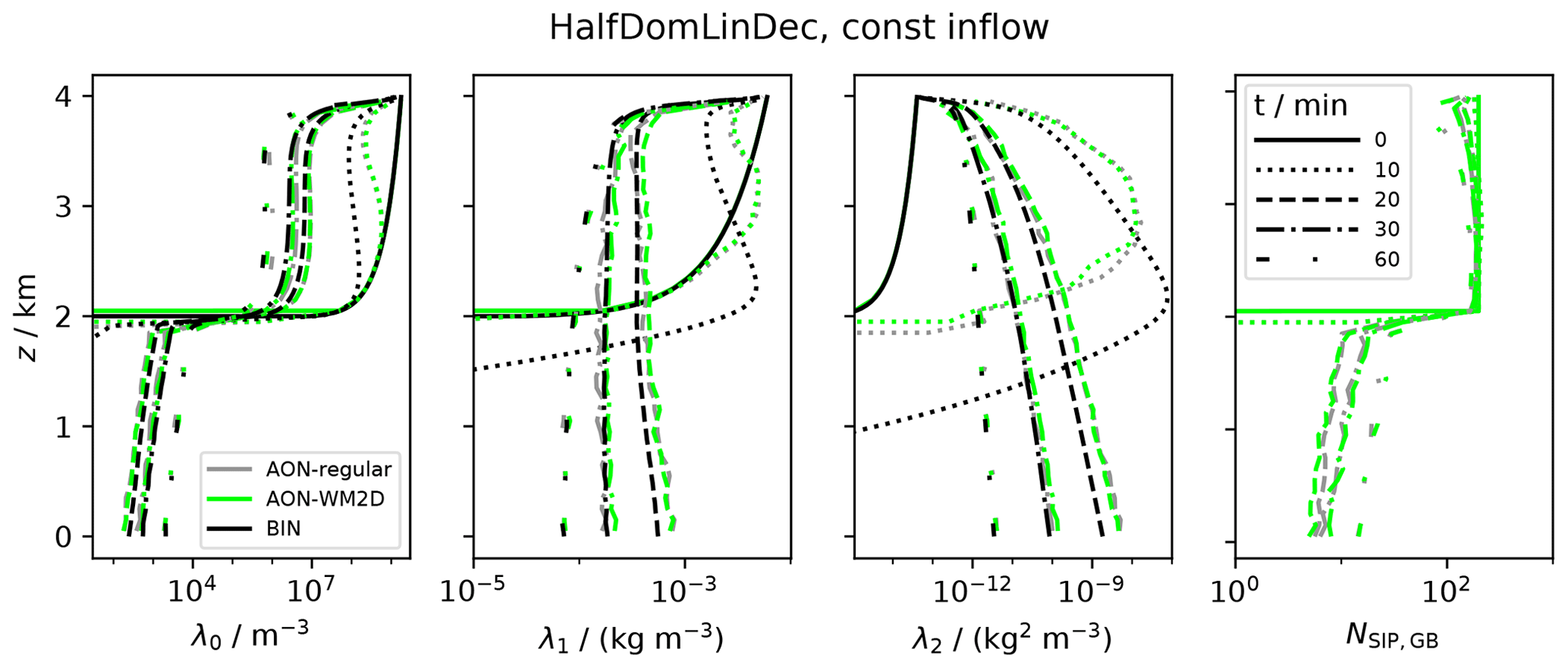
Figure 10HalfDomLinDec set-up: vertical profiles of moments λ0, λ1, λ2 and NSIP,GB for various model versions (AON-WM3D, AON-WM2D, BIN; see colour legend in left-most panel) and times (0, 10, 20, 30, 60 min; see line style legend in right-most panel).
Figure 10 shows vertical profiles of DNC, LWC, Z and NSIP,GB for times t=0, 10, 20, 30 and 60 min. In the upper half, droplet number is roughly homogeneously distributed and decreases over time. In the lower half, droplet number concentrations are several orders of magnitude smaller than in the upper half and increase over time. The profile of the radar reflectivity shows the highest values after 10 min with a pronounced peak in the middle of the domain. Soon after, the Z profiles become smooth and increase monotonically towards the surface. The sedimentation flux also increases towards the surface, and hence λ2 values decrease over time.
In the upper half, NSIP,GB is fairly constant over altitude and time with around 200 SIPs. As the LWC is initially highest at the model top, collisional growth is most frequent there. Most likely, SIPs from that layer turn into collector SIPs, meaning they fall through the total column and collect many other SIPs. Consistently, NSIP,GB decreases over time close to the model top. Yet overall, only a small fraction of the SIPs becomes raindrops eventually (see for example Fig. 4 in U2017) and hence the SIP number is substantially smaller in the lower half. There, each GB is populated by roughly 10 SIPs. Despite this rather small value, convergence in DNC and Z seems to be ubiquitous.
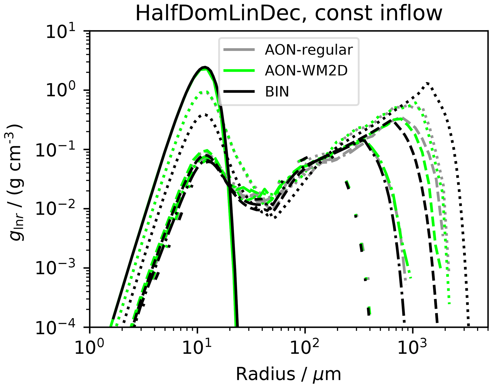
Figure 11HalfDomLinDec set-up: size distribution gln r for various model versions and times as in Fig. 10 (see legends there).
Figure 11 depicts column-averaged DSDs for various points in time. The precipitation mode develops rapidly, and 2 to 3 mm sized drops are produced within 10 min. Those drops soon reach the surface and remove a significant amount of liquid water from the column. Due to this wash-out effect, the raindrops cannot grow that large any longer and the precipitation mode peaks at smaller sizes at later times.
For a cleaner presentation, AON-LinSamp results were not shown in Figs. 10 and 11, but we confirm that these are very similar to those from AON-regular and AON-WM2D.
Overall, the agreement between the four model versions is remarkable given the completely different numerics of the Eulerian and Lagrangian approach.
Next, the vertical resolution Δz is varied in the model versions AON-regular, AON-WM2D and BIN (see Fig. S17). Even though this may look like a trivial sensitivity study, the effect of a Δz variation has different implications in the various models and AON versions. The differences are rather subtle. First, Δz affects the number of GBs nz and with it the total SIP number NSIP,tot (as NSIP,GB is unchanged with the standard SIP-init technique). To eliminate this unwanted numerical side effect in LCM1D, we increase NSIP,GB proportionally to Δz (analogous to the ΔV sensitivity tests in Sect. 3.1). Second, the advection by sedimentation changes in BIN as the CFL number changes and the subcycling has to be adapted. In LCM1D, the SIP transport by sedimentation is independent of the assumed grid and clearly unaffected by a Δz variation. Third, there is a physical effect as Δz determines the layer depth of the well-mixed volume (effective only in AON-regular and BIN).
It follows that the results of the AON-WM2D version should be independent of Δz. Moreover, the AON-regular version can be used to determine if the size (more specifically the depth) of the well-mixed volume is a crucial parameter. In bin models in general, this sensitivity could not easily be singled out as sedimentation numerics also change with Δz.
Given a constant column height Lz=4 km, Δz takes the values 2, 10, 50 or 100 m and we find λ0(t) to be independent of Δz (see Fig. S17). As expected, the AON-WM2D simulations are not at all affected by Δz. In particular, the AON-regular simulations are insensitive to a change in Δz and imply that the depth of the well-mixed volume has a negligible impact on the extent of collections in the present set-up. Interestingly, the Δz=10 m simulation uses NSIP,GB=200 and the Δz=100 m simulation NSIP,GB=2000. Hence, a factor of 100 more SIP combinations are tested for possible collections in the latter case, yet with no effect on the physical evolution.
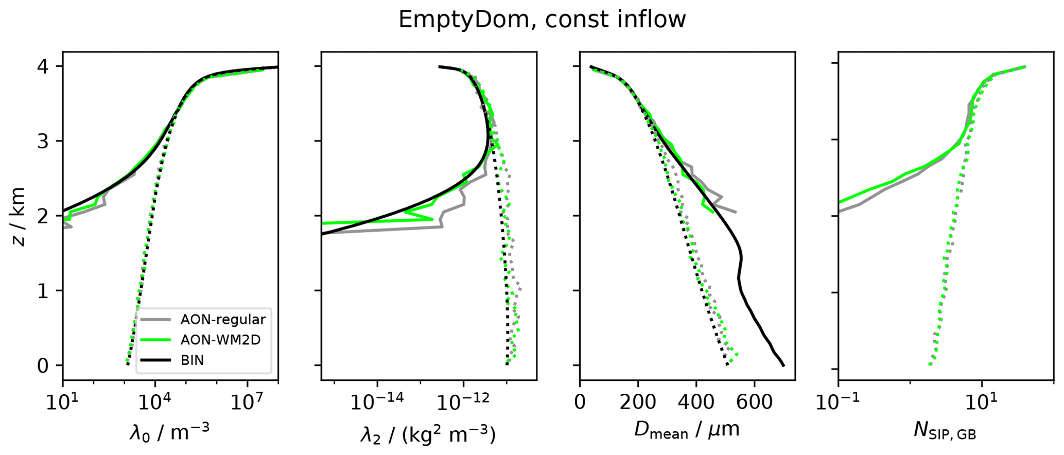
Figure 12EmptyDom set-up: vertical profiles of moments λ0, λ2, Dmean and NSIP,GB for various model versions (see legend). Depicted are the times t=30 and 60 min (solid, dotted).
3.3.2 Empty domain set-up
In this section, the 4 km deep column is initially devoid of droplets and a time-constant influx of a DSD with rinit=16.9 µm and LWCinit=6 g m−3 is prescribed. As in the box model emulation set-up, the corresponding DNCinit is 297 cm−3. All figures related to this set-up start their caption with the label “EmptyDom set-up”.
Over time the column fills with droplets, a distinct size sorting is established and DSDs at a specific altitude are expected to be rather narrow. Hence, choosing a vertical resolution that is too coarse may result in overestimating collections as the droplets are not supposed to be well-mixed within such deep GBs. In such a case, the AON-WM2D version has a conceptional advantage as it does not assume well-mixedness in the vertical direction. The chosen set-up specifically aims to demonstrate the possible improvement by this. Again, the further parameter settings are nz=400, Δz=10 m, Δt=10 s, nrinst=20, κ=40.
Figure 12 shows vertical profiles at t=30 and 60 min for AON-regular, AON-WM2D and BIN. After 30 min the cloud roughly covers the top half of the column. Below z=2 km, fewer than 0.1 SIPs are present in each GB of LCM1D. This implies that only in 1 or 2 out of the 20 realisations do SIPs grow sufficiently large to fall that far. This also explains the jagged λ2 profiles in the lower part. Below a certain altitude, no SIPs are present at all and hence no mean droplet diameter could be diagnosed. BIN produces non-zero mass and number all the way down to the bottom and allows a smooth Dmean profile to be computed. As the predicted droplet masses and concentrations become vanishingly small, the derived Dmean values in the lower part are, however, meaningless. Anyhow, this small discrepancy between BIN and LCM1D is a transient phenomenon. Once the cloud is fully developed, the profiles match perfectly (see dotted curve for t=60 min). The fact that on average well below 10 SIPs populate GBs in the lower domain half is remarkable. Nevertheless, the LCM1D results seem to be converged. SIPs at those altitudes are large (Dmean>400 µm) and fall fast, which fosters a strong SIP exchange across GBs and is beneficial to convergence (see Sect. 3.1). The AON-LinSamp simulation (not shown) produces again very similar profiles. This is even more remarkable, as on average only 5 SIP pairs are tested for collections per GB in the lower half.

Figure 13EmptyDom set-up: temporal evolution of Dmean and column-averaged moments λ0 and λ2 for various model versions (see legend).
Figure 13 shows the temporal evolution of the mean diameter, column-averaged DNC and Z; here AON-LinSamp curves are added. Within the first 10 min, DNC increases quickly. Soon after, collection becomes effective and DNC reaches a quasi-steady state. The radar reflectivity increases within the first 60 min and then also reaches a quasi-steady state. The only discrepancies between the various models are slightly larger DNC values by all AON versions. The reason for this is elucidated next.

Figure 14EmptyDom set-up: temporal evolution of column-averaged moments λ0 and λ2 for various model versions (AON-WM2D, a; AON-WM3D, b; BIN, c). Each panel shows a variation of the vertical resolution Δz (see legend in the left panel). In LCM simulations, SIP numbers for Δz=100 and 50 m simulations are increased to the level of the Δz=10 m simulation.
Fig. 14 shows the Δz dependence of the DNC evolution in the different models. For Δz=50 and 100 m, the SIP numbers in AON simulations have been upscaled to maintain NSIP,tot values comparable to the Δz=10 m simulation (as already done in the HalfDom set-up). The Z evolution (see Fig. S19 for a time series) is found to be basically independent of Δz in all three models. For the DNC evolution, we find also no Δz dependence in the WM2D model as intended. However, in AON-regular and BIN models, DNC levels off at different values depending on Δz. This behaviour is most likely caused by an interaction of the unresolved size sorting and the hence larger range of potential collection partners in AON-regular and BIN. Apparently, this results in changes in the rate with which the smallest droplets are collected by larger droplets, as indicated by the substantial effect of this process on DNC, but not on Z.
The Δz dependence persists in AON-LinSamp simulations and in further AON-regular simulations, where we reduced the time step to Δt=1 s or decreased NSIP,tot (see Fig. S20).
This undesired Δz dependence in BIN and AON-regular seems to showcase the superiority of the AON-WM2D version. However, the Δz dependence does not affect higher moments of the DSD, e.g. Z (as shown in the Supplement) or the accumulated size distribution of all droplets that crossed the lower boundary (Fig. S21). Accordingly, precipitation-related quantities seem to be unaffected by changes in the vertical grid spacing. On the other hand, most of the Δz effect can be attributed to changes in the DNC within the top-most 100–200 m of the column (Fig. 12). Anyhow, based on the presented results, we cannot definitely answer the question of whether using the AON-WM2D approach has in general any practical benefits over the classical 3D well-mixed approaches. Further research in this direction is required.
Collection, i.e. the coalescence, accretion and aggregation of hydrometeors, is an important process for the development of precipitation in liquid-, mixed- and ice-phase clouds, respectively. The correct representation of these processes in cloud microphysical models is, therefore, of utmost importance. In this study, we investigated and validated the representation of collection in LCMs, a relatively new approach that uses simulation particles, so-called SIPs or super-droplets, to represent cloud microphysics.
This study is a continuation of U2017, in which we analysed various representations of collisional growth algorithms in LCMs using zero-dimensional box model simulations. Here, this analysis is extended to one-dimensional column simulations that allow the effects of sedimentation to be explicitly considered. This study focuses on the AON algorithm (Shima et al., 2009; Sölch and Kärcher, 2010) that outperformed other collection algorithms, as assessed in our previous study (U2017). Two versions of AON are applied that differ in the assumed distribution of droplets represented by a SIP: in the regular AON version, the droplets are assumed to be well-mixed within a three-dimensional volume (which is typically identical to the GB of the dynamical model coupled to the LCM). In WM2D, the height coordinate of each SIP is used explicitly, and the droplets represented by a SIP are assumed to be well-mixed only within a two-dimensional, horizontal plane. Accordingly, collections are only considered if a SIP overtakes another one during a time step.
Furthermore, two variants of AON-WM3D are tested that differ in the number of SIP combinations that need to be tested during collection. In its simplest form, AON-WM3D depends quadratically on the number of SIPs since every SIP may interact with any other SIP inside a GB (QuadSamp). Additionally, Shima et al. (2009) introduced an approach that depends only linearly on the number of SIPs by appropriately scaling collection probabilities (LinSamp). What we call here AON-LinSamp is also referred to as the SDM (super-droplet method) algorithm in the literature.
All results are compared to established Eulerian bin model results (Bott, 1998; Wang et al., 2007). Accordingly, the capability of Lagrangian and Eulerian approaches to advect a droplet ensemble due to sedimentation is tested first – neglecting the influence of collection. Since numerical diffusion is inherent to any Eulerian advection problem, i.e. also sedimentation, its impact might impede any conclusions drawn from the collection simulations. However, by using an appropriate advection scheme (MPDATA, Smolarkiewicz, 1984), numerical diffusion can be reduced to an acceptable degree in the sense that the present simulations focus on the differences driven by collection numerics.
As a first step and link to U2017 simulations, box model simulations are emulated in the column model. This is done by initialising each GB of the column with the same droplet size distribution and applying cyclic boundary conditions at the surface and the top. By using this framework, we were able to show that sedimentation increases the model convergence rate significantly compared to box model simulations without sedimentation; i.e. fewer SIPs per GB are required in the column model. The reason for this behaviour is that the largest and hence fastest-falling droplets are no longer confined to the same GB and to the same potential collection partners, which increases the ensemble of potential collection partners. A similar observation has been made by Schwenkel et al. (2018), who used randomised motions between individual GBs. Overall, these results indicate that a simulation with only 24 SIPs per GB can yield reasonable results if (i) these SIPs are able to move between GBs and (ii) the SIP weighting factors are ideally chosen in the beginning by using an appropriate SIP initialisation technique.
In general, a remarkably good agreement of the LCM results with the bin reference has been found for all AON versions (regular AON, AON-WM2D and AON-LinSamp). AON-LinSamp results are only slightly worse compared to regular AON simulation of the same time step and SIP number. However, these stronger restrictions on the time step do not at all outweigh the computational benefit gained by the favourable linear computational complexity, making the LinSamp version the preferred choice if computation time is a critical factor. In an operational setting, the QuadSamp approach is a valuable alternative to LinSamp as long as the number of SIPs is not prohibitively high.
We further compared the computational requirements for the WM2D and WM3D implementations of AON. We found that WM2D requires checking for overtakes in the entire column, not only in the GB in which the SIP is located, as is the case for WM3D. However, this seeming disadvantage is turned into an advantage, since only a minority of SIPs overtakes other SIPs. Accordingly, the overall number of calculations necessary for the application of WM2D is reduced compared to WM3D. The physical reason for this effect is the typical bimodal structure of droplet spectra, which consist of only a few large droplets that sediment and collect other droplets efficiently, while the remaining droplets are usually too small to sediment and collect other droplets.
Finally, we applied the various AON versions to two more realistic column cases. While both cases use a prescribed inflow of droplets from the top, the first case is initialised with a linearly increasing liquid water content, and the second case is completely devoid of any initial droplets. Overall, the agreement of AON-regular, AON-WM2D, AON-LinSamp and the bin references is remarkable. Only in the second case, which is designed to be heavily prone to size-sorting, is a dependence on the vertical grid spacing detectable for WM3D and the bin reference, which both assume droplets to be well-mixed within a GB, while the WM2D results are found to be completely independent of the vertical grid spacing.
In all AON variants, simulation results converge for fairly large time steps Δt>10 s. For such high Δt values, the largest droplets routinely travel distances larger than the vertical resolution Δz during one time step (as noted above). Whereas in Eulerian advection this would violate the CFL criterion and cause a numerical break-down, Lagrangian numerics do not fail. In higher-dimensional full microphysical models with diffusional growth included and gradients in moist thermodynamic fields, physical reasons also render it appropriate to apply a time step criterion in the spirit of the CFL condition in Lagrangian approaches. Solving diffusional growth usually sets stricter bounds on Δt (Arnason and Brown, 1971). Moreover, the interplay of diffusional and collisional growth, which was not studied here, may raise the time step requirements of AON for physical reasons. For example Dziekan et al. (2019), using AON with linear sampling in 2D and 3D LCM simulations, found convergence only for a rather small time step of Δt=0.1 s.
All in all, this study has shown that the representation of collisional growth in LCMs using AON successfully reproduces established Eulerian bin results. This ability, of course, depends foremost on the number of SIPs and the applied time step as already indicated in previous zero-dimensional box model studies. Compared to these zero-dimensional studies, the application of an LCM in a column decreases the required number of SIPs significantly. The consequently lower computational costs raise hopes to use LCMs more frequently in large-scale, multidimensional models in the future.
This Appendix presents pure sedimentation test cases that are suited to demonstrating that minor differences are introduced by the different numerical treatment of the sedimentation process. Two simple set-ups with an influx of an exponential DSD with rinit=50 µm are tested. In the first case, the domain is initially empty and fills over time (EmptyDom) as in Sect. 3.3.2. In the second case, the upper half of the domain is filled, with LWCinit and DNCinit decreasing linearly to zero from the domain top to the domain middle (HalfDom) like in Sect. 3.3.1. Figure A1 shows the vertical profiles of normalised zeroth (a and c) and second (b and d) moments for EmptyDom (a and b) and HalfDom (c and d). Because of the lack of numerical diffusion, the solid LCM curves show the exact results, except for the error introduced by discretising the influx DSD with a probabilistic approach. Each panel showcases a convincing agreement between the Eulerian and Lagrangian approach. Only the BIN-US1 solutions are slightly smeared out. The small wiggles in the LCM curves originate from the probabilistic influx condition. Even though the above agreement is favourable, it might be that the advection errors of differently sized droplets compensate each other in the Eulerian approaches. Hence, in a second validation step, the computation of mass profiles is confined to certain droplet size ranges. Figure A2 shows such vertical profiles for EmptyDom. We see that for all four size ranges, the BIN results are smeared out relative to LCM. For the smallest size ranges both BIN versions are equally “bad” (panel a). For the three remaining panels, the MPDATA curves (dashed) are closer to the LCM reference than the US1 curves (dotted). On the other hand, the MPDATA curves in panel (d) show some wiggles. Overall, the agreement between LCM and BIN-MPDATA is good. The discrepancies introduced by the different sedimentation treatment appear to be small enough to warrant a focus on the collisional growth process and its implementations in the main part of the paper.
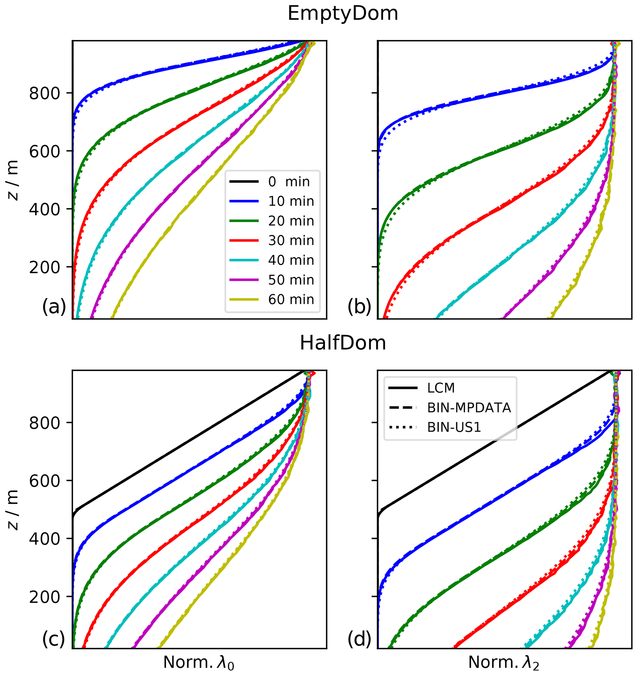
Figure A1Pure sedimentation test case: comparison of BIN and LCM (solid) advection. BIN uses either MPDATA (dashed) or first-order upstream scheme (dotted). EmptyDom (a, b) and HalfDom (c, d) set-ups are used with an exponential distribution with rinit=50 µm as influx condition. Displayed are vertical profiles of normalised zeroth and second moment at the indicated points in time.
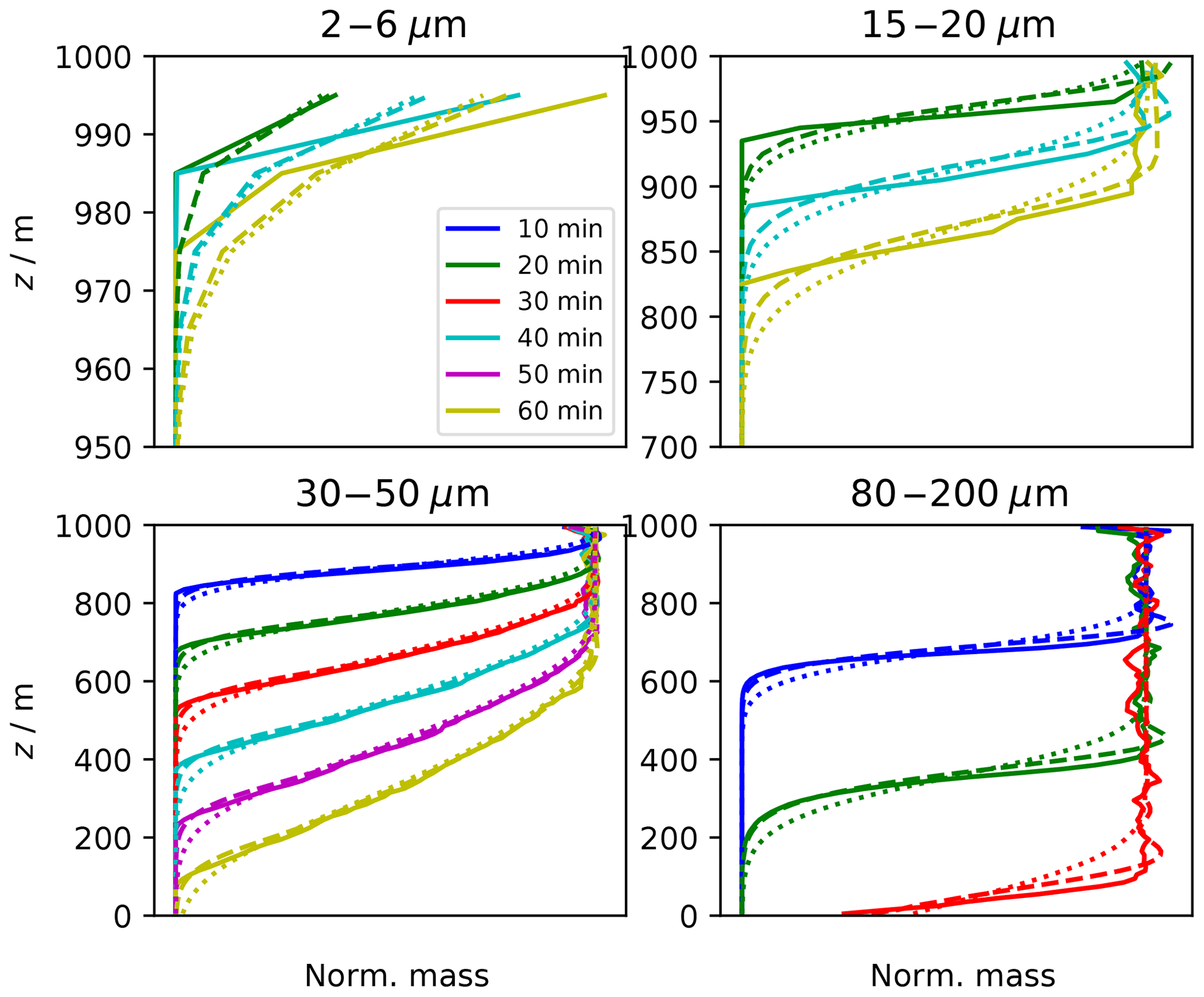
Figure A2Pure sedimentation test case: comparison of BIN and LCM advection. EmptyDom set-up with an exponential distribution with rinit=50 µm as influx condition. Displayed are vertical profiles of normalised mass within specified size ranges (see the heading of each panel) at the indicated points in time. Note that most panels use different y-axis ranges and do not show all six points in time.
Moreover, we tested the sensitivity to rCFL and Δt as both parameters in combination determine the local CFL number of each grid box. BIN simulations were carried out for the HalfDomLinDec set-up and with switched-on collisional growth (i.e. the set-up of Sect. 3.3.1). Figure S18 demonstrates that this has no impact on the prediction of the total moments.
The source code of the Lagrangian column model is hosted on GitHub (https://github.com/SimonUnterstrasser/ColumnModel, last access: 22 October 2020) and released under Apache License 2.0. The (frozen) code version used to produce the simulation data of this study can be obtained from Zenodo (https://doi.org/10.5281/zenodo.4031214, Unterstrasser, 2020a). The data of the BIN and AON simulations, together with all plot scripts that are necessary to reproduce the figures of this study, are in a second Zenodo data set (https://doi.org/10.5281/zenodo.4030878, Unterstrasser, 2020b). The source code of the bin collection algorithms by Bott (1998) and Wang et al. (2007) have been obtained from Andreas Bott and Lian-Ping Wang, respectively. We are not in the position to make the codes publicly available.
The supplement related to this article is available online at: https://doi.org/10.5194/gmd-13-5119-2020-supplement.
SU designed the study, programmed the Lagrangian column model, carried out the simulations and wrote most parts of the paper. FH discussed the results with the first author and wrote the introduction and conclusions. A first code version and preliminary results were obtained during the master's thesis of ML.
The authors declare that they have no conflict of interest.
We thank Lian-Ping Wang and Andreas Bott for providing box model versions of their collection algorithms. The first author thanks Jan Bohrer (Tropos Leipzig) for carefully examining the AON code and spotting the bug mentioned in Sect. 3.1.1. Moreover, we appreciate comments on the paper by Klaus Gierens. We thank the reviewers Shin-ichiro Shima, Sylwester Arabas and one anonymous reviewer for helpful comments which helped to improve the paper. This research was performed while Fabian Hoffmann held a Visiting Fellowship of the Cooperative Institute for Research in Environmental Sciences (CIRES) at the University of Colorado Boulder and the NOAA Earth System Research Laboratory.
The article processing charges for this
open-access publication were covered by a Research
Centre of the Helmholtz Association.
This paper was edited by Samuel Remy and reviewed by Sylwester Arabas, Shin-ichiro Shima, and one anonymous referee.
Alfonso, L. and Raga, G. B.: The impact of fluctuations and correlations in droplet growth by collision–coalescence revisited – Part 1: Numerical calculation of post-gel droplet size distribution, Atmos. Chem. Phys., 17, 6895–6905, https://doi.org/10.5194/acp-17-6895-2017, 2017. a, b
Alfonso, L., Raga, G. B., and Baumgardner, D.: The validity of the kinetic collection equation revisited, Atmos. Chem. Phys., 8, 969–982, https://doi.org/10.5194/acp-8-969-2008, 2008. a
Andrejczuk, M., Reisner, J. M., Henson, B., Dubey, M. K., and Jeffery, C. A.: The potential impacts of pollution on a nondrizzling stratus deck: Does aerosol number matter more than type?, J. Geophys. Res., 113, D19204, https://doi.org/10.1029/2007JD009445, 2008. a
Andrejczuk, M., Grabowski, W. W., Reisner, J., and Gadian, A.: Cloud-aerosol interactions for boundary layer stratocumulus in the Lagrangian cloud model, J. Geophys. Res., 115, D22214, https://doi.org/10.1029/2010JD014248, 2010. a
Arabas, S., Jaruga, A., Pawlowska, H., and Grabowski, W. W.: libcloudph++ 1.0: a single-moment bulk, double-moment bulk, and particle-based warm-rain microphysics library in C++, Geosci. Model Dev., 8, 1677–1707, https://doi.org/10.5194/gmd-8-1677-2015, 2015. a, b
Arnason, G. and Brown, Philip S., J.: Growth of Cloud Droplets by Condensation: A Problem in Computational Stability, J. Atmos. Sci., 28, 72–77, https://doi.org/10.1175/1520-0469(1971)028<0072:GOCDBC>2.0.CO;2, 1971. a
Bayewitz, M. H., Yerushalmi, J., Katz, S., and Shinnar, R.: The Extent of Correlations in a Stochastic Coalescence Process, J. Atmos. Sci., 31, 1604–1614, https://doi.org/10.1175/1520-0469(1974)031<1604:TEOCIA>2.0.CO;2, 1974. a, b, c, d
Beard, K. V.: Terminal Velocity and Shape of Cloud and Precipitation Drops Aloft, J. Atmos. Sci., 33, 851–864, https://doi.org/10.1175/1520-0469(1976)033<0851:TVASOC>2.0.CO;2, 1976. a
Beard, K. V. and Ochs III, H. T.: Collection and coalescence efficiencies for accretion., J. Geophys. Res., 89, 7165–7169, https://doi.org/10.1029/JD089iD05p07165, 1984. a
Berry, E. X.: Cloud Droplet Growth by Collection, J. Atmos. Sci., 24, 688–701, https://doi.org/10.1175/1520-0469(1967)024<0688:CDGBC>2.0.CO;2, 1967. a, b, c
Berry, E. X. and Reinhardt, R. L.: An Analysis of Cloud Drop Growth by Collection: Part I. Double Distributions, J. Atmos. Sci., 31, 1814–1824, https://doi.org/10.1175/1520-0469(1974)031<1814:AAOCDG>2.0.CO;2, 1974. a
Bott, A.: A Flux Method for the Numerical Solution of the Stochastic Collection Equation, J. Atmos. Sci., 55, 2284–2293, https://doi.org/10.1175/1520-0469(1998)055<2284:AFMFTN>2.0.CO;2, 1998. a, b, c, d, e
Bott, A.: A Flux Method for the Numerical Solution of the Stochastic Collection Equation: Extension to Two-Dimensional Particle Distributions, J. Atmos. Sci., 57, 284–294, https://doi.org/10.1175/1520-0469(2000)057<0284:AFMFTN>2.0.CO;2, 2000. a
Boucher, O., Randall, D., Artaxo, P., Bretherton, C., Feingold, G., Forster, P., Kerminen, V.-M., Kondo, Y., Liao, H., Lohmann, U., Rasch, P., Satheesh, S. K., Sherwood, S., Stevens, B., and Zhang, X. Y.: Clouds and aerosols, in: Climate change 2013: the physical science basis. Contribution of Working Group I to the Fifth Assessment Report of the Intergovernmental Panel on Climate Change, Cambridge University Press, 571–657, 2013. a
Dziekan, P. and Pawlowska, H.: Stochastic coalescence in Lagrangian cloud microphysics, Atmos. Chem. Phys., 17, 13509–13520, https://doi.org/10.5194/acp-17-13509-2017, 2017. a, b, c, d, e
Dziekan, P., Waruszewski, M., and Pawlowska, H.: University of Warsaw Lagrangian Cloud Model (UWLCM) 1.0: a modern large-eddy simulation tool for warm cloud modeling with Lagrangian microphysics, Geosci. Model Dev., 12, 2587–2606, https://doi.org/10.5194/gmd-12-2587-2019, 2019. a, b
Gillespie, D. T.: The Stochastic Coalescence Model for Cloud Droplet Growth, J. Atmos. Sci., 29, 1496–1510, https://doi.org/10.1175/1520-0469(1972)029<1496:TSCMFC>2.0.CO;2, 1972. a, b, c
Grabowski, W. W., Morrison, H., Shima, S.-i., Abade, G. C., Dziekan, P., and Pawlowska, H.: Modeling of Cloud Microphysics: Can We Do Better?, B. Am. Meteorol. Soc., 100, 655–672, https://doi.org/10.1175/BAMS-D-18-0005.1, 2019. a
Hall, W. D.: A Detailed Microphysical Model Within a Two-Dimensional Dynamic Framework: Model Description and Preliminary Results, J. Atmos. Sci., 37, 2486–2507, https://doi.org/10.1175/1520-0469(1980)037<2486:ADMMWA>2.0.CO;2, 1980. a, b
Hoffmann, F. and Feingold, G.: Entrainment and Mixing in Stratocumulus: Effects of a New Explicit Subgrid-Scale Scheme for Large-Eddy Simulations with Particle-Based Microphysics, J. Atmos. Sci., 76, 1955–1973, https://doi.org/10.1175/JAS-D-18-0318.1, 2019. a
Hoffmann, F., Yamaguchi, T., and Feingold, G.: Inhomogeneous Mixing in Lagrangian Cloud Models: Effects on the Production of Precipitation Embryos, J. Atmos. Sci., 76, 113–133, https://doi.org/10.1175/JAS-D-18-0087.1, 2019. a, b
Hu, Z. and Srivastava, R. C.: Evolution of Raindrop Size Distribution by Coalescence, Breakup, and Evaporation: Theory and Observations, J. Atmos. Sci., 52, 1761–1783, https://doi.org/10.1175/1520-0469(1995)052<1761:EORSDB>2.0.CO;2, 1995. a, b
Kessler, E.: On distribution and continuity of water substance in atmospheric circulations, Mon. Am. Meteorol. Soc., 10, 1–84, https://doi.org/10.1007/978-1-935704-36-2_1, 1969. a
Khairoutdinov, M. and Kogan, Y.: A new cloud physics parameterization in a large-eddy simulation model of marine stratocumulus, Mon. Weather Rev., 128, 229–243, https://doi.org/10.1175/1520-0493(2000)128<0229:ANCPPI>2.0.CO;2, 2000. a
Kostinski, A. and Shaw, R.: Fluctuations and luck in droplet growth by coalescence, B. Am. Meteorol. Soc., 86, 235–244, https://doi.org/10.1175/BAMS-86-2-235, 2005. a, b
Krueger, S. K. and Kerstein, A. R.: An Economical Model for Simulating Turbulence Enhancement of Droplet Collisions and Coalescence, J. Adv. Model. Earth Sy., 10, 1858–1881, https://doi.org/10.1029/2017MS001240, 2018. a
L'Ecuyer, P. and Simard, R.: TestU01: A C Library for Empirical Testing of Random Number Generators, ACM Trans. Math. Softw., 33, 22, https://doi.org/10.1145/1268776.1268777, 2007. a
List, R., Donaldson, N. R., and Stewart, R. E.: Temporal Evolution of Drop Spectra to Collisional Equilibrium in Steady and Pulsating Rain, J. Atmos. Sci., 44, 362–372, https://doi.org/10.1175/1520-0469(1987)044<0362:TEODST>2.0.CO;2, 1987. a
Long, A. B.: Solutions to the Droplet Collection Equation for Polynomial Kernels, J. Atmos. Sci., 31, 1040–1052, https://doi.org/10.1175/1520-0469(1974)031<1040:STTDCE>2.0.CO;2, 1974. a, b
Matsumoto, M. and Nishimura, T.: Mersenne Twister: a 623-dimensionally equidistributed uniform pseudo-random number generator, ACM T. Model. Comput. S., 8, 3–30, https://doi.org/10.1145/272991.272995, 1998. a
Naumann, A. K. and Seifert, A.: A Lagrangian drop model to study warm rain microphysical processes in shallow cumulus, J. Adv. Model. Earth Sy., 7, 1136–1154, https://doi.org/10.1002/2015MS000456, 2015. a
Ochs III, H. T. and Beard, K. V.: Laboratory measurements of collection efficiencies for accretion, J. Atmos. Sci., 41, 863–867, https://doi.org/10.1175/1520-0469(1984)041<0863:LMOCEF>2.0.CO;2, 1984. a
Prat, O. P. and Barros, A. P.: Exploring the use of a column model for the characterization of microphysical processes in warm rain: results from a homogeneous rainshaft model, Adv. Geosci., 10, 145–152, https://doi.org/10.5194/adgeo-10-145-2007, 2007. a, b
Riechelmann, T., Noh, Y., and Raasch, S.: A new method for large-eddy simulations of clouds with Lagrangian droplets including the effects of turbulent collision, New J. Phys., 14, 065008, https://doi.org/10.1088/1367-2630/14/6/065008, 2012. a, b
Saffman, P. G. and Turner, J. S.: On the collision of drops in turbulent clouds, J. Fluid Mech., 1, 16–30, https://doi.org/10.1017/S0022112056000020, 1956. a
Schwenkel, J., Hoffmann, F., and Raasch, S.: Improving collisional growth in Lagrangian cloud models: development and verification of a new splitting algorithm, Geosci. Model Dev., 11, 3929–3944, https://doi.org/10.5194/gmd-11-3929-2018, 2018. a, b
Seifert, A.: On the Parameterization of Evaporation of Raindrops as Simulated by a One-Dimensional Rainshaft Model, J. Atmos. Sci., 65, 3608–3619, https://doi.org/10.1175/2008JAS2586.1, 2008. a
Seifert, A. and Beheng, K. D.: A double-moment parameterization for simulating autoconversion, accretion and selfcollection, Atmos. Res., 59, 265–281, https://doi.org/10.1016/S0169-8095(01)00126-0, 2001. a
Shima, S., Kusano, K., Kawano, A., Sugiyama, T., and Kawahara, S.: The super-droplet method for the numerical simulation of clouds and precipitation: a particle-based and probabilistic microphysics model coupled with a non-hydrostatic model, Q. J. R. Meteor. Soc., 135, 1307–1320, https://doi.org/10.1002/qj.441, 2009. a, b, c, d, e, f, g, h, i, j, k
Shima, S., Sato, Y., Hashimoto, A., and Misumi, R.: Predicting the morphology of ice particles in deep convection using the super-droplet method: development and evaluation of SCALE-SDM 0.2.5-2.2.0, -2.2.1, and -2.2.2, Geosci. Model Dev., 13, 4107–4157, https://doi.org/10.5194/gmd-13-4107-2020, 2020. a, b, c
Simmel, M., Trautmann, T., and Tetzlaff, G.: Numerical solution of the stochastic collection equation - comparison of the Linear Discrete Method with other methods, Atmos. Res., 61, 135–148, https://doi.org/10.1016/S0169-8095(01)00131-4, 2002. a
Smolarkiewicz, P. and Margolin, L.: MPDATA: A Finite-Difference Solver for Geophysical Flows, J. Comput. Phys., 140, 459–480, 1998. a
Smolarkiewicz, P. K.: A fully multidimensional positive definite advection transport algorithm with small implicit diffusion, J. Comput. Phys., 54, 325–362, https://doi.org/10.1016/0021-9991(84)90121-9, 1984. a, b
Smolarkiewicz, P. K.: Multidimensional positive definite advection transport algorithm: an overview, Int. J. Numer. Methods Fluids, 50, 1123–1144, https://doi.org/10.1002/fld.1071, 2006. a
Smoluchowski, M. V.: Drei Vortrage über Diffusion, Brownsche Bewegung und Koagulation von Kolloidteilchen, Z. Phys., 17, 557–571, 1916. a
Sölch, I. and Kärcher, B.: A large-eddy model for cirrus clouds with explicit aerosol and ice microphysics and Lagrangian ice particle tracking, Q. J. R. Meteor. Soc., 136, 2074–2093, https://doi.org/10.1002/qj.689, 2010. a, b, c, d, e, f
Stevens, B. and Seifert, A.: Understanding macrophysical outcomes of microphysical choices in simulations of shallow cumulus convection, J. Meteorol. Soc. Jpn. Ser. II, 86A, 143–162, https://doi.org/10.2151/jmsj.86A.143, 2008. a, b
Telford, J. W.: A new aspect of coalescence theory, J. Meteorol., 12, 436–444, https://doi.org/10.1175/1520-0469(1955)012<0436:ANAOCT>2.0.CO;2, 1955. a
Tzivion, S., Feingold, G., and Levin, Z.: An Efficient Numerical Solution to the Stochastic Collection Equation, J. Atmos. Sci., 44, 3139–3149, https://doi.org/10.1175/1520-0469(1987)044<3139:AENSTT>2.0.CO;2, 1987. a
Tzivion (Tzitzvashvili), S., Feingold, G., and Levin, Z.: The Evolution of Raindrop Spectra. Part II: Collisional Collection/Breakup and Evaporation in a Rainshaft, J. Atmos. Sci., 46, 3312–3328, https://doi.org/10.1175/1520-0469(1989)046<3312:TEORSP>2.0.CO;2, 1989. a
Unterstrasser, S.: SimonUnterstrasser/ColumnModel: GMD release, Zenodo, https://doi.org/10.5281/zenodo.4031214, 2020a. a
Unterstrasser, S.: Simulation/Plot Data of collisional growth column model, Zenodo, https://doi.org/10.5281/zenodo.4030878, 2020b. a
Unterstrasser, S., Hoffmann, F., and Lerch, M.: Collection/aggregation algorithms in Lagrangian cloud microphysical models: rigorous evaluation in box model simulations, Geosci. Model Dev., 10, 1521–1548, https://doi.org/10.5194/gmd-10-1521-2017, 2017. a, b, c
Wang, L.-P., Wexler, A. S., and Zhou, Y.: Statistical mechanical descriptions of turbulent coagulation, Phys. Fluid., 10, 2647–2651, https://doi.org/10.1063/1.869777, 1998. a
Wang, L.-P., Ayala, O., and Xue, Y.: Reconciling the cylindrical formulation with the spherical formulation in the kinematic descriptions of collision kernel, Phys. Fluid., 17, 067103, https://doi.org/10.1063/1.1928647, 2005. a
Wang, L.-P., Xue, Y., Ayala, O., and Grabowski, W. W.: Effects of stochastic coalescence and air turbulence on the size distribution of cloud droplets, Atmos. Res., 82, 416–432, https://doi.org/10.1063/1.1928647, 2006. a, b, c
Wang, L.-P., Xue, Y., and Grabowski, W. W.: A bin integral method for solving the kinetic collection equation, J. Comput. Phys., 226, 59–88, https://doi.org/10.1016/j.jcp.2007.03.029, 2007. a, b, c, d, e, f, g, h
Evaluating wsed at the geometric bin centres did not change the results.