the Creative Commons Attribution 4.0 License.
the Creative Commons Attribution 4.0 License.
 | 27 Oct 2020
Retrieving monthly and interannual total-scale pH (pHT) on the East China Sea shelf using an artificial neural network: ANN-pHT-v1
Xiaoshuang Li
Richard Garth James Bellerby
Jianzhong Ge
Philip Wallhead
Jing Liu
Anqiang Yang
While our understanding of pH dynamics has strongly progressed for open-ocean regions, for marginal seas such as the East China Sea (ECS) shelf progress has been constrained by limited observations and complex interactions between biological, physical and chemical processes. Seawater pH is a very valuable oceanographic variable but not always measured using high-quality instrumentation and according to standard practices. In order to predict total-scale pH (pHT) and enhance our understanding of the seasonal variability of pHT on the ECS shelf, an artificial neural network (ANN) model was developed using 11 cruise datasets from 2013 to 2017 with coincident observations of pHT, temperature (T), salinity (S), dissolved oxygen (DO), nitrate (N), phosphate (P) and silicate (Si) together with sampling position and time. The reliability of the ANN model was evaluated using independent observations from three cruises in 2018, and it showed a root mean square error accuracy of 0.04. The ANN model responded to T and DO errors in a positive way and S errors in a negative way, and the ANN model was most sensitive to S errors, followed by DO and T errors. Monthly water column pHT for the period 2000–2016 was retrieved using T, S, DO, N, P and Si from the Changjiang biology Finite-Volume Coastal Ocean Model (FVCOM). The agreement is good here in winter, while the reduced performance in summer can be attributed in large part to limitations of the Changjiang biology FVCOM in simulating summertime input variables.
- Article
(5627 KB) - Full-text XML
-
Supplement
(302 KB) - BibTeX
- EndNote


Atmospheric carbon dioxide (CO2) levels have increased by nearly 46 %, from approximately 278 ppm (parts per million) in 1750 (Ciais et al., 2014) to 405 ppm in 2017 (Le Quéré et al., 2018). The oceans have absorbed approximately 48 % of the anthropogenic CO2 emissions (Sabine et al., 2004), resulting in decreasing long-term pH trends of ∼ 0.02 decade−1 in open-ocean waters (e.g., Dore et al., 2009; González-Dávila et al., 2010; Bates et al., 2014; Lauvset et al., 2015). While a gradual decrease in pH is a predictable open-ocean response to elevated anthropogenic CO2 emissions, the seasonal changes and long-term trends in pH in coastal seas have not been fully understood due to the lack of long-term pH data and complexity of coastal systems. In this context, the development of approaches to predict carbonate chemistry parameters in coastal regions may assist both the management of local water quality and our wider understanding of the ocean carbon cycle.

Figure 1Sampling stations during 11 cruises (the confirmatory dataset) from 2013 to 2017 on the East China Sea shelf.
Many attempts have been made to predict seawater pH by developing empirical relationships between pH and environmental variables, such as temperature (T) (Juranek et al., 2011), salinity (S) (Williams et al., 2016), dissolved oxygen (DO) (e.g., Juranek et al., 2011; Sauzède et al., 2017), nutrients (e.g., Williams et al., 2016; Carter et al., 2016, 2018), and longitude and latitude (Sauzède et al., 2017). Compared with traditional empirical methods, artificial neural networks (ANNs) have been proposed as powerful tools for modelling uncertain and complex systems such as ecosystems and environmental assessment (e.g., Olden and Jackson, 2002; Olden et al., 2004; Uusitalo, 2007; Raitsos et al., 2008; Chen et al., 2017). Their main advantage compared with, for example, multiple linear regression (MLR) models may be a greater flexibility and versatility in modelling complex nonlinear relationships. ANNs have been used for the retrieval of the partial pressure of carbon dioxide (pCO2) (e.g., Friedrich and Oschlies, 2009; Laruelle et al., 2017), total alkalinity (e.g., Velo et al., 2013; Bostock et al., 2013; Sasse et al., 2013), total dissolved inorganic carbon (e.g., Bostock et al., 2013; Sasse et al., 2013) and phytoplankton functional types (e.g., Raitsos et al., 2008; Palacz et al., 2013). However, these studies mainly focus on the open ocean; relatively few studies have focused on coastal seas, perhaps because of the complexity and heterogeneity of the continental shelves. Alin et al. (2012) developed an MLR model to reconstruct pH in the southern California Current System, while Moore-Maley et al. (2016) evaluated the interannual variability of near-surface pH using a one-dimensional biophysical mixing-layer model in the Strait of Georgia. To our knowledge, no empirical relationship for pH has yet been established for the East China Sea (ECS).
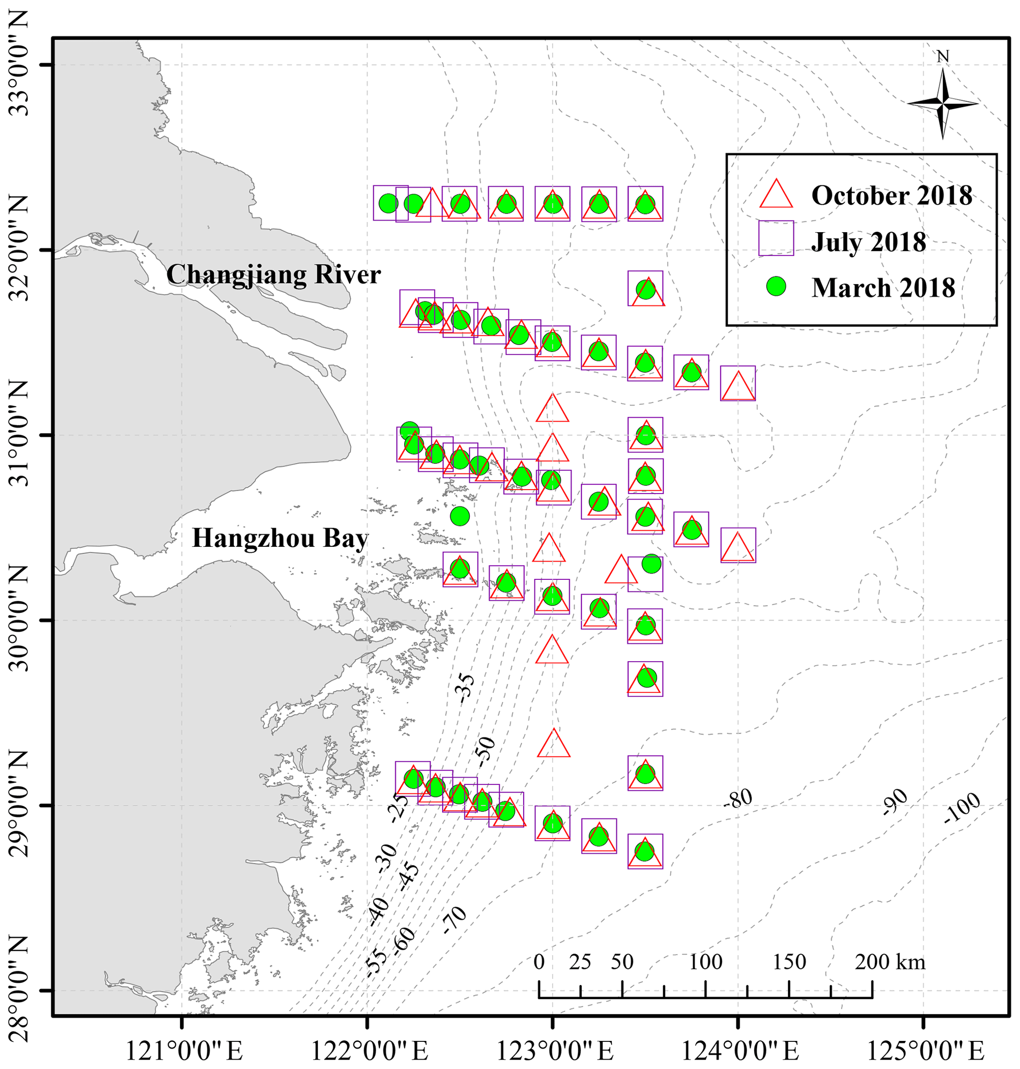
Figure 2Sampling stations for three cruises (the exploratory dataset) used to extend the utility of the ANN model. The green circles represent March 2018, the purple squares represent July 2018 and the red triangles represent October 2018.
The ECS is the largest marginal sea in the western North Pacific Ocean and receives massive terrestrial inputs from the Changjiang (Yangtze River). The shelf shallower than 200 m covers more than 70 % of the entire ECS (e.g., Ichikawa and Beardsley, 2002; Lie and Cho, 2016), where the dominant currents present seasonal circulation patterns. The spatial and temporal distributions of the carbonate system have been investigated in the ECS (e.g., Chou et al., 2009; Cao et al., 2011; Qu et al., 2015) and were found to largely reflect the distributions of various water masses. The pattern of carbon sources and sinks exhibits substantial seasonal variation (Guo et al., 2015), and the ECS is generally considered as a sink of atmospheric CO2 throughout the year except in fall (e.g., Shim et al., 2007; Zhai and Dai, 2009). A mechanistic semi-analytical algorithm (MeSAA) was developed to study pCO2 variations in response to various controlling mechanisms during summertime (Bai et al., 2015). However, the seasonal variability of pH has been studied very little in the ECS, mainly due to the limited observational coverage and irregular variability caused by seasonal fluctuations of the Changjiang discharge and anthropogenic processes. Developing methods to extend the seasonal coverage of pH data may thus help to improve our understanding of the ocean carbon cycle in the ECS.
This paper is structured as follows: Sect. 2 describes the cruise data and ANN model building; Sect. 3 shows the performance, sensitivity and application of the ANN model. A summary is given and conclusions are drawn in the last section.

Figure 3Schematic representation of the neural network algorithm to retrieve pHT. (a) The architecture of the ANN model. Input variables are observed temperature, salinity, dissolved oxygen, nitrate, phosphate and silicate together with the geolocation (longitude and latitude) and time (month) of sampling. (b) Data distribution diagram for training and prediction.
2.1 Data
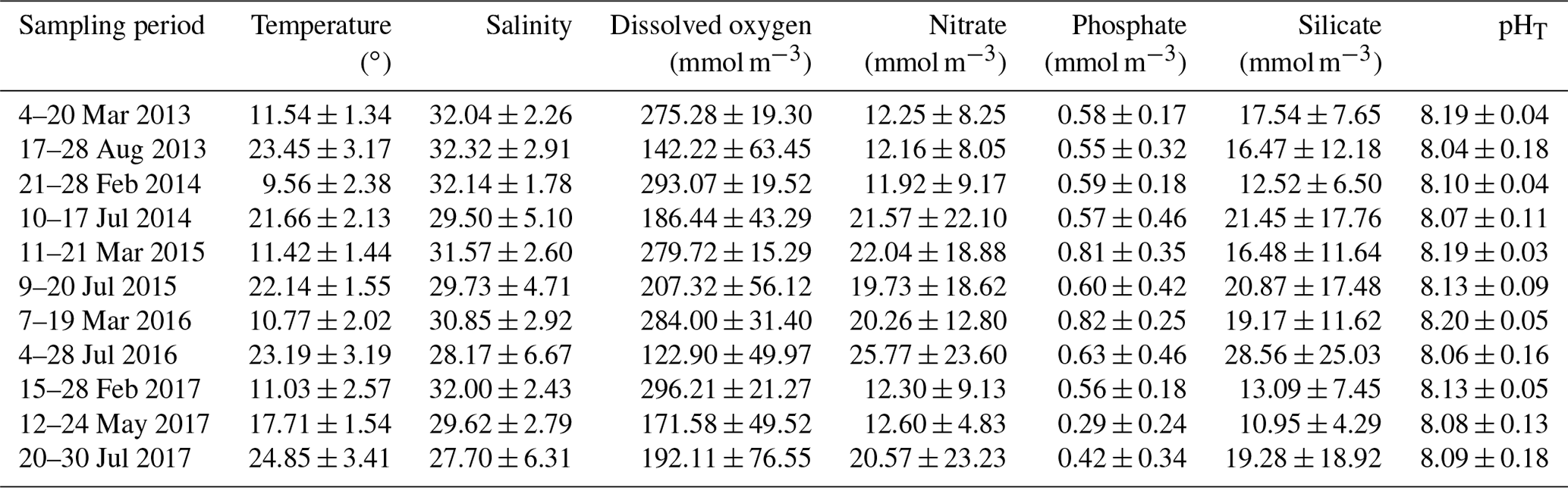
Ten cruises were conducted on the ECS shelf during the “Shiptime Sharing Project of National Natural Science Foundation of China” from 2013 to 2017 (Fig. 1): the summer cruises from 17 to 28 August 2013, 10 to 17 July 2014, 9 to 20 July 2015, 4 to 28 July 2016 and 20 to 30 July 2017; the winter cruises from 21 to 28 February 2014 and 15 to 28 February 2017; and the spring cruises from 4 to 20 March 2013, 11 to 21 March 2015 and 7 to 19 March 2016. T and S profiles were obtained directly using conductivity, temperature and depth/pressure (CTD) recorders (SBE 25plus or 911plus). Measurement of DO followed the Winkler procedure, as described previously by Zhai et al. (2014). Nutrients samples were first filtered with a 0.45 µm Whatman GF/F membrane and then stored in 250 mL high-density polyethylene (HDPE) bottles until chemical analysis. Nitrate (N), phosphate (P) and silicate (Si) were determined using a segmented flow analyzer (model: Skalar SANPLUS, Netherlands) with a precision < 5 % (Zhang et al., 2007); the detection limits are 0.14 µM for N, 0.06 µM for P and 0.07 µM for Si. pH samples were stored in 140 mL brown borosilicate glass bottles and sterilized by addition of 50 µL saturated HgCl2 solution. Three traceable pH buffers were used including NIST (National Institute of Standards and Technology) buffers with pH = 4.00, 7.02 and 10.09. As described by Zhai et al. (2012, 2014), we converted it into total-scale pH (pHT) by subtracting 0.143, and the overall accuracy of the pHT dataset was estimated as 0.01.
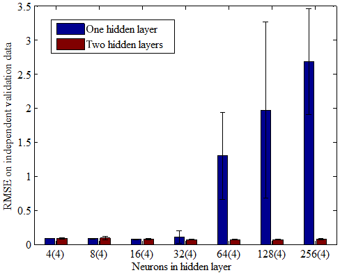
Figure 4Comparison of the performance of one hidden layer vs. two hidden layers in predicting independent validation data. The number of neurons in the first hidden layer was the same in the one-hidden-layer as in the two-hidden-layer model; numbers in parentheses show the number of neurons in the second hidden layer (for the two-hidden-layer model). Bars show the mean and standard deviation of the root mean square error over a 10-fold cross-validation, for different numbers of neurons in the first hidden layer.
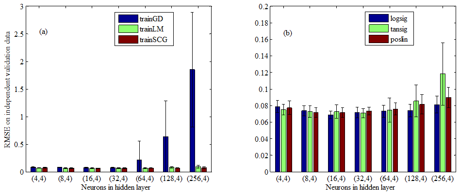
Figure 5Comparison of the performance of different training functions and transfer functions on independent validation data. (a) Three training functions: gradient descent backpropagation (trainGD), Levenberg–Marquardt backpropagation (trainLM) and scaled conjugate gradient backpropagation (trainSCG). (b) Three transfer functions: log-sigmoid transfer function (logsig), hyperbolic tangent sigmoid transfer function (tansig) and positive linear transfer function (poslin). Bars show the mean and standard deviation of the root mean square error over a 10-fold cross-validation, for different numbers of neurons in the first hidden layer.
Three cruises were carried out on the ECS shelf in 2018 (Fig. 2) during the “National Natural Science Foundation Shared Voyage Plan” – from 10 to 19 March, 12 to 20 July and 12 to 21 October – and one cruise was carried out near the Changjiang Estuary during May 2017 (Fig. 1). The measurement methods of T, S, DO and nutrients are the same as that of the above 10 voyages. pH samples were stored in 500 mL high-quality borosilicate glass bottles without filtering and sterilized by addition of 200 µL saturated HgCl2 solution until measurement in the lab. The pHT was measured at the temperature in the flow cell using an automated flow-through system for embedded spectrophotometry (AFtes) with a precision of 0.0005 pH and uncertainty of < 0.003 (Reggiani et al., 2016). Water samples were collected at three or four different depths during all cruises.
We omitted data points where one or more other physical variables were missing. The three cruises during 2018 (Fig. 2) were used to estimate model-predicted performance as an exploratory dataset, while the remaining 11 cruises (Fig. 1) were used to train the model as a confirmatory dataset. The final number of observations in the confirmatory dataset was 1854 (see Table 1 for more detailed information on the field survey).
Table 1Field survey information and measurements of water temperature, salinity, dissolved oxygen, nitrate, phosphate, silicate and pHT (mean ± SE).
2.2 Artificial neural network development
The ANN we used is a feed-forward multilayer perceptron (Tamura and Tateishi, 1997) with two hidden layers. The neurons of each layer are connected with the neurons of the previous layer and the next layer by weights (Fig. 3a). The coefficients of the weight matrix are iteratively tuned in the training step. In order to avoid overfitting, a 10-fold cross-validation was used to assess model prediction accuracy (Fig. 3b). Here, the confirmatory dataset was randomly divided into 10 equal subsamples. One subsample was used as the independent validation data (10 % of the confirmatory dataset) and was always excluded from training; the remaining nine subsamples were used as training data (90 % of the confirmatory dataset). The training data were further divided randomly into a training set (70 % of the training data), validation set (15 % of the training data) and testing set (15 % of the training data) during the training process. The training set was used for computing the gradient and updating the network weights and biases, the validation set was used to monitor the error and control model stop, and the testing set was used to monitor whether the model was over-fitted (Palacz et al., 2013). We compared performances in predicting the independent validation data from the 10-fold cross-validation and selected the optimal model based on the lowest root mean square error (RMSE). Then we applied the optimal model to the exploratory dataset (Fig. 2) and evaluated model performance by calculating error statistics. In our study, calculations were done in the MathWorks MATLAB environment, using the Deep Learning Toolbox.
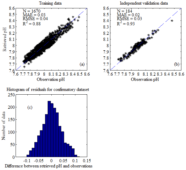
Figure 6Comparison of pHT retrieved by the ANN model with corresponding observations. (a) Training data (90 % of confirmatory dataset); (b) independent validation data (10 % of confirmatory dataset); (c) histogram of residuals for confirmatory dataset. The 1:1 line is shown in each plot as a visual reference. Three statistics are the mean absolute error (MAE), the coefficient of determination (R2) and the root mean square error (RMSE). N represents the number of data points.
First, we compared the performance of one hidden layer vs. two hidden layers in predicting independent validation data. The number of neurons varied from 22 to 28 for the first hidden layer and was fixed at four in the second hidden layer for the two-hidden-layer model; the number of neurons in the first layer was the same in the one-hidden-layer vs. two-hidden-layer model (Fig. 4). The 10-fold cross-validation showed that the model with two hidden layers performed better as the number of neurons increased. Second, in order to choose suitable training techniques and activation functions of the ANN model with two hidden layers, we tested three training functions (gradient descent backpropagation (trainGD), Levenberg–Marquardt backpropagation (trainLM) and scaled conjugate gradient backpropagation (trainSCG)), which differed in how the weights are modified, and three transfer functions (log-sigmoid transfer function (logsig), hyperbolic tangent sigmoid transfer function (tansig) and positive linear transfer function (poslin)) (Fig. 5). The output values of logsig, tansig and poslin were compressed onto [0, 1], [−1, 1] and [0, +∞], respectively (Fig. S1). As the number of neurons increased, the performances of trainGD and tansig became poor. Although there was no obvious difference between trainLM and trainSCG, the training technique trainSCG was selected and the transfer function logsig was applied to two hidden layers considering the overall performance (Fig. 5). Third, in the training phase of the ANN model, the number of neurons was tested, varying from 4 to 128 for two hidden layers (Table S1). The best performance for both training data and independent validation data was obtained with 40 neurons in the first hidden layer and 16 neurons in the second layer. Finally, different combinations of input variables were tested to choose the optimal architecture of the ANN model (Table 2); the best performance was obtained using longitude, latitude, month, T, S, DO, N, P and Si as input variables. The utility of these variables for predicting pH has a strong a priori basis: the carbonate system thermodynamic relationships depend on both T and S (Lueker et al., 2000); a positive correlation is expected between DO and pH (Wootton et al., 2012) because of the role of photosynthesis and respiration in removing or generating CO2 in the water; and various nutrients influence phytoplankton growth and abundance, thereby increasing organic carbon fixation/uptake and increasing pH (Wootton et al., 2008, 2012). We found geographical information to be a powerful addition in improving the skill of the method (Table 2), allowing the network to learn spatiotemporal patterns that could not be explained by other input variables (Sasse et al., 2013).
Table 2Different model structures and their performance in the training step. The variables (Long (longitude), Lat (latitude), Month (month), T (temperature), S (salinity), DO (dissolved oxygen), N (nitrate), P (phosphate), Si (silicate)) marked with 1 represent the input variables. Skill statistics include the coefficient of determination (R2), the root mean square error (RMSE) and the mean absolute error (MAE).

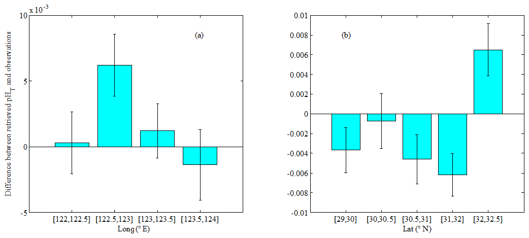
Figure 7Box plots of the differences between retrieved pHT and the observations. (a) The differences vs. longitude (mean ± SE); (b) the differences vs. latitude (mean ± SE). The height of each box represents the mean value of the differences; the whiskers represent the standard error (SE) value of the differences.
In order to avoid bias towards high-value inputs/outputs and to eliminate the dimensional influence of the data, all data used by the ANN model were normalized using the following equation (e.g., Sauzède et al., 2015, 2016):
with σ being the standard deviation of the considered input variables or output variable pHT. Similar to the approach of Sauzède et al. (2015, 2016), the longitude and month input variables were transformed as follows to account for the periodicity:
The latitude variable was transformed into the range of the sigmoid function by dividing by 90 and then normalized using Eq. (1).

Figure 8Comparison of retrieved pHT with corresponding observations for exploratory dataset. (a) pHT retrieved by the ANN model vs. observations; (b) pHT retrieved by CANYON (Sauzède et al., 2017) vs. observations. The red circles represent March 2018, the blue squares represent July 2018 and the green triangles represent October 2018. The 1:1 line is shown in the plot as a visual reference. Three statistics approaches used are the mean absolute error (MAE), the root mean square error (RMSE) and the coefficient of determination (R2). N represents the number of data points.
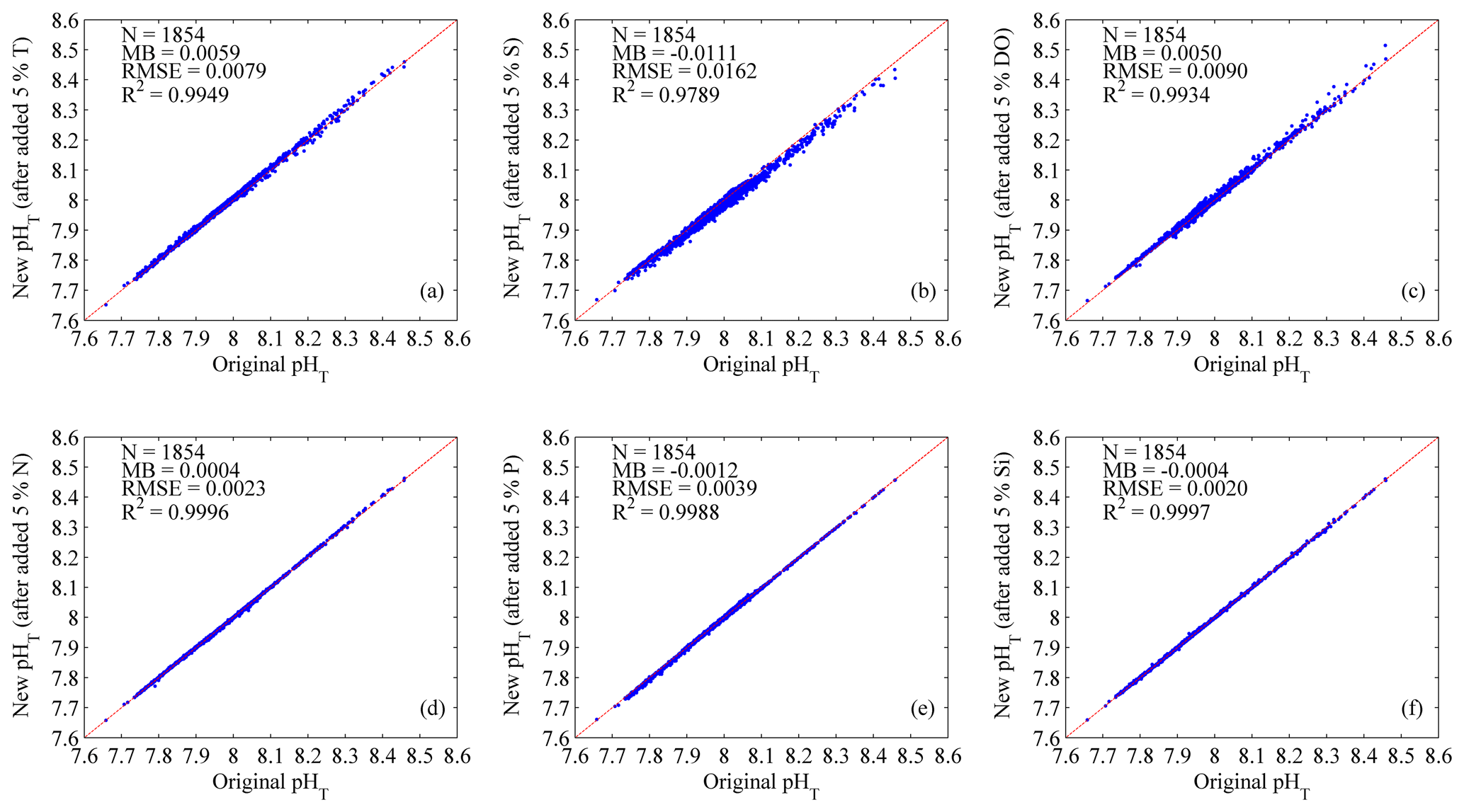
Figure 9Sensitivity of the ANN model for environmental input variables. (a) Temperature (T); (b) salinity (S); (c) dissolved oxygen (DO); (d) nitrate (N); (e) phosphate (P); (f) silicate (Si). Three statistics approaches used are the mean bias (MB), the root mean square error (RMSE) and the coefficient of determination (R2). N represents the number of data points.
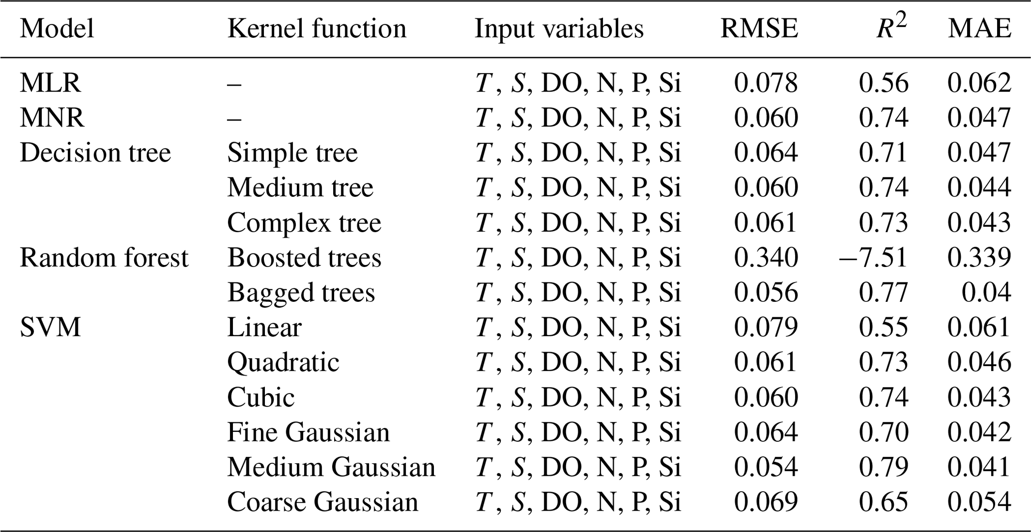
Table 3Model comparison between traditional empirical methods (MLR and MNR) and machine-learning-based empirical methods (decision tree, random forest and SVM). The statistics was derived from the confirmatory dataset (training data and independent validation data) using input variables: T, S, DO, N, P and Si. Note that R2 statistics in our study were based on the calculation of the coefficient of determination; therefore negative R2 could be derived when there was a strong bias.
3.1 ANN model performance
To evaluate the performance of the ANN model, we compared model-simulated pHT (pH) with corresponding observations (pH) using several statistical indices, including the mean absolute error (MAE), the coefficient of determination (R2) and the RMSE. The model simulated pHT with a RMSE of 0.04 and R2 of 0.88 for the training data (90 % of confirmatory dataset, Fig. 6a), and predicted pHT with a RMSE of 0.03 and R2 of 0.93 for the independent validation data (10 % of confirmatory dataset, Fig. 6b). The histogram of residuals in the confirmatory dataset (Fig. 6c) showed that 68 % of the residuals were within the RMSE of 0.04. In order to further explore where the ANN model may lead to large errors, we plotted distributions of differences (pH–pH) with respect to the longitude and latitude (Fig. 7). The points with large errors are mainly concentrated in the longitude range [122.5, 123∘ E] and the latitude range [31, 32.5∘ N], in an area strongly influenced by the Changjiang Diluted Water (CDW). The reduced performance of the ANN model here may be primarily due to the strong seasonal oscillations of the Changjiang discharge (Dai and Trenberth, 2002). As a reference, the performance of some other empirical approaches – including MLR, multi-variate nonlinear regression (MNR), decision tree, random forest and support vector machine (SVM) regression – is shown in Table 3. The selected ANN model (Table 2, model no. 10) showed better performance than the other tested approaches using the same input variables (Table 3).
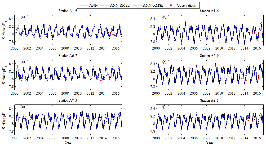
Figure 10Comparison of surface pHT retrieved by the ANN model using Changjiang biology FVCOM output with corresponding observations at six sites with repeated sampling for 3 to 4 years. Red dots represent observed pHT, solid blue line represents retrieved pHT, and dotted black lines represent upper and lower bounds of the ANN model accuracy (ANN ± RMSE). (a) Station A1-5; (b) station A1-6; (c) station A6-7; (d) station A6-9; (e) station A7-5; (f) station A8-5.
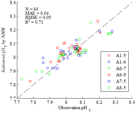
Figure 11Comparison of water column pHT retrieved by the ANN model using Changjiang biology FVCOM output with corresponding observations at six sites with repeated sampling for 3 to 4 years. The 1:1 line is shown in the plot as a visual reference. Skill statistics include the mean absolute error (MAE), the coefficient of determination (R2) and the root mean square error (RMSE). N represents the number of data points.
3.2 ANN model validation using the exploratory dataset
To further assess the ability of the ANN model to estimate pHT on the ECS shelf, we applied the ANN model to an exploratory dataset not used in ANN model development and sampled during March, July and October 2018 (Fig. 2). Scatterplots of retrieved pHT vs. observations (Fig. 8a) showed a RMSE of 0.04, R2 of 0.80 and MAE of 0.03, which is consistent with the performance of the training data (Fig. 6a). Although the RMSE for pHT we obtained here was higher than obtained in some previous studies (e.g., Juranek et al., 2011; Williams et al., 2016; Sauzède et al., 2017), these latter studies considered open-ocean regions, not coastal seas. For example, Juranek et al. (2011) developed empirical algorithms to estimate pH with a RMSE of 0.018 for data between 30 and 500 m in the NE subarctic Pacific, Williams et al. (2016) also developed empirical algorithms to predict pH with a RMSE of 0.01 in the Southern Ocean and Sauzède et al. (2017) developed a neural network method to estimate pH with a RMSE of 0.02 in the global ocean. As a further comparison we applied the CANYON model developed by Sauzède et al. (2017) to our coastal exploratory dataset (Fig. 8b) and obtained a RMSE of 0.09 and MAE of 0.06. It is not surprising that the ANN model (developed here for the ECS shelf) outperforms the CANYON model (developed for the global ocean) for predicting pHT on the ECS shelf. The carbon chemistry parameters in this region are not only under the direct impact of the Taiwan Warm Current and remote control of the Kuroshio water intrusion into the shelf, but they are also significantly controlled by seasonal variations of the Changjiang discharge (e.g., Isobe and Matsuno, 2008; Chen et al., 2008; Chou et al., 2009). Taking into account the highly complex hydrographic, biological and chemical conditions, the accuracy of pHT presented is promising.
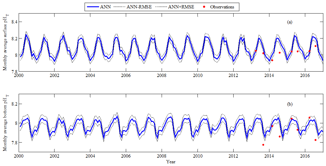
Figure 12Comparison of monthly average pHT on the East China Sea shelf. Solid blue line represents retrieved pHT by the ANN model using Changjiang biology FVCOM output, dotted black lines represent upper and lower bounds of the ANN model accuracy (ANN ± RMSE), and red points show monthly average pHT observations from 2013 to 2016. (a) Surface; (b) bottom.
3.3 ANN model sensitivity to environmental input variables
To assess the ANN model sensitivity to different environmental input variables, we added 5 % perturbation for each environmental variable separately. Statistically, with 5 % T errors added, the ANN model showed slight overestimation in pHT, with a mean bias (MB) of 0.0059, RMSE of 0.0079 and R2 of 0.9949 (Fig. 9a); with 5 % DO errors added, the ANN model also showed slight pHT overestimation, with a MB of 0.0050, RMSE of 0.0090 and R2 of 0.9934 (Fig. 9c); and with 5 % S errors added, the ANN model showed an overestimation in pHT, with a MB of −0.0111, RMSE of 0.0162 and R2 of 0.9789 (Fig. 9b). These results suggested that the ANN model responded to T and DO errors in a positive way and to S errors in a negative way. The positive response to increasing DO reflects a positive correlation between pHT and DO (Cai et al., 2011), which can be attributed to the processes of photosynthesis (generating DO and removing CO2, hence increasing pH) and aerobic respiration (consuming DO and generating CO2, hence lowering pH); the negative response to increasing S reflects the influence of the (lower-salinity) Changjiang discharge, carrying large amounts of nutrients that fuel increased primary production (uptake of nutrients and CO2, hence raising the pH) in surface waters during warm seasons (Gong et al., 2011). It was found that the ANN model was insensitive to nutrient errors (Fig. 9d–f) and most sensitive to S errors (Fig. 9b), followed by DO and T errors.
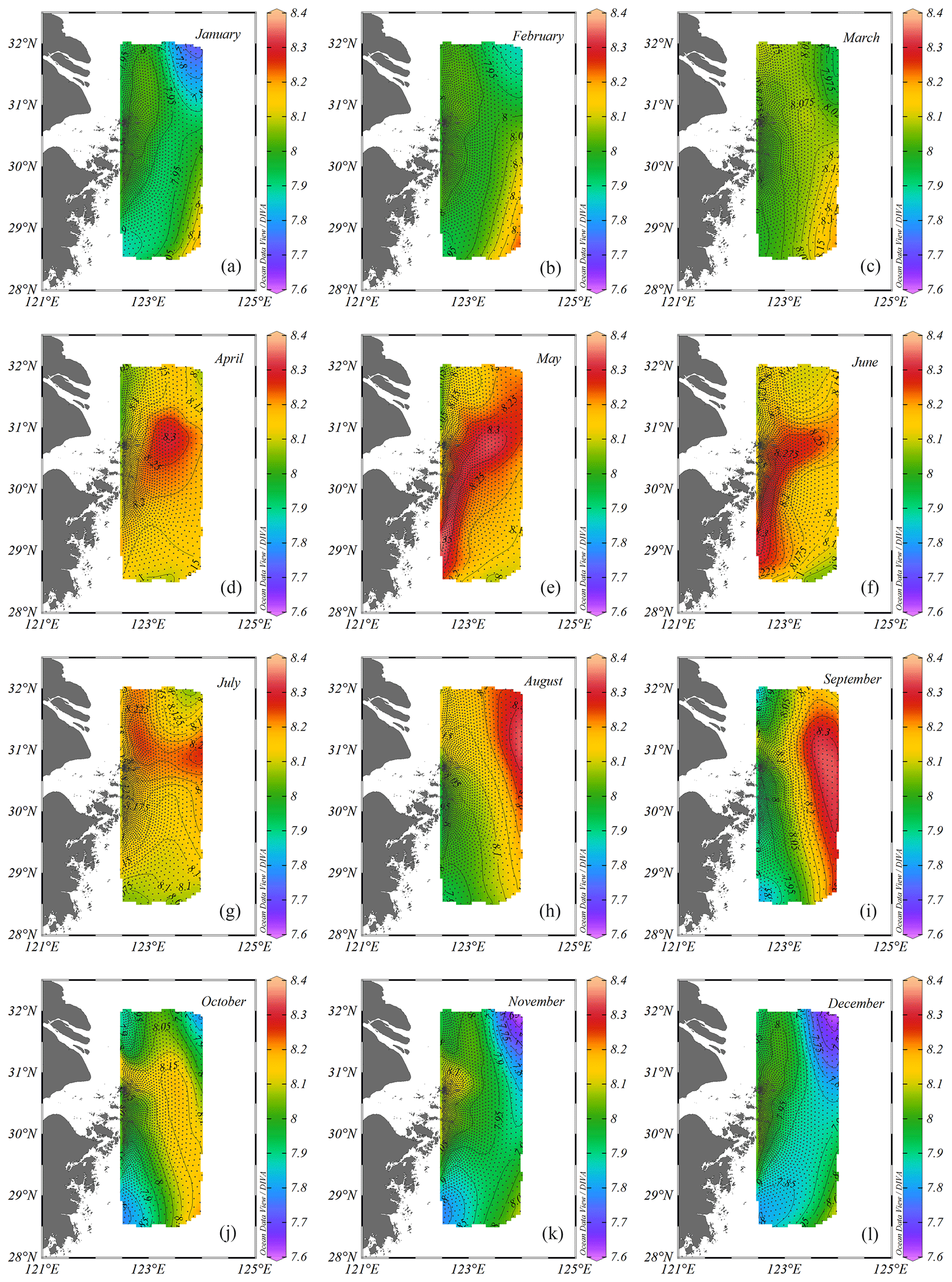
Figure 13Spatial distribution of monthly average surface pHT retrieved by the ANN model using Changjiang biology FVCOM output. (a) January; (b) February; (c) March; (d) April; (e) May; (f) June; (g) July; (h) August; (i) September; (j) October; (k) November; (l) December.
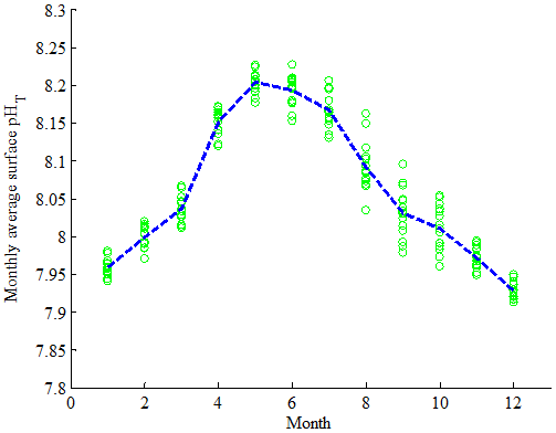
Figure 14Seasonal cycles of surface pHT on the East China Sea shelf from 2000 to 2016. The green circles represent the monthly regional average; the dashed blue line represents the mean value of each month.
3.4 ANN model application
3.4.1 Comparison
In order to retrieve monthly pHT on the ECS shelf, the monthly T, S, DO, N, P and Si from the Changjiang biology Finite-Volume Coastal Ocean Model (FVCOM) (http://47.101.49.44/wms/demo, last access: 20 July 2018) were fed into the ANN model as input variables. The resolution of the Changjiang biology FVCOM output is 1–10 km in the horizontal, 10 depth levels in the vertical and day in the temporal (refer to Ge et al., 2013, for detail information). Comparisons of monthly average FVCOM variables with surface and bottom observations on the ECS shelf showed that simulated T was close to observed values (Fig. S2a), simulated S was also close to observed values except at the bottom in August 2013 and at the surface in July 2016 (Fig. S2b), simulated DO was higher than observed at the bottom (Fig. S2c), and simulated nutrients were higher than observed at the surface (Fig. S2d–f). Comparisons of monthly average pHT from the FVCOM biogeochemical model with pHT retrieved by the ANN model suggested that the ANN model can potentially provide a more accurate pHT (Fig. S3). The possible reason was that the carbonate system from the Changjiang biology FVCOM was not optimized due to challenges obtaining sufficient boundary information.
Considering the discreteness and discontinuity of the sampling sites, we compared pHT retrieved by the ANN model using the Changjiang biology FVCOM output with the corresponding observations at some sites with repeated sampling for 3 to 4 years. These sites were A1-5 (32.2145∘ N, 123.0140∘ E), A1-6 (32.2679∘ N, 123.2750∘ E), A6-7 (30.7050∘ N, 122.9880∘ E), A6-9 (30.5723∘ N, 123.4990∘ E), A7-5 (30.2523∘ N, 123.4990∘ E) and A8-5 (29.9940∘ N, 123.4930∘ E). Overall, the retrieved pHT agrees well (within the ANN model accuracy: ANN ± RMSE) with the observed values at the surface, except for three samples in summer (Fig. 10). There are relatively large deviations (greater than the RMSE of 0.04) in August 2013 at stations A1-5 and A6-9, and in July 2016 at station A8-5. To illustrate the application performance in the water column, a scatterplot of retrieved pHT vs. observations at six sites with repeated sampling for 3 to 4 years (Fig. 11) showed that the ANN model predicted pHT with a RMSE of 0.05 and R2 of 0.71.
We further compared monthly pHT retrieved by the ANN model using the Changjiang biology FVCOM output with in situ measured pHT values (Fig. 12). The agreement is good (within the ANN model accuracy: ANN ± RMSE) here in winter, but large deviations (greater than the RMSE of 0.04) appear in summer. The reduced performance in summer can be attributed in large part to a reduced performance of the Changjiang biology FVCOM in predicting summertime input variables S and DO, and nutrients (Fig. S2).
3.4.2 Spatial and temporal patterns of ANN-derived pHT
The temporal and spatial variations of monthly surface pHT from 2000 to 2016 based on Changjiang biology FVCOM output are shown in Fig. 13. During the dry season (November to March of the next year), pHT values vary from ∼ 7.62 to ∼ 8.24. Relatively higher pHT values are found in the southeast of the study area (Chou et al., 2011), whereas lower pHT values are found in the northeast of the study area. During the wet season (April to October), pHT values vary from ∼ 7.77 to ∼ 8.35, and water of higher pHT corresponds well to the seasonal dispersion of the Changjiang Diluted Water (Chou et al., 2009, 2013). Water of higher pHT is found in the center of the study area during April, spreads to the southwestern part of the study area (along the coast of China) during May and June, and shifts to the northeastern part of the study area during August. In September and October, water of higher pHT is found in the southeastern part of the study area, strongly influenced by the Taiwan Warm Current (Qu et al., 2015).
A clear seasonality is that surface pHT gradually increases during spring (March to May), after which it gradually decreases during summer and fall (June to November) (Fig. 14). The surface pHT displays its maximum in May and minimum in December, and the pHT varies seasonally by up to ∼ 0.3. Larger changes in pH were also discovered on the Washington shelf; the pH varied ∼ 1.0 over the seasons and ∼ 1.5 spanning 8 years (Wootton et al., 2008). Accordingly, seasonal dynamics of surface pHT can be mainly attributed to temperature changes and strong biological activities (production and respiration processes) over the season. From March to June, a rapid increase in surface pHT indicates that production increases faster than respiration, which can be reflected in the drop in surface phosphate (Fig. S5d) and apparent oxygen utilization (AOU) (Fig. S5c). It may be driven by the Changjiang discharge (Fig. S4), which carries large amount of nutrients, resulting in stronger primary production in warm seasons under the combined action of nutrients and suitable temperature (Gong et al., 2011). From July to October, although surface temperature remains at a high level (Fig. S5a), the rise in surface AOU (Fig. S5c) suggests a decrease in primary production or increase of respiration, which leads to a gradual drop in surface pHT (Wootton et al., 2012). It implies that respiration processes dominate relative to primary production during summer and fall.
We have developed an artificial neural network (ANN) model, demonstrated its reliability and used it to retrieve monthly pHT for the period 2000–2016 on the East China Sea shelf. We trained this ANN model using 11 cruise datasets from 2013 to 2017. In order to choose the optimal architecture of the ANN model, we tested different training and transfer functions, the number of neurons in two hidden layers and different combinations of input variables. We also validated the reliability of the ANN model with a root mean square error accuracy of 0.04 using three cruises in 2018 as an exploratory dataset. The ANN model responded to temperature and dissolved oxygen errors in a positive way and to salinity errors in a negative way, and it was most sensitive to salinity errors, followed by dissolved oxygen and temperature errors. We also retrieved monthly average pHT using the ANN model in combination with input variables from the Changjiang biology Finite-Volume Coastal Ocean Model (FVCOM).
The approach has several potential applications. First, it can provide estimates of seawater pHT with known accuracies for the East China Sea shelf and the period 2013–2018. Within this region the model could be used as a cost-effective way to handle restrictions of marine observations conducted from ships, such as coarse resolution and undersampling of carbonate system variables. Second, while the ANN model is not a replacement for direct measurements of the carbonate system, it may be a valuable tool for understanding the seasonal variation of pHT in poorly observed regions. Third, this approach can be applied to other regions to predict pH by suitably adapting the input variables and network structure using a local dataset. The MATLAB code used in this study to develop and apply the ANN model is freely available and is accompanied by a README file providing detailed guidance on how to use and adapt the code.
MATLAB code of the ANN model for pHT estimation and datasets are available at https://doi.org/10.5281/zenodo.3519219 (Li, 2019a). The monthly average input variables (T, S, DO, N, P, Si) from the Changjiang biology Finite-Volume Coastal Ocean Model, retrieved pHT values from 2000 to 2016 on the East China Sea shelf and the data from three cruises during 2018 used to evaluate the ANN model are available at https://doi.org/10.5281/zenodo.3519236 (Li, 2019b). Requests to access the raw data should be directed to Richard Bellerby: richard.bellerby@niva.no. Six stations with repeated sampling for 3 to 4 years and corresponding retrieved pH values from the Changjiang biology FVCOM output are available at https://doi.org/10.5281/zenodo.3491747 (Li, 2019c).
Monthly distribution of surface pHT on the East China Sea shelf from 2000 to 2016: https://doi.org/10.5281/zenodo.2672943 (Li, 2019d). Profile distribution of pHT at 31∘ N on the East China Sea shelf from 2000 to 2016: https://doi.org/10.5281/zenodo.2672929 (Li, 2019e).
The supplement related to this article is available online at: https://doi.org/10.5194/gmd-13-5103-2020-supplement.
XL, PW, and RGJB contributed to the development of methodology and the design of the model. JG provided 10 cruise datasets from 2013 to 2017 and the input variables from the Changjiang biology Finite-Volume Coastal Ocean Model data. JL and AY provided four cruise datasets from 2017 to 2018. XL developed the manuscript with contributions from all co-authors.
The authors declare that they have no conflict of interest.
This study was financially supported by the National Thousand Talents Program for Foreign Experts (grant no. WQ20133100150), Vulnerabilities and Opportunities of the Coastal Ocean (grant no. SKLEC-2016RCDW01), Marginal Seas (MARSEAS) (grant SKLEC-Taskteam project) and Innovative Talents International Cooperation Training Project (grant no. China Scholarship Council-201913045). Richard Bellerby and Philip Wallhead were also supported by funding from the FRAM High North Research Centre for Climate and the Environment under the Ocean Acidification Flagship and the NIVA Land-Ocean Interactions Strategic Institute program. We deeply thank the people who worked on the cruises and in the laboratory.
This research has been supported by the Vulnerabilities and Opportunities of the Coastal Ocean (grant no. 44KZ001P/015).
This paper was edited by David Ham and reviewed by Richard Mills and Jitendra Kumar.
Alin, S. R., Feely, R. A., Dickson, A. G., Hernández-Ayón, J. M., Juranek, L. W., Ohman, M. D., and Goericke, R.: Robust empirical relationships for estimating the carbonate system in the southern California Current System and application to CalCOFI hydrographic cruise data (2005–2011), J. Geophys. Res., 117, C05033, https://doi.org/10.1029/2011JC007511, 2012.
Bai, Y., Cai, W. J., He, X. Q., Zhai, W. D., Pan, D., Dai, M. H., and Yu, P. S.: A mechanistic semi-analytical method for remotely sensing sea surface pCO2 in river-dominated coastal oceans: A case study from the East China Sea, J. Geophys. Res.-Ocean., 120, 2331–2349, https://doi.org/10.1002/2014JC010632, 2015.
Bates, N. R., Astor, Y. M., Church, M. J., Currie, K., Dore, J. E., González-Dávila, M., Lorenzoni, L., Muller-Karger, F., Olafsson, J., and Santana-Casiano, J. M.: A time-series view of changing ocean chemistry due to ocean uptake of anthropogenic CO2 and ocean acidification, Oceanography, 27, 126–141, https://doi.org/10.5670/oceanog.2014.16, 2014.
Bostock, H. C., Mikaloff Fletcher, S. E., and Williams, M. J. M.: Estimating carbonate parameters from hydrographic data for the intermediate and deep waters of the Southern Hemisphere oceans, Biogeosciences, 10, 6199–6213, https://doi.org/10.5194/bg-10-6199-2013, 2013.
Cai, W. J., Hu, X. P., Huang W. J., Murrell, M. C., Lehrter, J. C., Lohrenz, S. E., Chou, W. C., Zhai, W. D., Hollibaugh, J. T., Wang, Y. C., Zhao, P. S., Guo, X. H., Gundersen, K., Dai, M. H., and Gong, G. C.: Acidification of subsurface coastal waters enhanced by eutrophication, Nat. Geosci., 4, 766–770, https://doi.org/10.1038/NGEO1297, 2011.
Cao, Z. M., Dai, M. H., Zheng, N., Wang, D., Li, Q., Zhai, W. D., Meng, F. F., and Gan, J. P.: Dynamics of the carbonate system in a large continental shelf system under the influence of both a river plume and coastal upwelling, J. Geophys. Res., 116, G02010, https://doi.org/10.1029/2010JG001596, 2011.
Carter, B. R., Williams, N. L., Gray, A. R., and Feely, R. A.: Locally interpolated alkalinity regression for global alkalinity estimation, Limnol. Oceanogr.-Meth., 14, 268–277, https://doi.org/10.1002/lom3.10087, 2016.
Carter, B. R., Feely, R. A., Williams, N. L., Dickson, A. G., Fong, M. B., and Takeshita, Y.: Updated methods for global locally interpolated estimation of alkalinity, pH, and nitrate, Limnol. Oceanogr.-Meth., 16, 119–131, https://doi.org/10.1002/lom3.10232, 2018.
Chen, C. S., Xue, P. F., Ding, P. X., Beardsley, R. C., Xu, Q. C., Mao, X. M., Gao, G. P., Qi, J. H., Li, C. Y., Lin, H. C., Cowles, G., and Shi, M. C.: Physical mechanisms for the offshore detachment of the Changjiang Diluted Water in the East China Sea, J. Geophys. Res., 113, C02002, https://doi.org/10.1029/2006JC003994, 2008.
Chen, S. L. and Hu, C. M.: Estimating sea surface salinity in the northern Gulf of Mexico from satellite ocean color measurements, Remote Sens. Environ., 201, 115–132, https://doi.org/10.1016/j.rse.2017.09.004, 2017.
Chou, W. C., Gong, G. C., Sheu, D. D., Hung, C. C., and Tseng, T. F.: Surface distributions of carbon chemistry parameters in the East China Sea in summer 2007, J. Geophys. Res., 114, C07026, https://doi.org/10.1029/2008JC005128, 2009.
Chou, W. C., Gong, G. C., Tseng, C. M., Sheu, D. D., Hung, C. C., Chang, L. P., and Wang, L. W.: The carbonate system in the East China Sea in winter, Mar. Chem., 123, 44–55, https://doi.org/10.1016/j.marchem.2010.09.004, 2011.
Chou, W. C., Gong, G. C., Hung, C. C., and Wu, Y. H.: Carbonate mineral saturation states in the East China Sea: present conditions and future scenarios, Biogeosciences, 10, 6453–6467, https://doi.org/10.5194/bg-10-6453-2013, 2013.
Ciais, P., Sabine, C., Bala, G., Bopp, L., Brovkin, V., Canadell, J., Chhabra, A., DeFries, R., Galloway, J., Heimann, M., Jones, C., Le Quéré, C., Myneni, R. B., Piao, S., and Thornton, P.: Carbon and Other Biogeochemical Cycles, in: Climate Change 2013: The Physical Science Basis. Contribution of Working Group I to the Fifth Assessment Report of the Intergovernmental Panel on Climate Change, edited by: Stocker, T. F., Qin, D., Plattner, G. K., Tignor, M., Allen, S. K., Boschung, J., Nauels, A., Xia, Y., Bex, V., and Midgley, P. M., Cambridge University Press, Cambridge, United Kingdom and New York, NY, USA, 465–570, 2014.
Dai, A. and Trenberth, K. E.: Estimates of freshwater discharge from continents: Latitudinal and seasonal variations, J. Hydrometeorol., 3, 660–687, 2002.
Dore, J., Lukas, R., Sadler, D., Church, M., and Karl, D.: Physical and biogeochemical modulation of ocean acidification in the central North Pacific, P. Natl. Acad. Sci. USA, 106, 12235–12240, 2009.
Friedrich, T. and Oschlies, A.: Neural network-based estimates of North Atlantic surface pCO2 from satellite data: A methodological study, J. Geophys. Res., 114, C03020, https://doi.org/10.1029/2007JC004646, 2009.
Ge, J. Z., Ding, P. X., Chen, C. S., Hu, S., Fu, G., and Wu, L. Y.: An integrated East China Sea–Changjiang Estuary model system with aim at resolving multi-scale regional–shelf–estuarine dynamics, Ocean Dynam., 63, 881–900, https://doi.org/10.1007/s10236-013-0631-3, 2013.
Gong, G. C., Liu, K. K., Chiang, K. P., Hsiung, T. M., Chang, J., Chen, C. C., Hung, C. C., Chou, W. C., Chung, C. C., Chen, H. Y., Shiah, F. K., Tsai, A. Y., Hsieh, C. H., Shiao, J. C., Tseng, C. M., Hsu, S. C., Lee, H. J., Lee, M. A., Lin, I. I., and Tsai, F.: Yangtze River floods enhance coastal ocean phytoplankton biomass and potential fish production, Geophys. Res. Lett., 38, L13603, https://doi.org/10.1029/2011GL047519, 2011.
González-Dávila, M., Santana-Casiano, J. M., Rueda, M. J., and Llinás, O.: The water column distribution of carbonate system variables at the ESTOC site from 1995 to 2004, Biogeosciences, 7, 3067–3081, https://doi.org/10.5194/bg-7-3067-2010, 2010.
Guo, X. H., Zhai, W. D., Dai, M. H., Zhang, C., Bai, Y., Xu, Y., Li, Q., and Wang, G. Z.: Air–sea CO2 fluxes in the East China Sea based on multiple-year underway observations, Biogeosciences, 12, 5495–5514, https://doi.org/10.5194/bg-12-5495-2015, 2015.
Ichikawa, H. and Beardsley, R. C.: The Current System in the Yellow and East China Seas, J. Oceanogr., 58, 77–92, https://doi.org/10.1023/A:1015876701363, 2002.
Isobe, A. and Matsuno, T.: Long-distance nutrient-transport process in the Changjiang River plume on the East China Sea shelf in summer, J. Geophys. Res.-Ocean., 113, C04006, https://doi.org/10.1029/2007JC004248, 2008.
Juranek, L. W., Feely, R. A., Gilbert, D., Freeland, H., and Miller, L. A.: Real-time estimation of pH and aragonite saturation state from Argo profiling floats: Prospects for an autonomous carbon observing strategy, Geophys. Res. Lett., 38, L17603, https://doi.org/10.1029/2011GL048580, 2011.
Laruelle, G. G., Landschützer, P., Gruber, N., Tison, J. L., Delille, B., and Regnier, P.: Global high-resolution monthly pCO2 climatology for the coastal ocean derived from neural network interpolation, Biogeosciences, 14, 4545–4561, https://doi.org/10.5194/bg-14-4545-2017, 2017.
Lauvset, S. K., Gruber, N., Landschützer, P., Olsen, A., and Tjiputra, J.: Trends and drivers in global surface ocean pH over the past 3 decades, Biogeosciences, 12, 1285–1298, https://doi.org/10.5194/bg-12-1285-2015, 2015.
Le Quéré, C., Andrew, R. M., Friedlingstein, P., Sitch, S., Hauck, J., Pongratz, J., Pickers, P. A., Korsbakken, J. I., Peters, G. P., Canadell, J. G., Arneth, A., Arora, V. K., Barbero, L., Bastos, A., Bopp, L., Chevallier, F., Chini, L. P., Ciais, P., Doney, S. C., Gkritzalis, T., Goll, D. S., Harris, I., Haverd, V., Hoffman, F. M., Hoppema, M., Houghton, R. A., Hurtt, G., Ilyina, T., Jain, A. K., Johannessen, T., Jones, C. D., Kato, E., Keeling, R. F., Goldewijk, K. K., Landschützer, P., Lefèvre, N., Lienert, S., Liu, Z., Lombardozzi, D., Metzl, N., Munro, D. R., Nabel, J. E. M. S., Nakaoka, S., Neill, C., Olsen, A., Ono, T., Patra, P., Peregon, A., Peters, W., Peylin, P., Pfeil, B., Pierrot, D., Poulter, B., Rehder, G., Resplandy, L., Robertson, E., Rocher, M., Rödenbeck, C., Schuster, U., Schwinger, J., Séférian, R., Skjelvan, I., Steinhoff, T., Sutton, A., Tans, P. P., Tian, H., Tilbrook, B., Tubiello, F. N., van der Laan-Luijkx, I. T., van der Werf, G. R., Viovy, N., Walker, A. P., Wiltshire, A. J., Wright, R., Zaehle, S., and Zheng, B.: Global Carbon Budget 2018, Earth Syst. Sci. Data, 10, 2141–2194, https://doi.org/10.5194/essd-10-2141-2018, 2018.
Li, X.: Source code of the ANN model for pH estimation, Zenodo, https://doi.org/10.5281/zenodo.3519219, last access: 25 October 2019a.
Li, X.: The monthly-average input variables (T, S, DO, N, P, Si) and retrieved pH, Zenodo, https://doi.org/10.5281/zenodo.3519236, last access: 25 October 2019b.
Li, X.: The application performance of the ANN model in the ECS shelf, Zenodo, https://doi.org/10.5281/zenodo.3491747, last access: 16 October 2019c.
Li, X.: Monthly distribution of surface pH in the East China Sea Shelf from 2000 to 2016 year, Zenodo, https://doi.org/10.5281/zenodo.2672943, last access: 7 May 2019d.
Li, X.: Profile distribution of pH at 31N in the East China Sea Shelf from 2000 to 2016 year, Zenodo, https://doi.org/10.5281/zenodo.2672929, last access: 7 May 2019e.
Lie, H. J. and Cho, C. H.: Seasonal circulation patterns of the Yellow and East China Seas derived from satellite-tracked drifter trajectories and hydrographic observations, Prog. Oceanogr., 146, 121–141, https://doi.org/10.1016/j.pocean.2016.06.004, 2016.
Lueker, T. J., Dickson, A. G., and Keeling, C. D.: Ocean pCO2 calculated from dissolved inorganic carbon, alkalinity, and equations for K1 and K2: Validation based on laboratory measurements of CO2 in gas and seawater at equilibrium, Mar. Chem., 70, 105–119, https://doi.org/10.1016/S0304-4203(00)00022-0, 2000.
Moore-Maley, B. L., Allen, S. E., and Ianson, D.: Locally driven interannual variability of near-surface pH and ΩA in the Strait of Georgia, J. Geophys. Res.-Ocean., 121, 1600–1625, https://doi.org/10.1002/2015JC011118, 2016.
Olden, J. D. and Jackson, D. A.: Illuminating the “black box”: a randomization approach for understanding variable contributions in artificial neural networks, Ecol. Model, 154, 135–150, https://doi.org/10.1016/S0304-3800(02)00064-9, 2002.
Olden, J. D., Joy, M. K., and Death, R. G.: An accurate comparison of methods for quantifying variable importance in artificial neural networks using simulated data, Ecol. Model, 178, 389–397, https://doi.org/10.1016/j.ecolmodel.2004.03.013, 2004.
Palacz, A. P., John, M. A. S., Brewin, R. J. W., Hirata, T., and Gregg, W. W.: Distribution of phytoplankton functional types in high-nitrate, low-chlorophyll waters in a new diagnostic ecological indicator model, Biogeosciences, 10, 8103–8157, https://doi.org/10.5194/bgd-10-8103-2013, 2013.
Qu, B. X., Song, J. M., Yuan, H. M., Li, X. G., Li, N., Duan, L. Q., Chen, X., and Lu, X.: Summer carbonate chemistry dynamics in the Southern Yellow Sea and the East China Sea: Regional variations and controls, Cont. Shelf Res, 111, 250–261, https://doi.org/10.1016/j.csr.2015.08.017, 2015.
Raitsos, D. E., Lavender, S. J., Maravelias, C. D., Haralabous, J., Richardson, A. J., and Reid, P. C.: Identifying four phytoplankton functional types from space: an ecological approach, Limnol. Oceanogr., 53, 605–613, https://doi.org/10.4319/lo.2008.53.2.0605, 2008.
Reggiani, E. R., King, A. L., Norli, M., Jaccard, P., Sorensen, K., and Bellerby, R. G. J.: FerryBox-assisted monitoring of mixed layer pH in the Norwegian Coastal Current, J. Mar. Syst., 162, 29–36, https://doi.org/10.1016/j.jmarsys.2016.03.017, 2016.
Sabine, C. L., Feely, R. A., Gruber, N., Key, R. M., Lee, K., Bullister, J. L., Wanninkhof, R., Wong, C. S., Wallace, D. W. R., Tilbrook, B., Millero, F. J., Peng, T. H., Kozyr, A., Ono, T., and Rios, A. F.: The oceanic sink for anthropogenic CO2, Science, 305, 367–371, 2004.
Sasse, T. P., McNeil, B. I., and Abramowitz, G.: A novel method for diagnosing seasonal to inter-annual surface ocean carbon dynamics from bottle data using neural networks, Biogeosciences, 10, 4319–4340, https://doi.org/10.5194/bg-10-4319-2013, 2013.
Sauzède, R., Claustre, H., Jamet, C., Uitz, J., Ras, J., Mignot, A., and D'Ortenzio, F.: Retrieving the vertical distribution of chlorophyll-a concentration and phytoplankton community composition from in situ fluorescence profiles: a method based on a neural network with potential for global-scale applications, J. Geophys. Res.-Ocean., 120, 451–470, https://doi.org/10.1002/2014JC010355, 2015.
Sauzède, R., Claustre, H., Uitz, J., Jamet, C., Dall'Olmo, G., D'Ortenzio, F., Gentili, B., Poteau, A., and Schmechtig, C.: A neural network-based method for merging ocean color and Argo data to extend surface bio-optical properties to depth: retrieval of the particulate backscattering coefficient, J. Geophys. Res.-Ocean., 121, 2552–2571, https://doi.org/10.1002/2015JC011408, 2016.
Sauzède, R., Bittig, H. C., Claustre, H., de Fommervault, O. P., Gattuso, J. P., Legendre, L., and Johnson, K. S.: Estimates of Water-Column Nutrient Concentrations and Carbonate System Parameters in the Global Ocean: A Novel Approach Based on Neural Networks, Front. Mar. Sci., 4, 128, https://doi.org/10.3389/fmars.2017.00128, 2017.
Shim, J. H., Kim, D., Kang, Y. C., Lee, J. H., Jang, S. T., and Kim, C. H.: Seasonal variations in pCO2 and its controlling factors in surface seawater of the northern East China Sea, Cont. Shelf Res., 27, 2623–2636, https://doi.org/10.1016/j.csr.2007.07.005, 2007.
Tamura, S. and Tateishi, M.: Capabilities of a Four-Layered Feedforward Neural Network: Four Layers versus Three, IEEE Transactions on Neural Networks, 8, 251–255, https://doi.org/10.1109/72.557662, 1997.
Uusitalo, L.: Advantages and challenges of Bayesian networks in environmental modelling, Ecol. Model, 203, 312–318, https://doi.org/10.1016/j.ecolmodel.2006.11.033, 2007.
Velo, A., Pérez, F. F., Tanhua, T., Gilcoto, M., Ríos, A. F., and Key, R. M.: Total alkalinity estimation using MLR and neural network techniques, J. Mar. Syst., 111/112, 11–18, https://doi.org/10.1016/j.jmarsys.2012.09.002, 2013.
Williams, N. L., Juranek, L. W., Johnson, K. S., Feely, R. A., Riser, S. C., Talley, L. D., Russell, J. L., Sarmiento, J. L., and Wanninkhof, R.: Empirical algorithms to estimate water column pH in the Southern Ocean, Geophys. Res. Lett., 43, 3415–3422, https://doi.org/10.1002/2016GL068539, 2016.
Wootton, J. T. and Pfister, C. A.: Carbon System Measurements and Potential Climatic Drivers at a Site of Rapidly Declining Ocean pH, PLoS ONE, 7, e53396, https://doi.org/10.1371/journal.pone.0053396, 2012.
Wootton, J. T., Pfister, C. A., and Forester, J. D.: Dynamic patterns and ecological impacts of declining ocean pH in a high resolution multi-year dataset, P. Natl. Acad. Sci. USA, 105, 18848–18853, https://doi.org/10.1073/pnas.0810079105, 2008.
Zhai, W. D. and Dai, M. H.: On the seasonal variation of air-sea CO2 fluxes in the outer Changjiang (Yangtze River) Estuary, East China Sea, Mar. Chem., 117, 2–10, https://doi.org/10.1016/j.marchem.2009.02.008, 2009.
Zhai, W. D., Zhao, H. D., Zheng, N., and Xu, Y.: Coastal acidification in summer bottom oxygen-depleted waters in northwestern-northern Bohai Sea from June to August in 2011, Chin. Sci. Bull., 57, 1062–1068, https://doi.org/10.1007/s11434-011-4949-2, 2012.
Zhai, W. D., Zheng, N., Huo, C., Xu, Y., Zhao, H. D., Li, Y. W., Zang, K. P., Wang, J. Y., and Xu, X. M.: Subsurface pH and carbonate saturation state of aragonite on the Chinese side of the North Yellow Sea: seasonal variations and controls, Biogeosciences, 11, 1103–1123, https://doi.org/10.5194/bg-11-1103-2014, 2014.
Zhang, G., Zhang, J., and Liu, S. M.: Characterization of nutrients in the atmospheric wet and dry deposition observed at the two monitoring sites over Yellow Sea and East China Sea, J. Atmos. Chem., 57, 41–57, https://doi.org/10.1007/s10874-007-9060-3, 2007.