the Creative Commons Attribution 4.0 License.
the Creative Commons Attribution 4.0 License.
 | 15 Oct 2020
Dynamic Anthropogenic activitieS impacting Heat emissions (DASH v1.0): development and evaluation
Isabella Capel-Timms
Stefán Thor Smith
Thermal emissions – or anthropogenic heat fluxes (QF) – from human activities impact urban climates at a local and larger scale. DASH considers both urban form and function in simulating QF through the use of an agent-based structure that includes behavioural characteristics of urban residents. This allows human activities to drive the calculation of QF, incorporating dynamic responses to environmental conditions. The spatial resolution of simulations depends on data availability. DASH has simple transport and building energy models to allow simulation of dynamic vehicle use, occupancy and heating–cooling demand, and release of energy to the outdoor environment through the building fabric. Building stock variations are captured using archetypes. Evaluation of DASH in Greater London for periods in 2015 uses a top-down inventory model (GQF) and national energy consumption statistics. DASH reproduces the expected spatial and temporal patterns of QF, but the annual average is smaller than published energy data. Overall, the model generally performs well, including for domestic appliance energy use. DASH could be coupled to an urban land surface model and/or used offline for developing coefficients for simpler/faster models.
Please read the corrigendum first before continuing.
-
Notice on corrigendum
The requested paper has a corresponding corrigendum published. Please read the corrigendum first before downloading the article.
-
Article
(7491 KB)
-
The requested paper has a corresponding corrigendum published. Please read the corrigendum first before downloading the article.
- Article
(7491 KB) - Full-text XML
- Corrigendum
- BibTeX
- EndNote


The anthropogenic heat flux, QF, the thermal emissions arising from metabolic, chemical, and electrical energy use, is an additional energy source in the urban surface energy balance. QF varies with human activity across a range of spatial and temporal scales, impacting weather and climate at micro, local, and city scales. Heating of buildings in cold climates can be an important influence on the urban heat island (UHI) (Hinkel et al., 2003; Bohnenstengel et al., 2014), whilst in summer the additional heat release from air conditioning (de Munck et al., 2013; Salamanca et al., 2014) can elevate air temperatures. The impacts of additional heat may exacerbate heat-related mortality rates during heatwaves in urban areas (Heaviside et al., 2016) and increase electricity consumption in warmer weather (Santamouris et al., 2001). Although there are multiple methods to estimate anthropogenic heat emissions, and it can be a significant term, it has often been ignored in urban climate studies (Sailor, 2011).
The impact of QF on other surface energy balance fluxes can be important (Bueno et al., 2012; Best and Grimmond, 2016; Ward et al., 2016). The surface energy balance for an urban volume can be written as follows (Oke, 1988):
where Q* is the net all-wave radiation, QF the anthropogenic heat flux, ΔQS the net storage heat flux, QH the turbulent sensible and QE the turbulent latent heat fluxes, and ΔQA the net energy transported by advection. These fluxes influence the transfer of heat, mass and momentum (Oke, 1988) and the stability of the urban boundary layer. The three major source terms of QF (Grimmond, 1992),
relate to buildings (QF,B), metabolic (people, animals) activity (QF,M), and transport (QF,T). As a result, QF is highly variable, both spatially and temporally. The daily movement of people through a city will have a local, short-term effect, whilst the widespread uptake of new technologies (e.g. energy efficient appliances) could have city-wide, long-term consequences.
There are multiple approaches to estimate QF (Sailor, 2011). Using population data, top-down methods disaggregate energy consumption and traffic data to produce diurnal profiles of QF (Sailor and Lu, 2004; Lee et al., 2009; Allen et al., 2011; Ferreira et al., 2011; Iamarino et al., 2012; Lindberg et al., 2013; Lu et al., 2016) Although constrained by data availability, such approaches can be updated quickly to provide representative values of past states for large areas (Gabey et al., 2019). However, these methods generate little variation between days, as the models tend to use static diurnal profiles. For example, the flow of people between residential and work areas does not respond to potential events that cause actual changes (e.g. blocked roads from an accident or from flooding) and is assumed to be homogeneous across a city (Iamarino et al., 2012). Furthermore, energy is often assumed to be released directly to the outdoor environment (Sailor, 2011) rather than indoors. Whilst aggregate behaviour may be captured, the heterogeneity in processes (e.g. attributable to appliance use, technology uptake, changing work practices) is missed despite components (of Eq. 2) being determined. Top-down approaches do though provide a basis to assess other approaches as their aggregate output is based on metered data.
Bottom-up models exist for the different types of heat emissions (of Eq. 2) from buildings (e.g. Kikegawa et al., 2003; Bueno et al., 2012; Schoetter et al., 2017), transport (e.g. Smith et al., 2009), and metabolism (e.g. Thorsson et al., 2014). Individually, they provide information about behavioural and system change impacts on energy use and heat emissions. For example, building heat releases to the outdoor environment can be modified by building design (e.g. material conduction) and occupancy behaviours (e.g. ventilation, heating systems); and metabolic models capture activity and metabolic types (e.g. adults, children, animals). Other methods to estimate QF include assuming energy balance closure (Offerle et al., 2005; Pigeon et al., 2007; Crawford et al., 2017; Chrysoulakis et al., 2018) in Eq. (1), with all other terms measured or estimated, and measurements of component fluxes (e.g. Kotthaus and Grimmond, 2012).
Whilst existing models of QF give plausible estimates, they typically do not capture changes resulting from human behaviour in small areas as city-wide assumptions are used when finer spatial resolutions are unavailable. This means QF hotspots (Gabey et al., 2019) cannot be identified. Moreover, they do not allow changes in anthropogenic energy use to be modelled dynamically, so the nature of QF and implications of disruption to social practices cannot be investigated. Capturing the interplay between energy-related behaviours and meteorological conditions is important to explore system feedbacks and resulting effects on urban climates and city activities.
The terms of Eq. (2) vary with land use and activity within an area resulting in spatial and temporal heterogeneity of QF. In turn, this impacts the urban surface energy balance (Eq. 1). Models that can respond to influencing factors allow changes to be understood and potentially managed or mitigated. Changes may occur at different spatial and temporal scales, for example, (i) city-wide building stock (e.g. type, dimension, materials) changes at decadal timescales impact heating and cooling needs (i.e. modifying QF,B); (ii) individuals' many activities and travel decisions each day impact all three components at the microscale; (iii) social–cultural practices play out across large spatial and temporal extents; (iv) transport dynamics can be modified over small spatio-temporal scales (e.g. road closures) or large spatial and temporal extents through changes in technology (e.g. fuel, transport) and policy and/or planning (e.g. speed limits in neighbourhoods, planning legislation).
Human behaviour and regional climate can impact each source term of QF. High- to mid-latitude cities with colder climates use winter space heating, whereas in hotter climates air conditioning in summer (Sailor and Lu, 2004) is increasingly used. Work schedules and other culturally informed practices (e.g. social eating, religious worship) alter the time of day, day of week, and time of year (i.e. national holidays) that energy demand occurs (Allen et al., 2011). These influences are not addressed by many static models (Allen et al., 2011; Dong et al., 2017), and associated dynamics are neglected despite having important impacts on emissions (e.g. Björkegren and Grimmond, 2018).
Here we present a new bottom-up model for QF (DASH, Dynamic Anthropogenic activitieS impacting Heat emissions) that captures city features (i.e. place), variations in building type (e.g. thermal properties), peoples' activities and the variability in these with demographics, transport energy use, and heat release. The DASH model allows the impacts of activities and their interactions across a wide range of spatial and temporal scales to be explored by taking an agent-based approach. With both the heterogeneity of city energy use and dynamics of the whole city captured by DASH, comparisons to top-down inventories or other data with coarser spatial and temporal scale resolutions are possible. These patterns can be analysed to diagnose the sensitivity of the steady state to events that cause perturbations by human (agent-level) behaviour. The general model structure and functionality are described (Sect. 2). DASH is applied (Sect. 3) and evaluated (Sect. 4) in Greater London using inventory-based results (Gabey et al., 2019).
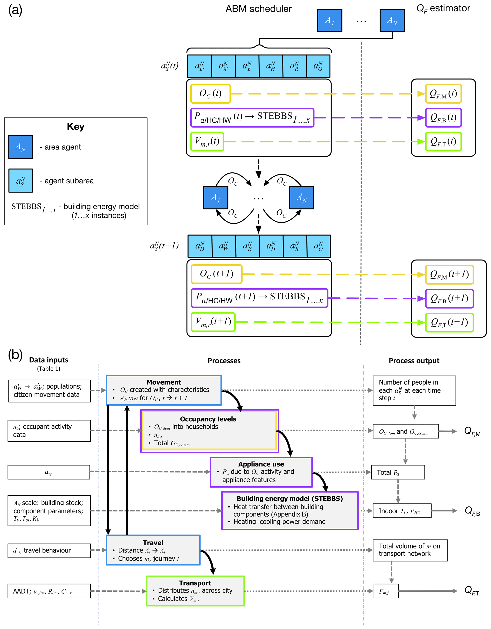
Figure 1Overview of DASH (a) Agent–agent interaction and estimation of QF with the AN (mid blue) to (light blue) relations, changes in process outputs (yellow, purple, green) between time steps and the reaction (arrows) to give QF. (b) Processes include agent–agent interactions (blue boxes), agent reaction and interaction with environment (QF,B: purple; QF,M: yellow; QF,T: green boxes), inputs (dashed lines), process outputs (dotted lines) and their interactions (thick lines), and QF outputs (solid grey lines). Notation list gives definitions.
Given DASH takes an agent-based approach, all processes involve either an interaction or reaction of agents (Macal and North, 2010). The agents represent the decisions for movement and activities of people (e.g. cooking) that impact energy use and therefore QF. The dynamics result from agent activity across multiple processes in each QF source term (Fig. 1a) but share outputs (Fig. 1b). For each spatially scalable agent (Sect. 2.1) there are the following (Fig. 1a):
-
an agent-based model (ABM) scheduler – to capture the evolutionary dynamics (Sect. 2.2) of the spatially discrete agents AN
-
three source-specific QF estimators – they use movement and activity from the ABM scheduler to model metabolic (QF,M, Sect. 2.4.1) and transport-related (QF,T, Sect. 2.4.2) anthropogenic heat; given the dominant role of building energy use to urban anthropogenic heat (Sailor and Lu, 2004; Pigeon et al., 2007; Allen et al., 2011; Sailor, 2011; Nie et al., 2014; Zheng and Weng, 2017; Gabey et al., 2019), a building energy model (Sect. 2.4.3 and Appendix B) is integrated within DASH to estimate QF,B – this accounts for behaviour of occupants that impacts both appliance energy use and any indoor environmental conditioning.
The main DASH workflow is driven by agent–agent interactions with a three-stage process determining QF per time step (Fig. 1b).
-
Stage 1: agent–agent interaction occurs through occupant (OC) exchange processes (blue, Fig. 1b) that are modified by demographics as well as type and time of day.
-
Stage 2: occupancy levels associated with an agent (yellow, Fig. 1b) modify appliance energy use (Pα, Fig. 1), building heating and cooling control (via the building energy model, STEBBS – Simplified Thermal Energy Balance for Building Scheme), and volume of vehicles on the transport network (green, Fig. 1).
-
Stage 3: source-specific QF,B, QF,T, and QF,M terms are calculated for each agent and combined to give QF for each agent's geographical region.
All processes operate at the same spatial unit (rather than area) and time step. These are both defined by the data used to inform the ABM scheduler. Rules that govern the processes may be informed by data and actions at coarser scales.
2.1 Spatial granularity
Agent-based model design allows flexibility as to what “agents” represent; for example, individuals, households, specified areas, or businesses (Crooks and Heppenstall, 2012; O'Sullivan et al., 2012). However, the chosen units should be able to interact with each other and respond. The constraints on selecting the most suitable entity for an agent include the purpose of the simulation, data availability, and computer resources. In DASH, agents represent spatial units that interact by exchange of occupants – the number, activity, and type of which informs the calculations of QF (Fig. 1).
The QF of a spatial unit depends on the number of occupants and their characteristics and activities. For example, in residential areas QF,B increases as occupants wake up and start to use appliances or heating/cooling. As they leave home, QF,T increases as fuel is used for transport and as the OC are passed between agents the changing activity and occupancy numbers impact on each agent's QF. By using spatial units as agents (with OC as an agent property), agents can be scaled according to behavioural data and computational constraints. The relationship of agents to occupants can be from many-to-one and many-to-many. Here, a many-to-many relationship is used, given computational and data constraints.
The agents interact by exchanging OC based on rules associated with the number, type, and activities of occupants. These are also used in calculation of the energy use of an agent, i.e. the agents' response. Agent representation is designed to be data driven (analysed), and so behaviour is constrained by data availability. For individual cities, the context (social, physical) provides the agents probable (exact) characteristics, while administrative boundaries from national census (or other large survey data) will typically constrain DASH.
The agent (AN)-based spatial unit (as determined by data availability) contains subareas () of activity (not spatial units) to which the OC are assigned. Hence, population statistics are needed to characterise subareas. The subarea notation identifies the agent (superscript) and activity area (subscript). In this version of the model, there are six subareas: (i) domestic (), (ii) workplace (), (iii) primary school (), (iv) secondary school (), (v) shop (), and/or (vi) other (). There is a minimum of one subarea in each AN, with the total number and type in each AN to be determined according to available data and city context (e.g. a commercial district may only consist of ). Despite the AN location being static, their properties are dynamic.
As AN have the decision-making capability for exchanging OC, they interact by “releasing” or “accepting” occupants. Spatial variation in OC exchange is provided by the characteristics of the , for example with higher workday populations being more likely to accept occupants during workday hours than other with smaller workday populations. Temporal variability is governed by aspects of human behaviour, with granularity provided by different categories of OC identified within the data used to inform the ABM scheduler. The model can, therefore, capture differences associated with time of day, day of week, type of day (e.g. holiday or not), and time of year within (and across) different OC categories. Thus, this design results in the spatio-temporal dynamics of QF.
Each AN is located within larger spatial units (B) to allow coarser-resolution spatial data to inform model behaviour (e.g. traffic speed limits, school districts), as well as enabling different spatial representation of QF in analysis. Note that there can be multiple levels of directly nested spatial units. This permits different levels of data availability and governance structure (e.g. impacting decision making/options) to be appropriately captured. Hence, impacts from changes in small areas on the surroundings can be explored.
2.2 Rules of AN interaction
OC are generated and assigned to categories used to inform energy demand behaviour and movement (e.g. age, work). To enable movement of OC, they are each associated with subarea types corresponding to different activities. The may be located both within one AN or across as many AN's as there are 's. A minimum of one “anchor” subarea is required per OC to identify a place of residence, . For other activities (e.g. work or formal education) to be captured further 's are needed. Data-driven assignment of occupants to subareas enables the exchange of OC by AN's (Sect. 3.1). The anchor 's are relatively static (i.e. changing infrequently) as for example workplace remains constant for long periods.
If data do not allow direct matching of multiple anchor 's for OC, then is assigned randomly (SciPy, 2019) but in proportion to the available choices. The choice can be informed by rules, such as those imposed by local governing structures (e.g. school choice). For OC trips to non-anchor subareas (e.g. leisure activity, shopping), assignment is stochastic. Gravity weightings (Γ) for all potential trips between origin i and destination j locations (B, for coarser resolution than AN) of distance di,j are precalculated and stored in a matrix (Casey, 1955):
where weights Γi,j are derived by an attractor (e.g. total number of shops) within B and the distance (d) between locations. The destination is randomly selected using gravity weightings (Eq. 3), accepting amenity attraction rules (Reilly, 1953). The process is nested to allow for spatial nesting of agents and account for spatial resolution of data on amenities.
Within an AN, further rules, associated with movement, can be assigned to OC to represent structural and personal factors that impact timing and ability to move between . For example, associated dependants (e.g. children) impact on timing of movement of an OC due to caring responsibilities.
2.3 Evolutionary dynamics
At each time step, the decision for an AN to release OC applies a Markovian approach (Appendix A). This stochastic state determination process decides the nature of an object's (e.g. OC) next state (e.g. ) using knowledge of its previous states (Blitzstein and Hwang, 2019). The subsequent time at which an OC is accepted by the destination AN is influenced by factors such as distance and time of travel. This allows random variability in human behaviour to be simulated such as presence and activities of occupants in a single building (Page et al., 2008; Richardson et al., 2008; Widén et al., 2009a) for long periods (Page et al., 2008), whilst aggregate behaviour (informed social structure) will still be apparent. This requires knowledge (data) based on movement and location associated with time and allows decision making to be identified with individual OC as well as populations.
The movement and location data are used to create the Markov matrices' stationary distributions (Eq. A1) for the exchange of occupants at each time step (t). The Markov matrices are created prior to a model run but could be recalculated between each time step of the model run in order to capture potential response (in movement and activity) to disruptions.
2.4 Calculation of QF
Heat sources (Eq. 2) from people, buildings (with appliance load breakdown), and transport are determined using the OC count and associated activity in each of the 's of all AN's.
2.4.1 Metabolism QF,M
Metabolism (QF,M) of each OC uses an individual metabolic rate (M):
with the sensible (H) and latent (E) components, using the Bowen ratio β (sensible to latent heat) as follows (for one OC):
Both β and M can vary with activity (e.g. office work/sitting, walking, sleeping) and demographics (e.g. age, gender). Occupants are assumed to be indoors when present in an . When occupants travel and are outside, contributions are made to QF,M(T).
2.4.2 Transport QF,T
If an AN releases an OC, the journey time, route and mode of transport are needed to determine QF,T. These allow travel dynamics to influence the time and nature of energy use at the associated spatial unit through a simple traffic model. QF,T is calculated at each time step for the spatial units for each mode type m (e.g. car, truck, train, walk) and route type r (e.g. minor or major road, overground or belowground rail), with speed v (m s−1) and heat emission F (W m−1) for all travelling OC. The journey time is tracked to enable release of OC at appropriate (e.g. timely, delayed) periods at their destination AN by using a mode- and journey-specific time bin (tb). The journey time tb is updated at each time step. The notional duration is found from the mode's distance–time relation using LOWESS analysis (Cleveland, 1988) on travel data for distance travelled.
The total number of travelling OC's in each spatial unit is the sum of OC's in all tb's for all m. The number of OC's in a tb changes at each time step as – and when – new journeys begin. When the tb time is zero, the held OC's are released to the next spatial unit of their journey, which may be a destination or an intermediate location (e.g. mode transfer from walking to bus).
The choice of m is informed by data that associate probability of m to origin–destination pairings. If journey combinations data are unavailable, weighting by distance di,j is used, informed by other sources (e.g. travel surveys). The journey route (through different spatial units that calculate local QF,T) is determined from geographical information system (GIS) data (e.g. OpenStreetMap, 2017), mapping application programming interfaces (APIs, e.g. Google, 2019), or straight-line distances between centroids (in the absence of data). For the latter, spatial nesting can be used between AN and B. Routing options between spatial units can be one (most basic) or many (data dependent).
Route (r) parameters have a capacity limit (Rlim) assigned by r-related spatial (B, AN) capacity constraints (e.g. size and possible number of occupants of a bus or a railway carriage that operate in that area, road congestion limits). However, these may be modified if a disruption impacts part of the transport network (e.g. power failure, intense flooding). The current occupancy is constrained by a mode-appropriate ratio (Cm,r) such as number of occupants () per unit vehicle. For road-related transport, unit vehicle length (Lm) is required as, for example, buses hold more people than a car but require more space on the road. These constraints are informed by local data.
A total vehicle count for each “m, r” (as Vm,r) is used to determine if OC in travel can be moved between spatial units. When both
then Vm,r is incremented by (i.e. ), where . If Rlim (e.g. total road-type length in a spatial unit) is exceeded, OC will not be passed to the next spatial unit – time associated (tb) in neighbouring spatial units will be lengthened. When
then Vm,r becomes .
Where transport is considered at the spatial resolution of B, Vm,r's are distributed to child spatial units based on the ratio of nested spatial unit capacity to the parent spatial unit's capacity (e.g. for cars).
The anthropogenic heat flux from transport, QF,T for an AN of area A, at time t is (Grimmond, 1992)
where Lr,t is the distance travelled in a time step. Heat emission (Fm,f; W m−1) varies with fuel type (f), m, r, and vehicle speed (vm,r; m s−1). For the case of road traffic, speed can be represented as a function of permitted – or average – speed limit (vr,lim). This is linked to traffic density (i.e. vehicles per unit length; e.g. Salter, 1989), which we relate to a ratio of total on-road vehicle length to total route length (equates to Rlim) as
Hence, the speed–density function changes with time as follows (e.g. Greenshields et al., 1935; Wu, 2000):
The relation of vr(t) to Fm,f is dependent on local fuels types (e.g. Grimmond, 1992; Smith et al., 2009) and is part of the model parameters specification (e.g. Sect. 3).
2.4.3 Building energy (QF,B)
QF,B accounts for appliance usage (), lighting (), heating and cooling demands (), and hot water demand ():
These vary by AN as OC composition changes activities , and the local building form, construction (materials and dimensions), and control systems (heating, cooling, lighting) change (e.g. as neighbourhood age or construction period varies). AN release (acceptance) of OC to (from) the movement and travel module leads to a change in occupancy levels in associated building types. Activity of OC informs appliance (α), hot water (HW), and lighting (l) energy use as well as heating and cooling (HC) setpoints for building environmental control.
QF,B is determined through use of STEBBS, which calculates heat transfer through building fabric and ventilation using an adjustable time resolution. QF,M, α, HW, and l provide internal gains to the building volume and fabric (Appendix B). The dynamic 1-D energy model enables both simple representation of individual buildings (Klein et al., 2017), as well as scaling to represent groups of building within an AN. By using building archetypes, STEBBS provides a computationally efficient representation of buildings across a city (Heiple and Sailor, 2008; Bueno et al., 2012; Kikegawa et al., 2014) and permits multiple types within an AN.
For each archetype with an AN, STEBBS requires the building dimensions (width, depth, height), window–wall ratio, and thermo-physical properties for the building components (i.e. window, wall, roof, floor, internal mass). Thermal inertia of appliances and lighting is assumed to be negligible (i.e. no regulating thermal mass), and so the heat resulting from their use (i.e. total power demand Pα) is exchanged directly with the indoor air.
Domestic hot water (DHW; following building services convention this includes both domestic and commercial buildings) heating and air heating–cooling are a response to internal conditions, controlled by a setpoint temperature (Tset; K). The energy use (q) depends on the system efficiency (κ) and maximum power rating (Pmax) for heating using an exponential control to avoid heating overshoot as follows:
And for cooling:
where Ti is the internal water/air temperature (K). Efficiency losses of the heating system and all cooling energy are calculated as direct heat ejection to the outdoor environment. The heating of the building fabric modifies the storage heat flux of the urban energy balance (Grimmond et al., 1991; Grimmond and Oke, 1999). Thus this term is tracked and removed from QF,B. Setpoint temperatures are controlled (between minimum and maximum) in relation to occupancy recognising the one-to-many representation of buildings in the model. Domestic instances vary based on proportion of active occupants to total residential population, whilst non-domestic instances may have setpoint temperatures based on occupancy thresholds.
Ventilation loss/gain (qvent) is given as (Spitler, 2011)
where VR is the ventilation rate (m3 s−1), ρa is the air density (kg m−3), cp is the specific heat capacity of air at constant pressure (J kg−1 K−1), and To is the outdoor air temperature (K). In the stand-alone version of this model no spatial variations in these are considered. If coupled to a meteorological model, these outdoor variables can be spatially dynamic and respond to QF emissions locally (Sun and Grimmond, 2019).
DHW is considered as a sensible heat gain only (no latent), with hot water to drains unaccounted for in QF,B. Heat exchange between DHW in storage (tank and water pipes) and building volume is accounted for. Volumetric flow rates (VFR, m3 s−1) of DHW use and to drain can be set to control volume of DHW in use. The internal heat gain from this varies with OC level and activity.
The combined internal gains based on internal building activities are passed to STEBBS. The number of active (i.e. present and awake) OC's in a building (e.g. domestic, work) influences total energy use (Druckman and Jackson, 2008; Yohanis et al., 2008) and the energy demand profiles at timescales from seconds (Richardson et al., 2010) to hours (Widén et al., 2009b). Hence, occupancy levels are essential to reproducing commercial (Kim and Srebric, 2017) and domestic load patterns (Widén and Wäckelgård, 2010).
Hence, each building archetype within an AN is impacted by its OC level and their activities (i.e. ). As OC categories (e.g. age related) participate in different activities (e.g. infant differs from adult), local census (or other) data both constrain and spatially inform OC characteristics.
Lighting and appliance gains are associated with activity, appliance type α (Firth et al., 2008) set efficiency, and power usage (Pα) associated with different building types (e.g. commercial, domestic). We distinguish three energy consumption classes:
- i.
active only (AO) – only occurs with user activity (e.g. oven, iron);
- ii.
continuous (C) – always consuming energy (e.g. cold appliances: fridge, freezer; small appliances: telephone, clock, burglar alarm); as these may cycle power (e.g. cold appliances) the power rating accounts for the fraction of time the appliance draws power during a single complete cycle and the mean power consumed whilst operating;
- iii.
active/standby (AS) – two modes which depend on user activities (e.g. television, computer): (1) as AO and (2) less when not actively used.
Each appliance (α) type (j) is assigned to AO, C, or AS with an active power rating αp and additionally for AS appliances a standby rating αs. The number of appliances of type j in AN () is determined by domestic/non-domestic appliance market permeation (αj,k) as
where nb is the number of households (domestic), number of work desks (non-domestic, commercial), or floor area (non-domestic, other) in an AN; acts as the limit of appliance use at any time. If no distinction between j use profiles can be given (data dependent), all appliance demand is combined as one type.
For domestic use, households are categorised by total number of residents such that proportion of (by AO, C, or AS) in use at a given time t is
with the fraction of households with x active occupants using αj at t (based on occupant activity scheduling) and nb,x(t) the number of households with x active occupants at t. For non-domestic buildings, appliance use is proportional to occupancy level and lighting is considered part of this load.
The power demand Pα (W) of all appliances in use is
and is the heat gain passed to each STEBBS instance (i.e. each building archetype per AN). Appliance characteristics are currently uniform throughout AN but could be variable (e.g. by socio-economic structure).
Domestic lighting is considered as a separate load impacted by an outdoor downwelling shortwave radiation threshold (K↓lim), a number of households with active (awake) occupants nb,x, and a base/min/max luminous intensity, , per household for scaling lighting requirement (Widén et al., 2009a):
Luminous intensity is converted to total power (Plight) using a per light power rating (Pl). This is passed to STEBBS as part of the appliance load Pα.
3.1 DASH setup and data sources
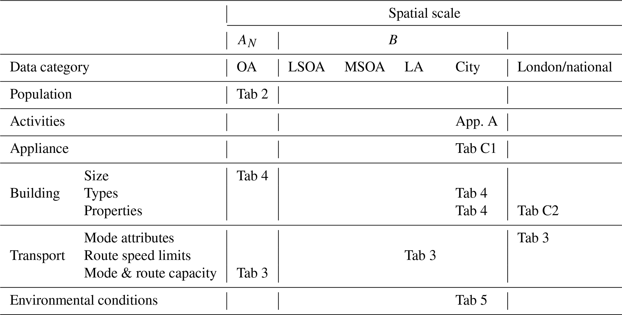
We evaluate DASH in Greater London (GL). In the United Kingdom (UK), the output area (OA) is the smallest spatial unit for census data. We adopt the OA as the agent spatial unit (i.e. AN) in the model runs, with AN nested within four coarser spatial units (B): lower-layer super output area (LSOA), middle layer super output area (MSOA), local authority (LA), and city/region as data (from various agencies) are aligned to one or more of these spatial units. The LA have several governance roles (traffic speed, school districts, planning decisions, etc.) that will impact energy use (LGA, 2019). Similar structures are used in other countries but with varying levels creating the complete city (National Bureau of Statistics of China, 2017; Statistics Bureau of Japan, 2017; Statistics Canada, 2017; US Census Bureau, 2019). In London there are 25 053 OA (determined by residential population and social homogeneity; ONS, 2017a) that vary in size from to 12.3 km2, 4835 LSOA, 983 MSOA, and 33 LA within one Greater London Authority region (Table 1).
Table 1Sources of data used by DASH and the highest spatial resolution (columns) used in Greater London. Details are given in the other tables (Tab) and appendices (App.) indicated. Notation defined in text.
The UK Time Use Survey (TUS) 2014–2015 (Gershuny and Sullivan, 2017) provides a structured source of data for simulating population movement and human activity (Iamarino et al., 2012; McKenna et al., 2015; Baetens and Saelens, 2016). Such surveys are carried out in many countries by governments or research institutes (Fisher and Gershuny, 2013), allowing DASH to be applied elsewhere with appropriate cultural practises accounted for. In the UK TUS, residents record their activities and location for 1 weekday and 1 weekend day, normally creating profiles of individuals with income, age, sex and household type metadata. The data samples are sufficient to allow analysis at national to regional (e.g. GL) scale in many cases. The 10 min time step resolution of TUS data (Gershuny and Sullivan, 2017) is the basis for the model time step.
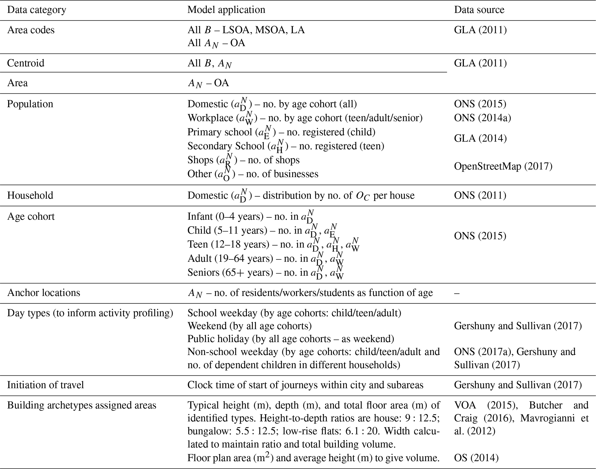
The TUS data are used to construct Markov chains (Appendix A) that govern the exchange of occupants in DASH (Fig. 1a) and the levels and type of activities undertaken by different groups of OC across the day (Sect. 2.3, Table 2). Age cohorts (Table 2) are used as the group identifier. Appliances attributed to TUS activities (Table 2) have different power ratings and market permeation (Tables 3, C1). Non-domestic activity varies by workplace appliance types according to the land use (e.g. industrial, office) of the AN (BEIS, 2017a; OpenStreetMap, 2017) with appliances (Table D1.iii) having greater energy consumption in industrial than commercial areas.
Table 2Spatial, temporal, and demographic data used to inform activity in Greater London. Data sources: Greater London Authority (GLA), Office for National Statistics (ONS), Chartered Institution of Building Service Engineers (CIBSE), Ordnance Survey (OS), Valuation Office Agency (VOA). See also Table D1.
The application is undertaken for 2015 to coincide with the TUS data, when GL had a population of 8.539 million (census data updated annually; Table 2). The remaining data needed are obtained for the closest year. Throughout we endeavour to use open-source, freely available data. A variety of data types are used, at a range of spatial resolutions (Table 1) with more detail given subsequently (Tables 2–5).
Movement of occupants is informed by the National Travel Survey (DfT, 2017) and census data on commute patterns (§8,10, Table 4), to determine choice of mode by distance or type of journey providing the travel attributes (Table 4). In this evaluation, nine modes of transport (m) exist: cars, motorcycles, vans, taxis, buses, surface rail, underground rail, cycling, and walking. Other deployments could include freight- and boat-related modes. Exclusion of freight vehicles does not directly affect the travel dynamics but will result in an underestimation of QF,T. Route types (r) considered, include four road types – residential, minor (so called B roads in the UK), major (UK's A roads), and motorways (highways) – and two rail types (underground and surface). In the model runs, journey distances for all routes that move between LAs are determined at LA scale based on GIS shapefile LA centroids. This is the coarsest implementation of the transport component of the model.
Table 3Data sources for physical building characteristics applied to building archetypes. Symbols in notation table. Symbols used are L: wall thickness (m); ρ: building material density (kg m−3); ke: wall effective thermal conductivity (W m−1 K−1); ε: emissivity; h: convection coefficient (W m−2 K−1); VT: volume of tank (m3; dependent on number of persons per household); and ToU: time of use. Data sources: §1 – British Council for Offices (BCO, 2009), §2 – Richardson et al. (2010), §3 – DECC and BRE (2016), §4 – Hawkins (2011), §5 – DECC (2015), §6 – HCA (2010), §7 – Butcher (2004). §2 is used for cycling patterns of continuously on appliances (i.e. fridge/freezer). See also Table D1.
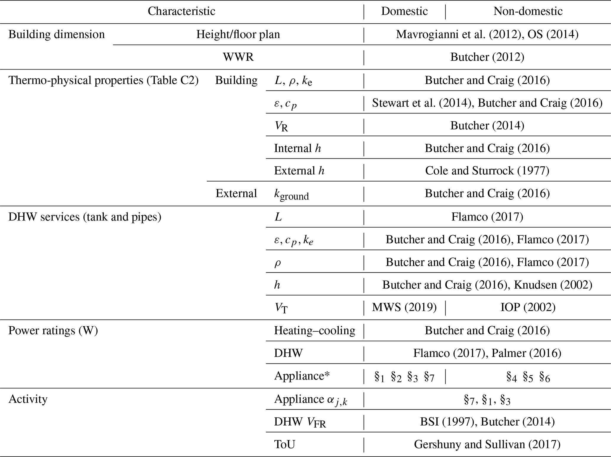
* see further details in Table C1
STEBBS is used with different parameters for domestic and non-domestic buildings (Field, 2008). We simplify to the three most common domestic building (houses, bungalows, and flats) archetypes in GL, varied by presence at LSOA level (Table 3; Mavrogianni et al., 2012; VOA, 2015). Despite advances in non-domestic building characterisation for GL (Evans et al., 2019), the heterogeneity in form and use limits the use of a range of archetypes (Steadman et al., 2000). Again, for simplicity in this evaluation, we use a single STEBBS characterisation based on the most common domestic archetype parameters for non-domestic (e.g. shops, hospitals, offices). Hence, a maximum of four STEBBS instances per AN with the appropriate building fabric thermo-physical properties assigned from one of two building age groups (pre- or post-1965; Tables 3 and C2). Building dimensions are informed by total AN building footprint and height (Table 3) for each archetype by age category. The limited consideration of building material thermo-physical properties and dimensions is expected to reduce the spatial variance in heating and cooling contributions to QF in DASH. DASH can use more building features given suitable input data.
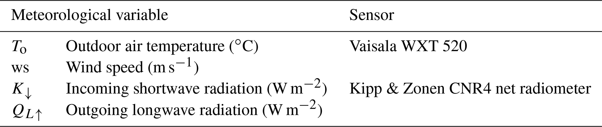
Meteorological data to force the model are from the KSSW site in central London (Kotthaus and Grimmond, 2014, Table 5). Means (1 and 5 min) are used to obtain 10 min means (model time step). Outgoing longwave radiation observed with a Kipp and Zonen CNR4 radiometer (Table 5) is used assuming an emissivity of 0.9 (Butcher and Craig, 2016) and Stefan–Boltzmann equation (Oke, 1988) to obtain surface temperature. Soil temperature (at 5 m depth) is assigned assuming it is equivalent to the mean annual (2014–2015) air temperature (Sellers, 1972; Busby, 2015) of 11.9 ∘C.
Table 4Data sources for (a) modes and (b) routes. Variations from data include the following: buses: 85 % diesel of fleet (in 2015) and rest mostly hybrid; electric (EV) and low-emission vehicles: EV cars 0.2 % of GL registered vehicles (2015) (DfT and DVLA, 2019). Data sources: §8 – ONS (2014b); §9 – ONS (2018); §10 – DfT (2017); §11 – DfT (2014a, b); §12 – London Datastore (2014); §13 – OS (2016); §14 – Smith et al. (2009); §15 – Highways Agency (2017); §16 – TfL (2018); §17 – TfL (2019); §18 – OS (2015); §19 – TfL Train and Underground Rolling Stock Information Sheets from §10; §20 – TfL working timetables from §10; §21 – Iamarino et al. (2012).
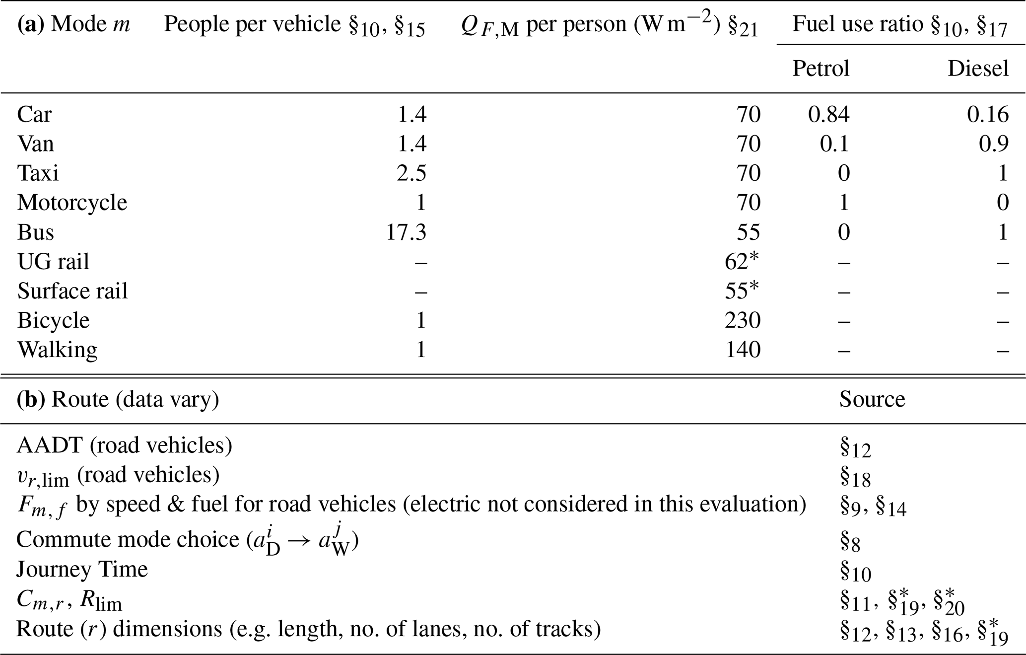
∗ Not applied in evaluation.
Table 5Observed meteorological variables at King's College London KSSW site, 60.9 m above ground level (Kotthaus and Grimmond, 2014; Ward et al., 2016). See Fig. 1a in Kotthaus and Grimmond (2014) for site location. From these other variables are derived.
As the model requires continuous atmospheric data, gaps are filled in consecutive order: (a) linear interpolation when less than 4 h; (b) median for same time in the surrounding ±48 h for gaps of 4–24 h; and (c) similarly for gaps greater than 24 h, using the median ±72 h. The various model runs (Table 6) have a spin-up period of 24 h (144 time steps) for the STEBBS model to become stable.
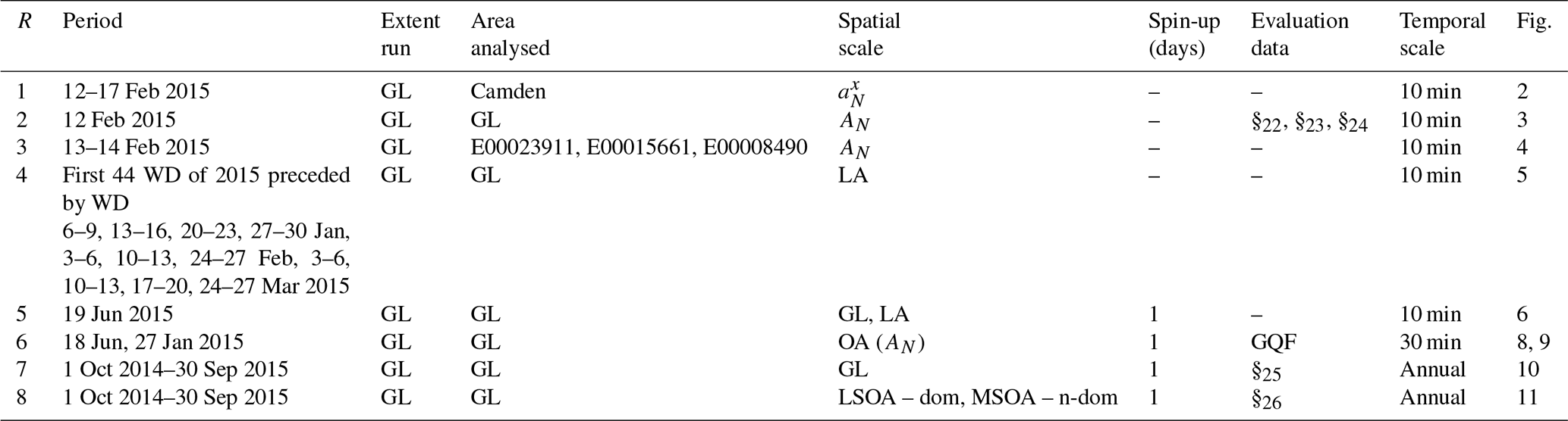
Table 6DASH model runs (R) setup. Runs are characterised by period (dates and day types; WD: weekdays), areal extent (Table 1, dom: domestic; n-dom: non-domestic). Data sources: §22 GLA (2014), §23 ONS (2015), §24 ONS (2014a), §25 National Grid (NG, 2015), §26 BEIS (2017c). Other details are given in Appendix D and Sect. 2. All data have been archived at https://doi.org/10.5281/zenodo.3745523 (Capel-Timms et al., 2020).
3.2 Evaluation methodology
Ideally a model is evaluated with observations of the simulated variables (Table 6). However, direct observations of QF are extremely limited or are indirect with a series of assumptions within them. At the neighbourhood scale, combining radiation and eddy covariance observations while assuming energy balance closure has been used to assess monthly and daily values (e.g. Offerle et al., 2005; Pigeon et al., 2007). Using satellite earth observation, a much larger spatial extent (e.g. city wide) is observed but with a bias to clear-sky conditions. The snapshot values at the time of the satellite overpass require a very large number of assumptions in addition to energy balance closure (e.g. Chrysoulakis et al., 2018). The closest to “direct” measurements of QF are microscale emissions from building vents (i.e. part of QF,B) using eddy covariance sensors (Kotthaus and Grimmond, 2012), but there are extremely limited data available. Thus, the spatial and temporal scales that DASH is capable of simulating cannot be directly compared to measured QF. We therefore use a series of different sources of public data and another model to evaluate various aspects of DASH.
The reference model used, GQF (Iamarino et al., 2012; Gabey et al., 2019), is a top-down inventory QF model developed for London. This is selected as it is amongst the most (spatially and temporally) detailed models for London currently available (Gabey et al., 2019). We apply it to 2014–2015 to align with metered data used in the evaluation. The model uses energy consumption, traffic, and workday population data to provide half-hourly estimates of QF at city, LA, and OA resolutions. Hence, QF estimates for both models are at city scale with OA resolution.
There are several GQF features that restrict DASH being evaluated in higher detail. These are as follows: (i) GQF uses data from a range of scales (up to national) to determine OA results with population weighted disaggregation; (ii) diurnal patterns are prescribed based on either assumptions or coarse spatial data, with variation by day type (weekday, weekend) and season – meaning variability at smaller scales are not captured; (iii) GQF assumes the same diurnal profile for both gas and electricity usage; and (iv) effects of temperature in GQF are the net seasonal diurnal energy use profiles rather than reproducing the day-to-day conditions in London. Hence, individual DASH diurnal patterns cannot be evaluated against GQF with fine temporal or spatial resolution as differences are expected.
To evaluate DASH, appliance (including cooking) power demand is equated to GQF electricity demand and DASH heating and cooling demand to GQF gas demand. This will lead to discrepancies as the demand profiles used in GQF are not energy carrier or vector specific. The calculation and evaluation of QF,T is undertaken at AN scale rather than individual routes. In both models, many of the minor residential roads in AN are unaccounted for.
DASH evaluations (Table 6) use annual (1 October 2014 to 30 September 2015) publicly available gas and electricity consumption data (GW h) for domestic and non-domestic (commercial and industrial) use (BEIS, 2017a, b) and national gas transmission operational data for the same period (NG, 2015). DASH, run with the appropriate meteorology (Table 5), OA results are aggregated for assessment to the LSOA (domestic) and MSOA (non-domestic) scales. These evaluation data have some issues: (i) some non-domestic meter data are undisclosed at MSOA level but appear at LA level (without a MSOA) (BEIS, 2018); (ii) meters with insufficient address metadata cause underreported consumption statistics for some areas; (iii) some gas consumption statistics may be wrongly classified (domestic/non-domestic) as this is done based on annual consumption (threshold =73 200 kW h yr−1) (BEIS, 2018); and (iv) spatial misallocation of metered commercial gas consumption to the billing address rather than actual building/location of use (BEIS, 2018).
Basic metrics assessed include the median (50 %), interquartile range (IQR), and standard deviation (SD). To evaluate the modelled (XM,i) and observed (or reference) (XO,i) time and/or spatial data series both the difference,
and the absolute errors,
are determined, from the following:
-
Cumulative distribution of AEi (obtained from all values, e.g. across all 25 053 OA; Fig. 9).
-
Maximum-normalised value: nMax (e.g. Fig. 10).
-
Normalised errors (%): nE (e.g. Fig. 11a, b,; ideal value would be 0).
-
Absolute normalised error:
AnE (e.g. Fig. 11c, d; ideal value would be 0).
As behaviour, demographics, and travel choices influence the temporal and spatial variation in movement and activity profiles in DASH QF estimates, we examine these first. A critical control on QF is the number of occupants within an area. The area itself may be static (e.g. where buildings are located) or moving (e.g. transport area). The occupancy level will change as people travel to different locations (Fig. 2).
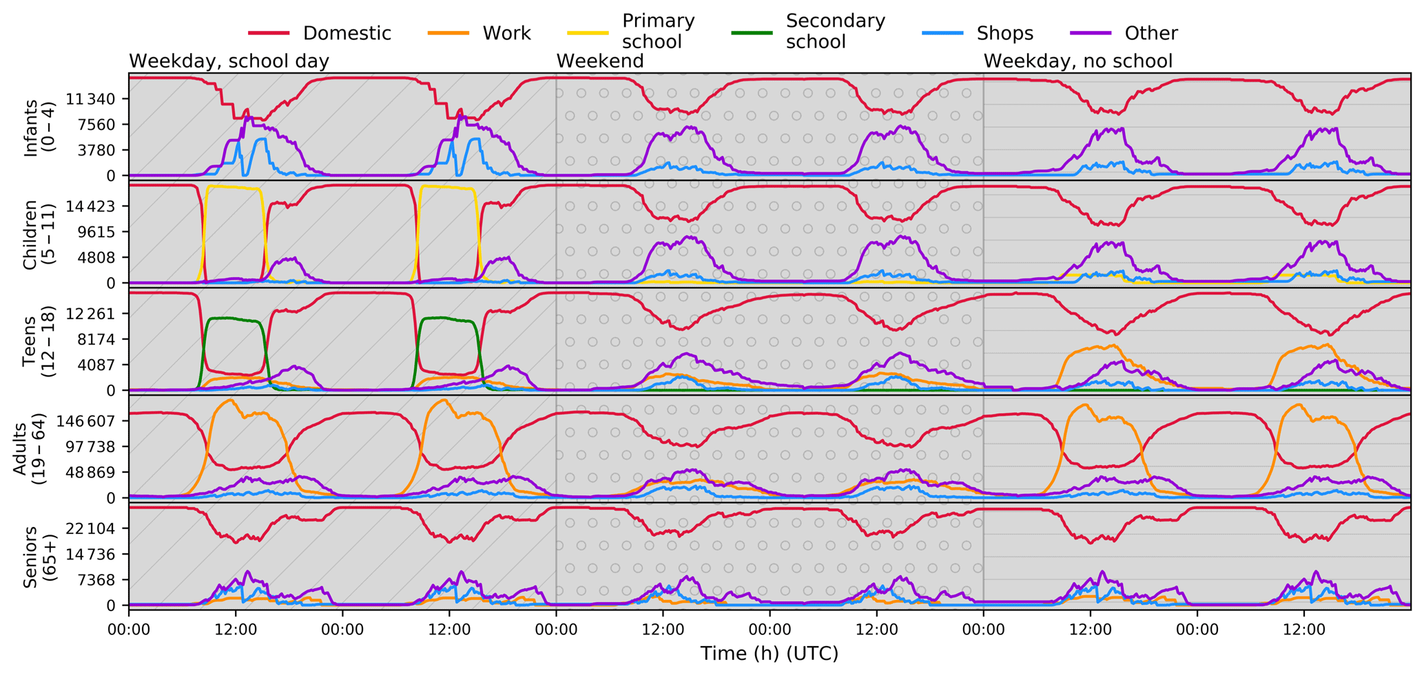
Figure 2Total occupancy of each in one LA for five age groups across 6 consecutive days of three types (textured background): SW (diagonal lines), WE (dotted), NS (horizontal lines) (R1, Table 6).
In model run R1 (Table 6), the results for one B spatial unit (LA Camden, London) are used to demonstrate the OC movement and travel through time (6 consecutive days) within each for each age group for three day types (weekday – school/non-school, weekend) as a result of AN occupant exchange (Sect. 2.2). The occupancy levels vary by day type and between age groups, whilst having general consistency within day type by age cohort. Note, people travel outside (and into) this B during the period, but no perturbation is undertaken (e.g. changing transport availability or road construction).
During school weekdays most children and teenagers are in school (, ). Adults, some teenagers, and some seniors work during all day types and during all times of day. Adult occupancy at work (increase at home) is slightly lower on non-school (NS) weekdays than school/work (SW) days as a result of childcare – a small dip observed during noon on NS and SW days that reflects lunchtime activity. , , and occupancy levels increase after peak school and work times, with occupancy returning to similar levels each night.
The occupancy levels of each , , , and are partly informed by population data, so it is important that realistic values occur from the movement processes. This is assessed by comparison of the median and IQR of the total occupancy across each in the city to the static populations of each AN and subarea (i.e. residential, workday, school populations) for 1 weekday (Fig. 3). Hence, a value of 1 indicates the total population is present. occupancy levels have a median peak just over 0.6 of the workday population. AN interaction in DASH allows for different types of work, such as full/part-time and shift work, as it is inherent to the movement data (in this case the TUS; Table 2). Whilst this might not reflect the accurate behaviour of a particular (e.g. an comprising entirely office work may in reality only be occupied 09:00–17:00 local time), the total variability over a group of may be more realistic, given varying work times between commercial sectors.
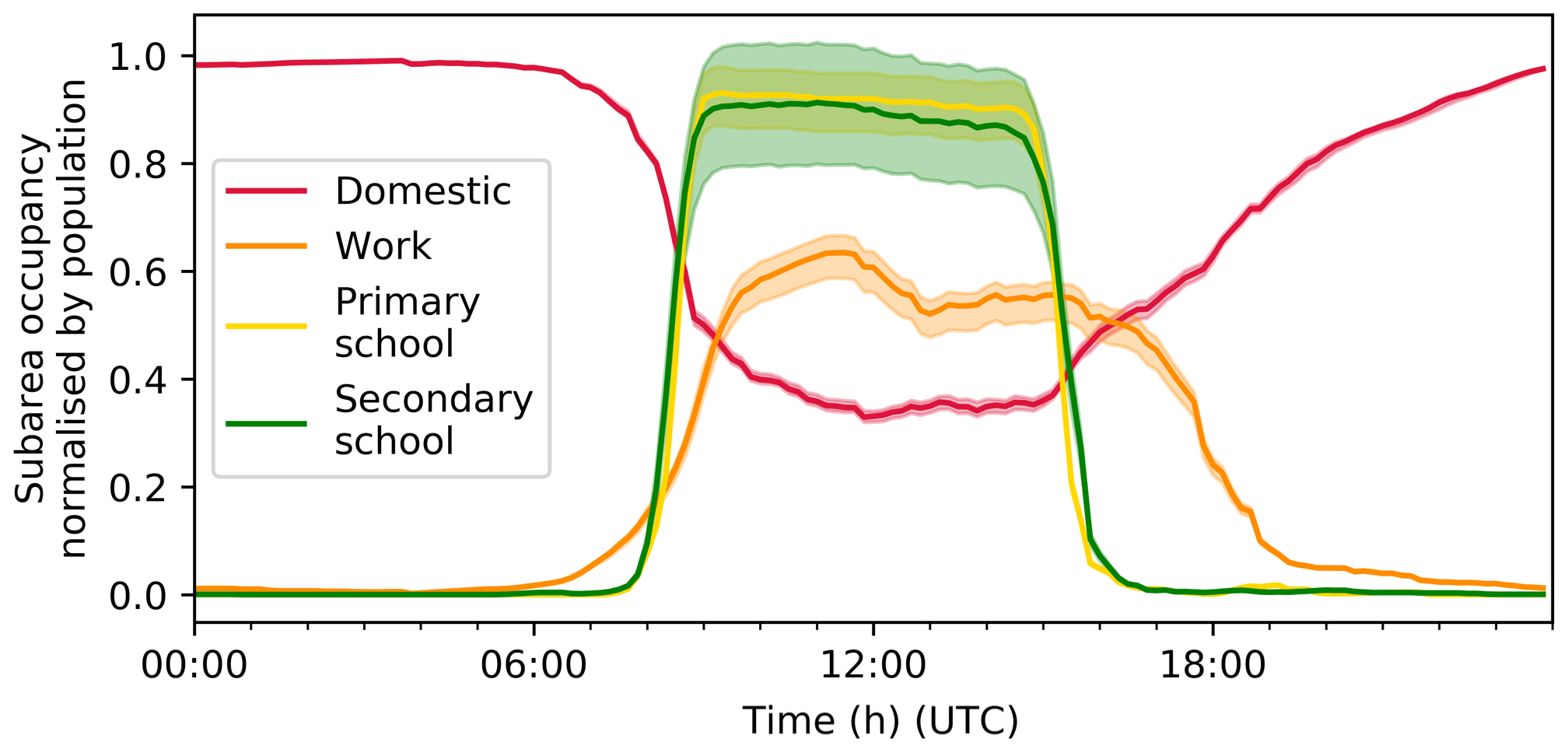
Figure 3Median (line) and IQR (shading) of total occupancy of each in Greater London for 1 weekday (R2, Table 6), normalised by actual static population (Table 2).
For R2 (Table 6) both and IQR occupancy levels are less than some AN school populations (Fig. 3), but for morning to noon the population is exceeded in some areas. Both the deficit and surplus may relate to the method of assigning school anchors to child and teenager OC (Sect. 2.2). If the age group residential population is lower (higher) than the school population in a LA, there will be too few (many) students occupying this LA schools during the day. As students are assumed not to cross LA boundaries, given state school catchment area restrictions. In Greater London 89 % of pupils are in state schools (DfE, 2019).
The occupancy levels are always below 1. The highest values occur overnight when most people are expected to be at home. The narrow IQR indicates there is little variation in total occupancy levels between areas. Variations are expected with active occupancy (e.g. household sizes; Sect. 2.3.1) and in with large differences in resident age groups.
Total occupancy varies with behaviour of different age groups and will affect the power demand within the neighbourhood. To demonstrate the impact of demographics on daily profiles of OC in the , three AN's (neighbourhood, OA, scale) with similar residential populations but different dominant age cohort are compared in Fig. 4 (R3, Table 6). The of each of the three AN's have distinct dominant age groups as follows: , 78 % (291) of residents are seniors; , 92 % (297) of residents are adults; and , 47 % (300) of residents are infants, children or teenagers. In (Fig. 4a), daytime OC remains proportionally higher (Fig. 4d) than (Fig. 4b) and (Fig. 4c). has a steeper morning decrease in OC and earlier inflection point in the afternoon than , likely due to formal school day lengths (Fig. 2). On the weekend day, all age groups, apart from teenagers, follow similar patterns, with about 60 %–70 % remaining in the AN (Fig. 4d).
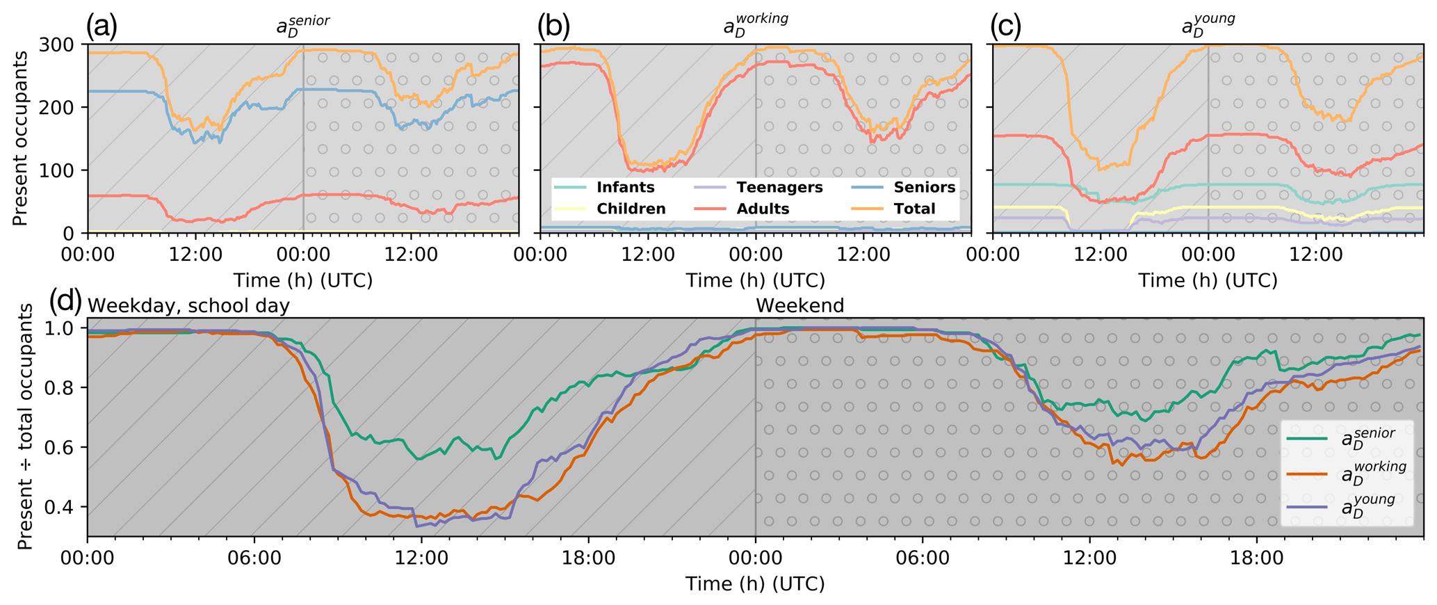
Figure 4Present occupancy levels (R3, Table 6) in three 's by day type (textured background): (a) (number of people per age group living in the area: 0 infants, 2 children, 0 teenagers, 61 adults, 228 seniors); (b) (5 infants, 6 children, 3 teenagers, 274 adults, 9 seniors); (c) (77 infants, 41 children, 24 teenagers, 157 adults, 1 senior). (d) Normalised total occupancy levels for the three 's.
The diurnal pattern of occupancy levels by day type is consistent between days and boroughs (R4, Table 6). The variability in borough occupancy levels for (Fig. 5a) and (Fig. 5b) is greater in the daytime when movement is more likely. Although, these standard deviations are quite small compared to the actual LA-level residential (8760–379 691 residents) and workday (58 444–356 706 workers) populations (ONS, 2014a, 2015). This demonstrates that the occupancy exchange method (Sect. 2.2) produces variation in occupancy levels on a daily basis when the same parameters are used for each day.
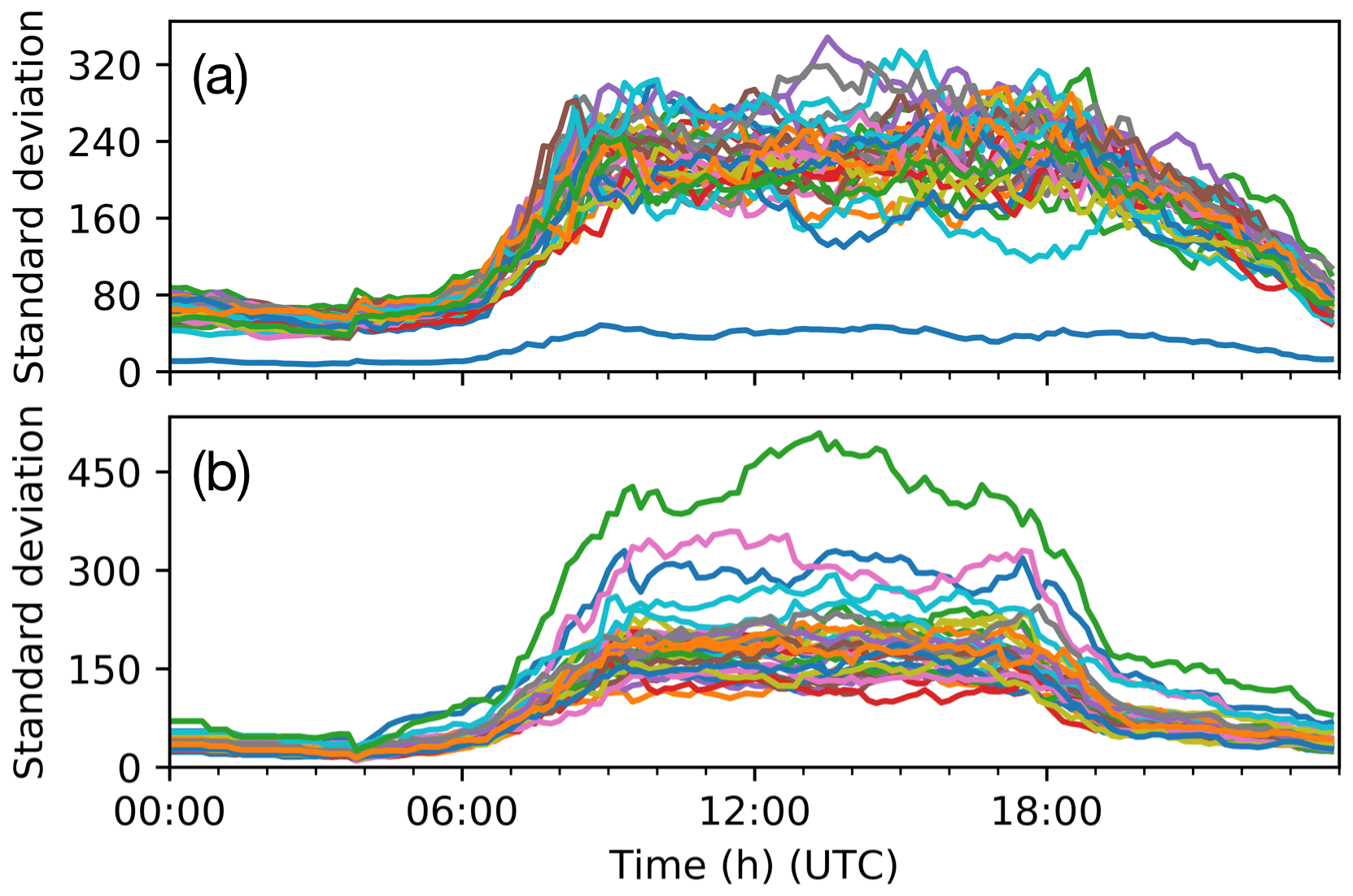
Figure 5Standard deviation of LA (all boroughs of London, colours; for 44 weekdays preceded by weekdays) active occupancy levels (R4, Table 6) for (a) and (b) .
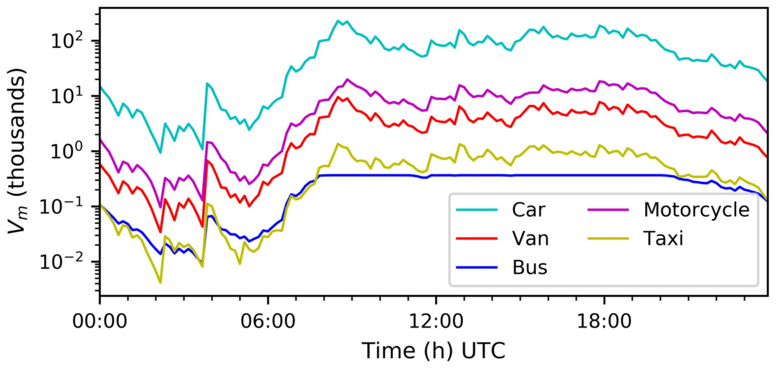
In this road vehicle evaluation (R5, Table 6), routing is at LA scale with inter-LA routes determined using Google Directions (Google, 2019). The volumes of vehicles in use by mode (Fig. 6) predicted by the movement component (Fig. 1, Sect. 2.3) peaks in the morning (07:30–09:30 local time). Slight increases are present around noon and early evening. Low values (00:00–06:00 local time) occur when movement is low (Fig. 2). The increase at 04:00 local time is due to both low sampling and the temporal boundary of the TUS, which considers a day's worth of entries to occur 04:00–04:00 local time. The volume of buses is constant over the period 08:00–20:00 local time due to an imposed condition on capacity that represents an increase in Cbus,r (Sect. 2.4.2) instead of increasing Vbus,r. With only one route option given per LA origin–destination pair, road traffic is distributed between AN in proportion to LA total road area. Routing options at AN scale have not been implemented.
The evaluation of DASH assumes average or typical conditions (i.e. no disruptions are imposed to modify movement and/or timing of activity). As a result, the contribution of appliance use to QF,B is expected to be similar for all days of each type (e.g. weekday, weekend) throughout the year for both domestic and commercial settings (seasonality in appliance-based activity is not considered). In a non-perturbed state, variation within day types across a year is expected to come from heating (space and water) and cooling use as these demands respond to immediate environmental forcing within DASH. As GQF (Sect. 3.2) only varies electricity demand with day type and season, and gas varies with season, we compare the DASH diurnal pattern and magnitude of QF,B components for two school weekdays (SW) in different seasons (summer: 18 June 2015; winter: 27 January 2015). The mean air temperature is warmer in summer (17.0 ∘C) than winter (7.0 ∘C) and has more total radiation (Fig. 7).
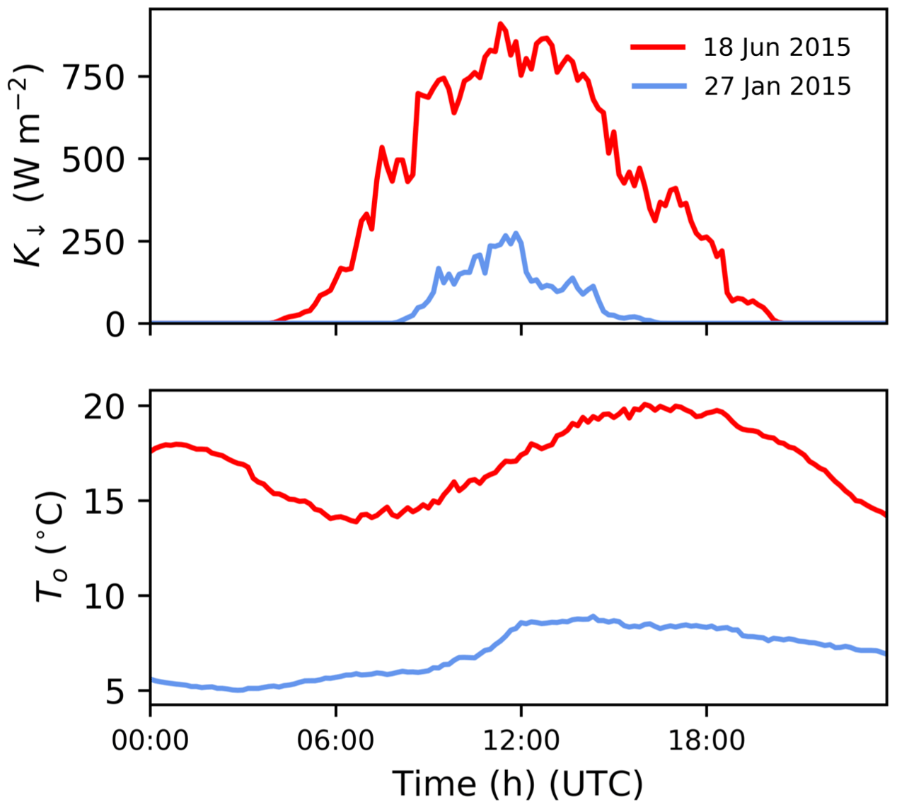
Figure 7Incoming shortwave radiation (K↓; W m−2) and outdoor air temperature (To; ∘C) for 2 SW days. Observations (Table 5) are assumed to be constant across the domain in all runs (Table 6).
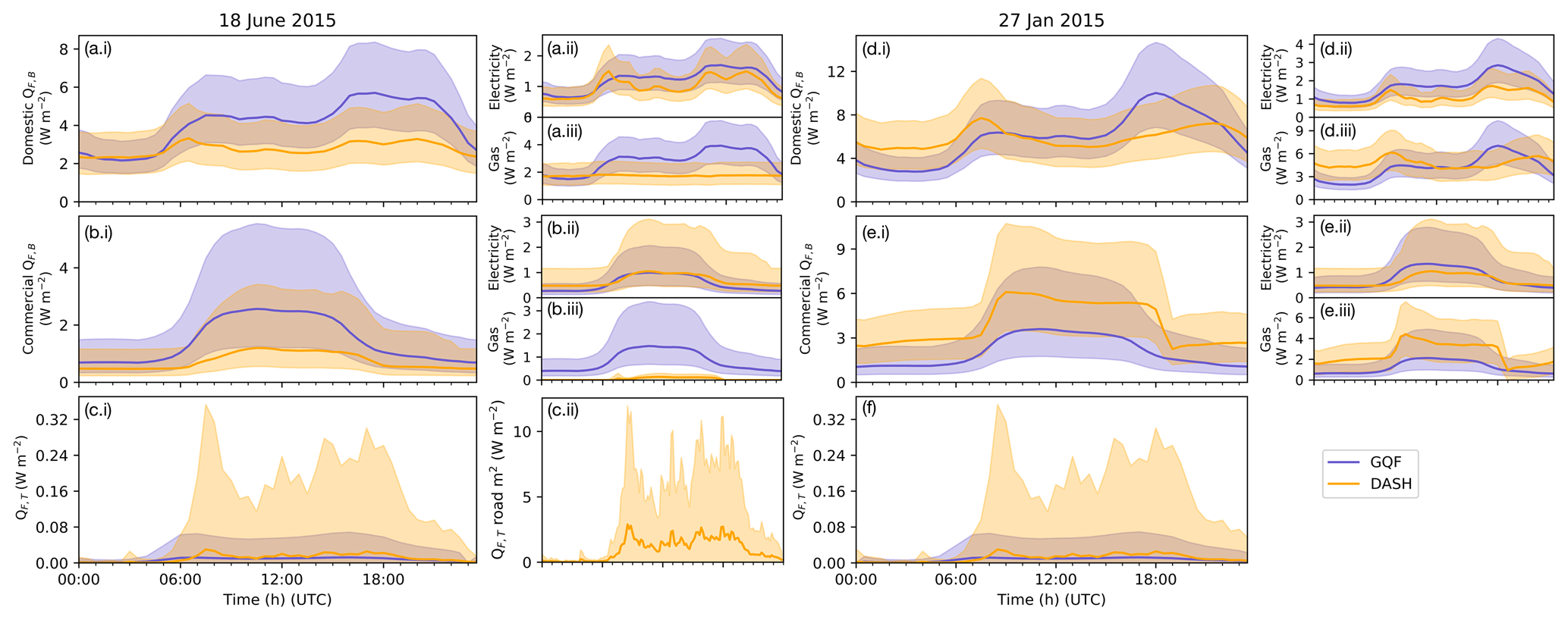
Figure 8Analysis of QF (R6, Table 6) median (line) and IQR (shading) in 2015 for (a, b, c) 18 June and (d, e, f) 27 January – showing total QF,B for (a.i, d.i) domestic and (b.i, e.i) commercial, with the following: (a.ii, d.ii) domestic electricity (GQF) or appliance power demand (DASH); (a.iii, d.iii) domestic gas (GQF) or heating + cooling + hot water demand (DASH); (b.ii, e.ii) commercial electricity (GQF) or appliance power demand (DASH); (b.iii, e.iii) commercial gas (GQF) or heating + cooling + hot water demand (DASH); and (c.i, f) QF,T at AN scale and (c.ii) QF,T for road area only. Figure 7 shows weather conditions. Figure 9 shows absolute errors between the two models.
To evaluate heat emissions from buildings (QF,B), the city-wide emissions of domestic (dom) and commercial/non-domestic buildings (n-dom) are considered separately (R6, Table 6). As DASH and GQF have the same spatial resolution, comparison is made between spatial interquartile ranges (IQR) at the GQF 30 min temporal resolution (i.e. 30 min means – time ending – are calculated from the DASH 10 min values). DASH appliance emissions () are compared to GQF electricity demand (), whilst combined heating (space and water) and cooling in DASH are equated to GQF gas demand ). Discrepancies between values are expected – for example in some areas heating may be powered by electricity.
For the summer weekday, DASH domestic QF,B has similar characteristics to GQF with consistent morning and evening peaks. The mean and IQR are similar from midnight to 05:00 local time but consistently lower (difference in medians of 2–2.5 W m−2) in DASH from the morning to end of evening peak (Fig. 8a.i). Across spatial AN's, more than 60 % have an absolute error (AE; Eq. 20b) of ≤2 W m−2 for all times sampled, and for ∼90 % the AE ≤5 W m−2 (Fig. 9a).
Domestic closely follows in both pattern and magnitude on the summer day. DASH has three distinct appliance demand peaks: morning, midday, and evening (larger, more sustained peak). The magnitude and timing of and peaks are similar between DASH and GQF, although the morning peak in GQF is maintained with less variability throughout the day (Fig. 8a.ii). The domestic summer day gas (GQF) and heating–cooling (DASH) QF,B profiles (Fig. 8a.iii) have the largest discrepancy in daily profile and magnitude. Under summer conditions, DASH heating–cooling is largely driven by hot water demand as indoor temperatures in all instances of STEBBS are passively maintained between heating and cooling setpoints.
DASH domestic QF,B has a more distinct morning peak in winter (Fig. 8d.i), and from midnight to the morning peak DASH values are 1–4 W m−2 greater than GQF. This is caused by greater and may relate to greater sensitivity to temperature for DASH and low outdoor air temperatures. The evening peak is less pronounced and shifted to later evening, with roughly 70 % of the AN having AE ≤5 W m−2 at 18:00 local time (Fig. 9b). All other times analysed were more in agreement with GQF. remains similar to the summer values (Fig. 8a.ii) as the only seasonal variation is due to indoor lighting. After the morning peak it is slightly lower than (Fig. 8d.ii) but follows a similar pattern throughout the day. This discrepancy is likely due to electric heating use, which would include on both a small (e.g. space heaters) and large (e.g. “district” electric heating in high-rise flats) scale.

Figure 9Ranked cumulative frequency of spatial AEi (Eq. 20b) with 2 and 5 W m−2 (vertical lines) and maximum (key; W m−2) indicated at six times (colour) for R6 (Table 6, Fig. 8) in 2015 on (a, c, e) 18 June 2015, (b, d, f) 27 January 2015, for (a, b) total domestic QF,B (c, d) total commercial QF,B, and (e, f) total transport QF,T. Note y axes are different between rows (50 % of spatial units shown by horizontal dashed line if applicable) and x axes are log10.
Summer commercial QF,B is consistently lower in DASH (median ∼1.5 W m−2 less) than GQF in the middle of the day (Fig. 8b.i), with morning and evening medians more similar. The evening IQR increases for DASH and is reflected in , likely associated with energy demand from commercial properties that remain open later in the evening (e.g. leisure facilities). There is close agreement between and medians (Fig. 8b.ii). At least 60 % of AN agree within 2 W m−2 for all sampled time steps (Fig. 9c).
The winter diurnal patterns for commercial QF,B are similar for DASH and GQF (Fig. 8e.i), but DASH has a steeper morning (evening) increase (decrease) as well as consistently higher values (median 2–3 W m−2 in the daytime). The evening decrease starts ∼2 h later in DASH. These higher values are due to (Fig. 8e.iii), which dominates the total pattern. The median and profiles (Fig. 8e.ii) are in good agreement, with slightly broader IQR for DASH. More than 50 % of AN's have a MAE of ≤2 W m−2 for all times except 09:00 local time, which is slightly below 50 % (Fig. 9d).
For both domestic and commercial use, summer 's have the largest discrepancy in profile and magnitude compared to (Fig. 8a.iii, b.iii). In summer for DASH, is expected to dominate as indoor temperatures in all instances of STEBBS are passively maintained between heating and cooling setpoints. City-wide domestic QF,B is greater than commercial QF,B in both DASH and GQF.

Figure 10Daily (1 October 2014–30 September 2015) DASH normalised total HC and DHW energy demand (R7, Table 6) for Greater London, minimum and maximum London outdoor air temperature (∘C) (Table 5), and normalised national gas demand (NG, 2015). See Sect. 3.2 for normalisation.
The median QF,T values are fairly similar between both models, but GQF has less temporal variability (Fig. 8c.i, f) with IQR. As DASH responds to variations in travel demand and exchanges occupants across the city more temporal variation occur between AN. Figure 9e and f, show small MAEs between the two models, with more than 98.5 % of AN within 2 W m−2. When considered for road area only, DASH QF,T median values reach 2.9 W m−2, with diurnal mean of 3.25 W m−2 (Fig. 8c.ii). Summer (Fig. 8c.i) and winter (Fig. 8f) values differ because of the behavioural change caused by daylight savings time. But no other seasonal changes are expected or occur.
Here the mean GQF values are based on key day types appropriately weighted for the year, whereas DASH is run for the year. The GL annual average QF,M for DASH is 0.663 W m−2; for GQF it is 0.717 W m−2, whereas assuming one mean metabolic flux for all that live in GL gives 0.386 W m−2. The GL annual average QF,T from DASH (0.24 W m−2) is larger than for GQF (0.0303 W m−2) as GQF uses a smaller road network – OS (2016) vs. AADT, respectively. The GL annual average QF,B for DASH (5.53 W m−2) is slightly smaller than the 2015 average meter data (7.22 W m−2; Sect. 6). The GL annual total QF for DASH (5.79 W m−2) is smaller than for GQF (7.97 W m−2). The Iamarino et al. (2012) (earlier version of) GQF annual average (10.9 W m−2) for 2005 to 2008 is larger, which is consistent with the decrease in published values seen for London (e.g. Ward et al., 2016; Ward and Grimmond, 2017).
To assess the annual DASH city-wide hot water, heating, and cooling energy demand (R7, Table 6) results are compared to normalised national gas demand. The seasonal pattern (winter peak, summer minimum) is evident in both (national, DASH) heating datasets, with short- and long-period responses to temperature also evident (Fig. 10). The DASH response to the higher-frequency variations is similar to the demand data, but the amplitude of normalised demand differs. DASH is seemingly more sensitive to temperature changes but as the national demand profile has net local responses to weather (etc.) variations across the country these may be smoother than if only London responses were observed.
In June to August, DASH heating–cooling demand is solely attributed to DHW demand for both domestic and commercial buildings. The consistency in DASH daily behaviour (i.e. R7 without imposed perturbations) results in a steady-state summer load, with a baseline demand that is less dependent on environmental variability. The normalised national data have both greater magnitude and amplitude of fluctuation in summer (cf. DASH). The national data include appliance (e.g. cooking) and industrial gas demands, whereas DASH accounts for these in appliances (omitted in Fig. 10). The heating season dominates the DASH results (Fig. 10). The DASH pattern is less variable with the cooking and industrial baseline demands included (not shown).
Evaluation of DASH (R7, Table 6) at LSOA scale (Table 1) suggests the DASH total domestic energy consumption is less than metered values (Fig. 11a.i). The DASH IQR is 46 % to 29 % lower (Fig. 11a.ii). Although the LSOA domestic consumption in the central business district (CBD – City of London) has the largest discrepancy (−82.56 %), this may in part be caused by misallocation in the published data (e.g. some dwellings classified as commercial because of a large shared meter). There is no evidence of a relation between percentage difference and population density.
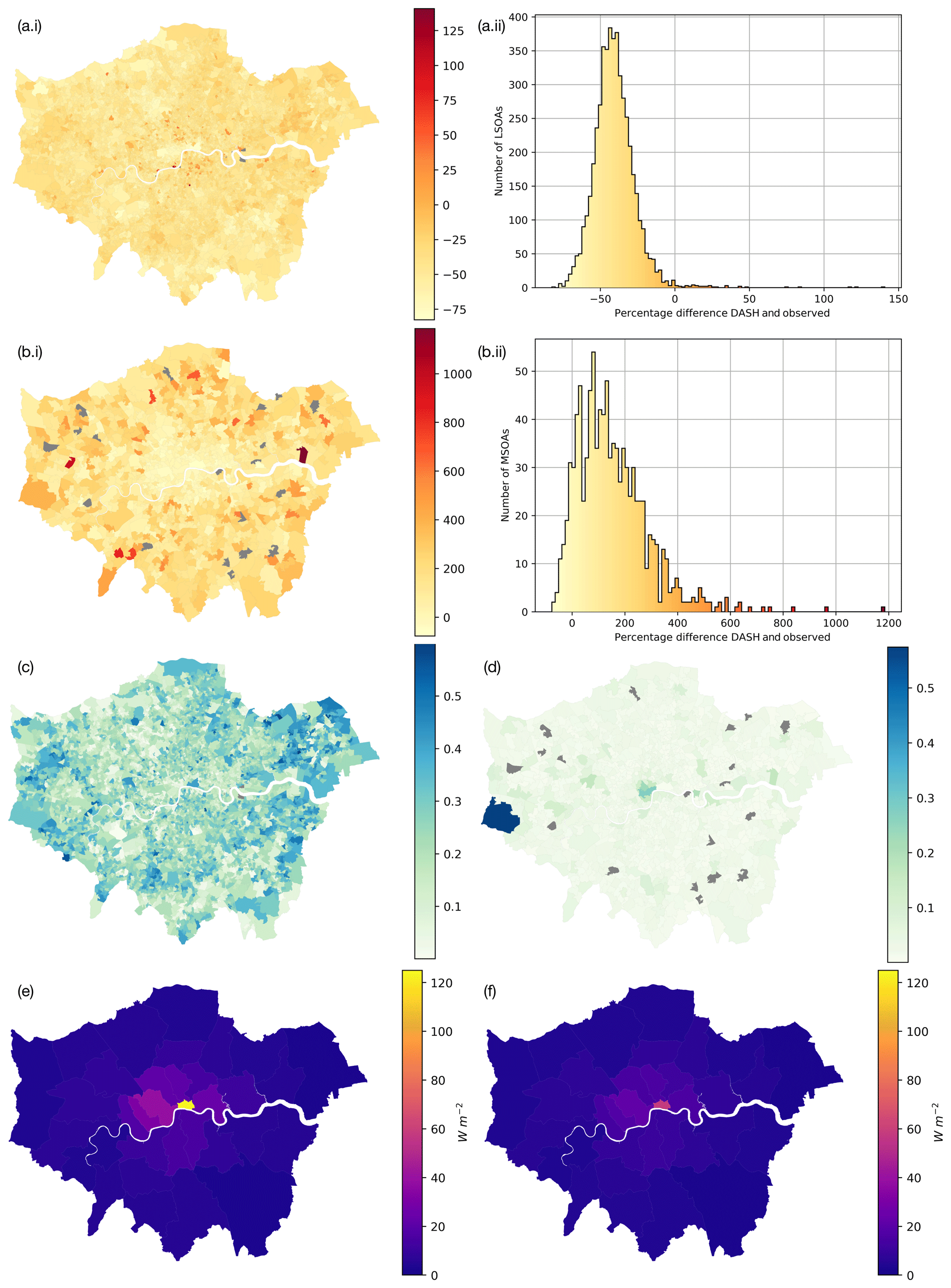
Figure 11DASH (R8, Table 6) nEi of total energy consumption represented by (i) choropleth and (ii) histogram for (a) LSOA-scale domestic use and (b) MSOA-scale commercial use. AnEi of total energy consumption for (c) LSOA-scale domestic and (d) MSOA-scale commercial. Annual average energy flux at LA scale for (e) reference data and (f) DASH.
The percentage difference between commercial DASH and non-domestic energy consumption is skewed to overestimation by DASH in most MSOAs (Fig. 11b.ii). The CBD underestimation (−53.2 %, Fig. 11b.i) is likely caused by a large misallocation of commercial gas consumption in this area (Sect. 3.2). One spatial unit (East London) overestimates by more than 1000 % (maximum being 1184 %, 24.2 GW h). Some OAs (i.e. AN scale) with large retail buildings have potential uncertainty in both the energy consumption data (e.g. undisclosed data, Sect. 3.2) and DASH simulations.
At MSOA scale, DASH simulates 38 % of the areas to within ±100 % of published values. The MSOAs that DASH most overestimates (as percentage differences) have fairly small actual magnitude differences and low workplace populations. The mean difference in magnitude across the top 5th percentile is 28.7 GW h; however 77 % of these (mean difference 18.1 GW h) have workday populations of fewer than 2000 people in the MSOA, with most businesses in these MSOAs having fewer than 50 employees. Whilst the proportion of these small businesses is fairly high (89 % on average) across Greater London (ONS, 2019), it is not the main cause of the uncertainty, as this arises from misclassification of small businesses as domestic within published data. Some overestimation occurs in areas with buildings that are not typically temperature controlled (e.g. warehouses, factories) as DASH assumes all commercial spaces are temperature controlled.
Although the percentage differences in commercial annual energy consumption are larger than for domestic (Fig. 11a.ii, b.ii), the actual commercial values (Fig. 11d) are more spatially similar across the city than domestic values (Fig. 11c). The most spatially disparate commercial area, containing Heathrow Airport (west GL, Fig. 11d), likely has undisclosed data, hence the large difference (394.7 %) of 726.8 GW h. Domestic values are more spatially similar in the less densely populated suburbs, whereas areas east of the CBD are more densely populated and more spatially variable.
The annual LA (Table 1) energy fluxes have fewer data inconsistencies when the domestic and non-domestic/commercial energy consumption are combined, allowing meter classification to be ignored. DASH QF estimates for Greater London (5.53 W m−2) are lower than those found using the published meter data (7.22 W m−2), with the greatest difference in the smallest LA, City of London (DASH gives 57.53 W m−2, and published data give 123.48 W m−2). The overall spatial patterns are similar, with greater values towards the city centre and more consistent values in the surrounding suburbs.
Although address misallocation (Sect. 3.2) is expected to cause the observed discrepancies (i.e. apparent DASH underestimation for aggregate annual values) found in the CBD, it is not possible to quantify this uncertainty. Similarly, an underestimation is expected from DASH as the meteorological input used is for one central site (Table 5), so variations (e.g. cooler temperatures or wind effects) are unaccounted for. This could be improved by coupling DASH with a meteorological model accounting for spatial heterogeneity.
DASH allows anthropogenic heat fluxes to be simulated accounting for both urban form and function, using an agent-based structure. The impact of peoples' behaviours at the neighbourhood scale is captured as occupants move (10 min time step), varying by day type (e.g. week day, weekend), demographics (e.g. age), location (e.g. residential, work, school), activity (e.g. cooking, recreation, travelling to school or work), and socio-economic factors (e.g. appliance availability) and in response to environmental conditions (e.g. temperature-related heating use). DASH includes simple transport and building energy models to allow simulation of dynamic vehicle use, occupancy, and heating–cooling demand with subsequent release of energy to the outdoor environment through the building fabric or ventilation.
Evaluation of DASH in Greater London for periods in 2015 uses a top-down inventory model (GQF) and national energy consumption statistics (as cited in Table 6, R8). Overall, the model performs well. Some of the spatial and temporal differences may be explained by data inconsistencies in the official data (e.g. privacy related, allocation of use to office headquarters rather than place of use). Analyses with DASH allow high spatial and temporal resolution for a wide range of time periods (demonstrated here from 10 min to 1 year) and large spatial extent (demonstrated from output area to megacity). The model performance evaluation addresses a wide range of these scales (e.g. 30 min spatial patterns at OA, annual at LA scale).
The expected temporal and spatial patterns of QF are obtained (e.g. two diurnal peaks and larger fluxes in the city centre). Given DASH's capabilities these can be explored and explained. For example, domestic building QF,B is more intense towards the city centre than in outer suburbs, following residential population density. The morning and evening peaks are linked to active occupancy and appliance power demand.
As DASH is demonstrated to be able to reproduce conditions generally, future work will investigate dynamic feedbacks within a city that result from changes in urban form and function. DASH is designed to allow parameters to be altered spatially, and thus impacts on QF emissions can be assessed. Changes may be both slow (i.e. over years), such as from an ageing population, uptake or new technology (e.g. change of vehicle fuels and efficiency), or governance (e.g. national energy or carbon goals), and short term (i.e. hours, days to months), resulting from traffic restrictions (e.g. roadworks, flooding) changing flows. The model performance suggests that other capabilities (e.g. additional transport types) and feedback on other variables' (e.g. CO2) emissions are warranted in the future. With DASH coupled to an urban land surface model, impacts can be assessed both on QF itself (e.g. a traffic disruption at one point in terms of the impact on QF,B) and feedbacks on other surface energy balance terms and near-surface urban temperatures. Such a model capability is critical in considering future urban climate scenarios and impacts of human behaviours and feedbacks.
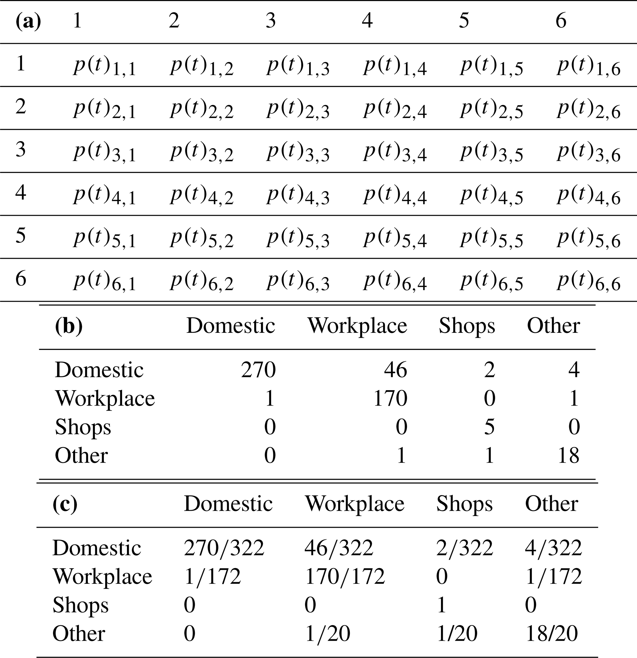
A Markov transition matrix (Hermanns, 2003; Sericola, 2013) is built from the probabilities of transition from one state to another in the next time step, with n states forming an n×n Markov transition matrix (Table A1a). Entries are the probabilities p of transitioning from one state at time step t (row) to another at time step t+1 (column) (e.g. Table A1b, c). Stationary distribution for state 1 is
The transition matrices created for this model are time inhomogeneous, reflecting a realistic diurnal profile with changes in likelihood state through the day. If state transition ”n, n” is chosen, the state does not change. Markov transition matrices may exclude entry to particular states by setting the column and row of a restricted state to zero.
As there is no way to determine the states prior to the start of a model run and to ensure no spin-up is required, the stationary distribution for the first-time step in the run is given by the diagonal of the matrix (e.g. based on the six states in Table A1):
This represents the distribution across states that are not in transition during the previous or the current time step.
For travel (Sect. 2.4.2) at t=1, OC are distributed using a weighted choice with the diagonal of the transition matrix (Eq. A2) for that time step and age group as the weight distribution. At each subsequent time step, the origin AN has a choice to keep each OC or release them into another , according to weighted choice (Eq. 3) using the transition probabilities dictated by the origin 's stationary distribution (Eq. A1) at t as ω. The AN destination depends on the destination selected. If for the next time step is the same as the previous time step, the AN does not release the OC.
Table A1Markov transition matrix (a) general for six states (rows and columns), (b) example data for adult OC at a single time step (Gershuny and Sullivan, 2017), and (c) transition probabilities for the data in (b).
STEBBS employs a nodal approach (Foucquier et al., 2013) as found in commonly used simulation tools such as TRNSYS (Klein et al., 2017) and EnergyPlus (Crawley et al., 2000). Each node represents a homogeneous layer within a specified component of the building, with heat transfer equations solved between each node (Fig. B1). STEBBS' eight nodes are two layered for wall–roof, ground floor, and windows – plus a bulk air node and an all internal mass node (calculated as a percentage of total volume). Additionally, there are six nodes associated with the domestic hot water (DHW) system. There are two layers for the hot water tank walls and a bulk DHW distribution system, plus a bulk water node for the storage and a distribution node. Effective thermal properties are applied to each component (i.e. a wall cavity and insulation layers are not modelled separately). As this is computationally cheap, it allows multiple instances for each AN at high temporal resolution. The only latent heat consideration is that of people from metabolic processes (Sect. 2.4.1).
STEBBS considers heat exchanges by convection, conduction, and radiation, and heat gain from solar insolation and casual heat sources (Fig. B1). The convective flux, qcv, between a fluid f and a surface s (Bergman et al., 2017) is
where Tf and Ts are the temperatures of the fluid (f) and surface (s), respectively, and A is the surface area of the building. Convective fluxes occur between indoor (outdoor) air and internal (external) wall/window/floor surface as well as the internal mass surface. For DHW, Eq. (B1) calculates convective flux between water and hot water tank/vessel walls. Forced convection h is experienced on external walls as a function of wind speed ws (m s−1) at roof height, so it is variable, whilst internal values are held constant (Cole and Sturrock, 1977):
Conduction between internal and external surfaces of a component (i.e. wall, window, floor, hot water tank/vessel, and ground floor to ground) is
where ke is the effective conductivity of a building component with 1 to n layers of thickness Ln (sum to L) and conductivity kn.
and Tsi and Tso are the component's inside and outside surface temperatures, respectively. This is calculated for inside surfaces of a wall, ceiling, window, floor, hot water tank, and hot water vessel components and their respective outside surfaces, as well as the point of contact between the ground floor and the external ground.
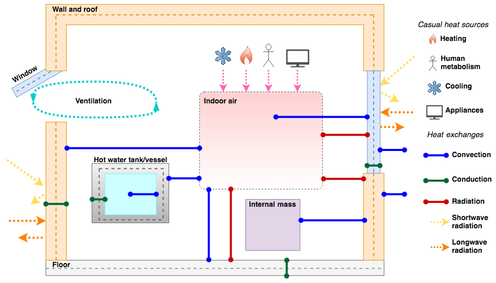
Figure B1STEBBS 1-D model simulates building facets and nodes (dots), casual heat sources, and heat exchanges. Longwave radiation is absorbed by building facets from the outdoor environment and shortwave radiation from direct, diffuse, and reflected sources.
Shortwave insolation (K↓) is considered on building walls, roof and windows, with transmitted proportion through windows added to internal heat gain and absorbed proportion contributing to wall/roof/window gains (Underwood and Yik, 2004). Windows have an effective shortwave transmissivity (τ) and albedo (Θ), whereas walls and roof depend only on their albedo. Solar internal heat gain (qsi) is
and solar gain to external wall () and window () is
The net longwave radiation (QL∗) exchange between building surfaces (walls or windows) and surfaces (including sky) in their view is found using Bergman et al. (2017):
where σ is the Stefan–Boltzmann constant ( W m−2 K−4), ε is the wall/window emissivity, and surface temperature Ts,i is the temperature of the surface (i) in view.

Figure B2BESTEST Case 600 is used with London weather data to evaluate STEBBS relative to EnergyPlus (EP) at an hourly timescale for 2012 (a) heating and (b) cooling loads (J), (c) indoor air temperature, (d) frequency distribution of hourly differences between EnergyPlus and STEBBS for heating and cooling loads, (e) interquartile range of hourly differences in winter (January, February, March, October, November, December) and summer (May, June, July, August) loads, and indoor temperatures (whiskers 1 % and 99 %).
The three view factors (ψi) for external wall/window surfaces (sky ψs, buildings ψb, and ground ψg) will sum to 1. Currently, for neither short- nor longwave radiation is ψ accounted for (i.e. uniform temperature is assumed). This could be improved when coupled with more detailed morphology data and urban meteorology as ψ varies across a city with height (building facet) and density of buildings (Grimmond et al., 2001). Internal wall radiative exchanges are currently not considered.
Energy for heating (cooling) is controlled by setpoint temperature with energy added (removed) directly from the indoor air node that is controlled according to a maximum power rating and set system efficiency. The temperature setpoints can change at each time step, allowing both automated and human control to be accounted for. The level of heating (cooling) is further controlled by the difference between indoor air and setpoint temperatures. Internal gains are accounted for as a bulk gain to the indoor air node.
The BESTEST Case 600 single-zone building case is used with EnergyPlus (v.9.3.0). to evaluate STEBBS. The EnergyPlus BESTEST model downloaded from the EnergyPlus helpserve website (EnergyPlus, 2020) is modified to run with v9.3.0. Observed London weather data for 2012 (Kotthaus and Grimmond, 2014) are generated using SuPy (Sun and Grimmond, 2019) at an hourly resolution for EnergyPlus and STEBBS. Although EnergyPlus indicates it interpolates sub-hourly weather data for consistency, we use both with a 1 h time step.
Following EnergyPlus Engineering Reference, the STEBBS external convection coefficient is changed to the DOE-2 method (U.S. Department of Energy, 2020, pp. 95–96) for consistency between the models. Note, this is found to have little impact on the results. The internal mass and DHW in STEBBS are reduced in volume to ensure they have negligible impact on results (see https://doi.org/10.5281/zenodo.3745523, Capel-Timms et al., 2020, for BESTEST setup). The bulk building thermal properties in STEBBS are calculated using the BESTEST Case 600 values as presented in ASHRAE 140 (ASHRAE, 2017). Building dimensions for STEBBS are set to give consistent total indoor volume, wall–roof surface area, window area, and floor area. As STEBBS has only one pair of nodes (i.e. two-layer wall; Fig. B1), building geometry and orientation are not represented in STEBBS.
The EnergyPlus annual and inter-day heating and cooling dynamics are captured in STEBBS (Fig. B2). Both models control the indoor air temperature to within the setpoint limits of 20 ∘C (heating) and 27 ∘C (cooling). EnergyPlus simulates a higher heating and cooling load with more times when the indoor temperature is between (rather than at) the setpoint temperatures. EnergyPlus also simulates a cooling requirement during the heating season, which STEBBS does not.
The modal hourly heating–cooling load differences between the two models are relatively small (Fig. B2). Although the distribution range is large, the differences are perhaps best attributed to a difference in load control. The EnergyPlus BESTEST case uses the maximum heating (cooling) capacity to add (remove) thermal energy to (from) the building that is likely to result in the observed indoor temperature overshoots, the higher frequency of switching (on–off) for heating and cooling, and need for cooling during heating season as heating and cooling power are set high (100 kW) – to prevent this type of behaviour, STEBBS uses the difference between air and setpoint temperature to help control the heating and cooling power.
Table C1Appliances used in domestic and workplace subareas and their attributes. Usage categories: active only (AO) consume energy as a result of user activities; active with standby (AS) consume less when not in active use (standby); continuous (C) have constant power consumption independent of human activity (cycling appliance power converted to continuous). See Table 3 for references.
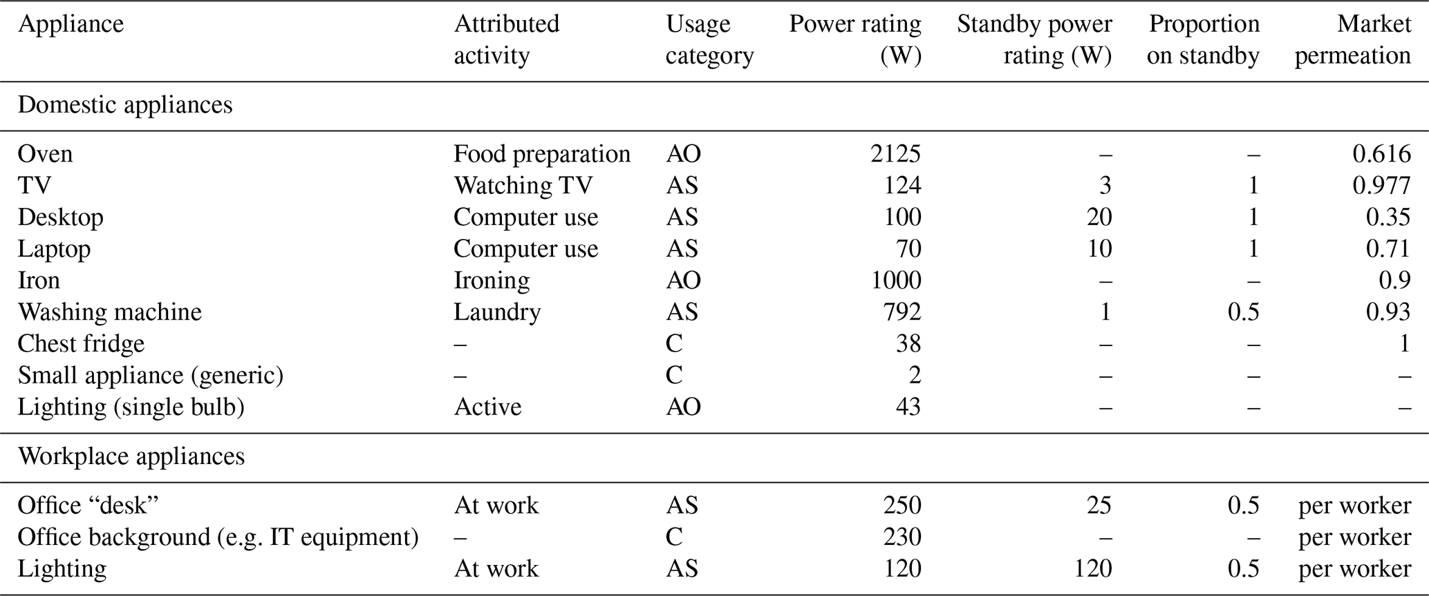
Table C2Properties used in STEBBS vary by property age (<1965, >1965), type (HB – house & bungalow; flat), component (roof etc.) for (a) building fabric and external ground, and (b) DHW. L: thickness (m); ε: emissivity; τ: effective transmissivity; Θ: surface albedo; ke: effective thermal conductivity (); ρ: density (kg m−3); cp: specific heat of air at constant pressure () (Internal Air 1005); h: convection coefficient (Int: internal, Ext: external) (); VFR: volumetric flow rate of DHW per water user (dom: domestic, n-dom: non-domestic) (10−3 m3 s−1); VR: ventilation rate (10−3 m3 s−1); VT: DHW tank volume (m3); WWR: window-to-wall ratio (0.4). Vessels: all other storage of DHW. For data sources refer to Table 3.
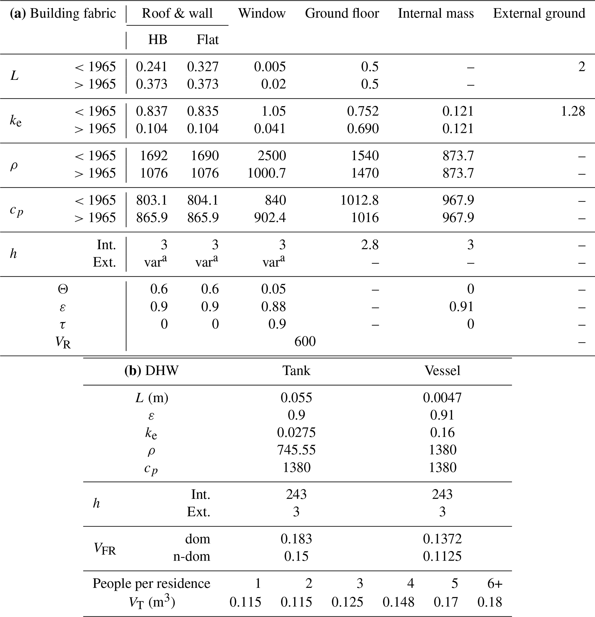
a Varies with wind speed.
All code and data are deposited at
https://doi.org/10.5281/zenodo.3745523 (Capel-Timms et al., 2020).
Table D1Data examples. More details (example structure, units, raw data source, location in repository, and location of use in code) can be found at https://doi.org/10.5281/zenodo.3745523 (Capel-Timms et al., 2020). Data indicated in Table 6 are also archived.

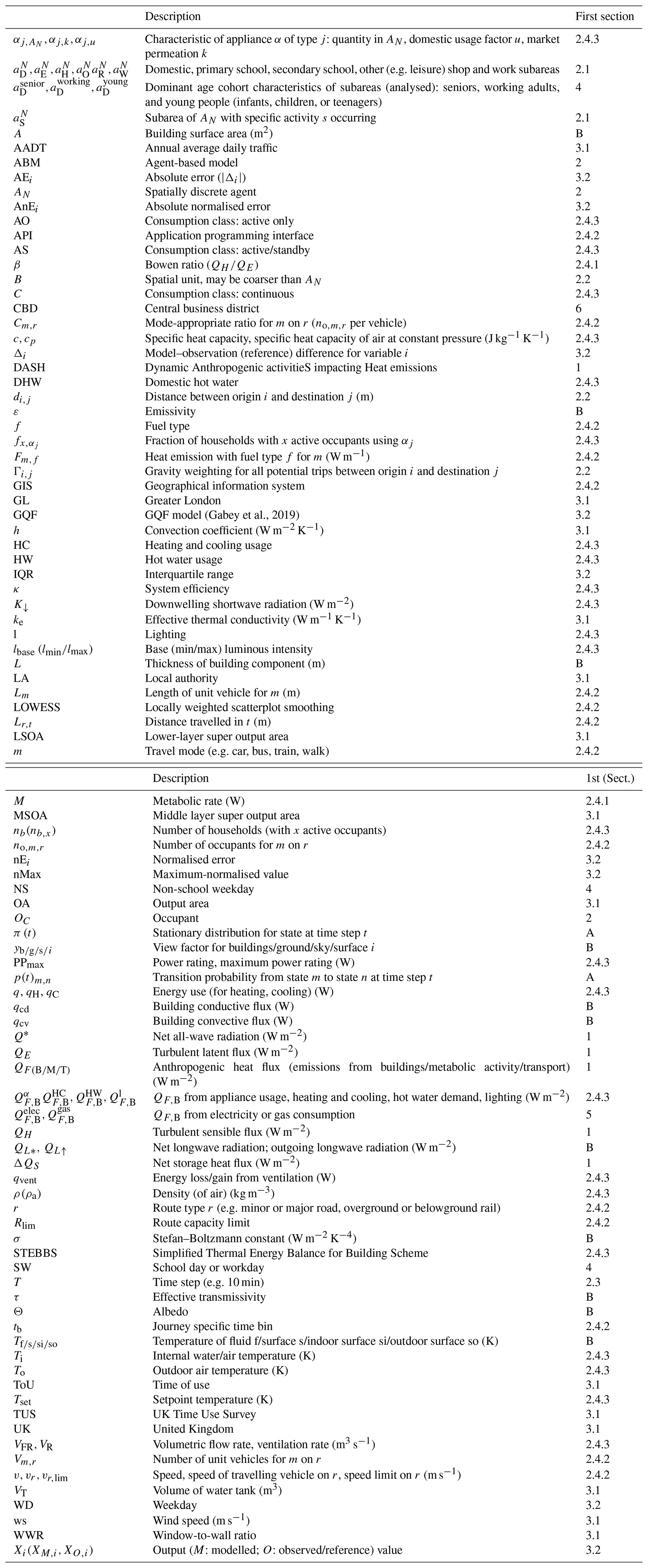
All code and data are deposited at https://doi.org/10.5281/zenodo.3745523 (Capel-Timms et al., 2020).
The project was conceptualised by SG, STS, and ICT. ICT, STS, TS, and SG developed the methods. ICT, TS, STS, and SG undertook the analyses. ICT wrote the first draft and created the figures. SG, STS, ICT, and TS reviewed and edited the paper for submission. Resources were supplied by SG and STS. This project was conducted as part of a PhD with supervision from SG, STS, and TS.
The authors declare that they have no conflict of interest.
Andy Gabey provided support in early development of DASH and adaptation of GQF for evaluation purposes. George Meachim carried out the gap filling for use of meteorological data. We acknowledge Ian Hamilton (UCL) for some building parameters.
This work has been funded by EPSRC (University of Reading doctoral training grant), NERC APEx (grant no. NE/T001887/1), NERC Independent Research Fellowship (grant no. NE/P018637/1), Newton Fund/Met Office CSSP China for Sue Grimmond and Isabella Capel-Timms (grant no. AJYG-DX4P1V), and ERC urbisphere (grant no. 855005).
This paper was edited by David Lawrence and reviewed by two anonymous referees.
Allen, L., Lindberg, F., and Grimmond, C. S. B.: Global to city scale urban anthropogenic heat flux: model and variability, Int. J. Climatol., 31, 1990–2005, 2011.
ASHRAE: ANSI/ASHRAE Standard 140-2017, Standard Method of Test for the Evaluation of Building Energy Analysis Computer Programs, 2017.
Baetens, R. and Saelens, D.: Modelling uncertainty in district energy simulations by stochastic residential occupant behaviour, J. Build. Perform. Simu., 9, 431–447, https://doi.org/10.1080/19401493.2015.1070203, 2016.
BCO: Guide to Specification 2009, British Council for Offices, 2009.
BEIS: Department for Business, Energy & Industrial Strategy: Sub-national electricity consumption data, available at: https://www.gov.uk/government/collections/sub-national-electricity-consumption-data#lsoa/msoa-data, last access: 14 July 2017a.
BEIS: Department for Business, Energy & Industrial Strategy: Sub-national gas consumption data, available at: https://www.gov.uk/government/collections/sub-national-gas-consumption-data, last access: 14 July 2017b.
BEIS: Department for Business, Energy & Industrial Strategy: Sub-national total final energy consumption data, available at: https://www.gov.uk/government/collections/total-final-energy-consumption-at-sub-national-level, last access: 14 July 2017c.
BEIS: Department for Business, Energy & Industrial Strategy: Sub-National Consumption Statisitics: Methodology and guidance booklet, 2018.
Bergman, T. L., Lavine, A. S., Incropera, F. P., and DeWitt, D. P.: Fundamentals of Heat and Mass Transfer, 8th Edn., Wiley Global Education, 2017.
Best, M. J. and Grimmond, C. S. B.: Investigation of the impact of anthropogenic heat flux within an urban land surface model and PILPS-urban, Theor. Appl. Climatol., 126, 51–60, https://doi.org/10.1007/s00704-015-1554-3, 2016.
Björkegren, A. and Grimmond, C. S. B.: Net carbon dioxide emissions from central London, Urban Clim., 23, 131–158, https://doi.org/10.1016/j.uclim.2016.10.002, 2018.
Blitzstein, J. K. and Hwang, J.: Introduction to Probability, 2nd Edn., Chapman and Hall, CRC Press, 2019.
Bohnenstengel, S. I., Hamilton, I., Davies, M., and Belcher, S. E.: Impact of anthropogenic heat emissions on London's temperatures, Q. J. Roy. Meteor. Soc., 140, 687–698, https://doi.org/10.1002/qj.2144, 2014.
BSI: BS 6700: Specification for Design, installation, testing and maintenance of services supplying water for domestic use within buildings and their curtilages, British Standards Institution, 1997.
Bueno, B., Pigeon, G., Norford, L. K., Zibouche, K., and Marchadier, C.: Development and evaluation of a building energy model integrated in the TEB scheme, Geosci. Model Dev., 5, 433–448, https://doi.org/10.5194/gmd-5-433-2012, 2012.
Busby, J.: UK shallow ground temperatures for ground coupled heat exchangers, Q. J. Eng. Geol. Hydroge., 48, 248–260, https://doi.org/10.1144/qjegh2015-077, 2015.
Butcher, K. (Ed.): CIBSE Guide K: Electricity in buildings, Chartered Institution of Building Services Engineers, 2004.
Butcher, K. (Ed.): CIBSE Guide F: Energy Efficiency in Buildings, Chartered Institution of Building Services Engineers, 2012.
Butcher, K. (Ed.): CIBSE Guide G: Public health and plumbing engineering, Chartered Institute of Building Service Engineers, 2014.
Butcher, K. and Craig, B. (Eds.): CIBSE Guide A: Environmental design, Chartered Institute of Building Service Engineers, London, 2016.
Casey, H. J.: The law of retail gravitation applied to traffic engineering, Traffic Q., 9, 313–321, 1955.
Capel-Timms, I., Smith, S. T., Sun, T., and Grimmond, S.: Dynamic Anthropogenic activitieS impacting Heat emissions (DASH v1.0): Development and evaluation (Version 1.2), Zenodo, https://doi.org/10.5281/zenodo.3936025, 2020.
Chrysoulakis, N., Grimmond, S., Feigenwinter, C., Lindberg, F., Gastellu-Etchegorry, J. P., Marconcini, M., Mitraka, Z., Stagakis, S., Crawford, B., Olofson, F., Landier, L., Morrison, W., and Parlow, E.: Urban energy exchanges monitoring from space, Sci. Rep., 8, 1–8, https://doi.org/10.1038/s41598-018-29873-x, 2018.
Cleveland, W. S.: LOWESS: A Program for Smoothing Scatterplots by Robust Locally Weighted Regression, Am. Stat., 35, 54, https://doi.org/10.2307/2683591, 1988.
Cole, R. J. and Sturrock, N. S.: The convective heat exchange at the external surface of buildings, Build. Environ., 12, 207–214, https://doi.org/10.1016/0360-1323(77)90021-X, 1977.
Crawford, B., Grimmond, C. S. B., Ward, H. C., Morrison, W., and Kotthaus, S.: Spatial and temporal patterns of surface–atmosphere energy exchange in a dense urban environment using scintillometry, Q. J. Roy. Meteor. Soc., 143, 817–833, https://doi.org/10.1002/qj.2967, 2017.
Crawley, D. B., Lawrie, L. K., Pedersen, C. O., and Winkelmann, F. C.: EnergyPlus: Energy Simulation Program, ASHRAE J., 42, 49–56, 2000.
Crooks, A. T. and Heppenstall, A. J.: Introduction to Agent-Based Modelling, in: Agent-Based Models of Geographical Systems, 85–105, 2012.
DECC: Non-Domestic National Energy Efficiency Data-Framework: Energy Statistics 2006-12, Department of Energy and Climate Change, available at: https://www.gov.uk/government/statistics/non-domestic-national-energy-efficiency-data-framework-energy-statistics-2006-12 (last access: 11 February 2020), 2015.
DECC and BRE: Energy Follow Up Survey (EFUS) 2011, Department of Energy and Climate Change and Building Research Establishment, available at: https://www.gov.uk/government/statistics/energy-follow-up-survey-efus-2011 (last access: 11 February 2020), 2016.
de Munck, C., Pigeon, G., Masson, V., Meunier, F., Bousquet, P., Tréméac, B., Merchat, M., Poeuf, P., and Marchadier, C.: How much can air conditioning increase air temperatures for a city like Paris, France?, Int. J. Climatol., 33, 210–227, https://doi.org/10.1002/joc.3415, 2013.
DfE: Schools, Pupils and their Characteristics, January 2019 – Accompanying Table, Department for Education, available at: https://www.gov.uk/government/statistics/schools-pupils-and-their-characteristics-january-2019 (last access: 11 February 2020), 2019.
DfT: Department for Transport, TRA0203 – Motor vehicle traffic (vehicle kilometres) by road class and region and country in Great Britain, annual 2014, available at: https://www.gov.uk/government/statistical-data-sets/road-traffic-statistics-tra (last access: 10 February 2016), 2014a.
DfT: Department for Transport, TRA0204 – Road traffic (vehicle kilometres) by vehicle type and road class in Great Britain, annual 2014, available at: https://www.gov.uk/government/statistical-data-sets/road-traffic-statistics-tra (last access: 10 February 2016), 2014b.
DfT: Department for Transport, National Travel Survey, 2002–2016, [data collection], 12th Edn., UK Data Service, SN: 5340, https://doi.org/10.5255/UKDA-SN-5340-8, 2017.
DfT and DVLA: Department for Transport (DfT) and Driver and Vehicle Licensing Agency (DVLA), Data on all licensed and registered vehicles (VEH01), available at: https://www.gov.uk/government/statistical-data-sets/all-vehicles-veh01 (last access: 10 February 2020), 2019.
Dong, Y., Varquez, A. C. G., and Kanda, M.: Global anthropogenic heat flux database with high spatial resolution, Atmos. Environ., 150, 276–294, https://doi.org/10.1016/j.atmosenv.2016.11.040, 2017.
Druckman, A. and Jackson, T.: Household energy consumption in the UK: A highly geographically and socio-economically disaggregated model, Energ. Policy, 36, 3167–3182, https://doi.org/10.1016/j.enpol.2008.03.021, 2008.
EnergyPlus: Knowledgebase: Downloads, Testing and validation, ANSI/ASHRAE Standard 140 models, Knowledgebase Downloads, available at: http://energyplus.helpserve.com/Knowledgebase/List/Index/49, last access: 30 June 2020.
Evans, S., Liddiard, R., and Steadman, P.: Modelling a whole building stock: domestic, non-domestic and mixed use, Build. Res. Inf., 47, 156–172, https://doi.org/10.1080/09613218.2017.1410424, 2019.
Ferreira, M. J., de Oliveira, A. P., and Soares, J.: Anthropogenic heat in the city of São Paulo, Brazil, Theor. Appl. Climatol., 104, 43–56, https://doi.org/10.1007/s00704-010-0322-7, 2011.
Field, J.: TM46: Energy Benchmarks, Chartered Institute of Building Service Engineers, 2008.
Firth, S., Lomas, K., Wright, A., and Wall, R.: Identifying trends in the use of domestic appliances from household electricity consumption measurements, Energ. Buildings, 40, 926–936, https://doi.org/10.1016/j.enbuild.2007.07.005, 2008.
Fisher, K. and Gershuny, J.: Coming full circle – introducing the multinational Time Use Study Simple File, Electron. Int. J. Time Use Res., 10, 91–96, https://doi.org/10.1016/j.physbeh.2017.03.040, 2013.
Flamco: Indirect Water Heaters (mains water systems), available at: https://flamcogroup.com/media/files/documentation/EXP17_PSTEST_LR_v09022017_Chapter_6.pdf (last access: 7 March 2019), 2017.
Foucquier, A., Robert, S., Suard, F., Stéphan, L., and Jay, A.: State of the art in building modelling and energy performances prediction: A review, Renew. Sust. Energ Rev., 23, 272–288, https://doi.org/10.1016/j.rser.2013.03.004, 2013.
Gabey, A. M., Grimmond, C. S. B., and Capel-Timms, I.: Anthropogenic heat flux: advisable spatial resolutions when input data are scarce, Theor. Appl. Climatol., 135, 791–807, https://doi.org/10.1007/s00704-018-2367-y, 2019.
Gershuny, J. and Sullivan, O.: United Kingdom Time Use Survey, 2014–2015, [data collection], UK Data Service, SN: 8128, https://doi.org/10.5255/UKDA-SN-8128-1, 2017.
GLA: Greater London Authority, Statistical GIS Boundary Files for London, available at: https://data.london.gov.uk/dataset/statistical-gis-boundary-files-london (last access: 11 February 2020), 2011.
GLA: Greater London Authority, London Schools Atlas, available at: https://data.london.gov.uk/dataset/london-schools-atlas (last access: 7 September 2020), 2014.
Google: Google Directions API, available at: https://developers.google.com/maps/documentation/directions/start (last access: 31 January 2020), 2019.
Greenshields, B. D., Bibbins, J. R., Channing, W. S., and Miller, H. H.: A Study of Traffic Capacity, in Proceedings of the highway research board, Highway Research Board, Washington, D. C., 14, 448–477, 1935.
Grimmond, C. S. B.: The Suburban Energy Balance?: Methodological Considerations and Results for a Mid-Latitude West, Int. J., 12, 481–497, https://doi.org/10.1002/joc.3370120506, 1992.
Grimmond, C. S. B. and Oke, T. R.: Aerodynamic properties of urban areas derived from analysis of surface form, J. Appl. Meteorol., 38, 1262–1292, https://doi.org/10.1175/1520-0450(1999)038<1262:apouad>2.0.co;2, 1999.
Grimmond, C. S. B., Cleugh, H. A., and Oke, T. R.: An objective urban heat storage model and its comparison with other schemes, Atmos. Environ., 25, 311–326, https://doi.org/10.1016/0957-1272(91)90003-W, 1991.
Grimmond, C. S. B., Potter, S. K., Zutter, H. N., and Souch, C.: Rapid methods to estimate sky view factors applied to urban areas, Int. J. Climatol., 21, 903–913, https://doi.org/10.1002/joc.659, 2001.
Hawkins, G.: Rules of Thumb, Guidelines for Building Services, 5th Edn., BSRIA, Building Services Research and Information Association, 2011.
HCA: Employment Densities Guide: 2nd Edition, Homes and Communities Agency, available at: https://www.gov.uk/government/publications/employment-densities-guide (last access: 7 September 2020), 2010.
Heaviside, C., Vardoulakis, S., and Cai, X.-M.: Attribution of mortality to the urban heat island during heatwaves in the West Midlands, UK, Environ. Health, 15 Suppl 1, 50–59, https://doi.org/10.1186/s12940-016-0100-9, 2016.
Heiple, S. and Sailor, D. J.: Using building energy simulation and geospatial modeling techniques to determine high resolution building sector energy consumption profiles, Energ. Buildings, 40, 1426–1436, https://doi.org/10.1016/j.enbuild.2008.01.005, 2008.
Hermanns, H.: Interactive Markov Chains: The Quest for Quantified Quality, Springer, 2003.
Highways Agency: Traffic Capcity of Urban Roads. Design Manual for Roads and Bridges: TA 79/99, Highways Agency, available at: http://www.standardsforhighways.co.uk/ha/standards/dmrb/vol5/section1/ta7999.pdf (last access: 10 February 2020), 2017.
Hinkel, K. M., Nelson, F. E., Klene, A. E., and Bell, J. H.: The urban heat island in winter at Barrow, Alaska, Int. J. Climatol., 23, 1889–1905, https://doi.org/10.1002/joc.971, 2003.
Iamarino, M., Beevers, S., and Grimmond, C. S. B.: High-resolution (space, time) anthropogenic heat emissions: London 1970–2025, Int. J. Climatol., 32, 1754–1767, https://doi.org/10.1002/joc.2390, 2012.
IOP: Institute of Plumbing. Plumbing Services Engineering Design Guide ISBN 9781871956405, 2002.
Kikegawa, Y., Genchi, Y., Yoshikado, H., and Kondo, H.: Development of a numerical simulation system toward comprehensive assessments of urban warming countermeasures including their impacts upon the urban buildings' energy-demands, Appl. Energ., 76, 449–466, https://doi.org/10.1016/S0306-2619(03)00009-6, 2003.
Kikegawa, Y., Tanaka, A., Ohashi, Y., Ihara, T., and Shigeta, Y.: Observed and simulated sensitivities of summertime urban surface air temperatures to anthropogenic heat in downtown areas of two Japanese Major Cities, Tokyo and Osaka, Theor. Appl. Climatol., 117, 175–193, https://doi.org/10.1007/s00704-013-0996-8, 2014.
Kim, Y. S. and Srebric, J.: Impact of occupancy rates on the building electricity consumption in commercial buildings, Energ. Buildings, 138, 591–600, https://doi.org/10.1016/j.enbuild.2016.12.056, 2017.
Klein, S. A., Duffie, J. A., and Mitchell, J. C.: TRNSYS 18: A Transient System Simulation Program, Solar Energy Laboratory, University of Wisconsin, available at: https://sel.me.wisc.edu/trnsys/ (last access: 31 January 2020), 2017.
Knudsen, S.: Heat transfer in a “tank in tank” combi store, BYG Rapport, No. R-025, 2002.
Kotthaus, S. and Grimmond, C. S. B.: Identification of Micro-scale Anthropogenic CO2, heat and moisture sources – Processing eddy covariance fluxes for a dense urban environment, Atmos. Environ., 57, 301–316, https://doi.org/10.1016/j.atmosenv.2012.04.024, 2012.
Kotthaus, S. and Grimmond, C. S. B.: Energy exchange in a dense urban environment – Part I: Temporal variability of long-term observations in central London, Urban Clim., 10, 261–280, https://doi.org/10.1016/j.uclim.2013.10.002, 2014.
Lee, S. H., Song, C. K., Baik, J. J., and Park, S. U.: Estimation of anthropogenic heat emission in the Gyeong-In region of Korea, Theor. Appl. Climatol., 96, 291–303, https://doi.org/10.1007/s00704-008-0040-6, 2009.
LGA: Local Government Association website, available at: https://www.local.gov.uk/about/what-local-government, last access: 26 November 2019.
Lindberg, F., Grimmond, C. S. B., Yogeswaran, N., Kotthaus, S., and Allen, L.: Impact of city changes and weather on anthropogenic heat flux in Europe 1995–2015, Urban Clim., 4, 1–15, https://doi.org/10.1016/j.uclim.2013.03.002, 2013.
London Datastore: London Atmospheric Emissions Inventory (LAEI) 2013 – Supporting information: key GIS geographies and road traffic flows and vehicle-kilometres, available at: https://data.london.gov.uk/dataset/london-atmospheric-emissions-inventory-2013 (last access: 11 February 2020), 2014.
Lu, Y., Wang, Q., Zhang, Y., Sun, P., and Qian, Y.: An estimate of anthropogenic heat emissions in China, Int. J. Climatol., 36, 1134–1142, https://doi.org/10.1002/joc.4407, 2016.
Macal, C. and North, M.: Tutorial on agent-based modelling and simulation, J. Simul., 4, 151–162, https://doi.org/10.1057/jos.2010.3, 2010.
Mavrogianni, A., Wilkinson, P., Davies, M., Biddulph, P., and Oikonomou, E.: Building characteristics as determinants of propensity to high indoor summer temperatures in London dwellings, Build. Environ., 55, 117–130, https://doi.org/10.1016/j.buildenv.2011.12.003, 2012.
McKenna, E., Krawczynski, M., and Thomson, M.: Four-state domestic building occupancy model for energy demand simulations, Energ. Buildings, 96, 30–39, https://doi.org/10.1016/j.enbuild.2015.03.013, 2015.
MWS: McDonald Water Storage Ltd: Hot Water Tanks Specifications and Sizing, available at: https://www.mcdonaldwaterstorage.com/rectangular-tank-sizing-specifications, last access: 7 March 2019.
National Bureau of Statistics of China: China Statistical Information Network, available at: http://www.stats.gov.cn/english/statisticaldata/censusdata/ (last access: 11 February 2020), 2017.
NG: National Grid: Transmission operational data, available at: https://www.nationalgridgas.com/data-and-operations/transmission-operational-data, last access: 28 November 2015.
Nie, W. S., Sun, T., and Ni, G. H.: Spatiotemporal characteristics of anthropogenic heat in an urban environment: A case study of Tsinghua Campus, Build. Environ., 82, 675–686, https://doi.org/10.1016/j.buildenv.2014.10.011, 2014.
Offerle, B., Grimmond, C. S. B., and Fortuniak, K.: Heat storage and anthropogenic heat flux in relation to the energy balance of a central European city centre, Int. J. Climatol., 25, 1405–1419, https://doi.org/10.1002/joc.1198, 2005.
Oke, T. R.: The urban energy balance, Prog. Phys. Geogr., 12, 471–508, https://doi.org/10.1177/030913338801200401, 1988.
ONS: Office for National Statistics, QS406EW – Household size, available at: https://www.nomisweb.co.uk/census/2011/qs406ew (last access: 10 February 2020), 2011.
ONS: Office for National Statistics, WP101EW Population (Workplace population), available at: https://www.nomisweb.co.uk/query/construct/summary.asp?reset=yes&mode=construct&dataset=1300&version=0&anal=1&initsel=%0D (last access: 31 January 2020), 2014a.
ONS: Office for National Statistics, WU03UK Location of usual residence and place of work by method of travel to work, available at: https://www.nomisweb.co.uk/query/construct/summary.asp?reset=yes&mode=construct&dataset=1207&version=0&anal=1&initsel= (last access: 31 January 2020), 2014b.
ONS: Office for National Statistics, Mid-2015 Population Estimates for Census Output Areas in London by Single Year of Age and Sex, available at: https://www.ons.gov.uk/peoplepopulationandcommunity/populationandmigration/populationestimates/datasets/censusoutputareaestimatesinthelondonregionofengland, last access: 25 May 2015.
ONS: Office for National Statistics, Census Geography, available at: https://www.ons.gov.uk/methodology/geography/ukgeographies/censusgeography, last access: 11 February 2017a.
ONS: Office for National Statistics, Labour force survey – Families and Households, available at: https://www.ons.gov.uk/peoplepopulationandcommunity/birthsdeathsandmarriages/families/datasets/familiesandhouseholdsfamiliesandhouseholds, last access: 30 October 2017b.
ONS: Estimated average calorific values of fuels 2017 – Digest of UK Energy Statistics (DUKES): calorific values, available at: https://www.gov.uk/government/statistics/dukes-calorific-values (last access: 31 January 2020), 2018.
ONS: Office for National Statistics, UK Business Counts – local units by industry and employment size band, available at: https://www.nomisweb.co.uk/datasets/idbrlu (last access: 17 January 2020), 2019.
OpenStreetMap: OpenStreetMap data of Greater London, available at: https://www.openstreetmap.org, last access: 31 January 2017.
OS: OS MasterMap®, available at: http://digimap.edina.ac.uk (last access: 11 October 2015), 2014.
OS: London digital speed limit map and private communication, Ordnance Survey, 2015.
OS: OS Open Roads, available at: https://www.ordnancesurvey.co.uk/opendatadownload/products.html (last access: 30 August 2016), 2016.
O'Sullivan, D., Millington, J., Perry, G., and Wainwright, J.: Agent-Based Models – Because They're Worth It?, in: Agent-Based Models of Geographical Systems, 109–123, 2012.
Page, J., Robinson, D., Morel, N., and Scartezzini, J. L.: A generalised stochastic model for the simulation of occupant presence, Energ. Buildings, 40, 83–98, https://doi.org/10.1016/j.enbuild.2007.01.018, 2008.
Palmer, E. (Ed.): CIBSE Guide B1: Heating, Chartered Institution of Building Services Engineers, 2016.
Pigeon, G., Legain, D., Durand, P., and Masson, V.: Anthropogenic heat release in an old European agglomeration (Toulouse, France), Int. J. Climatol., 27, 1969–1981, 2007.
Reilly, W. J.: The Law of Retail Gravitation (1931), 2nd Edn., Pilsbury Publishers, New York, 1953.
Richardson, I., Thomson, M., and Infield, D.: A high-resolution domestic building occupancy model for energy demand simulations, Energ. Buildings, 40, 1560–1566, https://doi.org/10.1016/j.enbuild.2008.02.006, 2008.
Richardson, I., Thomson, M., Infield, D., and Clifford, C.: Domestic electricity use: A high-resolution energy demand model, Energ. Buildings, 42, 1878–1887, https://doi.org/10.1016/j.enbuild.2010.05.023, 2010.
Sailor, D. J.: A review of methods for estimating anthropogenic heat and moisture emissions in the urban environment, Int. J. Climatol., 31, 189–199, https://doi.org/10.1002/joc.2106, 2011.
Sailor, D. J. and Lu, L.: A top-down methodology for developing diurnal and seasonal anthropogenic heating profiles for urban areas, Atmos. Environ., 38, 2737–2748, https://doi.org/10.1016/j.atmosenv.2004.01.034, 2004.
Salamanca, F. P., Georgescu, M., Mahalov, A., Moustaoui, M., and Wang, M.: Anthropogenic heating of the urban environment due to air conditioning, J. Geophys. Res.-Atmos., 119, 5949–5965, https://doi.org/10.1002/2013jd021225, 2014.
Salter, R. J.: The relationship between space, flow and density of a highway traffic stream, in: Highway Traffic Analysis and Design, Palgrave Macmillan, 119–120, 1989.
Santamouris, M., Papanikolaou, N., Livada, I., Koronakis, I., Georgakis, C., Argiriou, A., and Assimakopoulos, D. N.: On the impact of urban climate on the energy consumption of buildings, Sol. Energy, 70, 201–216, https://doi.org/10.1016/S0038-092X(00)00095-5, 2001.
Schoetter, R., Masson, V., Bourgeois, A., Pellegrino, M., and Lévy, J.-P.: Parametrisation of the variety of human behaviour related to building energy consumption in the Town Energy Balance (SURFEX-TEB v. 8.2), Geosci. Model Dev., 10, 2801–2831, https://doi.org/10.5194/gmd-10-2801-2017, 2017.
SciPy: Numpy random sampling, available at: https://docs.scipy.org/doc/numpy/reference/random/index.html, last access: 30 November 2019.
Sellers, W. D.: Physical Climatology, 4th Edn., Univeristy of Chicago Press, Ltd, 1972.
Sericola, B.: Markov chains: theory, algorithms and applications, John Wiley & Sons, Inc., 2013.
Smith, C., Lindley, S. and Levermore, G.: Estimating spatial and temporal patterns of urban anthropogenic heat fluxes for UK cities: The case of Manchester, Theor. Appl. Climatol., 98, 19–35, https://doi.org/10.1007/s00704-008-0086-5, 2009.
Spitler, J. D.: Thermal Load and Energy performance prediction, in: Building performance simulation for design and operation, edited by: Hensen, J. L. and Lamberts, R., Spon Press, 2011.
Statistics Bureau of Japan: Japanese census data resolution, available at: https://www.stat.go.jp/english/data/index.html (last access: 7 September 2020), 2017.
Statistics Canada: Statistical Area Classification (SAC), available at: https://www150.statcan.gc.ca/n1/pub/92-195-x/2016001/other-autre/sac-css/sac-css-eng.htm (last access: 11 February 2020), 2017.
Steadman, P., Bruhns, H. R., and Rickaby, P. A.: An introduction to the national Non-Domestic Building Stock database, Environ. Plann. B, 27, 3–10, https://doi.org/10.1068/bst2, 2000.
Stewart, I. D., Oke, T. R., and Krayenhoff, E. S.: Evaluation of the “local climate zone” scheme using temperature observations and model simulations, Int. J. Climatol., 34, 1062–1080, https://doi.org/10.1002/joc.3746, 2014.
Sun, T. and Grimmond, S.: A Python-enhanced urban land surface model SuPy (SUEWS in Python, v2019.2): development, deployment and demonstration, Geosci. Model Dev., 12, 2781–2795, https://doi.org/10.5194/gmd-12-2781-2019, 2019.
TfL: Transport for London. Bus service usage, passengers and kilometres operated by route (2014–2015), available at: https://tfl.gov.uk/corporate/publications-and-reports/buses#on-this-page-1 (last access: 12 February 2020), 2018.
TfL: Transport for London. Number of Buses by Type of Bus in London, available at: https://data.london.gov.uk/dataset/number-buses-type-bus-london (last access: 11 February 2020), 2019.
Thorsson, S., Rocklöv, J., Konarska, J., Lindberg, F., Holmer, B., Dousset, B., and Rayner, D.: Mean radiant temperature – A predictor of heat related mortality, Urban Clim., 10, 332–345, https://doi.org/10.1016/j.uclim.2014.01.004, 2014.
Underwood, C. P. and Yik, F.: Modelling methods for energy in buildings, Blackwell Publishing, Malden, 2004.
U.S. Department of Energy: EnergyPlusVersion 9.3.0: Engineering Reference, 2020.
US Census Bureau: US Census Geography, available at: https://www.census.gov/data.html (last access: 11 February 2020), 2019.
VOA: Dwellings by Property Build Period and Type, available at: https://data.london.gov.uk/dataset/property-build-period-lsoa (last access: 31 January 2020), 2015.
Ward, H. C. and Grimmond, C. S. B.: Assessing the impact of changes in surface cover, human behaviour and climate on energy partitioning across Greater London, Landscape Urban Plan., 165, 142–161, 2017.
Ward, H. C., Kotthaus, S., Järvi, L., and Grimmond, C. S. B.: Surface Urban Energy and Water Balance Scheme (SUEWS): Development, Evaluation and Application, Urban Clim., 18, 1–32, https://doi.org/10.1016/j.uclim.2016.05.001, 2016.
Widén, J. and Wäckelgård, E.: A high-resolution stochastic model of domestic activity patterns and electricity demand, Appl. Energ., 87, 1880–1892, https://doi.org/10.1016/j.apenergy.2009.11.006, 2010.
Widén, J., Nilsson, A. M., and Wäckelgård, E.: A combined Markov-chain and bottom-up approach to modelling of domestic lighting demand, Energ. Buildings, 41, 1001–1012, https://doi.org/10.1016/j.enbuild.2009.05.002, 2009a.
Widén, J., Lundh, M., Vassileva, I., Dahlquist, E., Ellegård, K., and Wäckelgård, E.: Constructing load profiles for household electricity and hot water from time-use data-Modelling approach and validation, Energ. Buildings, 41, 753–768, https://doi.org/10.1016/j.enbuild.2009.02.013, 2009b.
Wu, N.: A new Approach for Modeling of Fundamental Diagrams and its Applications, Transp. Res. B, 36, 867–884, 2000.
Yohanis, Y. G., Mondol, J. D., Wright, A., and Norton, B.: Real-life energy use in the UK: How occupancy and dwelling characteristics affect domestic electricity use, Energ. Buildings, 40, 1053–1059, https://doi.org/10.1016/j.enbuild.2007.09.001, 2008.
Zheng, Y. and Weng, Q.: High spatial- and temporal-resolution anthropogenic heat discharge estimation in Los Angeles County, California, J. Environ. Manage., 206, 1274–1286, https://doi.org/10.1016/j.jenvman.2017.07.047, 2017.
- Abstract
- Introduction
- Model development
- Evaluation of DASH in Greater London
- Analysis of model dynamics
- Evaluation of DASH with GQF
- Evaluation of DASH with annual gas and electricity consumption data
- Conclusions
- Appendix A: Creation of Markov chains
- Appendix B: Heat exchange within STEBBS
- Appendix C: Parameter values
- Appendix D: Code availability and data availability
- Appendix E
- Data availability
- Author contributions
- Competing interests
- Acknowledgements
- Financial support
- Review statement
- References
The requested paper has a corresponding corrigendum published. Please read the corrigendum first before downloading the article.
- Article
(7491 KB) - Full-text XML
- Abstract
- Introduction
- Model development
- Evaluation of DASH in Greater London
- Analysis of model dynamics
- Evaluation of DASH with GQF
- Evaluation of DASH with annual gas and electricity consumption data
- Conclusions
- Appendix A: Creation of Markov chains
- Appendix B: Heat exchange within STEBBS
- Appendix C: Parameter values
- Appendix D: Code availability and data availability
- Appendix E
- Data availability
- Author contributions
- Competing interests
- Acknowledgements
- Financial support
- Review statement
- References