the Creative Commons Attribution 4.0 License.
the Creative Commons Attribution 4.0 License.
 | 09 Oct 2020
Using Arctic ice mass balance buoys for evaluation of modelled ice energy fluxes
Mat Collins
Ed Blockley
A new method of sea ice model evaluation is demonstrated. Data from the network of Arctic ice mass balance buoys (IMBs) are used to estimate distributions of vertical energy fluxes over sea ice in two densely sampled regions – the North Pole and Beaufort Sea. The resulting dataset captures seasonal variability in sea ice energy fluxes well, and it captures spatial variability to a lesser extent. The dataset is used to evaluate a coupled climate model, HadGEM2-ES (Hadley Centre Global Environment Model, version 2, Earth System), in the two regions. The evaluation shows HadGEM2-ES to simulate too much top melting in summer and too much basal conduction in winter. These results are consistent with a previous study of sea ice state and surface radiation in this model, increasing confidence in the IMB-based evaluation. In addition, the IMB-based evaluation suggests an additional important cause for excessive winter ice growth in HadGEM2-ES, a lack of sea ice heat capacity, which was not detectable in the earlier study.
Uncertainty in the IMB fluxes caused by imperfect knowledge of ice salinity, snow density and other physical constants is quantified (as is inaccuracy due to imperfect sampling of ice thickness) and in most cases is found to be small relative to the model biases discussed. Hence the IMB-based evaluation is shown to be a valuable tool with which to analyse sea ice models and, by extension, better understand the large spread in coupled model simulations of the present-day ice state. Reducing this spread is a key task both in understanding the current rapid decline in Arctic sea ice and in constraining projections of future Arctic sea ice change.
- Article
(4833 KB) - Full-text XML
-
Supplement
(191 KB) - BibTeX
- EndNote


Evaluation of sea ice simulations using metrics based on sea ice extent (e.g. Stroeve et al., 2012; Wang and Overland, 2012) is known to be an imperfect method of assessing models (Notz, 2015). This is partly because of the very high interannual variability in sea ice extent (Swart et al., 2015) but also because it does not address the accuracy of the many variables influencing sea ice extent, in which compensating errors may be present. Sea ice volume, evaluated for CMIP5 by Stroeve et al. (2014) and Shu et al. (2015), is less sensitive to internal variability (Olonscheck and Notz, 2018) but is also driven by multiple complex processes and so is equally susceptible to compensating errors. These issues hinder understanding of the very large spread in modelled present-day sea ice simulations. In turn, this increases the uncertainty in future projections of Arctic sea ice, which has declined rapidly over the past 30 years both in extent and volume (Lindsay and Schweiger, 2015; Kwok, 2018). In this study, we present a new, complementary method of evaluating sea ice simulation, motivated by the following reasoning.
The proximate driver of sea ice volume is sea ice mass balance. In turn, sea ice mass balance is driven by energy balance at the upper and lower surfaces of the snow–ice column. Energy balance is driven partly by external factors in the atmosphere (radiative fluxes, upper air temperature) and ocean (ocean heat flux) but also by sea ice thermodynamics (temperature, albedo and conduction). Finally, the sea ice thermodynamics, in turn, are partially driven by the sea ice state itself (area and thickness), closing the two causal chains known as the thickness–growth feedback and the surface albedo feedback (Fig. 1). Ideally, for any model, the entire sea ice causal chain would be evaluated, along with the external drivers, greatly increasing understanding of why a particular sea ice state is modelled.
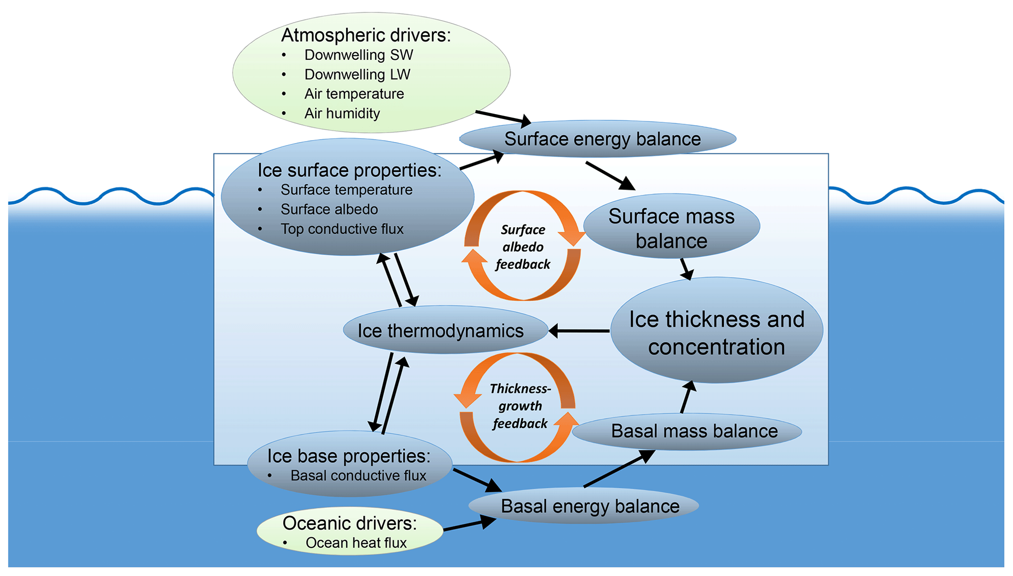
Figure 1Schematic demonstrating the causal links between the ice thickness and extent and the mass balance at the top and basal surfaces of the sea ice.
Large-scale evaluation of ice mass balance, ice thermodynamics and energy balance at the lower surface of the ice has not to date been performed for any model. This is largely because these quantities cannot yet be measured remotely but must instead be measured in situ using systems of instruments frozen into the ice. In particular, a device called an ice mass balance buoy (IMB) measures the mass balance at the upper and lower surfaces of the snow–ice column and the temperature profiles within the ice, at simultaneous locations (Perovich and Richter-Menge, 2006). Data from individual IMBs have been used to estimate sea ice energy fluxes such as conduction and ocean heat flux in the past (e.g. Perovich and Elder, 2002; Lei et al., 2014, 2018). However, IMB data have not yet been used to directly evaluate a climate model, due to the large disparity in the relevant spatial and temporal scales.
In this study, we use data from the whole IMB network to perform a large-scale evaluation of sea ice mass balance and thermodynamics in a coupled climate model. Monthly mean fluxes of top melt, top conduction, basal conduction and ocean heat flux are calculated from temperature and elevation data obtained from 104 IMBs released between 1993 and 2015; the resulting observational dataset and the code used in its production are published alongside this study, with references given in the Code availability and Data availability sections below. This dataset is then used to evaluate the sea ice in a coupled climate model (HadGEM2-ES, part of the CMIP5 ensemble) in two densely sampled regions of the Arctic, the North Pole and the Beaufort Sea. Modelled and IMB-measured fluxes are restricted to each region in turn: distributions of fluxes in each month are compared and likely model biases identified. The results of the IMB-based evaluation are compared with a previous evaluation of the sea ice state and surface radiation in the same model (West et al., 2019): the results are found both to be consistent with the results of this study and to enhance understanding of the first evaluation.
The paper is structured as follows. In Sect. 2, the IMB data and the process by which vertical energy fluxes are calculated from the data are described. In Sect. 3, the IMB flux dataset is described; seasonal, spatial and interannual variability is discussed, and uncertainty in the IMB fluxes due to various parameters used in the analysis is examined. In Sect. 4, the data are used to evaluate HadGEM2-ES, and the results are interpreted in the context of West et al. (2019). In Sect. 5, the representativity of the IMB fluxes is discussed. In Sect. 6, conclusions are presented.
The ice mass balance buoy (IMB; Perovich and Richter-Menge, 2006) network is a system of instruments frozen into a sea ice floe, allowing the simultaneous measurement of surface and base elevation, internal ice temperature (usually at 10 cm resolution), and position; many also measure surface air pressure and temperature. A diagram of an IMB is shown in Fig. 2. An IMB provides, by design, measurements of sea ice thickness and surface and basal mass balance, via the measurements of surface and base elevation. Fluxes of conduction can also be estimated from the ice temperature data (e.g. Perovich and Elder, 2002), although uncertainty is considerable due to lack of knowledge of ice salinity. In particular, the thermodynamics and basal elevation measurements can be combined to estimate ocean heat flux (Lei et al., 2014).
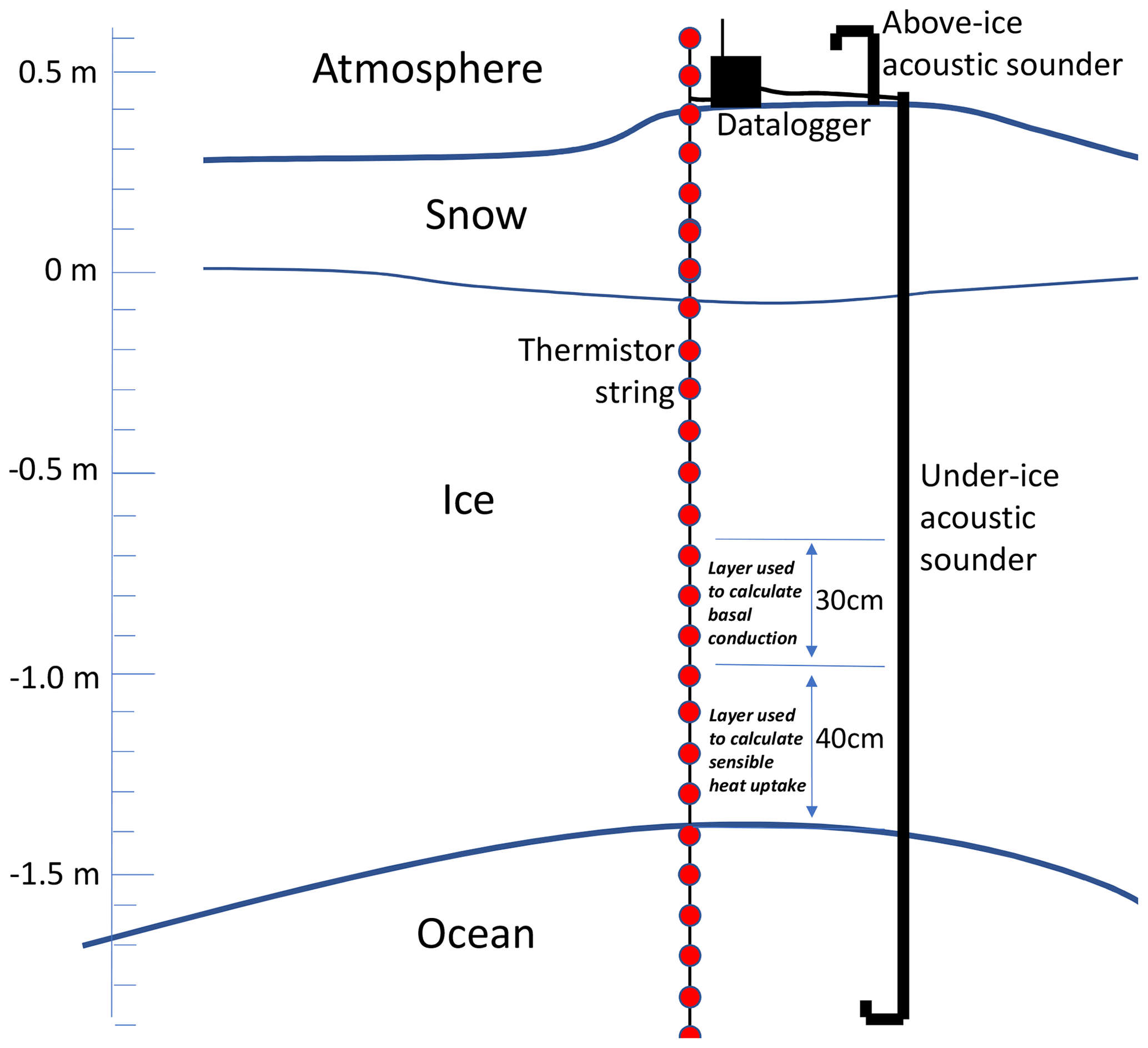
Figure 2Diagram of the main components of an IMB, with layers used in this study for calculation of fluxes at the base of the ice indicated. Adapted from Fig. 1a of Planck et al. (2019).
Data from the 104 IMBs deployed by the Cold Regions Research and Engineering Laboratory (CRREL) are stored in a series of comma-delimited CSV (comma-separated value) files at http://imb-crrel-dartmouth.org/results/ (last access: April 2020) (Perovich et al., 2020). The buoys were deployed between 1993 and 2017; spatial coverage is mainly in the North Pole and Beaufort Sea regions (Fig. 3). The buoys are identified by the year of deployment followed by a letter, for example “2012L”. Buoy lifetimes range from 4 d (2015C) to 20 months (2006C), with an interquartile range of 4–11 months. All buoys report time series of ice base elevation, snow and/or ice surface elevation, latitude, and longitude, as well as a collection of ice temperature time series taken at a number of vertical positions above, within and below the ice. In general, temperature profiles are reported at very high temporal resolution, hourly or bi-hourly, and tend to be noisy, with much high-frequency variability. From 2006 onwards, elevation data are reported at similarly high resolution but before 2006 are reported much less frequently, with intervals of a week or more between measurements.
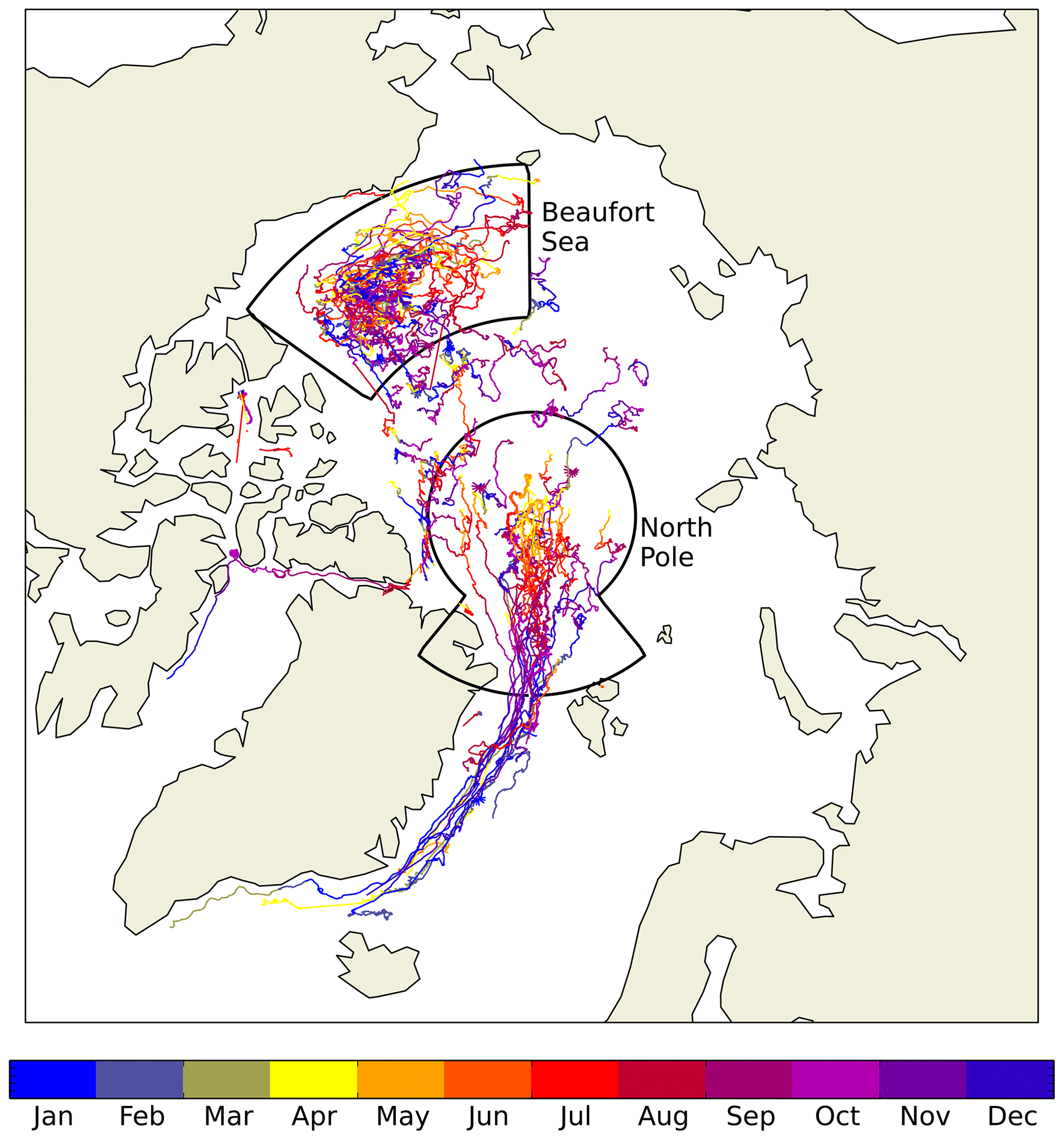
Figure 3The tracks of Arctic ice mass balance buoys from 1993 to 2015, with months of coverage indicated by the coloured shading. The North Pole and Beaufort Sea regions used in the analysis are shown by the thin black lines.
As most analysis of the data depends on the ability to perform arithmetic operations on different series, it was necessary to produce data series at consistent points in time for each buoy. To this end, modified elevation data series were produced at times coincident with the temperature measurements, using either interpolation (where there were fewer than three measurements in the 2 d period centred on the time in question) or a binomially weighted mean (where there were three or more measurements in this period). This regularization process is illustrated in Fig. 4. Although a more advanced optimal interpolation scheme would likely produce more accurate time series, inspection of individual data series shows that the current scheme produces data that are sufficiently realistic for the purposes of this study. For example, linear interpolation produces unrealistic sharp changes in the time derivative of elevation, but the effect of these on monthly mean elevation change, the derived variable used in this study, is likely to be very small.
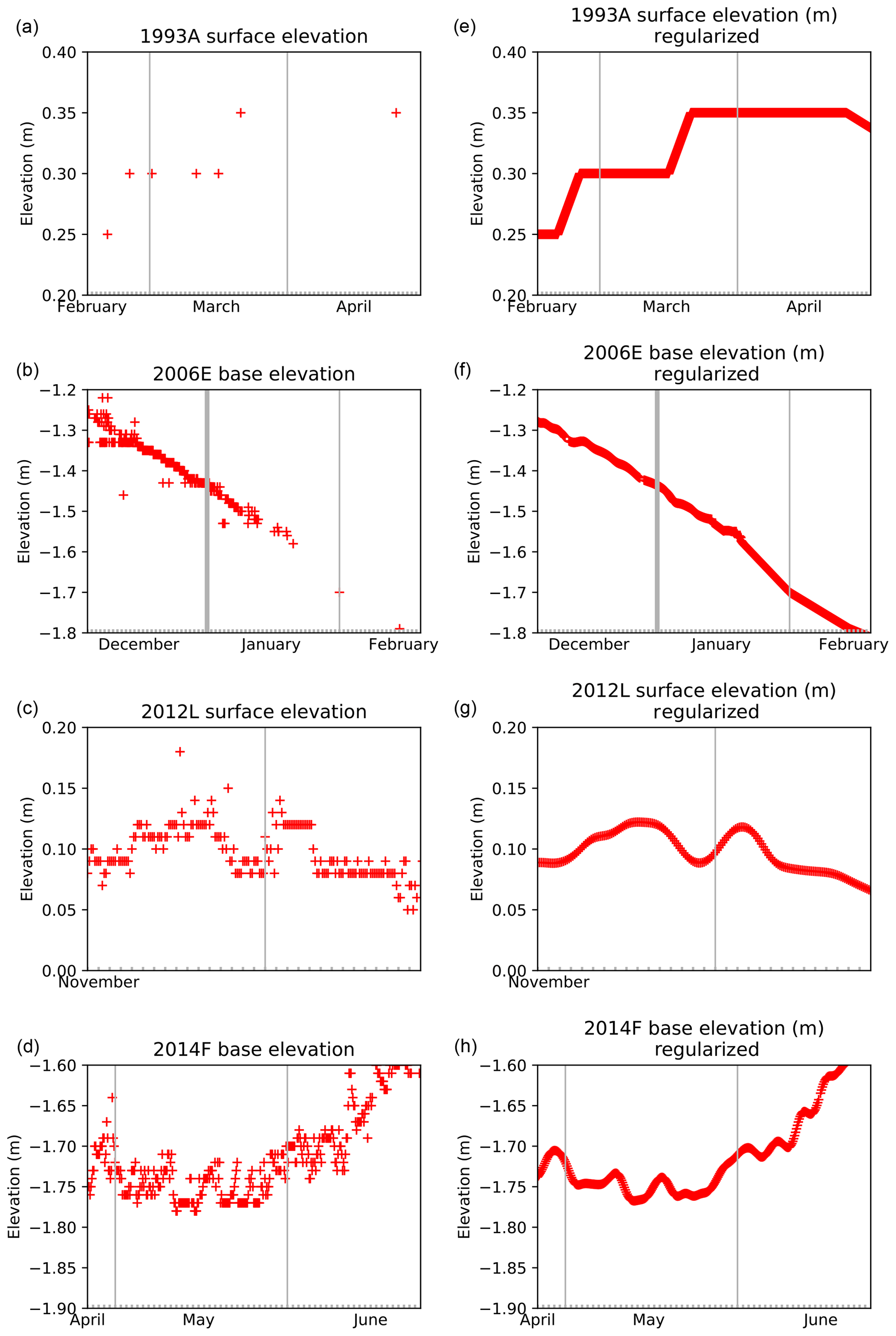
Figure 4Illustration of the regularization process using four selected IMB data series. (a, b, c, d) Raw data; (e, f, g, h) time series regularized to temperature measurement points.
The set of elevation measurements provided also varies between buoys, necessitating some processing before full regular time series of surface elevation, snow thickness, interface elevation, ice thickness and base elevation can be obtained. Some later buoys do not report surface elevation directly but report snow–ice interface elevation and snow depth, which must be summed to obtain the surface elevation. A more difficult problem is presented by the earlier buoys, which tend to produce data of surface and base elevation only. Snow–ice interface elevation must therefore be deduced from surface and base elevation, by a process illustrated in Fig. 5. Iterating through the times of observation , the interface elevation zint(t1)=0 m by construction, as the thermistor string is always referenced to the snow–ice interface at the time of deployment. At time ti, if , where zsfc(ti) represents surface elevation of the snow–ice column, we set ; but if , we set zint(ti)=zsfc(ti). In this way, the interface elevation changes only when top melting of ice is detected, i.e. when the surface elevation is judged to fall below the interface elevation estimated for the previous time of observation.
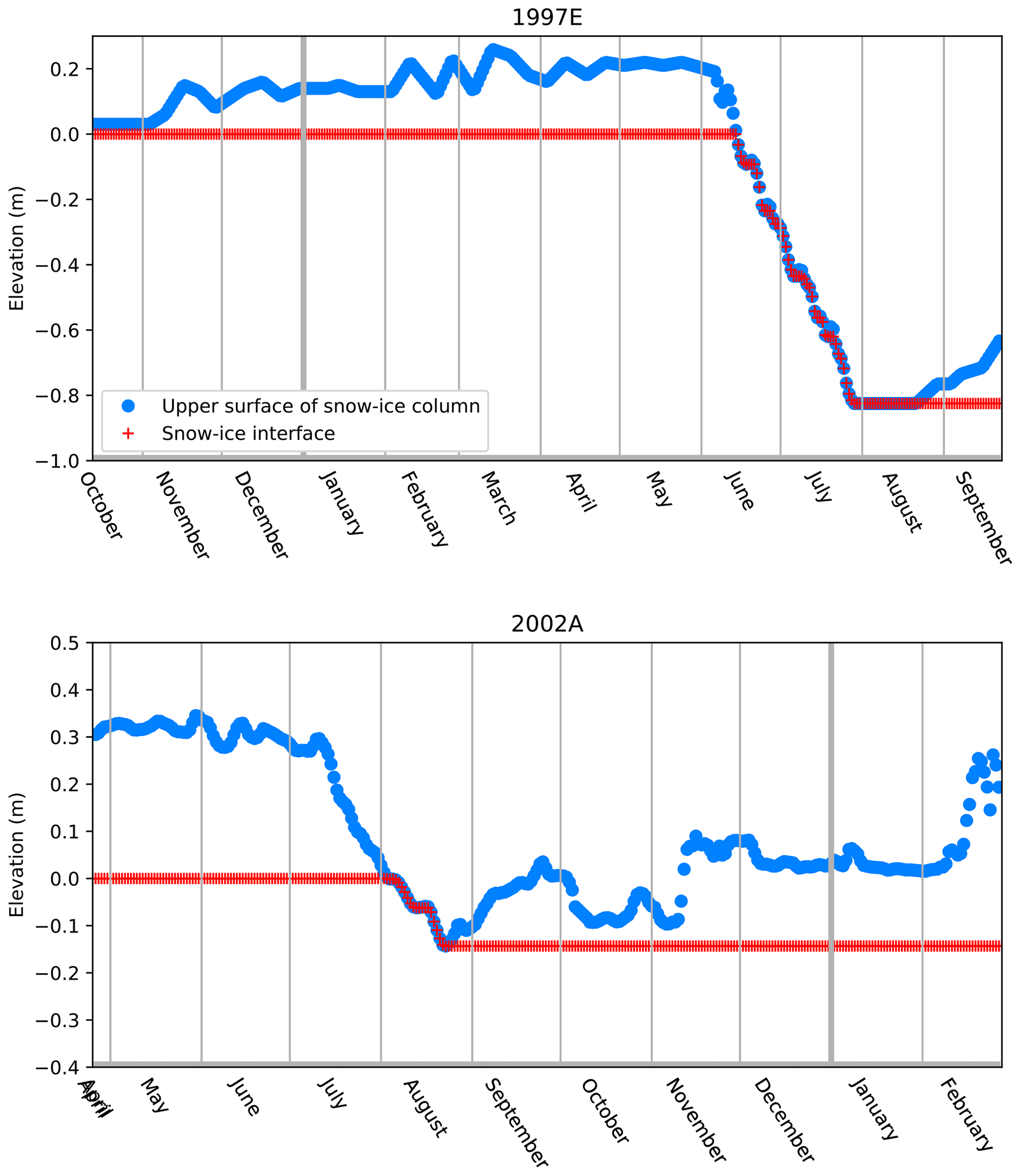
Figure 5Two examples of estimating snow–ice interface from a regularized snow surface data series. The interface remains at a constant level unless the surface falls below this level, in which case the interface falls with the surface.
This method would fail in the presence of ice flooding and snow–ice formation (e.g. as documented by Provost et al., 2017). However, while snow–ice formation is known to occur in some areas sampled by the IMBs (particularly in the North Pole region, e.g. Rösel et al., 2018), it is almost certainly a rare event in the IMB dataset. This is because the snow layer is almost always sufficiently thin relative to the ice layer that snow–ice formation is unlikely from hydrostatic principles. There are four instances when snow depth becomes sufficiently large that snow–ice formation is a possibility, but these are always associated with failure of other sensors, such that the associated data do not reach the final dataset produced in this study.
Processing the temperature data is also necessary. Instances of air, ice or ocean temperature data that are obviously wrong occur very frequently, usually characterized by sudden step changes in the temperature measurements at single – or multiple – layers that are inconsistent with simultaneous measurements in other layers, often to physically unrealistic values. The incorrect values can be caused by failure of the sensors or the datalogger or by an inability to communicate data to the receiving satellite (Donald K. Perovich, personal communication, 2019). In most cases, wrong values occurred in large groups that were difficult to identify with automatic data processing and, therefore, had to be identified by inspection and removed. From the processed temperature and elevation data, monthly mean fluxes of top melt, top conduction, basal conduction and ocean heat flux were produced in the following way. Throughout this study, the sign convention is that a positive value denotes a downwards flux and vice versa.
Top melting of ice and/or snow. This flux, commonly reported by models, represents the total energy gain by sea ice (snow) in a grid cell over the course of a month associated with melting of ice (snow) at the upper surface. It is estimated from the IMBs using the surface elevation series. A change between two adjacent daily data points in surface elevation is judged due to top melting if and only if the change is negative and the surface temperature is above a threshold value (−2 ∘C). The energy gain associated with the melting is calculated by multiplying the elevation change by ice or snow density, depending on whether the snow depth is nonzero, and by specific latent heat of fusion of ice (all parameters are defined below). The daily top melt estimates are then averaged to obtain monthly mean top melt.
Top conductive flux. This flux is defined as the conduction from the snow and/or ice surface into the ice interior. In this study it is calculated using temperatures in the top 50 cm of the snow–ice column. Where this layer lies entirely within snow (ice) the conductive flux is calculated as the temperature gradient across the layer, determined by a linear fit, by snow (ice) conductivity: values of snow and ice conductivity used are defined below.
In many cases, however, the top 50 cm is located partly within snow and partly within ice. Because snow conductivity tends to be much lower than ice conductivity, the snow–ice interface is usually associated with a sharp change in gradient that renders a linear fit meaningless. In these cases, the top conductive flux is determined by a linear fit through the same layer, using an “adjusted” temperature profile:
where zint is the elevation of the snow–ice interface, Tint−ref is temperature 5 cm below the interface, and μ=kice/ksnow – where kice and ksnow are ice and snow conductivity respectively. Physically, Tadj represents the temperature profile that the snow–ice column would have if the snow was converted to ice, Tint−ref remained the same and the vertical conductive fluxes remained the same. The effect of the adjustment is to “straighten” the profile by rotating the profile section located in the snow about Tint−ref, by a factor determined by the ratio of conductivities μ. A linear fit is then taken through a layer 0–50 cm below the snow surface and multiplied by kice to produce estimates of instantaneous top conductive flux. These are then averaged to obtain monthly means. The process is illustrated in Fig. 6.
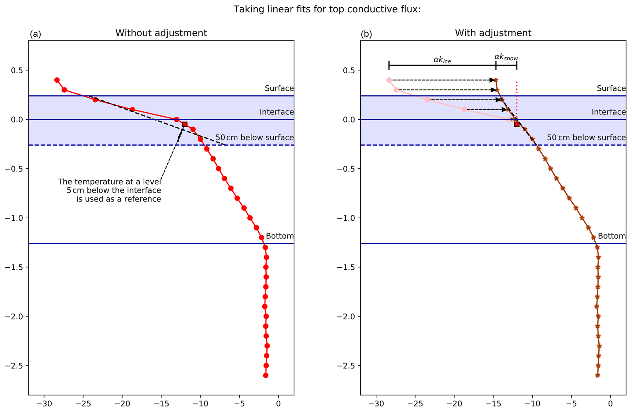
Figure 6Illustrating the process of estimating conductive flux across the top 50 cm of the snow–ice column, in the case that the snow–ice interface lies within this layer. Panel (a) shows the raw temperature profile; taking a linear fit through these points does not produce a meaningful result because of the sharp “corner” associated with the change in medium. Panel (b) shows the adjusted temperature profile; the temperatures that would be expected if the snow layer were ice, temperature below the interface and conductive fluxes remaining the same. The adjusted profile eliminates the corner, and a linear fit can be taken. In panel (b), kice denotes ice conductivity, ksnow snow conductivity and α an arbitrary constant of proportionality.
Basal conductive flux. This flux is defined as the conduction from the ice base into the ice interior. As an important component of the energy balance at the ice base, it has frequently been estimated from individual buoys in ocean heat flux calculations. Typically, temperature gradients at the ice base are small due to higher salinities here (e.g. Schwarzacher, 1959), with correspondingly higher heat capacities and lower conductivities; hence previous studies have commonly used a reference layer of a fixed thickness above which the basal conduction is estimated. In this study we use the approach of Lei et al. (2014) and calculate the basal conduction by taking temperature gradients across a layer 40–70 cm above the ice base, illustrated in Fig. 2. In Sect. 3.3 we examine the sensitivity of the derived fluxes to changes in the elevation of this reference layer, amongst other parameters. As above, the instantaneous values were averaged to a monthly mean.
Ocean heat flux. This flux is defined as the diffusive heat flux arriving at the ice base from the ocean beneath. In theory, it can be calculated as the residual of the basal conductive flux and the latent heat of melting and/or freezing at the ice base. However, using the basal conductive flux as defined above it is necessary also to take into account the sensible heat uptake of the intervening layer (the “buffer zone”), 0–40 cm above the ice base, illustrated in Fig. 2. The ocean heat flux can then be written as
as in Lei et al. (2014).
The basal conductive flux Fcondbot is defined as above. Monthly mean Fsens, the sensible heat flux in the 0–40 cm layer, is calculated as the average of daily heat uptake rates obtained by taking linear fits through all temperature points within 1 d of a given time instant for all vertical points in this layer, summing these (weighted according to layer thickness) and multiplying by ice density and heat capacity, defined below. Finally, monthly mean latent heat of melting at the ice base, Flat, is calculated from the base elevation time series, by multiplying daily differences in elevation by specific latent heat of fusion.
The calculation of thermodynamic parameters is now described. In this study, we take the approach of using a “standard” set of thermodynamic parameters to calculate the main dataset of energy fluxes, demonstrated in Sect. 3.1 and 3.2 below, and subsequently evaluate sensitivity to the values of these parameters in Sect. 3.3. Ice density ρice, snow density ρsnow and latent heat of melting qfus are set to 917 kg m−2, 330kg m−2 and 3.34×10⁵ J kg−1 respectively, the standard values used by the sea ice model CICE (Hunke et al., 2013).
Ice conductivity is defined after Maykut and Untersteiner (1971) as
where S and T are ice salinity and temperature respectively, kfresh=2.03 W m−1 K−1, the conductivity of fresh ice, and β=0.13 W m−1 is an empirically determined constant representing the effect of brine pockets on conductivity. For the calculation of the top conductive flux, a practical salinity of 1.0 is used, while the temperature used is that of the snow–ice interface. For the calculation of the basal conductive flux, a practical salinity of 4.0 is used, multiplied by the mean value of 1/T, where the average is taken over the time period in question and the layer 40–70 cm above the ice base.
Specific heat capacity is defined after Ono (1967) as
where cfresh=2106 J kg−1 K−1 is the specific heat capacity of fresh ice, J kg−1 the specific latent heat of fusion of fresh ice, and μ=0.054 K the ratio between water salinity and freezing temperature. In calculating sensible heat uptake at the ice base, again a practical salinity of 4.0 is used, multiplied by the mean value of 1/T2, where the average is taken over the time period in question and the layer 0–40 cm above the ice base.
Ice salinity must also be taken into account when calculating latent heat of freezing and melting. The energy required to melt a given volume of sea ice at temperature T, from Bitz and Lipscomb (1999) is
At the lower surface of the ice, q is calculated by setting ∘C and S=4.0 as above. At the upper surface of the ice, T is usually extremely close to 0 ∘C when melting is taking place, meaning that a choice of S that is both consistent and physically realistic in all cases is difficult to make. Instead, it is assumed that the ice at the upper surface is fresh and q=qfresh is used.
The monthly heat fluxes calculated above are subject to several sources of uncertainty. These are evaluated in detail in Sect. 3.3 below, but the issues are briefly summarized here. Firstly, there is significant uncertainty due to lack of knowledge of ice salinity, which affects the fluxes through the ice conductivity and heat capacity. Secondly, the manner of dependence of ice conductivity on salinity is also subject to uncertainty, with an alternative formulation to Maykut and Untersteiner being proposed by Pringle (2007). Thirdly, both snow and ice density are subject to uncertainty, affecting the diagnosis of melting and freezing fluxes at the top and basal surfaces of the ice from elevation changes (as well as sensible heat uptake in the lowest layer of the ice). Finally, the reference layers chosen to evaluate conductive and heat uptake fluxes are themselves a parameter of the analysis and as such represent an additional source of uncertainty.
Examination of the monthly mean energy fluxes reveals several ways in which unrealistic estimates might be produced. Firstly, in a small minority of months, top or basal ice temperature is warmer than the melting point associated with the assumed salinity (1 at the top of the ice and 4 at the base), resulting in the conduction or sensible heat uptake being very large or undefined. For these months, the salinity is set instead to the highest physically allowable value, given the maximum temperature attained.
A second problem relates to the formation of false bottoms under sea ice, as documented by Notz (2003), in which meltwater refreezes upon meeting cold seawater at a temperature below its own melting point. This process visibly occurs during the period of operation of some buoys (for example 2015A, demonstrated in Fig. S1 in the Supplement), associated with sudden step changes in base elevation. These result in very large negative monthly mean ocean heat fluxes being calculated during the month of formation and correspondingly large positive fluxes during the month of dissipation. These fluxes are physically unrealistic, as the large changes in elevation usually represent the freezing and melting of only a very thin layer of ice, with liquid seawater remaining in between this layer and the main body of the ice column. In some cases, it may be possible to estimate true ocean-to-ice heat flux simply by interpolating base elevation between the apparent times of formation and dissipation, but this approach is likely to be inaccurate for long-lived false bottoms. For the purposes of this study all affected ocean heat fluxes were simply removed from the dataset, as they were relatively few in number.
3.1 Seasonal and spatial variability
Throughout the description of the IMB-estimated fluxes here – and the model evaluation below – the convention used is that positive numbers denote downwards fluxes and vice versa. The distributions of monthly mean fluxes of top melting, top conduction, basal conduction and ocean heat flux are summarized in Table 1. The IMBs provide 463 monthly mean values of top melt in total, ranging from 31 values in March and August to 53 in May. The seasonal cycle reaches its maximum in July, when top melting of 29.9±17.8 W m−2 is observed. Strong top melting is also evident in June (16.8±11.0 W m−2), but top melting tends to be considerably lower in August (8.1±6.7 W m−2). In all 3 summer months, the distribution is positively skewed, with a small number of very high values (for example, the highest top melt value recorded is 79.9 W m−2, for buoy 1993A in July 1993). Values for the rest of the year are zero or near zero. Throughout the year, standard deviation of the distributions is of a similar order of magnitude to the mean, showing a high degree of spatial and interannual variability.
Table 1Mean and standard deviations of fluxes measured from the IMB data (in W m−2), in each month of the year. For each flux, the convention is that downwards indicates positive.
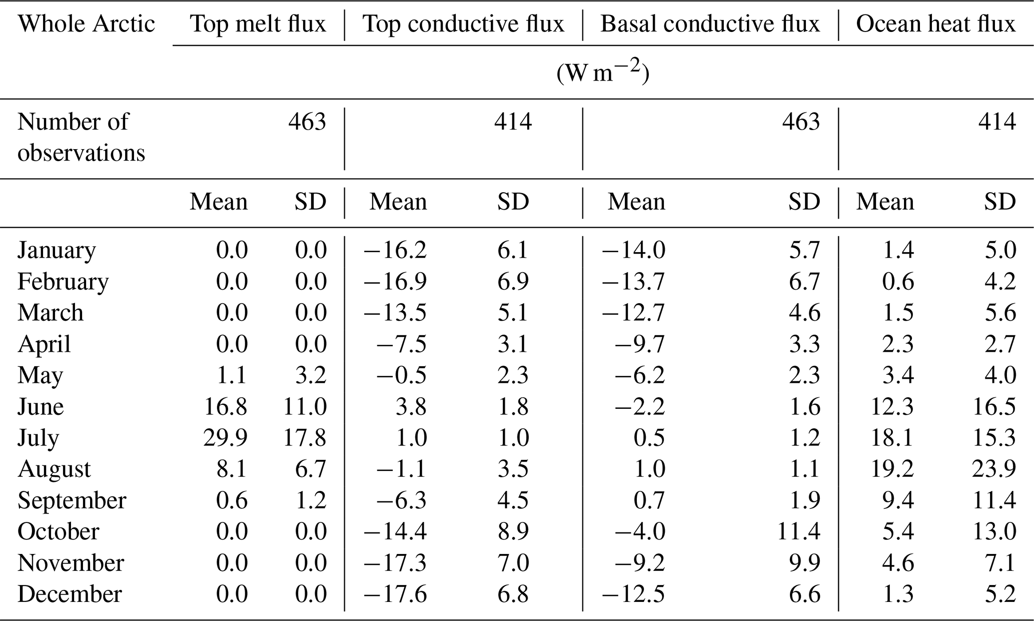
Top conductive flux, a component of the surface energy balance, is the means by which the ice loses energy to the atmosphere in the presence of atmospheric cooling during the Arctic winter. It depends not only strongly upon atmospheric conditions but also upon ice and snow thickness, as thinner ice and snow can support stronger temperature gradients and conduct energy upwards more quickly. For the top conductive fluxes, the IMBs provide 414 estimates in total, ranging from 24 in August to 51 in May. Mean top conductive fluxes are strongly negative from October to March, reaching a minimum value of W m−2 in December. However, values are weakly positive in June and July, reflecting warming of the ice interior.
The basal conductive flux acts to remove energy from the ice base in winter, allowing ice growth, and to a lesser extent during late spring and early summer while the ice is warming, attenuating ice melt. For the basal conductive fluxes the IMBs provide 463 estimates, ranging from 29 in August to 52 in May. The basal conductive flux displays a seasonal cycle less amplified than – and displaced slightly later relative to – that of the top conductive flux, with lowest values occurring from November to April and a minimum of W m−2 occurring in January. The damped response relative to the top conductive flux occurs due to the thermal inertia of sea ice and the principal thermodynamic forcing occurring at the top surface.
Lastly, for the ocean heat fluxes, the IMBs provide 414 estimates, ranging from 25 in August to 49 in May. The highest values are seen in July and August, with a mean and spread of 18.1±15.3 and 19.2±23.9 W m−2 respectively. The distributions in these months are, like the top melting flux, strongly positively skewed, with a small number of exceptionally high values. Notably, 119 W m−2 is estimated in August 2007 for buoy 2006C in the Beaufort Sea, as part of a summer of extreme ice melt documented by Perovich et al. (2008). In the winter, mean values of ocean heat flux are near zero. There is frequent occurrence of small negative estimates in the distributions in the winter. These are likely to be spurious and reflect errors in assumptions made about the salinity and density at the base of the ice. For most such values, the uncertainty interval resulting from varying the salinity from 0 to 10 encompasses 0 W m−2.
Two regions of the Arctic are relatively densely sampled by the IMBs: the Beaufort Sea and the North Pole (Fig. 3). In order to demonstrate that the IMBs are able to capture some regional variability, especially to aid with model evaluation in Sect. 4 below, monthly mean fluxes derived from buoy tracks entirely within these regions were sorted into separate datasets, characteristics of which are now described separately. Mean and standard deviations of the distributions in the North Pole and Beaufort Sea regions are summarized in Tables 2 and 3 respectively; boxplots are presented in Fig. 7. Significance of differences between distributions is measured using a Welch t test, with a 5 % p-value threshold.
Table 2Means and standard deviations of fluxes measured from the IMB data in the North Pole region (in W m−2), in each month of the year. For each flux, the convention is that downwards is positive.
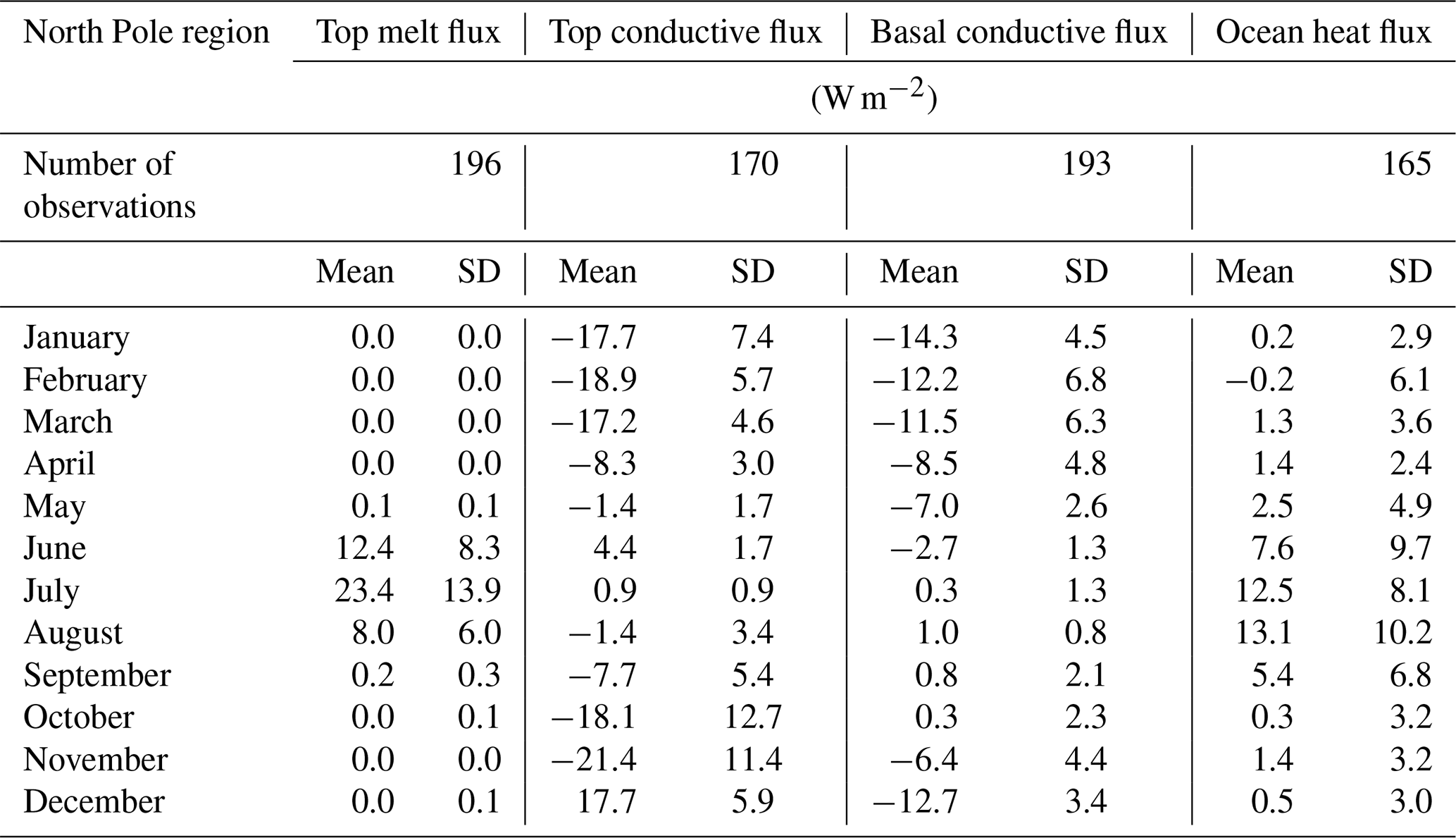
Table 3Means and standard deviations of fluxes measured from the IMB data in the Beaufort Sea region (in W m−2), in each month of the year. For each flux, the convention is that downwards is positive.
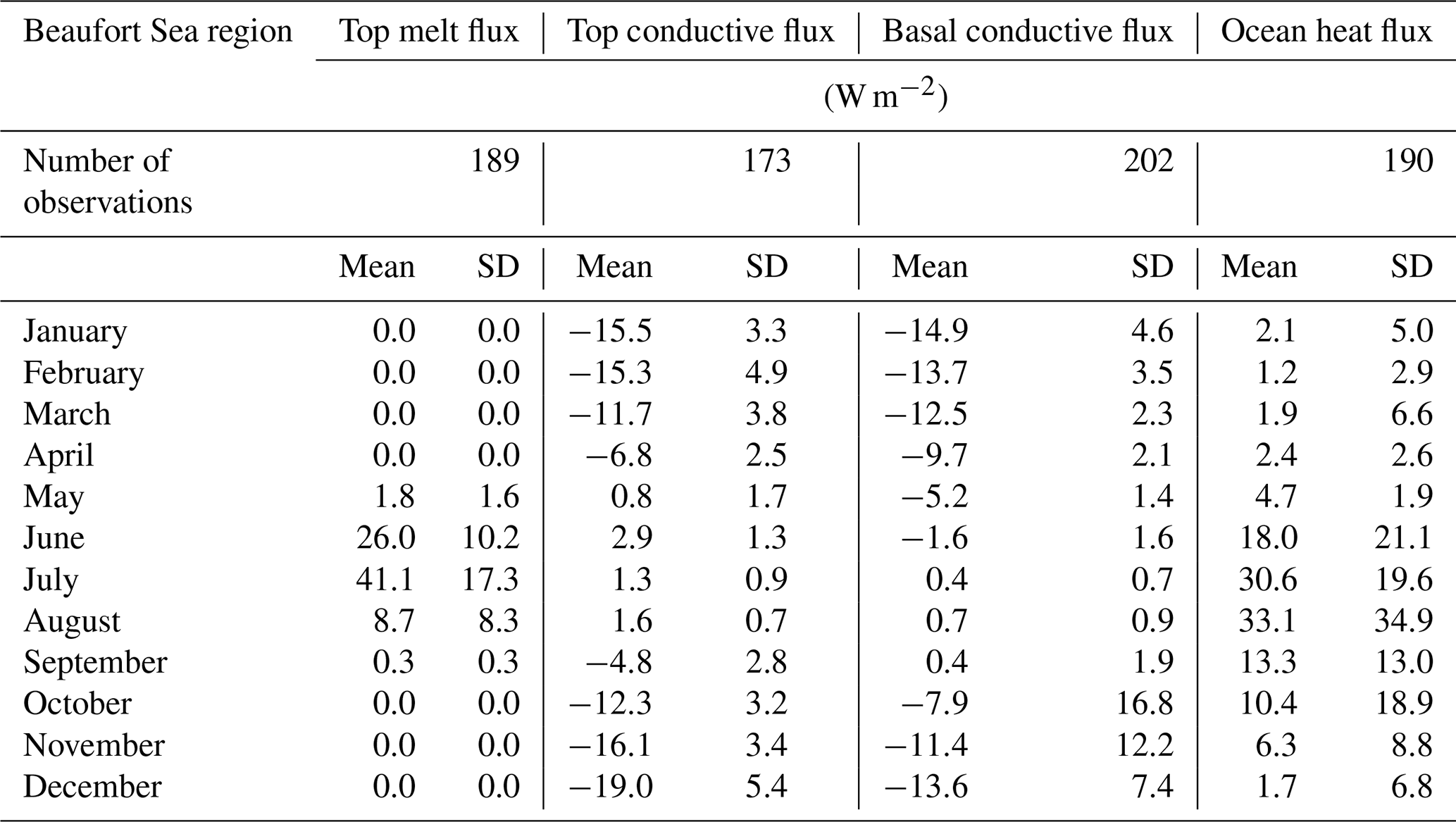
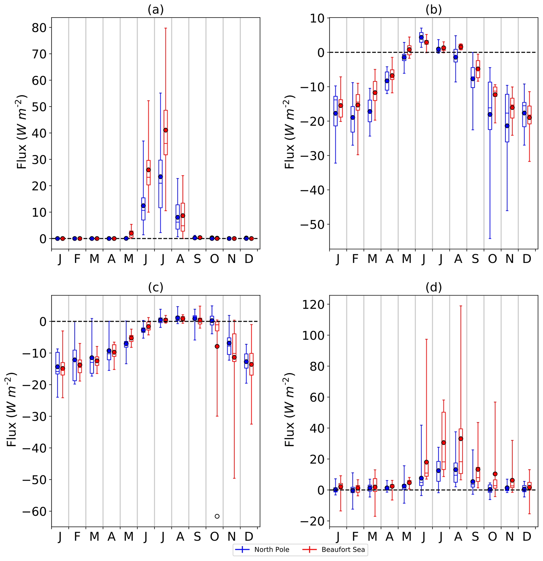
Figure 7Fluxes of (a) top melting, (b) top conductive flux, (c) basal conductive flux and (d) ocean heat flux, estimated from the IMB data, shown for North Pole (blue) and Beaufort Sea (red) regions. For each month, flux and region, the distribution is indicated by a boxplot showing range, interquartile range, median (horizontal lines) and mean (filled circles). For all fluxes, the convention is that downwards is positive.
Top melting fluxes are shown in Fig. 7a separately for the Beaufort Sea and the North Pole regions. In June, the top melting fluxes measured in the North Pole region range from 1 to 37 W m−2, with a mean of 12±8 W m−2, while those measured in the Beaufort Sea range from 10 to 52 W m−2 with a mean of 26±10 W m−2. The lower distribution in the North Pole region is consistent with the observed later onset of surface melting here (Markus et al., 2009) associated with the higher latitude. In July, measured fluxes range from 2 to 55 W m−2 in the North Pole region, with a mean of 23±14 W m−2, and 11 to 80 W m−2 in the Beaufort Sea region, with a mean of 41±17 W m−2. In both June and July, distributions of top melt fluxes are significantly different in the two regions. Measured fluxes of top melting are much lower in August in both regions.
For the top conductive flux (Fig. 7b), winter fluxes tend to be slightly higher in magnitude in the North Pole than in the Beaufort Sea region, although in no winter months are the distributions significantly different at the 5 % level. In January, for example, North Pole fluxes range from −32 to −10 W m−2 with a mean of W m−2, while those in the Beaufort Sea region range from −20 to −7 W m−2 with a mean of W m−2. Some notable differences between the distributions occur in the “shoulder seasons”, particularly in May and August (when the distributions are significantly different), with higher values, indicating ice warming, occurring in the Beaufort Sea region. For example, in May, values in the North Pole region range from −6 to 3 W m−2 with a mean of W m−2, while values in the Beaufort Sea region range from −2 to 4 W m−2 with a mean of 1±2 W m−2. These differences indicate earlier onset of warming in the Beaufort Sea and earlier onset of cooling in the North Pole region, consistent with an earlier onset of surface melt in the Beaufort Sea.
Less spatial variability is evident for the mean basal conductive flux (Fig. 7c). For example, in December, North Pole fluxes range from −20 to −7 W m−2 with a mean of W m−2, while Beaufort Sea fluxes range from −32 to −1 W m−2 with a mean of W m−2. Hence the thermal inertia of ice appears to have some damping effect on the larger variability in thermal forcing evident in the Beaufort Sea region from the top conductive flux. Winter variability tends to be higher in the Beaufort Sea than the North Pole, but this is largely caused by a small number of exceptionally low fluxes early in the winter associated with end-of-summer ice thicknesses of 50 cm or lower, notably a value of −61.7 W m−2 recorded in October 2007 for buoy 2006C. The faster warming and slower cooling of ice evident in the shoulder seasons in the Beaufort Sea region for the top conductive flux are also not evident for the basal conductive flux. In the month of May, for example, basal conductive flux values range from −13 to 0 W m−2 in the North Pole region with a mean of W m−2, compared to a range of −8 to −2 W m−2 and mean of W m−2 in the Beaufort Sea region.
For the ocean heat flux (Fig. 7d), in the summer very high values tend to be more common in the Beaufort Sea region than in the North Pole region. For example, in August, North Pole region values range from 2 to 38 W m−2 with a mean of 13±10 W m−2, while the Beaufort Sea region values range from 7 to 119 W m−2 with a mean of 33±35 W m−2. It is likely that these are related to the lower ice fractions and greater solar heating of the mixed layer in the Beaufort Sea region.
3.2 Interannual variability
Having examined spatial and seasonal variability in the estimated fluxes, it is natural to consider whether the dataset also gives useful information about interannual variability. Restricting fluxes to individual years does not give enough data points (per month) to permit analysis, particularly early in the period where very often there was only one or two buoys in operation in any particular year (and in some cases none). Instead, the period of the IMB operations is divided into three sections with very roughly equal numbers of data points for each flux and month: 1993–2006, 2007–2012 and 2013–2015. The middle period is chosen to contain the 2 years with the lowest September extents (2007 and 2012, according to HadISST1.2, Hadley Centre Sea Ice and Sea Surface Temperature data set, version 1.2) in the entire analysis period, to maximize the chance that interannual variability can be detected. For each flux and month of year, we compare the distribution of values estimated for each period (Fig. 8) and use a Welch t test to judge whether any distributions are significantly different at the 5 % level.
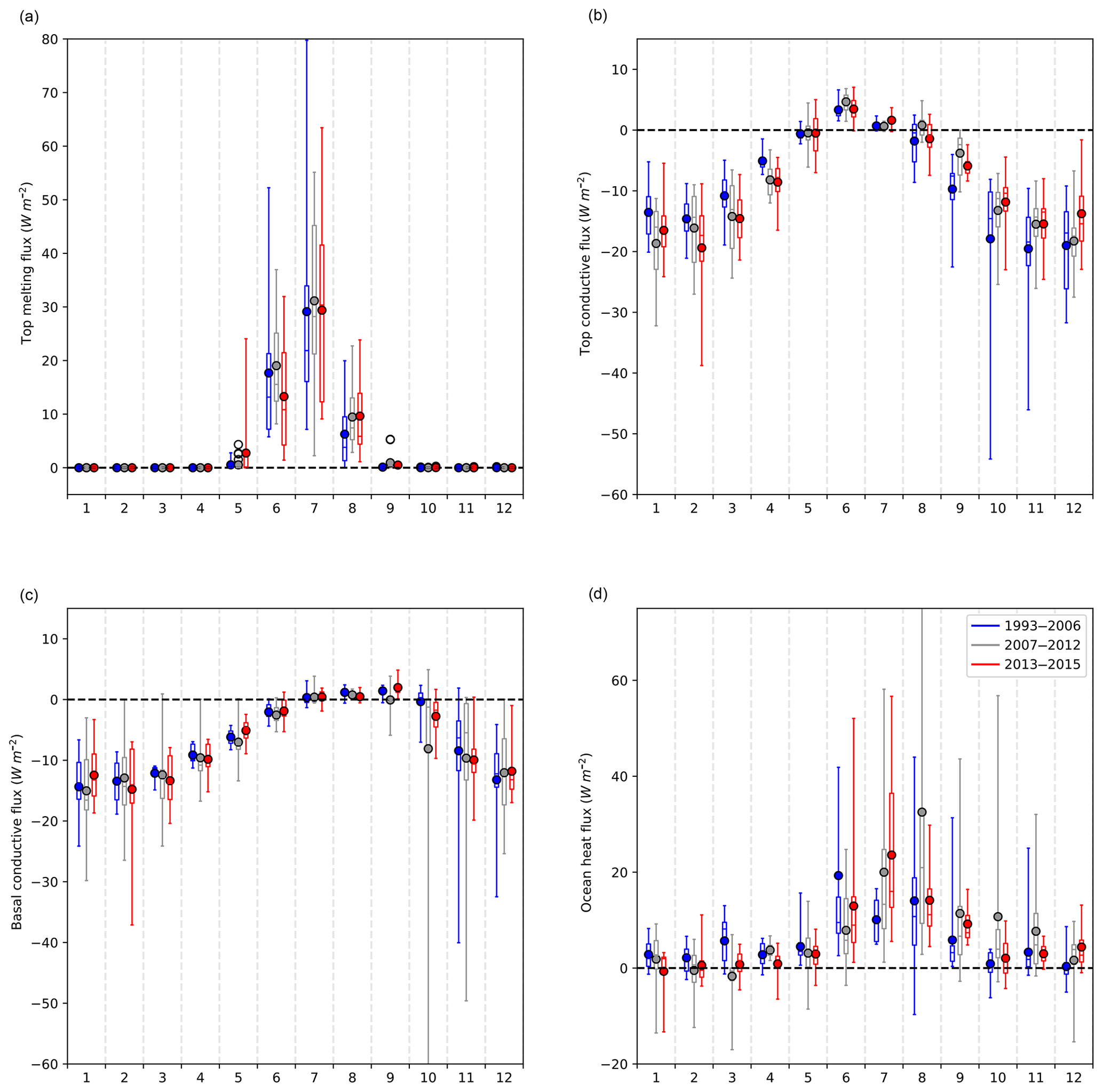
Figure 8IMB-measured distributions of (a) top melting; (b) top conductive flux; (c) basal conductive flux, and (d) ocean heat flux, divided into the three periods 1993–2006, 2007–2012, and 2013–2015. Each distribution is illustrated with a boxplot showing range, interquartile range, median (horizontal lines) and mean (filled circles).
For the top melting flux, in no months are the distributions significantly different, and in July and August means and standard deviations are very similar. In May, however, the mean top melting flux is higher in the later period 2013–2015 (2.7±5.8 W m−2) than in the middle (0.5±1.0 W m−2) and early (0.5±0.9 W m−2) periods. By contrast, in June the mean top melting flux is lower in the later period (13.3±9.6 W m−2) than in the middle (19.0±8.8 W m−2) and early (13.7 W m−2) periods. The differences could conceivably reflect the observed trend towards earlier onset of melt (e.g. Bliss et al., 2019), but the lack of significance makes drawing conclusions difficult.
Early in the winter, the top conductive flux becomes higher (less negative) as time passes; for example, in October the distribution means are , and W m−2 for the periods 1993–2006, 2007–2012 and 2013–2015 respectively. Late in the winter, the trend reverses, with top conductive flux becoming lower (more negative) as time passes: for example, in March the distribution means are , , W m−2 for the three periods respectively. However, as with the top melting fluxes, the distributions are not significantly different. Differences in basal conductive flux are still less marked, with distributions similar in all months except October, where the middle period displays a much higher (more negative) mean and greater spread due to the presence of a small number of extreme values (including that from buoy 2006C, noted above).
For the ocean heat flux, an upward trend is apparent in the month of July, with means of 10.1±4.4, 20.0±17.0 and 23.6±17.1 W m−2 for the three periods respectively; for the early and late periods, the distributions are barely significantly different. In August, the mean in the middle period (32.5±37.0 W m−2) is much higher than that of the early (14.0±15.1 W m−2) and late (14.1±9.5 W m−2) periods, but the differences are not significant. The paucity of significant differences between distributions, coupled with the deliberate choice of periods to maximize interannual variability, suggests that it is difficult to detect robust interannual trends in the IMB dataset in its current state.
3.3 Uncertainty associated with assumptions of the analysis
We assess uncertainty due to ice salinity, snow and ice density, ice conductivity and the layers used to calculate conductive flux and ocean heat flux. Guided by estimates produced in the modelling studies of Turner et al. (2015) and Vancoppenolle et al. (2008), we use a practical salinity range of 0–10 to evaluate uncertainty due to salinity at both upper and basal surfaces of the ice. In fact, the ice salinity causes by far the greatest uncertainty in all measured fluxes, and the effect is most marked when considering the top melting flux. For example, the top melting flux estimated from buoy 1997D in the month of July 1998 is 31.0 W m−2 when a salinity of 0 is assumed but 0.4 W m−2 with a salinity of 10. This is due to the much lower latent heat of fusion of ice at higher salinities. Over the distribution of a whole, average July top melting flux is 29.9 W m−2 with a salinity of 0 but 1.6 W m−2 with a salinity of 10.
At first sight, the large uncertainties would render evaluation of the top melting flux in a sea ice model using IMB data extremely difficult. However, the physical meaning of this uncertainty must be correctly understood. The specific latent heat of high-salinity ice is lower because a significant fraction of the ice will already have undergone melting. The energy used in melting this ice is accounted for in sensible heating of the top layer of ice, as high -salinity ice has a higher heat capacity for this reason. In a sense, top melting of ice and sensible heating of the top layer are part of the same process. Undertaking a meaningful evaluation of modelled top melting using the IMB fluxes therefore requires consideration of the thermodynamic treatment of ice in that model. For example, in a model such as HadGEM2-ES, it is appropriate to compare modelled top melting to energy used in melting the entire top layer of ice – equivalent to assuming an ice salinity of 0 in the IMB dataset. This is because HadGEM2-ES does not model ice salinity or heat capacity (as described in more detail in Sect. 4 below).
The salinity has a much smaller, though still noticeable, effect on the conductive flux. In February 2014, for example, a salinity of 0 is associated with a top conductive flux of −12.5 W m−2, while a salinity of 10 is associated with a flux of −11.8 W m−2. Over the whole dataset, the average February top conductive flux is −17.0 (−16.6) W m−2 when a salinity of 0 (10) is assumed. Sensitivity is higher in the summer, as conductivity is more sensitive to salinity at higher temperatures: over the dataset, the average July top conductive flux is 3.1 (−0.1) W m−2 when a salinity of 0 (10) is used. The basal conductive flux displays highest sensitivity to salinity from February to April; for example, the average March basal conductive flux is −13.3 (−11.7) W m−2 when a salinity of 0 (10) is assumed.
Ocean heat fluxes tend to display higher sensitivity to salinity than do the conductive fluxes but lower than does the top melting flux. This is mainly because temperatures tend to be lower at the basal surface of the ice than at the top during the summer (when top melting and ocean heat fluxes tend to be greatest in magnitude), reducing sensitivity of the latent heat of fusion of ice to salinity. For example, in August 2003, buoy 2003D displays an ocean heat flux of 24.3 (16.6 W m−2) when salinity of 0 (10) is assumed. For the distribution as a whole, sensitivity is highest in the month of August when the mean ocean heat flux is 23.0 (13.5) W m−2 when salinity of 0 (10) is assumed.
To examine sensitivity to snow density, we use the range 274–374 kg m−3, after Alexandrov et al. (2010). Snow density only affects the top melting flux; the highest sensitivity is seen in the month of June, where the average top melting flux is 15.4 (17.9) when snow density of 274 (374) kg m−3 is used. We also examine sensitivity to ice density, using the range 917–944 kg m−3, after Cox and Weeks (1983); for the top melting flux, the highest sensitivity is in July, when the average top melting flux is 29.9 (30.7) W m−2 when ice density is 917 (944) kg m−3. The ocean heat flux also depends on ice density, and the largest difference occurs in the month of August, when the average flux is 19.9 (20.5) W m−2 when ice density is 917 (944) kg m−3.
Ice conductivity is also subject to considerable uncertainty. An alternative formulation to the Maykut and Untersteiner method used in this study was proposed by Pringle (2007) following laboratory tests of land-fast sea ice, in which sea ice conductivity kI (in W m−1 K−1) is calculated from ice temperature T (in ∘C) and practical salinity S as
Sensitivity of the IMB-measured fluxes to the conductivity formulation was tested by recalculating conductive and ocean heat fluxes using this alternative method (there is no difference in the top melting fluxes by design). Large difference in the winter top conductive fluxes are apparent, due to the Pringle (2007) formulation tending to produce much higher conductivities at low temperatures. For example, for buoy 1993A in January 1994, a top conductive flux of −18.3 W m−2 is estimated using the Pringle formulation but only −15.8 W m−2 using the Maykut and Untersteiner (1971) formulation. For the dataset as a whole, a mean January top conductive flux of −21.0 W m−2 is estimated with the Pringle formulation and −17.7 W m−2 with the Maykut and Untersteiner formulation.
Finally, sensitivity of the IMB basal conductive and ocean heat fluxes to the depth and thickness of the reference layers used was tested. The fluxes were recalculated with the lowest 20 cm of the ice used to calculate sensible heat uptake and the layer 20–40 cm above the ice base to calculate basal conductive fluxes. The largest change in mean basal conductive flux occurs in October, with a mean value of −0.7 W m−2 as opposed to −4.1 W m−2 in the standard configuration. This is associated with temperature gradients being smaller closer to the ice base. The difference decreases through the winter, with −11.7 W m−2 in February, as opposed to −13.7 W m−2 in the standard configuration. The largest difference in ocean heat flux also occurs in October, with a mean value of 2.8 W m−2 as opposed to 5.4 W m−2 in the standard configuration.
In summary, varying parameters of the analysis results in measurable changes to the IMB fluxes. In most cases, however, the sensitivity of the fluxes to the parameters is an order of magnitude lower than the absolute values, in the months of the year when the absolute values tend to be at their peak (winter for the conductive fluxes; summer for the top melting and ocean heat fluxes). The main exception is the effect of salinity on the top melting fluxes in summer, but as noted above, care is needed when interpreting this uncertainty in the context of a model evaluation.
4.1 Evaluating vertical energy fluxes in HadGEM2-ES with the IMBs
In this section, the distributions of energy fluxes estimated from the IMB data are compared to equivalent fluxes simulated by the coupled climate model HadGEM2-ES. This model, developed from the earlier model HadGEM1, is based on the HadGEM2-AO coupled atmosphere–ocean system but employs additional components to simulate terrestrial and oceanic ecosystems, in addition to tropospheric chemistry (Collins et al., 2011). The sea ice component is very similar to that used by HadGEM1 (McLaren et al., 2006), employing a subgrid-scale thickness distribution with five categories (Thorndike et al., 1975), elastic–viscous–plastic rheology (Hunke and Dukowicz, 1997) and a zero-layer thermodynamics scheme, described in the appendix to Semtner (1976), in which sea ice has no heat capacity and conduction does not vary with height within the ice. The atmosphere and ocean components contain a number of improvements relative to HadGEM1 (The HadGEM2 Development Team, 2011). The sea ice in HadGEM2-ES is modelled on a regular latitude–longitude grid, with a resolution of 1∘ throughout the Arctic.
The Arctic sea ice and surface radiation simulation of the historical ensemble of HadGEM2-ES was evaluated by West et al. (2019). A number of likely model biases were identified; a low bias in September sea ice extent, a low bias in annual mean ice thickness and a high bias in ice thickness seasonal cycle amplitude, and a tendency to model overly high surface net downwelling shortwave (SW) flux in summer and overly low surface net downwelling longwave (LW) flux in winter. To perform the evaluation of the ice energy budget in the present study, the model period 1980–1999 is used, chosen to match the period used in West et al. (2019).
For each month, grid cells lying inside the North Pole and Beaufort Sea regions (Fig. 3) are separately identified, and monthly mean top melt flux, top conductive flux, basal conductive flux and ocean heat flux are collected into distributions. Means and standard deviations of these distributions are then compared to those of the IMB fluxes, with model fluxes weighted by grid cell area when calculating these statistics. Before aggregation the fluxes, produced by the model as grid-box means, are divided by ice area to produce means over ice only, for greater consistency with the IMB fluxes. As above, to compare modelled and observed distributions in a systematic manner, a Welch t test is used, and the 5 % level is chosen as a threshold for significance of difference in distributions.
The approach of calculating model distributions over whole regions and time periods, rather than comparing only grid cells lying under IMB tracks during the respective month, is chosen for two reasons. Firstly, internal variability is such that no climate model would be expected to capture the exact atmospheric conditions over a specific IMB track; whether the model could capture the average conditions over a larger-scale region and time period is a more useful question for evaluation purposes. Secondly, even a model grid-cell implicitly models sea ice of many different thicknesses, due to the ice thickness distribution, and therefore the comparison with IMB tracks cannot be made more like-for-like by restricting to a single grid cell.
For both regions, top melt fluxes simulated by HadGEM2-ES tend to be much higher than those measured by the IMBs (Fig. 9a, b); modelled and observed distributions are significantly different throughout the melt season. For example, the modelled mean top melt flux of 72.5±8.2 W m−2 in the Beaufort Sea region in June is much higher than the IMB mean of 26.0±10.2 W m−2; in the North Pole region in June, the modelled mean top melt flux of 56.6±14.0 W m−2 is much higher than the IMB mean of 12.4±8.3 W m−2. A Welch t test shows the modelled and observed distributions of top melt fluxes to be significantly different at the 5 % level throughout the summer in both regions. The phase of the annual cycle in top melt is shifted slightly earlier, with the effect that, in both regions, the modelled June and July means are very similar, while the IMB estimates show a distinct maximum in July. However, the greater top melt in the Beaufort Sea region relative to the North Pole region is captured by the model. The bias towards excessive top melting displayed by HadGEM2-ES is consistent with the finding by West et al. (2019) that summer net SW fluxes are overestimated in HadGEM2-ES. It was shown in this study that this was likely associated with an early onset of surface melting in the model. In turn, this triggers the melt pond parameterization of HadGEM2-ES, lowering surface albedo at an earlier time of year than melt ponds would have formed in reality.
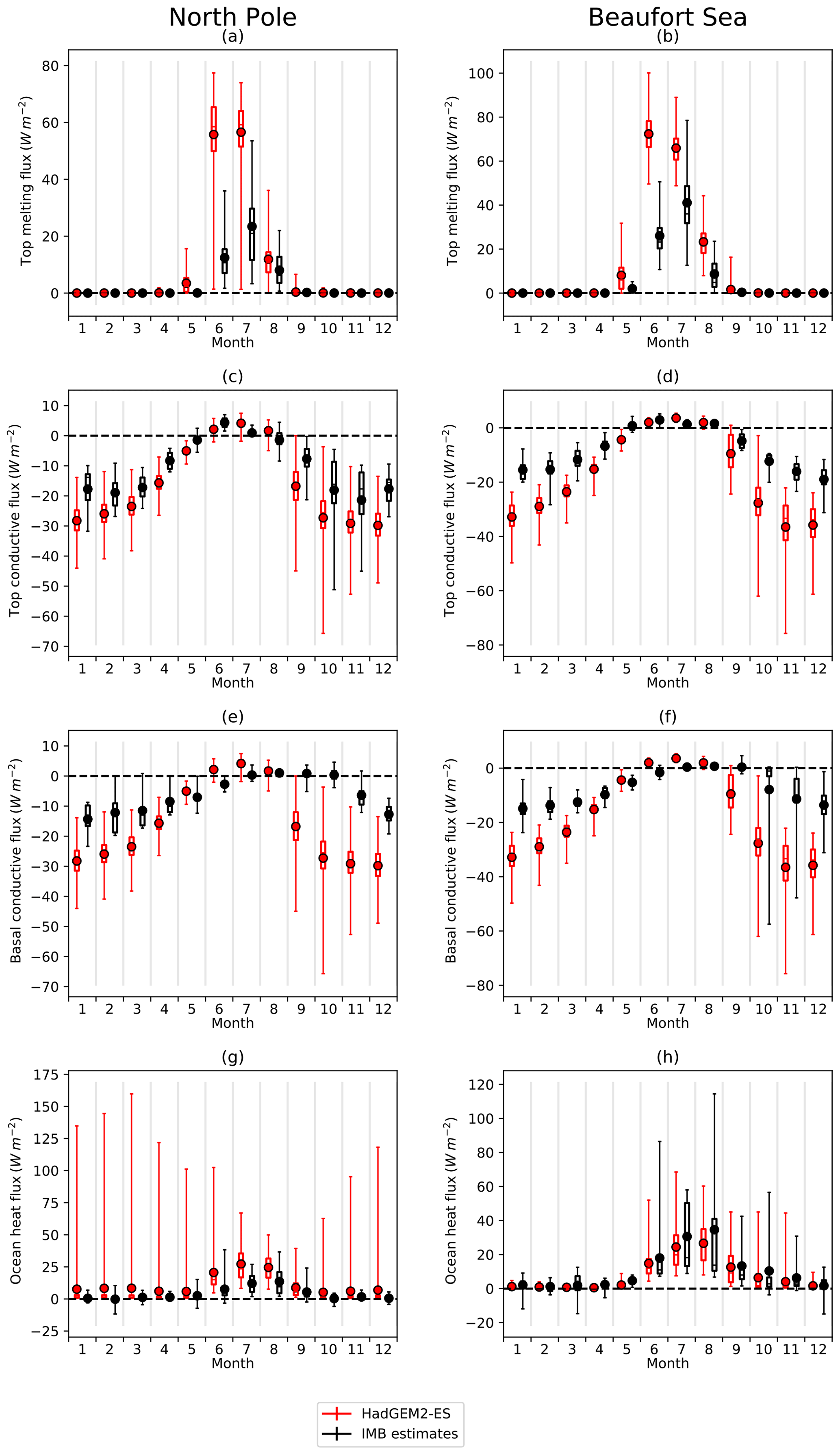
Figure 9Comparing distribution of (a, b) top melt, (c, d) top conductive flux, (e, f) basal conductive flux and (g, h) ocean heat flux from HadGEM2-ES (red) to those estimated from the IMB data (black), for the (a, c, e, g) North Pole and (b, d, f, h) Beaufort Sea regions.
The annual cycle of top conductive flux is broadly captured by HadGEM2-ES (Fig. 9c, d), with strongly negative values modelled in the autumn, winter and spring and weakly positive values in the summer. However, from September to May, modelled means are more strongly negative than observed means; for example, in the North Pole region in December a modelled mean of W m−2 is higher in magnitude than the IMB mean of W m−2. Ice thickness in HadGEM2-ES is known to be biased low in early winter (West et al., 2019), and in Sect. 4.2 below, the extent to which this bias is responsible for the conductive flux bias is investigated. The higher magnitude of conductive fluxes in winter in the Beaufort Sea region relative to the North Pole region is captured by the model; however, the higher values of fluxes in May and September in the Beaufort Sea region relative to the North Pole region are not captured. Modelled and observed flux distributions are significantly different in all months except February, March and November (North Pole region) and June, September and October (Beaufort Sea region).
Modelled values of basal conductive flux at each model grid box are identical to those of top conductive flux, due to the HadGEM2-ES zero-layer thermodynamics scheme. Consequently HadGEM2-ES overestimates the magnitude of basal conductive flux in autumn and winter more severely than it does top conductive flux (Fig. 9e, f). The overestimation is most severe during the autumn; in the Beaufort Sea region in October a mean modelled flux of W m−2 is much higher in magnitude than the mean observed flux of W m−2. As the basal conductive flux in the freezing season is the principal driver of ice growth, this suggests that HadGEM2-ES is likely to model substantially stronger ice growth during these months than was measured at the IMB sites. Modelled and observed fluxes are significantly different in all months and regions except, barely, in the North Pole region in August.
For the ocean heat flux, in the Beaufort Sea region the model produces a similar seasonal cycle to that estimated from the IMB data, with very small values in the winter and a wide range of positive values in the summer (Fig. 9g, h); only in April and May are the distributions significantly different. For the North Pole region however, two differences are apparent. Firstly, spread in winter ocean heat fluxes is much higher in the model, with a small number of very high fluxes; these occur near the southern boundary of the region, where the ice cover meets warmer water moving north through the Fram Strait. Secondly, modelled ocean heat fluxes in summer tend to be higher than those measured by the IMBs. For example, in July a modelled mean of 27.2±13.9 W m−2 compared to an observed mean of 12.1±7.4 W m−2. In the North Pole region, modelled and observed distributions are significantly different in all months except September.
The HadGEM2-ES ocean heat flux distributions are in fact similar between the North Pole and Beaufort Sea regions but evaluate differently because the IMB ocean heat fluxes in the North Pole region are much lower. In other words, the spatial variability in summer ocean heat fluxes suggested by the IMB data is not captured by the model. This may be related to late summer ice concentration biases in HadGEM2-ES: ice concentration is biased low in the North Pole region but not in the Beaufort Sea region. This would tend to cause a high bias in net SW absorption by the ocean mixed layer and, hence, a positive bias in ocean heat flux.
It is instructive also to examine how modelled oceanic heat convergence (OHC) compares to real-world estimates. Arctic Ocean heat convergence in HadGEM2-ES from 1980 to 1999 is 4.9 W m−2, roughly consistent with estimates of heat transport through the Fram Strait, the dominant pathway by which the Arctic Ocean gains heat (e.g. Schauer et al., 2004). However, oceanic heat convergence in the North Pole region (as defined in Fig. 3) is higher at 9.1 W m−2, while oceanic heat convergence in the Beaufort Sea region is lower at 1.6 W m−2. These patterns are consistent with most of the Arctic Ocean heat convergence being released relatively close to the Fram Strait and Barents Sea, the principal points of ingress of relatively warm Atlantic water. It is noteworthy that the large difference in OHC between the two regions is not mirrored in the ocean-to-ice heat flux. This is consistent with the finding by Keen et al. (2018) that much of the ocean-to-ice heat flux in HadGEM2-ES derives from direct solar heating, rather than OHC. Studies by Bitz et al. (2008), Perovich et al. (2008) and Steele et al. (2010) show this is likely to be true in the real world also. Hence differences in OHC are unlikely to contribute to differences in ocean–ice heat flux.
The model biases in summer top melt and winter conductive fluxes are larger than most of the uncertainties measured in Sect. 3.3. The model bias in top melt is of a similar magnitude to the uncertainty in top melting due to salinity, albeit in the opposite direction (higher salinities imply an even greater model bias). However, for the reasons stated in Sect. 3.3, the most meaningful comparison is obtained by considering the energy used in melting the whole of the top layer of ice, including the melting of brine pockets during sensible heating – equivalent to using a salinity of 0 in calculating top melting. Hence the model biases stated above – for the “standard configuration” – are likely to present the most accurate picture.
4.2 Links to sea ice and surface radiation simulation of HadGEM2-ES
A top melting bias of ∼40 W m−2 is estimated for the month of June in both the North Pole and Beaufort Sea regions. This is consistent with the finding of West et al. (2019) that June surface net shortwave (SW) radiation in the model was biased high relative to a variety of satellite and reanalysis datasets, by around 20 W m−2 over the Arctic Ocean on average. Relative to CERES-EBAF measurements from 2000 to 2013 (Loeb et al., 2009), HadGEM2-ES overestimates June net SW in the North Pole and Beaufort Sea regions by 30 and 9 W m−2 respectively. Owing to the recent trend to earlier onset of surface melt over the past 30 years (e.g. Markus et al., 2009) and attendant likely decrease in surface albedo, these biases are likely to be underestimated. Hence it is likely that a major part of the model bias in top melting can be explained by a model bias in net SW radiation. In West et al. (2019) it was shown that a tendency for surface melt onset to occur too early in HadGEM2-ES, reducing the surface albedo in a parameterization of the effect of melt ponds, was likely to be principally responsible for this.
The severe overestimation in magnitude of basal conductive fluxes during the early part of the melt season can be partly explained by the zero-layer thermodynamics scheme of HadGEM2-ES; the thermal inertia effect seen in the IMBs, whereby the basal conductive flux drops much more slowly in autumn than the top conductive flux, does not occur in the model. However, as the top conductive fluxes also tend to be considerably higher in the model than in the IMB estimates, the thermal inertia effect is likely to be only partially responsible. In West et al. (2019) two other model biases were identified as being likely to lead to a high bias in winter ice growth (analogous to the basal conductive flux bias): a negative bias in ice thickness during early winter and a negative bias in downwelling longwave (LW) radiation throughout the season. It was estimated that these biases were likely to lead to surface flux biases of order ∼10 W m−2 throughout the freezing season. Hence these are also likely to explain a portion of the basal conductive flux bias noted above.
The excessive modelled top melting and basal conductive fluxes identified would be likely to lead to ice growth and ice melting that are too strong, in winter and summer respectively, and an associated amplification of the ice thickness seasonal cycle. Such an amplification was identified in HadGEM2-ES by comparing modelled ice thickness to the forced ice–ocean model PIOMAS (Pan-Arctic Ice-Ocean Modeling and Assimilation System), as well as to estimates from satellites and submarines. Hence there is a high level of consistency between the model biases inferred from the IMB estimates and those inferred from the sea ice state and surface radiation evaluations in West et al. (2019). The IMB evaluation, however, provides additional insight to the picture, by providing consistent evaluation of previously unknown processes such as top melting. In addition, the IMB evaluation clearly identifies a role for the zero-layer thermodynamics scheme in driving a bias towards excess ice growth during the early winter in HadGEM2-ES.
4.3 The relationship between conductive flux, ice thickness and snow depth
Both top and basal conductive fluxes are strongly related to ice thickness, as thicker ice tends to have weaker temperature gradients than thinner ice under similar atmospheric conditions. Conductive fluxes are also related to snow depth for similar reasons. To examine the extent to which the HadGEM2-ES conductive flux biases are influenced by biases in ice thickness, conductive fluxes from November to March were aggregated into ice thickness bins, 20 cm wide and ranging from 0 to 4 m, in both IMBs and the model. HadGEM2-ES ice thicknesses are much lower than ice thicknesses sampled by the IMBs from November to March in both the North Pole and Beaufort Sea regions, with most of the “overlap” occurring in the range 1–2 m (Fig. 10).
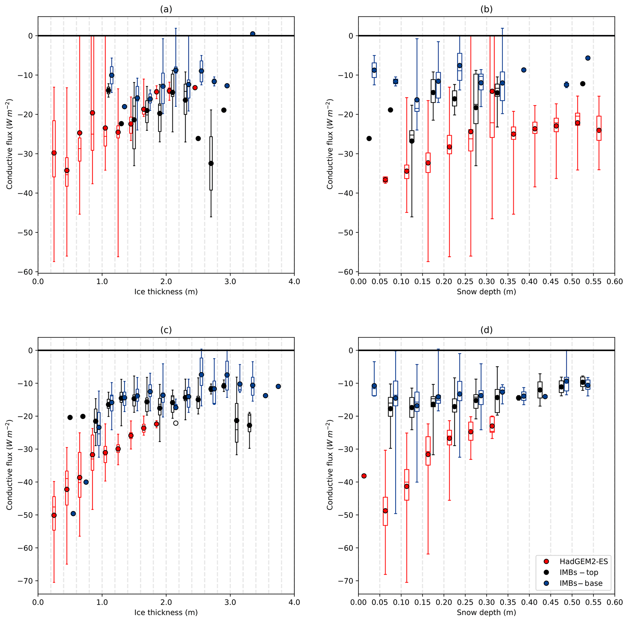
Figure 10Conductive fluxes plotted according to (a, c) ice thickness and (b, d) snow depth for the (a, b) North Pole and (c, d) Beaufort Sea regions.
For the North Pole region, IMB-measured top conductive flux is similar in magnitude to HadGEM2-ES conductive flux for the overlapping range of thicknesses, but IMB-measured basal conductive flux tends to be lower. For example, in the 1.4–16 m range, the IMB-measured top and basal conductive fluxes range from −33.0 to −11.9 and −24.0 to −10.8 W m−2 respectively, while the HadGEM2-ES conductive flux ranges from −15.6 to −26.6 W m−2. As above, this suggests that the uniform conductive flux assumption of HadGEM2-ES is important in driving excessive ice growth in this model. However, in the Beaufort Sea region both top and basal conductive fluxes from the IMBs are much lower than HadGEM2-ES even in the region of overlapping thicknesses. For example, in the 1.4–1.6 m range, the IMB-measured top and basal conductive fluxes range from −18.8 to −7.8 and −18.4 to −8.3 W m−2 respectively, while the HadGEM2-ES conductive flux ranges from −30.0 to −21.4 W m−2. This indicates that in the Beaufort Sea at least, ice thickness biases and the uniform conductive flux assumption are not the only factors driving excessive ice growth; biases in atmospheric thermal forcing are also at work.
The HadGEM2-ES conductive fluxes display an inverse relationship with ice thickness. Cells with thinner ice tend to have higher conductive flux (Fig. 10a, b); in the Beaufort Sea region for example, the correlation coefficient between conductive flux and the logarithm of ice thickness is 0.66. Curiously, there is no sign of a similar relationship in the IMBs in either region; in the Beaufort Sea region the correlation coefficient between the log of ice thickness and top (basal) conductive flux is small and not significant at 0.25 (−0.16). In particular, both regions exhibit large numbers of IMB measurements with high ice thicknesses and high top conductive fluxes. In most cases these points are associated with strong ice cooling and a very low basal conductive flux.
When conductive flux is compared to snow depth, it can be seen that similar snow depths are associated with much greater conductive fluxes in HadGEM2-ES than in the IMB data (Fig. 10c, d), indicating that snow depth biases are unlikely to be a major contributor to the conductive flux biases. A similar inverse relationship between conductive flux and snow depth is seen in HadGEM2-ES, stronger in the Beaufort Sea than at the North Pole. Unlike with the ice thickness, there is the suggestion of a similar relationship in the IMB data, with the 10–15 cm (5–10 cm) category in the North Pole (Beaufort Sea) displaying much higher conductive fluxes than are present in the other categories. No data points with high snow depths display high conductive fluxes. As a result, the correlation between top (basal) conductive flux and the log of ice thickness in the IMB estimates is 0.47 (0.48).
The comparison of HadGEM2-ES modelled fluxes to those inferred from the IMB measurements reveals several potential model biases, notably the overestimation of top melt flux in June and July and the overestimation of the magnitude of basal conductive flux in the early freezing season. In this section the accuracy of this method of model bias estimation is discussed.
The model flux distributions evaluated represent area-weighted means over the ice-covered fractions of grid cells, each of order 10–100 km in width, chosen to cover the North Pole and Beaufort Sea regions as defined in Sect. 2. The “true model bias” would represent the difference between this and the average flux over ice-covered regions for each month in the 1980–1999 period. By contrast, the IMB-measured means are derived from a relatively small number of single-point measurements from these regions (points that tend to move position during an individual month, with the general ice flow), most from a period somewhat later than 1980–1999. To assess the accuracy of the model biases inferred, a method of estimating the order of magnitude of the likely error in the IMB estimated mean fluxes is required.
One source of error derives from the temporal offset in the IMB measurements relative to the model. To assess the impact of this, we compare the HadGEM2-ES vertical ice fluxes from the period 1980–1999 to those from the period 2000–2015, during which most of the IMB measurements were taken (as the historical experiments end in 2005; the RCP8.5 experiment was used from 2006 onwards). Flux anomalies in the later period relative to the earlier period are mostly small (below 2 W m−2 in magnitude) in both regions. However, there is a significant negative anomaly in July top melting, −6 and −9 W m−2 in the North Pole and Beaufort Sea regions respectively. There is also a positive anomaly in September basal conductive flux (3 W m−2 in both regions), and in the Beaufort Sea moderate basal conductive flux anomalies continue into the winter, being 5, 3, −4 and −2 W m−2 from October to January respectively. These anomalies are likely to reflect earlier melting and later freezing of ice in this region. They are small in size compared to the HadGEM2-ES model biases but suggest that the temporal bias may cause model top melting bias in July – and Beaufort Sea basal conductive flux in autumn – to be slightly overstated.
A potentially more serious source of error is sampling – bias would be introduced if the IMB measurements were systematically over- or undersampling locations with higher than average flux in a particular month. The Arctic sea ice cover is highly heterogeneous, with ice conditions varying substantially over all scales. For most variables (for example snow thickness, ice salinity or ice albedo), it is difficult to assess whether the variability in the ice pack is sufficiently sampled by the IMB measurements, due either to a lack of reference datasets or to an inability to estimate these variables at the IMB locations. However, the degree to which the ice thickness distribution (which affects conductive fluxes in particular) is correctly sampled by the IMBs can be assessed. The effect of errors in the ice thickness distribution on the IMB-measured fluxes is estimated in Appendix A and is shown to be small compared to the model biases identified. We note that the ice thickness distribution sampling bias is likely to be particularly strong (relative to other variables) due to the deliberate placing of IMBs in level multiyear ice and due to the Lagrangian movement of the IMBs combined with the generally short lifetime of thin ice floes, which tend to grow quickly in winter and melt quickly in summer. It is proposed that given the effect of this bias is weak, it is likely that the effect of other, not deliberately introduced, biases is weaker still and that the model biases identified in Sect. 4 are likely to be robust features.
Around 500 estimates of monthly mean top melt, top conduction, basal conduction and ocean heat flux have been estimated from data measured by the Arctic IMB network, with the number of estimates available for each month ranging from 25 to 59. The distributions capture seasonal and spatial variability in the vertical fluxes analysed but do not contain sufficient data points to capture interannual variability. Comparison of modelled fluxes to observed fluxes in the two densely sampled regions in the North Pole and Beaufort Sea reveals substantial model biases, notably to high top melt fluxes in summer and to high (negative) basal conductive fluxes in autumn and early winter. Uncertainty in the IMB fluxes due to parameters of the analysis and biases due to inadequate sampling of thin and very thick ice types are likely to be small relative to the model biases identified.
The flux biases are consistent with an evaluation of the sea ice simulation of HadGEM2-ES that identified an over-amplified seasonal cycle in ice thickness, with model ice growth and melt biased high in winter and summer respectively, as well as a high model bias in net SW radiation in June, a low bias in net LW radiation throughout the winter, and a low model bias in ice thickness in autumn and early winter. The IMB analysis confirms that the net SW bias is likely to cause overly strong ice thinning during summer via anomalously strong top melting of ice. The IMB analysis also allows the effect of biases in ice thickness, snow depth and atmospheric conditions, as well as the effect of the uniform conductive flux assumption, on the conductive fluxes to be separately examined. In this way it is confirmed that both low ice thickness and cold atmospheric conditions are likely to be driving anomalously strong winter ice growth via the basal conductive flux, both conclusions already suggested by West et al. (2019). However, the IMB analysis also suggests that the zero-layer thermodynamic scheme of HadGEM2-ES plays a role in promoting this anomalously strong ice growth. The IMB analysis also provides evidence that snow depth biases are not important in driving the ice growth biases of HadGEM2-ES.
The calculated IMB fluxes hence offer a valuable tool for increasing understanding of sea ice simulations in coupled models, as they allow detailed examination of the links between atmospheric forcing of sea ice and the resulting sea ice state. This is particularly the case for the upcoming Phase 6 of the Coupled Model Intercomparison Project (CMIP6), for which diagnostics of ice energy and mass fluxes, such as top melting and conduction, have been requested for all sea ice models participating in this experiment (Notz et al., 2016). Understanding of the processes leading to biases in a given sea ice state enables better understanding of modelled sea ice spread in the present day and in the future and may, therefore, also allow better understanding of future projections in sea ice state.
The greatest source of uncertainty in estimating the IMB fluxes derives from lack of knowledge of ice salinity at the measurement sites and, therefore, the thermodynamic properties of conductivity and heat capacity. A method of measuring salinity at the IMB sites would greatly reduce the uncertainty in the IMB estimates, particularly for ocean heat flux, enhancing the usefulness of this dataset as a tool for model evaluation.
An analysis of the distribution of monthly mean ice thicknesses sampled by the IMBs finds that most lie in the range 1.4–3.6 m. However, analysis of submarine measurements of ice thickness in the central and western Arctic from 1981 to 2000, as collated by Rothrock et al. (2008), shows a substantial proportion of ice to be of thickness outside these bounds. In order to estimate the effect of this sampling bias, we use the following simple model. The thickness distribution is discretized, in a similar manner to HadGEM2-ES, by separating ice into five thickness categories, with minimum thickness bounds at 0, 0.6, 1.4, 2.4 and 3.6 m. Given a mean flux for month m and region r that is estimated from the IMBs by averaging all fluxes for that month and region, the total observational error can be characterized as
where is the actual value of that flux, averaged over the region and month in question, for the period 1993–2015. The mean flux can be further split into thickness categories by setting
where the are the average IMB flux over month m, region r, and category i, is the total number of IMB fluxes in month m, region r, and category i, and is the total number of IMB fluxes in month m and region r.
Similarly, the actual flux values can be written as
where is the average fraction of ice in month m and region r that is in category i (expressed as a proportion of average fraction of ice in the region).
It can be seen that acts as an IMB-based estimate of and that the error in due to the ice thickness sampling bias is exactly that due to the error in this estimate. Hence we can characterize the sampling error by expressing Ferr in terms of systematic and sampling errors in the following way:
where Ferr_sample captures the flux error due to ice thickness sampling; Ferr_systematic describes the error due to inaccuracy in the IMBs estimating F for each particular category, effectively capturing the remaining observational error that is beyond the scope of the current analysis.
To estimate Ferr_sample, we first need estimates of , the real-world proportion of ice in a given thickness category for each region and month, for which we use submarine measurements (National Snow and Ice Data Center, 2019), which capture small-scale variation in sea ice thickness. Ice thickness measurements in each category are collected for each month and region and are used to generate an estimate of . In practice, measurements are abundant during spring and autumn but sparse during summer and nonexistent during winter. To alleviate this problem, we interpolate using a 5-month binomial mean, weighted by number of measurements, in order to produce a smooth seasonal cycle, motivated by the observation that maximum and minimum ice thickness values often occur during spring and autumn respectively. The resulting seasonal cycles of are shown in Fig. S2.
Secondly, estimates of , representative average fluxes for each thickness category, are required. To calculate representative fluxes of conduction, we combine a simple model of the relationship between conductive fluxes and ice and snow thickness with the IMB measurements of conduction. The surface flux is approximated by linearizing the dependence on surface temperature Tsfc, referenced to 0 ∘C. The surface flux is set equal to the top conductive flux Fcondtop, and a constant rate of change of conductive flux from the top to the basal surface of the ice is assumed, such that , where Fcondbot represents basal conductive flux, Tbot is the ice base temperature, and is the thermal insulance of the ice–snow column – with hice and hsnow being ice and snow thickness and kice and ksnow ice and snow conductivity respectively. Eliminating Tsfc from the above equations gives
where and .
Equation (A5) can be combined with the IMB estimates of conductive fluxes and the snow and ice thickness to produce, for each monthly mean IMB measurement, an associated value of Fatmos, a measure of the atmospheric forcing on the ice that is independent of small-scale variations in ice thickness. Hence for each month and region, a distribution in Fatmos can be produced; mean values of this can be fed back into the simple model to produce an average conductive flux that would be expected for each ice thickness category. The average conductive flux is then multiplied by , as estimated above, and summed over categories to produce the flux error .
The resulting flux bias is below 1 W m−2 in magnitude year round in the North Pole region. It is slightly larger in the Beaufort Sea in winter time, achieving values of −1.5 to −1 W m−2 from November to February. The values are small compared to the model–observation differences identified in Sect. 4, and so we conclude that the ice thickness sampling bias does not seriously affect ability to evaluate modelled conductive fluxes.
A less strong – but still discernible – relationship exists between top melt flux and ice thickness, due to ice albedo tending to be lower for thinner ice. However, this effect is likely to be associated with a significant difference in albedo only for the thinnest category of ice – and then only in the absence of snow (e.g. Ebert et al., 1995). To estimate this effect, we use an average albedo of 0.55 for bare ice in the top four thickness categories and 0.35 in the lowest category, based on observed values reviewed and collated by Pirazzini (2008). We assume that ice is snow-covered 80 % of the time from October to May (with a corresponding albedo of 0.85), 50 % of the time in June and September, and 20 % of the time in July and August. Finally, we calculate mean values of downwelling SW radiation for the North Pole and Beaufort Sea regions from CERES-EBAF from 2000 to 2013 and multiply these by the albedo differences implied by the anomaly of ice fraction in category 1. With this method, a maximum flux bias of −3 W m−2 is estimated for the North Pole region, in July, and −2 W m−2 for the Beaufort Sea region, also in July. Again, this anomaly is small compared to the model–observation differences seen in Sect. 4, and it is concluded that the sampling bias similarly does not affect ability to evaluate modelled top melting.
An estimate of the influence of the sampling bias on ocean heat flux estimates is more difficult, due to a less clear relationship between ice thickness and the ocean heat flux and to the frequent presence of rapid changes in ice thickness during the months in which ocean heat flux is highest (July and August). It is likely that very small ice thicknesses are associated with elevated ocean heat flux in the summer months due to greater solar penetration through ice. However, the ice thickness sampling bias is at its least severe during the summer months, as thinner ice is sampled by the IMBs simply through the melting of originally thicker floes on which the IMBs were placed. In addition, thinning ice, which induces a particularly high ocean heat flux, is likely to melt out quickly and contribute a correspondingly small fraction to the ice thickness distribution.
We examined the sensitivity of the average ocean heat fluxes to this issue by assuming ocean heat fluxes in category 1 to be systematically larger than those in the remaining categories (as diagnosed from the IMBs) by a factor λ. With λ=3, August ocean heat fluxes in the Beaufort Sea region are on average 80 W m−2 greater in category 1 than in thicker ice categories; it is unlikely that the solar penetration effect could be associated with larger flux differences than this. The largest average flux bias associated with this effect is then −6.3 W m−2, also seen in August in the Beaufort Sea region. Hence this could be taken as a reasonable upper bound for the effect of the sampling bias on ocean heat fluxes. It is smaller in magnitude than the model ocean heat flux biases diagnosed, although the difference is less than those for the top melt and conductive fluxes.
The code used to analyse the IMB data is published in two repositories, corresponding to two stages of the analysis. The code used to read, quality control and process the data into consistent quantities on consistent time points can be downloaded from https://doi.org/10.5281/zenodo.3975692 (West, 2020a). The code used to produce datasets of monthly mean energy fluxes from this processed data can be downloaded from https://doi.org/10.5281/zenodo.3971736 (West, 2020b). In addition, the code with which Figs. 3–10, S1 and S2, were produced is published at https://doi.org/10.5281/zenodo.3947782 (West, 2020c).
The raw IMB data are publicly available and can be downloaded from http://imb-crrel-dartmouth.org/results/ (last access: 20 April 2020, Perovich et al., 2020). The processed IMB data and the derived dataset of monthly mean fluxes are published with this revision at https://doi.org/10.5281/zenodo.3773811 (West, 2020d) and https://doi.org/10.5281/zenodo.3773997 (West, 2020e) respectively. The diagnostics from HadGEM2-ES used in this study are not publicly available. However, they can be made available upon request to the author.
The supplement related to this article is available online at: https://doi.org/10.5194/gmd-13-4845-2020-supplement.
The IMB-derived fluxes were calculated and the subsequent model evaluation performed by AW, with code reviewed by EB before publication. The analysis of sampling error in the Appendix was designed and carried out by AW. The paper was written in its final form by AW with assistance from MC and EB.
The author declares that there is no conflict of interest.
The authors thank the two anonymous reviewers for their thorough reading of the first revision of this study and for their helpful and constructive feedback.
This work was supported by the Joint UK BEIS–Defra Met Office Hadley Centre Climate Programme (GA01 101) and the European Commission, H2020 Research & Innovation programme (APPLICATE (grant no. 727862)). Mat Collins was supported by National Environmental Research Council (NERC) award “Robust Spatial Projections of Real-World Climate Change” (award no. NE/N018486/1).
This paper was edited by James R. Maddison and reviewed by two anonymous referees.
Alexandrov, V., Sandven, S., Wahlin, J., and Johannessen, O. M.: The relation between sea ice thickness and freeboard in the Arctic, The Cryosphere, 4, 373–380, https://doi.org/10.5194/tc-4-373-2010, 2010.
Bitz, C. M.: Some Aspects of Uncertainty in Predicting Sea Ice Thinning, in: Arctic Sea Ice Decline: Observations, Projections, Mechanisms, and Implications, edited by: DeWeaver, E. T., Bitz, C. M., and Tremblay, L.-B., American Geophysical Union, Washington, D.C., https://doi.org/10.1029/180GM06, 2008.
Bitz, C. M. and Lipscomb, W. H.: An energy-conserving thermodynamic model of sea ice, J. Geophys. Res., 104, 15669–15677, https://doi.org/10.1029/1999JC900100, 1999.
Bliss, A. C., Steele, M., Peng, G., Meier, W. N., and Dickinson, S.: Regional variability of Arctic sea ice seasonal change climate indicators from a passive microwave climate data record, Environ. Res. Lett., 14, 045003, https://doi.org/10.1088/1748-9326/aafb84, 2019.
Collins, W. J., Bellouin, N., Doutriaux-Boucher, M., Gedney, N., Halloran, P., Hinton, T., Hughes, J., Jones, C. D., Joshi, M., Liddicoat, S., Martin, G., O'Connor, F., Rae, J., Senior, C., Sitch, S., Totterdell, I., Wiltshire, A., and Woodward, S.: Development and evaluation of an Earth-System model – HadGEM2, Geosci. Model Dev., 4, 1051–1075, https://doi.org/10.5194/gmd-4-1051-2011, 2011.
Cox, G. F. N. and Weeks, W. F.: Equations for Determining the Gas and Brine Volume in Sea Ice Samples, J. Glaciol., 29, 306–316, https://doi.org/10.3189/S0022143000008364, 1983.
Ebert, E. E., Schramm, J. L., and Curry, J. C.: Disposition of solar radiation in sea ice and the upper ocean, J. Geophys. Res., 100, 15965–15975, https://doi.org/10.1029/95JC01672, 1995.
Hunke, E. C. and Dukowicz, J. K.: An Elastic–Viscous–Plastic Model for Sea Ice Dynamics, J. Phys. Oceanogr., 27, 1849–1867, https://doi.org/10.1175/1520-0485(1997)027<1849:AEVPMF>2.0.CO;2, 1997.
Keen, A. and Blockley, E.: Investigating future changes in the volume budget of the Arctic sea ice in a coupled climate model, The Cryosphere, 12, 2855–2868, https://doi.org/10.5194/tc-12-2855-2018, 2018.
Kwok, R.: Arctic sea ice thickness, volume, and multiyear ice coverage: losses and coupled variability (1958–2018), Environ. Res. Lett., 13, 105005, https://doi.org/10.1088/1748-9326/aae3ec, 2018.
Lei, R., Li, N., Heil, P., Cheng, B., Zhang, Z., and Sun, B.: Multiyear sea ice thermal regimes and oceanic heat flux derived from an ice mass balance buoy in the Arctic Ocean, J. Geophys. Res.-Oceans, 119, 537–547, https://doi.org/10.1002/2012JC008731, 2014.
Lei, R., Cheng, B., Heil, P., Vihma, T., Wang, J., Ji, Q., and Zhang, Z.: Seasonal and Interannual Variations of Sea Ice Mass Balance From the Central Arctic to the Greenland Sea, J. Geophys. Res.-Oceans, 123, 2422–2439, https://doi.org/10.1002/2017JC013548, 2018.
Lindsay, R. and Schweiger, A.: Arctic sea ice thickness loss determined using subsurface, aircraft, and satellite observations, The Cryosphere, 9, 269–283, https://doi.org/10.5194/tc-9-269-2015, 2015.
Loeb, N. G., Wielicki, B. A., Doelling, D. R., Louis Smith, G., Keyes, D. F., Kato, S., Manalo-Smith, N., and Wong, T.: Toward Optimal Closure of the Earth's Top-of-Atmosphere Radiation Budget, J. Climate, 22, 748–766, https://doi.org/10.1175/2008JCLI2637.1, 2009.
Markus, T., Stroeve, J. C., and Miller, J.: Recent changes in Arctic sea ice melt onset, freezeup, and melt season length, J. Geophys. Res., 114, C12024, https://doi.org/10.1029/2009JC005436, 2009.
Maykut, G. A. and Untersteiner, N.: Some results from a time-dependent thermodynamic model of sea ice, J. Geophys. Res., 76, 1550–1575, https://doi.org/10.1029/JC076i006p01550, 1971.
McLaren, A. J., Banks, H. T., Durman, C. F., Gregory, J. M., Johns, T. C., Keen, A. B., Ridley, J. K., Roberts, M. J., Lipscomb, W. H., Connolley, W. M., and Laxon, S. W.: Evaluation of the sea ice simulation in a new coupled atmosphere-ocean climate model (HadGEM1), J. Geophys. Res., 111, C12014, https://doi.org/10.1029/2005JC003033, 2006.
National Snow and Ice Data Center (comp.): Submarine Upward Looking Sonar Ice Draft Profile Data and Statistics, Version 1, NSIDC: National Snow and Ice Data Center, Boulder, Colorado, USA, https://doi.org/10.7265/N54Q7RWK, 2019.
Notz, D.: How well must climate models agree with observations?, Philos. T. Roy. Soc. A, 373, 20140164, https://doi.org/10.1098/rsta.2014.0164,
Notz, D., McPhee, M. G., Worster, M. G., Maykut, G. A., Schlunzen, K. H., and Eicken, H.: Impact of underwater-ice evolution on Arctic summer sea ice, J. Geophys. Res., 108, 3223, https://doi.org/10.1029/2001JC001173, 2003.
Notz, D., Jahn, A., Holland, M., Hunke, E., Massonnet, F., Stroeve, J., Tremblay, B., and Vancoppenolle, M.: The CMIP6 Sea-Ice Model Intercomparison Project (SIMIP): understanding sea ice through climate-model simulations, Geosci. Model Dev., 9, 3427–3446, https://doi.org/10.5194/gmd-9-3427-2016, 2016.
Olonscheck, D. and Notz, D.: Consistently Estimate Internal Climate Variability from Climate Model Simulations, J. Climate, 30, 9555–9573, https://doi.org/10.1175/JCLI-D-16-0428.1, 2018.
Ono, N.: Specific heat and heat of fusion of sea ice, in: Physics of Snow and Ice, edited by: Oura, H., Institute of Low Temperature Science, Hokkaido, Japan, 1, 599–610, 1967.
Perovich, D. and Elder, B.: Estimates of ocean heat flux at SHEBA, Geophys. Res. Lett., 29, 58-1–58-4, https://doi.org/10.1029/2001GL014171, 2002.
Perovich, D. and Richter-Menge, J. A.: From points to Poles: extrapolating point measurements of sea-ice mass balance, Ann. Glaciol., 44, 188–192, https://doi.org/10.3189/172756406781811204, 2006.
Perovich, D., Richter-Menge, J. A., Jones, K. F., and Light, B.: Sunlight, water, and ice: Extreme Arctic sea ice melt during the summer of 2007, Geophys. Res. Lett., 35, L11501, https://doi.org/10.1029/2008GL034007, 2008.
Perovich, D., Richter-Menge, J., and Polashenski, C.: Observing and understanding climate change: Monitoring the mass balance, motion, and thickness of Arctic sea ice, The CRREL-Dartmouth Mass Balance Buoy Program (Cold Regions Research and Engineering Laboratory, Thayer School of Engineering at Dartmouth), available at: http://imb-crrel-dartmouth.org/results/, last access: 20 April 2020.
Pirazzini, R.: Factors controlling the surface energy budget over snow and ice, Finnish Meteorological Institute, Contributions No. 75, p. 22, 2008.
Planck, C. J., Whitlock, J., Polashenski, C., and Perovich, D.: The evolution of the seasonal Ice Mass Balance Buoy, Cold Reg. Sci. Technol., 165, 102792, https://doi.org/10.1016/j.coldregions.2019.102792, 2019.
Pringle, D. J., Eicken, H., Trodahl, H. J., and Backstrom, L. G. E.: Thermal conductivity of landfast Antarctic and Arctic sea ice, J. Geophys. Res., 112, C04017, https://doi.org/10.1029/2006JC003641, 2007.
Provost, C., Sennéchael, N., Miguet, J., Itkin, P., Rösel, A., Koenig, Z., Villacieros‐Robineau, N., and Granskog, M. A.: Observations of flooding and snow‐ice formation in a thinner Arctic sea‐ice regime during the N‐ICE2015 campaign: Influence of basal ice melt and storms, J. Geophys. Res.-Oceans, 122, 7115–7134, https://doi.org/10.1002/2016JC012011, 2017.
Rösel, A., Itkin, P., King, J., Divine, D., Wang, C., Granskog, M. A., Krumpen, T., and Gerland, S.: Thin Sea Ice, Thick Snow, and Widespread Negative Freeboard Observed during NICE-2015 north of Svalbard, J. Geophys. Res.-Oceans, 123, 1156–1176, https://doi.org/10.1002/2017JC012865, 2018.
Rothrock, D. A., Percival, D. B., and Wensnahan, M.: The decline in arctic sea ice thickness: Separating the spatial, annual, and interannual variability in a quarter century of submarine data, J. Geophys. Res., 113, C05003, https://doi.org/10.1029/2007JC004252, 2008.
Schauer, U., Fahrbach, E., Osterhus, S., and Rohardt, G.: Arctic warming through Fram Strait: Oceanic heat transport from 3 years of measurements, J. Geophys. Res., 109, C06026, https://doi.org/10.1029/2003JC001823, 2004.
Schwarzacher, W.: Pack ice studies in the Arctic Ocean, J. Geophys. Res., 64, 2357–2367, https://doi.org/10.1029/JZ064i012p02357, 1959.
Semtner Jr., A. J.: A Model for the Thermodynamic Growth of Sea Ice in Numerical Investigations of Climate, J. Phys. Oceanogr., 6, 379–389 https://doi.org/10.1175/1520-0485(1976)006<0379:AMFTTG>2.0.CO;2, 1976.
Shu, Q., Song, Z., and Qiao, F.: Assessment of sea ice simulations in the CMIP5 models, The Cryosphere, 9, 399–409, https://doi.org/10.5194/tc-9-399-2015, 2015.
Steele, M., Zhang, J., and Ermold, W.: Mechanisms of summer Arctic Ocean warming, J. Geophys. Res., 115, C11004, https://doi.org/10.1029/2009JC005849, 2010.
Stroeve, J., Barrett, A., Serreze, M., and Schweiger, A.: Using records from submarine, aircraft and satellites to evaluate climate model simulations of Arctic sea ice thickness, The Cryosphere, 8, 1839–1854, https://doi.org/10.5194/tc-8-1839-2014, 2014.
Stroeve, J. C., Kattsov, V., Barrett, A., Serreze, M., Pavlova, T., Holland, M. M., and Meier, W. N.: Trends in Arctic sea ice extent from CMIP5, CMIP3 and observations. Geophys. Res. Lett., 39, L16502, https://doi.org/10.1029/2012GL052676, 2012.
Swart, N. C., Fyfe, J. C., Hawkins, E., Kay, J. E., and Jahn, A.: Influence of internal variability on Arctic sea ice trends, Nat. Clim. Change, 5, 86–89, https://doi.org/10.1038/nclimate2483, 2015.
The HadGEM2 Development Team: G. M. Martin, Bellouin, N., Collins, W. J., Culverwell, I. D., Halloran, P. R., Hardiman, S. C., Hinton, T. J., Jones, C. D., McDonald, R. E., McLaren, A. J., O'Connor, F. M., Roberts, M. J., Rodriguez, J. M., Woodward, S., Best, M. J., Brooks, M. E., Brown, A. R., Butchart, N., Dearden, C., Derbyshire, S. H., Dharssi, I., Doutriaux-Boucher, M., Edwards, J. M., Falloon, P. D., Gedney, N., Gray, L. J., Hewitt, H. T., Hobson, M., Huddleston, M. R., Hughes, J., Ineson, S., Ingram, W. J., James, P. M., Johns, T. C., Johnson, C. E., Jones, A., Jones, C. P., Joshi, M. M., Keen, A. B., Liddicoat, S., Lock, A. P., Maidens, A. V., Manners, J. C., Milton, S. F., Rae, J. G. L., Ridley, J. K., Sellar, A., Senior, C. A., Totterdell, I. J., Verhoef, A., Vidale, P. L., and Wiltshire, A.: The HadGEM2 family of Met Office Unified Model climate configurations, Geosci. Model Dev., 4, 723–757, https://doi.org/10.5194/gmd-4-723-2011, 2011.
Thorndike, A. S., Rothrock, D. A., Maykut, G. A., and Colony, R.: The thickness distribution of sea ice, J. Geophys. Res., 80, 4501–4513, https://doi.org/10.1029/JC080i033p04501, 1975.
Wang, M. and Overland, J. E.: A sea ice free summer Arctic within 30 years: An update from CMIP5 models, Geophys. Res. Lett., 39, L18501, https://doi.org/10.1029/2012GL052868, 2012.
West, A. E.: IMBS_MO, Zenodo, https://doi.org/10.5281/zenodo.3975692, 2020a.
West, A. E.: IMBS_Stage2_modeleval_MO, Zenodo, https://doi.org/10.5281/zenodo.3971736, 2020b.
West, A. E.: Figure code for publication 'Using Arctic ice mass balance buoys for evaluation of modelled ice energy fluxes', Zenodo, https://doi.org/10.5281/zenodo.3947782, 2020c.
West, A. E.: Arctic ice mass balance buoy data for use in calculating quantities to evaluate climate models, Version v1_april_2020, Zenodo, https://doi.org/10.5281/zenodo.3773811, 2020d.
West, A. E.: Monthly mean variables derived from Arctic Ice Mass Balance Buoy data, for evaluation of sea ice models, Version v1_april_2020, Zenodo, https://doi.org/10.5281/zenodo.3773997, 2020e.
West, A., Collins, M., Blockley, E., Ridley, J., and Bodas-Salcedo, A.: Induced surface fluxes: a new framework for attributing Arctic sea ice volume balance biases to specific model errors, The Cryosphere, 13, 2001–2022, https://doi.org/10.5194/tc-13-2001-2019, 2019.
Wettlaufer, J. S.: Heat flux at the ice-ocean interface, J. Geophys. Res., 96, 7215–7236, https://doi.org/10.1029/90JC00081, 1991.
- Abstract
- Introduction
- Calculating monthly mean energy fluxes from the IMBs
- Description of monthly mean flux distributions from the IMBs
- Evaluating modelled sea ice using the IMB-derived fluxes
- Representativeness of the IMB-estimated fluxes
- Conclusions
- Appendix A: The ice thickness sampling bias and its effect on flux distributions
- Code availability
- Data availability
- Author contributions
- Competing interests
- Acknowledgements
- Financial support
- Review statement
- References
- Supplement