the Creative Commons Attribution 4.0 License.
the Creative Commons Attribution 4.0 License.
 | 05 Oct 2020
Impact of the ice thickness distribution discretization on the sea ice concentration variability in the NEMO3.6–LIM3 global ocean–sea ice model
Eduardo Moreno-Chamarro
Pablo Ortega
François Massonnet
This study assesses the impact of different sea ice thickness distribution (ITD) discretizations on the sea ice concentration (SIC) variability in ocean stand-alone NEMO3.6–LIM3 simulations. Three ITD discretizations with different numbers of sea ice thickness categories and boundaries are evaluated against three different satellite products (hereafter referred to as “data”). Typical model and data interannual SIC variability is characterized by K-means clustering both in the Arctic and Antarctica between 1979 and 2014. We focus on two seasons, winter (January–March) and summer (August–October), in which correlation coefficients across clusters in individual months are largest. In the Arctic, clusters are computed before and after detrending the series with a second-degree polynomial to separate interannual from longer-term variability. The analysis shows that, before detrending, winter clusters reflect the SIC response to large-scale atmospheric variability at both poles, while summer clusters capture the negative and positive trends in Arctic and Antarctic SIC, respectively. After detrending, Arctic clusters reflect the SIC response to interannual atmospheric variability predominantly. The cluster analysis is complemented with a model–data comparison of the sea ice extent and SIC anomaly patterns.
The single-category discretization shows the worst model–data agreement in the Arctic summer before detrending, related to a misrepresentation of the long-term melting trend. Similarly, increasing the number of thin categories reduces model–data agreement in the Arctic, due to a poor representation of the summer melting trend and an overly large winter sea ice volume associated with a net increase in basal ice growth. In contrast, more thin categories improve model realism in Antarctica, and more thick ones improve it in central Arctic regions with very thick ice. In all the analyses we nonetheless identify no optimal discretization. Our results thus suggest that no clear benefit in the representation of SIC variability is obtained from increasing the number of sea ice thickness categories beyond the current standard with five categories in NEMO3.6–LIM3.
- Article
(17514 KB) - Full-text XML
-
Supplement
(3852 KB) - BibTeX
- EndNote


Analysis of recent observations has allowed identification of different drivers of sea ice variability. Interannual sea ice variability, for example, has been associated primarily with changes in atmospheric and oceanic circulation: atmospheric variability related to large-scale atmospheric modes, such as the North Atlantic Oscillation (NAO) or Siberian High in the Northern Hemisphere and the Southern Annular Mode over Antarctica, can drive changes in the sea ice both dynamically and thermodynamically (e.g., Rigor et al., 2002; Rigor and Wallace, 2004; Ogi et al., 2007; Yuan and Li, 2008; Wang et al., 2009; Hobbs and Raphael, 2010; Holland and Kwok, 2012; Renwick et al., 2012; Kohyama and Hartmann, 2016; Lynch et al., 2016; Close et al., 2017; Blackport et al., 2019; Olonscheck et al., 2019). Similarly, interannual changes in ocean heat transport to high latitude can contribute to anomalous episodes of Arctic sea ice melting in both the Atlantic and Pacific sectors (e.g., Hibler, 1986; Venegas and Mysak, 2000; Ingvaldsen et al., 2004a; b; Woodgate et al., 2010; Schlichtholz, 2011). On longer timescales, the accelerating thinning in Arctic sea ice (Comiso et al., 2008; Serreze and Stroeve, 2015) might be modulated by lower-frequency variability in modes such as the NAO (e.g., Delworth et al., 2016) or Atlantic multidecadal variability (e.g., Day et al., 2012; Drinkwater et al., 2014; Miles et al., 2014). Accurately capturing the complex range of variability in sea ice, together with the potential impacts on the lower-latitude climate (e.g., Screen, 2013), demands a realistic representation of sea ice in climate models.
One among the many crucial features of sea ice to ensure its realistic representation is its thickness heterogeneity, which determines other important physical properties, such as ice's salt and heat content, resistance to deformation and fracture, and melting and growth rates. State-of-the-art sea ice models typically use an ice thickness distribution (ITD) (Thorndike et al., 1975) to account for subgrid-scale variability in ice properties. In most cases, through an ITD the different ice thicknesses are sorted into a fixed number of categories in a configuration, usually with the finest resolution in the thinnest ice range. Several studies have explored the advantages of including an ITD to simulate the mean state and seasonality of the sea ice accurately, as well as the number of categories that would render its most realistic representation, albeit with mixed results (among others, Bitz et al., 2001; Lipscomb, 2001; Holland et al., 2006; Massonnet et al., 2011; Uotila et al., 2017; Ungermann et al., 2017, and Massonnet et al., 2019). Although five to seven categories were initially found sufficient to simulate large-scale sea ice realistically (Bitz et al., 2001; Lipscomb, 2001), the later study by Hunke (2014) concluded that such numbers might lead to an inaccurate representation of the observed sea ice thickness and a model misrepresentation of mechanical sea ice processes controlling its volume. The optimal number of categories and discretization are therefore still debated (a more detailed review is given in the companion paper, Massonnet et al., 2019). Interestingly, we note that these previous studies partly overlook the impact of the ITD discretization on the simulated sea ice variability. To our knowledge, only Massonnet et al. (2011) reported a more realistic interannual variability in the Arctic sea ice extent (SIE) in the LIM3 sea ice model than in the previous model version, LIM2 (although this improvement cannot exclusively be attributed to the addition of an explicit five-category ITD in LIM3 but rather to all the refinements in sea ice parametrizations absent in LIM2). Thus the question of whether a particular ITD discretization or number of categories ensures a more realistic sea ice variability and long-term trend remains unanswered.
Sea ice concentration (SIC) and thickness are the main quantities used to characterize ice cover variability. Most of the previous studies have focused on the impact of an ITD on the sea ice thickness, especially in the Arctic (e.g., Holland et al., 2006; Hunke, 2014; Ungermann et al., 2017). By contrast, SIC has received less attention, perhaps motivated by the relatively minor or only indirect effect that the ITD appears to have on the representation of the mean state (e.g., Massonnet et al., 2011; Uotila et al., 2017; Massonnet et al., 2019). However, while SIC has continuously been measured by satellites since 1978 (Cavalieri et al., 1996; EUMETSAT Ocean and Sea Ice Satellite Application Facility, 2015), equivalent measurements of thickness have only become available in the past decade (e.g., Laxon et al., 2013). Literature exploring the observed SIC variability is therefore much richer than that on sea ice thickness and offers a more exhaustive account of its key features and drivers (see most of the references above). This study therefore represents a step forward with respect to previous ones, as it presents, to our knowledge, the first detailed assessment of the impact of the ITD discretization on the SIC variability at both poles since 1978, using the state-of-the-art coupled ocean–sea ice model NEMO3.6–LIM3. This study is a companion paper to Massonnet et al. (2019), in which the response of the modeled sea ice mean state to an ITD discretization is investigated.
The paper is structured as follows: Sect. 2 describes the model and experimental design; Sect. 3 follows with the main results of the model–data comparison; and Sect. 4 finishes with the discussion of the results and main conclusions.
2.1 Model description
We use the dynamic–thermodynamic sea ice model LIM3.6 (Louvain-la-Neuve sea Ice Model) (Rousset et al., 2015) coupled to a finite-difference, hydrostatic, free-surface-primitive-equation ocean model within version 3.6 of the NEMO framework (Nucleus for European Modelling of the Ocean) (Madec, 2008). Only a short description of the model is provided in the following; for more details we refer to Barthélemy et al. (2018) and Massonnet et al. (2019). Both the ocean and sea ice models are run on the global eORCA1 grid with a 1∘ nominal zonal resolution. The ocean has 75 vertical levels which increase non-uniformly from 1 m at the surface to 10 m at 100 m depth and 200 m at the bottom. To avoid spurious model drift, a restoring toward the World Ocean Atlas 2013 surface salinity climatology (Zweng et al., 2013) is applied with a strength of 167 mm d−1. The restoring is damped under the sea ice (multiplied by 1 minus its concentration), where observations are less reliable, to avoid altering ocean–ice interactions.
2.2 Experimental setup: atmospheric forcing
The model is run over the period 1979–2014. The atmospheric forcing is provided by the DRAKKAR Forcing Set version 5.2 (DFS5.2) (Brodeau et al., 2010; Dussin et al., 2016). This global forcing set is derived from the over the period 1979–2015. It has a spatial resolution close to 0.7∘, or 80 km, and it is used within the CORE forcing formulation of NEMO, which uses bulk formulae developed by Large and Yeager (2004). Continental freshwater inputs include river runoff rates from the climatological dataset of Dai and Trenberth (2002) north of 60∘ S, prescribed meltwater fluxes from ice shelves along the Antarctic coastline (Depoorter et al., 2013), and climatological freshwater fluxes from iceberg melting at the Southern Ocean surface (Merino et al., 2016). Forcing the NEMO3.6–LIM3 model with observation-based atmospheric variability ensures that simulated SIC variability follows observations to a large extent, in particular the atmospheric-driven changes; this allows us to compare model and observations (hereafter also referred to as data) and evaluate the impact of the different ITD discretizations.
2.3 Experimental setup: ITD discretizations
LIM3.6 employs an ITD to represent the subgrid-scale distribution of the sea ice thickness, enthalpy, and salinity (Thorndike et al., 1975), discretized into a fixed number of categories. An ITD discretization is characterized by both the number of categories and the position of their boundaries. We run three different sets of sensitivity experiments to evaluate the impact of the ITD on the SIC variability (Fig. 1). In the first set (hereafter, S1), the categories are set by the default ITD discretization of LIM, which varies both the position and the resolution of the thickness categories according to the number of categories following a predefined formula that sets the finest resolution to the thinnest ice (Eq. 2 in Massonnet et al., 2019). In the second set (S2), new thickness categories are successively appended without changing the existing category boundaries, which allows assessment of the impact of thick ice categories. In the third set, the lower boundary of the thickest category is set as 4 m thick, and the ITD resolution is increased or reduced by merging or splitting existing categories. The upper limit at 4 m thick corresponds to the maximum thickness that thermodynamic ice growth can sustain in the Arctic (Maykut and Untersteiner, 1971) and therefore allows the thickest category to host the deformed ice produced in the model. For more details of the ITD and these experiments we refer to Massonnet et al. (2019).

Figure 1Boundaries of the ice thickness categories in the three sets of sensitivity experiments. The last category's upper boundary is always set as 99 m thick. The thickness scale changes across the three panels. Because the third ITD discretization, S3, branches from the experiment S2.09, we repeat the latter on the bottom panel but renamed as S3.09. Figure is adapted from Massonnet et al. (2019).
2.4 Reference observations
Arctic and Antarctic SIC variability in the model simulations is compared with that from three satellite observational products for the period 1979–2014: OSI SAF (OSI-409/OSI-409-a) (EUMETSAT Ocean and Sea Ice Satellite Application Facility, 2015), NSIDC-0051 (Cavalieri et al., 1996), and HadISST v2.2 (Titchner and Rayner, 2014). Both OSI SAF and NSIDC provide monthly mean SIC since October 1978; NSIDC, however, lacks a circular sector centered over the North Pole (“pole hole”), where SIC is set as 1. HadISST blends historical sources, such as sea ice charts, with OSI SAF passive microwave data to provide monthly SIC since January 1850, with concentration values between 0 and 0.15 reset as 0 (open water).
2.5 K-means clustering
K-means clustering as included in the s2dverification R package (Manubens et al., 2018) is used to characterize interannual SIC variability in model simulations and observations. K-means clustering aims at simultaneously minimizing the Euclidean distance between members of a given cluster and maximizing the distance between centroids of different clusters (Wilks, 2011). It is an alternative method of dimension reduction to other, more commonly used methods, such as principal component analysis. With respect to those, K-means clustering is more robust in a physical sense; it can account for potential nonlinearities in a climate field (Andeberg, 2014; Hastie et al., 2009), and it does not assume orthogonality or linearity between dominant modes. K-means clustering has successfully been employed to extract atmospheric weather regimes over the North Pacific and North Atlantic (e.g., Michelangeli et al., 1995; Rossow et al., 2005; Coggins et al., 2014), dynamically similar regions of the global ocean circulation (Sonnewald et al., 2019), or variability clusters from the pan-Arctic sea ice thickness (Fučkar et al., 2016, 2018). In this study, each cluster is characterized by a pattern of SIC anomalies (cluster centroids) and a discrete time series of occurrence. Both the spatial features of the patterns and their occurrence in time vary with the computed total number of clusters, K. Cluster validity, characterized by the most robust choice of K, is determined using 10 indices that assess both intra-cluster similarity and inter-cluster dissimilarity. The indices are Duda–Hart, Ratkowsky–Lance, Ball–Hall, SD, cubic clustering criterion, traceCovW, Rubin, Beale, Scott, and Marriot, and they form a selection of the 10 computationally fastest ones out of the 30 included in the NbClust R package (Charrad et al., 2014). We test K values between 2 and 5 and evaluate the results of K-means clustering with those validity indices. Since this is a very computationally demanding analysis, we previously reduce the number of degrees of freedom by interpolating the SIC field from satellite observations onto a 3∘ horizontal regular grid. For all seasons and observational datasets, the optimal K (i.e., the most frequent value for the 10 validity indices) thus evaluated is 3. Therefore we hereafter apply K-means clustering with K value set as 3 to the SIC fields on a 1∘ horizontal regular grid from both model and observational data. Our results are insensitive to the initial seed used to calculate clusters (not shown). All the calculations are done over the period 1979–2014. Clusters are computed from the original time series and after detrending by removing a spatially varying second-degree polynomial fit with respect to time using the “Trend” function in the s2dverification R package (Manubens et al., 2018)
3.1 Defining the winter and summer seasons
We intend to focus on the comparison between simulated and observed SIC variability in two seasons centered around winter and summer, when maximum and minimum sea ice areas occur, respectively. To avoid any a priori assumption about which months define these seasons, we first assess agreement across monthly clusters and aggregate months with similar variability. Following the steps described in Sect. 2.3 for each observational product separately, we first calculate three (the optimal number) clusters in each individual month in the Arctic and Antarctica. At each pole, we then compute the spatial correlation coefficients between all the clusters in any 2 months. We retain the maximum positive value from the resultant distribution, which sets the uppermost limit of cluster agreement between those 2 months. Results in OSI SAF are shown in Fig. 2 (results of NSIDC and HadISST are very similar and therefore not shown). The winter and summer seasons are then defined by finding the 3 months which have the largest and the immediately second-largest correlation coefficients in the winter and summer half year (November–April and May–October, respectively). The two seasons must be and are consistent across the three observational datasets included in the analysis. This method renders two seasons in which monthly cluster agreement is consistently high: January through March (JFM), and August through October (ASO). The use of JFM as the winter season is consistent with the principal component analysis in Close et al. (2017), in which monthly modes were best correlated in JFM as well. We find no major differences if the clusters are calculated in winter including April (JFMA) and summer including July (JASO). All the subsequent analyses focus on the two seasons JFM and ASO, which we refer to as winter and summer (even though they include climatological spring and fall months).
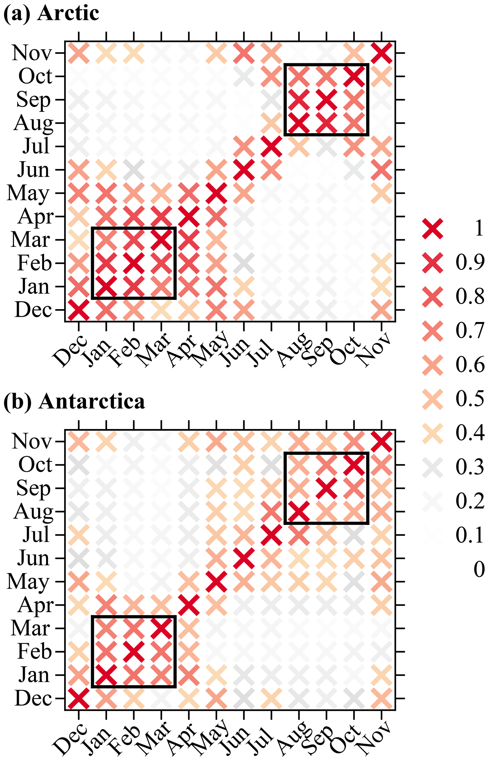
Figure 2Maximum correlation coefficient across the monthly clusters in (a) the Arctic and (b) Antarctica in OSISAF. Two 3-month periods (seasons) stand out with the largest coefficients: January through March (JFM) and August through October (ASO). Values smaller than 1∕e (∼0.37) are considered statistically nonsignificant and plotted in gray. Similar results are obtained using NSIDC and HadISST SIC (and therefore are not shown).
3.2 Sea ice extent
Before comparing SIC clusters, we explore the impact of the ITD discretization on the temporal evolution of the Arctic and Antarctic sea ice extent (SIE) over the period 1979–2014 (Fig. 3). This analysis will help interpret results from the clusters presented later. Note that impacts on the simulated climatological mean state and seasonal cycle over this period have previously been described by Massonnet et al. (2019). In the model, seasonal SIE is calculated from monthly SIC on the original model grid; in observations, seasonal SIE is calculated from the monthly SIE directly provided by the different products. The impact of different ITD discretizations on the Arctic SIE in both seasons and Antarctic SIE in winter is marginal, and all the simulations show values that are within observational uncertainty (which we assume to be defined by the envelope of the different observational products; Fig. 3). The largest differences across simulations are for the summer Antarctic SIE. Increasing the number of categories from 1 to 50 in the S1 discretizations reduces the Antarctic SIE by about 4×10⁶ km2, although the largest decrease, of about 2×10⁶ km2, is between S1.01 and S1.03. This renders the simulated SIE values in the S1 cases closer to those in OSI SAF and NSIDC but further from those in HadISST. HadISST SIE values are consistently above those in OSI SAF and NSIDC in the Arctic and Antarctica in both seasons, as also noted by Titchner and Rayner (2014). Increasing the number of categories in the S2 and S3 discretizations has a comparatively smaller impact, reducing and increasing the summer Antarctic SIE by about 1×10⁶ km2, respectively, yet still within observational uncertainty. The simulated SIE trend is slightly underestimated in the winter Arctic, although it is well captured in summer, as well as in Antarctica in both seasons. In terms of interannual variability, the simulations disagree the most with the observations in Antarctica, especially in summer, when the simulations show large interannual variations that are not found in observations (for example, around 2000). By contrast, the simulated Arctic SIE variability for all ITD discretizations is very close to the observations in both seasons.
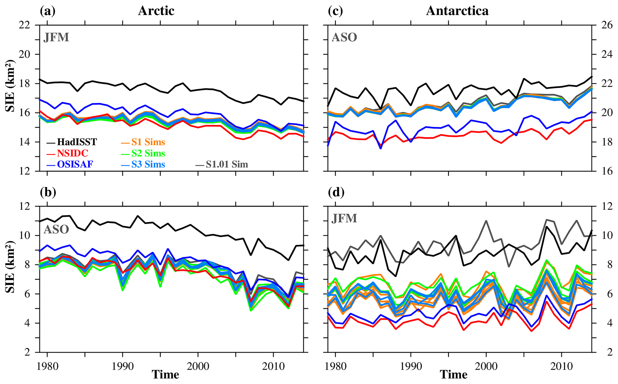
Figure 3(a, b) Arctic and (c, d) Antarctic sea ice extent (SIE; in km2) in (a, d) JFM and (b, c) ASO in the S1, S2, and S3 discretizations (in light red, green, and blue, respectively, with the single-category case, S1.01, in gray) in HadISST, NSIDC, and OSI SAF (in black, blue, and red, respectively). SIE is calculated as the total area of grid cells with concentration larger than 15 %.
To characterize differences between simulated and observed SIC, we calculate the integrated ice edge error (IIEE) as the total area where model and observations disagree on SIC values above 15 % (Goessling et al., 2016). In general terms, the largest IIEE is in the Arctic and Antarctica in winter, with the smallest values when compared with NSIDC (Fig. S1 in the Supplement ). For all the simulations, the IIEE remains relatively constant over the period 1979–2014 at both poles and seasons, and the impact of a different ITD discretization on the IIEE is marginal in the Arctic in both seasons and in Antarctica in winter. The situation is different in the Antarctic summer (JFM), when differences in IIEE due to the ITD are the largest (Fig. 4). IIEE between simulations and observations is overall larger than across observations for all the ITD discretizations. The single-category discretization exhibits the largest IIEE with respect to all observations. Increasing the number of categories in the S1 and S3 cases tends to reduce the IIEE by about 1×10⁶ km2 between the coarsest and finest resolutions. Changes in categories across S2 discretizations have a smaller impact on the IIEE, with no clear improvement or worsening for a finer or coarser ITD. These results suggest that a finer resolution of the thinner ice and not of the thicker sea ice to some degree improves the representation of the simulated Antarctic SIC in winter in our model with respect to observations. This might be related to an improved response of the thin ice (the easiest to melt, grow, and advect) to the atmospheric forcing.

Figure 4Integrated ice edge error (IIEE; in km2) between the Antarctic sea ice in JFM in the (a) S1 (with the case with a single category, S1.01, in gray), (b) S2, and (c) S3 ITD discretizations and in HadISST (dotted lines), NSIDC (dashed lines), and OSISAF (solid lines). Also, IIEE is shown between OSI SAF and NSIDC SIC (gray crosses), NSIDC and HadISST SIC (gray pluses), and HadISST and OSI SAF SIC (gray asterisks). The IIEE is calculated as the integrated area where simulations and observations disagree on SIC above 15 % (Goessling et al., 2016). The darker the color of the line is, the more categories that ITD discretization has. The color scheme matches that in Fig. 1
3.3 SIC cluster analysis
In the following, we describe the three clusters of SIC variability in the observations. Clusters in OSI SAF are shown in Figs. 5 and 6 in the Arctic and Antarctica, respectively (since clusters in NSIDC and HadISST are very similar, they are shown in Figs. S2 and S3, respectively, in the Supplement). In the Arctic winter, the first cluster shows four poles of dominant variability, with more ice in the Barents, Greenland, and Okhotsk seas and less ice in the Labrador and Bering seas (Fig. 5); this pattern agrees with the quadrupole mode described in previous literature associated with variations in the strength of the Siberian High (e.g., Ukita et al., 2007; Close et al., 2017). The second cluster presents similar centers of action to the first one, but SIC anomalies are negative in the Labrador, Barents, and Okhotsk seas and positive in the Bering Sea. The third cluster shows strong anomalies of opposite signs in the Labrador (strongly positive) and Nordic seas (negative), a pattern that resembles the typical fingerprint of a positive NAO phase on the SIC (Bader et al., 2011). In fact, this cluster dominates between 1990 and 1996, when the winter NAO was persistently positive (Hurrell and Deser, 2010). Overall, the first and third clusters alternate until 2004 approximately, after which the second cluster dominates. In the last decade, the root-mean-square distance between the clusters and the anomaly fields (indicated by the symbol size in Fig. 5) increases to its largest values over the whole period in OSI SAF – but not in NSIDC and HadISST. These results suggest that the winter SIC variability might fundamentally have changed after 2004, in agreement with the observed acceleration in the SIC melting trend (e.g., Comiso et al., 2008; Serreze and Stroeve, 2015).
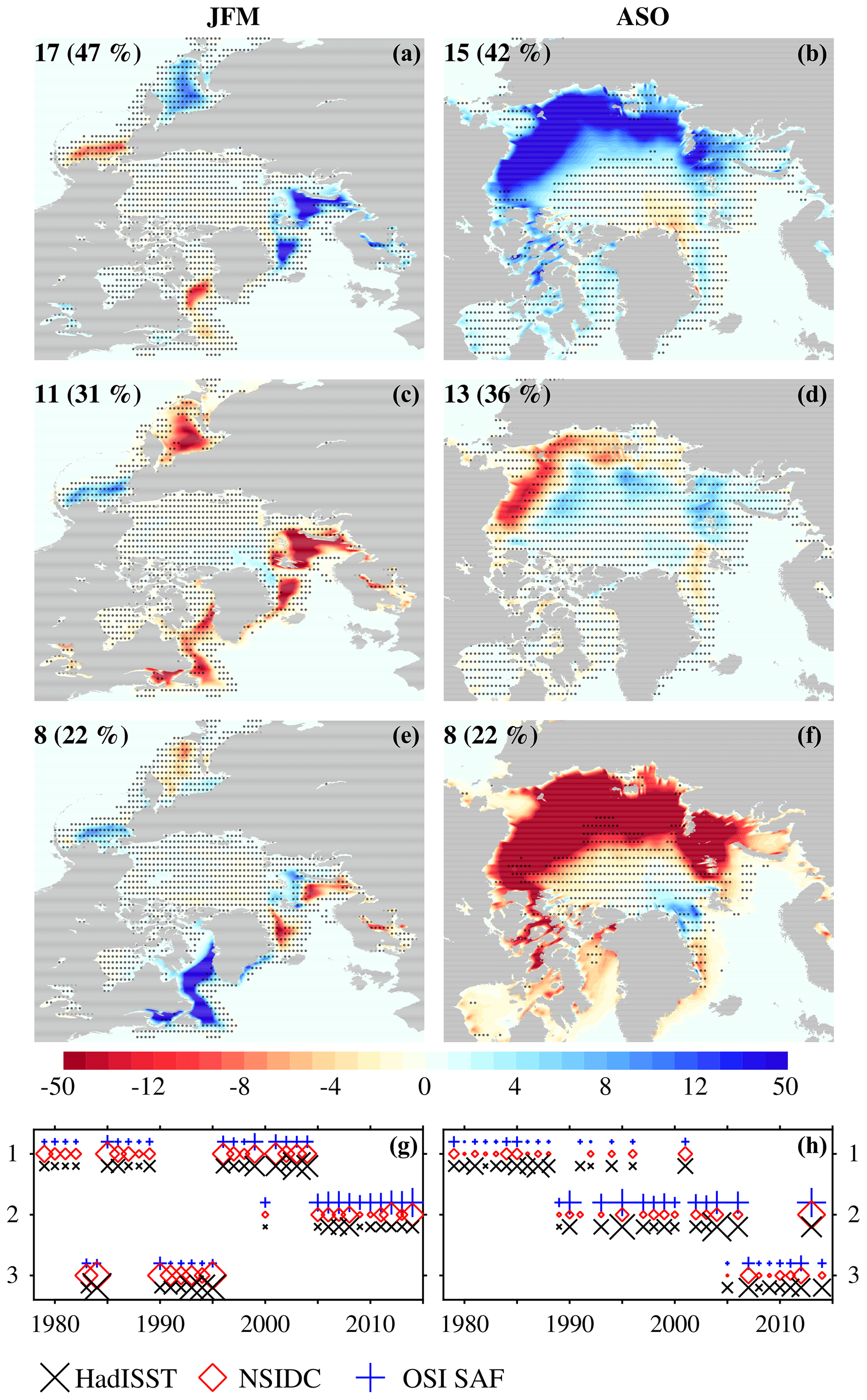
Figure 5(a–f) Cluster patterns of Arctic SIC anomalies (shading; in JFM: a, c, e; and ASO: b, d, f ). Stippling masks statistically nonsignificant anomalies at the 5 % level; p-values at each grid point are computed through a t test that accounts for serial autocorrelation (Manubens et al., 2018). Each cluster's percentage occurrence and the associated number of years whose anomaly pattern explains over the period 1979–2014 is indicated in each case. The shading color scale is adapted for a better view of the anomalies in the range ±15. The area is zoomed in ASO (b, d, f) for a better view of the central Arctic. (g, h) Time series of cluster occurrence in HadISST (black crosses), NSIDC (red diamonds), and OSISAF (blue pluses). The larger the symbol size, the larger the Euclidean distance (root-mean-square difference) between a pattern of anomalies and the associated cluster in a particular year (the maximum symbol size is shown in the legend). Clusters are calculated from the full SIC field without detrending (in contrast to detrended data shown in Fig. 9).
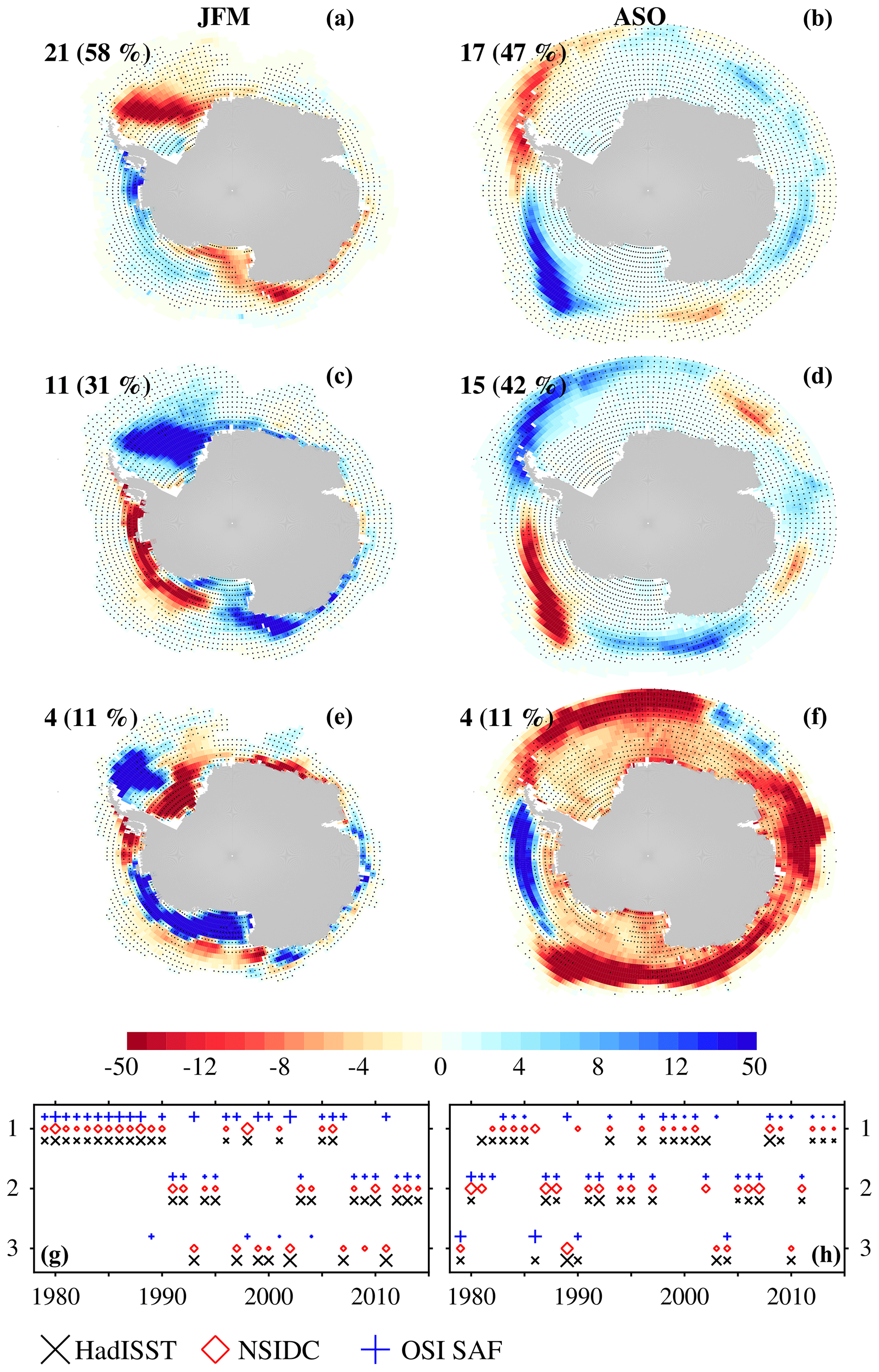
Figure 6As in Fig. 5 but in Antarctica.
In the Arctic summer, both the cluster patterns and relative occurrences reflect a long-term melting trend (Fig. 5). The first and third clusters are very similar: both exhibit widespread positive and negative anomalies in the central Arctic and dominate over the initial period (ca. 1979–1988) and last one (ca. 2005–2014), respectively. The second cluster, by contrast, dominates in the middle decades (ca. 1989–2005) and presents a dipole of positive and negative anomalies between the central Arctic and the surroundings. Such partitioning in decades of alternating dominance suggests that the long-term melting trend in sea ice (as seen in the SIE; Fig. 3b) controls the clustering; previously detrending the data might therefore be necessary for a more robust characterization of the interannual variability (see below).
In the Antarctic summer (JFM), the three clusters exhibit poles of dominant variability close to the continental coast, especially in the Weddell and Ross seas (Fig. 6). The first and second clusters show similar patterns but of opposite sign, with an overall decrease or increase, respectively, but in the Amundsen and Bellinghausen seas. The third cluster shows a dipole with negative anomalies in the Weddell Sea and positive ones in the Amundsen Sea. Summer SIC variability is dominated by the first cluster (58 %), especially during the first decades. Although the second and especially the third clusters are much less frequent (31 % and 11 %, respectively), the second one tends to dominate in the last decade (ca. 2005–2014). This might be due to a slight positive trend, as seen in the SIE (Fig. 3d).
In the Antarctica ASO (winter), the first and second clusters show opposite-sign poles in the Weddell, Bellinghausen, and Amundsen seas, with smaller contributions from the others (Fig. 6). These two modes resemble SIC variability driven by Rossby wave activity across the Drake Passage described in previous literature (e.g., Yuan and Li, 2008; Hobbs and Raphael, 2010; Renwick et al., 2012; Kohyama and Hartmann, 2016). In fact, the first cluster resembles the pattern of Antarctic SIC response to an El Niño (e.g., Ding et al., 2011) and dominates in strong El Niño years, such as 1984, 1998, and 2010. The third cluster shows negative SIC anomalies along all the Antarctic coast but in the Bellingshausen and Amundsen seas, where anomalies are positive; this is however the least persistent cluster (11 %), and SIC variability is clearly dominated by the first two (47 % and 42 %, respectively). Cluster occurrences and patterns in NSIDC are slightly different from those in OSI SAF and HadISTT (Figs. S2 and S3 in the Supplement), suggesting that observational uncertainty impacts the dominant Antarctic SIC modes of variability.
3.3.1 Impact of ITD discretization on the SIC clusters
For each cluster of SIC variability, observations and simulations are compared mainly through their spatial correlation (Fig. 7). Statistical significance of the difference between correlation coefficients is tested using Fisher's z transform, assuming a two-tailed significance level of 0.05 (Storch and Zwiers, 1999). Given the large number of coefficient pairs whose differences can potentially be tested, we simplify the test by comparing only the median values between an ITD discretization and the one immediately below within the same discretization type. For example, S1.50 is compared with S1.30, the latter with S1.10, and so on; S2.15 is compared with S2.11 and so on; and S1.03, S2.03, and S3.05 are all compared with S1.01. As a measure of the observational uncertainty, we also calculate the spatial correlation coefficients between the three observational datasets. We further calculate the root mean square error (RMSE) across observed and simulated clusters to provide an additional assessment. Results of the RMSE analysis are shown in the Arctic only (Fig. S4 in the Supplement ) and are commented when they complement or disagree with results from the spatial correlation coefficients.
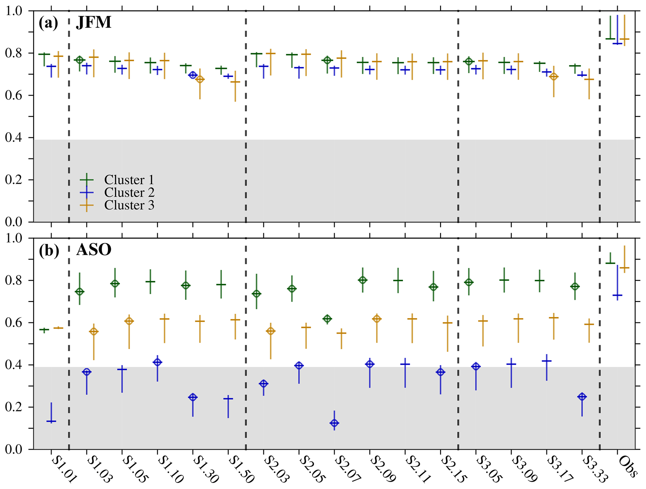
Figure 7Spatial correlation coefficients between the simulated and observed clusters and across the three satellite observational products (marked as Obs) of Arctic SIC in (a) JFM and (b) ASO. For each case, the vertical line spans the maximum and minimum values, and the horizontal line marks the median values; green, blue, and orange lines are for the first, second, and third clusters, respectively. Gray shading masks statistically nonsignificant coefficients below 0.39 value, which corresponds with the minimum value across all the computations that is statistically significant at the 5 % level, accounting for effective degrees of freedom and spatial autocorrelation. A dot is plotted when the difference between the median correlation coefficient values in one discretization and the one immediately below within the same discretization type is statistically significant, based on Fisher's z transform assuming a two-tailed 5 % level. Dashed vertical lines separate between results in the simulation with one single category (S1.01), the different ITD discretizations (S1, S2, and S3), and the observations. Note the discretizations S2.09 and S3.09 are the same (Fig. 1).
In the Arctic winter, correlation coefficients between observed and simulated clusters slightly decrease as the number of categories increases in the three discretization types, and only very few pairs show coefficients that are significantly different (Fig. 7). By contrast, including more categories slightly reduces the RMSE (which suggests a slightly better agreement with the observations) in the third cluster in the S1 and S3 cases and increases it in the S2 one (Fig. S4 in the Supplement ). Overall, nonetheless, changing the ITD discretization has a small impact on model–data agreement, and no discretization or number of categories appears to be consistently the best.
In the Arctic summer, spread in model–data agreement is much larger than in winter (Figs. 7 and S4). The RMSE is barely impacted by the ITD discretization (Fig. S4 in the Supplement ) and shows similar changes to the correlation coefficients. The lowest model–data correlation coefficients are for the second cluster across all discretizations. This is likely because of its characteristic spatial pattern of small, mostly statistically nonsignificant anomalies (Fig. 5). Such noisy features are indeed difficult to accurately capture with the model, thus resulting in comparatively small spatial correlation coefficients. By contrast, anomalies in the first and second clusters take larger values over a larger area and are successfully reproduced by the simulations. Model–data spatial correlation coefficients are little influenced by the ITD discretization for the first and third clusters but show a statistically significant decrease with a number of thin ice categories beyond 30 for the second cluster in the S1 and S3 cases. Although increasing the number of thick categories in the S2 discretization has no major impact on model–data correlation coefficients, the S2.07 case shows a statistically significant drop in correlation values in all the clusters. This suggests that variability is slightly differently distributed across the clusters. The discretization with a single category, S1.01, shows the lowest correlation coefficients (Fig. 7; with statistically significant differences with the coefficients of the S1.03, S2.03, and S3.05 discretizations) and highest RMSE values (Fig. S4 in the Supplement). These results suggest that an ITD with one category or a large number of thin categories hamper representation of SIC variability in the Arctic. This contrasts with and complements results in Massonnet et al. (2019), where the single-category discretization was found performing as good as or even better than multi-category ones in terms of sea ice mean state. Comparison of mass budget across discretizations showed that the single-category case compensates basal ice growth deficit (relative to multi-category cases) through a larger dynamic ice production from fall to winter (and, thus, right for the wrong reasons) (Massonnet et al., 2019).
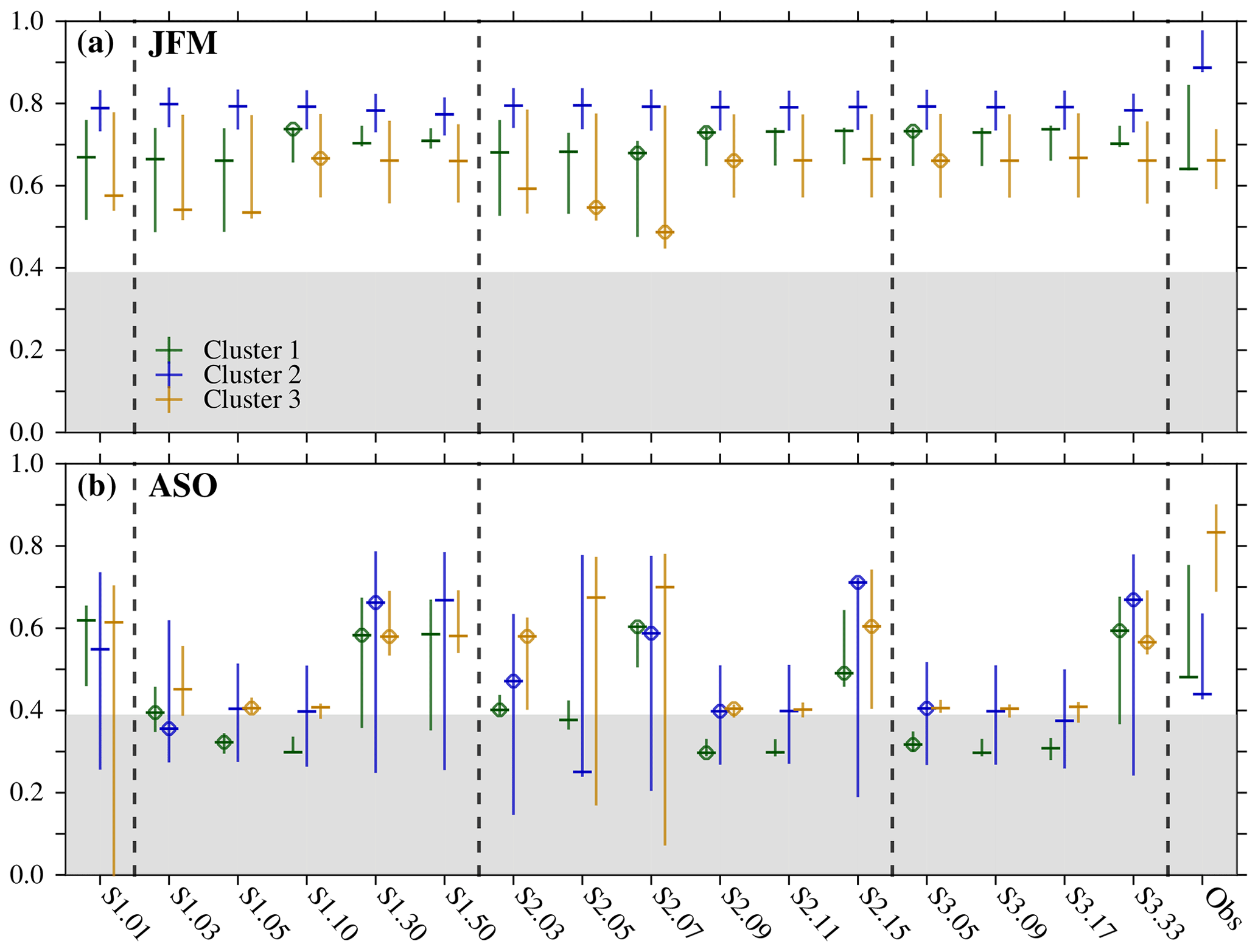
In the Antarctic summer, model–data agreement is lower than in the Arctic in terms of both the spatial correlation (Fig. 8) and RMSE (not shown). Almost all the correlation coefficients are statistically nonsignificant for the second and third cluster (Fig. 8), with only some ITD discretizations with three or five categories showing significant correlations for all clusters. For the first cluster, however, more than five categories show a statistically significant improvement in the agreement with observations, in particular for the S1 cases.
In the Antarctic winter, model–data agreement increases with respect to summer, and correlation coefficients tend to be statistically significant for the first and especially the second cluster (Fig. 8). However, the impact of the ITD distribution is small, and there is no robust response to any discretization.
3.3.2 Arctic SIC clusters after detrending
For a sound characterization of the modes of interannual variability over the period 1979–2014, the long-term, accelerating melting trend in the Arctic SIC is now filtered out. This trend is well captured by both the SIE (Fig. 3) and clusters (Fig. 5). Arctic SIC clusters are now calculated after detrending by removing a spatially varying second-degree polynomial fit with respect to time (see Sect. 2). Clusters calculated after detrending with a first-degree polynomial (linear detrend) are still affected by the melting trend and are not discussed here further. We do not consider higher-degree polynomials either, since they have shown no improvement to characterize clusters of sea ice thickness over the period 1958–2013 (Fučkar et al., 2016). No similar analysis has been performed for Antarctic SIC as the clusters suggest a rather weak positive trend in summer (Fig. 6).
In OSI SAF, detrended SIC variability in winter is evenly distributed into the three clusters (Fig. 9; 36 %, 33 %, and 31 % of occurrence frequency). The first cluster shows a dominant pole of negative anomalies in the Labrador Sea (Fig. 9). The second and third clusters show a similar quadrupole pattern with opposite signs. The second cluster shows two poles of variability in positive and negative anomalies in the Labrador and Nordic seas, respectively. This cluster is very similar to the third one in non-detrended data, and both dominate in similar years with a positive NAO phase. This suggests that they capture the fingerprint of a positive winter NAO on the Arctic SIC. The third cluster is instead similar to the first cluster in the raw data, and both dominate in similar years. They both further resemble the quadrupole pattern analyzed in Close et al. (2017). Clusters in HadISST and NSIDC are very similar and shown in Figs. S4 and S5, respectively, in the Supplement.
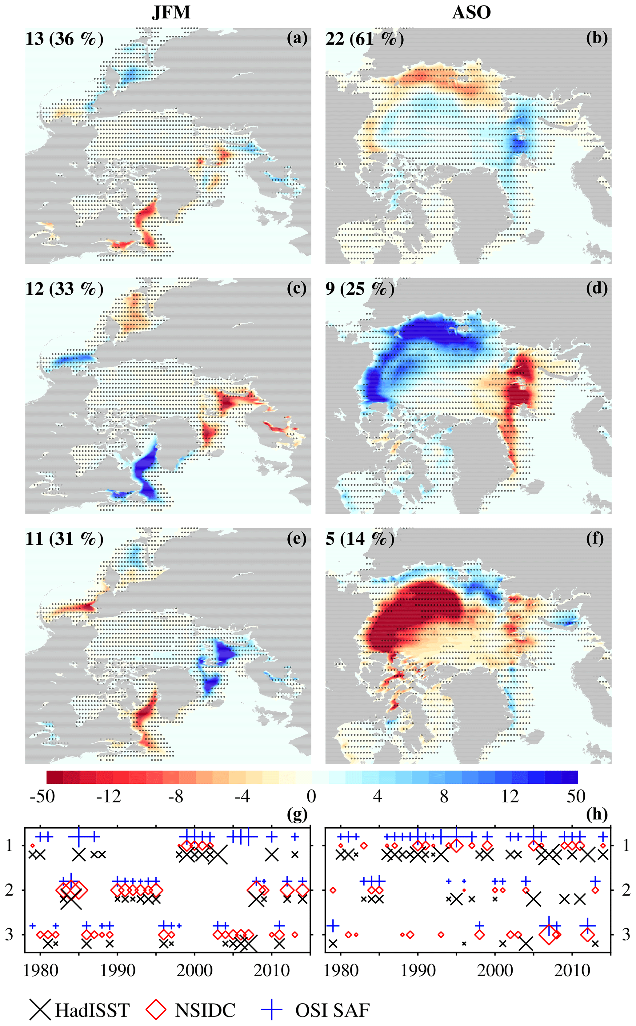
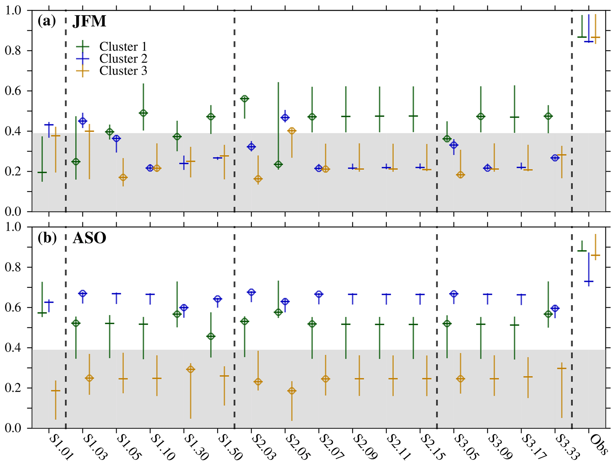
Figure 9As in Fig. 5 but after detrending with a second-degree polynomial.
In summer, detrending the data leads to clusters with more marked regional contrasts (compare Figs. 5 and 9). The first cluster in OSI SAF, which dominates in two-thirds of the years, shows a dipole of positive SIC anomalies in the Kara, Barents, and Greenland seas and negative ones in the East Siberian and Laptev seas (Fig. 9). The second cluster mirrors the first one but with opposite-sign and larger anomalies (Fig. 9). These two clusters, respectively, resemble the fingerprint of a positive (in 1995, 1999, 2002, and 2005) and negative (in 1996 and 2004) Arctic dipole on the summer SIC (Wang et al., 2009). Occurrence of these two clusters, however, does not systematically coincide with strong Arctic dipole anomalies (for example, in 1998 or 2003; Wang et al., 2009). The Arctic oscillation has also been proposed as a driver of similar SIC anomaly patterns (Rigor et al., 2002; Rigor and Wallace, 2004; Wang et al., 2009). Lastly, the third cluster shows a monopole of strong negative anomalies confined to the Beaufort Gyre. This pattern dominates only in 4 years, including 2007, when the Arctic sea ice extent was the lowest over the period 1979–2014. Extreme melting events such that have been associated with exceptional episodes of atmospheric (Graversen et al., 2011) and oceanic (Woodgate et al., 2010) warm flow into polar latitudes and summer storm activity (Screen et al., 2011). Note that cluster repartitioning of detrended data is not exactly the same as in HadISST and NSIDC in summer (Fig. S5 in the Supplement ); their first clusters are similar to the first one in OSI SAF but with different local expressions; their third clusters resemble the second one in OSI SAF but with weaker anomalies near the Alaskan coast.
With respect to the sensitivity of the model clusters to the ITD discretization, we find that the winter clusters rather consistently agree with the observed ones both in terms of the spatial correlation coefficients (Fig. 10) and RMSE (not shown) and are little impacted by the discretization. In summer, increasing the number of categories beyond 30 leads to a statistically significant improvement in model–data correlation coefficients (Fig. 10), while reducing the RMSE (not shown) for all the clusters in the S1 and S3 discretizations. This implies that, overall, a large number of thin categories help improve the representation of SIC interannual variability in summer. In contrast to what happens in non-detrended data, the single-category discretization agrees with the observations as well as any other. This suggests that one category poorly captures the forced variability (this is, the long-term melting trend) but is as good as any other discretization at capturing interannual variability.
3.4 Anomaly-based analyses
Two extra analyses are discussed in the following to complement previous ones and explore their robustness. In the first analysis, spatial correlation coefficients are computed directly, in each year, between the simulated and observed SIC anomalies in both seasons and hemispheres. In each case, a distribution of correlation coefficients is generated by combining the values in all the years and in the three observational products. This analysis suggests only marginal sensitivity to the number of sea ice categories or its discretization in the Arctic before (Fig. S6 in the Supplement) and after detrending (not shown) and in Antarctica (not shown).
The second analysis provides a spatial perspective on the impacts of the ITD discretizations on SIC. For this, temporal correlation coefficients at the grid point level are first computed between simulated and observed SIC anomalies in both seasons. A linear fit of such correlation coefficients with respect to the number of categories is then calculated across simulations of a given discretization. The result is a map which provides a measure of the regions where changing the number of categories most impacts agreement with observations. Since results are similar across the observational products, an average between the three cases is computed for the Arctic (Fig. 11) and Antarctica (Fig. S7 in the Supplement).
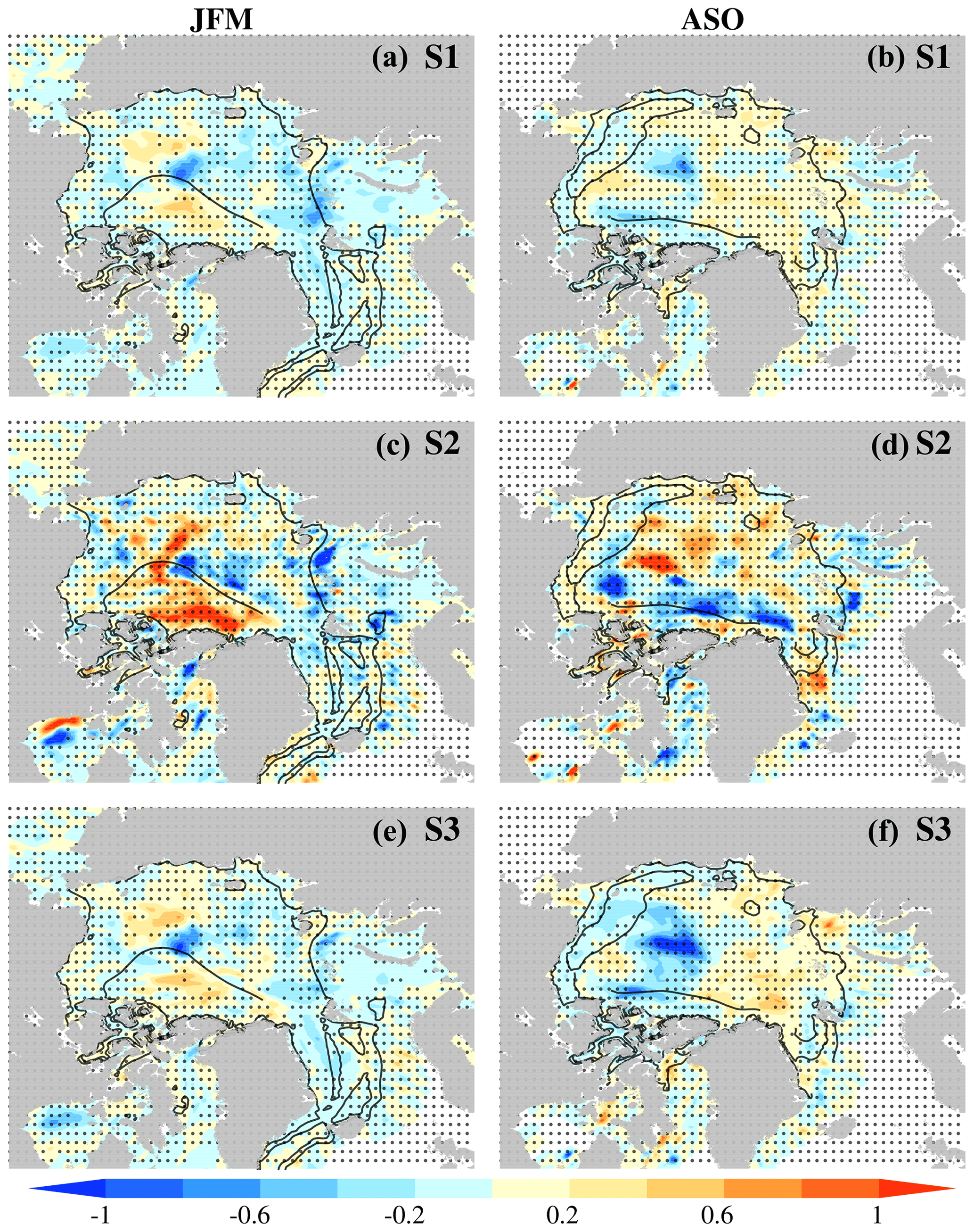
Figure 11Trend relative to the number of sea ice categories in pointwise temporal correlation coefficients between simulated and observed Arctic SIC anomalies (in [number of categories]−1) in the (a, b) S1, (c, d) S2, and (e, f) S3 discretizations in (a, c, e) JFM and (b, d, f) ASO. An average between results in OSI SAF, NSIDC, and HadISST is shown. Values are multiplied by 100 to ease the interpretation and the color shading is adapted for a better view of the values between −1 and 1. A value of 0.5, for example, indicates that the model–data correlation coefficient increases 0.5 when the number of categories increases by 100 (or 0.25 for an increase of 50 categories). Stippling masks trend values which are statistically nonsignificant at the 5 % level based on a two-tailed Student's t test. Contours are the simulated climatological ice thickness (every 1.5 m) in the standard LIM3 discretization of five categories (S1.05) for the period 1979–2014.
Increasing the number of categories tends to decrease model–data agreement (blue colors in Fig. 11) in the S1 and S3 discretizations in both seasons (but most clearly in the S3 one in summer) in the central Arctic, near the region where the largest increase in sea ice thickness is simulated for an increase in the number of categories (Massonnet et al., 2019). In this region, a larger bottom growth rate increases the sea ice volume for finer ITD resolutions. This is because conductive heat flux through ice, which is inversely proportional to ice thickness, increases (facilitates ice growth) on average on a grid cell when the thickest ice accumulates on a few categories and thereby leaves more grid space for faster-growing thin ice (Massonnet et al., 2019). In the central Arctic, therefore, higher sea ice volume makes the simulated sea ice less realistic. In the S2 discretizations, model–data agreement particularly improves with the number of categories in winter north off Greenland and the Queen Elizabeth Islands, regions where the thickest ice is simulated (Fig. 11, contours). Although the overall Arctic sea ice volume increases with the number of categories (Massonnet et al., 2019), the improvement in that particular region suggests that a discretization including more thick categories helps capture variability in thick ice. In summer, a decrease in model–data agreement occurs in the same region, although there are improvements elsewhere in the central Arctic that might compensate for this decrease (Fig. 11). In Antarctica, only the S2 discretization in summer (JFM) shows some clear trends in model–data agreement near the Ross Sea (Fig. S7 in the Supplement). However, these results appear spurious as sea ice is very thin and presents a concentration below 15 % in the area (contours in Fig. S7 in the Supplement).
This article explores the impact of different ITD discretizations on the simulated SIC variability in the Arctic and Antarctica. Using ocean–sea ice stand-alone simulations with the NEMO3.6—LIM3 model, we assess three different ITD discretizations in which both the number and boundaries of the sea ice thickness categories are changed. SIC variability is characterized via K-means clustering analysis over the period 1979–2014; the simulated clusters are compared with those from three satellite observational products, OSI SAF, NSIDC, and HadISST v2.2. We focus on two seasons, JFM (winter) and ASO (summer), across which monthly clusters are found most spatially coherent. In the Arctic, cluster comparison is done by including and excluding the long-term trend, the latter by detrending with a spatially varying second-degree polynomial. We complement the cluster analysis by comparing sea ice extent and anomaly fields between model and observations.
Overall, winter clusters reflect the imprint of atmospheric variability such as the NAO and Siberian High on the Arctic SIC and that of ENSO on the Antarctic SIC. Summer clusters reflect the dominant trends in SIC, slightly positive in Antarctica and prominently negative in the Arctic. After detrending, Arctic summer clusters allow isolation of the SIC response to atmospheric variability associated with the Arctic Dipole and Arctic Oscillation, as well as identifying outstanding events such as the 2007 sea ice extent minimum.
Although the results of all the model–data comparisons present mixed conclusions, depending on the analysis, we extract a few take-home messages:
- i.
The single-category discretization shows the worst results overall, particularly in the Arctic summer without detrending due to a misrepresentation of the long-term melting trend. This result reinforces the recommendation of using multi-category sea ice models. In the companion study, Massonnet et al. (2019), the single-category discretization is found producing realistic mean states of sea ice extent; it was however hypothesized that this might be for the wrong reasons, thanks to error compensation in the simulated mass balance terms. The finding of the present study, focusing on variability, supports that the single-category framework is in fact not appropriate for investigating the cause of large-scale sea ice changes.
- ii.
Discretizations with more than 10 sea ice thickness categories can degrade model ability to simulate realistic Arctic SIC variability. In particular, better resolving thin ice in the Arctic hampers SIC representation, likely related to an unrealistic sea ice volume increase in the central Arctic (Massonnet et al., 2019) and a poorer representation of the long-term melting trend in summer (this study). In contrast, a finer resolution in thin sea ice increases realism of the simulated SIC in Antarctica; this improvement, nonetheless, most clearly arises for more than 30 thin categories, for which computational costs increase substantially (from 30 min per simulated year for the standard five-category discretization to 60 min for the 30-category one; Massonnet et al., 2019). With respect to including more thick categories, our analysis shows that it improves variability in very thick sea ice north of Greenland in winter without noticeably compromising the performance in other regions or in summer.
That multiple-category discretizations can degrade model realism appears counterintuitive, since a finer resolution should allow the sea ice model to reproduce actual subgrid-scale variability in sea ice better. We note, however, that NEMO3.6–LIM3 uses parametrizations and parameter values which are adjusted for the five-category discretization. Adjustments in the ITD may therefore need retuning those parametrizations and parameter values, which in LIM3 include, among others, the snow thermal conductivity, the bare sea-ice albedo, and the compressive ice strength, P*. Such model retuning is however beyond our scope, as improvements in SIC variability would hence result from the new model setup and not from each different ITD discretization.
Since no robust conclusion about the optimal number of sea ice categories can be drawn based on our analyses, we recommend using the standard (S1.05) or a similar discretization in NEMO3.6–LIM3, which is, in addition, computationally more efficient than others with more categories. This is in line with previous studies finding that discretizations with five to seven categories represent sea ice characteristics realistically enough (Bitz et al., 2001; Lipscomb, 2001; Massonnet et al., 2019). As noted by Hunke (2014), however, in the Los Alamos Sea Ice Model CICE “5 ice thickness categories are not enough to accurately represent observed thickness data nor to properly model mechanical sea ice processes that control ice volume”.
A growing number of climate models now include a sea ice model with an ITD, such as LIM3, the Los Alamos Sea Ice Model CICE (Hunke et al., 2013), and the GFDL's SIS2.0 (Adcroft et al., 2019), and the prospect is that more will do so in the future. Although including an ITD has been proven to be beneficial for simulating more realistic sea ice characteristics (e.g., Bitz et al., 2001; Holland et al., 2006; Massonnet et al., 2011; Ungermann et al., 2017; Uotila et al., 2017), it introduces potential new tuning options, such as the number of categories, their boundaries, and the assumed shape function, which might need further validation against observations. A very fine ITD also makes simulation computationally very expensive, a factor that is particularly limiting in fully coupled models. Similar analyses to the one presented here would therefore be necessary to assess the impact of using a specific ITD discretization in a particular climate model. The extent to which our particular recommendation for NEMO3.6–LIM3 can be extended to other sea ice models is difficult to assess, however, considering that new tuning might be necessary for each ITD discretization, and that different sea ice models might have different tuning parameters and sensitivity to their values.
A potential caveat of our study is the use of ocean stand-alone simulations. These are aimed to reduce potential uncertainty sources in SIC variability associated with stochastic atmospheric noise, which might mask comparison with observations and the search for improvements in model realism. An open question for future studies is then whether our conclusions would hold in coupled model configurations, where ice–atmosphere feedbacks might modulate the influence of ITD discretization. We propose an analysis focused on the impacts on sea ice and surface energy flux seasonal cycles, variability modes, and long-term trends, similar to this study and its companion paper, Massonnet et al. (2019). The cost and benefits of such an analysis in coupled setups should however be weighted carefully beforehand, considering the limited impacts we find in ocean stand-alone simulations and the increase in computational costs for ITD discretizations with large numbers of categories.
This study and its companion, Massonnet et al. (2019), present an advance with respect to previous efforts since they jointly address the response of the mean climatological state and variability in sea ice to changes in a model parametrization. This approach sets an example for future assessments of the impact of model parametrizations on the representation of the sea ice or other climatic variables. Unfortunately, observational data are still too short for many climate components, making this sort of analysis particularly challenging at best.
The model source code is available at https://doi.org/10.5281/zenodo.3345604 (Massonnet, 2019). Data and code to reproduce the authors' work can be obtained from https://doi.org/10.5281/zenodo.3540756 (Moreno-Chamarro et al., 2019).
The supplement related to this article is available online at: https://doi.org/10.5194/gmd-13-4773-2020-supplement.
EMC and PO conceived the study. FM provided the model data. EMC analyzed the model and observational data and wrote the paper with contributions from all authors. All authors contributed to interpreting the results.
The authors declare that they have no conflict of interest.
Computational resources have been provided by the supercomputing facilities of the Université catholique de Louvain (CISM/UCL) and the Consortium des Equipements de Calcul Intensif en Fédération Wallonie Bruxelles (CECI) funded by the F.R.S.-FNRS under convention 2.5020.11. François Massonnet is a F.R.S.-FNRS Research Associate.
This research has been supported by the European Commission's Horizon 2020 APPLICATE project (grant no. GA 727862) and the European Commission's Horizon 2020 PRIMAVERA project (grant no. GA 641727).
This paper was edited by Olivier Marti and reviewed by two anonymous referees.
Adcroft, A., Anderson, W., Balaji, V., Blanton, C., Bushuk, M., Dufour, C. O., Dunne, J. P., Griffies, S. M., Hallberg, R., Harrison, M. J., and Held, I. M.: The GFDL global ocean and sea ice model OM4.0: Model description and simulation features, J. Adv. Model. Earth Sy., 11, 3167–3211, https://doi.org/10.1029/2019MS001726, 2019.
Anderberg, M. R.: Cluster analysis for applications: probability and mathematical statistics: a series of monographs and textbooks, vol. 19, Academic Press, London, 2014.
Bader, J., Mesquita, M. D., Hodges, K. I., Keenlyside, N., Østerhus, S., and Miles, M.: A review on Northern Hemisphere sea-ice, storminess and the North Atlantic Oscillation: Observations and projected changes, Atmos. Res., 101, 809–834, https://doi.org/10.1016/j.atmosres.2011.04.007, 2011
Barthélemy, A., Goosse, H., Fichefet, T., and Lecomte, O.: On the sensitivity of Antarctic sea ice model biases to atmospheric forcing uncertainties, Clim. Dynam., 51, 1–19, https://doi.org/10.1007/s00382-017-3972-7, 2018.
Bitz, C. M., Holland, M. M., Weaver, A. J., and Eby, M.: Simulating the ice-thickness distribution in a coupled climate model, J. Geophys. Res.-Oceans, 106, 2441–2463, https://doi.org/10.1029/1999JC000113, 2001.
Blackport, R., Screen, J. A., van der Wiel, K., and Bintanja, R.: Minimal influence of reduced Arctic sea ice on coincident cold winters in mid-latitudes, Nat. Clim. Change, 9, 697–704, https://doi.org/10.1038/s41558-019-0551-4, 2019.
Brodeau, L., Barnier, B., Treguier, A. M., Penduff, T., and Gulev, S.: An ERA40-based atmospheric forcing for global ocean circulation models, Ocean Model., 31, 88–104, https://doi.org/10.1016/j.ocemod.2009.10.005, 2010.
Cavalieri, D. J., Parkinson, C. L., Gloersen, P., and Zwally, H. J.: Sea ice concentrations from Nimbus-7 SMMR and DMSP SSM/I-SSMIS passive microwave data, version 1, National Snow and Ice Data Center, Boulder, CO, USA, 1996.
Charrad, M., Ghazzali, N., Boiteau, V., and Niknafs, A.: NbClust: An R Package for Determining the Relevant Number of Clusters in a Data Set, J. Stat. Softw., 61, 1–36, https://doi.org/10.18637/jss.v061.i06, 2014.
Close, S., Houssais, M. N., and Herbaut, C.: The Arctic winter sea ice quadrupole revisited, J. Climate, 30, 3157–3167, https://doi.org/10.1175/JCLI-D-16-0506.1, 2017.
Coggins, J. H., McDonald, A. J., and Jolly, B.: Synoptic climatology of the Ross Ice Shelf and Ross Sea region of Antarctica: k-means clustering and validation, Int. J. Climatol., 34, 2330–2348, https://doi.org/10.1002/joc.3842, 2014.
Comiso, J. C., Parkinson, C. L., Gersten, R., and Stock, L.: Accelerated decline in the Arctic sea ice cover, Geophys. Res. Lett., 35, L01703, https://doi.org/10.1029/2007GL031972, 2008.
Dai, A. and Trenberth, K. E.: Estimates of freshwater discharge from continents: Latitudinal and seasonal variations, J. Hydrometeorol., 3, 660–687, https://doi.org/10.1175/1525-7541(2002)003<0660:EOFDFC>2.0.CO;2, 2002.
Day, J. J., Hargreaves, J. C., Annan, J. D., and Abe-Ouchi, A.: Sources of multi-decadal variability in Arctic sea ice extent, Environ. Res. Lett., 7, 034011, https://doi.org/10.1088/1748-9326/7/3/034011, 2012.
Delworth, T. L., Zeng, F., Vecchi, G. A., Yang, X., Zhang, L., and Zhang, R.: The North Atlantic Oscillation as a driver of rapid climate change in the Northern Hemisphere, Nat. Geosci., 9, 509–512, https://doi.org/10.1038/ngeo2738, 2016.
Depoorter, M. A., Bamber, J. L., Griggs, J. A., Lenaerts, J. T. M., Ligtenberg, S. R., Van den Broeke, M. R., and Moholdt, G.: Calving fluxes and basal melt rates of Antarctic ice shelves, Nature, 502, 89–92, https://doi.org/10.1038/nature12567, 2013.
Ding, Q., Steig, E. J., Battisti, D. S., and Küttel, M. Winter warming in West Antarctica caused by central tropical Pacific warming, Nat. Geosci., 4, 398–403, https://doi.org/10.1038/ngeo1129, 2011.
Drinkwater, K. F., Miles, M., Medhaug, I., Otterå, O. H., Kristiansen, T., Sundby, S., and Gao, Y.: The Atlantic Multidecadal Oscillation: Its manifestations and impacts with special emphasis on the Atlantic region north of 60 N, J. Marine Syst., 133, 117–130, https://doi.org/10.1016/j.jmarsys.2013.11.001, 2014.
Dussin, R., Barnier, B., Brodeau, L., and Molines, J.-M.: The making of the DRAKKAR Forcing Set DFS5, Drakkar/myocean report 01-04-16, Laboratoire de Glaciologie et de Géophysique de l’Environnement, Université de Grenoble, Grenoble, France, available at: https://www.drakkar-ocean.eu/forcing-the-ocean (last access: 19 August 2019), 2016
EUMETSAT Ocean and Sea Ice Satellite Application Facility: Global sea ice concentration reprocessing dataset 1978–2015 (v1.2), Norwegian and Danish Meteorological Institutes, available at: https://catalogue.ceda.ac.uk/uuid/8bbde1a8a0ce4a86904a3d7b2b917955 (last access: 23 September 2015), 2015.
Fučkar, N. S., Guemas, V., Johnson, N. C., Massonnet, F., and Doblas-Reyes, F. J.: Clusters of interannual sea ice variability in the northern hemisphere, Clim. Dynam., 47, 1527–1543, https://doi.org/10.1007/s00382-015-2917-2, 2016.
Fučkar, N. S., Guemas, V., Johnson, N. C., and Doblas-Reyes, F. J.: Dynamical prediction of Arctic sea ice modes of variability, Clim. Dynam., 52, 1–17, https://doi.org/10.1007/s00382-018-4318-9, 2018.
Goessling, H. F., Tietsche, S., Day, J. J., Hawkins, E., and Jung, T.: Predictability of the Arctic sea ice edge, Geophys. Res. Lett., 43, 1642–1650, https://doi.org/10.1002/2015GL067232, 2016.
Graversen, R. G., Mauritsen, T., Drijfhout, S., Tjernström, M., and Mårtensson, S.: Warm winds from the Pacific caused extensive Arctic sea-ice melt in summer 2007, Clim. Dynam., 36, 2103–2112, https://doi.org/10.1007/s00382-010-0809-z, 2011.
Hastie, T., Tibshirani, R., and Friedman, J.: The elements of statistical learning: data mining, inference, and prediction, Springer Series in Statistics, Springer New York, NY, https://doi.org/10.1007/978-0-387-84858-7, 2009.
Hibler, W. D: Ice dynamics, in: The Geophysics of Sea Ice, Springer, Boston, MA, 577–640, https://doi.org/10.1007/978-1-4899-5352-0_10, 1986.
Hobbs, W. R. and Raphael, M. N.: The Pacific zonal asymmetry and its influence on Southern Hemisphere sea ice variability, Antarctic Sci., 22, 559–571, https://doi.org/10.1017/S0954102010000283, 2010.
Holland, M. M., Bitz, C. M., Hunke, E. C., Lipscomb, W. H., and Schramm, J. L.: Influence of the sea ice thickness distribution on polar climate in CCSM3, J. Climate, 19, 2398–2414, https://doi.org/10.1175/JCLI3751.1, 2006.
Holland, P. R. and Kwok, R.: Wind-driven trends in Antarctic sea-ice drift, Nat. Geosci., 5, 872–875, https://doi.org/10.1038/ngeo1627, 2012.
Hunke, E. C.: Sea ice volume and age: Sensitivity to physical parameterizations and thickness resolution in the CICE sea ice model, Ocean Model., 82, 45–59, https://doi.org/10.1016/j.ocemod.2014.08.001, 2014.
Hunke, E. C., Lipscomb, W. H., Turner, A. K., Jeffery, N., and Elliott, S.: CICE: the Los Alamos Sea Ice Model, Documentation and Software User's Manual, version 5.0., Technical Report LA-CC-06-012, Los Alamos National Laboratory, Los Alamos, New Mexico, 2013.
Hurrell, J. W., and Deser, C.: North Atlantic climate variability: the role of the North Atlantic Oscillation, J. Marine Syst., 79, 231–244, https://doi.org/10.1016/j.jmarsys.2009.11.002, 2010
Ingvaldsen, R. B., Asplin, L., and Loeng, H.: The seasonal cycle in the Atlantic transport to the Barents Sea during the years 1997–2001, Cont. Shelf Res., 24, 1015–1032, https://doi.org/10.1016/j.csr.2004.02.011, 2004a.
Ingvaldsen, R. B., Asplin, L., and Loeng, H.: Velocity field of the western entrance to the Barents Sea, J. Geophys. Res.-Oceans, 109, C03021, https://doi.org/10.1029/2003JC001811, 2004b.
Kohyama, T. and Hartmann, D. L.: Antarctic sea ice response to weather and climate modes of variability, J. Climate, 29, 721–741, https://doi.org/10.1175/JCLI-D-15-0301.1, 2016.
Large, W. G., and Yeager, S. G. Diurnal to decadal global forcing for ocean and sea-ice models: the data sets and flux climatologies, NCAR Technical Note, National Center for Atmospheric Research, 11, 324–336, 2004.
Laxon, S. W., Giles, K. A., Ridout, A. L., Wingham, D. J., Willatt, R., Cullen, R., Kwok, R., Schweiger, A., Zhang, J., Haas, C., and Hendricks, S.: CryoSat-2 estimates of Arctic sea ice thickness and volume, Geophys. Res. Lett., 40, 732–737, https://doi.org/10.1002/grl.50193, 2013.
Lipscomb, W. H.: Remapping the thickness distribution in sea ice models, J. Geophys. Res.-Oceans, 106, 13989–14000, https://doi.org/10.1029/2000JC000518, 2001.
Lynch, A. H., Serreze, M. C., Cassano, E. N., Crawford, A. D., and Stroeve, J.: Linkages between Arctic summer circulation regimes and regional sea ice anomalies, J. Geophys. Res.-Atmos., 121, 7868–7880, https://doi.org/10.1002/2016JD025164, 2016.
Madec, G.: NEMO ocean engine, Note du Pole de modélisation, Institut Pierre-Simon Laplace (IPSL), France, No. 27, ISSN 1288–1619, 2008.
Manubens, N., Caron, L. P., Hunter, A., Bellprat, O., Exarchou, E., Fučkar, N. S., Garcia-Serrano, J., Massonnet, F., Ménégoz, M., Sicardi, V., and Batté, L.: An R package for climate forecast verification, Environ. Modell. Softw., 103, 29–42, 2018.
Massonnet, F.: fmassonn/paper-itd-seaice: Accepted paper (Version 1.2.0), Zenodo, https://doi.org/10.5281/zenodo.3345604, 2019.
Massonnet, F., Fichefet, T., Goosse, H., Vancoppenolle, M., Mathiot, P., and König Beatty, C.: On the influence of model physics on simulations of Arctic and Antarctic sea ice, Cryosphere, 5, 687–699, https://doi.org/10.5194/tc-5-687-2011, 2011.
Massonnet, F., Barthélemy, A., Worou, K., Fichefet, T., Vancoppenolle, M., Rousset, C., and Moreno-Chamarro, E.: On the discretization of the ice thickness distribution in the NEMO3.6-LIM3 global ocean–sea ice model, Geosci. Model Dev., 12, 3745–3758, https://doi.org/10.5194/gmd-12-3745-2019, 2019.
Maykut, G. A. and Untersteiner, N.: Some results from a time-dependent thermodynamic model of sea ice, J. Geophys. Res., 76, 1550–1575, https://doi.org/10.1029/JC076i006p01550, 1971.
Merino, N., Le Sommer, J., Durand, G., Jourdain, N. C., Madec, G., Mathiot, P., and Tournadre, J.: Antarctic icebergs melt over the Southern Ocean: Climatology and impact on sea ice, Ocean Model., 104, 99–110, https://doi.org/10.1016/j.ocemod.2016.05.001, 2016.
Michelangeli, P. A., Vautard, R., and Legras, B.: Weather regimes: Recurrence and quasi stationarity, J. Atmos. Sci., 52, 1237–1256, https://doi.org/10.1175/1520-0469(1995)052<1237:WRRAQS>2.0.CO;2, 1995.
Miles, M. W., Divine, D. V., Furevik, T., Jansen, E., Moros, M., and Ogilvie, A. E.: A signal of persistent Atlantic multidecadal variability in Arctic sea ice, Geophys. Res. Lett., 41, 463–469, https://doi.org/10.1002/2013GL058084, 2014.
Moreno-Chamarro, E., Ortega, P., and Massonnet, F.: Impact of the ice thickness distribution discretization on the sea ice concentration variability in the NEMO3.6-LIM3 global ocean–sea ice model (Version 1.0) [Data set], Geoscientific Model Development, Zenodo, https://doi.org/10.5281/zenodo.3540757, 2019.
Ogi, M. and Wallace, J. M.: Summer minimum Arctic sea ice extent and the associated summer atmospheric circulation, Geophys. Res. Lett., 34, L12705, https://doi.org/10.1029/2007GL029897, 2007.
Olonscheck, D., Mauritsen, T., and Notz, D.: Arctic sea-ice variability is primarily driven by atmospheric temperature fluctuations, Nat. Geosci., 12, 430–434, https://doi.org/10.1038/s41561-019-0363-1, 2019.
Renwick, J. A., Kohout, A., and Dean, S.: Atmospheric forcing of Antarctic sea ice on intraseasonal time scales, J. Climate, 25, 5962–5975, https://doi.org/10.1175/JCLI-D-11-00423.1, 2012.
Rigor, I. G., Wallace, J. M., and Colony, R. L.: Response of sea ice to the Arctic Oscillation, J. Climate, 15, 2648–2663, https://doi.org/10.1175/1520-0442(2002)015<2648:ROSITT>2.0.CO;2, 2002.
Rigor, I. G. and Wallace, J. M.: Variations in the age of Arctic sea-ice and summer sea-ice extent. Geophys. Res. Lett., 31, L09401, https://doi.org/10.1029/2004GL019492, 2004.
Rossow, W. B., Tselioudis, G., Polak, A., and Jakob, C.: Tropical climate described as a distribution of weather states indicated by distinct mesoscale cloud property mixtures. Geophys. Res. Lett., 32, L21812, https://doi.org/10.1029/2005GL024584, 2005.
Rousset, C., Vancoppenolle, M., Madec, G., Fichefet, T., Flavoni, S., Barthélemy, A., Benshila, R., Chanut, J., Levy, C., Masson, S., and Vivier, F.: The Louvain-La-Neuve sea ice model LIM3.6: global and regional capabilities, Geosci. Model Dev., 8, 2991–3005, https://doi.org/10.5194/gmd-8-2991-2015, 2015.
Schlichtholz, P.: Influence of oceanic heat variability on sea ice anomalies in the Nordic Seas, Geophys. Res. Lett., 38, L05705, https://doi.org/10.1029/2010GL045894, 2011.
Screen, J. A.: Influence of Arctic sea ice on European summer precipitation, Environ. Res. Lett., 8, 044015, https://doi.org/10.1088/1748-9326/8/4/044015, 2013.
Screen, J. A., Simmonds, I., and Keay, K.: Dramatic interannual changes of perennial Arctic sea ice linked to abnormal summer storm activity, J. Geophys. Res.-Atmos., 116, D15105, https://doi.org/10.1029/2011JD015847, 2011.
Serreze, M. C. and Stroeve, J.: Arctic sea ice trends, variability and implications for seasonal ice forecasting, Philos. T. R. Soc. A, 373, 20140159, https://doi.org/10.1098/rsta.2014.0159, 2015.
Sonnewald, M., Wunsch, C., and Heimbach, P.: Unsupervised learning reveals geography of global ocean dynamical regions, Earth Space Sci., 6, 784–794, https://doi.org/10.1029/2018EA000519, 2019.
Storch, H. and Zwiers, F.: Statistical analysis in climate research, Cambridge University Press, Cambridge, https://doi.org/10.1017/CBO9780511612336, 1999.
Thorndike, A. S., Rothrock, D. A., Maykut, G. A., and Colony, R.: The thickness distribution of sea ice, J. Geophys. Res., 80, 4501–4513, https://doi.org/10.1029/JC080i033p04501, 1975.
Titchner, H. A. and Rayner, N. A.: The Met Office Hadley Centre sea ice and sea surface temperature data set, version 2: 1. Sea ice concentrations, J. Geophys. Res.-Atmos, 119, 2864–2889, https://doi.org/10.1002/2013JD020316, 2014.
Ukita, J., Honda, M., Nakamura, H., Tachibana, Y., Cavalieri, D. J., Parkinson, C. L., Koide, H., and Yamamoto, K.: Northern Hemisphere sea ice variability: Lag structure and its implications, Tellus A, 59, 261–272, https://doi.org/10.1111/j.1600-0870.2006.00223.x, 2007.
Ungermann, M., Tremblay, L. B., Martin, T., and Losch, M.: Impact of the ice strength formulation on the performance of a sea ice thickness distribution model in the Arctic, J. Geophys. Res.-Oceans, 122, 2090–2107, https://doi.org/10.1002/2016JC012128, 2017.
Uotila, P., Iovino, D., Vancoppenolle, M., Lensu, M., and Rousset, C.: Comparing sea ice, hydrography and circulation between NEMO3.6 LIM3 and LIM2, Geosci. Model Dev., 10, 1009–1031, https://doi.org/10.5194/gmd-10-1009-2017, 2017.
Venegas, S. A. and Mysak, L. A.: Is there a dominant timescale of natural climate variability in the Arctic?, J. Climate, 13, 3412–3434, https://doi.org/10.1175/1520-0442(2000)013<3412:ITADTO<E2.0.CO;2, 2000.
Wang, J., Zhang, J., Watanabe, E., Ikeda, M., Mizobata, K., Walsh, J. E., Bai, X., and Wu, B.: Is the Dipole Anomaly a major driver to record lows in Arctic summer sea ice extent?, Geophys. Res. Lett., 36, L05706, https://doi.org/10.1029/2008GL036706, 2009.
Wilks, D. S.: Statistical methods in the atmospheric sciences, Vol. 100, Academic Press, London, 2011.
Woodgate, R. A., Weingartner, T., and Lindsay, R.: The 2007 Bering Strait oceanic heat flux and anomalous Arctic sea-ice retreat, Geophys. Res. Lett., 37, L01602, https://doi.org/10.1029/2009GL041621, 2010.
Yuan, X. and Li, C.: Climate modes in southern high latitudes and their impacts on Antarctic sea ice, J. Geophys. Res.-Oceans, 113, C06S91, https://doi.org/10.1029/2006JC004067, 2008.
Zweng, M. M, Reagan, J. R., Antonov, J. I., Locarnini, R. A., Mishonov, A. V., Boyer, T. P., Garcia, H. E., Baranova, O. K., Johnson, D. R., Seidov, D., Biddle, M. M.: World Ocean Atlas 2013, Volume 2: Salinity, edited by: Levitus, S., Mishonov, A. (technical ed.), NOAA Atlas NESDIS 74, 39 pp., 2013.