the Creative Commons Attribution 4.0 License.
the Creative Commons Attribution 4.0 License.
 | 30 Sep 2020
Image-processing-based atmospheric river tracking method version 1 (IPART-1)
Guangzhi Xu
Xiaohui Ma
Ping Chang
Automated detection of atmospheric rivers (ARs) has been heavily relying on magnitude thresholding on either the integrated water vapor (IWV) or integrated vapor transport (IVT). Magnitude-thresholding approaches can become problematic when detecting ARs in a warming climate, because of the increasing atmospheric moisture. A new AR detection method derived from an image-processing algorithm is proposed in this work. Different from conventional thresholding methods, the new algorithm applies threshold to the spatiotemporal scale of ARs to achieve the detection, thus making it magnitude independent and applicable to both IWV- and IVT-based AR detection. Compared with conventional thresholding methods, it displays lower sensitivity to parameters and a greater tolerance towards a wider range of water vapor flux intensities. A new method of tracking ARs is also proposed, based on a new AR axis identification method and a modified Hausdorff distance that gives a measure of the geographical distances of AR axes pairs.
- Article
(15620 KB) - Full-text XML
-
Supplement
(3938 KB) - BibTeX
- EndNote


Many previous studies have demonstrated the dual hydrological roles played by atmospheric rivers (ARs), both as a freshwater source for certain water-stressed areas (Dettinger, 2011, 2013; Rutz and Steenburgh, 2012) and a potential trigger for floods (Lavers et al., 2012; Lavers and Villarini, 2013; Neiman et al., 2008; Moore et al., 2012). Increasing attention towards ARs is seen not only among the research community but also within water resource management agencies, risk mitigation managers and policy makers (Ralph et al., 2019). Some of the pressing research questions that challenge the research community are how ARs will respond to global warming and how changes in ARs will affect future hydroclimate projections. Answers to these questions will require a set of robust AR detection methods that consider the nonstationary nature of the atmospheric responses to global warming.
The increased attention to AR research has led to the development of an array of AR detection and/or tracking methods with considerable variability in their design, complicity and targeted scientific questions. The Atmospheric River Tracking Method Intercomparison Project (ARTMIP) (Ralph et al., 2018; Shields et al., 2018) was initiated as a community effort to systematically estimate the methodological uncertainties in AR detection. In the 1-month “proof-of-concept” analysis (Shields et al., 2018), 15 different detection methods were included to quantify various AR-related statistics from the North American and European landfalling ARs. And the early start comparison work (Ralph et al., 2018) included eight methods, some of which also came with sub-catalogues with different parameter choices. All of these AR detection methods are based on either integrated water vapor (IWV) or integrated vapor transport (IVT), or a combination of both. For most of the algorithms compiled by ARTMIP, a pre-determined value is used as the magnitude threshold for the initial selection before subsequent geometrical considerations. For instance, Ralph et al. (2004), Neiman et al. (2008), Hagos et al. (2015) and Dettinger (2011) identified ARs as contiguous regions, where IWV ≥20 mm, at least 2000 km in length and no more than 1000 km in width. A 250 kg m−1 s−1 IVT threshold was used by Rutz et al. (2014, 2015) in detecting landfalling ARs onto the North American continent. These AR magnitude-thresholding methods have the advantage of being easy to use and straightforward to interpret.
An implicit assumption with this magnitude-thresholding approach is that the atmospheric moisture level stays unchanged throughout the analysis period, or the temporal power spectrum remains constant across decadal or larger timescales. As the threshold value used in the analysis is based on the historical observations, a question arises of whether the constant threshold value can be reliably used for AR detection under future warming climate as the atmospheric moisture level is expected to increase. For the estimate of present-day ARs, different choices of magnitude threshold may also cause considerable uncertainties (Ralph et al., 2018; Shields et al., 2018). For instance, when estimating the number of landfalling AR events at Bodega Bay using the Modern-Era Retrospective analysis for Research and Applications version 2 (MERRA-2), raising the IVT magnitude threshold from 250 to 500 kg m−1 s−1 was found to reduce the total number of AR events during water years of 2005–2016 from 185 (termed as “baseline ARs”) to 14 (termed as “stronger ARs”), with the same detection method by Wick et al. (2013a, b) (Ralph et al., 2018).
An alternative to the absolute magnitude threshold is the use of a chosen percentile of IVT or IWV at a given location as a threshold, such as the 85th percentile of local climatology used in some studies (e.g., Lavers et al., 2012; Nayak et al., 2014; Guan and Waliser, 2015). Such an approach grants the IVT or IWV threshold the sensitivity to the possible basin, seasonal or latitudinal differences. However, a prescribed percentile value may not have the flexibility to adopt to the fast-changing synoptic conditions where ARs are embedded. Furthermore, an additional 100 kg m−1 s−1 constant IVT threshold was found to be necessary to complement detection in the polar regions (Guan and Waliser, 2015).
The prescribed threshold approach also requires different thresholds for IWV-based and IVT-based applications (for instance, 2 cm for IWV and 250 kg m−1 s−1 for IVT), and in both cases, it is likely that different threshold values are required for midlatitude systems and polar systems. As demonstrated in Gorodetskaya et al. (2014), lower air temperature and the reduced water holding capacity demand a separate set of threshold catered to the polar climate.
A possible solution to the problems is to avoid the usage of magnitude threshold and instead apply the filtering process to moisture filamentary structures. Instead of thresholding the IVT or IWV magnitudes which show greater sensitivity to a cut-off value, we propose a method that performs the filtering on the spatiotemporal “spikiness” of IVT or IWV fields which are found to have lower sensitivity to parameter choices. This reduced parameter sensitivity makes it less prone to the problem of the nonstationary nature of the atmospheric moisture level under the warming climate.
A reasonable AR axis definition is a necessary prerequisite to accurate AR length estimate and a useful metrics for subsequent tracking. The accuracy of axis estimation has not received enough attention in literature, although sensitivities in geometrical constraints have been highlighted (Ralph et al., 2018). The AR axis is typically defined as a simple curve that follows the orientation of the AR, providing a summary of its geographical location and extent. Wick et al. (2013a) used the image-processing skeletonization algorithm to find AR axes. This method has the advantage of being able to handle complex shapes and the resultant axis never goes out of the AR boundary. However, it lacks physical correspondence and the identified axes do not always follow the maximum intensities of the ARs.
Another method to identify the AR axis is to perform a curve fitting on the coordinates of the AR region. For instance, Mundhenk et al. (2016) fitted a third-degree polynomial to the latitudes and longitudes of AR coordinates. For simple shapes, this gives a satisfactory result, but for complex, curvy shapes, polynomial fitting suffers from the inability to handle multiple outputs (e.g., one longitude corresponds to more than one latitude) and difficulties in finding a balance between overfitting and underfitting.
Guan and Waliser (2015) defined the AR axis by performing a perpendicular line scan along the great circle between the furthest apart pair of AR region coordinates and assigning axis points to the largest IVT value along the scanning line. For complex shapes, the identified axis is not guaranteed to be a continuous curve. More recently, Pan and Lu (2019) introduced another axis identification method which uses a k-nearest neighbor method in the forward/backward searches for a sequence of local centroids as the AR axis. As will be shown later, this method is similar to our method in that the IVT direction information is encoded into the identified axis; therefore, the axis reflects not only the AR's location but its major flow direction as well.
Along with the new AR detection algorithm, we propose a new method to identify AR axis. By building a topological graph from AR region coordinates and the horizontal moisture flux vectors, the axis-finding problem is transformed into a path-searching problem. With moisture flux information encoded into the formulation, the found AR axis has close physical correspondence, follows the major orientation of the flows, stays close to the maximum flux values and never extends out of AR boundary. It is also capable of handling very complex shapes.
Many previous studies performing AR detection are solely concerned with determining AR presence at any given time/location. Only a few recent studies (e.g., Sellars et al., 2017; Zhou et al., 2018; Guan and Waliser, 2019) attempted to track ARs as unique entities through their life cycle. In contrast, tracking of tropical cyclones and extratropical storms has been a common practice. This is largely because the circular symmetry in these systems permits their locations being represented by a single coordinate pair, and inter-center vicinity being measured by either the distance between coordinate pairs (e.g., Camargo and Zebiak, 2002; Murakami et al., 2015) or an areal overlap ratio with the help of radii estimates (e.g., Kew et al., 2010). The complex shapes of ARs and the absence of circular symmetry deny such a convenience. In this work, we also propose an AR tracking algorithm in which a modified Hausdorff distance, which gives an effective measure of the geographical proximity of two ARs, is used as an inter-AR distance estimate.
This work is mostly focused on the description and introduction of the new detection and tracking methods, collectively named the Image-Processing-based Atmospheric River Tracking method (IPART), using the application on Northern Hemisphere IVT data as an illustration. A more detailed comparison between ARs detected by this new method and other conventional methods are reported in a separate study. This paper is organized as follows: Sect. 2 gives a description of the methods. Section 3 examines the parameter sensitives of the proposed method by comparing the AR detection results against those by two conventional detection methods. This is followed by an analysis of the tracking of ARs in Sect. 4 and an illustration of applying the proposed method on IWV-based detection in Sect. 5. Lastly, Sect. 6 summarizes the results and discusses some limitations of these methods.
2.1 AR detection using the top hat by reconstruction (THR) algorithm
The AR detection method is inspired by the image-processing “top hat by reconstruction” (THR) technique (Vincent, 1993), which consists of subtracting from the original image a “greyscale reconstruction by dilation” image. In the context of AR detection, the greyscale image in question is the non-negative IVT distribution. The THR process starts by defining a “marker” image, which in this case is obtained by applying a greyscale erosion on the IVT data. Greyscale erosion (also known as minimum filtering, e.g., Dougherty, 1992) can be understood by analogy with a moving average. Instead of the average within a neighborhood, erosion replaces the central value with the neighborhood minimum. Similarly, dilation replaces with the maximum. And the neighborhood is defined by the structuring element E, which is an important parameter in the entire THR process.
Then lateral spread (dilation) starts from the “marker” image. The dilation is capped in pixel intensity by the original IVT distribution, giving the greyscale reconstruction by dilation component (hereafter reconstruction), which corresponds to the background IVT component. Finally, the difference between IVT and the reconstruction gives the anomalous IVT, from which AR candidates are searched. Intuitively, the THR algorithm consists of a search for a “baseline” intensity level within a given neighborhood (the erosion process), a creation of plateaus at this level (reconstruction) and a final segmentation of baseline and anomalies. Non-zero regions in this anomaly component are then selected, giving a collection of marked out regions in the data domain denoting the boundaries of potential ARs. More details of the THR algorithm are given in Sect. A1 in the Appendix, and Fig. 1 gives some illustrations of this filtering process applied on 1-D and 2-D data.
Figure 1a shows a snapshot of the IVT field at an arbitrary time point, and a horizontal line denotes the position of a zonal cross-section, whose profile is shown in Fig. 1b. The blue curve in Fig. 1b shows the two prominent peaks with IVT values above 1000 kg m−1 s−1. The dashed green curve shows the result of 1-D erosion applied on this cross-section, where the structuring element E used is a line segment with length 13: .
The result of the 1-D erosion is used as the “marker” image, from which lateral spread (dilation) starts. The dilation is capped by the original IVT profile, giving the reconstruction plotted as dashed red curve. Finally, the difference between IVT and the reconstruction is defined as the anomalous IVT, plotted as the dashed black curve. The lateral extent of these horizontal plateaus across the local peaks is, by design, 13 pixels wide. Given that the data used in this case have a horizontal resolution of 0.75∘, this is equivalent to ∼1040 km, which is also the upper bound of typical AR width (see later sections).
However, this is too strict a cut that the prominent Atlantic AR is largely gone in the filtered curve. This is because this AR is zonally well oriented so that only the very tip of the IVT profile can fit into this zonal lateral extent. The other AR in Pacific has a much narrower zonal extent; therefore, a larger portion of its peak is retained. For shallower peaks like the one around 170∘ E, the filtering still gives a non-zero anomaly but with a much smaller magnitude, properly reflecting their shallowness.
To address the missing Atlantic AR, the erosion and reconstruction processes are extended into 2-D (x and y dimensions), using a 2-D disk-like structuring element (a 2-D mesh satisfying pixels, 6 being chosen as it gives a diameter of 13 after adding a central pixel). The profiles of the results are plotted as solid curves in Fig. 1b. This time, about half the two prominent IVT peaks are attributed to the reconstruction component and the other half to anomalies. The shallow peaks stay about the same.
Figure 1c and d show the maps of 2-D reconstruction and anomalies, respectively. Again, plateaus are created in the reconstruction field, above which are the anomalies. Exactly where in height a peak is cut depends on how wide the peak's shape is, and it is the direction with the greatest gradient that matters. For AR-like features, this corresponds to the cross-sectional direction along which the 6-pixel radius takes effect. This allows us to properly isolate plumes that are narrow in one direction but elongated in the other. Shallow peaks can also be retained, largely regardless of their smaller absolute magnitudes, as long as the peaks stand out at the given spatial extent.
We then extend the processes of erosion and reconstruction to 3-D (i.e., time, x and y dimensions), measuring “spatiotemporal spikiness”. The added temporal dimension helps detect plumes that are transient at a given temporal extent. The structuring element used for 3-D erosion is a 3-D ellipsoid:
with the axis length along the time dimension being t, and the axes for the x and y dimensions sharing the same length s. Both t and s are measured in pixels/grids. Note that the axis length of an ellipsoid is half the size of the ellipsoid in that dimension. For relatively large-sized E, the difference resulted from using an ellipsoid structuring element and a 3-D cube with size is fairly small.
Considering the close physical correspondence between ARs and extratropical storm systems (Wernli, 1997; Gimeno et al., 2014), the “correct” parameter choices of t and s should be centered around the spatiotemporal scale of AR. Suppose the IVT data have a horizontal resolution of 0.75∘ and a temporal resolution of 6 h. The typical width of an AR is within 1000 km (e.g., Guan and Waliser, 2015, and results below); therefore, s=6 grids is chosen. The typical synoptic timescale is about a week, giving t=4 d (recall that t is only half the size of the time dimension). An extra grid is added to ensure an odd numbered length: the number of time steps is 4 steps d−1 ×4 d step =33 steps.
Lastly, a candidate AR is defined as a continuous region where THR anomalies are above zero; however, the IVT accounted by this candidate is the total IVT (i.e., the sum of reconstruction and anomaly, as shown in Fig. 1a). Thus, detected candidates are then subject to some geometrical filtering, as introduced next.

Figure 1Illustration of 1-D and 2-D THR processes. (a) Snapshot of IVT in kg m−1 s−1 on 23 January 1984 at 00:00 UTC. The horizontal line denotes a zonal cross-section. (b) IVT profile along the zonal cross-section defined in panel (a) as a blue curve. Green curves are profiles of erosion, red ones the reconstructions, and black ones the anomalies. Dashed lines show results obtained via 1-D erosion/reconstruction and solid lines are results from 2-D versions. (c) A 2-D reconstruction of IVT, in kg m−1 s−1. (d) IVT anomaly defined as the difference between IVT and 2-D reconstruction, in kg m−1 s−1.
2.2 Geometric considerations
The identified AR candidates are then subject to some geometric filtering to remove non-AR-like systems such as tropical cyclones. The geometric requirements include the following:
-
Minimum length and minimum area. The length of an AR is defined as the line integral of the AR axis, defined in the following section. A typical 2000 km minimum length requirement is adopted to be consistent with previous studies; however, a relaxed 800 km threshold is also applied when we track ARs across time. This allows for weaker systems, many of which occur during the genesis stage (the first time point of the track of an AR) of strong ARs, to be included and helps depict a more complete picture of AR life cycle. However, it is required that the same AR reaches 2000 km or above at least one time step during its lifetime. A 500×103 km2 minimum area requirement is used to filter out some miniature features.
-
Maximum length and maximum area. When setting too low a standard in detecting AR candidates, the resultant region may cover too large an area that no longer conforms to the definition of an AR. A maximum length of 11 000 km and a maximum area of 10×106 km2 are imposed to screen out such cases. Some examples are given in Sect. A6.1 in the Appendix justifying the choices of maximum length/area.
-
Isoperimetric quotient and length/width ratio. Isoperimetric quotient is defined as the ratio of the area enclosed by an AR candidate's boundary and that of the circle having the same perimeter of the AR: , with A being area in km2 and L being perimeter in km. This serves the same purpose as the length ∕ width ratio typically used in previous studies, and more circular regions (such as tropical cyclones) having isoperimetric quotients greater than 0.7 are filtered out. Note that when a tropical cyclone occupies a small partition of the AR candidate (the concurrence of tropical cyclone and AR), the tropical cyclone cannot be discarded by this criterion. The reason for the preference over length ∕ width ratio is that length calculation is based on finding an AR's axis, which in turn involves solving an array of optimal path-finding problems (see Sect. 2.3). Therefore, the easier solvable isoperimetric quotient can help bypass some unnecessary computations. After isoperimetric quotient filtering, passing candidates are further filtered by a minimal length ∕ width ratio of 2.
-
An arbitrary latitudinal range of 23–80∘. This is imposed on the centroid of an candidate AR to select only midlatitude systems. The use of centroid as the metrics implies that some systems may have a tropical portion in their geographical region but are primarily midlatitude as a whole.
Section A6 in the Appendix gives further discussions on the choices and related sensitivity tests on these geometrical criteria. Passing candidates from the geometrical filtering are regarded as ARs, their spatial regions are termed “AR regions”, and the appearance at an instantaneous time point constitutes an “AR occurrence”, which is equivalent to the term “AR object” in Zhou et al. (2018). The contiguous occurrences through time of a single AR entity constitute an “AR track”.
2.3 Finding the AR axis
Identifying an axis of an AR is important for tracking the movement of the AR. Here, we describe a new procedure to identify the axis. The axis of an AR is sought from the binary mask (Ik) representing the spatial region of the AR. A solution in a planar graph framework is proposed here. The process of defining the nodes and edges of the graph is given in Sect. A2 in the Appendix, and an example of the axis-finding algorithm is given in Fig. 2.
The boundary pixels of the AR region are first found, labeled Lk. The transboundary moisture fluxes are computed as the dot product of the gradients of Ik and (uk,vk): , where uk and vk are the vertically integrated moisture fluxes in the zonal and meridional directions, respectively. Then the boundary pixels with net input moisture fluxes can be defined as ; similarly, boundary pixels with net output moisture fluxes are the set . These boundary pixels are colored in green and black, respectively, in Fig. 2.
For each pair of boundary nodes , , a simple path (a path with no repeated nodes) is sought that, among all possible paths that connect the entry node ni and the exit node nj, is the “shortest” in the sense that its path integral of weights is the lowest. The weight for edge eij is defined as
where fi,j is the projected moisture flux along edge ei,j (see Sect. A2 in the Appendix for more details), and A=100 kg m−1 s−1 is a scaling factor. This formulation ensures a non-negative weight for each edge and penalizes the inclusion of weak edges when a weighted shortest path search is performed.
The Dijkstra path-finding algorithm (Dijkstra, 1959) is used to find this shortest path . Then among all paths that connect all entry–exit pairs, the one with the largest path integral of along-edge fluxes is chosen as the AR axis, as highlighted in yellow in Fig. 2. Note that, unlike the skeletonization method, the axis does not necessarily follow the center of the AR shape all the time. Three more axis-finding examples are given in the Supplement.
It could be seen that various aspects of the physical processes of ARs are encoded. The shortest path design gives a natural looking axis that is free of discontinuities and redundant curvatures and never shoots out of the AR boundary. The weight formulation assigns smaller weights to edges with larger moisture fluxes, “urging” the shortest path to pass through nodes with greater flux intensity. The found axis is by design directed, which in certain applications can provide the necessary information to orient the AR with respect to its ambiance, such as the horizontal temperature gradient, which relates to the low-level jet by the thermal wind relation.
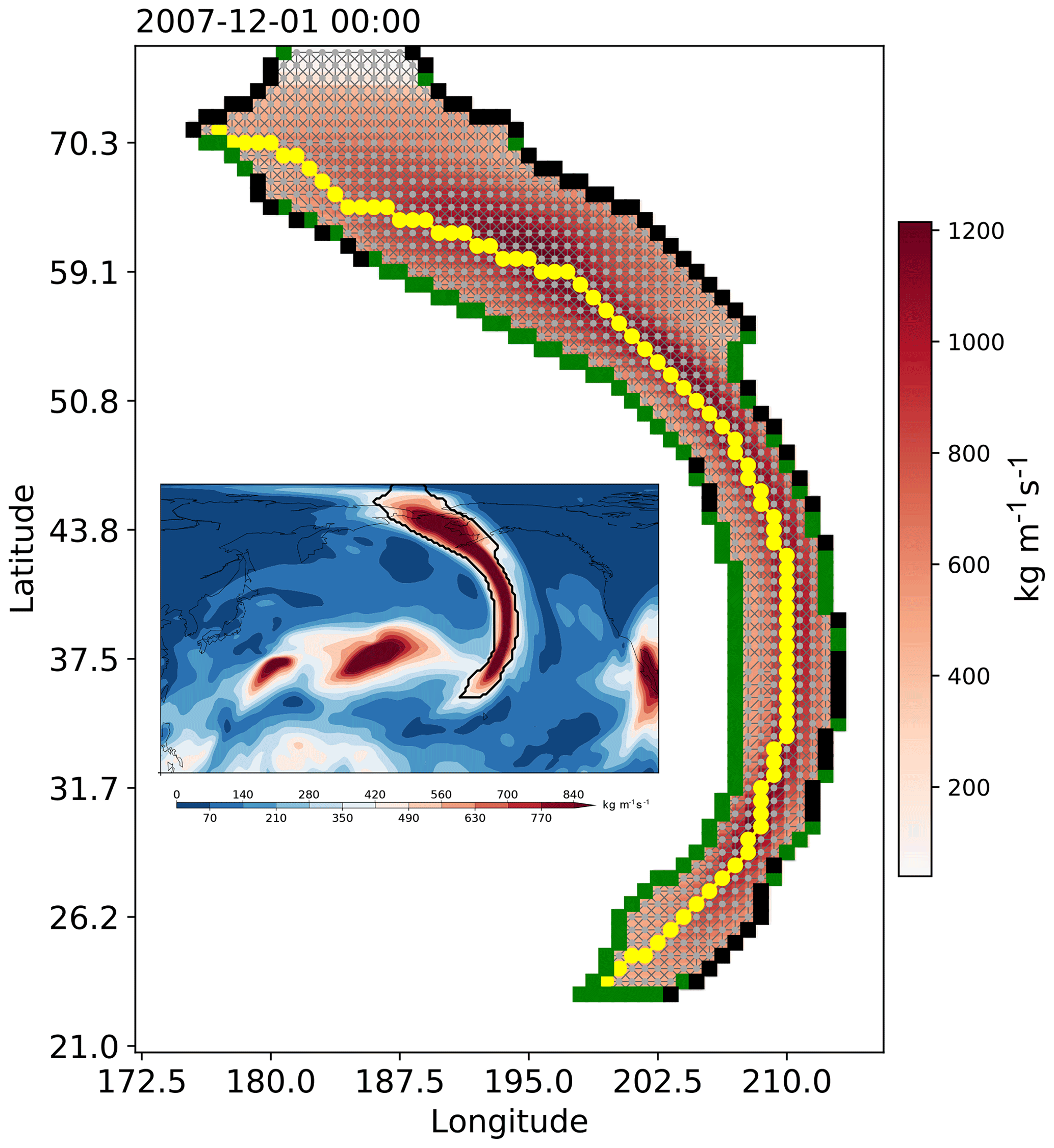
Figure 2Application of the axis-finding algorithm on the AR in the North Pacific on 1 December 2007 at 00:00 UTC. IVT within the AR is shown as colors, in kg m−1 s−1. The region of the AR (Ik) is shown as a collection of grey dots, which constitute nodes of the directed graph. Edges among neighboring nodes are created. A square marker is drawn at each boundary node and is filled with green if the boundary node has net input moisture fluxes () and with black if it has net output moisture fluxes (). The found axis is highlighted in yellow. The inset image shows the IVT distribution over the North Pacific with the selected AR highlighted in black contour.
2.4 Tracking ARs across time steps
For each AR, we take seven (roughly) evenly spaced points along the AR axis as “anchors” that collectively describe the approximate location of the AR. To measure the inter-AR distances, we borrow the Hausdorff distance that is commonly used in compute vision to measure the geometrical similarity between 2-D or 3-D objects (e.g., Huttenlocher et al., 1993; Vergeest et al., 2003) and modify it as follows.
Denote the anchor points of an AR at time t as and those of an AR at time t+1 as . The forward Hausdorff distance is defined as
namely, the largest great circle distance (dg) of all distances from a point in A to the closest point in B. And the backward Hausdorff distance is
Note that in general hf≠hb. Unlike the standard definition of Hausdorff distance that takes the maximum of hf and hb, we take the minimum of the two:
The rationale behind this modification is that merging/splitting of ARs mostly happens in an end-to-end manner, during which a sudden increase/decrease in the length of the AR induces misalignment among the anchor points. Specifically, merging (splitting) tends to induce large backward (forward) Hausdorff distance. Therefore, offers a more faithful description of the spatial closeness of ARs. For merging/splitting events in a side-to-side manner, this definition works just as well.
This formulation effectively summarizes inter-AR closeness into a single distance measure; therefore, tracking of ARs across time steps can be achieved using similar techniques as in the tracking of tropical cyclones or storms.
There are two possible manners in which such feature tracking can performed: (i) in a “simple path scheme” where the track of a feature across time forms a topological simple path, i.e., no merging nor splitting is allowed, and a system can only appear at one location at any given time; and (ii) in a “network scheme” where features are allowed to merge/split for arbitrary number of times, and their combined tracks form a directed network. The former scheme is simple to implement and suitable for occurrence statistics, as each occurrence is counted only once. In the later scheme, an occurrence may be included in more than one track if it is involved in a merging or splitting. Therefore, the latter scheme is more suitable for case studies where the full lifetime of a system or interactions between systems are of interest.
In this study, we focus on the simple path-tracking scheme. To achieve that, a nearest neighbor method is used that the two AR axes found in consecutive time steps with a Hausdorff distance ≤1200 km are linked, with an exclusive preference for the smallest Hausdorff distance. The full algorithm is given in Sect. A3 in the Appendix. Two selected cases using the network tracking scheme are given as an illustration.
3.1 Sensitivity of AR occurrence numbers to parameters
With the geometric metrics kept constant, the parameters that affect the detection performance of the THR algorithm are the temporal (t) and spatial (s) sizes of the structuring element. ARs found with a given parameter combination are labeled as “THR-tx-sy”, where x (y) denotes the value of t (s), in units of days (number of grid cells).
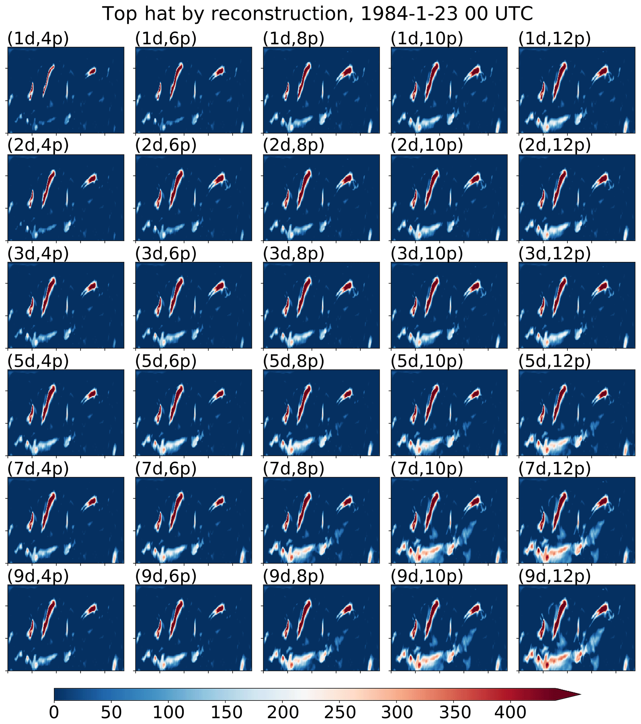
Figure 3IVT anomalies (in kg m−1 s−1) from the THR process on 23 January 1984 at 00:00 UTC. Subplots are results obtained using different combinations of the time (t) and space (s) parameters of the 3-D structuring element in the THR process, and the subplots are labeled in a format of (td, sp), with d being short for “days” and p for “pixels”. From row 1 to row 6, t increases from t=1 to t=9 d. From column 1 to column 5, s increases from s=4 pixels to s=12 pixels, with a step of 2. Axes' information has been omitted for brevity, and the domain is the same as in Fig. 1a.
Shown in Fig. 3 are the IVT anomalies from the THR process on 23 January 1984 at 00:00 UTC, obtained using 30 different combinations of t and s. The IVT data are computed as IVT , where u and v are the vertically integrated horizontal moisture flux components, with a 0.75∘ horizontal resolution and a 6-hourly temporal resolution. u and v data are obtained from ECMWF's ERA-I reanalysis product (Dee et al., 2011). It has been demonstrated that the choice of reanalysis dataset contributes little to the resultant detection statistics (Ralph et al., 2018; Shields et al., 2018). It can be seen that the filtering process is rather insensitive to the size/shape of the structuring element. All three major ARs and the moderate one at the center of the map are isolated in each combination, and notable differences only appear in the tropical reservoir and around the edges of the isolated ARs. In particular, a larger structuring element retains more tropical signals and gives larger AR regions. This is because the spatiotemporal size of an enlarged structuring element starts to deviate away from the transient nature of ARs and would tend to include larger systems.
As a comparison, we also applied two conventional detection methods on the same ERA-I data. For the constant IVT anomaly threshold approach, IVT anomalies are first obtained by subtracting from the 6-hourly IVT data a low-frequency component, which is the mean annual cycle (during January 2004 to December 2010) smoothed by a 3-month moving average. The use of anomalous IVT instead of absolute values helps remove slow-varying features and makes a fixed threshold more applicable across basins, seasons and years (Mundhenk et al., 2016). The only parameter used in this method is the cut-off IVT value; therefore, ARs found by an IVT anomaly threshold of, for instance, 250 kg m−1 s−1, are labeled as “IVT250ano”.
To detect ARs using a percentile-based threshold, we first computed the 85th IVT percentile for each of the 12 months within all 6-hourly time steps during the 3-month period centered on that month, within a 9-year moving time window. For instance, the months of June–July–August (JJA) during 1996–2004 are used to find the 85th percentiles for the month of July 2000. Then the threshold used to detect AR candidates is the 85th IVT percentile, or a fixed 100 kg m−1 s−1, whichever is larger, as in Guan and Waliser (2015). ARs found by this method are labeled as “IVT85%”.
As the parameters of THR and constant-IVT methods are of different natures (spatiotemporal scales versus horizontal vapor flux), it is not obvious how to design directly comparable perturbation ranges. Therefore, the perturbation range of constant IVT threshold is arbitrarily chosen to be 200–300 kg m−1 s−1 – a 20 % perturbation around the standard 250 kg m−1 s−1 value. The perturbation of the t parameter is set to 1–8 d, and s to 3–10 grids, about 50 %–75 % perturbation around the standard values of t=4 d and s=6 grids. The percentile value serves the same role in affecting detection results as the constant IVT threshold; therefore, only the 85th percentile result is presented as a reference.
The same set of geometric filtering is applied to results from the THR, constant IVT thresholding and the IVT85% methods. The minimal length requirement is set to 2000 km. It is important to keep in mind that much of the sensitivity in the number of detected ARs comes from the interplay between initial detection and subsequent geometric filtering (Ralph et al., 2018).
Figure 4 shows the mean annual number of AR occurrences over the North Pacific during 2004–2010 from different methods. The numbers are the AR occurrences within all 6-hourly time steps, evenly divided into calendar years. It could be seen that the annual mean detection number displays lower sensitivity to the THR t parameter at fixed s (Fig. 4a) and similarly to the s parameter at fixed t (Fig. 4b), compared with the sensitivity to IVT thresholds (Fig. 4d). Detection number varies more when both t and s change simultaneously, as shown in Fig. 4c, from 2208 at the smallest (t=1 d, s=3 grids) scale to 2730 at the (t=6 d, s=8 grids) scale. The tendency of increasing AR numbers with enlarging scales is due to the interplay between initial detection and geometric screening. However, as long as the parameters are set around the typical synoptic spatiotemporal scales, the resultant AR occurrence numbers are more or less the same.
In comparison, the constant IVT threshold method produces fewer ARs as one raises the threshold, creating a drop of 848 from the IVT200ano to the IVT300ano setup. The effect from varying IVT thresholds is intuitive: as one raises the threshold, smaller regions are retained. When coupled with a minimal size requirement, more get filtered out.
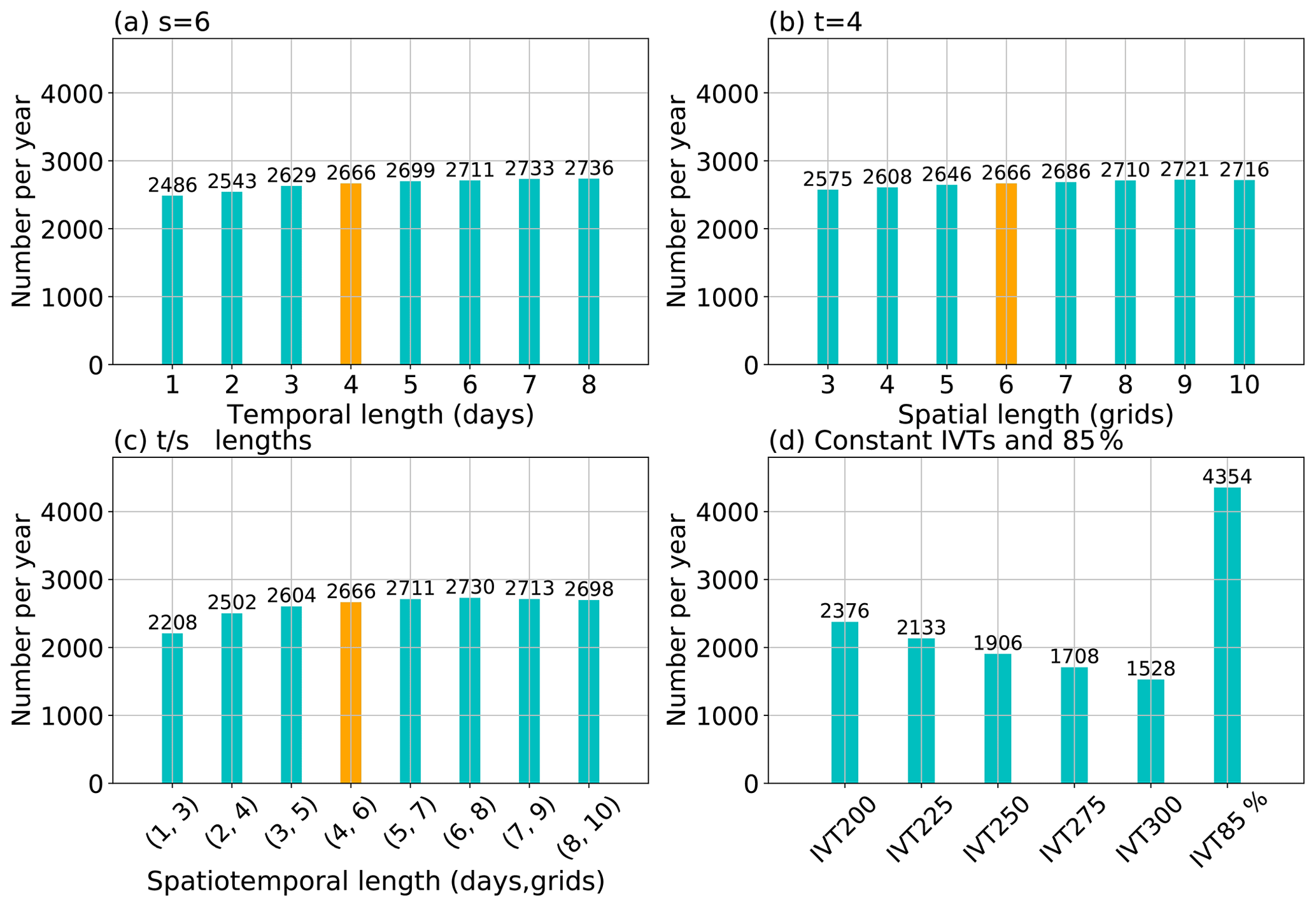
Figure 4Average annual number of AR occurrences over the North Pacific during 2004–2010. (a) AR occurrence numbers by the THR method with various time (t) parameters and a fixed space parameter (s=6). (b) Similar to panel (a) but for fixed time (t=4) and varying space (s) parameters. (c) Results from the THR method with time (t) and space (s) varying simultaneously from the lower bound of t=1 d, s=3 grids to the upper bound of t=8 d, s=10 grids. (d) AR occurrences from the constant IVT thresholding method with the threshold value ranging from 200 to 300 kg m−1 s−1 and the result from the IVT85% method as in the last column.
Also note that the IVT85% method reports more than double the number of ARs of the highest THR method (Fig. 4d). As will be shown in later sections, this method tends to produce ARs with notably different features compared to the other two and is likely because the geometric metrics listed in Sect. 2.2 are insufficient in effectively filtering some weak plumes. Specifically, it is likely that the requirement of a minimal mean poleward IVT component and mean IVT direction being within 45∘ of the AR shape orientation that are applied by Guan and Waliser (2015) but absent in this study is making the greatest difference.
Results in Fig. 4 suggest that the THR-t4-s6 method reports 760 more AR occurrences per year than the IVT250ano method. By applying a matching method based on areal overlap ratio, we are able to look closer at the degree of agreement between these two methods in terms of AR occurrences and their accounted IVTs. Besides occurrence numbers, there are also some differences in the geographical locations of the detected ARs by different methods, with different implications in the seasonally accumulated meridional moisture transport related to ARs. Details of this are beyond the scope of this study and are discussed further in Xu et al. (2020b).
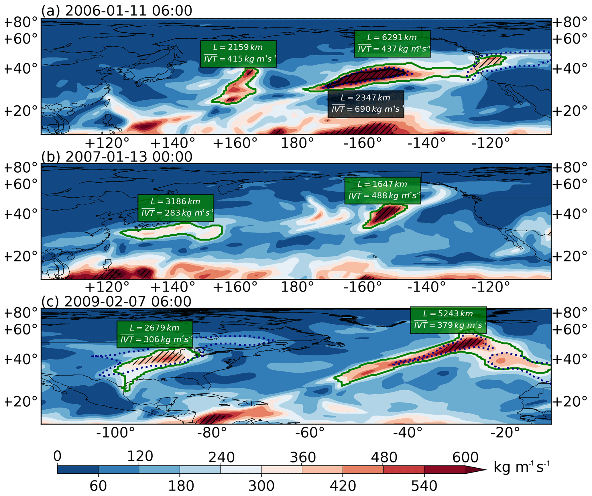
Figure 5Snapshots of IVT distributions on (a) 11 January 2006 at 06:00 UTC over the North Pacific, (b) 13 January 2007 at 00:00 UTC over the North Pacific and (c) 7 February 2009 at 06:00 UTC over the North Atlantic. ARs found by the THR-t4-s6 method are drawn in solid green contours, those by the IVT250ano method in solid black contours and those by IVT85% in dotted black contours. Length (in km) and area-averaged IVT (in kg m−1 s−1) for the THR-t4-s6 (IVT250ano) ARs are labeled out in green (black) boxes. Hatching indicates areas where the IVT anomalies are above the 250 kg m−1 s−1 threshold.
3.2 Comparison of selected cases
Figure 5 shows some selected cases where an AR occurrence is detected by the THR-t4-s6 method but not by IVT250ano. ARs found by the former are drawn in solid green contours and the latter in solid black contours. On 11 January 2006 at 06:00 UTC (Fig. 5a), both methods detect the stronger AR over the northeastern Pacific; however, the weaker one at ∼160∘ E is missed by IVT250ano. This is because the region where IVT anomalies are above the 250 kg m−1 s−1 threshold is too small, as indicated by the hatching. This AR is not detected by IVT250ano until 12 January 2006 at 12:00 UTC, at which time it has migrated to ∼180∘ E. Then, 4 d later (16 January 2006 at 12:00 UTC), it makes landfall onto the North American continent. Figure S1 in the Supplement shows the entire life cycle sequence of this AR.
Similarly, the northwestern Pacific AR on 13 January 2007 at 00:00 UTC is missed by the IVT250ano method (Fig. 5b). The THR method identifies this AR occurrence as one with a length of 3186 km and an average absolute IVT of 283 kg m−1 s−1. Then, 30 h later, IVT250ano detects this AR until 18 January 2007 at 06:00 UTC, at which time it is just about to make landfall in North America (Fig. S2). Meanwhile, THR traces this particular AR throughout this period until 1 d after it is last seen in the IVT250ano detection (Fig. S2). Also shown in Fig. 5b is another AR occurrence at ∼155∘ W that is solely detected by THR. This AR is not detected by IVT250ano until 15 January 2007 at 06:00 UTC (Fig. S2).
Figure 5c shows another case in the North Atlantic. The AR in question is propagating over the eastern North America at the time of 7 February 2009 at 06:00 UTC. The life cycle sequence in Fig. S3 indicates that this AR never appears in the IVT250ano detection until its dissipation on 13 February 2009 at 12:00 UTC just south of Iceland. Figure 5c also shows another AR occurrence over the northeastern Atlantic that is missed by the IVT250ano method but detected by THR.
It could be seen that the exclusive THR AR detection tends to correspond to the genesis or dissipating stages of some well-defined AR tracks (Fig. 5a, b) or in other cases the entire life cycle of some weak systems as in Fig. 5c. Ralph et al. (2018) also suggested that discrepancies among methods are smaller in cold seasons than in warm seasons, in more active years than in quieter years and during time steps with higher observed IVT than those with lower IVT. In summary, sensitivity to detection methods is much greater for weaker systems.
It was also observed that methods with more restrictive geometrical criteria tend to report less detection compared with those with comparable magnitude thresholds but are more permissive in the geometrical requirements (Ralph et al., 2018). In most of the existing detection methods, geometrical filtering is applied as an extra step after the initial region detection. However, these two steps are inherently closely coupled: once the candidate region is determined, so is its geometry, and with the help of a sensible length estimate, its length as well. Therefore, for a magnitude-thresholding detection method, the choice of the threshold to some extent already determines the expected geometrical extent of the passing candidates, with largely predictable behavior as one adjusts the threshold: raising the threshold level restricts the sizes of the detected ARs, and vice versa. However, what is less predictable is the resultant AR statistics when applying the same threshold to data across multiple decades when low-frequency drifts may be present or to climate projections where different model biases are to be expected.
The sensitivity and uncertainty embedded in geometrical constraints still exist in the THR method but to a much lesser extent. Weaker systems as shown in Fig. 5 are more likely to be detected together with the most intensive ones. It also implies that the geometrical filtering is more of an independent criterion rather than closely coupled with the initial region detection process. This allows for the inclusion of systems that are weaker (note that in climate scale, or with different model biases, it is less obvious how weak is weak) in intensity but sizable in geometry. As shown above and will be discussed later, this often leads to the captured AR tracks having a fuller life cycle. As the strength and size criteria are decoupled, the user can still apply a subsequent magnitude filtering on the maximum and/or average IVT to obtain the subset of a certain intensity level. Therefore, it offers greater control power without completely breaking the compatibility with existing methods.
As a reference, Fig. 5 also shows as dotted black contours the ARs detected by the IVT85% method. This method displays improved sensitivity to weaker IVT signals, as in the case of the landfalling AR in Fig. 5a and the one over the eastern North America in Fig. 5c. However, it still misses the three ARs in Fig. 5a and b. Also note that the THR ARs on the eastern side of the map in Fig. 5a and Fig. 5c enclose more than one local IVT maxima in their region contours. This can happen when merging or splitting creates two nearby transient plumes and can subsequently contribute to the geometry-related uncertainties. A method has been developed to separate such “multi-core systems” into “single-dome” ARs and will be introduced in a future update of the algorithm.
3.3 Sensitivity of AR shapes and IVT intensities to parameters
Some geometrical features and IVT intensities of the ARs identified by the three methods are summarized in Fig. 6. Considering the low sensitivity to either t or s parameters with the other one fixed in the THR method, only the parameter combinations when both t and s vary simultaneously are included.
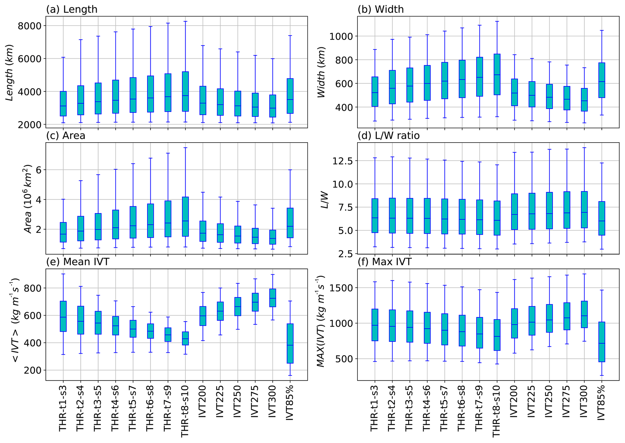
Figure 6Distributions of (a) AR length (in km), (b) width (in km), (c) area (in 106 km2), (d) length ∕ width ratio, (e) mean IVT averaged over AR region (in kg m−1 s−1) and (f) maximum IVT within the AR region (in kg m−1 s−1) of ARs identified by different methods, during the period of 2004–2010. Box ends denote the interquartile range of the distribution, with the median as the line in the middle. Box whiskers denote the 5th and 95th percentiles.
Figure 6 shows that enlarging the THR structuring element tends to produce ARs with larger sizes, and this can be seen in the length (Fig. 6a), width (Fig. 6b) and area (Fig. 6c) distributions. (Note that width is defined as the effective width, i.e., the ratio of area over length.) However, the length ∕ width ratio remains about constant (Fig. 6d). Raising the constant IVT threshold has the opposite effect, where the resultant ARs are progressively shorter (Fig. 6a), narrower (Fig. 6b) and smaller in size (Fig. 6c).
Figure 6e suggests that larger-sized ARs tend to have lower mean IVT values, and this is true among THR and constant IVT threshold methods. Although the maximum IVT follows a similar trend (Fig. 6f), the differences are much smaller. This is because when taking the average over the region of larger-sized ARs, the mean values get “diluted” more during the spatial averaging process, yet the maximum values are largely immune to this “dilution”. Therefore, the lower mean IVT values of THR ARs are primarily due to their larger sizes than due to the inclusion of weaker systems. The variation among constant IVT threshold methods is also consistent with Shields et al. (2018) in that higher threshold on IVT produces higher average IVT intensities.
Results of the IVT85% ARs are also displayed as a reference. ARs found by this method display comparable size distributions as that by THR-t2-s4 method (Fig. 6a–d) but with notably weaker mean (Fig. 6e) as well as maximum IVT distributions (Fig. 6f). Combined with the high number of ARs found by IVT85% as shown in Fig. 4d, it could be inferred that a good number of these are fairly weak systems that get ignored by the other two.
The sizes of ARs constitute an important source of uncertainty in many AR-related estimates (Ralph et al., 2018; Shields et al., 2018). For instance, Rutz et al. (2014) showed that by lowering the IVT threshold from 300 to 200 kg m−1 s−1, the resultant landfalling AR frequency onto the North American coast rises by ∼50 % (see their Fig. 5). A similar concern was also raised in Mundhenk et al. (2016) when quantifying North Pacific AR frequencies. Currently, no metrics have been developed to objectively quantify the appropriateness of the AR boundary definition. We offer some brief discussions on this topic from a segmentation cost perspective in Sect. A5 in the Appendix.
Besides the quantification of AR occurrences, prediction of ARs also requires tracking ARs across time steps. Figure 7a shows an example of the tracking algorithm applied on THR-t4-s6 ARs found on 2 December 2007 at 00:00 and 06:00 UTC, drawn with dashed blue and red lines, respectively. A blue (red) arrow indicates the forward (backward) Hausdorff distance between a pair of ARs that get linked. It could be seen that for pairs that are well separated or relatively clustered, the Hausdorff distance correctly measures the inter-AR closeness and enables the nearest neighbor algorithm to make the correct associations. Note that the minimal length requirement is relaxed to 800 km, but it is required that the same AR reaches ≥2000 km for at least one time step during its lifetime.
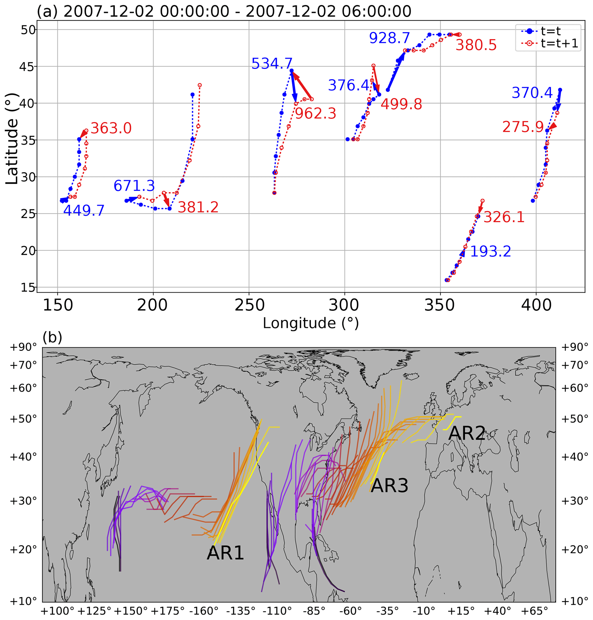
Figure 7(a) Tracking of ARs across 2 December 2007 at 00:00 and 06:00 UTC using the nearest neighbor algorithm. ARs on 2 December 2007 at 00:00 UTC are represented by their anchor points joint by dashed lines and are drawn in blue, and ARs on 2 December 2007 at 06:00 UTC are drawn in red. Blue (red) arrows indicate the forward (backward) Hausdorff distance among paired ARs, and the distances (in km) are labeled nearby. (b) Tracks of three selected ARs represented by their axes. The life cycle of an AR is represented as the black–yellow transition in the coloring. Other ARs during the same period are omitted for brevity.
Figure 7b shows the tracks of three selected ARs in November–December 2007 obtained using the simple path scheme. The axes of the ARs are drawn with a black–yellow color scheme, with the transition representing the stages of their life cycle. The two ARs originating from Pacific (AR1, AR2) have experienced the association process as shown in Fig. 7a. AR1 reaches a length of ∼4700 km shortly before its landfall onto the western coast of the North America on 4 December 2007 at 06:00 UTC. AR2 starts as an eastern Pacific system on 1 December 2007 at 00:00 UTC and survives the cross-continent and cross-basin travel before its European arrival on 7 December 2007 at 06:00 UTC, at which point the AR has shrunk to a fairly short 960 km. AR3 is initially fueled by a tropical cyclone in the Caribbean Sea and is joined by another plume (not shown in this figure) coming from the eastern Pacific during its eastward travel and dissipates halfway through its North Atlantic propagation.
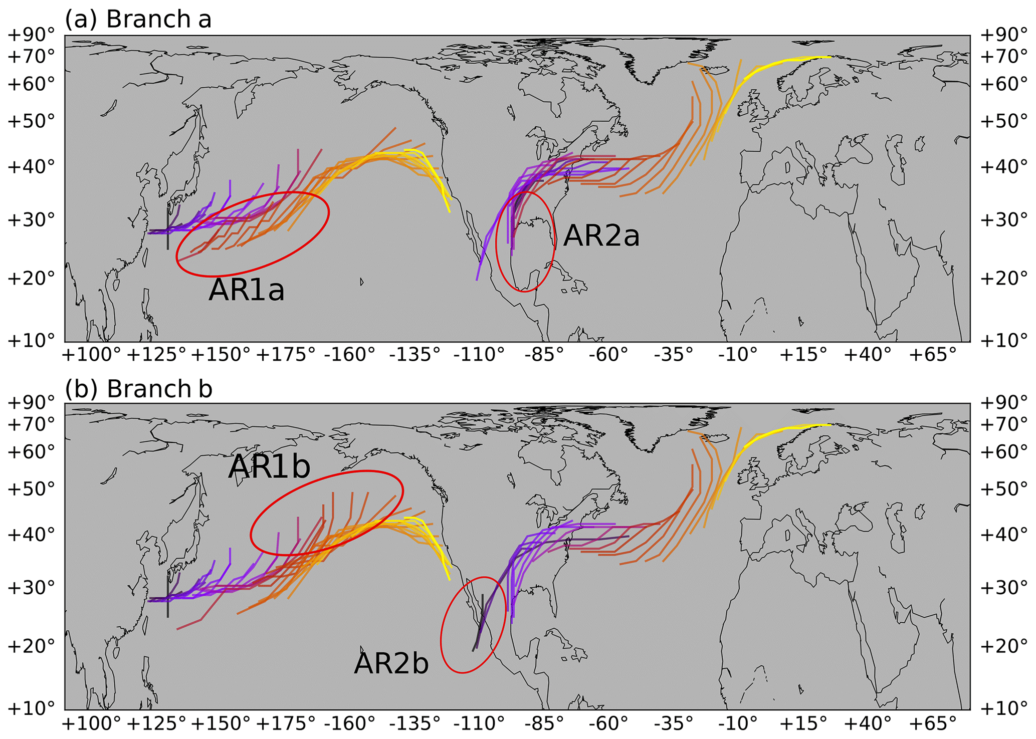
Figure 8Tracks of two ARs obtained using the network scheme. Each of the two ARs (AR1 and AR2) has two branches (branch a and branch b) in their tracks, shown in panels (a) and (b), respectively. The same color scheme as in Fig. 7 is used to represent their life cycles. The different branches of a single AR track are highlighted in red ellipses.
Figure 8 shows two selected AR tracks obtained using the network scheme, where merging and splitting are captured. To achieve this, three consecutive applications of the nearest neighbor algorithm are performed, with different input arguments each time. More details are given in Sect. A4 in the Appendix. The first selected case (AR-1) starts from the northwest Pacific on 21 December 2007 at 12:00 UTC and splits into a southern branch (AR-1a, shown in Fig. 8a) and a northern branch (AR-1b, Fig. 8b) during its eastward propagation. The two branches then merge into one shortly before the North American arrival on 29 December 2007 at 12:00 UTC. In fact, the life cycle of this AR is further complicated by the joining of a third branch originating from another tropical system. We have omitted the third branch for the sake of clarity. AR-2 demonstrates a merging case in which a system from the Gulf of Mexico (AR-2a; Fig. 8a) is joined by an eastern Pacific one (AR-2b; Fig. 8b), and the combined track then makes European landfall. It has been estimated that about 25 % of wintertime extratropical cyclone tracks experience at least one merging and/or splitting during their lifetime (Hanley and Caballero, 2012). The proposed method enables similar analysis on AR tracks and their possible links with merging or splitting cyclones.
The simple path scheme is then applied to all Northern Hemisphere ARs found by the THR-t4-s6 method during the November–April seasons of November 2004 to April 2010. Depending on the AR centroid at genesis time, those lying within 120∘ E–100∘ W are labeled “Pacific”, and those within 100∘ W–20∘ E are labeled “Atlantic”. After removing tracks lasting shorter than 24 h, it is found that, on average, both the North Pacific and North Atlantic have about 80 AR tracks during the November–April season. More notable difference is observed in track durations, as shown in Fig. 9. The median of the Pacific track durations is 78 h; that of the Atlantic is 66 h. Such a difference is largely attributed to those tracks lasting for 150 h or beyond and is consistent with the greater longitudinal span of the Pacific basin. Note that the duration is defined as the lifetime of individual AR tracks and is distinct from a per grid, Eulerian definition as in, for instance, Guan and Waliser (2015), Rutz et al. (2014, 2015) and Sellars et al. (2017), who measured the contiguous time spans when a grid cell experiences AR occurrences.
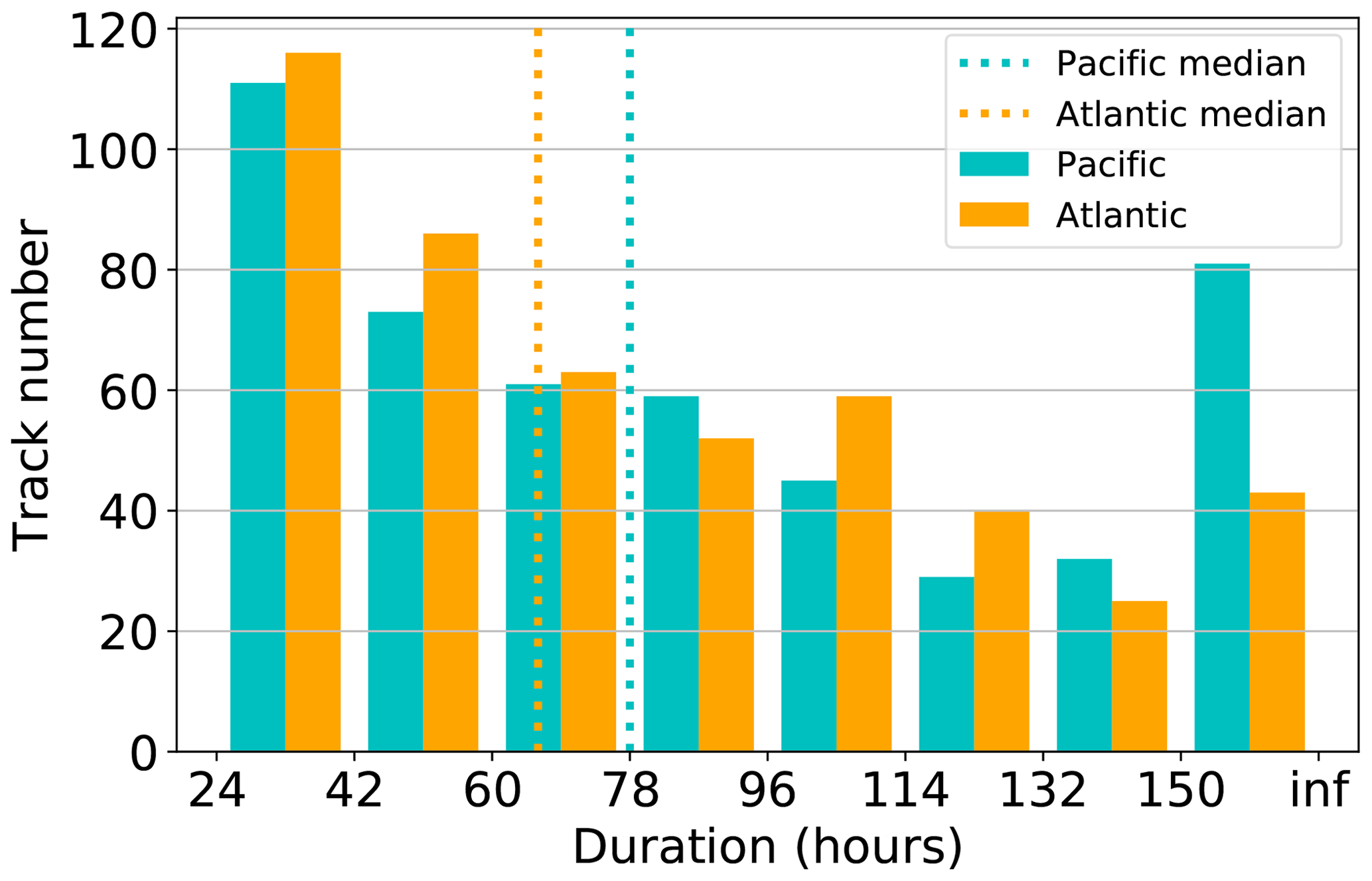
Figure 9Distribution of track durations (in hours) of AR tracks in the North Pacific (cyan) and North Atlantic (orange). The “inf” label is used to form the right bin edge for the last bin which includes all tracks lasting longer than 150 h.
Figure 10 displays the movements of all Northern Hemisphere AR tracks during the November–April seasons of November 2004 to April 2010. The geometrical centroid of the AR region is used as a proxy to location, and coloring represents the maximum IVT within the AR region at each time step. It could be seen that distributions of AR tracks overlap well with the storm track regions of the North Pacific and North Atlantic basins, with a southwest–northeast orientation (Hodges, 1994). ARs of both ocean basins can be traced back to the western boundary warm current regions – the Kuroshio Current for the Pacific and the Gulf Stream for Atlantic. For the Atlantic, a considerable number of ARs also originate from the Gulf of Mexico. Keep in mind that an arbitrary 23∘ N latitude requirement has been applied during the detection stage which to some extent prevents the genesis locations to be traced back to the main moisture reservoir within the tropics.

Figure 10Movement of Northern Hemisphere AR tracks as indicated by the geometrical centroids during the November–April seasons of November 2004 to April 2010. Color represents the maximum IVT within the AR region.
Note that Fig. 10 also shows an additional hot spot in the Middle East around the Red Sea, one across north Africa–Mediterranean–eastern Europe and another even weaker one over west Siberia. We would refrain from naming them ARs, as they conflict with the conventional AR definition in that they are weaker in strength, not ocean-originated and likely driven by different physical mechanisms. However, these are well organized (above 2000 km in length) and relatively persistent (can be tracked over 24 h) water plumes. The identification of such systems speaks to the greater adaptability of the THR method and its ability to encompass a wider range of transient water vapor plumes in a single framework.
To support our claim that the proposed THR method can be extended to IWV-based applications, we show only a selected case of IWV-based AR detection here because of the length limitation of the paper. Unlike IVT where the transition from tropical trades to extratropical westerlies creates a natural separation in the tropical and extratropical IVT distribution, ARs represented by IWV are usually well connected with the tropical reservoir. Therefore, some modification of the THR process is needed. The detailed procedure is given in Sect. A7 in the Appendix. A selected case is shown in Fig. 11.
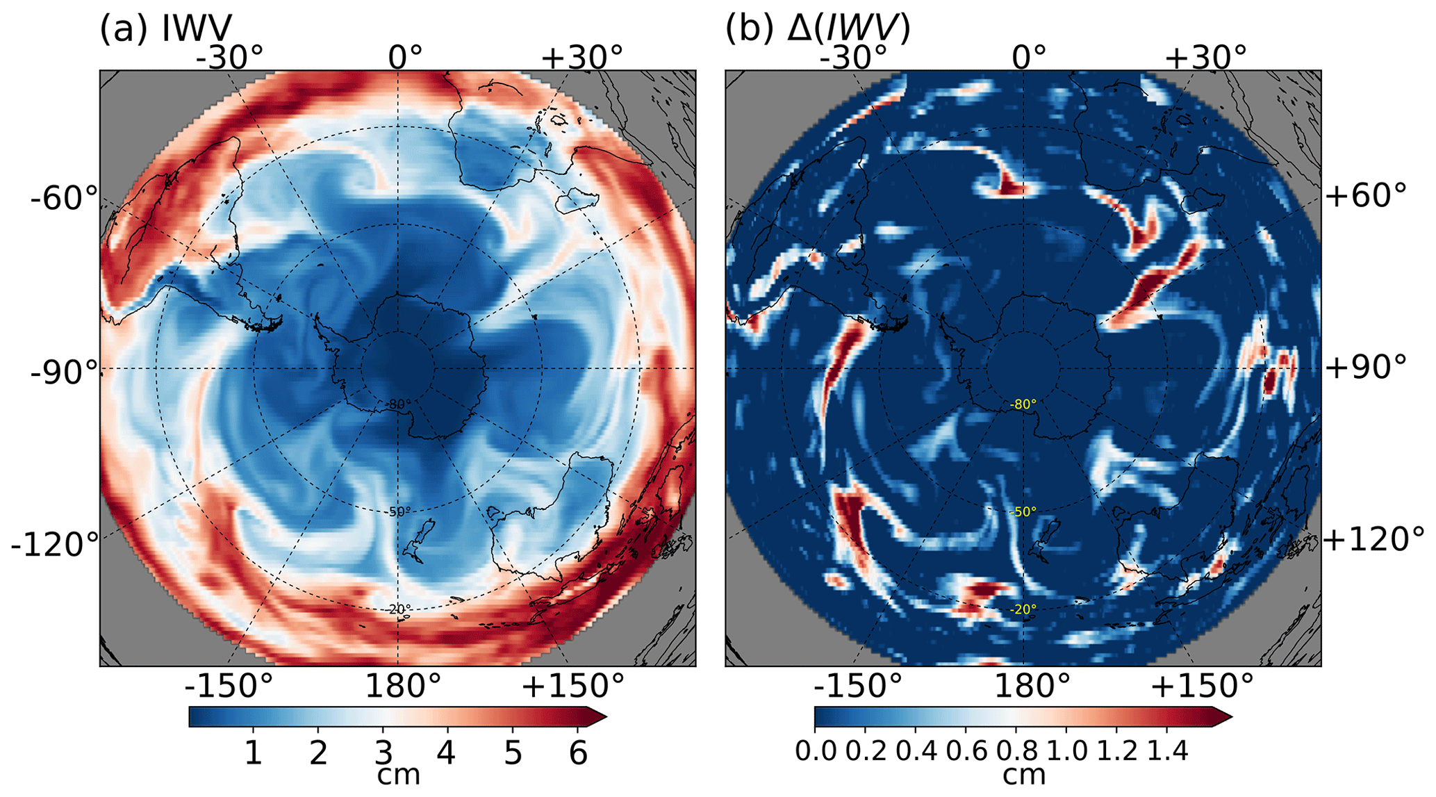
Figure 11(a) IWV in the Southern Hemisphere on 19 May 2009 at 00:00 UTC, in cm. (b) IWV anomalies in cm, obtained using a two-step THR, which uses a structuring element E with size t=4 d, s=6 pixels.
The IWV data from ERA-I are first projected onto the polar Lambert azimuthal projection before carrying out the two-step THR process, which uses the same structuring element of size t=4 d, s=6 pixels. Shown in Fig. 11a and b are the IWV and IWV anomalies, respectively, on 19 May 2009 at 00:00 UTC. The AR located at 60∘ E is moving towards Antarctica. This particular case has been documented by Gorodetskaya et al. (2014), in which the conventional 2 cm threshold value for IWV has been corrected by an empirical formula to cater to the decreased saturation capacity of the polar region. Note that although IVT is more than 2 orders of magnitude larger than the values of IWV, the THR method does not require a separate threshold for the IWV applications, and no polar adjustment is needed.
In this work, we propose a new set of automated AR detection and tracking methods. The THR algorithm exploits the transient nature of ARs to segment IVT signals. Compared with the intensities of AR-related vapor fluxes, the inherent spatiotemporal scale of AR is a more stable attribute. This makes the method less prone to the potential difficulties in reliably detecting ARs in a warming climate, and results from different models are more directly comparable when model biases may be present. It also demonstrates reduced sensitivity to parameter choices and greater tolerance towards a wider range of transient water vapor plumes and therefore has the potential of encompassing water plumes with various strengths into a unified framework. Furthermore, as strength is decoupled from the initial selection process, it is subject to the user to later select only those that meet a given strength standard, giving finer control power for different applications.
An intensity scale like those used to rank tropical cyclones has just been established for the landfalling ARs (Ralph et al., 2019). In the proposed scale, five intensity categories were devised, covering the lowest “weak” category, with observed IVT being 250–500 kg m−1 s−1, to the highest “exceptional” category, whose IVT level is 1250 kg m−1 s−1 or above, with extra duration factors taken into account in all categories. The difference in categories can mean the difference from a mild, beneficial atmospheric freshwater delivery to a hazardous extreme event that can cause damages measured in billions of dollars (Ralph et al., 2019). Therefore, it is advantageous for a detection method to have a wider detection spectrum rather than solely focusing on the most intensive events.
Besides the mostly commonly used magnitude-thresholding methods, new AR detection techniques are continually being developed. For instance, the ARTMIP project reported one machine-learning-based detection method that is also threshold-free (Shields et al., 2018). As the AR research matures, more inspirations from other disciplines like machine learning, image processing or computer vision are brought into the view of the AR community. Such inputs can offer some new perspectives of looking at various AR-related questions and can often lead to new discoveries that would have been obscured using conventional methods.
More physical information is encoded into the axis-finding method based on a directed graph model, creating an effective summary of an AR in the sense of geometry and physics. Problems of discontinuity, spurious branches, weak physical correspondence and difficulties in handling complex shapes are overcome in this method.
Lastly, tracking of ARs across time steps in a similar manner to the tracking of tropical cyclones and storms is achieved using a modified Hausdorff distance as the inter-AR proximity measure. Long-lived ARs spanning multiple days, having cross-continent or cross-basin tracks can be reliably traced through their tropical/subtropical origins to high-latitude landfall.
However, these methods come with their own limitations. Firstly, the THR method is considerably more complex than the constant thresholding method. Although it has been shown to have lower parameter sensitivity, sensitivities in other aspects still exist, particularly in the interplay between candidate region detection and the subsequent geometric filtering. Some ARs may fail the detection for their being just shy of a 2000 km length requirement or in other cases being too long because two nearby water plumes are merged together. Ambiguity in the shape of ARs still constitutes an important source of uncertainty in many AR-related statistics. A more accurate and controllable depiction of the AR shape is still in demand.
This appendix provides more technical details on AR detection using the THR algorithm, AR axis definition, inter-AR distance measure and tracking algorithms. A discussion on the AR sizes from a segmentation cost perspective is also given. Some select AR life cycle sequences are shown at the end.
A1 Top-hat reconstruction by dilation algorithm
Greyscale reconstruction by dilation can be defined as iterative applications of elementary geodesic dilations of a marker image M “under” a mask image I until convergence (Vincent, 1993). An elementary geodesic dilation is defined as
where M⊕B is the dilation of M by a flat structuring element B, and ∧ is the pointwise minimum operator. Intuitively, geodesic dilation spreads a local high-intensity value in the marker image M to its neighbors so long as it does not exceed values in the “mask” image I. The spread starts from the given “marker” and stops until no change can be made:
where is the reconstruction by dilation.
The “marker” image used is the greyscale erosion of the image I by a structuring element E:
The erosion and reconstruction by dilation computations are performed using the scikit-image software package (van der Walt et al., 2014) designed for imaging processing in the Python programming language.
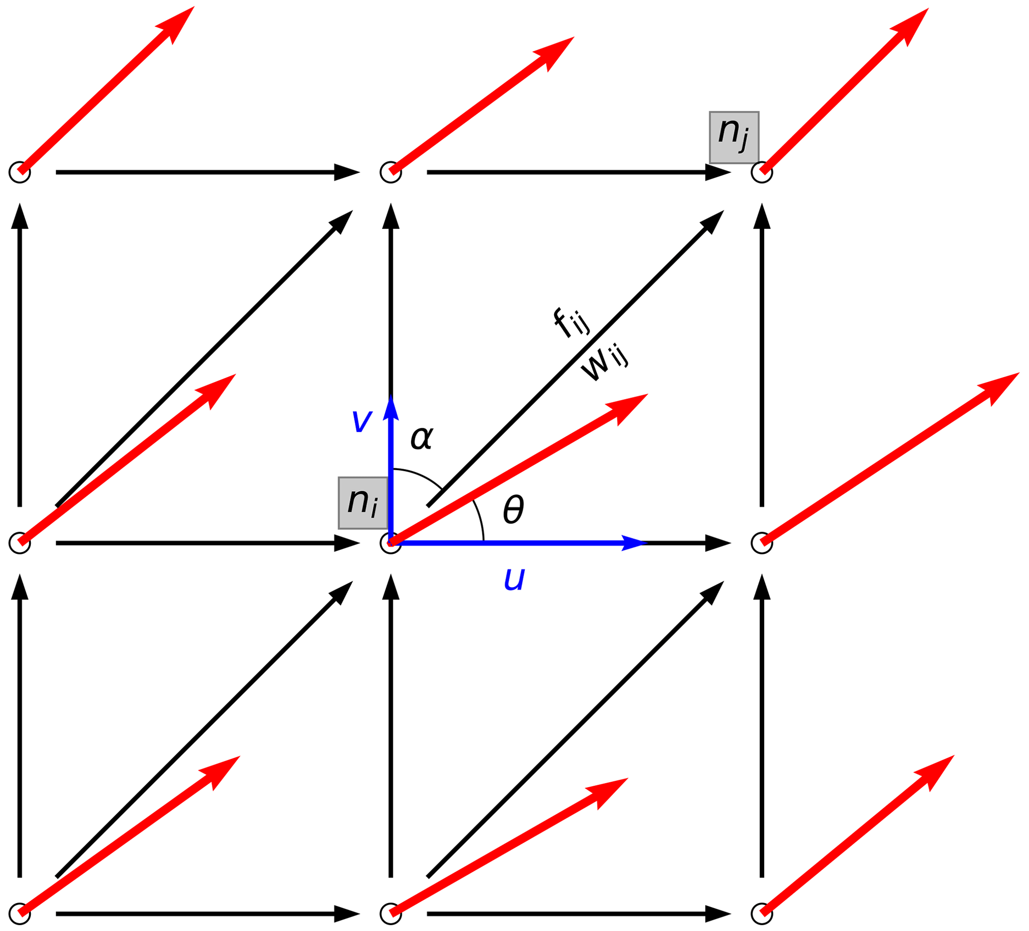
Figure A1Schematic diagram illustrating the planar graph built from the AR pixels and horizontal moisture fluxes. Nodes are taken from pixels within region Ik and are represented as circles. Red vectors denote IVT vectors. The one at node ni forms an angle θ with the x axis and has components (u, v). Black arrows denote directed edges between nodes, using an 8-connectivity neighborhood scheme. The edge between node ni and nj is eij and forms an azimuth angle α with the y axis. wij is the weight attribute assigned to edge eij, and fij is the along-edge moisture flux.
A2 Define the directed planar graph for axis finding
A directed planar graph is built from Ik, which is the binary mask defining the AR region, using the coordinate pairs (λk,ϕk) as nodes (see Fig. A1 for an illustration). At each node, directed edges to its eight neighbors are created, so long as the moisture flux component along the direction of the edge exceeds a user-defined fraction (ϵ) to the total flux. The along-edge flux is defined as
where fij is the flux along the edge eij that points from node ni to node nj, and α is the azimuth angle of eij.
Therefore, an edge can be created if . Here, a relatively small ϵ=0.4 is used, as the orientation of an AR can deviate considerably from its moisture fluxes, and denser edges in the graph allow the axis to capture the full extent of the AR.
A3 Tracking ARs using the simple path scheme
To make an association between two ARs at consecutive time steps, a “nearest neighbor” approach is used. Formally, suppose n tracks have been found at t=t: , and has m new records: . The Hausdorff distances between all pairs of possible associations form a distance matrix:
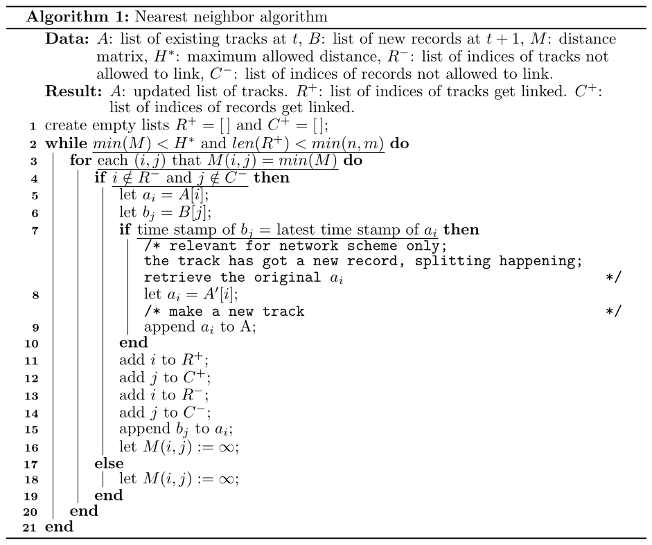
Then Algorithm A2 is called with these arguments: km, ). The algorithm iteratively links two AR records with the smallest distance, so long as the distance does not exceed a given threshold H*. It ensures that no existing track connects to more than one new record, and no new record connects to more than one existing track. After this, any left-over records in B form a new track on their own. Then the same procedure repeats with updated time . Tracks that do not get any new record can be removed from the stack list, which only maintains a few active tracks at any given time. Therefore, the complexity does not scale with time.
A4 Tracking ARs using the network scheme
Merging and splitting are allowed in this scheme, and the process consists of three consecutive applications of the nearest neighbor algorithm described above. Specifically, the process works as follows:
-
Make a copy A′ of the existing tracks A at time t=t, and a copy M′ of the distance matrix M.
-
Apply the nearest neighbor algorithm as in Algorithm A2:
where () contains the indices of tracks (records) that are linked in this process.
-
Merging is handled by repeating the nearest neighbor process as follows:
Note that the backed-up distance matrix M′ is used as it contains no infinities, and the argument masks out tracks that have been linked in the previous step, giving other tracks a chance to merge to the same new record.
-
Splitting is handled by repeating the nearest neighbor process as follows:
This time, new records that have been allocated in the previous steps are masked, giving other records a chance to split an existing track. Note that when splitting, the new record is appended to a back-up copy of the track from A′, and a new track is added to A after the split, as described in lines 7–9 of Algorithm A2.
-
Any left-over records in B form a new track on their own. Then, return back to step 1 with updated time .
It should be noted that this is not equivalent to a “link-all-neighbors” strategy, which will deny the preference to the nearest neighbor and create redundant links before (after) a merge (split). After a merge, merging tracks will have identical tracks thereafter; and for every split, a new track is created with its history retained. Therefore, there would be many duplicated records in this scheme.
A5 Segmentation cost estimates
The AR detection task can be viewed as a segmentation problem in the image-processing framework that a segment of the image (AR) is identified as the foreground image and thus getting separated from its background (the IVT distribution). In this formulation, a cost function can be defined to quantify the total intra-segment variances, as an evaluation of the effectiveness of the AR detection method in isolating high AR-related IVT values from its background:
where Nf, Nb are the number of grids in the foreground and background segments, respectively. If,i (Ib,i) denotes the pixel value of the foreground (background) image at location i, and the average across the segment is denoted (). The summations in square brackets quantify the total intra-segment variances. This is the same definition as used by Otsu (1979) in determining the optimal segmentation threshold. Either too small or too large an AR boundary definition would raise the cost function and result in a less effective separation of high-intensity values from the background. This is also equivalent to the cost function used in the k-means clustering algorithm (e.g., Dreyfus, 2005, chap. 7); in this case, the number of clusters is k=2, where the minimization of the cost converges to the solution. The normalization by maximum IVT (IVTmax) and the total image domain size (Nf+Nb) enables intercomparisons among different ARs. The total image domain is chosen as the bounding box of the AR boundary expanded out in four directions by five grid cells.
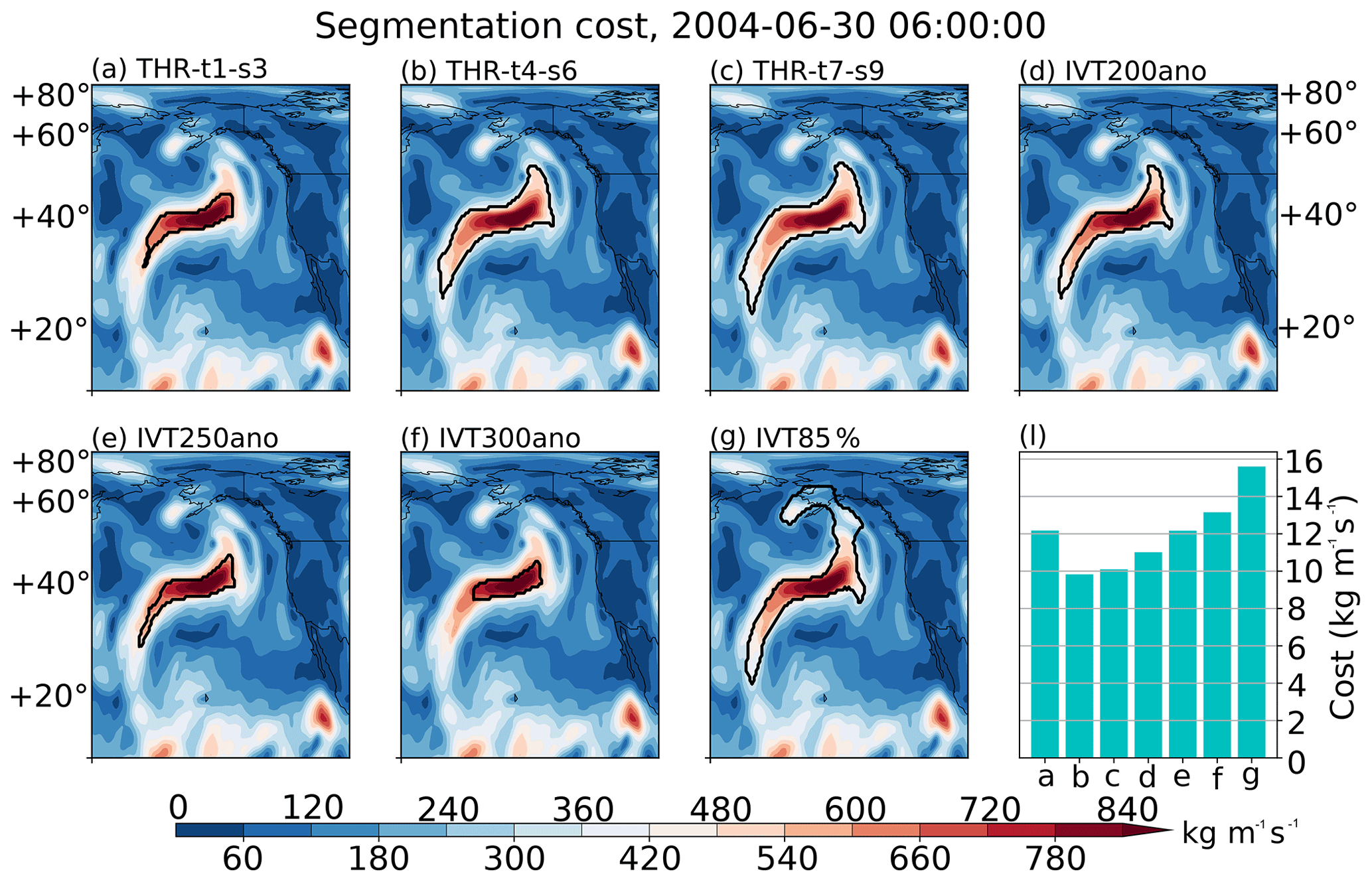
Figure A3IVT distribution on 30 June 2004 at 06:00 UTC over the northeastern Pacific (in kg m−1 s−1). Boundaries of ARs detected by (a) THR-t1-s3, (b) THR-t4-s6, (c) THR-t7-s9, (d) IVT200ano, (e) IVT250ano, (f) IVT300ano and (g) IVT85% methods are drawn with black curves. (i) The segmentation costs in all seven methods, in kg m−1 s−1.
Figure A3 compares the segmentation costs of an AR mutually detected by three THR methods, three constant IVT threshold methods and the IVT85% method, on 30 June 2004 at 06:00 UTC over the northeastern Pacific. Consistent with discussions in the main text, shrinking the THR structuring element has a similar effect to raising the constant IVT threshold that a smaller proportion of the transient IVT anomalies is segmented from the background. This particular time step is chosen because the segmentation cost comparison as shown in Fig. A3i is qualitatively consistent with the long-term 2004–2010 average (not shown). Although not specifically designed to minimize the segmentation cost, the THR-t4-s6 method that reflects the typical spatiotemporal scale of ARs gives the lowest cost.
A6 Explanations for the choices of the geometrical filtering criteria
The geometrical filtering criteria, including the maximum length/area, the minimum length, the maximum isoperimetric quotient, the minimum centroid latitude and the maximum Hausdorff distance in the nearest neighbor linkage process, are all determined from the physical natures of ARs as well as trial-and-error processes. The proposed method is mostly concerned with relaxing the hard and sensitive IVT strength threshold; therefore, the geometrical considerations are largely treated as controlled variables. Some further details regarding the choices of these criteria are given here.
A6.1 Maximum length/area
The maximum area/length requirements are set to fairly large values. The maximum length is set to 11 000 km, which is longer than the great circle distance (across the Pacific, ∼10 400 km) from Hong Kong (∼22.3∘ N, 114.2∘ E) to Seattle (∼47.6∘ N, −122.3∘ W). Assuming an average width of 700 km (which is on the larger side for typical ARs), this multiplies to an area of km2, which is smaller than the maximum area requirement set here (10×106 km2). These requirements are far larger than what could be expected from real-world AR sizes; therefore, they would only filter out erroneous detection.
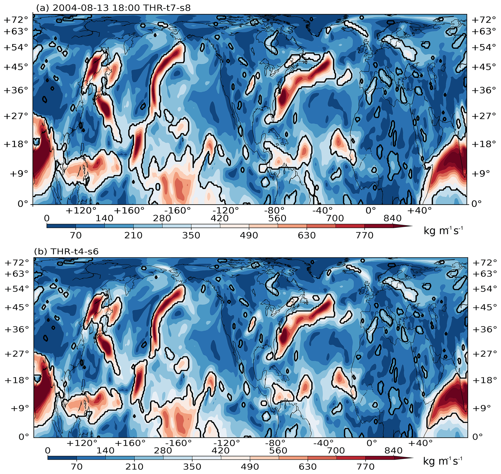
Figure A4Northern Hemisphere IVT distribution on 13 August 2004 at 18:00 UTC. Black contours denote connected regions where the THR anomalies are greater than zero. Panel (a) shows the result using THR-t7-s8 parameters; (b) shows the THR-t4-s6 parameters.
Regions with such large sizes only happen when two or more ARs are grouped together in one contour, or some of the ARs are connected with the large and continuous moisture plumes in the tropics to form a large continuous region. This happens more frequently when the structuring element E is set too large, as explained in Sect. 3.1. Figure A4 gives one such example. In Fig. A4a, the structuring element is set to t7-s8. This merges the Pacific ARs with tropical plumes to form a big connected region that later gets filtered out. Figure A4b is using the recommended t4-s6 parameters; this time the midlatitude signals are better separated from tropical ones so the Pacific AR is correctly retained. Those small noisy contours will be filtered by the minimum area requirement.
A method is being developed to separate ARs that have been mistakenly grouped together; once the new algorithm is fully ready, such maximum length/area criteria are no longer needed.
A6.2 Minimum length and maximum isoperimetric quotient
Some results regarding the sensitivities of AR numbers to the minimum length and maximum isoperimetric quotient criteria are given in Fig. A5.
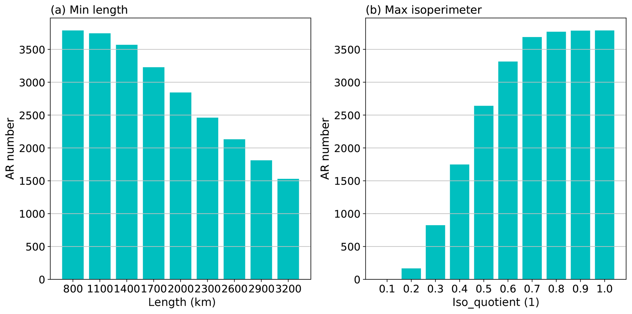
Figure A5(a) Average seasonal (November–April) AR numbers in the Northern Hemisphere during November 2004 to April 2010 when different minimum length criteria are applied. (b) Average seasonal AR numbers in the same time period when different maximum isoperimetric quotient criteria are applied.
For minimum length (Fig. A5a), sensitivity around the 800–1400 km range is fairly small. Also keep in mind that the 800 km threshold is used as a relaxed criterion to form a hysteresis thresholding couple with the standard 2000 km criterion, so it does not work quite the same as a single length threshold like in many other studies. This is an attempt to introduce some fuzziness into the geometric criteria, and it allows for a weaker feature (above 800 km in length) to be retained if and only if it is associated with a strong feature (longer than 2000 km).
For maximum isoperimetric, sensitivity around the 0.7 threshold used in this study is also fairly low (Fig. A5b).
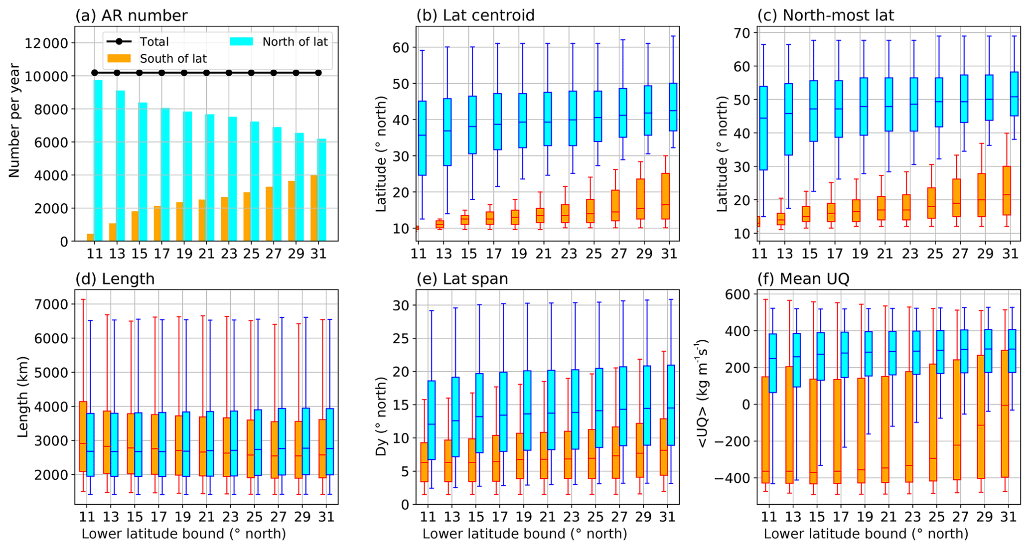
Figure A6Sensitivity tests on the lower latitudinal bound set to an AR's centroid. (a) Average annual AR numbers in the Northern Hemisphere during 2004 to 2008 when different lower latitude bounds are applied. Cyan (orange) bars show the number of ARs whose centroids are north (south) of the given lower latitude bound. The dotted black line is the sum of the two. (b) Distribution of the AR latitudinal centroids for ARs north (in blue) or south (in orange) of the given lower latitude bound. (c) Similar to panel (b) but for the distribution of the north-most axis point in ARs. (d) Similar to panel (b) but for the AR lengths. (e) Similar to panel (b) but for the latitudinal span of the ARs. (f) Similar to panel (b) but for the average zonal component of vertically integrated moisture flux (, in kg m−1 s−1).
A6.3 Minimum centroid latitude
Figure A6 gives some sensitivity tests regarding the choice of the lower latitudinal bound imposed on AR region's centroid. After detecting all ARs north of 10∘ N during 2004–2008, they are separated into two groups depending on their centroid being north or south of a given lower latitudinal bound. Values of this bound range from 11 to 31∘ N with an increment of 2∘. Detection north of this bound is represented in blue color in Fig. A6; detection south of this bound (but north of 10∘ N) is colored in orange.
It can be seen that ∼19–23∘ N is the range where the detection number shows reduced sensitivity to the latitudinal bound (Fig. A6a). The same is also true for the centroid latitude (Fig. A6b) and the latitude of the north-most axis point (Fig. A6c). This low-latitude detection has comparable or even larger lengths than the midlatitude ones (Fig. A6d) but with notably smaller latitudinal span (Fig. A6e). Furthermore, such low-latitude detection has primarily westward moisture fluxes, in contrast to the midlatitude counterparts (Fig. A6f). Therefore, they are mostly zonally oriented, large continuous vapor plumes carried by the tropical trades and incompatible with the midlatitude, storm-related AR definition taken in this study. This is also the primary reason for imposing a lower latitudinal bound.
A6.4 Maximum Hausdorff distance
The choice of 1200 km as the maximum Hausdorff distance during the track stage is based on references to similar maximum distance requirements used in extratropical cyclone tracking practices (Neu et al., 2013) and trial-and-error processes. Choices of 600, 800 and 1000 km (for 6-hourly intervals) are included in the Supplement Table A of Neu et al. (2013). We chose the largest one and gave it an extra margin to make it 1200 km, because in addition to movement, length variations also contribute to Hausdorff distance. The choice of this length has very low sensitivity and can be easily adjusted for data with different temporal resolution (e.g., scaled to 600 km for 3-hourly data or 2400 km for 12-hourly data).
A7 Two-step THR for IWV polar application
The 3-D erosion process is the same as for IVT, but instead of performing the reconstruction in three dimensions simultaneously, reconstruction on IWV is split into two consecutive steps. The first one uses a structuring element B that has only non-zero values along the time dimension. This constrains the geodesic dilation to the time dimension. Formally, this step involves
The second step takes Δ(IWV)t as input and performs a THR process in which geodesic dilation only expands in x and y dimensions.
Recall that the THR algorithm achieves segmentation according to the spatiotemporal “spikiness” of the data. As ARs in IWV are only spatially connected to the tropical reservoir which is temporally much more persistent, they can be separated in the time dimension THR. Then the second THR is concerned with spatial dimensions and helps retain spatially transient features. As an alternative to the two-step THR approach, a temporal filtering can be used to suppress the tropical signals. Then a similar 3-D THR process can be applied on the high-pass component of IWV.
The ERA-I reanalysis data used in the paper are publicly available. The implementations of the algorithms used in this work in the Python programming language are posted in the Zenodo repository (https://doi.org/10.5281/zenodo.3864592; Xu et al., 2020a).
The supplement related to this article is available online at: https://doi.org/10.5194/gmd-13-4639-2020-supplement.
GX and XM contributed to the development of the algorithms and data analyses. GX contributed to the writing of the manuscript, and all authors made significant contributions to its multiple revisions.
The authors declare that they have no conflict of interest.
This is a collaborative project between the Ocean University of China (OUC), Texas A&M University (TAMU) and the National Center for Atmospheric Research (NCAR) and completed through the International Laboratory for High Resolution Earth System Prediction (iHESP) – a collaboration by the Qingdao National Laboratory for Marine Science and Technology Development Center, Texas A&M University and the National Center for Atmospheric Research. The authors also give thanks to Chris Patricola from the Lawrence Berkeley National Laboratory, and Christine A. Shields from National Center for Atmospheric Research for their comments and suggestions for the manuscript.
This research has been supported by the National Key Research and Development Program of China (grant nos. 2017YFC1404000, 2017YFC1404100 and 2017YFC1404101) and the National Science Foundation of China (NSFC) (grant nos. 41490644, 41490640 and 41776013).
This paper was edited by Paul Ullrich and reviewed by two anonymous referees.
Camargo, S. J. and Zebiak, S. E.: Improving the detection and tracking of tropical cyclones in atmospheric general circulation models, Weather Forecast., 17, 1152–1162, https://doi.org/10.1175/1520-0434(2002)017<1152:ITDATO>2.0.CO;2, 2002. a
Dee, D. P., Uppala, S. M., Simmons, A. J., Berrisford, P., Poli, P., Kobayashi, S., Andrae, U., Balmaseda, M. A., Balsamo, G., Bauer, P., Bechtold, P., Beljaars, A. C. M., van de Berg, L., Bidlot, J., Bormann, N., Delsol, C., Dragani, R., Fuentes, M., Geer, A. J., Haimberger, L., Healy, S. B., Hersbach, H., Hólm, E. V., Isaksen, L., KÅllberg, P. W., Köhler, M., Matricardi, M., McNally, A. P., Monge-Sanz, B. M., Morcrette, J. J., Park, B.-K., Peubey, C., de Rosnay, P., Tavolato, C., Thépaut, J. N., and Vitart, F.: The ERA-Interim reanalysis: configuration and performance of the data assimilation system, Q. J. Roy. Meteor. Soc., 137, 553–597, https://doi.org/10.1002/qj.828, 2011. a
Dettinger, M.: Climate Change, Atmospheric Rivers, and Floods in California – A Multimodel Analysis of Storm Frequency and Magnitude Changes1, J. Am. Water Resour. As., 47, 514–523, https://doi.org/10.1111/j.1752-1688.2011.00546.x, 2011. a, b
Dettinger, M. D.: Atmospheric Rivers as Drought Busters on the U.S. West Coast, J. Hydrometeorol., 14, 1721–1732, https://doi.org/10.1175/JHM-D-13-02.1, 2013. a
Dijkstra, E. W.: A note on two problems in connexion with graphs, Numer. Math., 1, 269–271, https://doi.org/10.1007/BF01386390, 1959. a
Dougherty, E.: Mathematical Morphology in Image Processing, Optical Science and Engineering, Taylor & Francis, Bosca Rosa, United States, 1992. a
Dreyfus, G.: Neural Networks: Methodology and Applications, Springer Berlin Heidelberg, 2005. a
Gimeno, L., Nieto, R., VÃzquez, M., and Lavers, D. A.: Atmospheric rivers: a mini-review, Front. Earth Sci., 2, 1–6, https://doi.org/10.3389/feart.2014.00002, 2014. a
Gorodetskaya, I. V., Tsukernik, M., Claes, K., Ralph, M. F., Neff, W. D., and Van Lipzig, N. P. M.: The role of atmospheric rivers in anomalous snow accumulation in East Antarctica, Geophys. Res. Lett., 41, 6199–6206, https://doi.org/10.1002/2014GL060881, 2014. a, b
Guan, B. and Waliser, D. E.: Detection of atmospheric rivers: Evaluation and application of an algorithm for global studies, J. Geophys. Res.-Atmos., 120, 12514–12535, https://doi.org/10.1002/2015JD024257, 2015. a, b, c, d, e, f, g
Guan, B. and Waliser, D. E.: Tracking Atmospheric Rivers Globally: Spatial Distributions and Temporal Evolution of Life Cycle Characteristics, J. Geophys. Res.-Atmos., 124, 12 523–12 552, https://doi.org/10.1029/2019JD031205, 2019. a
Hagos, S., Leung, L. R., Yang, Q., Zhao, C., and Lu, J.: Resolution and Dynamical Core Dependence of Atmospheric River Frequency in Global Model Simulations, J. Climate, 28, 2764–2776, https://doi.org/10.1175/JCLI-D-14-00567.1, 2015. a
Hanley, J. and Caballero, R.: Objective identification and tracking of multicentre cyclones in the ERA-Interim reanalysis dataset, Q. J. Roy. Meteor. Soc., 138, 612–625, https://doi.org/10.1002/qj.948, 2012. a
Hodges, K. I.: A General-Method For Tracking Analysis And Its Application To Meteorological Data, Mon. Weather Rev., 122, 2573–2586, https://doi.org/10.1175/1520-0493(1994)122<2573:AGMFTA>2.0.CO;2, 1994. a
Huttenlocher, D. P., Klanderman, G. A., and Rucklidge, W. J.: Comparing images using the Hausdorff distance, IEEE T. Pattern Anal., 15, 850–863, 1993. a
Kew, S. F., Sprenger, M., and Davies, H. C.: Potential Vorticity Anomalies of the Lowermost Stratosphere: A 10-Yr Winter Climatology, Mon. Weather Rev., 138, 1234–1249, https://doi.org/10.1175/2009MWR3193.1, 2010. a
Lavers, D. A. and Villarini, G.: Atmospheric Rivers and Flooding over the Central United States, J. Climate, 26, 7829–7836, https://doi.org/10.1175/JCLI-D-13-00212.1, 2013. a
Lavers, D. A., Villarini, G., Allan, R. P., Wood, E. F., and Wade, A. J.: The detection of atmospheric rivers in atmospheric reanalyses and their links to British winter floods and the large-scale climatic circulation, J. Geophys. Res.-Atmos., 117, https://doi.org/10.1029/2012JD018027, 2012. a, b
Moore, B. J., Neiman, P. J., Ralph, F. M., and Barthold, F. E.: Physical Processes Associated with Heavy Flooding Rainfall in Nashville, Tennessee, and Vicinity during 1–2 May 2010: The Role of an Atmospheric River and Mesoscale Convective Systems, Mon. Weather Rev., 140, 358–378, https://doi.org/10.1175/MWR-D-11-00126.1, 2012. a
Mundhenk, B. D., Barnes, E. A., and Maloney, E. D.: All-Season Climatology and Variability of Atmospheric River Frequencies over the North Pacific, J. Climate, 29, 4885–4903, https://doi.org/10.1175/JCLI-D-15-0655.1, 2016. a, b, c
Murakami, H., Vecchi, G. A., Underwood, S., Delworth, T. L., Wittenberg, A. T., Anderson, W. G., Chen, J. H., Gudgel, R. G., Harris, L. M., Lin, S. J., and Zeng, F.: Simulation and prediction of category 4 and 5 hurricanes in the high-resolution GFDL HiFLOR coupled climate model, J. Climate, 28, 9058–9079, https://doi.org/10.1175/JCLI-D-15-0216.1, 2015. a
Nayak, M. A., Villarini, G., and Lavers, D. A.: On the skill of numerical weather prediction models to forecast atmospheric rivers over the central United States, Geophys. Res. Lett., 41, 4354–4362, https://doi.org/10.1002/2014GL060299, 2014. a
Neiman, P. J., Ralph, F. M., Wick, G. A., Lundquist, J. D., and Dettinger, M. D.: Meteorological Characteristics and Overland Precipitation Impacts of Atmospheric Rivers Affecting the West Coast of North America Based on Eight Years of SSM/I Satellite Observations, J. Hydrometeorol., 9, 22–47, https://doi.org/10.1175/2007JHM855.1, 2008. a, b
Neu, U., Akperov, M. G., Bellenbaum, N., Benestad, R., Blender, R., Caballero, R., Cocozza, A., Dacre, H. F., Feng, Y., Fraedrich, K., Grieger, J., Gulev, S., Hanley, J., Hewson, T., Inatsu, M., Keay, K., Kew, S. F., Kindem, I., Leckebusch, G. C., Liberato, M. L. R., Lionello, P., Mokhov, I. I., Pinto, J. G., Raible, C. C., Reale, M., Rudeva, I., Schuster, M., Simmonds, I., Sinclair, M. R., Sprenger, M., Tilinina, N. D., Trigo, I. F., Ulbrich, S., Ulbrich, U., Wang, X. L., and Wernli, H.: Imilast: A community effort to intercompare extratropical cyclone detection and tracking algorithms, B. Am. Meteorol. Soc., 94, 529–547, https://doi.org/10.1175/BAMS-D-11-00154.1, 2013. a, b
Otsu, N.: A Threshold Selection Method from Gray-Level Histograms, IEEE T. Syst. Man Cyb., 9, 62–66, https://doi.org/10.1109/TSMC.1979.4310076, 1979. a
Pan, M. and Lu, M.: A Novel Atmospheric River Identification Algorithm, Water Resour. Res., 55, 6069–6087, https://doi.org/10.1029/2018WR024407, 2019. a
Ralph, F. M., Neiman, P. J., and Wick, G. A.: Satellite and CALJET Aircraft Observations of Atmospheric Rivers over the Eastern North Pacific Ocean during the Winter of 1997/98, Mon. Weather Rev., 132, 1721–1745, https://doi.org/10.1175/1520-0493(2004)132<1721:SACAOO>2.0.CO;2, 2004. a
Ralph, F. M., Wilson, A. M., Shulgina, T., Kawzenuk, B., Sellars, S., Rutz, J. J., Lamjiri, M. A., Barnes, E. A., Gershunov, A., Guan, B., Nardi, K. M., Osborne, T., and Wick, G. A.: ARTMIP-early start comparison of atmospheric river detection tools: how many atmospheric rivers hit northern California’s Russian River watershed?, Clim. Dynam., 52, 4973–4994, https://doi.org/10.1007/s00382-018-4427-5, 2018. a, b, c, d, e, f, g, h, i, j
Ralph, F. M., Rutz, J. J., Cordeira, J. M., Dettinger, M., Anderson, M., Reynolds, D., Schick, L. J., and Smallcomb, C.: A Scale to Characterize the Strength and Impacts of Atmospheric Rivers, B. Am. Meteorol. Soc., 100, 269–289, https://doi.org/10.1175/bams-d-18-0023.1, 2019. a, b, c
Rutz, J. J. and Steenburgh, W. J.: Quantifying the role of atmospheric rivers in the interior western United States, Atmos. Sci. Lett., 13, 257–261, https://doi.org/10.1002/asl.392, 2012. a
Rutz, J. J., Steenburgh, W. J., and Ralph, F. M.: Climatological Characteristics of Atmospheric Rivers and Their Inland Penetration over the Western United States, Mon. Weather Rev., 142, 905–921, https://doi.org/10.1175/MWR-D-13-00168.1, 2014. a, b, c
Rutz, J. J., Steenburgh, W. J., and Ralph, F. M.: The Inland Penetration of Atmospheric Rivers over Western North America: A Lagrangian Analysis, Mon. Weather Rev., 143, 1924–1944, https://doi.org/10.1175/MWR-D-14-00288.1, 2015. a, b
Sellars, S. L., Kawzenuk, B., Nguyen, P., Ralph, F. M., and Sorooshian, S.: Genesis, Pathways, and Terminations of Intense Global Water Vapor Transport in Association with Large-Scale Climate Patterns, Geophys. Res. Lett., 44, 12465–12475, https://doi.org/10.1002/2017gl075495, 2017. a, b
Shields, C. A., Rutz, J. J., Leung, L.-Y., Ralph, F. M., Wehner, M., Kawzenuk, B., Lora, J. M., McClenny, E., Osborne, T., Payne, A. E., Ullrich, P., Gershunov, A., Goldenson, N., Guan, B., Qian, Y., Ramos, A. M., Sarangi, C., Sellars, S., Gorodetskaya, I., Kashinath, K., Kurlin, V., Mahoney, K., Muszynski, G., Pierce, R., Subramanian, A. C., Tome, R., Waliser, D., Walton, D., Wick, G., Wilson, A., Lavers, D., Prabhat, Collow, A., Krishnan, H., Magnusdottir, G., and Nguyen, P.: Atmospheric River Tracking Method Intercomparison Project (ARTMIP): project goals and experimental design, Geosci. Model Dev., 11, 2455–2474, https://doi.org/10.5194/gmd-11-2455-2018, 2018. a, b, c, d, e, f, g
van der Walt, S., Schönberger, J. L., Nunez-Iglesias, J., Boulogne, F., Warner, J. D., Yager, N., Gouillart, E., Yu, T., and the scikit-image contributors: scikit-image: image processing in Python, PeerJ, 2, e453, https://doi.org/10.7717/peerj.453, 2014. a
Vergeest, J., Spanjaard, S., and Song, Y.: Directed mean Hausdorff distance of parameterized freeform shapes in 3D: a case study, Visual Comput., 19, 480–492, https://doi.org/10.1007/s00371-003-0213-3, 2003. a
Vincent, L.: Morphological grayscale reconstruction in image analysis: applications and efficient algorithms, IEEE T. Image Process., 2, 176–201, https://doi.org/10.1109/83.217222, 1993. a, b
Wernli, H.: A lagrangian-based analysis of extratropical cyclones. II: A detailed case-study, Q. J. Roy. Meteor. Soc., 123, 1677–1706, https://doi.org/10.1002/qj.49712354211, 1997. a
Wick, G. A., Neiman, P. J., and Ralph, F. M.: Description and Validation of an Automated Objective Technique for Identification and Characterization of the Integrated Water Vapor Signature of Atmospheric Rivers, IEEE T. Geosci. Remote, 51, 2166–2176, https://doi.org/10.1109/TGRS.2012.2211024, 2013a. a, b
Wick, G. A., Neiman, P. J., Ralph, F. M., and Hamill, T. M.: Evaluation of Forecasts of the Water Vapor Signature of Atmospheric Rivers in Operational Numerical Weather Prediction Models, Weather Forecast., 28, 1337–1352, https://doi.org/10.1175/waf-d-13-00025.1, 2013b. a
Xu, G., Ma, X., Chang, P., and Wang, L.: Image-Processing based Atmospheric River Tracking (IPART) algorithms version 1, Zenodo, https://doi.org/10.5281/zenodo.3864592, 2020a. a
Xu, G., Ma, X., Chang, P., and Wang, L.: A Comparison of Northern Hemisphere Atmospheric Rivers Detected by a New Image-Processing Based Method and Magnitude-Thresholding Based Methods, Atmosphere, 11, https://doi.org/10.3390/atmos11060628, 2020b. a
Zhou, Y., Kim, H., and Guan, B.: Life Cycle of Atmospheric Rivers: Identification and Climatological Characteristics, J. Geophys. Res.-Atmos., 123, 12715–12725, https://doi.org/10.1029/2018JD029180, 2018. a, b
- Abstract
- Introduction
- The Image-Processing-based Atmospheric River Tracking (IPART) method
- Parameter sensitivity tests in the detection of ARs
- Tracking ARs across time
- Application on IWV in polar regions
- Conclusions
- Appendix A
- Code and data availability
- Author contributions
- Competing interests
- Acknowledgements
- Financial support
- Review statement
- References
- Supplement