the Creative Commons Attribution 4.0 License.
the Creative Commons Attribution 4.0 License.
 | 10 Sep 2020
Evaluation of the University of Victoria Earth System Climate Model version 2.10 (UVic ESCM 2.10)
David P. Keller
Andrew H. MacDougall
Michael Eby
Nesha Wright
Katrin J. Meissner
Andreas Oschlies
Andreas Schmittner
Alexander J. MacIsaac
H. Damon Matthews
Kirsten Zickfeld
The University of Victoria Earth System Climate Model (UVic ESCM) of intermediate complexity has been a useful tool in recent assessments of long-term climate changes, including both paleo-climate modelling and uncertainty assessments of future warming. Since the last official release of the UVic ESCM 2.9 and the two official updates during the last decade, considerable model development has taken place among multiple research groups. The new version 2.10 of the University of Victoria Earth System Climate Model presented here will be part of the sixth phase of the Coupled Model Intercomparison Project (CMIP6). More precisely it will be used in the intercomparison of Earth system models of intermediate complexity (EMIC), such as the C4MIP, the Carbon Dioxide Removal and Zero Emissions Commitment model intercomparison projects (CDR-MIP and ZECMIP, respectively). It now brings together and combines multiple model developments and new components that have come about since the last official release of the model. The main additions to the base model are (i) an improved biogeochemistry module for the ocean, (ii) a vertically resolved soil model including dynamic hydrology and soil carbon processes, and (iii) a representation of permafrost carbon. To set the foundation of its use, we here describe the UVic ESCM 2.10 and evaluate results from transient historical simulations against observational data. We find that the UVic ESCM 2.10 is capable of reproducing changes in historical temperature and carbon fluxes well. The spatial distribution of many ocean tracers, including temperature, salinity, phosphate and nitrate, also agree well with observed tracer profiles. The good performance in the ocean tracers is connected to an improved representation of ocean physical properties. For the moment, the main biases that remain are a vegetation carbon density that is too high in the tropics, a higher than observed change in the ocean heat content (OHC) and an oxygen utilization in the Southern Ocean that is too low. All of these biases will be addressed in the next updates to the model.
- Article
(9325 KB) - Full-text XML
-
Supplement
(4062 KB) - BibTeX
- EndNote


The University of Victoria Earth System Climate Model (UVic ESCM) of intermediate complexity has been a useful tool in recent assessments of long-term climate changes including paleo-climate modelling (e.g. Alexander et al., 2015; Bagniewski et al., 2017; Handiani et al., 2012; Meissner et al., 2003; Menviel et al., 2014), carbon cycle dynamics (e.g. Matthews et al., 2009b; Matthews and Caldeira, 2008; Montenegro et al., 2007; Schmittner et al., 2008; Tokarska and Zickfeld, 2015; Zickfeld et al., 2009, 2011, 2016) and climate change uncertainty assessments (e.g. Ehlert et al., 2018; Leduc et al., 2015; MacDougall et al., 2015, 2017; MacDougall and Friedlingstein, 2015; Matthews et al., 2009a; Mengis et al., 2018, 2019; Rennermalm et al., 2006; Taucher and Oschlies, 2011). The UVic ESCM has been instrumental in establishing the irreversibility of CO2-induced climate change after the cessation of CO2 emissions (Matthews et al., 2008; Eby et al., 2009) and the proportional relationship between global warming and cumulative CO2 emissions (Matthews et al., 2009; Zickeld et al., 2009). As an Earth system model of intermediate complexity, the UVic ESCM has a comparably low computational cost (4.6–11.5 h per 100 years on a simple desktop computer, depending on the computational power of the machine) while still providing a comprehensive carbon cycle model with a fully represented ocean physics. It is therefore a well-suited tool to, for example, perform large perturbed parameter ensembles to constrain process level uncertainties (e.g. MacDougall and Knutti, 2016; Mengis et al., 2018). Such experiments are still not yet feasible in a state-of-the-art Earth system model (ESM). Thanks to its representation of many important components of the carbon cycle and the physical climate and its ability to simulate dynamic interactions between them, the UVic ESCM is a more comprehensive tool for uncertainty assessment compared to the simple climate models such as the Model for the Assessment of Greenhouse Gas Induced Climate Change (MAGICC).
Since the last official release of the UVic ESCM 2.9, and the two official updates during the last decade (Eby et al., 2009; Zickfeld et al., 2011), there are representations for a new marine ecosystem model (Keller et al., 2012) and higher vertically resolved soil dynamics (Avis et al., 2011) and permafrost carbon (MacDougall et al., 2012; MacDougall and Knutti, 2016).
The marine ecosystems and biological processes play an important, but often less understood, role in global biogeochemical cycles. They affect the climate primarily through the “carbonate” and “soft tissue” pumps (i.e. the “biological” pump) (Longhurst and Harrison, 1989; Volk and Hoffert, 1985). The biological pump has been estimated to export between 5 and 20 Gt C yr−1 out of the surface layer (Henson et al., 2011; Honjo et al., 2008; Laws et al., 2000). However, as indicated by the large range of estimates, there is great uncertainty in our understanding of the magnitude of carbon export (Henson et al., 2011), its sensitivity to environmental change (Löptien and Dietze, 2019) and thus its effect on the Earth's climate. Above that, marine ecosystems also play a large role in the cycling of nitrogen, phosphorus and oxygen. In surface waters, nitrogen and phosphorus constitute major nutrients that are consumed by, and drive, primary production (PP) and thus are linked back to the carbon cycle.
In the recent special report on global warming of 1.5 ∘C from the Intergovernmental Panel on Climate Change (IPCC), one of the key uncertainties for the assessment of the remaining global carbon budget was the impact from unrepresented Earth system feedbacks. On the decadal to centennial timescales, this specifically refers to the permafrost carbon feedback (Lowe and Bernie, 2018). Quantifying the strength and timing of this permafrost carbon cycle feedback to climate change has been a goal of Earth system modelling in recent years (e.g. Burke et al., 2012; Koven et al., 2011, 2013; MacDougall et al., 2012; Schaefer et al., 2011; Schneider Von Deimling et al., 2012; Zhuang et al., 2006).
For version 2.10 of the University of Victoria Earth System Climate Model, we combined version 2.9 with the new marine ecosystem model component as published in Keller et al. (2012), as well as the soil dynamics and permafrost carbon component as published by Avis et al. (2011) and MacDougall and Knutti (2016). For the sixth phase of the Coupled Model Intercomparison Project (CMIP6) simulations, the merging of these two components will allow a more comprehensive representation of the carbon cycle in the UVic ESCM while incorporating the model developments that have taken place in the context of the UVic ESCM. In addition to the structural changes, we also changed the spin-up protocol to follow CMIP6 protocols and applied the newly available CMIP6 forcing.
The objective of the new model development is to have a more realistic representation of carbon and heat fluxes in the UVic ESCM 2.10 that is in agreement with the available observational data and with current process understanding and that can be used within the context of the next round of model intercomparison projects for models of intermediate complexity. To set the foundation of its use, we will in the following describe the UVic ESCM 2.10 (Sect. 2.1.) and the newly formatted historical CMIP6 forcing that has been and will be used (Sect. 2.2.), explicitly describe changes that have been implemented in the UVic ESCM with respect to the previously published versions (Sect. 2.3.), and then evaluate results from transient historical simulations against observational data (Sect. 3.).
2.1 Description of the University of Victoria Earth System Climate Model version 2.10
The UVic ESCM is a model of intermediate complexity (Weaver et al., 2001). All model components have a common horizontal resolution of 3.6∘ longitude and 1.8∘ latitude, and the oceanic component has a vertical resolution of 19 levels, with vertical thickness varying between 50 m near the surface to 500 m in the deep ocean. The Modular Ocean Model version 2 (MOM2) (Pacanowski, 1995) describes the ocean physics; it is coupled to a thermodynamic-dynamic sea ice model (Bitz et al., 2001) with elastic visco-plastic rheology (Hunke and Dukowicz, 1997). The atmosphere is represented by a two-dimensional atmospheric energy moisture balance model (Fanning and Weaver, 1996). Wind velocities are prescribed as monthly climatological wind fields from NCAR/NCEP reanalysis data (Eby et al., 2013). They are used to calculate the advection of atmospheric heat and moisture as well as the air–sea–ice fluxes of surface momentum, heat, and water fluxes. In transient simulations, wind anomalies, which are determined from surface pressure anomalies with respect to pre-industrial surface air temperature, are added to the prescribed wind fields (Weaver et al., 2001).
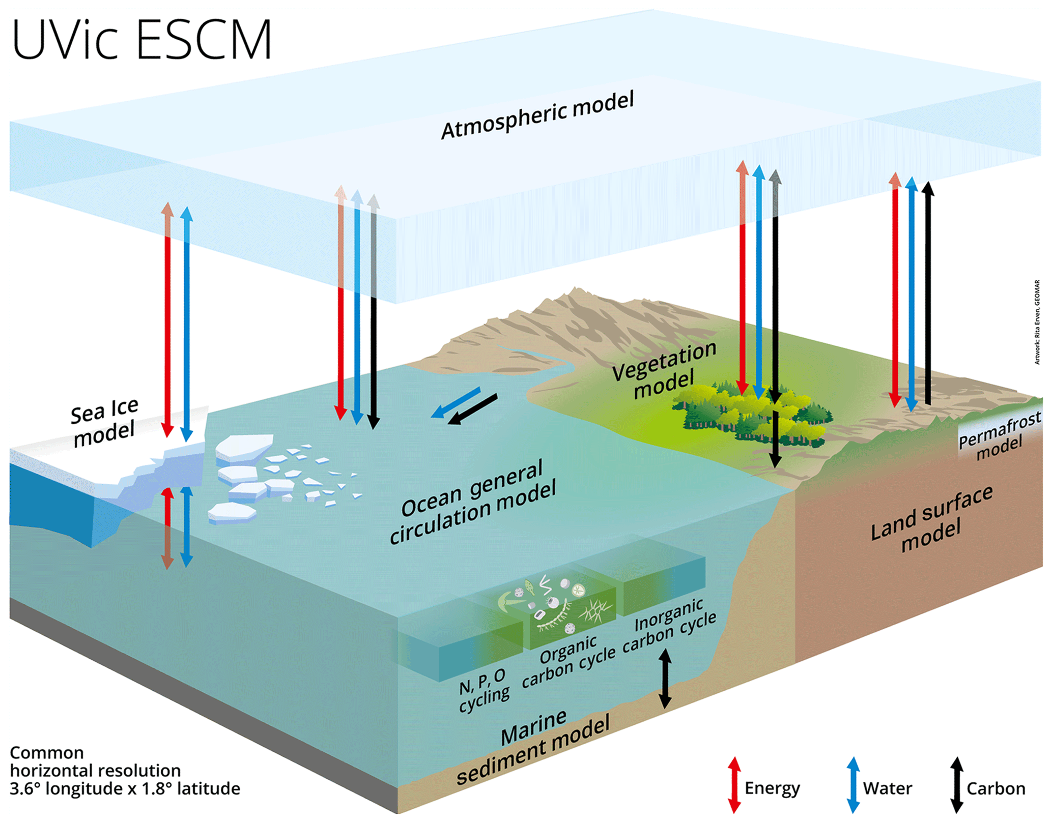
Figure 1Schematic of the University of Victoria Earth System Climate Model version 2.10 (UVic ESCM 2.10).
In addition, the terrestrial component represents vegetation dynamics including five different plant functional types (Meissner et al., 2003). Sediment processes are represented using an oxic-only calcium-carbonate model (Archer, 1996). Terrestrial weathering is diagnosed from the net sediment flux during spin-up and held fixed at the equilibrium pre-industrial value for transient simulations (Meissner et al., 2012). The new version 2.10 of the University of Victoria Earth System Climate Model (UVic ESCM) presented here brings together and combines multiple model developments and new components that have come about since the last official release of the model in the CMIP5 context. In the following, the novel model components are described in detail.
2.1.1 Marine biogeochemical model
The ocean biogeochemistry model as published by Keller et al. (2012) is novel compared to the 2009 version of the model. It now includes equations describing phytoplankton light limitation and zooplankton grazing, a more realistic zooplankton growth and grazing model, and formulations for an iron limitation scheme to constrain phytoplankton growth. In this context, the ocean's mixing scheme was changed from a Bryan–Lewis profile to a scheme for the computation of tidally induced diapycnal mixing over rough topography (Simmons et al., 2004) (see ocean diffusivity profiles in Fig. S3). In addition, the air to sea gas parameterization was updated following the ocean carbon-cycle model intercomparison project updates for these numbers (Wanninkhof, 2014), which impacts the carbon exchange between the atmospheric and marine components. Furthermore, we now apply the stoichiometry from Paulmier et al. (2009) to consistently account for the effects of denitrification and nitrogen fixation on alkalinity and oxygen.
2.1.2 Soil model
The terrestrial component has also been updated relative to the latest official release of the UVic ESCM. It now includes a representation of soil freeze–thaw processes resolved in 14 subsurface layers of which the thicknesses exponentially increase with depth: the surface layer having a thickness of 0.1 m, the bottom layer a thickness of 104.4 m and the total thickness of the subsurface layers being 250 m. The top eight layers (to a depth of 10 m) are soil layers; below this are bedrock layers having the thermal characteristics of granitic rock. Moisture undergoes free drainage from the base of the soil layers, and the bedrock layers are hydrologically inactive (Avis et al., 2011). In addition, the soil module includes a multi-layer representation of soil carbon (MacDougall et al., 2012). Organic carbon from the litter flux is allocated to soil layers as a decreasing function of depth and is only added to soil layers with a temperature above 1 ∘C. If all layers are below this temperature threshold, the litter flux is added to the top layer of soil. Soil respiration remains a function of temperature and moisture (Meissner et al., 2003) but is now implemented in each layer individually. Respiration ceases if the soil layer is below 0 ∘C. Soil carbon is present in the top six layers of the soil column down to a depth of 3.35 m.
2.1.3 Permafrost model
A representation of permafrost carbon has also been added to the model. Permafrost carbon is prognostically generated within the model using a diffusion-based scheme meant to approximate the process of cryoturbation (MacDougall and Knutti, 2016), which is to say a freeze–thaw generated mechanical mixing process that causes subduction of organic carbon rich soils from the surface into deeper soil layers in permafrost-affected soils. In model grid cells with perennially frozen soil layers, soil carbon is diffused proportional to the effective carbon concentration of each soil layer. Effective carbon concentration is carbon concentration divided by porosity and a saturation factor (MacDougall and Knutti, 2016). Carbon that is diffused into perennially frozen soil is reclassified as permafrost carbon and is given different properties from regular soil carbon. Permafrost carbon decays with its own constant decay rate and is subject to an “available fraction” which determines the fraction of permafrost carbon that is available to decay. The available fraction slowly increases if permafrost carbon becomes thawed and decreases if permafrost carbon decays. Using this scheme, the model can represent the large fraction of permafrost carbon that is in the passive soil carbon pool while still allowing the passive pool to eventually decay (MacDougall and Knutti, 2016).
2.2 Description of the CMIP6 forcing for the UVic ESCM
Anthropogenic forcing from greenhouse gases (GHGs), stratospheric and tropospheric ozone, aerosols, and stratospheric water vapour from methane oxidation is considered. Natural forcing includes solar and volcanic. All data used in the creation of this dataset can be accessed from input4MIP from the Earth System Grid Federation (ESGF) unless otherwise specified. In the following, we will briefly describe how the input data for our simulations with the University of Victoria Earth System Climate Model (UVic ESCM) were created.
In the standard CMIP6 configuration, the UVic ESCM is forced with CO2 concentration data (ppm) (Meinshausen et al., 2017) and then calculates the radiative forcing internally. These equations were updated to represent the newest findings from Etminan et al. (2016). In contrast to that, radiative forcing for non-CO2 GHGs was calculated externally and summed up to be used as an additional model input using concentration data of 43 GHGs (Meinshausen et al., 2017). We use updated radiative forcing formulations for CO2, CH4 and N2O following the findings of Etminan et al. (2016). Radiative forcing of other GHGs was calculated using the formulations in Table 8.A.1 from the IPCC's Fifth Assessment Report (IPCC AR5; Shindell et al., 2013). Meinshausen et al. (2017) introduced three options for calculating radiative forcing from GHG concentrations. For this study, we chose to use the option with which one uses specific calculations for all available 43 GHGs rather than treating some groups of GHGs in a similar manner.
The radiative forcing of stratospheric water vapour from methane oxidation was calculated following the suggestion from Smith et al. (2018) by multiplying CH4 effective radiative forcing by 12 %. To calculate radiative forcing of tropospheric ozone, , the equations from Smith et al. (2018) were used:
and
where β are the forcing efficiencies, are methane concentrations, EX are emissions of the respective species (NOx – nitrate aerosols, CO – carbon monoxide, NMVOC – non-methane volatile organic compounds), EX,pi are the respective pre-industrial constants for the specific species, and T is temperature in Kelvin. Note that f(T) was not included in our calculations because the forcing is not calculated dynamically. Concentrations and emissions data were obtained from input4MIPs from the Earth System Grid Federation. Pre-industrial values were taken from Table 4 from Smith et al. (2018). Again following Smith et al. (2018), radiative forcing of stratospheric ozone, , can be calculated from GHG concentration data using
with
where , , and c=1.03 are curve fitting parameters and rCFC11 is the fractional release values for trichlorofluoromethane. Equivalent stratospheric chlorine of all ozone depleting substances (ODSs) is represented by Eq. (4) as a function of ODS concentrations. The ri are fractional release values for each ODS as defined by Daniel and Velders (2011). There are no data provided for the ODS Halon 1202, which is accordingly not included in the calculation.
Three-dimensional aerosol optical depth (AOD) input for the UVic ESCM was created using a UVic ESCM grid and the scripts and data provided by Stevens et al. (2017), which describe nine plumes globally that are scaled with time to produce monthly sulfate aerosol optical depth forcing for the years 1850–2018 (for comparison see Fig. S1). The resulting AOD caused a forcing that was too strong in the historical period. Therefore, an option was implemented into the UVic ESCM which allows the user to scale the aerosol forcing from AOD data to fit it to current values. For transient simulations, the scaling factor was set to 0.7, which gives a globally average forcing of −1.04 W m−2 in 2014, consistent with the IPCC AR5 range estimate of between −1.9 and −0.1 W m−2 (Boucher et al., 2013; Myhre et al., 2013) and the newest updates of this forcing of W m−2 from Smith et al. (2020).
Anthropogenic land-use changes (LUCs) in the UVic ESCM are prescribed from standardized CMIP6 land-use forcing (Ma et al., 2020) that has been re-gridded onto the UVic grid. These gridded land-use data products (LUH2), which contain information on multiple types of crop and grazing lands, were adapted for use with UVic by aggregating the crop lands and grazing lands into a single “crop” type, which can represent any of five crop functional types, and a single “grazing” variable, which represents both pasture and rangelands. This forcing is used by the model to determine the fraction of each grid cell that is crop or grazing land, with those fractions of each terrestrial grid cell then assigned to C3 and C4 grasses and excluded from the vegetation competition routine of the Top-down Representation of Interactive Foliage and Flora Including Dynamics (TRIFFID) vegetation model. CO2 emissions from LUC affect the model runs so that when forest or other vegetation is cleared for crop lands, range lands or pasture, 50 % of the carbon stored in trees is released directly into the atmosphere, and the remaining 50 % is placed into the short-lived carbon pool.
Historical volcanic radiative forcing data are provided by Schmidt et al. (2018). Following CMIP6 spin-up forcing recommendations (Eyring et al., 2016), volcanic forcing is applied as an anomaly relative to the 1850 to 2014 period in the UVic ESCM.
Solar constant data for 1850 to 2300 were accessed from input4MIPs (Matthes et al., 2017). The available monthly data were annually averaged. Following CMIP6 spin-up forcing recommendations (Eyring et al., 2016), spin-up values were set to the mean of 1850–1873, which is equal to 1360.7471 W m−2.
A comparison of radiative forcing used for the UVic ESCM for Coupled Model Intercomparison Projects 5 and 6 (CMIP5 and CMIP6, respectively) and the data for the historical period as given by the IMAGE model (Meinshausen et al., 2011) is shown in Fig. S2. Even though the model has been fine tuned to reproduce the recent observational period while following the CMIP6 forcing data and protocols, the model is not limited to CMIP6 context applications.
2.3 Description of the CMIP6 forcing for the UVic ESCM
The model was spun up with boundary conditions as described in the CMIP6 protocol by Eyring et al. (2016) for over 10 000 years, in which the weathering flux was dynamically simulated and diagnosed. For all transient and diagnostic simulations, the weathering flux was then set as a constant to the value at the end of the spin-up of 8703 kg C s−1. To diagnose the transient climate response (TCR), equilibrium climate sensitivity (ECS), the ocean heat uptake efficiency (κ4x) and the transient climate response to cumulative emissions (TCREs), as given in Table 1, we ran 1000 year simulations starting with a 1 % yr−1 increase in CO2 concentrations until a doubling (2xCO2) and quadrupling (4xCO2) were reached after which the concentration was kept constant. Before switching from CO2-concentration-driven simulations to CO2-emissions-driven simulations, a 1500-year drift simulation was run. Finally, the historical simulation is forced with fossil CO2 emissions, dynamically diagnosed land-use change emissions, non-CO2 GHG forcing, sulfate aerosol forcing, volcanic anomalies forcing and solar forcing.
2.4 Fine tuning of the UVic ESCM 2.10
We tested version 2.10 of the UVic ESCM with the main incentive to improve its skill in simulating carbon fluxes, historical temperature trajectories and ocean tracers. While evaluating the model with available observational data, specific additional changes and updates were applied with respect to the UVic ESCM versions 2.9-02 (Eby et al., 2009) and 2.9-CE (Keller et al., 2014).
After merging the two model versions, the UVic ESCM's simulated historical cumulative land-use change emissions were close to zero since its pre-industrial vegetation closely resembled the pattern of plant functional types of today. In order to get a good representation of deforested biomass, we updated the vegetation parameterization to ensure that diagnosed historical land-use change carbon emissions agree with observational estimates from Le Quéré et al. (2018). During this process there was a trade-off between getting the right amount of LUC emissions and a good representation of present-day broadleaf trees in tropical areas. In the end, the representation of LUC emissions had the higher priority to be able to simulate emissions-driven simulations. To slightly mitigate the high broadleaf tree density, we then decreased the terrestrial CO2 fertilization by 30 % following Mengis et al. (2018) by adjusting the atmospheric CO2 concentration that is used by the terrestrial model component. This was done to reduce the overestimation of broadleaf tree vegetation especially in tropical areas which, in the real world, are limited by phosphorus (Camenzind et al., 2018). The broadleaf tree representation and the terrestrial carbon flux were improved by the scaling of the CO2 fertilization strength (see Sect. 3.1. and 3.2.); the terrestrial carbon fluxes are now in better agreement with the Global Carbon Budget 2018 by Le Quéré et al. (2018).
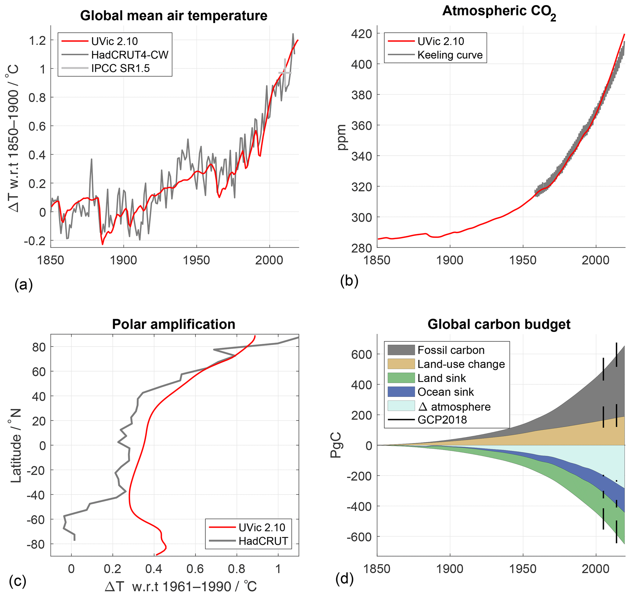
Figure 2(a) Global mean air temperature change for the UVic ESCM 2.10 relative to 1850–1900 (red line) in comparison with the average observed warming using the filled-in HadCRUT4-CW dataset from Haustein et al. (2017) (grey line) and the IPCC's special report on 1.5 ∘C GSAT temperature change for 2006–2015 (light grey cross). (b) Atmospheric CO2 concentrations in the UVic ESCM 2.10 (red line) in comparison with the Keeling curve from the Mauna Loa observatory (Keeling et al., 2005; grey line). (c) Zonal means of temperature change of the HadCRUT median near-surface temperature anomaly (grey line) (Morice et al., 2012) in comparison to the UVic ESCM 2.10. All temperature changes are for a 30-year mean around 1995 with respect to the 1961–1990 period (in K). (d) The global carbon budget for the UVic ESCM 2.10 partitioned into fossil fuel carbon, land-use carbon emissions, and atmosphere, land, and ocean sinks, compared to cumulative carbon fluxes between 1850 and 2005 and 1850 and 2015 from the Global Carbon Project 2018 (grey lines) (Le Quéré et al., 2018).
The new model version equilibrated with a rather low oceanic overturning strength; we therefore increased the ocean background vertical diffusivity from the previous value of 0.15 cm2 s−1 in Keller et al. (2014) to 0.25 cm2 s−1 to increase ocean overturning (see Figs. S3 and S4). This caused ocean diffusivity to slightly increase in depths between 0 and 3500 m relative to the previous model version (Fig. S3) but to follow the tidal mixing profile very closely for greater depths. Global diffusivity increased by about 4 %. This change enabled us to reach a very similar ocean overturning as found for the UVic ESCM 2.9-02, which uses the Bryan–Lewis mixing scheme (Figs. S3 and S4). This stronger overturning then in turn also improved ocean physical properties (see Sect. 3.3 and Supplement), as well as the global mean temperature and warming trends. However, it also causes the ocean heat content (OHC) anomaly for the upper 700 m to amount to 23.9×10²² J, which is an overestimation of the observed 700 m OHC anomaly of J (Levitus et al., 2012) (Table 1). This seems to be a general feature of Earth system models of intermediate complexity (EMICs) (Eby et al., 2013), but it might still be problematic. An overestimation in the change in the ocean heat content anomaly would, for example, result in a similar overestimation of thermosteric sea level change. Another possible impact of the overestimated ocean heat uptake can be the estimates of the Zero Emissions Commitment, which is directly linked to the state of thermal equilibration of the Earth system (Ehlert and Zickfeld, 2017; MacDougall et al., 2020). So the fact that EMICs in general, but the UVic ESCM 2.10 in particular, here overestimates the OHC anomaly trend has to be kept in mind if the model were to be used for experiments concerning this metric.
In this section, we evaluate the performance of the different components of the UVic ESCM version 2.10 based on observations.
Table 1Key global mean metrics of the UVic ESCM 2.10 compared to relevant observations or model intercomparison projects. The ΔT20th century is the change in surface air temperature over the 20th century from the historical “all” forcing experiment. TCR2xCO2, TCR_4xCO2 and ECS4xCO2 are the changes in global average model surface air temperature from the decades centered at years 70, 140 and 995, respectively, from the idealized 1 % increase to 4xCO2 experiment. The ocean heat uptake efficiency, κ4x, is calculated from the global average heat flux divided by TCR_4xCO2 for the decade centered at year 140 from the same idealized experiment. Note that ECS4xCO2 was calculated from the decade centered at year 995 from the idealized 1 % increase to 2xCO2 experiment.
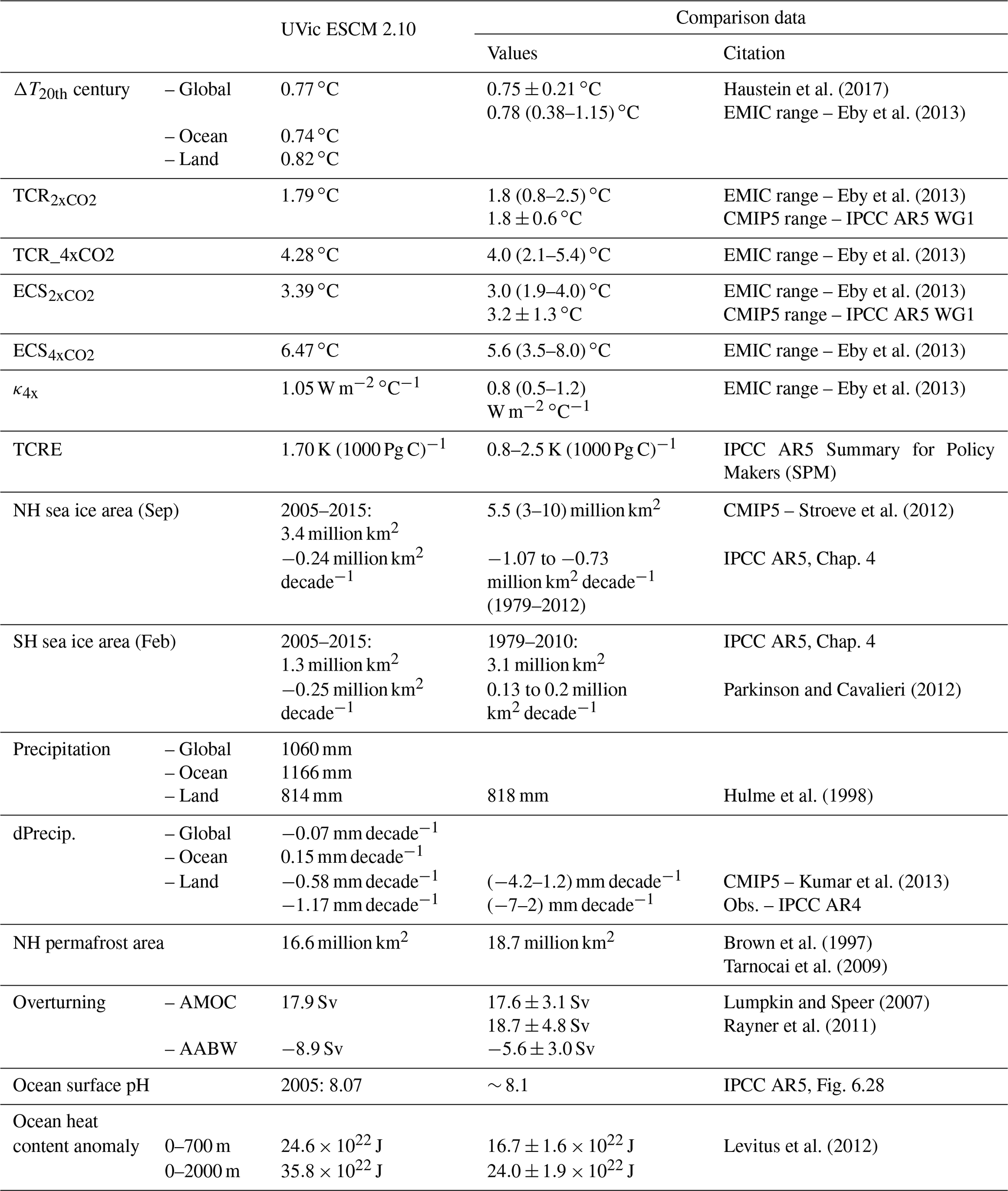
TCR – transient climate response, ECS – equilibrium climate response, κ4x – ocean heat uptake efficiency, TCRE – transient climate response to cumulative carbon emissions, NH – Northern Hemisphere, SH – Southern Hemisphere, AMOC – Atlantic meridional overturning, AABW – Antarctic bottom water.
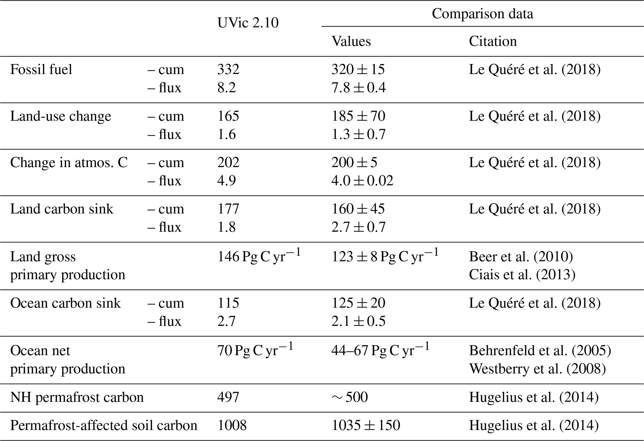
Table 2Global carbon cycle fluxes for the year 2005 (in Pg C yr−1) (– flux) or cumulated fluxes between 1850 and 2005 (in Pg C) (– cum) from the UVic ESCM 2.10 compared to data-based estimates from the Global Carbon Project 2018 and the IPCC AR5 Chap. 6. Note the observational estimates of the carbon stocks are calculated from 1750 to 2005.
3.1 Global key metrics – temperature, carbon cycle, climate sensitivity and radiation balance
The emissions-driven, transient historical climate simulation of the UVic ESCM version 2.10 forced with CMIP6 data reproduces well the historical temperature trend in the 20th century of 0.75±0.21 ∘C as derived from the Global Warming Index (Haustein et al., 2017) (Table 1; Fig. 2). Starting from the year 2000, the simulated global mean temperature increases at a higher rate than previously, but the total temperature change since pre-industrial times remains within the uncertainty range of the estimate in the latest IPCC special report on 1.5 ∘C (Fig. 1; light grey cross) (Rogelj et al., 2018). This steep temperature increase over the last 20 years of simulations amounts to a rate of temperature change of 0.27 ∘C decade−1, which is higher than the best estimate from the infilled HadCRUT4-CW dataset of 0.17 ∘C decade−1 (uncertainty range of 0.13–0.33 ∘C decade−1) (Haustein et al., 2017).
The simulated transient climate response (TCR) for a doubling and quadrupling of atmospheric CO2 concentration is 1.79 and 4.28 ∘C, respectively, and therefore well within the reported ranges from the EMIC comparison study by Eby et al. (2013). The main differences between model versions are the updated CO2 forcing formulation that was adopted from Etminan et al. (2016). For an atmospheric CO2 concentration of 1120 ppm (i.e. 4 times pre-industrial CO2), the new formulation gives a forcing of 8.08 W m−2 compared to the previous formulation implemented in the UVic ESCM that gave a forcing of 7.42 W m−2. In the same way, there is good agreement with the EMIC multi-model mean and the diagnosed values for the equilibrium climate sensitivity for a 2 times and 4 times increase in atmospheric CO2 concentrations with temperature increases of 3.39 and 6.47 ∘C, respectively. Since the ocean heat uptake efficiency is assessed at year 140 of the TCR4x simulation, it is, like the TCR4x, on the higher end with 1.05 W m−2 ∘C−1 but still within the EMIC range. In the same way, the transient climate response to cumulative emissions (TCRE) agrees well with previous model versions, with 1.70 ∘C (1000 Pg C)−1, and it remains within the likely range reported by the IPCC AR5 (Table 1).
Overall, the global carbon-cycle fluxes of the UVic ESCM 2.10 are within the uncertainty ranges of the Global Carbon Project (Le Quéré et al., 2018; GCP18) (Table 2; Fig. 2). The CO2 concentrations as simulated in the emissions-driven simulation follow the Keeling curve closely, but there is a slightly higher increase between 1960 and 2010 in the simulation with an increase of 77 ppm compared to the observations of 73 ppm. The change in atmospheric carbon between 1850 and 2005 is, however, within the uncertainty estimate of the GCP18 (Table 2). The land-use change emissions, which are generated dynamically in the model by changes in agriculturally used areas, reach a cumulative level of 165 Pg C between 1850 and 2005 and are hence well within the uncertainty range of the GCP18 estimate of 185±70 Pg C (Table 2). Both the cumulative ocean sink with 115 Pg C and the land sink with 177 Pg C in the period between 1850 and 2005 are within the uncertainty range of the GCP18 (Table 2). While the land sink is slightly higher than the best estimates, the ocean sink is at the lower end of the given range.
Table 3Global radiation balance of the UVic ESCM 2.10 in comparison with Wild et al. (2013). Unitless albedo values and radiation fluxes (in W m−2) are shown.
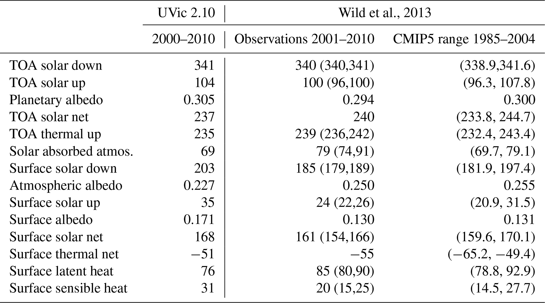
TOA – top of the atmosphere.
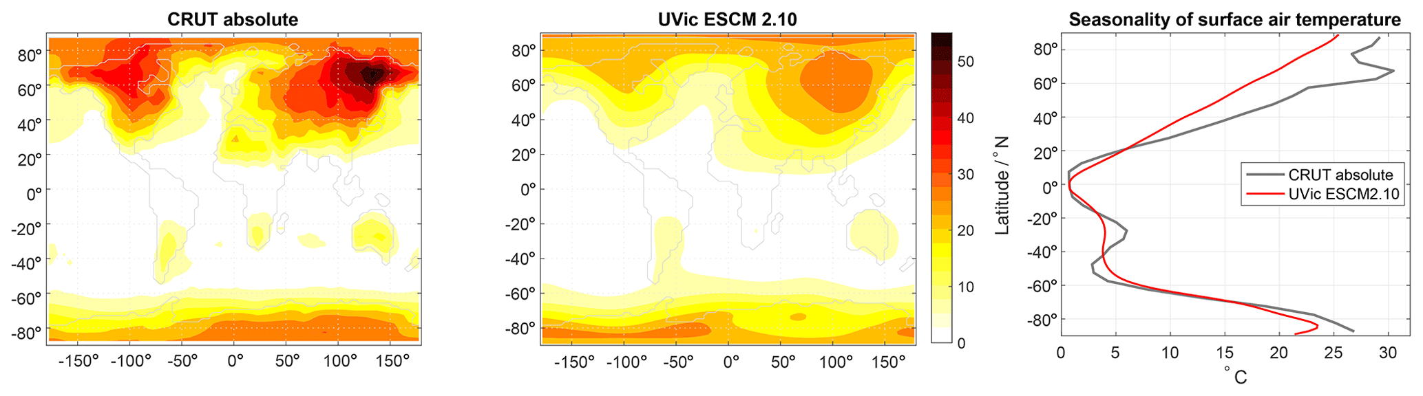
Figure 3Seasonality of surface air temperature as differences between December–January–February and June–July–August means for the Climate Research Unit global 1961–1990 mean monthly surface temperature climatology (Jones et al., 1999) and the UVic ESCM for the period of 2000–2005.
The simulated top of the atmosphere (TOA) short-wave and long-wave radiation of the UVic ESCM for the year 2005 lies well within the range of the CMIP5 models as reported by Wild et al. (2013) and agrees reasonably well with the observed estimates for both the solar and the thermal radiation fluxes (Table 3; Fig. S5). The same is true for the simulated net surface thermal flux, which is −51 W m−2 and therefore at the lower end of the CMIP5 range (Table 3). Now following the solar radiation through the energy moisture balance model, however, we find that the simulated atmospheric albedo of 0.227 is comparatively low to the observed value of 0.250. This causes the rather low simulated absorption of solar radiation by the atmosphere of 69 W m−2, for which the observed estimate from Wild et al. (2013) is 79 W m−2. Thanks to a rather high simulated surface albedo (0.171 compared to 0.130 from observations), the resulting absorbed solar radiation at the surface is still high, but, in contrast to the atmospheric absorption, it is within the CMIP5 range. This results in a global mean surface net radiation of 117 W m−2 which is rather high compared to the observed best estimate of 106 W m−2. This is the radiative energy available at the surface to be redistributed amongst the non-radiative surface energy balance components. Accordingly, the simulated sensible heat flux in the UVic ESCM of 31 W m−2 is also too high compared to the CMIP5 range of 14.5 to 27.7 W m−2. Finally, the latent heat flux calculated from simulated evaporation of 76 W m−2 is on the very low end of observational and CMIP5 estimates, which is likely linked to the high transpiration sensitivity of plants in the UVic ESCM (Mengis et al., 2015).
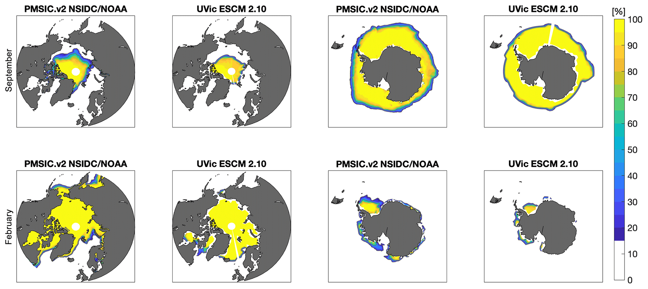
Figure 4September (top row) and February (bottom row) sea ice concentrations from passive microwave observations (Meier et al., 2013) and the UVic ESCM 2.10 for the Northern Hemisphere and Southern Hemisphere for the period of 2003–2013 (in %).
3.2 Spatially resolved atmospheric and land surface metrics
The simulated polar amplification of the UVic ESCM 2.10 compares well to the HadCRUT near-surface temperature anomaly data for all latitudes except for the Southern Ocean south of 40∘ S (Fig. 2). Here the UVic ESCM 2.10 shows more of a warming trend than what is observed. Previous studies have shown that this warming is connected to the representation (or the lack thereof) of poleward-intensified winds (Fyfe et al., 2007). This warming trend was already evident in previous versions of the UVic, as well as in other EMICs (see Fig. S6 and Fig. 4 in Eby et al., 2013). While the pattern of the seasonal cycle concerning surface air temperature agrees well with the Climate Research Unit (CRU) global 1961–1990 mean monthly surface temperature climatology (Fig. 3), the magnitude, especially in the Northern Hemisphere land areas, is substantially lower by up to 25 ∘C, which is also reflected in the latitudinal means.
The simulated Northern Hemisphere summer sea ice extent with 3.4 million km−2 is at the lower end of the CMIP5 estimates and considerably smaller than the observed sea ice concentration (Table 1; Fig. 4). This lower extent seems to be mainly due to a lack of simulated summer sea ice concentrations between 15 % and 60 %, whereas higher concentrations show good agreement with the observed pattern (Fig. 4). The southward extension of the winter sea ice concentration in the UVic ESCM is considerably smaller than the observations from passive microwave satellite missions. Concerning Northern Hemisphere (NH) summer sea ice trends, the UVic ESCM shows lower trends of −0.24 million km−2 decade−1 during the last 30 years, compared to what is observed (−1.07 to −0.73 million km−2 decade−1) (IPCC AR5, Chap. 4; Ciais et al., 2013). The summer sea ice extent in the Southern Hemisphere of 1.3 million km−2 is also smaller than the observed 3.1 million km−2 and, in contrast to the observed increasing trends in sea ice, shows a decline of −0.25 million km2 decade−1 (Table 1). While this is consistent with the simulated warming trend in the Southern Hemisphere surface air temperature, this is still a bias in the model.
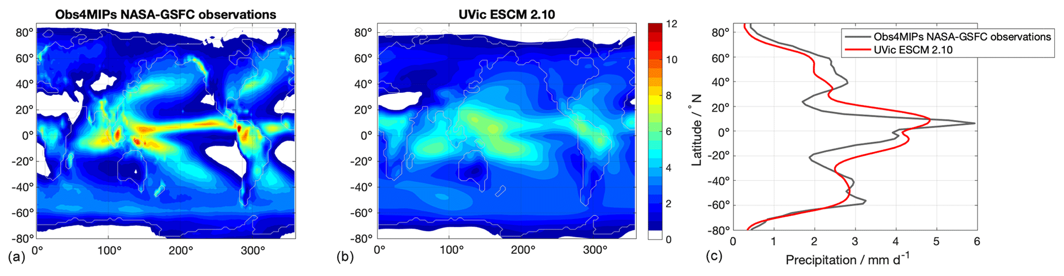
Figure 5Mean precipitation flux for the period 1979–2013 (in mm d−1) from Obs4MIP (Adler et al., 2003) (a; grey line in c) and the UVic ESCM 2.10 (b; red line in c), and zonally averaged values as a function of latitude (c).
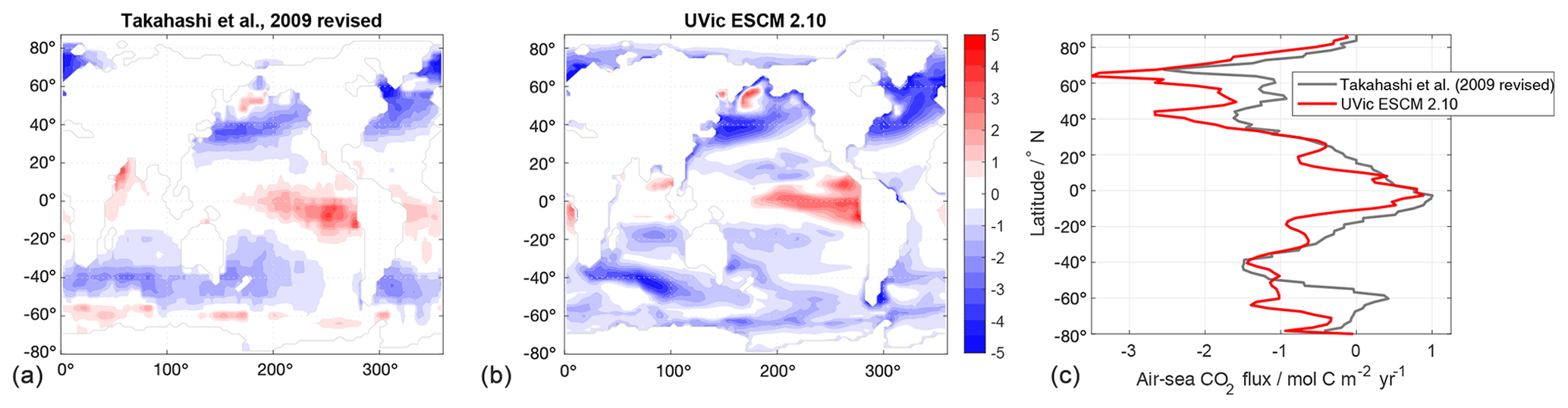
Figure 6Air–sea carbon flux for the year 2005 (in mol C m−2 yr−1) from the revised dataset from Takahashi et al. (2009) (a; grey line in c) and the UVic ESCM 2.10 (b; red line in c). Zonally averaged values as a function of latitude (c).

Figure 7Vegetation carbon density for the 1960–2000 period (in kg C m−2) from the revised CDIAC NDP-017 dataset (Olson et al., 2001) (a; grey line in c) and the UVic ESCM 2.10 (b; red line in c). Zonally averaged values as a function of latitude (c).
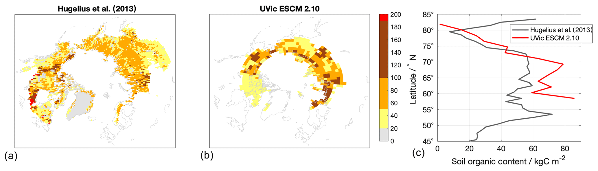
Figure 8Soil organic carbon content in permafrost-affected soils for the 1980–2000 period in the top 3 m of soil (in kg C m−2) from the dataset by Hugelius et al. (2014) (a) and for the UVic ESCM 2.10 (b). Zonally averaged values as a function of latitude (c).
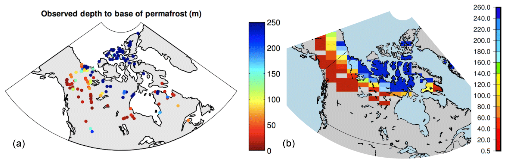
Figure 9Observed depth of permafrost for the region of northern Canada (a) (data source: Smith and Burgess, 2002; figure source: Avis, 2012). The colour bar has been restricted to 250 m depth to aid in comparison despite the fact that many locations are deeper (Avis, 2012). Simulated mean permafrost depth for 1966–1990 of the UVic ESCM 2.10 (b).
Observed global mean terrestrial precipitation between 1961 and 1990 amounts to 818 mm (Hulme et al., 1998). The adjusted CO2 fertilization strength in the UVic ESCM 2.10 results in global mean terrestrial precipitation of 814 mm for the same period (Table 1), bringing it close to the observed amount. Concerning terrestrial precipitation trends, the UVic ESCM 2.10 shows a negative trend in terrestrial precipitation of −0.58 mm decade−1 for the period between 1930 and 2004 (Table 1). This is in agreement with the range of terrestrial precipitation trends of −4.2–1.2 mm decade−1 given by Kumar et al. (2013). The terrestrial precipitation trend of −1.17 mm decade−1 also agrees well with the observed terrestrial precipitation changes for the recent historical period (1951–2005) of −7 to +2 mm decade−1, with error bars ranging from 3 to 5 mm decade−1 (IPCC AR4) (Table 1). The simulated pattern of annual mean precipitation flux for the last 30 years generally agrees well with the observed pattern (Fig. 5). Similar to the seasonal temperature maps, the UVic ESCM slightly underestimates the most extreme amplitudes of annual mean precipitation located in the tropical areas. The latitudinal mean values agree well in magnitude, but the tropical rain bands are extending too far north and south.
The simulated air–sea carbon flux for 2000 to 2010 agrees with observations from Takahashi et al. (2009) (Fig. 6). Oceanic carbon uptake takes place at high latitudes, and carbon is mainly released in the tropical Pacific. In the Southern Ocean, observations show slightly positive values (i.e. carbon being released to the atmosphere) which are not reproduced by the UVic ESCM 2.10. This is also evident in the latitudinal means, in which the UVic ESCM 2.10 generally shows good agreement with the observations but simulates ocean carbon uptake south of 50∘ S, where the observations show low uptake or even a small carbon release.
The UVic ESCM overestimates vegetation carbon density in tropical rainforest regions, such as in South America and central Africa, when compared to the revised estimates of Olson (1983, 1985, 2001) (Fig. 7). More recent biomass studies have challenged Olson's estimates for some regions of the world, but Olson (1983, 1985) still provides the only globally consistent estimate of global carbon stored in vegetation. This positive bias in the UVic ESCM 2.10 in the tropics is due to an overestimation of broadleaf trees, which is the plant functional type with the highest carbon density in the UVic ESCM (see Fig. S7). This overestimation of broadleaf trees leads to a small overestimation of global mean gross primary production in 2005 on land, 146 Pg C yr−1, compared to the observation-based estimate of 123±8 Pg C yr−1 using eddy covariance flux data and various diagnostic models (Beer et al., 2010) (Table 2). In contrast, the simulated vegetation coverage of carbon densities of 2–5 kg C m−2 is lower than observations especially in central Asia and at higher northern latitudes. This, however, does not imply that the dominant plant functional types, namely C3/C4 grasses, are underrepresented in this area. In the UVic ESCM 2.10, the representation of C3/C4 grasses, as well as needleleaf trees, in high northern latitudes improved compared to earlier versions (see Fig. S7) thanks to the more complex soil module and the corresponding vegetation tuning. In summary, the UVic ESCM overestimates broadleaf tree cover in the tropics but improved the representation of the vegetation cover at latitudes north of 20∘ N compared to previous model versions.
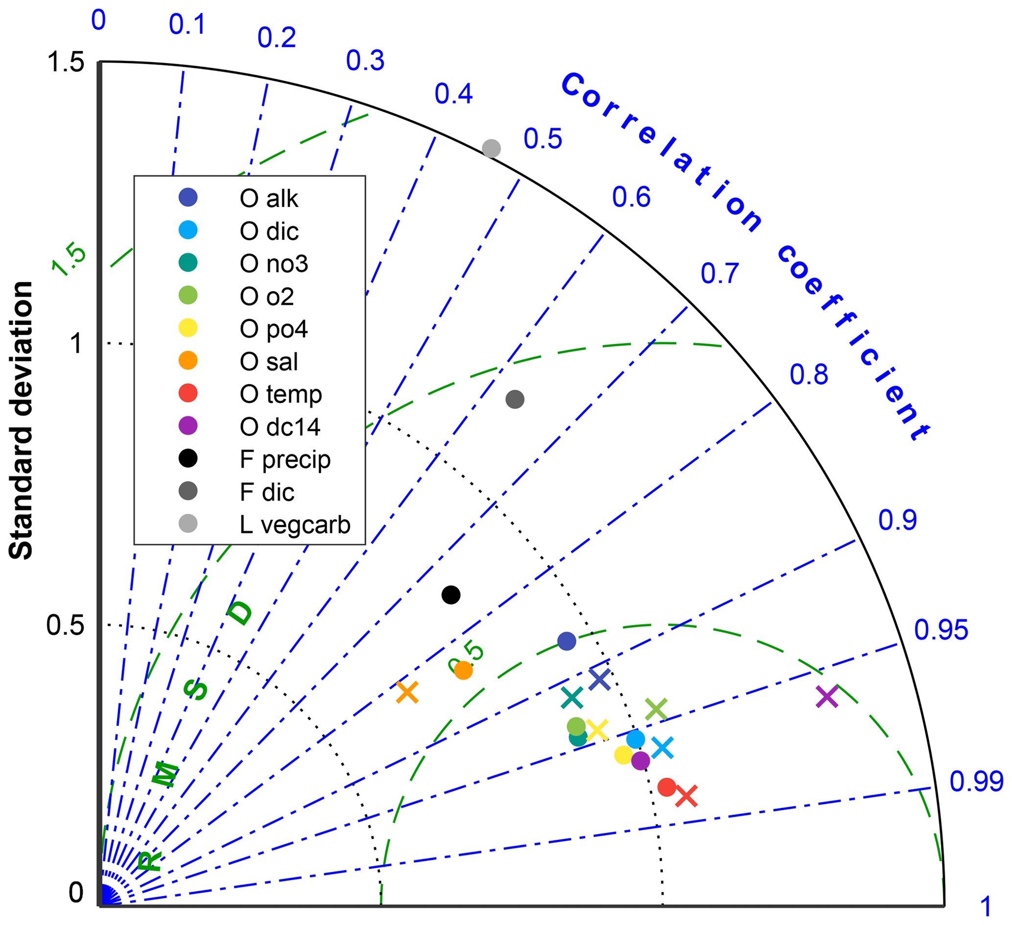
Figure 10Taylor diagram (Taylor, 2001) of multiple global UVic ESCM 2.10 fields (dots) and the UVic ESCM 2.9 fields (×) with respect to re-gridded observations from the World Ocean Atlas 2018 (Locarnini et al., 2018; Zweng et al., 2019; Garcia et al., 2018a, b), Global Ocean Data Analysis Project (GLODAP) and GLODAP mapped climatologies v2.2016b (Key et al., 2004; Lauvset et al., 2016), NASA-GSFC precipitation (Adler et al., 2003), air–sea gas fluxes from Takahashi et al. (2009), and vegetation carbon data from the CDIAC NDP-017 dataset (Olson et al., 2001). All datasets are normalized by the standard deviation of the observations. A perfect model with zero root mean square deviation, a correlation coefficient of 1 and a normalized standard deviation of 1 would plot at (1,0).
Simulated soil carbon densities at high northern latitudes compare reasonably well with the map of permafrost soil carbon based on observations by Hugelius et al. (2014) (Fig. 8). While there are regional biases especially in eastern Canada, the simulated carbon densities in the permafrost areas do have the correct order of magnitude. The total global permafrost carbon of 497 Pg C and the total soil carbon in the permafrost region of 1009 Pg C agree well with the reported ∼ 500 Pg C and 1035±150 Pg C, respectively (Hugelius et al., 2014). The simulated permafrost area is limited to about 60∘ N and does not extend as far south as what is observed.
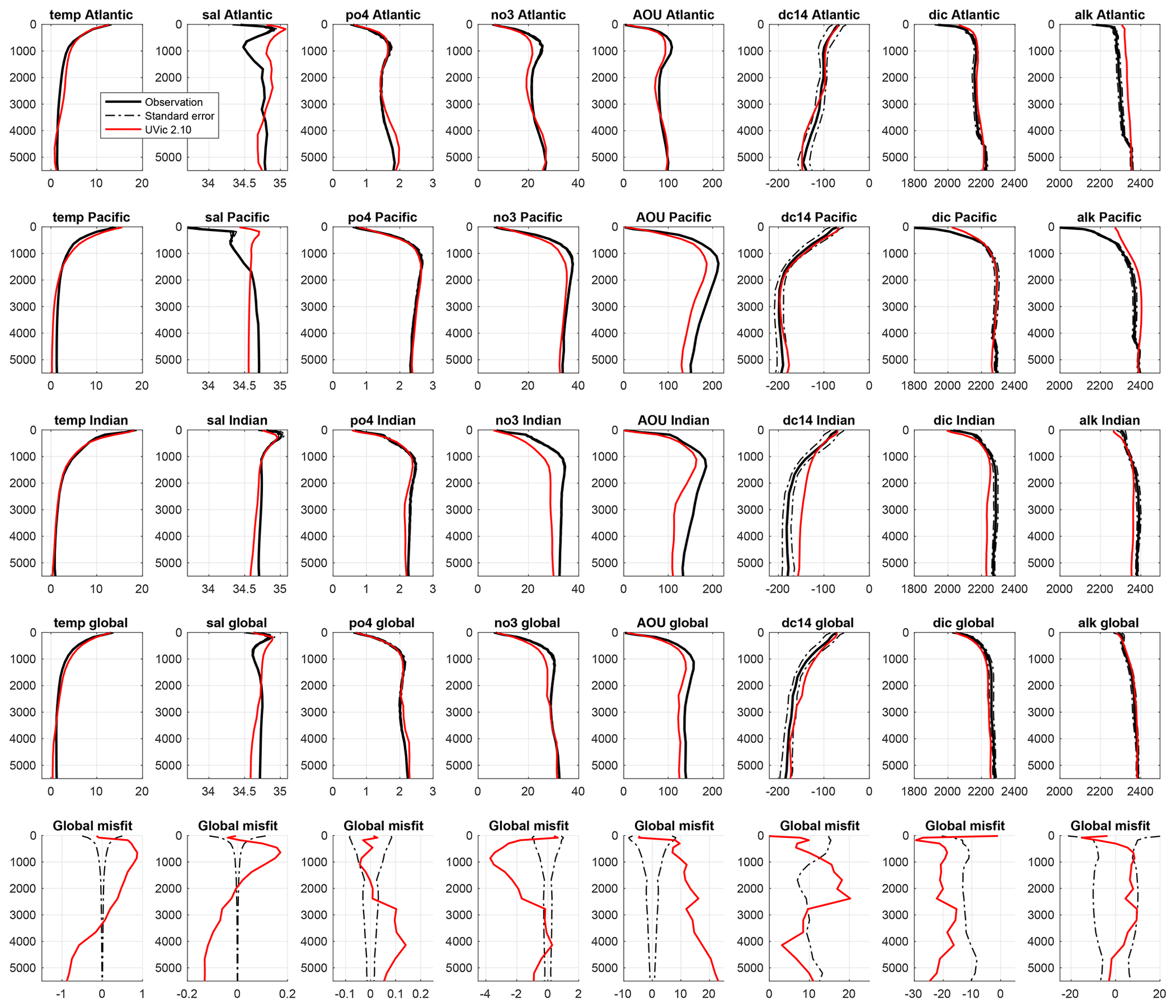
Figure 11Global and basin-wide averaged vertical profiles of multiple UVic ESCM 2.10 metrics (red lines) compared to observations from the World Ocean Atlas 2018 (Locarnini et al., 2018; Zweng et al., 2019; Garcia et al., 2018a, b) and GLODAP and GLODAP mapped climatologies v2.2016b (Key et al., 2004; Lauvset et al., 2016), including standard errors (solid and dashed black lines, respectively) and their respective global misfit (last row) for the period of 1980–2010. Note that for salinity we excluded the fresh water masses observed in the Arctic Ocean (i.e. all values north of 70∘ N for both datasets).
Smith and Burgess (2002) provide a dataset of permafrost depth observations for Canada based on temperature readings, which is a compilation of borehole data across Canada ranging in observational dates from between 1966 and 1990. Each borehole is a single observed value; this compares the simulation to a snapshot in time rather than a temporal average. Permafrost depth in the observational dataset was determined based on the bottom boundary identified by the temperature gradient to be below 0 ∘C. Permafrost depth distribution in North America simulated by the UVic ESCM broadly agrees with the observed distribution (Fig. 9). The UVic ESCM 2.10 simulates permafrost thicknesses of up to 250 m all around the Arctic circle. Recall that the depth of the UVic ESCM is limited to 250 m and that the vertical resolution is coarser at deeper soil layers. As already seen for the soil organic carbon content, the simulated permafrost areas do not extend as far south as what is observed. However, for the purpose of this comparison, the scale for observed permafrost depths was limited to 250 m, whereas actually many observations show deeper permafrost thicknesses.
3.3 Ocean metrics – physical and biogeochemical
In the following section, we will compare simulated ocean metrics with observations from the World Ocean Atlas 2018 (WOA18) (Locarnini et al., 2018; Zweng et al., 2019; Garcia et al., 2018a, b) and the Global Ocean Data Analysis Project (GLODAP) and the new mapped climatologies version 2 (Key et al., 2004; Lauvset et al., 2016) for the period of 1980 to 2010.
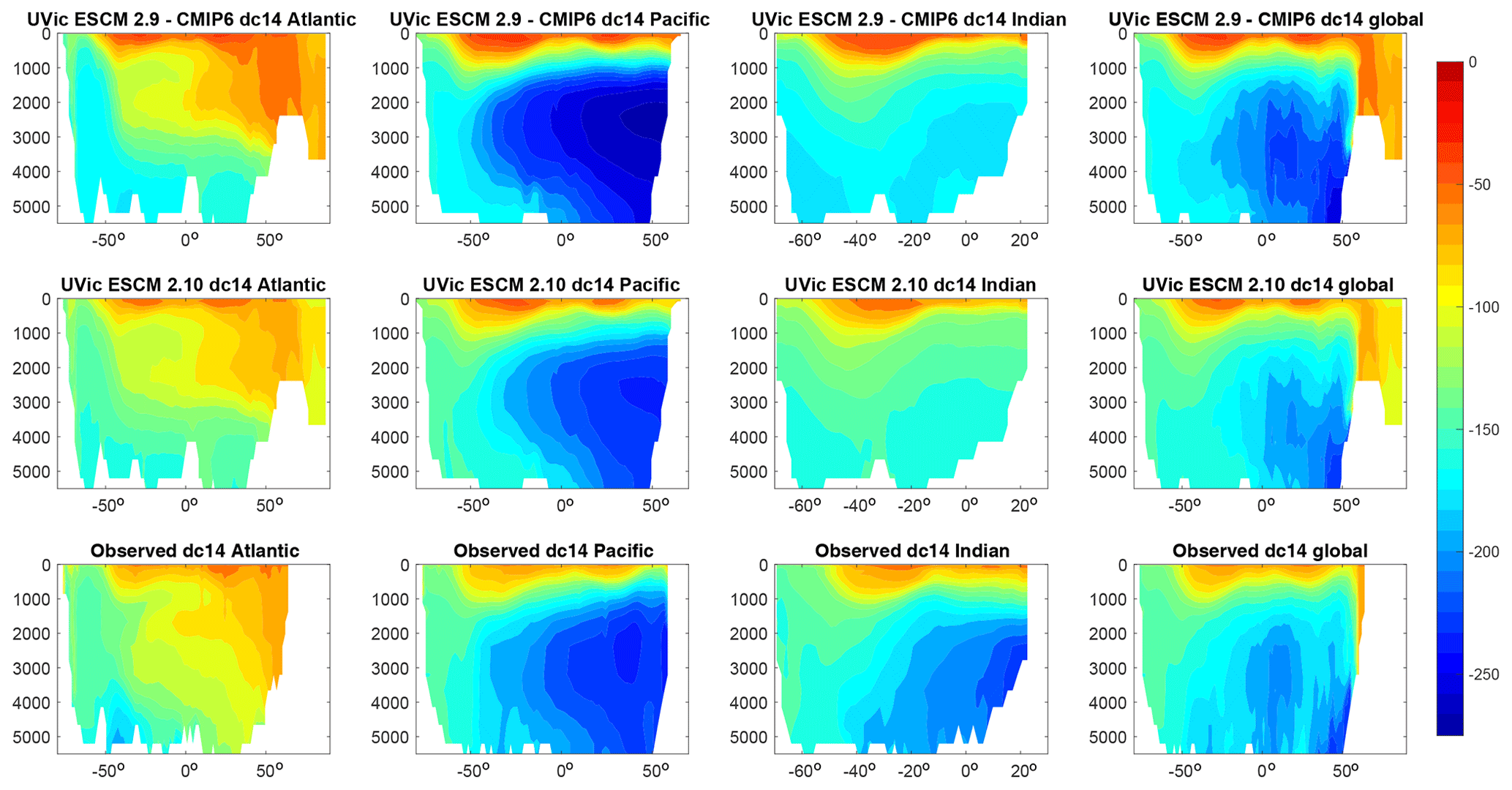
Figure 12Ocean section of ΔC14 (in ‰) for the Atlantic Ocean including the Arctic Ocean (left column), the Pacific Ocean (middle left column), the Indian Ocean (middle right column) and the global average (right column) compared to observations (Key et al., 2004). From top to bottom, what is shown are the published UVic ESCM version 2.9 by Eby et al. (2013) spun up and forced with CMIP6 forcing, the UVic ESCM version 2.10, both as a mean of the period 1980–2010, and the observed ocean sections.
The Taylor diagram for eight different ocean metrics illustrates that the UVic ESCM 2.10 improves ocean ΔC14 and slightly improves ocean temperature, salinity, and nitrate and phosphate distributions (dots in Fig. 10) relative to the UVic ESCM 2.9 (crosses in Fig. 10) given the same forcing. In contrast, mainly ocean alkalinity but also dissolved inorganic carbon and oxygen show either a larger deviation or lower correlation compared to observations than the previous model version. Generally, the model demonstrates skill in simulating these ocean properties with correlation coefficients higher than 0.9 for all but the salinity and alkalinity fields and a root mean square deviation (rmsd) of below 50 % of the global standard deviation of the observations – again with the exception of salinity and alkalinity. In the following, we will discuss these features in more detail.
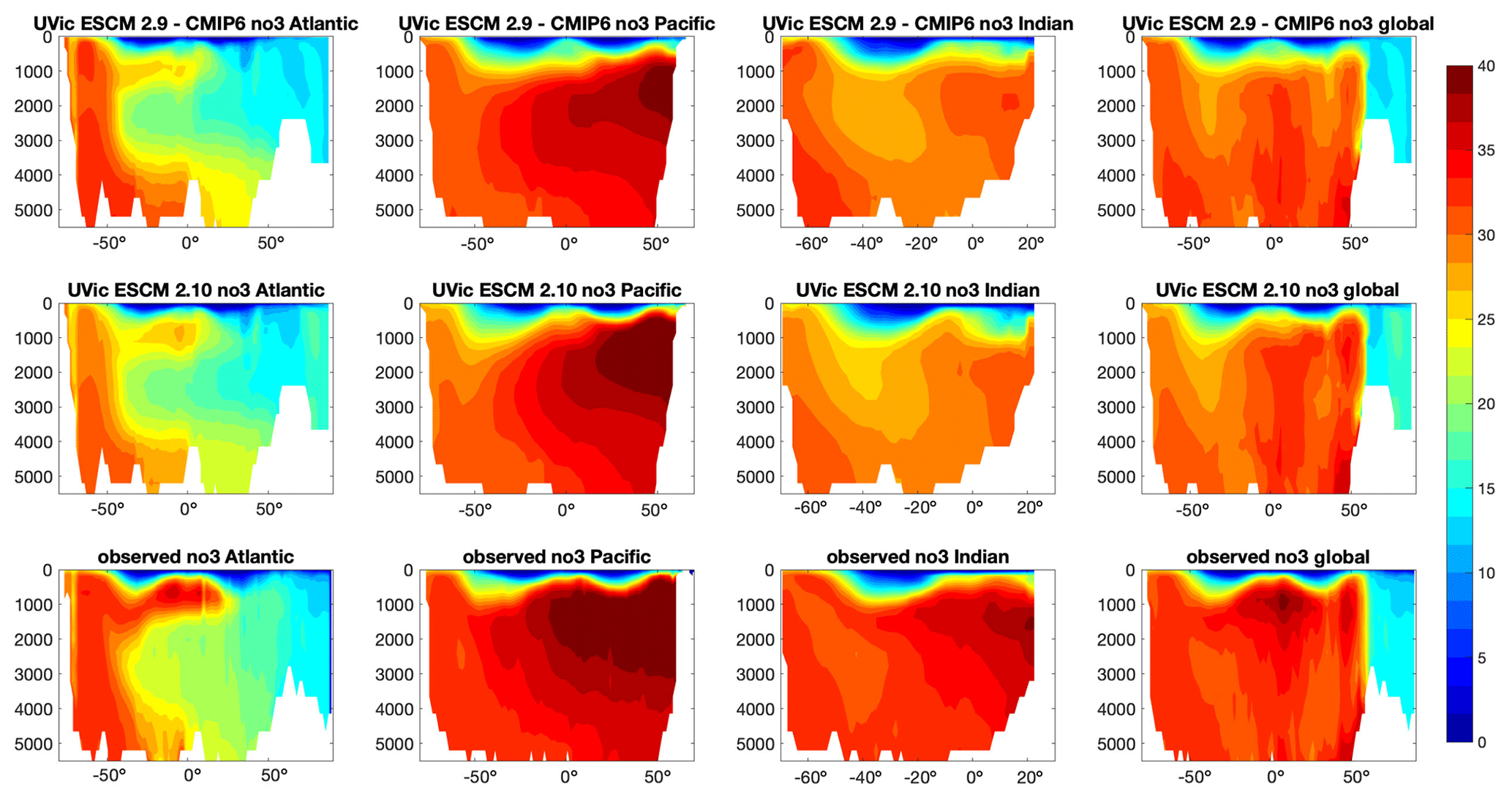
Figure 13Ocean section of NO3 (in µmol kg−1) for the Atlantic Ocean including the Arctic Ocean (left column), the Pacific Ocean (middle left column), the Indian Ocean (middle right column) and the global average (right column) compared to the World Ocean Atlas 2018 (Garcia et al., 2019). From top to bottom, what is shown are the published UVic ESCM version 2.9 by Eby et al. (2013) spun up and forced with CMIP6 forcing, the UVic ESCM version 2.10, both as a mean of the period 1980–2010, and the observed ocean sections.

Figure 14Maps of sea surface salinity (in practical salinity units; psu) for the published UVic ESCM version 2.9 (Eby et al., 2013) spun up and forced with CMIP6 forcing, for the UVic ESCM 2.10, and for the World Ocean Atlas 2018 (Zweng et al., 2019).

Figure 15Ocean section of apparent oxygen utilization (AOU) (in µmol kg−1) for the Atlantic Ocean including the Arctic Ocean (left column), the Pacific Ocean (middle left column), the Indian Ocean (middle right column) and the global average (right column) compared to the World Ocean Atlas 2018 (Garcia et al., 2019). From top to bottom, what is shown are the published UVic ESCM version 2.9 by Eby et al. (2013) spun up and forced with CMIP6 forcing, the UVic ESCM version 2.10, both as a mean of the period 1980–2010, and the observed ocean sections.
The vertical profiles of simulated temperature (temp), phosphate (PO4), nitrate (NO3), ΔC14, dissolved inorganic carbon (dic) and alkalinity (alk) agree well in magnitude and shape with the observed profiles for all ocean basins and the global ocean (Fig. 11). The general good agreement for these ocean metrics is also seen in comparisons with vertical ocean sections and ocean surface maps of these simulated fields with observations (see Supplement). The only noteworthy biases are ΔC14 that is too low in the central Indian Ocean basin, indicating an overturning rate that is too low in this ocean basin (see Figs. 11 and 12), and small biases in simulated nitrate showing values in the Arctic Ocean that are too high compared to observations and values in the Indian Ocean that are too low (see Figs. 11 and 13 and Supplement).
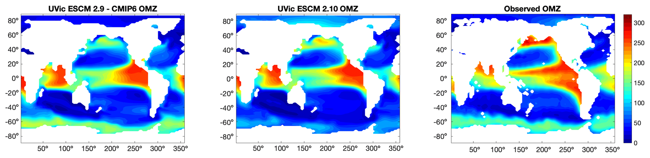
Figure 16Maps of apparent oxygen utilization in approx. 300 m depth (i.e. the depth of oxygen minimum zones, OMZs; in µmol kg−1) for the published UVic ESCM version 2.9-02 (Eby et al., 2013) spun up and forced with CMIP6 forcing, for the UVic ESCM 2.10, and for the World Ocean Atlas 2018 (Garcia et al., 2019).
To compare ocean salinity profiles (Fig. 11 second column), we removed values in the high northern latitudes, north of 70∘ N, for all regarded datasets. This substantially improved the comparison for the Atlantic Ocean (which in the partitioning includes the Arctic Ocean; see Supplement) since the UVic ESCM 2.10 does not reproduce well the recent freshening trend associated with sea ice loss and seasonal melt in the Arctic Ocean. The maps of sea surface salinity clearly show this freshening trend (Fig. 14), which also extends to the Pacific Ocean and is hence evident in the vertical profile (Fig. 11). Furthermore, the UVic ESCM 2.10 does not reproduce the salinity properties of Antarctic Intermediate Water (AAIW) well, which can be seen by the lack or insufficient representation of the local minimum in about 900 m depth for the global and Atlantic profile (see Supplement for latitudinal average sections). Note that the global mean temperature misfit shows similar patterns (Fig. 11). The bias in AAIW salinity in the UVic ESCM 2.10 is caused by surface waters that are too salty extending southward into the Southern Ocean regions, in which the water is subducted.
The apparent oxygen utilization (AOU) shows lower values (∼ 15 % lower) in the deep ocean but otherwise reproduces the shape including the local maximum around 1000 m depth well (Figs. 11 and 15). The main bias in AOU is found in the Southern Ocean, where the UVic ESCM 2.9 simulated values that were too high and the UVic ESCM 2.10 now simulates oxygen utilization values that are too low. This is especially true for the Atlantic and Indian oceans. These biases in AOU are probably linked to biases in the ocean biogeochemistry in the Southern Ocean. Comparing the simulated oxygen minimum zones (OMZs) of the UVic ESCM 2.9 and UVic ESCM 2.10 to observed OMZs, there is an improved representation of the asymmetry of the Pacific OMZ in the newer model version, as well as a reduced bias in the Indian Ocean (Fig. 16).
In order to obtain a new version of the University of Victoria Earth System Climate Model (UVic ESCM) that is to be part of the comparison of Earth system models of intermediate complexity (EMICs) in the sixth phase of the Coupled Model Intercomparison Project (CMIP6), we have merged previous versions of the UVic ESCM to bring together the ongoing model development of the last decades. In this paper, we evaluated the model's performance with regard to a realistic representation of carbon and heat fluxes, as well as ocean tracers, in the UVic ESCM 2.10 in agreement with the available observational data and with current process understanding.
We find that the UVic ESCM 2.10 is capable of reproducing changes in historical temperature and carbon fluxes. There is a higher warming trend in the Southern Hemisphere south of 40∘ S compare to observations, which causes a bias in Southern Hemisphere (SH) sea ice trends. The simulated seasonal cycle of global mean temperature agrees well with the observed pattern but has a lower amplitude especially in the high northern latitudes. The air to sea fluxes of the UVic ESCM agree well with the observed pattern. The newly applied CO2 forcing formulation has increased the model's climate sensitivity. Land carbon stocks concerning permafrost and vegetation carbon are within observational estimates even though the spatial distribution of permafrost-affected soil carbon and vegetation carbon densities show regional biases. The top of the atmosphere radiation balance of the UVic ESCM is well within the observed ranges, but the internal heat fluxes show biases. The simulated precipitation pattern shows good agreement with observations but is regionally too spread out especially in the tropics and, as expected, does not reach the most extreme values. Terrestrial total precipitation and precipitation trends agree well with observations. Many ocean properties and tracers show good agreement with observations. This is mainly caused by a good representation of the general circulation, although problems remain, mainly the Southern Ocean oxygen utilization being too low and the salinity bias in the AAIW.
These model data deviations, especially for the ocean tracers, have not yet been fully addressed (note the misfits have been reduced relative to the previous model version forced with new forcing) since we are already planning for the next update of the UVic ESCM, which will incorporate more comprehensive biogeochemical modules that will require the re-tuning of the oceans biogeochemical parameters as well. Model developments that have not been incorporated in the model version described here, like carbon-nitrogen feedbacks on land (Wania et al., 2012), explicit representation of calcifiers in the ocean (Kvale et al., 2015), the dynamic phosphorus cycle in the ocean (Niemeyer et al., 2017) and others, will in the following be implemented and tested within this new model version.
The model code and data shown in the figures and used for this paper are available at https://hdl.handle.net/20.500.12085/c565622a-9655-42bc-840c-c20e7dfd0861 (last access: 31 August 2020, GEOMAR OPeNDAP Service, 2020) and will also be made available on the official UVic ESCM webpage (http://terra.seos.uvic.ca/model/, last access: 31 August 2020), including all necessary documentation and data, upon final publication of the paper.
The supplement related to this article is available online at: https://doi.org/10.5194/gmd-13-4183-2020-supplement.
All authors decided on the content of the new model version; DPK merged the model code; DPK, NW, KZ, and NM compiled the CMIP6 forcing input; NM tuned it in consultation with AO, ME, AM, KM, AS, HDM, and KZ. NM and AJM ran the simulations for this publication, and NM wrote the paper with contributions from all authors.
The authors declare that they have no conflict of interest.
The authors would like to acknowledge Claude-Michel Nzotungicimpaye for his helpful discussions about soil hydrology and carbon context; Karin Kvale, Christopher Somes, and Wolfgang Koeve for their help looking at ocean alkalinity; and Heiner Dietze for his help with setting up the Fortran compiler.
Nadine Mengis was supported by the Natural Sciences and Engineering Research Council of Canada Discovery Grant (NSERC) awarded to Kirsten Zickfeld and the Helmholtz Initiative for Climate Adaptation and Mitigation (HI-CAM). The Helmholtz Climate Initiative (HI-CAM) is funded by the Helmholtz Association's Initiative and Networking Fund. Alex MacIsaac received support from the Natural Sciences and Engineering Research Council of Canada (NSERC) Discovery Grant awarded to Kirsten Zickfeld. Katrin J. Meissner received funding from the Australian Research Council (grant nos. DP180100048 and DP180102357). Andrew MacDougall was supported by the Natural Sciences and Engineering Research Council of Canada Discovery Grant program.
The article processing charges for this open-access
publication were covered by a Research
Centre of the Helmholtz Association.
This paper was edited by Steven Phipps and reviewed by two anonymous referees.
Adler, R. F., Huffman, G. J., Chang, A., Ferraro, R., Xie, P. P., Janowiak, J., Rudolf, B., Schneider, U., Curtis, S., Bolvin, D., Gruber, A., Susskind, J., Arkin, P., and Nelkin, E.: The version-2 global precipitation climatology project (GPCP) monthly precipitation analysis (1979–present), J. Hydrometeorol., 4, 1147–1167, https://doi.org/10.1175/1525-7541(2003)004<1147:TVGPCP>2.0.CO;2, 2003.
Archer, D.: A data-driven model of the global calcite lysocline, Global Biogeochem. Cy., 10, 511–526, https://doi.org/10.1029/96GB01521, 1996.
Avis, C. A., Weaver, A. J., and Meissner, K. J.: Reduction in areal extent of high-latitude wetlands in response to permafrost thaw, Nat. Geosci., 4, 444–448, https://doi.org/10.1038/ngeo1160, 2011.
Avis, C. A.: Simulating the Present-Day and Future Distribution of Permafrost in the UVic Earth System Climate Model, PhD thesis, University of Victoria, 2012.
Bagniewski, W., Meissner, K. J., and Menviel, L.: Exploring the oxygen isotope fingerprint of Dansgaard-Oeschger variability and Heinrich events, Quat. Sci. Rev., 159, 1–14, https://doi.org/10.1016/j.quascirev.2017.01.007, 2017.
Beer, C., Reichstein, M., Tomelleri, E., Ciais, P., Jung, M., Carvalhais, N., Rödenbeck, C., Altaf, M. A., Baldocchi, D., Bonan, G. B., Bondeau, A., Cescatti, A., Lasslop, G., Lomas, A. L. M., Luyssaert, S., Margolis, H., Oleson, K. W., Roupsard, O., Veenendaal, E., Viovy, N., Williams, C., Woodward, F. I., and Papale, D.: Terrestrial Gross Carbon Dioxide Uptake: Global Distribution and Covariation with Climate, Science, 329, 834–839, 2010.
Behrenfeld, M. J., Boss, E., Siegel, D. A., and Shea, D. M.: Carbon-based ocean productivity and phytoplankton physiology from space, Global Biogeochem. Cy., 19, GB1006, https://doi.org/10.1029/2004GB002299, 2005.
Bitz, C. M., Holland, M. M., Weaver, A. J., and Eby, M.: Simulating the ice-thickness distribution in a coupled, J. Geophys. Res., 106, 2441–2463, https://doi.org/10.1029/1999JC000113, 2001.
Boucher, O., Randall, D., Artaxo, P., Bretherton, C., Feingold, G., Forster, P., Kerminen, V.-M., Kondo, Y., Liao, H., Lohmann, U., Rasch, P., Satheesh, S. K., Sherwood, S., Stevens, B., and Zhang, X. Y.: Clouds and Aerosols, in: Climate Change 2013: The Physical Science Basis, Contribution of Working Group I to the Fifth Assessment Report of the Intergovernmental Panel on Climate Change, edited by: Stocker, T. F., Qin, D., Plattner, G.-K., Tignor, M., Allen, S. K., Boschung, J., Nauels, A., Xia, Y., Bex, V., and Midgley, P. M., Cambridge University Press, Cambridge, UK, New York, NY, USA, 2013.
Burke, E. J., Hartley, I. P., and Jones, C. D.: Uncertainties in the global temperature change caused by carbon release from permafrost thawing, The Cryosphere, 6, 1063–1076, https://doi.org/10.5194/tc-6-1063-2012, 2012.
Camenzind, T., Hättenschwiler, S., Treseder, K. K., Lehmann, A., and Rillig, M. C.: Nutrient limitation of soil microbial processes in tropical forests, Ecol. Monogr., 88, 4–21, https://doi.org/10.1002/ecm.1279, 2018.
Cavalieri, D. J. and Parkinson, C. L.: Arctic sea ice variability andtrends, 1979–2010, The Cryosphere, 6, 881–889, https://doi.org/10.5194/tc-6-881-2012, 2012.
Ciais, P., Sabine, C., Bala, G., Bopp, L., Brovkin, V., Canadell, J., Chhabra, A., DeFries, R., Galloway, J., Heimann, M., Jones, C., Quéré, C. Le, Myneni, R. B., Piao, S., and Thornton, P.: The physical science basis. Contribution of working group I to the fifth assessment report of the intergovernmental panel on climate change, Intergovernmental Panel on Climate Change, 465–570, https://doi.org/10.1017/CBO9781107415324.015, 2013.
Daniel, J. and Velders, G.: A focus on information and options for policymakers, in: Scientific Assessment of Ozone Depletion, edited by: Ennis, C. A., World Meteorological Organization, Geneva, Switzerland, p. 516, 2011.
Eby, M., Zickfeld, K., Montenegro, A., Archer, D., Meissner, K. J., and Weaver, A. J.: Lifetime of anthropogenic climate change: Millennial time scales of potential CO2 and surface temperature perturbations, J. Clim., 22, 2501–2511, https://doi.org/10.1175/2008JCLI2554.1, 2009.
Eby, M., Weaver, A. J., Alexander, K., Zickfeld, K., Abe-Ouchi, A., Cimatoribus, A. A., Crespin, E., Drijfhout, S. S., Edwards, N. R., Eliseev, A. V., Feulner, G., Fichefet, T., Forest, C. E., Goosse, H., Holden, P. B., Joos, F., Kawamiya, M., Kicklighter, D., Kienert, H., Matsumoto, K., Mokhov, I. I., Monier, E., Olsen, S. M., Pedersen, J. O. P., Perrette, M., Philippon-Berthier, G., Ridgwell, A., Schlosser, A., Schneider von Deimling, T., Shaffer, G., Smith, R. S., Spahni, R., Sokolov, A. P., Steinacher, M., Tachiiri, K., Tokos, K., Yoshimori, M., Zeng, N., and Zhao, F.: Historical and idealized climate model experiments: an intercomparison of Earth system models of intermediate complexity, Clim. Past, 9, 1111–1140, https://doi.org/10.5194/cp-9-1111-2013, 2013.
Ehlert, D., Zickfeld, K., Eby, M., and Gillett, N.: The effect of variations in ocean mixing on the proportionality between temperature change and cumulative CO2 emissions, J. Climate, 30, 2921–2935, 2017.
Ehlert, D. and Zickfeld, K.: What determines the warming commitment after cessation of CO2 emissions?, Environ. Res. Lett., 12, 015002, https://doi.org/10.1088/1748-9326/aa564a, 2017.
Etminan, M., Myhre, G., Highwood, E. J., and Shine, K. P.: Radiative forcing of carbon dioxide, methane, and nitrous oxide: A significant revision of the methane radiative forcing, Geophys. Res. Lett., 43, 12614–12623, 2016.
Eyring, V., Bony, S., Meehl, G. A., Senior, C. A., Stevens, B., Stouffer, R. J., and Taylor, K. E.: Overview of the Coupled Model Intercomparison Project Phase 6 (CMIP6) experimental design and organization, Geosci. Model Dev., 9, 1937–1958, https://doi.org/10.5194/gmd-9-1937-2016, 2016.
Fanning, A. F. and Weaver, A. J.: An atmospheric energy-moisture balance model: climatology, interpentadal climate change, and coupling to an ocean general circulation model, J. Geophys. Res., 101, 111–115, 1996.
Fyke, J. G., Weaver, A. J., Pollard, D., Eby, M., Carter, L., and Mackintosh, A.: A new coupled ice sheet/climate model: description and sensitivity to model physics under Eemian, Last Glacial Maximum, late Holocene and modern climate conditions, Geosci. Model Dev., 4, 117–136, https://doi.org/10.5194/gmd-4-117-2011, 2011.
Garcia, H. E., Weathers, K. W., Paver, C. R., Smolyar, I., Boyer, T. P., Locarnini, R. A., Zweng, M. M., Mishonov, A. V., Baranova, O. K., Seidov, D., and Reagan, J. R.: WORLD OCEAN ATLAS 2018 Volume 3: Dissolved Oxygen, Apparent Oxygen Utilization, and Dissolved Oxygen Saturation, NOAA Atlas NESDIS 83, 1, 38 pp., 2019a.
Garcia, H. E., Weathers, K. W., Paver, C. R., Smolyar, I., Boyer, T. P., Locarnini, R. A., Zweng, M. M., Mishonov, A. V., Baranova, O. K., Seidov, D., and Reagan, J. R.: WORLD OCEAN ATLAS 2018 Volume 4: Dissolved Inorganic Nutrients (phosphate, nitrate and nitrate+nitrite, silicate), NOAA Atlas NESDIS 84, 2019b.
GEOMAR OPeNDAP Service: Catalog of Gridded Data, available at: https://hdl.handle.net/20.500.12085/c565622a-9655-42bc-840c-c20e7dfd0861, last access: 31 August 2020.
Handiani, D., Paul, A., and Dupont, L.: Climate and vegetation changes around the Atlantic Ocean resulting from changes in the meridional overturning circulation during deglaciation, Clim. Past Discuss., 8, 2819–2852, https://doi.org/10.5194/cpd-8-2819-2012, 2012.
Haustein, K., Allen, M. R., Forster, P. M., Otto, F. E. L., Mitchell, D. M., Matthews, H. D., and Frame, D. J.: A real-time global warming index, Sci. Rep., 7, 15417, https://doi.org/10.1038/s41598-017-14828-5, 2017.
Henson, S. A., Sanders, R., Madsen, E., Morris, P. J., Le Moigne, F. and Quartly, G. D.: A reduced estimate of the strength of the ocean's biological carbon pump, Geophys. Res. Lett., 38, 10–14, https://doi.org/10.1029/2011GL046735, 2011.
Honjo, S., Manganini, S. J., Krishfield, R. A., and Francois, R.: Particulate organic carbon fluxes to the ocean interior and factors controlling the biological pump: A synthesis of global sediment trap programs since 1983, Prog. Oceanogr., 76, 217–285, https://doi.org/10.1016/j.pocean.2007.11.003, 2008.
Hugelius, G., Strauss, J., Zubrzycki, S., Harden, J. W., Schuur, E. A. G., Ping, C.-L., Schirrmeister, L., Grosse, G., Michaelson, G. J., Koven, C. D., O'Donnell, J. A., Elberling, B., Mishra, U., Camill, P., Yu, Z., Palmtag, J., and Kuhry, P.: Estimated stocks of circumpolar permafrost carbon with quantified uncertainty ranges and identified data gaps, Biogeosciences, 11, 6573–6593, https://doi.org/10.5194/bg-11-6573-2014, 2014.
Hulme, M., Osborn, T. J., and Johns, T. C.: Precipitation sensitivity to global warming: Comparison of observations with Had CM2 simulations, Geophys. Res. Lett., 25, 3379–3382, https://doi.org/10.1029/98GL02562, 1998.
Hunke, E. C. and Dukowicz, J. K.: An elastic-viscous-plastic model for sea ice dynamics, J. Phys. Oceanogr., 27, 1849–1867, 1997.
Jones, P. D., New, M., Parker, D. E., Martin, S., and Rigor, I. G.: Surface air temperature and its changes over the past 150 years, Rev. Geophys., 37, 173–199, https://doi.org/10.1029/1999RG900002, 1999.
Keller, D. P., Oschlies, A., and Eby, M.: A new marine ecosystem model for the University of Victoria Earth System Climate Model, Geosci. Model Dev., 5, 1195–1220, https://doi.org/10.5194/gmd-5-1195-2012, 2012.
Keller, D. P., Feng, E. Y., and Oschlies, A.: Potential climate engineering effectiveness and side effects during a high carbon dioxide-emission scenario, Nat. Commun., 5, 1–11, https://doi.org/10.1038/ncomms4304, 2014.
Key, R. M., Kozyr, A., Sabine, C. L., Lee, K., Wanninkhof, R., Bullister, J. L., Feely, R. A., Millero, F. J., Mordy, C., and Peng, T. H.: A global ocean carbon climatology: Results from Global Data Analysis Project (GLODAP), Global Biogeochem. Cy., 18, 1–23, https://doi.org/10.1029/2004GB002247, 2004.
Koven, C. D., Ringeval, B., Friedlingstein, P., Ciais, P., Cadule, P., Khvorostyanov, D., Krinner, G., and Tarnocai, C.: Permafrost carbon-climate feedbacks accelerate global warming, Proc. Natl. Acad. Sci. USA, 108, 14769–14774, https://doi.org/10.1073/pnas.1103910108, 2011.
Koven, C. D., Riley, W. J., and Stern, A.: Analysis of permafrost thermal dynamics and response to climate change in the CMIP5 Earth System Models, J. Clim., 26, 1877–1900, 2013.
Kumar, S., Merwade, V., Kinter, J. L., and Niyogi, D.: Evaluation of temperature and precipitation trends and long-term persistence in CMIP5 twentieth-century climate simulations, J. Clim., 26, 4168–4185, https://doi.org/10.1175/JCLI-D-12-00259.1, 2013.
Kvale, K. F., Meissner, K. J., Keller, D. P., Eby, M., and Schmittner, A.: Explicit Planktic Calcifiers in the University of Victoria Earth System Climate Model, Version 2.9, Atmos.-Ocean, 53, 332–350, https://doi.org/10.1080/07055900.2015.1049112, 2015.
Lauvset, S. K., Key, R. M., Olsen, A., van Heuven, S., Velo, A., Lin, X., Schirnick, C., Kozyr, A., Tanhua, T., Hoppema, M., Jutterström, S., Steinfeldt, R., Jeansson, E., Ishii, M., Perez, F. F., Suzuki, T., and Watelet, S.: A new global interior ocean mapped climatology: the 1∘ × 1∘ GLODAP version 2, Earth Syst. Sci. Data, 8, 325–340, https://doi.org/10.5194/essd-8-325-2016, 2016.
Laws, E. A., Falkowski, P. G., Smith, W. O., Ducklow, H., and McCarthy, J. J.: Temperature effects on export production in the open ocean, Global Biogeochem. Cy., 14, 1231–1246, https://doi.org/10.1029/1999GB001229, 2000.
Leduc, M., Matthews, H. D., and De Elía, R.: Quantifying the limits of a linear temperature response to cumulative CO2 emissions, J. Clim., 28, 9955–9968, https://doi.org/10.1175/JCLI-D-14-00500.1, 2015.
Le Quéré, C., Andrew, R. M., Friedlingstein, P., Sitch, S., Hauck, J., Pongratz, J., Pickers, P. A., Korsbakken, J. I., Peters, G. P., Canadell, J. G., Arneth, A., Arora, V. K., Barbero, L., Bastos, A., Bopp, L., Chevallier, F., Chini, L. P., Ciais, P., Doney, S. C., Gkritzalis, T., Goll, D. S., Harris, I., Haverd, V., Hoffman, F. M., Hoppema, M., Houghton, R. A., Hurtt, G., Ilyina, T., Jain, A. K., Johannessen, T., Jones, C. D., Kato, E., Keeling, R. F., Goldewijk, K. K., Landschützer, P., Lefèvre, N., Lienert, S., Liu, Z., Lombardozzi, D., Metzl, N., Munro, D. R., Nabel, J. E. M. S., Nakaoka, S., Neill, C., Olsen, A., Ono, T., Patra, P., Peregon, A., Peters, W., Peylin, P., Pfeil, B., Pierrot, D., Poulter, B., Rehder, G., Resplandy, L., Robertson, E., Rocher, M., Rödenbeck, C., Schuster, U., Schwinger, J., Séférian, R., Skjelvan, I., Steinhoff, T., Sutton, A., Tans, P. P., Tian, H., Tilbrook, B., Tubiello, F. N., van der Laan-Luijkx, I. T., van der Werf, G. R., Viovy, N., Walker, A. P., Wiltshire, A. J., Wright, R., Zaehle, S., and Zheng, B.: Global Carbon Budget 2018, Earth Syst. Sci. Data, 10, 2141–2194, https://doi.org/10.5194/essd-10-2141-2018, 2018.
Levitus, S., Antonov, J. I., Boyer, T. P., Baranova, O. K., Garcia, H. E., Locarnini, R. A., Mishonov, A. V., Reagan, J. R., Seidov, D., Yarosh, E. S., and Zweng, M. M.: World ocean heat content and thermosteric sea level change (0-2000 m), 1955–2010, Geophys. Res. Lett., 39, 1–5, https://doi.org/10.1029/2012GL051106, 2012.
Locarnini, R. A., Mishonov, A. V., Baranova, O. K., Boyer, T. P., Zweng, M. M., Garcia, H. E., Reagan, J. R., Seidov, D., Weathers, K., Paver, C. R., and Smolyar, I.: World Ocean Atlas 2018, vol. 1: Temperature, edited by: Mishonov, A., NOAA Atlas NESDIS 81, 52 pp., 2018.
Löptien, U. and Dietze, H.: Reciprocal bias compensation and ensuing uncertainties in model-based climate projections: pelagic biogeochemistry versus ocean mixing, Biogeosciences, 16, 1865–1881, https://doi.org/10.5194/bg-16-1865-2019, 2019.
Longhurst, A. R. and Glen Harrison, W.: The biological pump: Profiles of plankton production and consumption in the upper ocean, Prog. Oceanogr., 22, 47–123, https://doi.org/10.1016/0079-6611(89)90010-4, 1989.
Lumpkin, R. and Speer, K.: Global ocean meridional overturning, J. Phys. Oceanogr., 37, 2550–2562, https://doi.org/10.1175/JPO3130.1, 2007.
Ma, L., Hurtt, G. C., Chini, L. P., Sahajpal, R., Pongratz, J., Frolking, S., Stehfest, E., Klein Goldewijk, K., O'Leary, D., and Doelman, J. C.: Global rules for translating land-use change (LUH2) to land-cover change for CMIP6 using GLM2, Geosci. Model Dev., 13, 3203–3220, https://doi.org/10.5194/gmd-13-3203-2020, 2020.
MacDougall, A. H., Frölicher, T. L., Jones, C. D., Rogelj, J., Matthews, H. D., Zickfeld, K., Arora, V. K., Barrett, N. J., Brovkin, V., Burger, F. A., Eby, M., Eliseev, A. V., Hajima, T., Holden, P. B., Jeltsch-Thömmes, A., Koven, C., Mengis, N., Menviel, L., Michou, M., Mokhov, I. I., Oka, A., Schwinger, J., Séférian, R., Shaffer, G., Sokolov, A., Tachiiri, K., Tjiputra, J., Wiltshire, A., and Ziehn, T.: Is there warming in the pipeline? A multi-model analysis of the Zero Emissions Commitment from CO2, Biogeosciences, 17, 2987–3016, https://doi.org/10.5194/bg-17-2987-2020, 2020.
MacDougall, A. H. and Friedlingstein, P.: The Origin and Limits of the Near Proportionality between Climate Warming and Cumulative CO2 Emissions, J. Clim., 28, 4217–4230, https://doi.org/10.1175/JCLI-D-14-00036.1, 2015.
MacDougall, A. H. and Knutti, R.: Projecting the release of carbon from permafrost soils using a perturbed parameter ensemble modelling approach, Biogeosciences, 13, 2123–2136, https://doi.org/10.5194/bg-13-2123-2016, 2016.
MacDougall, A. H., Swart, N. C., and Knutti, R.: The Uncertainty in the Transient Climate Response to Cumulative CO2 Emissions Arising from the Uncertainty in Physical Climate Parameters, J. Clim., 30, 813–827, https://doi.org/10.1175/JCLI-D-16-0205.1, 2017.
MacDougall, A. H., Avis, C. A., and Weaver, A. J.: Significant contribution to climate warming from the permafrost carbon feedback, Nat. Geosci., 5, 719–721, 2012.
Matthes, K., Funke, B., Kruschke, T., and Wahl, S.: input4MIPs.SOLARIS-HEPPA.solar.CMIP.SOLARIS-HEPPA-3-2, Earth System Grid Federation, https://doi.org/10.22033/ESGF/input4MIPs.1122, 2017.
Matthews, H. D. and Caldeira, K.: Stabilizing climate requires near-zero emissions, Geophys. Res. Lett., 35, L04705, https://doi.org/10.1029/2007GL032388, 2008.
Matthews, H. D., Cao, L., and Caldeira, K.: Sensitivity of ocean acidification to geoengineered climate stabilization, Geophys. Res. Lett., 36, L10706, https://doi.org/10.1029/2009GL037488, 2009a.
Matthews, H. D., Gillett, N. P., Stott, P. A., and Zickfeld, K.: The proportionality of global warming to cumulative carbon emissions, Nature, 459, 829–832, https://doi.org/10.1038/nature08047, 2009b.
MacDougall, A. H., Zickfeld, K., Knutti, R., and Matthews, H. D.: Sensitivity of carbon budgets to permafrost carbon feedbacks and non-CO2 forcings, Environ. Res. Lett., 10, 125003, https://doi.org/10.1088/1748-9326/10/12/125003, 2015.
Meinshausen, M., Smith, S. J., Calvin, K. V., Daniel, J. S., Kainuma, M. L. T., Lamarque, J., Matsumoto, K., Montzka, S. A., Raper, S. C. B., Riahi, K., Thomson, A. M., Velders, G. J. M., and van Vuuren, D. P.: The RCP greenhouse gas concentrations and their extensions from 1765 to 2300, Clim. Change, 109, 213–241, https://doi.org/10.1007/s10584-011-0156-z, 2011.
Meinshausen, M., Vogel, E., Nauels, A., Lorbacher, K., Meinshausen, N., Etheridge, D. M., Fraser, P. J., Montzka, S. A., Rayner, P. J., Trudinger, C. M., Krummel, P. B., Beyerle, U., Canadell, J. G., Daniel, J. S., Enting, I. G., Law, R. M., Lunder, C. R., O'Doherty, S., Prinn, R. G., Reimann, S., Rubino, M., Velders, G. J. M., Vollmer, M. K., Wang, R. H. J., and Weiss, R.: Historical greenhouse gas concentrations for climate modelling (CMIP6), Geosci. Model Dev., 10, 2057–2116, https://doi.org/10.5194/gmd-10-2057-2017, 2017.
Meissner, K. J., Weaver, A. J., Matthews, H. D., and Cox, P. M.: The role of land surface dynamics in glacial inception: a study with the UVic Earth System Model, Clim. Dynam., 21, 515–537, https://doi.org/10.1007/s00382-003-0352-2, 2003.
Meissner, K. J., McNeil, B. I., Eby, M., and Wiebe, E. C.: The importance of the terrestrial weathering feedback for multi-millennial coral reef habitat recovery, Global Biogeochem. Cy., 26, 1–20, https://doi.org/10.1029/2011GB004098, 2012.
Mengis, N., Keller, D. P., Eby, M., and Oschlies, A.: Uncertainty in the response of transpiration to CO2 and implications for climate change, Environ. Res. Lett., 10, 094001, https://doi.org/10.1088/1748-9326/10/9/094001, 2015.
Mengis, N., Keller, D. P., Rickels, W., Quaas, M., and Oschlies, A.: Climate Engineering-induced changes in correlations between Earth system variables-Implications for appropriate indicator selection, Clim. Change, 153, 305–322, 2019.
Mengis, N., Partanen, A. I., Jalbert, J., and Matthews, H. D.: 1.5 ∘C carbon budget dependent on carbon cycle uncertainty and future non-CO2 forcing, Sci. Rep., 8, 5831, https://doi.org/10.1038/s41598-018-24241-1, 2018.
Menviel, L., England, M. H., Meissner, K. J., Mouchet, A., and Yu, J.: Atlantic-Pacific seesaw and its role in outgassing CO2 during Heinrich events, Paleoceanography, 29, 58–70, https://doi.org/10.1002/2013PA002542, 2014.
Montenegro, A., Brovkin, V., Eby, M., Archer, D., and Weaver, A. J.: Long term fate of anthropogenic carbon, Geophys. Res. Lett., 34, L19707, https://doi.org/10.1029/2007GL030905, 2007.
Morice, C. P., Kennedy, J. J., Rayner, N. A. and Jones, P. D.: Quantifying uncertainties in global and regional temperature change using an ensemble of observational estimates: The HadCRUT4 data set, J. Geophys. Res.-Atmos., 117, D08101, https://doi.org/10.1029/2011JD017187, 2012.
Myhre, G., Shindell, D., Bréon, F.-M., Collins, W., Fuglestvedt, J., Huang, J., Koch, D., Lamarque, J.-F., Lee, D., Mendoza, B., Nakajima, T., Robock, A., Stephens, G., Takemura, T. and Zhang, H.: Anthropogenic and Natural Radiative Forcing, in: Climate Change 2013: The Physical Science Basis, Contribution of Working Group I to the Fifth Assessment Report of the Intergovernmental Panel on Climate Change, edited by: Stocker, T. F., Qin, D., Plattner, G.-K., Tignor, M., Allen, S. K., Boschung, J., Nauels, A., Xia, Y., Bex, V., and Midgley, P. M., Cambridge University Press, Cambridge, UK, New York, NY, USA, 2013.
Niemeyer, D., Kemena, T. P., Meissner, K. J., and Oschlies, A.: A model study of warming-induced phosphorus–oxygen feedbacks in open-ocean oxygen minimum zones on millennial timescales, Earth Syst. Dynam., 8, 357–367, https://doi.org/10.5194/esd-8-357-2017, 2017.
Olson, J. S., Watts, J. A. and Allison, L. J.: Carbon in live vegetation of major world ecosystems, Oak Ridge National Laboratory, ORNL-5862, Oak Ridge TN, 1983.
Pacanowski, R. C.: MOM 2 Documentation, users guide and reference manual, GFDL Ocean Group Technical Report 3, Geophys, Fluid Dyn. Lab., Princet. Univ. Princeton, NJ, 1995.
Paulmier, A., Kriest, I., and Oschlies, A.: Stoichiometries of remineralisation and denitrification in global biogeochemical ocean models, Biogeosciences, 6, 923–935, https://doi.org/10.5194/bg-6-923-2009, 2009.
Rayner, D., Hirschi, J. J.-M., Kanzow, T., Johns, W. E., Wright, P. G., Frajka-Williams, E., Bryden, H. L., Meinen, C. S., Baringer, M. O., Marotzke, J., Beal, L. M., and Cunningham, S. A.: Monitoring the Atlantic meridional overturning circulation, Deep-Sea Res. Pt. II, 58, 1744–1753, https://doi.org/10.1016/j.dsr2.2010.10.056, 2011.
Rennermalm, A. K., Wood, E. F., Déry, S. J., Weaver, A. J., and Eby, M.: Sensitivity of the thermohaline circulation to Arctic Ocean runoff, Geophys. Res. Lett., 33, L12703, https://doi.org/10.1029/2006GL026124, 2006.
Rogelj, J., Shindell, D., Jiang, K., Fifita, S., Forster, P., Ginzburg, V., Handa, C., Kheshgi, H., Kobayashi, S., Kriegler, E., Mundaca, L., Séférian, R., and Vilariño, M. V.: Mitigation Pathways Compatible with 1.5 ∘C in the Context of Sustainable Development, in: Global Warming of 1.5 ∘C, An IPCC Special Report on the impacts of global warming of 1.5 ∘C above pre-industrial levels and related global greenhouse gas emission pathways, in the context of strengthening the global response to the threat of climate change, sustainable development, and efforts to eradicate poverty, edited by: Masson-Delmotte, V., Zhai, P., Pörtner, H.-O., Roberts, D., Skea, J., Shukla, P. R., Pirani, A., Moufouma-Okia, W., Péan, C., Pidcock, R., Connors, S., Matthews, J. B. R., Chen, Y., Zhou, X., Gomis, M. I., Lonnoy, E., Maycock, T., Tignor, M., and Waterfield, T., in Press, 2018.
Schaefer, K., Zhang, T., Bruhwiler, L., and Barrett, A. P.: Amount and timing of permafrost carbon release in response to climate warming, Tellus B, 63, 165–180, https://doi.org/10.1111/j.1600-0889.2011.00527.x, 2011.
Schmidt, A., Mills, M. J., Ghan, S., Gregory, J. M., Allan, R. P., Andrews, T., Bardeen, C. G., Conley, A., Forster, P. M., Gettelman, A., Portmann, R. W., Solomon, S., and Toon, O. B.: Volcanic Radiative Forcing From 1979 to 2015, J. Geophys. Res.-Atmos., 123, 12491–12508, https://doi.org/10.1029/2018JD028776, 2018.
Schmittner, A., Oschlies, A., Matthews, H. D., and Galbraith, E. D.: Future changes in climate, ocean circulation, ecosystems, and biogeochemical cycling simulated for a business-as-usual CO2 emission scenario until year 4000 AD, Global Biogeochem. Cy., 22, GB1013, https://doi.org/10.1029/2007GB002953, 2008.
Schneider von Deimling, T., Meinshausen, M., Levermann, A., Huber, V., Frieler, K., Lawrence, D. M., and Brovkin, V.: Estimating the near-surface permafrost-carbon feedback on global warming, Biogeosciences, 9, 649–665, https://doi.org/10.5194/bg-9-649-2012, 2012.
Shindell, D. T., Lamarque, J.-F., Schulz, M., Flanner, M., Jiao, C., Chin, M., Young, P. J., Lee, Y. H., Rotstayn, L., Mahowald, N., Milly, G., Faluvegi, G., Balkanski, Y., Collins, W. J., Conley, A. J., Dalsoren, S., Easter, R., Ghan, S., Horowitz, L., Liu, X., Myhre, G., Nagashima, T., Naik, V., Rumbold, S. T., Skeie, R., Sudo, K., Szopa, S., Takemura, T., Voulgarakis, A., Yoon, J.-H., and Lo, F.: Radiative forcing in the ACCMIP historical and future climate simulations, Atmos. Chem. Phys., 13, 2939–2974, https://doi.org/10.5194/acp-13-2939-2013, 2013.
Simmons, H. L., Jayne, S. R., St. Laurent, L. C., and Weaver, A. J.: Tidally driven mixing in a numerical model of the ocean general circulation, Ocean Model., 6, 245–263, https://doi.org/10.1016/S1463-5003(03)00011-8, 2004.
Smith, C. J., Forster, P. M., Allen, M., Leach, N., Millar, R. J., Passerello, G. A., and Regayre, L. A.: FAIR v1.3: a simple emissions-based impulse response and carbon cycle model, Geosci. Model Dev., 11, 2273–2297, https://doi.org/10.5194/gmd-11-2273-2018, 2018.
Smith, S. and Burgess, M.: Ground temperature database for northern Canada, Geological Survey of Canada, Open File 3954, 2000, 28 pp., https://doi.org/10.4095/211804, 2000.
Stevens, B., Fiedler, S., Kinne, S., Peters, K., Rast, S., Müsse, J., Smith, S. J., and Mauritsen, T.: MACv2-SP: a parameterization of anthropogenic aerosol optical properties and an associated Twomey effect for use in CMIP6, Geosci. Model Dev., 10, 433–452, https://doi.org/10.5194/gmd-10-433-2017, 2017.
Stroeve, J. C., Kattsov, V., Barrett, A. P., Serreze, M. C., Pavlova, T., Holland, M. M., and Meier, W. N.: Trends in Arctic sea ice extent from CMIP5, CMIP3 and observations, Geophys. Res. Lett., 39, L16502, https://doi.org/10.1029/2012GL052676, 2012.
Takahashi, T., Sutherland, S. C., Wanninkhof, R., Sweeney, C., Feely, R. A., Chipman, D. W., Hales, B., Friederich, G., Chavez, F., Sabine, C., Watson, A., Bakker, D. C. E., Schuster, U., Metzl, N., Yoshikawa-Inoue, H., Ishii, M., Midorikawa, T., Nojiri, Y., Körtzinger, A., Steinhoff, T., Hoppema, M., Olafsson, J., Arnarson, T. S., Tilbrook, B., Johannessen, T., Olsen, A., Bellerby, R., Wong, C. S., Delille, B., Bates, N. R., and de Baar, H. J. W.: Climatological mean and decadal change in surface ocean pCO2, and net sea-air CO2 flux over the global oceans, Deep-Sea Res. Pt. II, 56, 554–577, https://doi.org/10.1016/j.dsr2.2008.12.009, 2009.
Tarnocai, C., Canadell, J. G., Schuur, E. A. G., Kuhry, P., Mazhitova, G., and Zimov, S. A.: Soil organic carbon pools in the northern circumpolar permafrost region, Global Biogeochem. Cy., 23, GB2023, https://doi.org/10.1029/2008GB003327, 2009.
Taucher, J. and Oschlies, A.: Can we predict the direction of marine primary production change under global warming?, Geophys. Res. Lett., 38, L02603, https://doi.org/10.1029/2010GL045934, 2011.
Taylor, K. E.: Summarizing multiple aspects of model performance in a single diagram, J. Geophys. Res.-Atmos., 106, 7183–7192, 2001.
Tokarska, K. B. and Zickfeld, K.: The effectiveness of net negative carbon dioxide emissions in reversing anthropogenic climate change, Environ. Res. Lett., 10, 094013, https://doi.org/10.1088/1748-9326/10/9/094013, 2015.
Vaughan, D. and Comiso, J. C.: Observations: Cryosphere, in: Climate Change 2013: The Physical Science Basis, Contribution of Working Group I to the Fifth Assessment Report of the Intergovernmental Panel on Climate Change, Encycl. Earth Sci. Ser., 1030–1032, https://doi.org/10.1007/978-1-4020-4411-3_53, 2013.
Volk, T. and Hoffert, M. I.: Ocean carbon pumps: Analysis of relative strangths and efficiencies in ocean-driven atmospheric CO2 changes, Carbon Cycle Atmos. CO2 Nat. Var. Archean to Present, 32, 99–110, 1985.
Wania, R., Meissner, K. J., Eby, M., Arora, V. K., Ross, I., and Weaver, A. J.: Carbon-nitrogen feedbacks in the UVic ESCM, Geosci. Model Dev., 5, 1137–1160, https://doi.org/10.5194/gmd-5-1137-2012, 2012
Wanninkhof, R.: Relationship between wind speed and gas exchange over the ocean revisited, Limnol. Oceanogr., 12, 351–362, https://doi.org/10.4319/lom.2014.12.351, 2014.
Weaver, A. J., Eby, M., Wiebe, E. C., Bitz, C. M., Duffy, P. B., Ewen, T. L., Fanning, A. F., Holland, M. M., MacFadyen, A., Matthews, H. D., Meissner, K. J., Saenko, O., Schmittner, A., Wang, H., and Yoshimori, M.: The UVic earth system climate model: Model description, climatology, and applications to past, present and future climates, Atmos.-Ocean, 39, 361–428, https://doi.org/10.1080/07055900.2001.9649686, 2001.
Westberry, T., Behrenfeld, M. J., Siegel, D. A., and Boss, E.: Carbon-based primary productivity modeling with vertically resolved photoacclimation, Global Biogeochem. Cy., 22, GB2024, https://doi.org/10.1029/2007GB003078, 2008.
Wild, M., Folini, D., Schär, C., Loeb, N., Dutton, E. G., and König-Langlo, G.: The global energy balance from a surface perspective, Clim. Dynam., 40, 3107–3134, https://doi.org/10.1007/s00382-012-1569-8, 2013.
Zhuang, Q., Melillo, J. M., Sarofim, M. C., Kicklighter, D. W., McGuire, A. D., Felzer, B. S., Sokolov, A., Prinn, R. G., Steudler, P. A., and Hu, S.: CO2 and CH4 exchanges between land ecosystems and the atmosphere in northern high latitudes over the 21st century, Geophys. Res. Lett., 33, 2–6, https://doi.org/10.1029/2006GL026972, 2006.
Zickfeld, K., Eby, M., Matthews, H. D., and Weaver, A. J.: Setting cumulative emissions targets to reduce the risk of dangerous climate change, P. Natl. Acad. Sci. USA, 106, 16129–16134, https://doi.org/10.1073/pnas.0805800106, 2009.
Zickfeld, K., Eby, M., Matthews, H. D., Schmittner, A., and Weaver, A. J.: Nonlinearity of Carbon Cycle Feedbacks, J. Clim., 24, 4255–4275, https://doi.org/10.1175/2011JCLI3898.1, 2011.
Zickfeld, K., MacDougall, A. H., and Matthews, H. D.: On the proportionality between global temperature change and cumulative CO2 emissions during periods of net negative CO2 emissions, Environ. Res. Lett., 11, 055006, https://doi.org/10.1088/1748-9326/11/5/055006, 2016.
Zweng, M., Reagan, J. R., Seidov, D., Boyer, T. P., Locarnini, R. A., Garcia, H. E., Mishonov, A. V., Baranova, O. K., Weathers, K. W., Paver, C. R., and Smolyar, I. V.: World Ocean Atlas 2018, Volume 2: Salinity, edited by: Mishonov, A., NOAA Atlas NESDIS 82, 50 pp., 2019.