the Creative Commons Attribution 4.0 License.
the Creative Commons Attribution 4.0 License.
 | 04 Sep 2020
FLiES-SIF version 1.0: three-dimensional radiative transfer model for estimating solar induced fluorescence
Yuma Sakai
Hideki Kobayashi
Tomomichi Kato
Global terrestrial ecosystems control the atmospheric CO2 concentration through gross primary production (GPP) and ecosystem respiration processes. Chlorophyll fluorescence is one of the energy release pathways of excess incident light in the photosynthetic process. Over the last 10 years, extensive studies have revealed that canopy-scale Sun-induced chlorophyll fluorescence (SIF), which potentially provides a direct pathway to link leaf-level photosynthesis to global GPP, can be observed from satellites. SIF is used to infer photosynthetic capacity of plant canopy; however, it is not clear how the leaf-level SIF emission contributes to the top-of-canopy directional SIF. Plant canopy radiative transfer models are useful tools to understand the mechanism of anisotropic light interactions such as scattering and absorption in plant canopies. One-dimensional (1-D) plane-parallel layer models (e.g., the Soil Canopy Observation, Photochemistry and Energy fluxes (SCOPE) model) have been widely used and are useful to understand the general mechanisms behind the temporal and seasonal variations in SIF. However, a 1-D model does not explain the complexity of the actual canopy structures. Three-dimensional models (3-D) have a potential to delineate the realistic directional canopy SIFs. Forest Light Environmental Simulator for SIF (FLiES-SIF) version 1.0 is a 3-D Monte Carlo plant canopy radiative transfer model to understand the biological and physical mechanisms behind the SIF emission from complex forest canopies. The FLiES-SIF model is coupled with leaf-level fluorescence and a physiology module so that users are able to simulate how the changes in environmental and leaf traits as well as canopy structure affect the observed SIF at the top of the canopy. The FLiES-SIF model was designed as three-dimensional model, yet the entire modules are computationally efficient: FLiES-SIF can be easily run by moderate-level personal computers with lower memory demands and public software. In this model description paper, we focused on the model formulation and simulation schemes, and showed some sensitivity analysis against several major variables such as view angle and leaf area index (LAI). The simulation results show that SIF increases with LAI then saturated at LAI>2–4 depending on the spectral wavelength. The sensitivity analysis also shows that simulated SIF radiation may decrease with LAI at a higher LAI domain (LAI>5). These phenomena are seen in certain Sun and view angle conditions. This type of nonlinear and nonmonotonic SIF behavior towards LAI is also related to spatial forest structure patterns. FLiES-SIF version 1.0 can be used to quantify the canopy SIF in various view angles including the contribution of multiple scattering which is the important component in the near-infrared domain. The potential use of the model is to standardize the satellite SIF by correcting the bidirectional effect. This step will contribute to the improvement of the GPP estimation accuracy through SIF.
- Article
(7825 KB) - Full-text XML
- BibTeX
- EndNote


Global terrestrial ecosystems control the atmospheric CO2 concentration through gross primary production (GPP) and ecosystem respiration processes (Canadell et al., 2007; Richardson et al., 2009; Piao et al., 2013). The ecosystem responses to climate change have not yet been adequately quantified because of insufficient observations and modeling ability (Bunn and Goetz, 2006; Lasslop et al., 2010). Thus, there is great demand in the scientific community for methods of constraining global GPP through existing observation networks (Anav et al., 2015; Teubner et al., 2019). Estimating GPP is essential for various applications, ranging from yield predictions to evaluating and predicting the impact of regional and global environmental changes (Waring et al., 1998; Schimel, 2007).
Chlorophyll fluorescence is an energy release pathway for excess incident light in the photosynthetic process. Over the last 10 years, extensive studies have revealed that canopy-scale Sun-induced chlorophyll fluorescence (SIF) can be observed from satellites, such as the Greenhouse gases Observation Satellite (GOSAT) (Frankenberg et al., 2011), Orbiting Carbon Observatory-2 (OCO-2) (Li et al., 2018; Norton et al., 2019), Global Ozone Monitoring Experiment-2 (GOME-2) (Joiner et al., 2013), and TROPOspheric Monitoring Instrument (TROPOMI) (Köhler et al., 2018) using Fraunhofer lines in the near-infrared spectral domain. Satellite-derived SIF potentially provides a direct pathway linking leaf-level photosynthesis to global GPP (Guanter et al., 2010; Frankenberg et al., 2011; Joiner et al., 2013; Porcar-Castell et al., 2014). For example, the observed SIF exhibits a good correlation with net photosynthesis, which is quantified by the monitoring gas exchange method at the leaf level and using the eddy covariance method at the ecosystem scale (Wieneke et al., 2018). SIF can be used to infer the photosynthetic capacity of the plant canopy (Zhang et al., 2018). However, it is not clear how leaf-level SIF emissions contribute to the top-of-canopy directional SIF, because satellite-observed SIF uses the near-infrared spectral domain, in which multiple scatterings on the leaf surface are dominant. Based on the steady-state fluorescence yield theory (Genty et al., 1989), a model for leaf-level SIF and photosynthesis under various environmental conditions has been developed (van der Tol et al., 2014). The spectral variability of emitted SIF radiance has also been quantified by a radiative transfer model at the leaf level (Agati et al., 1993; Pedrós et al., 2010; van der Tol et al., 2009), canopy level (van der Tol et al., 2009; Gastellu-Etchegorry et al., 2017; Yang and van der Tol, 2018; Liu et al., 2019), and through experiments (Louis et al., 2006; Van Wittenberghe et al., 2015).
Because of the nonlinear light interactions within plant canopies, the SIF radiance emitted at the top of plant canopies is not simply the sum of the individual leaf contributions (Zeng et al., 2019; Dechant et al., 2020). The top-of-canopy SIF primarily contains fluorescence emissions from sunlit and shaded leaves, and fluorescence signals, which are observed by a sensor, enhanced by the multiple scatterings within plant canopies. As most current SIF products from satellites (e.g., GOSAT, GOME-2, OCO-2, TROPOMI) are derived in the near-infrared spectral domain, where the leaf reflectance and transmittance are high, the multiple-scattering contribution may not be negligible depending on the leaf area (the leaf area index, or LAI). Plant canopy radiative transfer models are useful tools for understanding the mechanism of anisotropic light interactions such as scattering and absorption in plant canopies. One-dimensional (1-D) plane-parallel layer models (e.g., the Soil Canopy Observation, Photochemistry, and Energy fluxes (SCOPE) model; van der Tol et al., 2009) have been widely used to analyze the physiological, meteorological, and geometrical influence on observed SIF. These plane-parallel models provide some insight into the general mechanisms behind the temporal and seasonal variations in SIF. However, the lack of complexity in their actual canopy structures means that 1-D models often give inaccurate directional SIF features. Three-dimensional (3-D) models (Zarco-Tejada et al., 2013; Gastellu-Etchegorry et al., 2017; Hernández-Clemente et al., 2017), although requiring vast computational resources, have the potential to delineate the realistic directional canopy SIF. The radiative transfer model used in SIF simulations should exhibit several characteristics. First, the contribution of sunlit and shaded leaves to canopy-scale directional SIF emissions should be separately quantified. The intensity of SIF depends on the absorbed photosynthetically active radiation (APAR) on leaf surfaces, and the emissions from sunlit and shaded leaves are quite different (the APAR of sunlit leaves can be 100 times higher than that of shaded leaves). Second, the multiple scattering of fluorescence should be accurately computed, as most satellites use the near-infrared spectral domain. Third, although 3-D models are required to evaluate realistic SIF features, the model's input variables should be easily created or accessible from existing databases. This is because, without sufficient input data, it is difficult to extend the model simulations to the various ecosystems around the world. This paper describes a 3-D Monte Carlo plant canopy radiative transfer model, the Forest Light Environmental Simulator (FLiES), for simulating canopy-scale directional SIF radiance and evaluates the performance of the model by analyzing the angular and multiple-scattering effects on SIF.
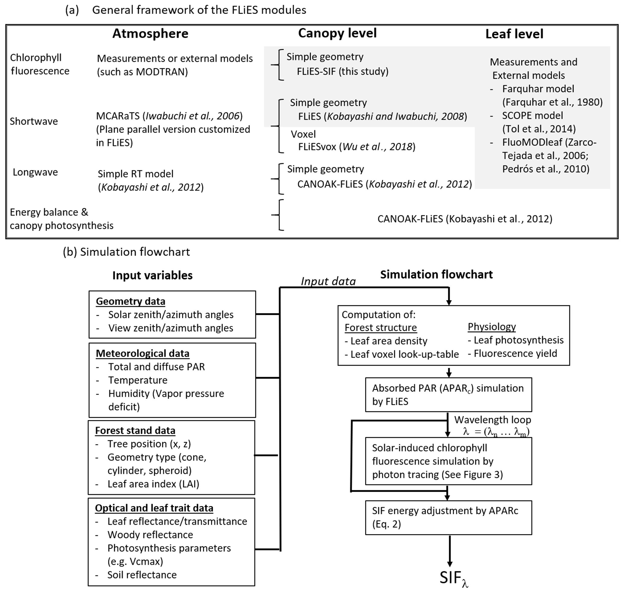
Figure 1General outline of the FLiES modules and simulation flows. (a) General framework of the FLiES modules. Newly developed module in the current study is indicated by the grey-colored background. (b) Simulation flow and input data sets. Four major input data – geometry data, meteorological data, forest stand data, and optical and leaf trait data – are required to run the model.
2.1 General outline of FLiES-SIF
2.1.1 Overall frameworks
We developed a 3-D plant canopy radiative transfer model for simulating the canopy-scale directional SIF radiance (FLiES-SIF version 1.0; Kobayashi and Sakai, 2019). Figure 1a shows the overall framework of the FLiES family modules. The aim of FLiES is to consider the impact of landscape heterogeneity on the radiative processes and determine how this links to the canopy energy, water, and carbon exchange. One of the important aspects of modeling is to make the modules as computationally efficient as possible: most of the FLiES modules, including the newly proposed FLiES-SIF, can be easily run on moderate-level personal computers with relatively modest memory demands and public software (GNU gfortran, gcc, and R). The model development was initiated using 3-D radiative transfer modeling in the shortwave domains (Kobayashi and Iwabuchi, 2008). A 1-D version of the atmospheric radiative transfer model, MCARaTS (Iwabuchi, 2006), was incorporated to simulate the atmosphere–forest radiation interaction. A longwave radiative transfer module was then added, together with energy balance and plant physiology modules (Fig. 1a; Kobayashi et al., 2012; Baldocchi and Harley, 1995). All these modules are related to the radiation emitted in the Stefan–Boltzmann law of the Sun, by the Earth's surface, and by atmospheric media.
The current FLiES-SIF work adds a radiation interaction module for the induced radiation emitted from leaf pigments, and describes how to combine the forest structure information and leaf physiology models (van der Tol et al., 2014; Farquhar et al., 1980) with the fluorescence radiative transfer module (Fig. 1a). The FLiES-SIF model shares some key aspects of numerical schemes in FLiES: it employs a spatially explicit forest landscape (Sect. 2.1.2) and is based on a Monte Carlo ray-tracing approach (Sect. 2.2–2.3). Analogous to the modeling in previous FLiES modules, FLiES-SIF employs a Monte Carlo sampling scheme, where photon-tracing sequences represent the integration form of the radiative transfer equation, or the so-called Neumann series (Antyufeev and Marshak, 1990). In such modeling, the photon path lengths and scattered directions are determined by random numbers and probability distribution functions such as the Lambert–Beer exponential function and the scattering phase function. The scattering and re-absorption of emitted fluorescence light must also be considered to identify the relationship between the fluorescence emitted by the chloroplasts and the top-of-canopy outgoing fluorescence radiance (Porcar-Castell et al., 2014). Several recent studies have worked on the quantification of the impact and modeling of scattering and absorption effects from the leaf scale (e.g., Agati et al., 1993; van der Tol et al., 2019) to the canopy scale (e.g., Romero et al., 2018). Multiple scatterings and re-absorption among leaves, trunks, and soil background can be numerically simulated using unbiased and efficient approaches (Kobayashi and Iwabuchi, 2008). The performance and reliability of FLiES for simulating light transmittance through a canopy and bidirectional reflectance factors have been extensively investigated in previous studies (Widlowski et al., 2011, 2013, 2015). As a default setting, FLiES-SIF version 1.0 simulates the bidirectional SIF radiance at the top of the canopy, but the simulation codes can easily be extended to simulate SIF at any height level within the plant canopy and for the spatial mapping of SIF radiance at the top of the canopy.
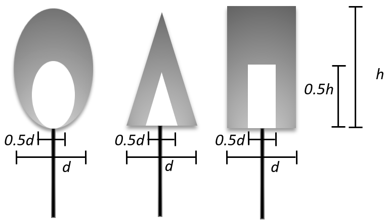
Figure 2Representation of the individual crowns and stems. The tree crown objects are defined as either cone, cylinder, or spheroid, where d is the maximum diameter of the object and h is a crown height. The crown objects are divided by two domains. Outer domains (grey-colored domains in the figure) are filled with green leaves. Inner domains are filled with woody materials. In the default setting, the sizes of inner domains are set as half of the crown size.
2.1.2 Canopy structure represented by FLiES-SIF
The forest landscapes employed in FLiES-SIF consist of simple geometric objects such as cones, spheroids, and cylinders, as in other 3-D models (e.g., DART and FluorFLIGHT) (Fig. 2). The volume domains inside the crown objects can be further split into multiple domains to realize the spatial distribution of the leaf area and woody area densities. This approach is useful in some aspects because (1) it can establish realistic plant canopies in which the majority of leaves are distributed in the outer and upper parts of the crowns (see Fig. 2), and (2) this approach is simple and computationally efficient. The insides of the crown volumes are assumed to be turbid media, where the light attenuation follows the Lambert–Beer exponential law as a function of leaf/woody area densities and leaf inclination angles. The conventional turbid medium approach assumes that the leaves are randomly distributed in space. In the FLiES modules, including FLiES-SIF, a spatially anisotropic arrangement of leaves (the so-called clumping effect) is modeled using re-collision probability theory (Smolander and Stenberg, 2003, 2005; Kobayashi et al., 2010), which is particularly important for the shoot-scale clumping of needleleaf. More details can be found in the FLiES user manual (Kobayashi, 2019). Note that FLiES has a module for the voxel representation of the forest landscape (Wu et al., 2018), but this module is not currently incorporated into FLiES-SIF version 1.0.
The realization of individual tree objects has some degree of freedom in the characterization of leaf and woody densities in crowns. In the sensitivity analysis described in the next chapter, we consider the following forest architectures. The crown objects are separated into two domains, namely the outer leafy-crown and inner woody domains; the outer and inner domains are filled with 100 % leaves and 100 % wood, respectively. The height and diameter of the inner woody domain is set to be half that of the outer domain (Fig. 2). Stems are represented by solid cylinders. The individual tree dimensions can be defined differently. The landscape size used in this study is 100 m×100 m. To create the virtual forest canopy for SIF simulations, it is necessary to determine all of the tree positions in the forest. If ground-based tree census data exist, they can be used to create the virtual forest canopy. The virtual forest canopies can also be reconstructed using a statistical approach (Yang et al., 2018). Assuming that the spatial arrangement of the trees follows a Poisson or Neyman distribution, the individual tree positions are determined by these statistical functions and random numbers.
2.1.3 Simulation flow
The simulation flow of the spectral SIF calculation is shown in Fig. 1b. The FLiES-SIF model requires four major inputs, namely geometry data, meteorological data, forest stand data, and optical data for leaves and other elements (e.g., soil background). The geometry data specify the Sun and sensor view directions (zenith and azimuth angles). The meteorological data are used in the pre-computation of fluorescence yield. The incident total and diffuse photosynthetically active radiation (PAR) data from the top of forest canopies are also used in the canopy radiative transfer module. If no PAR observations are available, these data can be calculated by the FLiES atmosphere module (1-D MCARaTS; see Fig. 1a).
Before running the Monte Carlo ray-tracing processes in the forest canopy, the forest structures (leaf area density and leaf voxel look-up table) and leaf-level physiology (fluorescence module) are computed. In FLiES-SIF, landscape-scale LAI is an input variable. The model requires the leaf area density of individual canopy volumes. FLiES-SIF computes the leaf area density from a given forest landscape and LAI data. Fluorescence ray tracing also requires information about the leaf-level Sun-induced fluorescence yield and its spectral composition. This information is computed by the leaf photosynthesis and fluorescence module. These modules are described in the following subsections (Sect. 2.1.4 and 2.1.5).
Once the forest structure and leaf fluorescence yield have been computed, Monte Carlo ray tracing is performed in the broad PAR domain to determine the PAR absorbed in the forest landscape (APARc in Sect. 2.2). The SIF radiance is then simulated on an individual wavelength basis. Details of the radiative transfer formulation and ray-tracing algorithm are summarized in the following sections (Sect. 2.2–2.5).

Figure 3Voxel extraction from geometric canopy landscapes. The leaf voxel is extracted before the ray-tracing simulation. FLiES-SIF model uses the geometric object approach for the Monte Carlo ray tracing. For the SIF simulation, the ray tracing is initiated from the randomly selected positions in the forest landscape. This voxel information is used to efficiently select the leaf position where SIF occurs.
2.1.4 Creation of the leafy-canopy voxel look-up table
In FLiES-SIF, 3-D forest landscapes are reconstructed using the geometric tree objects described in Sect. 2.1.2 and Fig. 3-upper). The photon tracing starts from an arbitrary position within the leafy-canopy volume. This position is determined by three random numbers corresponding to x, y, and z. When the canopy landscape is sparse, the majority of randomly determined positions v0 will be outside of the leafy-canopy space, which means a large number of trial runs will be required to determine an appropriate position v0. To reduce the computation time, regularly placed leafy-canopy voxel tables are extracted to determine where to start the SIF emission and subsequent photon tracing (Fig. 3). In FLiES-SIF version 1.0, the leafy-canopy voxel information is saved in a look-up table (Fig. 3). The voxel information in the table contains lower and upper corner positions (x, y, z, and x+dx, y+dy, z+dz), the leaf area density (LAD) of the voxel, and the sunlit leaf area density (LADsun). The size of each voxel is currently 1 m3. Note that the extracted leafy voxels are not always completely filled with canopy geometry; canopy edge voxels only partially contain the leafy-canopy geometry. In addition, tree canopy geometries contain branch domains. Thus, even if the voxel is completely inside the canopy geometry, there may be some domains that do not contain leaves.
2.1.5 Computation of leaf-level fluorescence yield
In FLiES-SIF version 1.0, the leaf-level Sun-induced fluorescence yield (hereafter SIF yield; ϕf) is pre-computed and stored in a look-up table prior to ray tracing. The SIF yield ϕf is computed by the model of van der Tol et al. (2014) and Farquhar's photosynthesis model (Farquhar et al., 1980) under various environmental conditions, including APAR. The actual photosynthesis can not be determined without stomata models (e.g., Collatz et al., 1991). The leaf temperature is also dependent on photosynthesis and stomata regulations. These interrelations are solved by iterating the energy balance, stomata, and photosynthesis equations. The CANOAK-FLiES module (Fig. 1a, Kobayashi et al., 2012) can handle such leaf-level coupled physiology phenomena, but this would require more input variables and increase the computational load. Thus, in the current version of FLiES-SIF, we adapted the following assumptions to obtain reasonable photosynthesis simulation results. First, the leaf temperature was assumed to be the same as the surface air temperature. This is usually acceptable, except in very dry conditions when the stomata are almost closed in daytime. The other assumption concerns the stomata modeling. The FLiES-SIF module does not explicitly use the stomata model. Rather, the consequences of the stomata activity, i.e., the downregulation of the intercellular partial CO2 pressure (ipCO2), were modeled as a function of the vapor pressure deficit (VPD). We used the experimental relationships measured by Dang et al. (1997), who investigated the relationships between ipCO2 and VPD in three tree species (pine, spruce, and aspen; see Fig. 10 of Dang et al., 1997). If we simulate SIF over such species, the regression lines given by Dang et al. (1997) can be used. For other species, we created a simplified function based on the relationship derived by Dang et al. (1997):
where apCO2 denotes the ambient partial CO2 pressure.
To simulate the spectral SIF, the spectral composition of SIF must be known. Our approach is similar to that used in the SCOPE model (van der Tol et al., 2009). We derived the spectral composition from the FluorMODleaf model (Zarco-Tejada et al., 2006; Pedrós et al., 2010). The calculated leaf-level spectral SIF radiance variations given by FluorMODleaf were normalized to determine the fraction of SIF at wavelength λ, fs (), with respect to the broadband SIF (W m−2). The standard setting and variables are described in Sect. 3.1. That is, we only used the fraction of spectral composition from the FluorMODleaf model. The radiance was then determined from APAR and ϕf, which varies with environmental conditions and leaf traits such as the maximum carboxylation capacity, Vcmax, used in the photosynthesis model.
2.2 Bidirectional SIF radiance
The bidirectional SIF radiance at wavelength λ at the top of canopy, I(λ,ΩV), can be decomposed into four different light transfer pathways:
where the subscripts “dir” and “ms” indicate the direct emission of SIF and SIF after multiple scatterings, respectively. The direction vector contains the observation zenith and azimuth angles. The radiance elements Idir_sun, Idir_shade, Ims_sun, and Ims_shade on the right-hand side of Eq. (2) indicate direct SIF radiance from sunlit leaves, direct SIF radiance from shaded leaves, sunlit SIF radiance after multiple scatterings, and shaded SIF radiance after multiple scatterings, respectively. Here, the direct emission of SIF indicates SIF that is emitted from leaves and directly escapes from the canopy space without hitting other leaves and trunks. On the contrary, “multiple scattering SIF” indicates SIF that is emitted from leaves, hits other leaves, trunks, or soil background, and then escapes from the canopy space in the view direction. Note that most of the optical and radiance quantities described below are spectral variables. For simplicity of the mathematical expressions, if not explicitly mentioned, the wavelength λ is omitted from subsequent equations.
The intensity of SIF is related to the APAR taken in by the forest canopy. If the forest is sparse or the leaf area density in the tree crowns is low, a large portion of incident PAR is transmitted through plant canopies. The transmitted PAR does not contribute to the SIF emissions on the leaf surface. Thus, if photon tracing is performed under sparsely vegetated canopies, the simulation includes large amounts of photons that are not used to compute SIF. To make the numerical simulation more efficient, we propose a variance reduction technique. FLiES-SIF forces all incident PAR to be absorbed by sunlit or shaded leaves and initiates the photon tracing for SIF emitted from leaves. This procedure artificially enhances or diminishes APAR, biasing the simulated SIF depending on the ratio of actual APAR to the “apparent APAR” (APARapp) used in the simulation. Thus, the simulated SIF under the APARapp is adjusted to the actual APAR (APARc) conditions:
where I(ΩV) and I′(ΩV) denote the SIF radiance with APARc and APARapp, respectively. APARapp is simulated with the SIF simultaneously. The APARc is independently calculated for a given canopy landscape before the SIF simulation (Fig. 1b and Sect. 2.1.3). In subsequent sections, we describe the radiance components derived with APARapp (, , , and ).
2.3 Calculation of direct SIF radiance
The direct SIF radiance from sunlit and shaded leaves is calculated by summing all direct SIF radiation contribution factors of the ith photon (ψdir,i):
where Vsun, Vshade, v0, and N indicate the classes of sunlit and shaded leaves, the position of the photon , and the total number of photons, respectively.
The direct SIF radiation contribution factor of the ith photon ψdir, i can be decomposed into three components: leaf-level SIF emission weight w0, directional emission transfer function (the so-called phase function Pf), and attenuation function:
Here, τV is the optical thickness of the plant canopy in the view direction ΩV. The factor 2π is a normalization factor for the phase function Pf. These three components in ψdir, namely w0, Pf, and exp (−τV), indicate the SIF emitted in all directions from both adaxial and abaxial sides of a single leaf, the fraction of SIF emitted in the view direction, and the fraction of SIF attenuation to the top of the canopy in the view direction, respectively.
2.3.1 Attenuation function
The attenuation of SIF in the view direction Ωσ is calculated by the attenuation function exp (−τV). When the hotspot effect is not considered, the attenuation function is expressed using the plant canopy gap fraction theory:
where ui, si, Gσ,i, and γi are the leaf area density, path length, mean leaf projection area, and clumping index of the ith tree. They are aggregated over the trees located in the light path between the emission point to the top of canopy in the view direction, respectively. The path length, s, is a sum of canopy paths that penetrates through crown objects.
The mean leaf projection area G is a function of the leaf inclination angle distribution function gL and an arbitrary direction Ωσ (such as the Sun direction ΩS or view direction ΩV):
Generally, the clumping index contains various nonrandom scales of spatial leaf distributions, from the shoot to the landscape scale. Because FLiES-SIF version 1.0 employs explicit tree crown landscapes, clumping larger than the crown scale need not be considered. However, the crown volumes are expressed as turbid media: if the leaves are not randomly distributed in the crown object, e.g., shoot-scale clumping (Cescatti and Zorer, 2003; Chen et al., 1997), attenuation must be corrected according to the shoot-scale clumping index. In FLiES-SIF version 1.0, the shoot-scale clumping index is estimated by the spherically averaged shoot silhouette area (Cescatti and Zorer, 2003). Details on how shoot-scale clumping is incorporated can be found in a previous report (Kobayashi et al., 2010). The hotspot effect refers to the strong illumination near the solar direction (). When the hotspot effect is non-negligible, the modified optical thickness τ′ is expressed as
where H is a hotspot function expressed by the Hapke model (Hapke, 2012), which is used in the framework of the FLiES model (Kobayashi and Iwabuchi, 2008):
where Ωj, l, and αj indicate the incident direction after the jth scattering, the radius of the disk-shaped flat leaves, and the scattering angle (), respectively.
2.3.2 Leaf-level SIF emission weight
The leaf-level SIF emission weight w0 can be calculated from the SIF yield ϕf and APAR on the leaf surface (APARL):
where fs is the fraction of SIF at wavelength λ () with respect to the broadband SIF (W m−2). Thus, fs is a function of wavelength. The SIF yield ϕf is a function of APARL and various environmental and leaf trait variables such as ambient air temperature, humidity, CO2 concentration, and carboxylation capacity (van der Tol et al., 2014). In FLiES-SIF version 1.0, ϕf is read from a look-up table across a wide range of APARL, which should be pre-computed by the leaf-level SIF yield models.
The exact computation of APARL under the angular dependency of PAR can be performed by backward ray tracing at the given position of a leaf, but this approach is time consuming. For more efficient simulations, the values of APARL for sunlit and shaded leaves are approximated as the product of the incident-diffuse PAR and the attenuation function exp (−τs) integrated over the upper hemisphere:
where PARdir and PARdif denote the incident direct and diffuse PAR, respectively, ωPAR is the average single-scattering albedo in the PAR spectral domain (400–700 nm), and ωPAR is the sum of the leaf reflectance rPAR and transmittance tPAR in the PAR domain (). This equation assumes that diffuse PAR is isotropic over the sky and neglects direct PAR scattered within the plant canopy and soil background. Thus, APARL may be underestimated when the background reflectance is high, such as in the case of snow cover. To further reduce the computation time, the hemispherical integration of the attenuation function is approximated by an average of the limited-angle samplings. Details of the computation method are given in Sect. 2.5.
2.3.3 Phase function for SIF emissions
The phase function for SIF emissions Pf gives the fraction of SIF emitted in the view direction ΩV. Similar to the scattering phase function for the reflection of solar illumination, Pf can be determined by the following equations:
where fada and faba are the fraction of SIF emissions from the adaxial and abaxial sides of a leaf; . Note that, in our definition, we have assumed that illumination by solar beams is always on the adaxial side of a leaf.
2.4 Multiple scattering
SIF emissions from the leaf surface occur in all directions (upward and downward in the plant canopy), although they are not always isotropic, as shown in Sect. 2.3.3. A certain portion of SIF does not directly go toward the sky. This portion hits other leaves, trunks, or soil background. The SIF energy from those impacts is scattered, goes in another direction, and then impacts something else. We define this process as the multiple scatterings of SIF. After multiple scatterings, some of the SIF energy will return to the view direction, which enhances the observed SIF radiance depending on the magnitude of the multiple-scattering contribution. The multiple-scattering process of SIF is the same as the scattering process of solar radiation, and the multiple-scattering component can be formulated in exactly the same way as the bidirectional reflectance factor described in Kobayashi and Iwabuchi (2008). The scattered SIF radiance emitted by sunlit and shaded leaves is defined as Ims_sun and Ims_shade, respectively, and these radiance contributions can be calculated by summing all of the scattering contributions:
Here, ψi,j is calculated as follows:
where wi,j is the weight of the ith photon after the jth scattering obtained by using the single-scattering albedo in the SIF spectral domain (). Equation (15) is exactly the same as the multiple scatterings in the shortwave radiative transfer (Kobayashi and Iwabuchi, 2008). The form of the phase function P(Ωj,ΩV) is also described by Eq. (7) in Kobayashi and Iwabuchi (2008). The attenuation function is the same as described in Sect. 2.3.1.
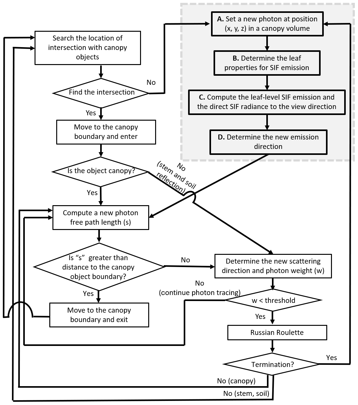
Figure 4The flowchart of the Monte Carlo photon-tracing scheme in canopy landscapes at a single wavelength. Procedures A to E, framed by the dotted grey rectangle, indicate the photon-tracing scheme for direct SIF emission. The other part of the flowchart corresponds to multiple scattering. The multiple scattering schemes are the same as the original FLiES model (Kobayashi and Iwabuchi, 2008).
2.5 Photon-tracing algorithm
The numerical scheme of the photon tracing is shown in Fig. 4. The procedures framed by the dotted grey rectangle indicate the photon-tracing scheme for direct SIF emissions. The area outside the dotted grey rectangle corresponds to scattered photon tracing. The algorithm for scattered photon tracing is exactly the same as the photon-tracing method for solar radiation. Here, we focus on the SIF emission scheme in the grey rectangle. Details of the scattered components are summarized in Kobayashi and Iwabuchi (2008).
2.5.1 Procedure A: set a new photon in the leafy canopy
The position from which SIF emission occurs within a leafy-canopy domain is determined by random numbers. The position v0 is determined as follows. First, an arbitrary voxel is chosen at random from the voxel table (Fig. 3). The exact position () within a selected voxel is then determined by three random numbers (Rx, Ry and Rz; ):
where denotes the position of the lower corner of the selected voxel. If the selected voxel is an edge voxel or contains branch domains, the randomly determined position v0 may be outside the leafy canopy. Therefore, the position v0 is checked to determine whether it is in the leafy domain. If the position is outside the leafy domain, the program generates a new random number and selects another voxel. This procedure continues until the leafy-canopy position v0 is obtained.
2.5.2 Procedure B: determination of the leaf properties for SIF emission
After position v0 has been determined, the leaf properties at the selected position are determined. Two leaf properties are required to continue the computation of the SIF emission: the leaf illumination status (sunlit or shaded) and the leaf surface normal vector . The sunlit leaf area fraction Psun at v0 is computed using the interception of direct sunlight:
where Lp is the cumulative LAI at v0 along the path of the sunlight and GS is a mean leaf projection area defined in Eq. (7). The leaf illumination status (sunlit or shaded) is then determined by a random number R:
The leaf surface normal vector ΩL is also required because the leaf-level SIF emission is related to APAR at the leaf surface (APARL). APARL is computed from the cosine of the sunlight and leaf normal angles. Assuming the leaves are randomly distributed, the azimuthal angle of the leaf surface normal ϕL can be determined by
For a given leaf angle distribution function gL:=g(θL), the zenith angle of the leaf surface normal θL can be determined by the rejection method. In the first step, θL is calculated using a random number:
Then, θL is further evaluated using gL:
If θL is rejected by the abovementioned criteria in Eq. (21), the program returns to Eq. (20) and calculates another θL. In Eq. (21), the evaluation function is a form of leaf angle distribution function multiplied by a sine value. This sine comes from the Jacobian of the polar coordinate and is necessary because gL is defined in polar coordinates.
2.5.3 Procedure C: compute the leaf-level SIF emission and the direct SIF radiance in the view direction
Once the position v0 and leaf properties have been determined, the leaf-level SIF emission w0 and the direct SIF radiance (Idir_sun and Idir_shade) can be computed using the equations derived in Sect. 2.2 and 2.3. The calculation of w0 includes the spherical integration of the attenuation function (Eqs. 11 and 12), which is time consuming. Thus, FLiES-SIF version 1.0 approximates this spherical integration by taking the average of five directions (, (60, 0∘), (60, 90∘), (60, 180∘), and (60, 270∘). We tested the performance of this five-angle assumption by comparing with 10∘ interval samplings (9 zenith and 36 azimuth angles is equal to 324 angle samplings). When the attenuation functions were computed by these two angle samplings at 104 randomly selected positions in the forest landscapes used in the sensitivity analysis in Sect. 3, the mean absolute error of this approximation was 14.6 % (N=10 000). Finally, Idir_sun and Idir_shade are calculated by the local estimation method using Eqs. () and (5) (Antyufeev and Marshak, 1990; Marchuk et al., 1980).
2.5.4 Procedure D: determination of the new emission direction
Direct SIF radiance in the view direction ΩV is determined by procedure C. The multiple scattering contribution is further evaluated by photon tracing. To start the photon tracing, the emission direction Ω(θ, ϕ) is calculated using two random numbers and the leaf surface normal vector . Assuming that the SIF emission is bi-Lambertian on the leaf surface, the zenith and azimuthal angles relative to the leaf normal (α, β) are determined by
The scattering direction Ω(θ, ϕ) in the Cartesian coordinate system is then calculated by a coordinate transformation from (α, β) to (θ, ϕ).

Figure 5The forest landscape used in the sensitivity analysis. The landscape size is 1 ha (100 m×100 m). The tree positions and canopy heights are determined by the random numbers. (a) Default forest: crown shape is spheroid, tree density is 359 trees ha−1, canopy layer height is 5–20 m, and crown coverage is 88 %. (b) Tropical broadleaf forest: crown shape is spheroid, tree density is 1816 trees ha−1, canopy layer height is 5–30 m, and crown coverage is 88 %. (c) Evergreen needle forest: crown shape is cone, tree density is 3592 trees ha−1, canopy layer height is 5–15 m, and crown coverage is 49 %. (d) Savanna: crown shape is spheroid, tree density is 96 trees ha−1, canopy layer height is 5–10 m, and crown coverage is 19 %.
We created a 1 ha virtual forest as a default conditions (Fig. 5a). Test simulations of the SIF emissions were performed to evaluate the FLiES-SIF model performance and understand the sensitivity of SIF against various input variables including forest structures. We evaluated the model by four step exercises. First, we conducted the intercomparisons with the existing 3-D model (Discrete Anisotropic Radiative Transfer; DART) to quantify the inter-model differences (Sect. 3.2). Secondly, we performed the sensitivity analysis against geometric conditions (solar zenith angle, SZA; view zenith angle, VZA), sunlit leaf fraction, and LAI, and to identify the factors (hotspots, light attenuation, phase function, weight of photons) that contribute to SIF radiance under the given forest structure (Sect. 3.3). Thirdly, we ran the FLiES-SIF model with different forest landscapes to show how the 3-D forest structures such as crown shape, tree size, and crown cover influence the simulated SIF (Sect. 3.4). Fourthly, we performed 1-D and 3-D comparisons in an actual diurnal variations in total and diffuse PAR observed in Yokohama, Japan (35∘22′ N, 139∘37′ E), in the summer of 2014 (Delta-T sunshine sensor, Delta-T Co. Ltd.) (Sect. 3.5). In this exercise, we evaluated the potential errors (overestimation) in the 1-D homogeneous layer (turbid medium) approach. We compared in seven different scenarios that include different leaf angle distributions (spherical, erectrophile, and planophile) and within-crown clumping (γ=0.6) in the 3-D landscapes (Table 1). Lastly, we evaluated the sensitivity of the leaf-level fluorescence yield (Sect. 3.6). In this exercise, we computed the leaf-level fluorescence with the FLiES-SIF physiology module (Fig. 1b).
Table 1Simulation scenarios for the 1-D and 3-D comparisons with an actual diurnal incident PAR data.
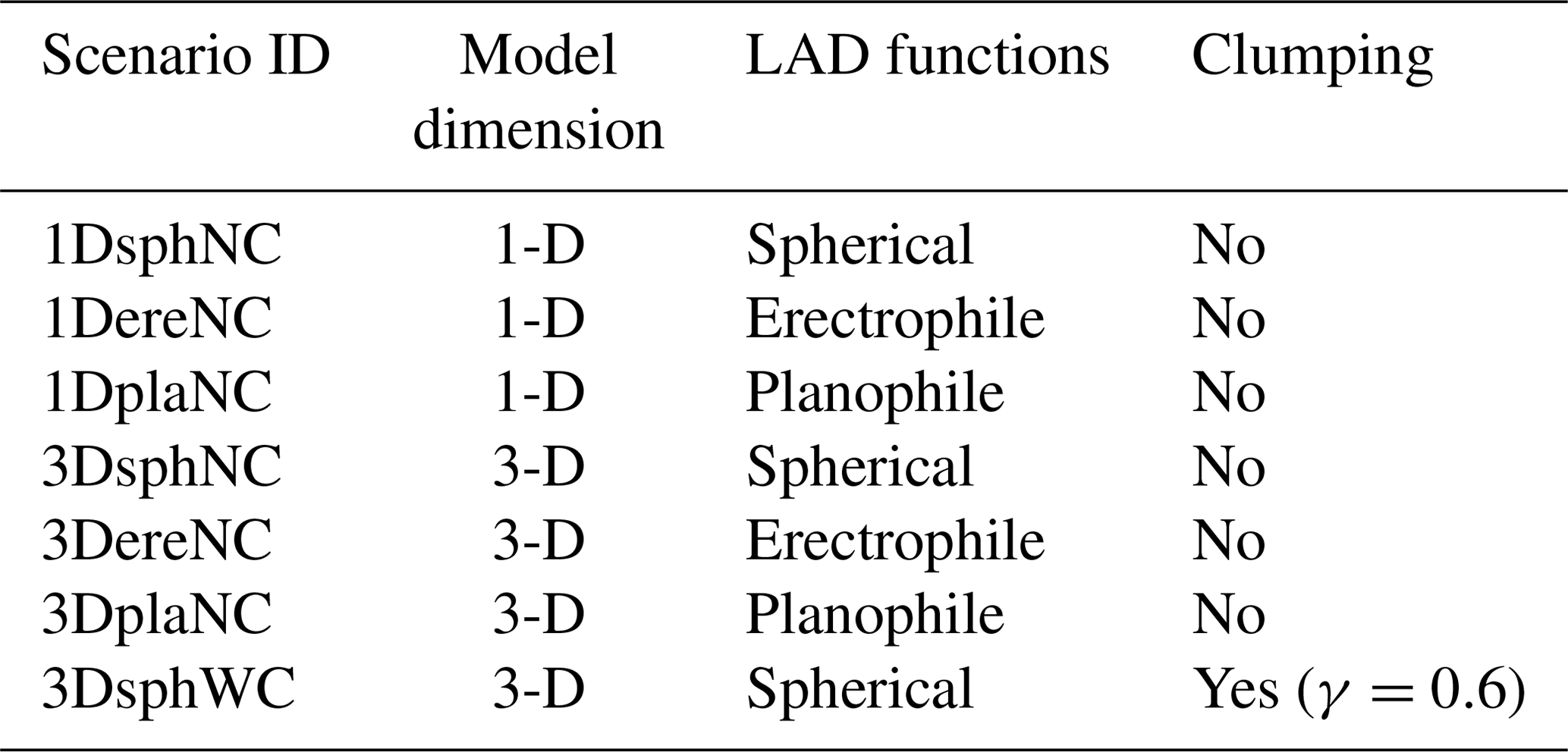
LAD is leaf angle distribution.
Table 2Optical data in PAR domain used in the sensitivity analysis.
3.1 Input data and simulation condition
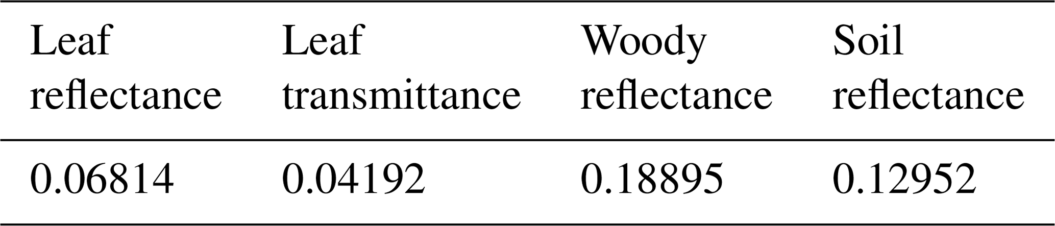
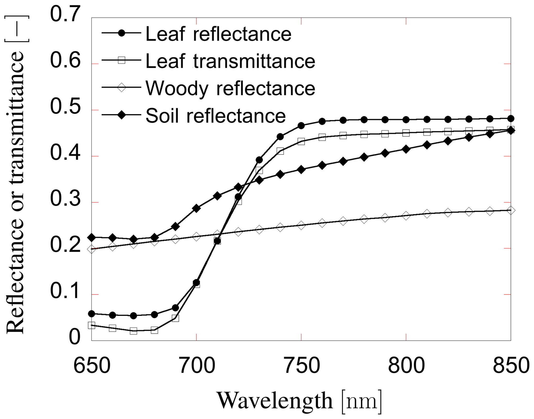
The individual tree positions and sizes were determined at random. The spheroid shape was employed for the individual crowns. The tree density used in the sensitivity analysis was 359 trees ha−1. The canopy layer height was set to 25 m (Fig. 5) and the crown coverage was 96 %. FLiES-SIF assumes that all crowns have the same leaf area density. The spherical leaf angle distribution function was used. We also used three different landscape conditions – tropical broadleaf (Fig. 5b), evergreen needleleaf (Fig. 5c), and savanna (Fig. 5d) – to understand the effect of landscape structure on SIF. The model requires optical data in the PAR domain and the spectral wavelength to be simulated. In this sensitivity analysis, we used the data assembled by Kobayashi (2015a). Figure 6 shows the spectral leaf reflectance and transmittance and the woody/soil reflectance. The leaf reflectance and transmittance, woody reflectance, and soil reflectance were calculated from various broadleaf spectral data, medium reflective woody elements, and medium reflective soil surfaces in Kobayashi (2015b), respectively. All optical data were averaged over 10 nm intervals between 650 and 850 nm. The optical data in the PAR domain were computed as the average from 400 to 700 nm (Table 2). The same woody reflectance data were used for both stem surface and branch materials. The fractions of SIF emission (fada, faba) were determined using the FluorMODleaf model (FluorMODgui V3.1) (Zarco-Tejada et al., 2006; Pedrós et al., 2010) (Fig. 7). To run FluorMODgui V3.1, we used the default biochemical parameters (leaf structure parameter N=1.5, chlorophyll a+b content Cab=33.0 µg cm−1, water content Cw=0.025 cm, dry matter content Cm=0.01 g cm−2, fluorescence quantum efficiency Fi=0.01, leaf temperature T=20.0 ∘C, species temperature dependence = 2 (beans), stoichiometry of PSII (photosystem II) to PSI reaction centers S to=2.0) under the downward spectral sky radiation data (direct transmittance in Sun direction (τS), FluorMOD30V23.MEP). The fractions of SIF emission were derived from the simulated leaf fluorescence output by normalizing the simulated leaf-level SIF from the adaxial and abaxial sides. In this sensitivity analysis, we employed two types of leaf-level SIF yield ϕf. The first type is a constant value of 0.01 throughout the whole APAR range from Sect. 3.2 to 3.5. This value is used to test the impact of forest structures (LAI) and Sun and observation geometries on SIF. The second type is an APAR-dependent value derived using the models of van der Tol et al. (2014) (Fig. 8) and Farquhar et al. (1980). Tol's model is based on energy partition within leaves in Sect. 3.6. In calculating ϕf, we used the leaf fluorescence and physiology module in the FLiES-SIF model as described in Sect. 2.1. The parameter values in these models were set by reference to previous literature (such as van der Tol et al., 2014; De Pury and Farquhar, 1997), and the results compared with those using a constant APAR-dependent (Tol's model) ϕf. In the test simulation except Sect. 3.5, the incident total PAR on the canopy surface was fixed at 2000 , except for in the APAR sensitivity analysis, and the fraction of diffuse radiation was fixed at 0.3. In the sensitivity analysis, we used 105–106 photons in each model run. Figure 9 indicates the dependency of SZA and LAI on total SIF radiance between 650 and 850 nm. In the following section, we analyze the SIF sensitivity in λ=760 nm.
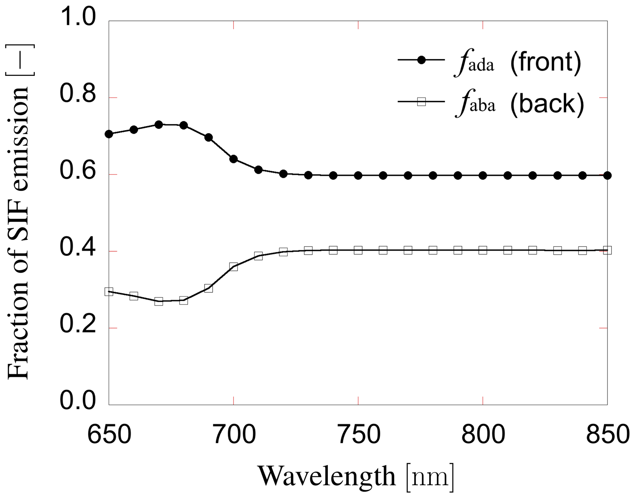
Figure 7The fraction of SIF emission from adaxial and abaxial side of leaves. This ratio was determined by the leaf-level chlorophyll fluorescence model (the FluorMODleaf model (FluorMODgui V3.1) (Zarco-Tejada et al., 2006; Pedrós et al., 2010).
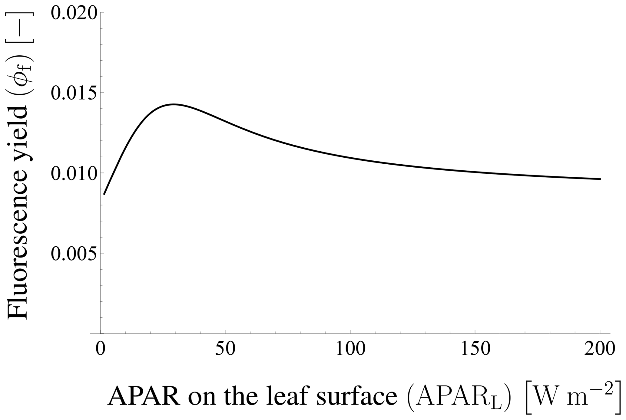
Figure 8Fluorescence yield in Tol's model. The fluorescence yield depends on APAR on the leaf surface. In this case, ϕf is almost unchanged when APARL is greater than 200 W m−2.
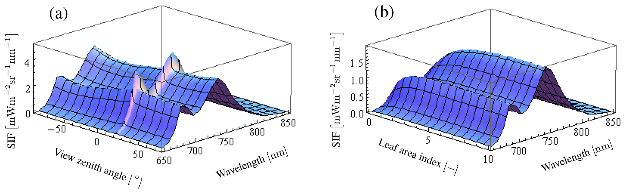
Figure 9Variation of SIF radiance depending on VZA and LAI in the wavelength of 650 to 850 nm. Panel (a) indicates VZA dependence of SIF at LAI of 3.0 and SZA of 20∘. There is a strong peak in the Sun direction at the whole wavelength. Panel (b) indicates LAI dependence of SIF at VZA of 0∘ and SZA of 20∘. SIF radiance increases with LAI and then becomes saturated.
3.2 Intercomparisons with the DART model
To demonstrate the efficacy of FLiES-SIF for calculating the SIF radiation, we compared the output with that of DART (Gastellu-Etchegorry et al., 2017), which is one of the available 3-D models. We adopted the flux-tracking mode in the radiative method of DART version 5.7.6 to calculate the SIF radiation and compared the simulation results under the following conditions: SZA=30∘, SAA (solar azimuth angle) = 0∘, and λ=760 nm. Only part of the default landscape (40 m×40 m, 50 trees) was simulated to reduce the computational load. Figure 10 compares the SIF radiation calculated by FLiES-SIF with that given by DART-SIF. In terms of VZA dependency, FLiES-SIF overestimates SIF radiation by about 18 % on average in the forward direction (VZA>0), and the difference becomes larger as VZA increases. In contrast, FLiES-SIF underestimates the SIF radiation by about 12 % in the backward direction (VZA<0), and the difference reaches a maximum at ∘. In terms of LAI dependency, FLiES-SIF overestimates SIF radiation by about 9 % on average, with the difference being especially pronounced when LAI>6. The SIF radiation increases with LAI in FLiES-SIF but decreases as LAI increases in the DART model. As a result, FLiES-SIF gives similar SIF radiation values to those given by DART and has greater sensitivity to angles.
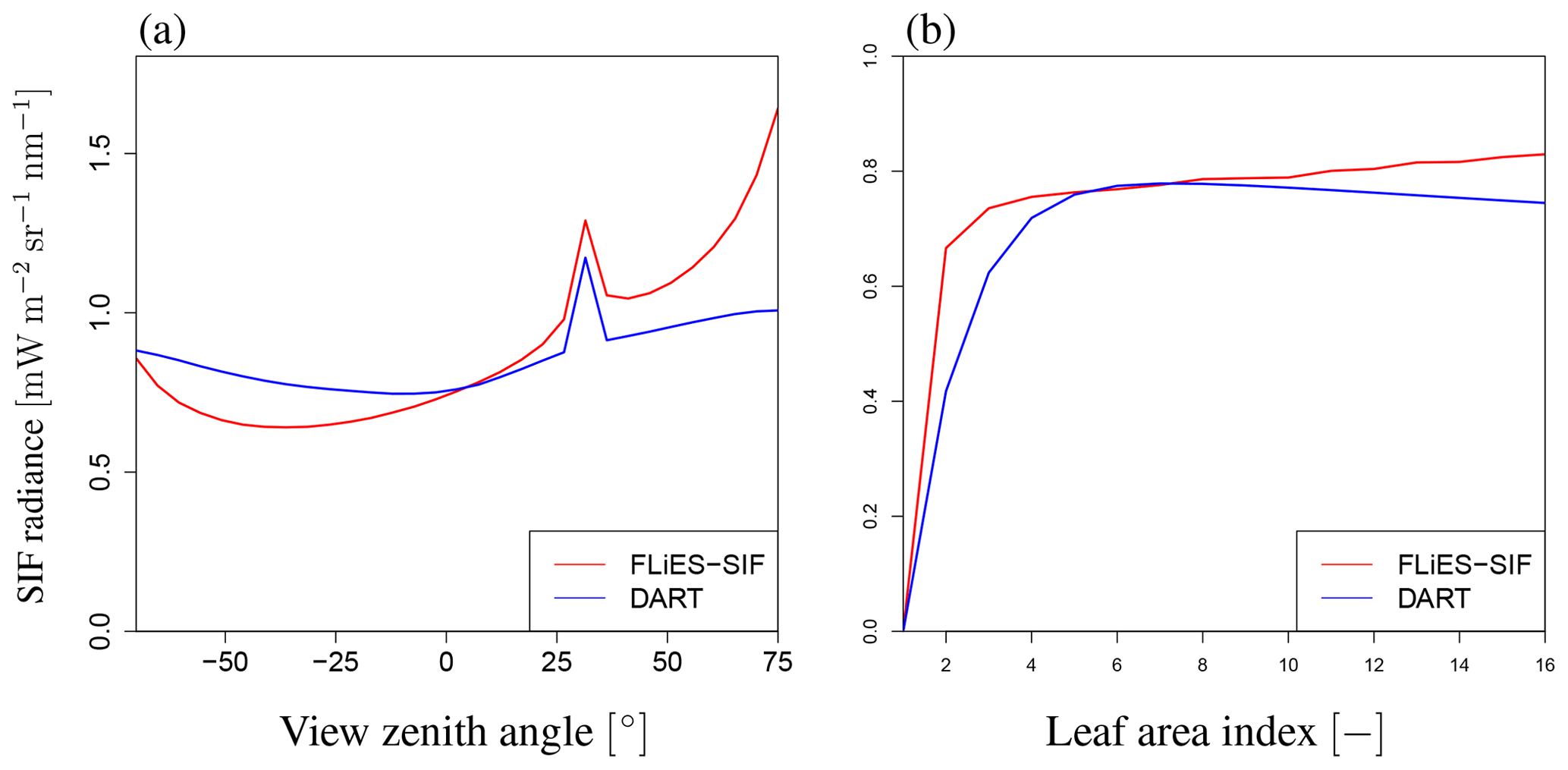
Figure 10Comparison of SIF radiance with DART model. These figures indicate (a) VZA dependency (LAI of 3.0) and (b) LAI dependency (VZA of 0∘), respectively. SZA and SAA values are 20 and 0∘, respectively. The red and blue lines indicate the results of FLiES-SIF and DART, respectively. FLiES-SIF has similar dependency on LAI and VZA to DART, although FLiES-SIF has higher angular dependency.
FLiES-SIF is a reasonable and proper model for determining the SIF radiation. The DART model has a useful graphical user interface (GUI) and can calculate SIF radiation on complex landscape structures using many kinds of 3-D objects. However, unlike FLiES-SIF, DART does not include a leaf physiological module. Additionally, FLiES-SIF requires less computational resources than the DART model.
3.3 Sensitivity analysis with default forest landscape
3.3.1 Angular dependency of SIF
Figure 9a shows the total SIF radiance for wavelengths between 650 and 850 nm. These figures indicate that the SIF radiance shows a strong peak near the Sun direction over the whole wavelength range, although the SZA value, which exhibits the maximum SIF, varies according to the wavelength. In the visible red region, the SIF radiance reaches an extremum at a lower SZA than in the near-infrared region. Regardless of wavelength, the angular dependency of SIF exhibits similar patterns: in the direction of forward emission (VZA>0), SIF increases with an increase in VZA and sharp strong peaks appear around the Sun direction (the hotspot effect). In the backward direction (VZA<0), the SIF decreases with an increase in |VZA| and attains a minimum at around −35 to −50∘, before increasing with |VZA|. Although the general angular patterns are similar across the whole wavelength range, the strength of the hotspot peak in the forward direction and the minimum SIF in the backward direction vary slightly with the wavelength.
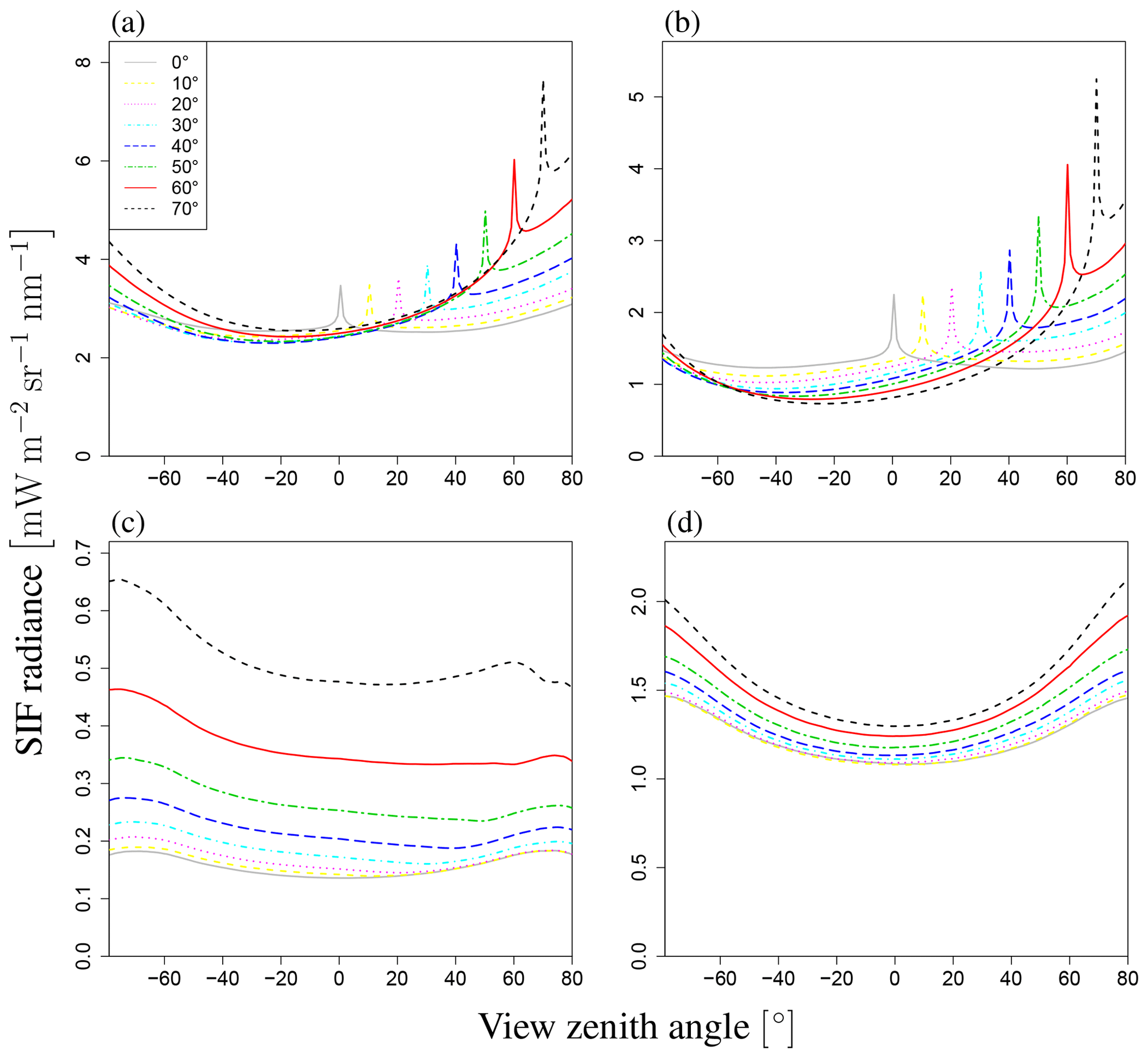
Figure 11Angular dependence of SIF. This figure shows total radiance I (a), direct radiance from sunlit leaves Idir_sun (b), direct radiance from shaded leaves Idir_shade (c), and radiance after multiple scatterings Ims_sun+Ims_shade (d) at LAI of 3.0. Each line represents a different SZA (0–70∘). Negative values of SZA represent the backward direction, and positive values represent the forward direction on the principal plane. The angular dependency varies greatly among these radiances.
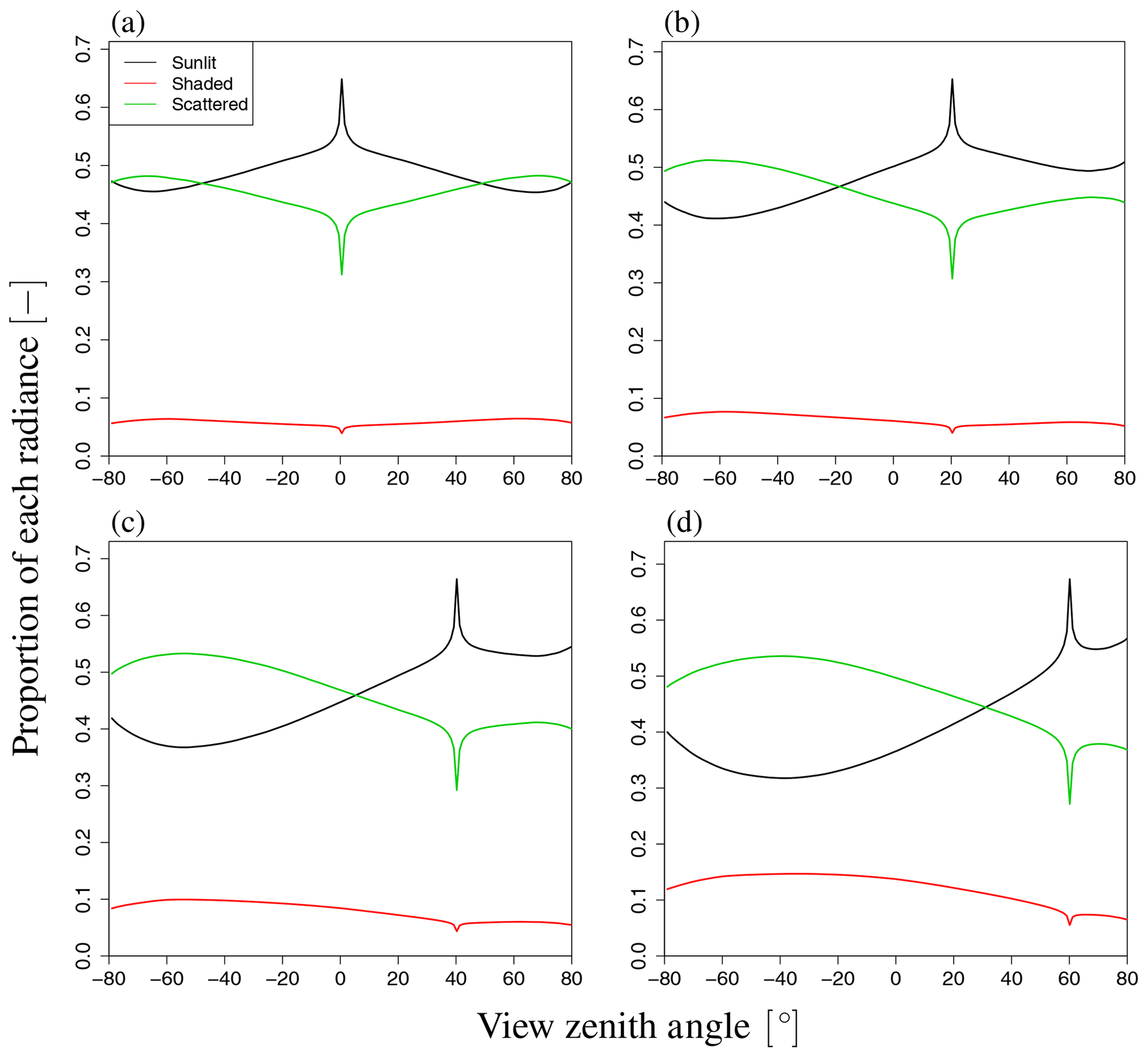
Figure 12Proportion of SIF radiance with respect to VZA variation. Each figure shows the result under a different SZA value: (a) 0∘, (b) 20∘, (c) 40∘, and (d) 60∘. The contribution of shaded leaves is basically small, and the contribution rates of the other two radiances exhibit some angular dependency. In the backward direction, the contribution of scattered radiation to SIF is greater than that in the forward direction.
To analyze the dependency of VZA in more detail, we explored the influence of VZA on three terms in Eq. (2), namely the direct SIF from the radiance of sunlit and shaded leaves (Idir_sun, Idir_shade) and the scattered radiance (Ims_sun+Ims_shade), as well as the total SIF radiance (I). The simulated SIF shows distinct angular features for each SIF component (Idir_sun, Idir_shade, Ims_sun+Ims_shade). Figure 11 shows the dependence on VZA of the SIF components when LAI=3.0 for a wavelength of 760 nm. Idir_sun has a strong peak near the Sun direction because of the hotspot effect, whereas angular changes of Idir_sun in other domains are minor. In contrast, Ims_sun+Ims_shade exhibits bowl-like shapes (Fig. 11d), which contributes to the enhancement of total SIF at higher angles. In the FLiES-SIF model framework, SIF radiance is computed by collecting the contribution factor (Eqs. 5 and 15) from the attenuation function, weight of photons, and phase function. Among those factors, the drastic changes in the optical thickness of the attenuation function (Eqs. 6–10) contributed the most to the hotspot in Isun_dir. The attenuation function displays a strong peak around the Sun direction because of the hotspot parameter (H in Eq. 9). When αj is sufficiently large and the hotspot effect is marginal, the attenuation function is determined by the forest structure (such as LAI and leaf angle density). Away from the Sun direction, the SIF radiance gradually decreases or increases slightly. This angular feature (VZA) is influenced by the initial photon weight and phase function through the dependency on the leaf surface normal: the initial photon weight is calculated as the inner product between the leaf angle and the Sun direction. The influence of SZA on the phase function is greater than that on the initial photon weight. The other two components (Idir_shade, Ims_sun+Ims_shade) contribute to the total SIF increase in higher angular domains. In addition, Idir_shade makes a slightly larger contribution in the backward direction, because shaded leaves tend to be more aligned with the backward direction. The shaded leaves only absorb diffuse sky radiation, so the relative magnitude of Idir_shade with respect to Idir_sun greatly depends on the fraction of diffuse radiation. The contributions of these three components in four different Sun angles are presented in Fig. 12. These partitions vary with the fraction of incoming diffuse radiation, optical properties (leaf reflectance and transmittance, woody and soil reflectance), and the leaf area.
3.3.2 Angular dependencies of APAR and sunlit leaves
Because SIF radiance is greatly affected by the APAR of the leaves, the angular behavior of APAR is essential in understanding the numerical computation of SIF emissions. In the FLiES-SIF model, the SIF radiance is first computed under the apparent APAR (APARapp) conditions (Sect. 2.2) and then adjusted by multiplying by the ratio of APARc to APARapp (Eq. 3). The simulated angular patterns indicate that APARc increases with an increase in SZA (Fig. 13b). The increase in APARc with respect to SZA corresponds to the increase in the photon pathlength inside the forest canopy. As SZA increases, more photons are likely to hit leaves before they pass through the canopy layers. In contrast, APARapp decreases as SZA decreases (Fig. 13a). This is because APARapp is related to the fraction of sunlit leaves. As described in simulation procedure C in Sect. 2.5, the photon tracing is initiated from either sunlit or shaded leaves at randomly selected positions. As the LAI along the photon path (Lp) increases, the gap fraction Psun becomes smaller (Eq. 17). As a result, shaded leaves are more likely to be selected in the random process in Eq. (18). In other words, as the fraction of shaded leaves increases, the amount of energy in the simulated system decreases. In the Monte Carlo simulations, the statistical accuracy of the simulated variables depends on the number of photon samplings. The decrease in APARapp does not affect the simulated accuracy of the total SIF radiance; however, it does affect the individual components in Eq. (2), which means the statistical accuracy of Idir_sun decreases as SZA increases. Depending on the target sampling variables to be simulated, the number of photons should be determined (i.e., more photons may be necessary to investigate the behavior of Idir_sun in cases where the sunlit leaf fraction is low).
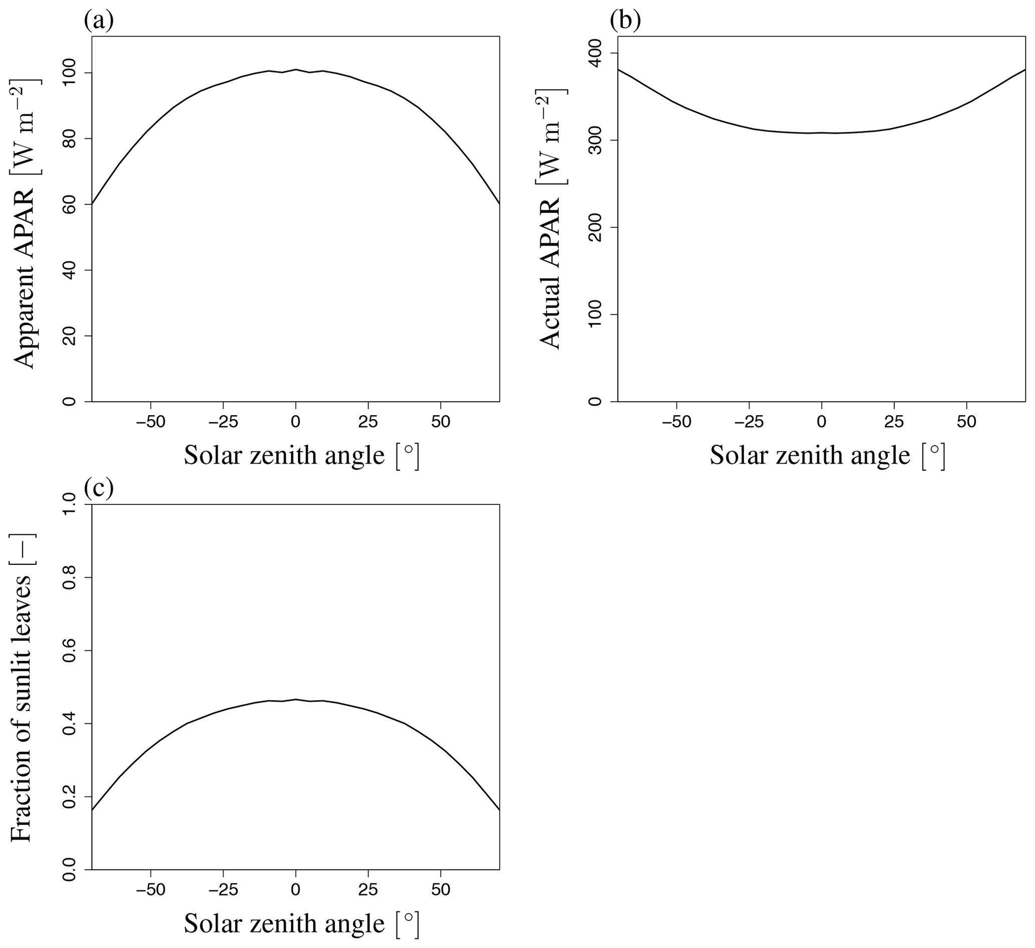
Figure 13Variation of apparent and actual APAR and fraction of sunlit leaves with SZA. (a) Apparent APAR (APARapp), (b) actual APAR (APARc), and (c) fraction of sunlit leaves (Fsun) at LAI of 3.0. These variables are not affected by VZA. APARapp and Fsun decrease and APARc increases with an increase in |SZA|.
3.3.3 Leaf area density dependency
Figure 9b shows the sensitivity of total SIF radiance to LAI for wavelengths of 650–850 nm. The simulated SIF increases with LAI and then becomes saturated over the whole wavelength range, although the speed of saturation varies with the wavelength. In the visible domain, the simulated SIF becomes saturated when LAI=2. In the near-infrared domain, the simulated SIF is not saturated at higher LAI values, indicating that SIF is more sensitive to LAI in the near-infrared domain. To analyze the dependency on LAI, we explored the influence of LAI on three terms in Eq. (2), namely Idir_sun, Idir_shade, and Ims_sun+Ims_shade, as well as the total SIF radiance (I) (forward direction in Fig. 14 and backward direction in Fig. 15). In our simulation scenarios, Idir_sun contributed about 54 % of total SIF radiance when LAI=3, VZA=10∘, and SZA=20∘. Idir_hade and Ims_sun+Ims_shade contributed 7 % and 39 %, respectively (Fig. 16). Figures 14 and 15 show that the individual SIF components respond differently to the LAI.
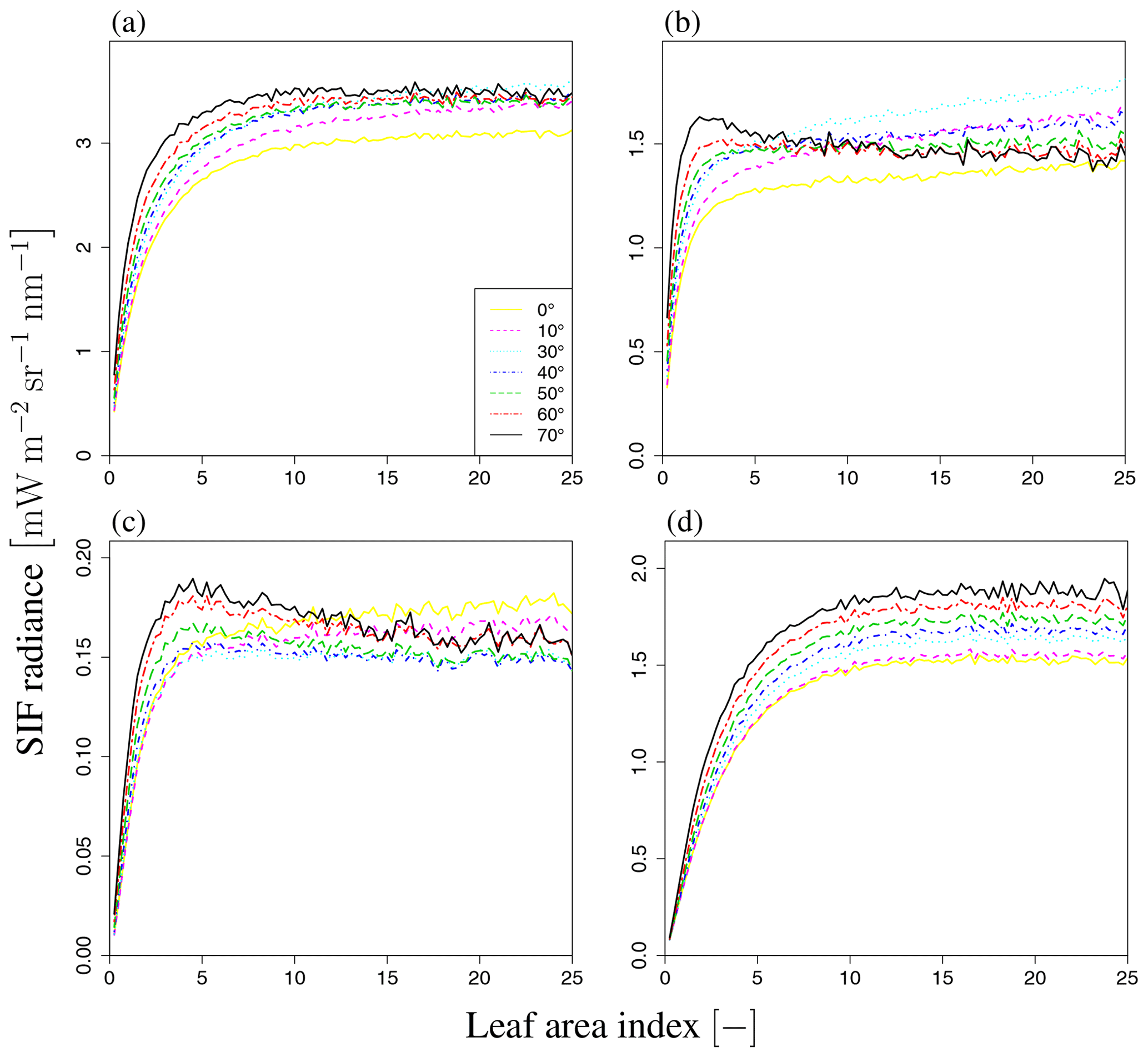
Figure 14LAI dependency on SIF radiance. (a) Total radiance I, (b) direct radiance from sunlit leaves Idir_sun, (c) direct radiance from shaded leaves Idir_shade, and (d) radiance after multiple scatterings Ims_sun+Ims_shade at SZA of 20∘ and SAA of 0∘ (forward direction). Each line represents a different VZA value (0–70∘). SIF radiance increases with LAI and then becomes saturated in most cases. However, when VZA is large (e.g., black and red lines), the direct radiance decreases with an increase in LAI.
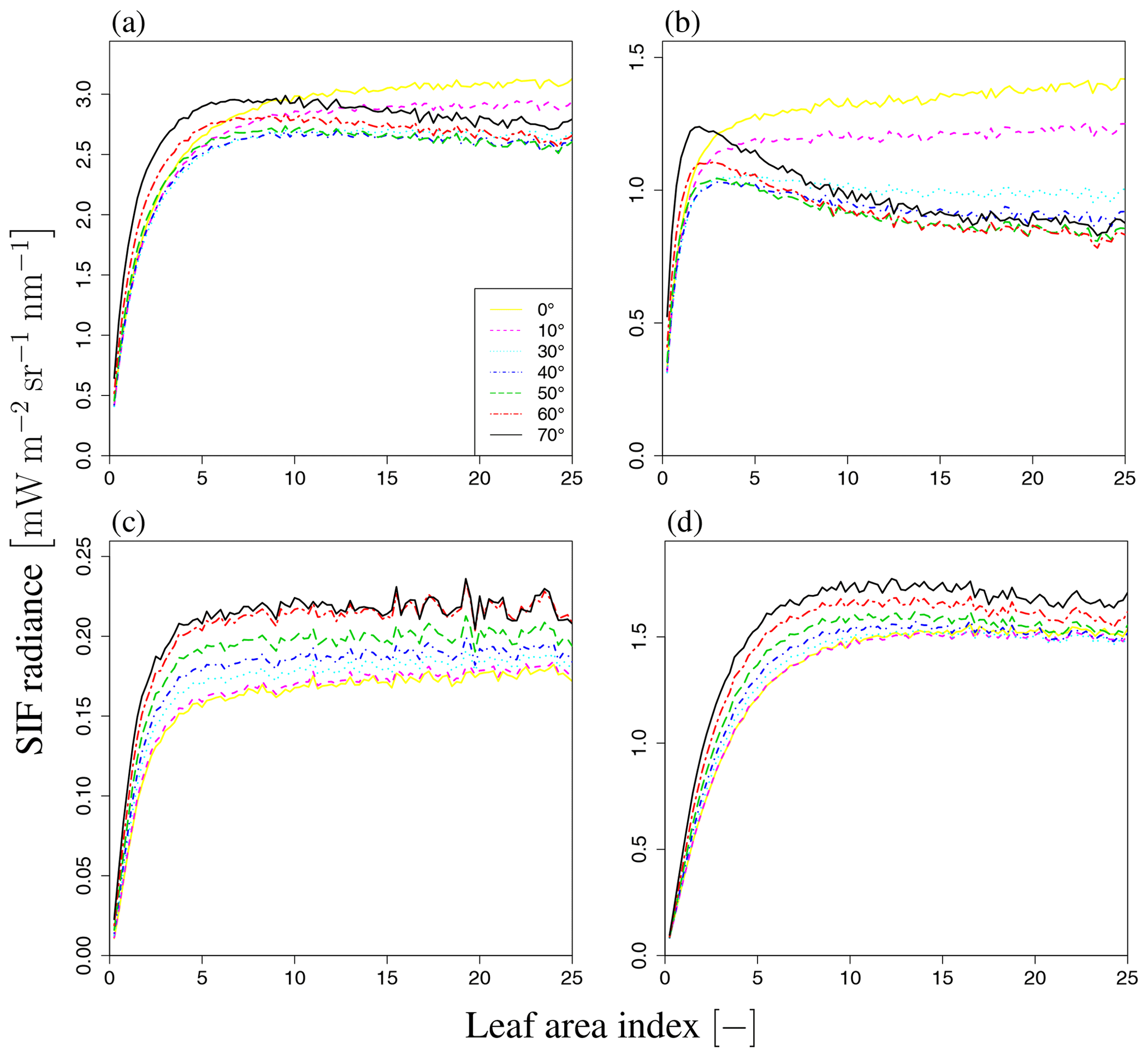
Figure 15LAI dependence of SIF radiance. (a) Total radiance I, (b) direct radiance from sunlit leaves, (c) direct radiance from shaded leaves, and (d) radiance after multiple scatterings at SZA of 20∘ and SAA of 180∘ (backward direction). Each line represents a different VZA value (0–70∘). SIF radiance increases with LAI and then becomes saturated in most cases. However, when VZA is large (e.g., black and red lines), only the direct radiance from sunlit leaves decreases with an increase in LAI, different from the forward direction case.
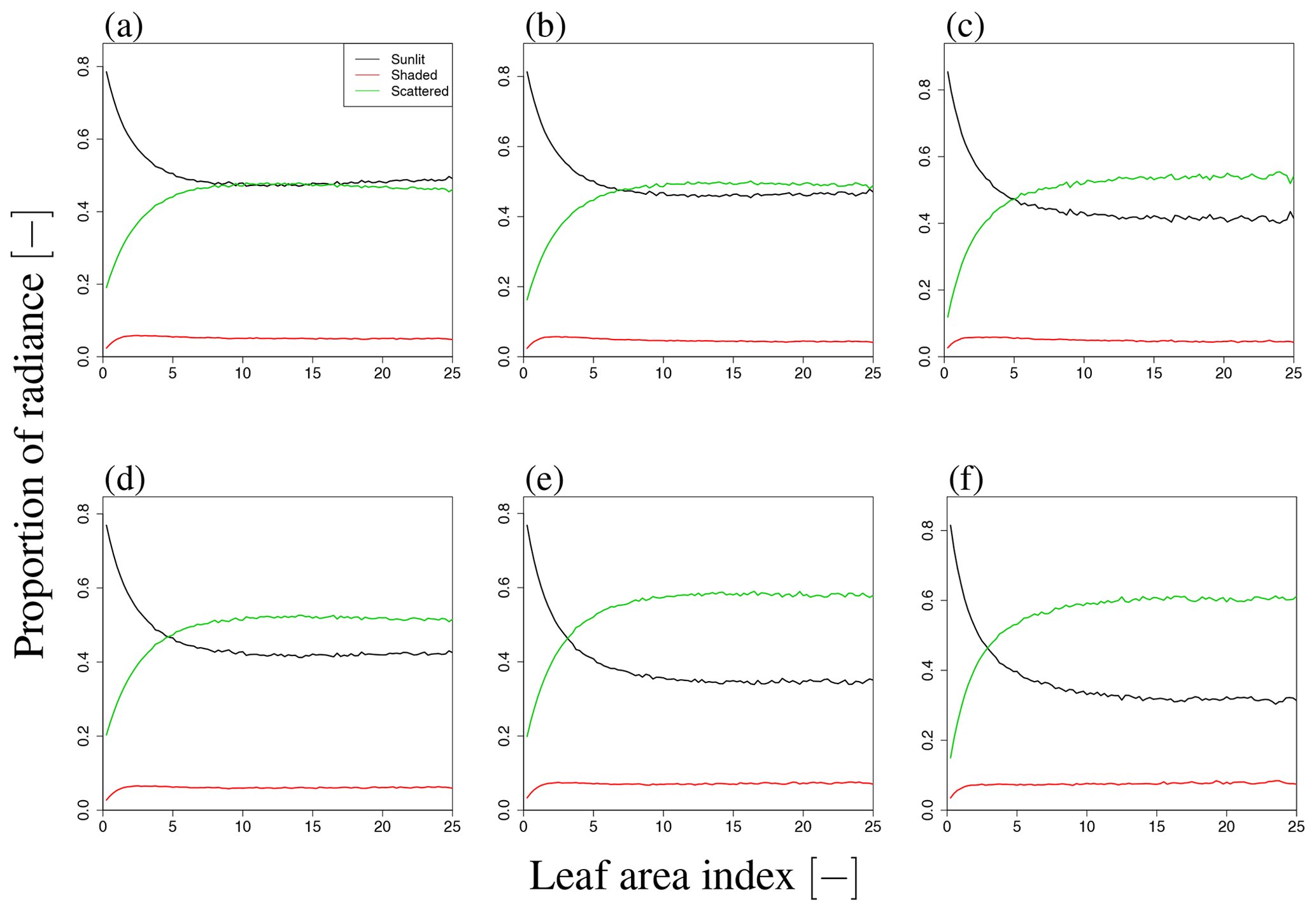
Figure 16Proportion of SIF radiance in LAI variation. Panels (a)–(c) and (d)–(f) indicate results in forward and backward directions, respectively, for different VZA values (10∘ (a, d), 30∘ (b, c), and 50∘ (c, f)). The contribution of shaded leaves is small and the contribution of scattered radiance increases with LAI and VZA. Additionally, in the backward direction, the contribution of scattered radiation to SIF is larger than that in the forward direction, similar to the angular dependency.
Direct SIF radiance from sunlit leaves
The LAI dependency of direct SIF radiance from sunlit leaves is influenced by the hotspot function and the magnitude of VZA (Figs. 14b and 15b). Generally, the SIF radiance emitted from sunlit leaves increases and then saturates as LAI increases, because the number of sunlit leaves also increases and becomes saturated, although the fraction of sunlit leaves decreases (Fig. 17c). However, in terms of simulated SIF radiance, there are ranges of LAI in which SIF radiance decreases with an increase in LAI. In these regions, the decrease in SIF radiance is caused by the attenuation of SIF radiance in the canopy. The magnitude of this attenuation depends on both the hotspot function and VZA. The hotspot function (i.e., the angle αj in Eq. 9) has a major influence on simulated direct SIF radiance from sunlit leaves. The SIF radiance increases and then becomes saturated without decreasing when αj is equal to 0, because the rate of decrease in becomes small when τ=0. Additionally, smaller values of αj produce a smaller rate of decrease in with respect to increases in LAI through the hotspot effect. The magnitude of VZA (i.e., |VZA|) also influences the simulated SIF radiance. Generally, larger LAI values lead to a decrease in the attenuation of SIF radiation from sunlit leaves in the canopy when VZA is positive, because most sunlit leaves inhabit the canopy surface. However, the attenuation of SIF radiation in other canopies increases with |VZA| because of the increase in the pathlength to the canopy boundary when passing through other canopies. The influence of |VZA| and LAI is prominent in negative VZA directions. In this case, the decrease in SIF radiance with an increase in LAI becomes significant because of the SIF emitted through the local canopy to the view point, and the attenuation in the local canopy (and in other canopies) increases with LAI. Thus, the increase in pathlength as |VZA| increases significantly affects in the view direction.

Figure 17Variation of apparent and actual APAR and fraction of sunlit leaves with respect to LAI: (a) apparent APAR, (b) actual APAR, and (c) fraction of sunlit leaves at SZA of 20∘. These variables are not affected by the view direction. APARapp and Fsun decrease exponentially, and APARc increases and then becomes saturated with an increase in LAI.
Direct SIF radiance from shaded leaves
The fraction of shaded leaves has a major influence on SIF radiance. SIF increases and then becomes saturated without decreasing when VZA is negative (Figs. 14c and 15c). This variation in SIF is caused by an increase in the fraction of shaded leaves, because the rate of increase in the fraction is larger than the rate of decrease in . In contrast, the rate of decrease in becomes greater than the rate of increase in the fraction of shaded leaves when VZA is positive. In this region, the expectation of the pathlength to the view point is larger than for negative VZA, because the canopy surface is covered with sunlit leaves. This increase in optical thickness, which depends on the pathlength, has a major effect on in the LAI range where ψ rapidly decreases with any increase in τ′.
Scattered SIF radiance
The scattered SIF radiance refers to the sum of the scattered radiance from sunlit and shaded leaves, , in our model. The LAI dependency with respect to view direction on the scattered SIF radiance is in contrast to the direct radiance from shaded leaves (Figs. 14d and 15d). When VZA is positive, the SIF radiance increases and then becomes saturated without decreasing. The pathlength from sunlit leaves to the population boundary in the view direction has a major influence on simulated scattered SIF radiance. As previously explained (Sect. 3.3.5), the surface of the canopy is covered by sunlit leaves, which provide a large photon weight to scattered photons, in the positive VZA direction. When LAI is large, the decrease in with an increase in LAI becomes vanishingly small. This is because the scattered radiation from high-weight photons reaches the view point with little attenuation. Larger values of LAI lead to shorter scattering path lengths and fewer scatterings, so the photon weight wj is larger. Additionally, the pathlength between sunlit leaves and the boundary of the canopy is nearly constant, irrespective of LAI variation.
The simulated SIF radiance therefore becomes larger than the radiance in the negative VZA direction. Actually, the expectation of the product of w and is larger than when VZA is negative (Fig. 15). In contrast, with an increase in LAI, the SIF radiance decreases and becomes saturated after increasing because of the increase in τ′ from sunlit leaves. This is for a similar reason as for when SZA is negative.
Figure 17 shows APAR and the fraction of sunlit leaves as a function of LAI. APARc increases with an increase in LAI and becomes saturated at around LAI=2. APARapp and the fraction of sunlit leaves decrease when LAI<2. The increase in APARc and the decrease in APARapp are more abrupt than the SIF increase with respect to LAI. This is because APAR is the visible light where the absorption of green leaves is high (∼0.9). Thus, the APARc saturation curve has similar patterns of visible SIF radiance. At higher LAI, the fraction of sunlit leaves is low and APARapp decreases. The statistical accuracy of becomes drastically lower as APARapp and the fraction of sunlit leaves decrease. Accurate simulations of require an increased number of photons to be traced.
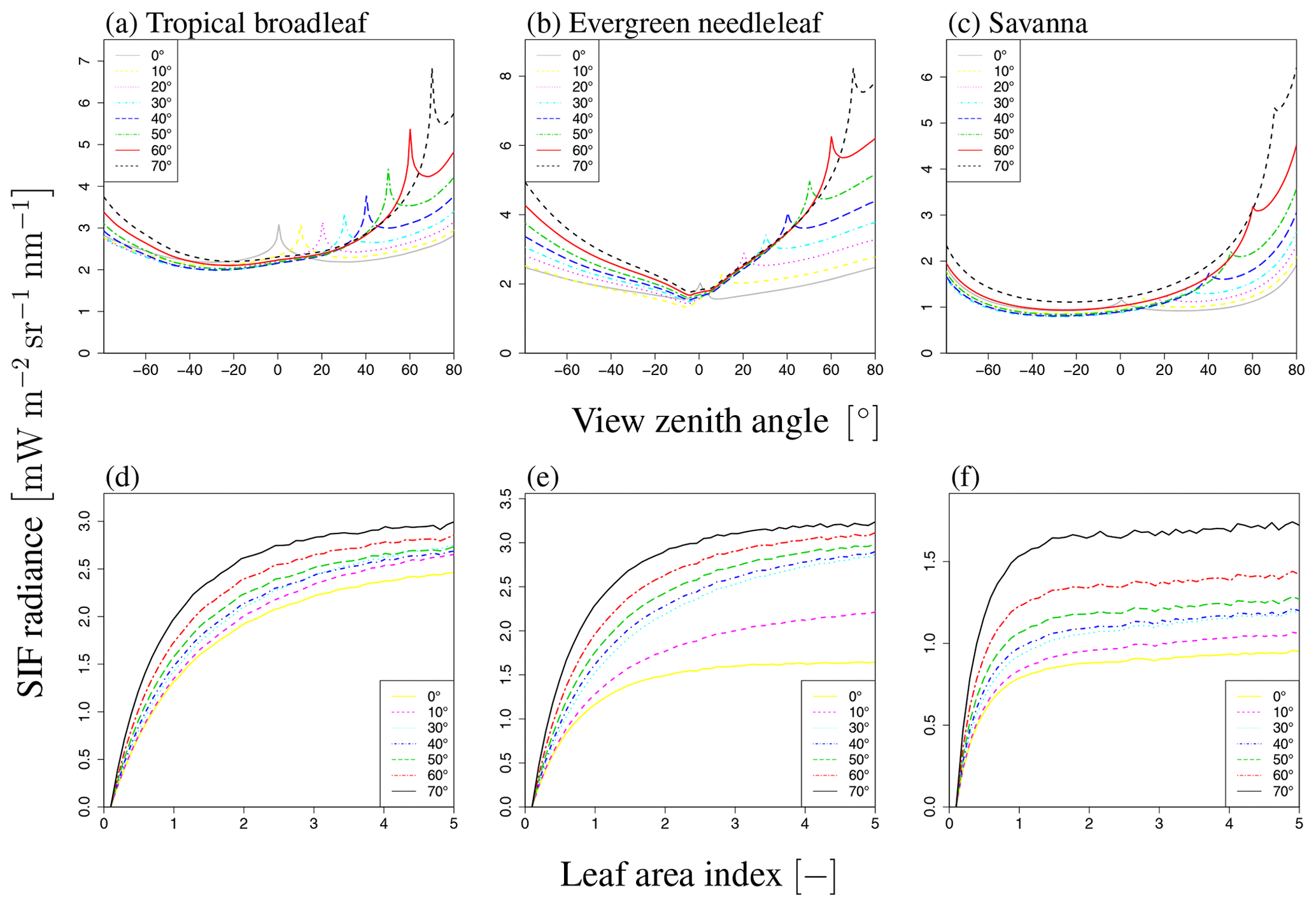
Figure 18Comparison of SIF radiance with different landscapes. Panels (a)–(c) and (d)–(f) indicate VZA dependency (LAI of 3.0) and LAI dependency (VZA of 20∘), respectively. Each line represents a different SZA value (0–70∘).
3.4 Variation of landscape
FLiES-SIF is applicable to a wide variety of landscapes. Figure 18 shows the LAI and SZA dependencies of the total SIF radiation in three different landscapes, namely tropical broadleaf forest, evergreen needle forest, and savanna, which have different tree densities, shapes, and crown coverages (Yang et al., 2018). These simulations use same optical data to demonstrate the applicability of our model. The SIF radiation increases with LAI and then becomes saturated, and there is little difference in LAI dependency among these landscapes (Fig. 18a–c). In contrast, the angular dependency is affected by the landscape composition. For example, in the case of the savanna (Fig. 18c), the hotspot peak is smaller than for the other landscape types because the attenuation within other crowns is reduced by the lower crown coverage.
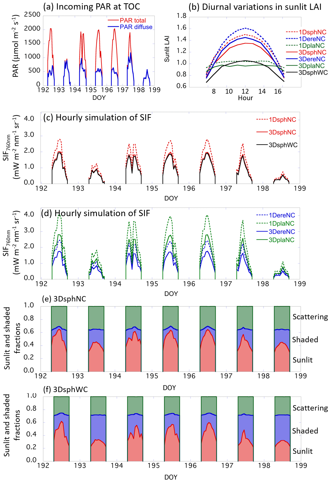
Figure 19Summary of the diurnal SIF variations with actual incident PAR data. (a) Incoming total and diffuse PAR at the top of canopy (TOC). The observed PAR data in photon units () are converted to the unit of energy unit (W m−2) for the SIF simulation. (b) Diurnal variations in sunlit LAI for different canopy structures. In all scenarios, total LAIs were set to 3. (c) Simulated SIF radiances on hourly timescales for 1DsphNC, 3DsphNC, and 3DsphWC. (d) Simulated SIF radiances on hourly timescales for 1DereNC, 1DplaNC, 3DereNC, and 3DplaNC. Dotted lines are 1-D scenarios and solid lines are the results of 3-D scenarios. (e) The fraction of sunlit, shaded, and scattering contributions in the simulated total SIF radiance for 3DsphNC (no clumping). (f) The fraction of sunlit, shaded, and scattering contributions in the simulated total SIF radiance for 3DsphWC (within-crown clumping).
3.5 Comparison of 1-D and 3-D actual diurnal variations in PAR
Simulations with a 1 h step size were performed using observed total and diffuse PAR data from Yokohama, Japan, from 12 to 18 July (DOY 192–198) 2014 (Fig. 19a). This period included clear-sky days (DOY 192, 195, and 196) and overcast days (DOY 193, 198). The LAI value was fixed to 3.0 throughout the simulation period in all scenarios. The diurnal variations in sunlit LAI show distinct features with respect to 1-D and 3-D landscapes, as well as to the leaf angle distribution (Fig. 19b). In summary, the simulated sunlit LAIs in the 1-D scenarios (1DsphNC, 1DereNC, 1DplaNC) are higher than those in the 3-D scenarios (3DsphNC, 3DereNC, 3DplaNC, 3DsphWC), and the difference in the leaf angle distribution affects the diurnal feature of sunlit LAI significantly: erectrophile cases give the highest values, followed by spherical, and then planophile. The planophile cases (1DplaNC, 3DplaNC) exhibit weak diurnal variations because of the high probability of horizontal leaves: the uppermost leaves receive most of the incoming light, regardless of SZA. The sunlit LAI of the within-crown clumping scenario (3DsphWC) is significantly lower than in the no-clumping scenario (3DsphNC, 29.7 % lower at noon). Figure 19c and d show the hourly simulation results for the top-of-canopy SIF at 760 nm.
The simulated SIF generally follows the diurnal variations in incoming PAR; however, the absolute range varies greatly depending on the leaf angle distribution (spherical, erectrophile, or planophile) and in the 1-D and 3-D cases. For example, the canopy SIF simulated by 1DplaNC is 2.3 times higher than that of 3DereNC at noon on a clear day (DOY 192). In contrast, the simulated SIF differences are minor on overcast days (DOY 193, 198). The simulated results also indicate that there is a sort of “trade-off” relationship between the amount of sunlit LAI and SIF: the SIF values simulated by planophile scenarios (1DplaNC, 3DplaNC) are higher than those in erectrophile scenarios (1DereNC, 3DereNC), while the amount of sunlit LAI in planophile scenarios is lower than that in erectrophile scenarios. This is because leaves with an erectrophile distribution receive the solar beam efficiently as they have a large proportion of vertical leaves. This, in turn, results in larger incident angles of the solar beam on the leaf surfaces, which reduces the incident PAR intensity on the unit leaf area. Comparing the 3-D scenarios with the 1-D scenarios, the latter simulated the SIF to be 33 %–41 % higher than the former.
Additionally, we investigated the contribution of direct SIF from sunlit leaves (Idir_sun), shaded leaves (Idir_shade), and multiple scattering components (Ims_sun+Ims_shade) (Fig. 19e and f). The largest contribution comes from sunlit leaves. The contribution from shaded leaves is generally lower than that from sunlit leaves, although on overcast days (DOY 193 and 198) the contribution becomes close to or even higher than that of the sunlit leaves (Fig. 19e and f). Multiple scattering contributes substantially in the near-infrared domain (30 %–40 % of total SIF radiance) but is expected to make a lower contribution in the red spectrum because of low leaf reflectance and transmittance. A comparison of 3DsphNC and 3DsphWC shows that the shaded leaves of the within-crown clumping scenario contribute more to the total SIF than those in the no-clumping scenario. Overall, the 1-D and 3-D comparisons, as well as differences in leaf angle distributions, suggest that reasonable assumptions must be made regarding the canopy structure if the SIF simulations are to be reliable. If 1-D models are applied to forest canopies, the simulated SIF is prone to be overestimated.
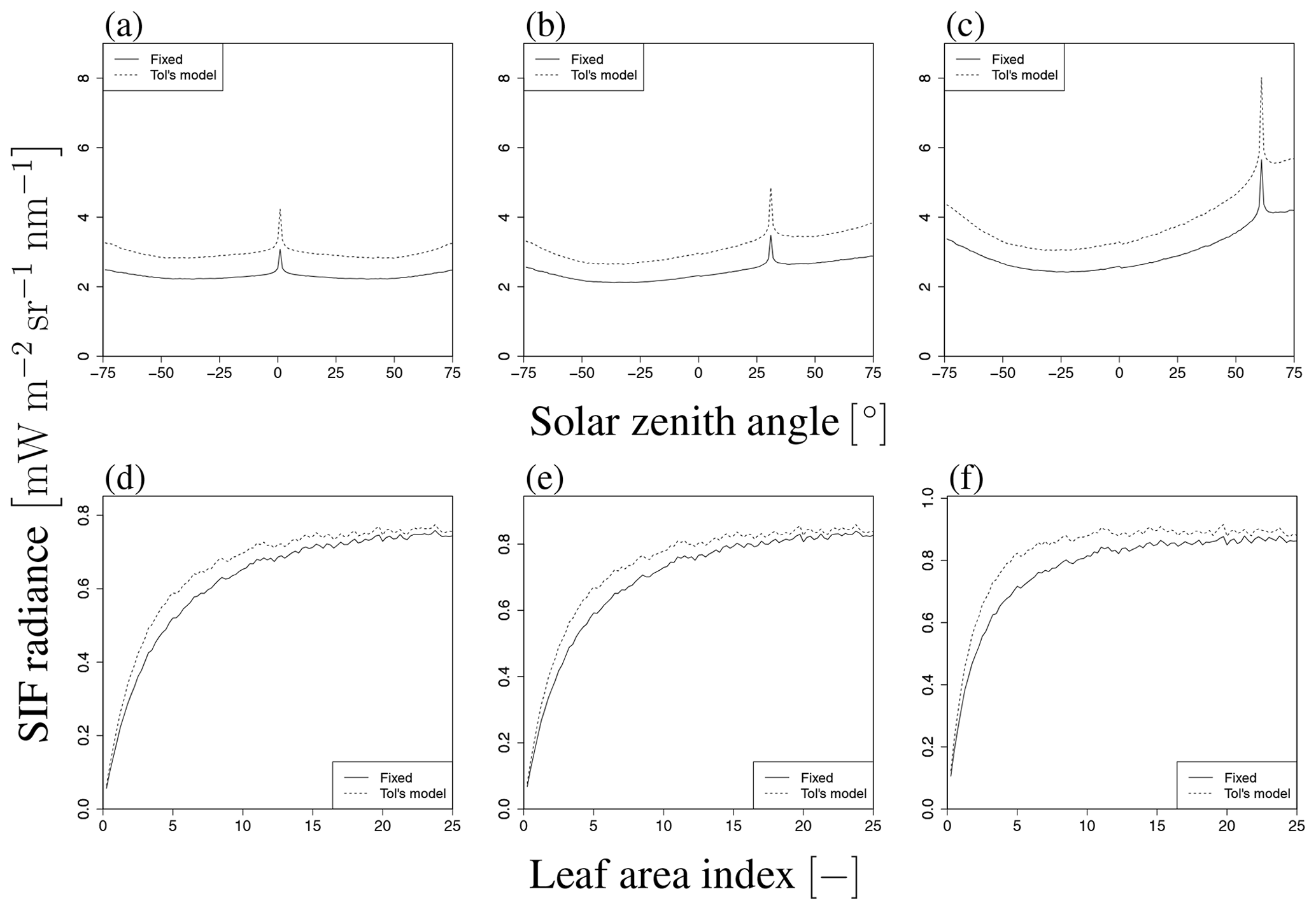
Figure 20Comparison of SIF radiance with different ϕf (constant and from Tol's model). Upper and lower figures indicate SZA dependency (LAI=3.0) and LAI dependency (SZA of 20∘), respectively. The VZA values are 0∘ (a, d), 30∘ (b, e), and 60∘ (c, f). The solid line indicates the case of constant ϕf (=0.01). The dashed line indicates the result of Tol's model, where ϕf depends on APARL, as shown in Fig. 8.
3.6 Influence of fluorescence yield on variable APARL scenario
Figure 20 compares the total SIF derived from fixed and variable leaf-level SIF yields. To explore the influence of the SIF yield on the above dependencies, we derive ϕf by means of Tol's model (van der Tol et al., 2014) to calculate the yield from APAR, which is obtained by our model (Fig. 8). Additionally, we obtain the photosynthesis yield by Farquhar's model using parameter values set by reference of previous literatures (such as van der Tol et al., 2014; De Pury and Farquhar, 1997) to derive the ϕf without observation data. Figure 20 compares the total SIF radiance I between models based on constant ϕf and APAR-dependent ϕf in terms of their dependence on LAI and SZA, respectively. The dependency on the two parameters is not substantially different because the variation in ϕf is smaller than that of APAR. However, ϕf affects APARapp as well as the bidirectional SIF radiance. Thus, obtaining accurate values of ϕf is important in estimating the exact level of SIF; this issue will be considered in future work.
In this paper, we have described the structure of FLiES-SIF version 1.0 and the simulation algorithm for canopy-scale Sun-induced chlorophyll fluorescence emissions. The model was developed by extending the original FLiES model. FLiES-SIF is based on the Monte Carlo ray-tracing approach. The SIF emissions from sunlit and shaded leaves are computed separately, and the model also considers multiple scatterings within forest canopies. FLiES-SIF version 1.0 simulates virtual forest landscapes, where individual tree positions and crown dimensions are explicitly considered. Therefore, the model can examine the influence of various ecological and environmental factors (e.g., forest structures and solar direction) on SIF emissions in a realistic canopy. A 3-D radiative transfer modeling approach is necessary for understanding the biological and physical mechanisms behind the SIF emissions from complex forest canopies. We performed a test run to demonstrate the sensitivity of SIF to the view angle, LAI, and leaf-level SIF yield. The simulation results show that SIF increases with LAI before becoming saturated when LAI>2–4, depending on the spectral wavelength. The sensitivity analyses also showed that simulated SIF radiation may decrease with LAI when LAI>5. These phenomena were observed under certain Sun and view angle conditions. This type of nonlinear and nonmonotonic SIF behavior is also related to the spatial forest structure patterns and leaf angle distributions. The simulated SIF with a 1-D canopy assumption is prone to be overestimated. The hotspot effect plays an important role in SIF simulations when the view direction is close to the Sun direction. The SIF yield ϕf influences the canopy SIF, especially when APAR is low. FLiES-SIF version 1.0 can be used to quantify the canopy SIF at various view angles, including the contribution of multiple scatterings, which is an important component in the near-infrared domain. The proposed model can be used to standardize satellite SIF by correcting the bidirectional effect. This step will contribute to improved GPP estimation accuracy through SIF. In this model description paper, we have focused on the formulation and simulation schemes of FLiES-SIF version 1.0, and have presented the results from sensitivity analyses of major variables such as LAI. Model validation using field measurements will be performed in future studies. Thorough validation against measured quantities should be conducted to evaluate the accuracy of the model.
The FLiES-SIF version 1.0 source code and sample data sets used in this study are publicly available through Zenodo (Kobayashi and Sakai, 2019, https://doi.org/10.5281/zenodo.3584099). The source codes are written in Fortran (gfortran), C (gcc) and R script. This is an open source software under the agreement of Creative Commons Attribution 4.0 International license (CC BY 4.0).
YS, HK, and TK designed the FLiES-SIF version 1.0 model. YS and HK developed the FLiES-SIF version 1.0. YS carried out the sensitivity analysis. YS and HK wrote the paper.
The authors declare that they have no conflict of interest.
We thank Jean-Philippe Gastellu-Etchegorry for his kind support and instructive advice in running the DART-SIF module. FLiES-SIF version 1.0 development was supported by the Environment Research and Technology Development Fund (2RF-1601, 2-1903) and JSPS Kakenhi (25281014, 16H02948, 18H03350). We thank Stuart Jenkinson, PhD, from Edanz Group (https://en-author-services.edanzgroup.com/, last access: 2 July 2020) for making English language changes on a draft of this paper.
This research has been supported by the Environment Research and Technology Development Fund (grant nos. 2RF-1601 and 2-1903) and the JSPS Kakenhi (grant nos. 25281014, 16H02948, and 18H03350).
This paper was edited by Christoph Müller and reviewed by two anonymous referees.
Agati, G., Fusi, F., Mazzinghi, P., and di Paola, M. L.: A simple approach to the evaluation of the reabsorption of chlorophyll fluorescence spectra in intact leaves, J. Photoch. Photobiol. B, 17, 163–171, 1993. a, b
Anav, A., Friedlingstein, P., Beer, C., Ciais, P., Harper, A., Jones, C., Murray-Tortarolo, G., Papale, D., Parazoo, N. C., Peylin, P., Piao, S., Sitch, S., Viovy, N., Wiltshire, A., and Zhao, M.: Spatiotemporal patterns of terrestrial gross primary production: A review, Rev. Geophys., 53, 785–818, 2015. a
Antyufeev, V. S. and Marshak, A. L.: Monte Carlo method and transport equation in plant canopies, Remote Sens. Environ., 31, 183–191, 1990. a, b
Baldocchi, D. and Harley, P.: Scaling carbon dioxide and water vapour exchange from leaf to canopy in a deciduous forest. II. Model testing and application, Plant Cell Environ., 18, 1157–1173, 1995. a
Bunn, A. G. and Goetz, S. J.: Trends in satellite-observed circumpolar photosynthetic activity from 1982 to 2003: the influence of seasonality, cover type, and vegetation density, Earth Interact., 10, 1–19, 2006. a
Canadell, J. G., Kirschbaum, M. U., Kurz, W. A., Sanz, M.-J., Schlamadinger, B., and Yamagata, Y.: Factoring out natural and indirect human effects on terrestrial carbon sources and sinks, Environ. Sci. Policy, 10, 370–384, 2007. a
Cescatti, A. and Zorer, R.: Structural acclimation and radiation regime of silver fir (Abies alba Mill.) shoots along a light gradient, Plant Cell Environ., 26, 429–442, 2003. a, b
Chen, J. M., Rich, P. M., Gower, S. T., Norman, J. M., and Plummer, S.: Leaf area index of boreal forests: Theory, techniques, and measurements, J. Geophys. Res.-Atmos., 102, 29429–29443, 1997. a
Collatz, G. J., Ball, J. T., Grivet, C., and Berry, J. A.: Physiological and environmental regulation of stomatal conductance, photosynthesis and transpiration: a model that includes a laminar boundary layer, Agric. Forest Meteorol., 54, 107–136, 1991. a
Dang, Q.-L., Margolis, H. A., Coyea, M. R., Sy, M., and Collatz, G. J.: Regulation of branch-level gas exchange of boreal trees: roles of shoot water potential and vapor pressure difference, Tree Physiol., 17, 521–535, 1997. a, b, c, d
Dechant, B., Ryu, Y., Badgley, G., Zeng, Y., Berry, J. A., Zhang, Y., Goulas, Y., Li, Z., Zhang, Q., Kang, M., Li, J., and Moya, I.: Canopy structure explains the relationship between photosynthesis and sun-induced chlorophyll fluorescence in crops, Remote Sens. Environ., 241, 111733, 2020. a
De Pury, D. and Farquhar, G.: Simple scaling of photosynthesis from leaves to canopies without the errors of big-leaf models, Plant Cell Environ., 20, 537–557, 1997. a, b
Farquhar, G. D., von Caemmerer, S. V., and Berry, J. A.: A biochemical model of photosynthetic CO2 assimilation in leaves of C3 species, Planta, 149, 78–90, 1980. a, b, c
Frankenberg, C., Butz, A., and Toon, G.: Disentangling chlorophyll fluorescence from atmospheric scattering effects in O2 A-band spectra of reflected sun-light, Geophys. Res. Lett., 38, 2011. a, b
Gastellu-Etchegorry, J.-P., Lauret, N., Yin, T., Landier, L., Kallel, A., Malenovsk, Z., Al Bitar, A., Aval, J., Benhmida, S., Qi, J., Medjdoub, G., Guilleux, J., Chavanon, E., Cook, B., Morton, D., Chrysoulakis, N., and Mitraka, Z.: DART: recent advances in remote sensing data modeling with atmosphere, polarization, and chlorophyll fluorescence, IEEE J. Sel. Top. Appl., 10, 2640–2649, 2017. a, b, c
Genty, B., Briantais, J.-M., and Baker, N. R.: The relationship between the quantum yield of photosynthetic electron transport and quenching of chlorophyll fluorescence, Biochim. Biophys. Ac., 990, 87–92, 1989. a
Guanter, L., Alonso, L., Gómez-Chova, L., Meroni, M., Preusker, R., Fischer, J., and Moreno, J.: Developments for vegetation fluorescence retrieval from spaceborne high-resolution spectrometry in the O2-A and O2-B absorption bands, J. Geophys. Res.-Atmos., 115, D19303, https://doi.org/10.1029/2009JD013716, 2010. a
Hapke, B.: Theory of reflectance and emittance spectroscopy, Cambridge University Press, 2012. a
Hernández-Clemente, R., North, P. R., Hornero, A., and Zarco-Tejada, P. J.: Assessing the effects of forest health on sun-induced chlorophyll fluorescence using the FluorFLIGHT 3-D radiative transfer model to account for forest structure, Remote Sens. Environ., 193, 165–179, 2017. a
Iwabuchi, H.: Efficient Monte Carlo methods for radiative transfer modeling, J. Atmos. Sci., 63, 2324–2339, 2006. a
Joiner, J., Guanter, L., Lindstrot, R., Voigt, M., Vasilkov, A. P., Middleton, E. M., Huemmrich, K. F., Yoshida, Y., and Frankenberg, C.: Global monitoring of terrestrial chlorophyll fluorescence from moderate-spectral-resolution near-infrared satellite measurements: methodology, simulations, and application to GOME-2, Atmos. Meas. Tech., 6, 2803–2823, https://doi.org/10.5194/amt-6-2803-2013, 2013. a, b
Kobayashi, H.: Directional effect of canopy scale sun-induced chlorophyll fluorescence: Theoretical Consideration in A3-D radiative transfer model, in: 2015 IEEE Int. Geosci. Remote Se., pp. 3413–3415, 2015a. a
Kobayashi, H.: Leaf, woody and background optical data for GCOM-C LAI/FAPAR retrieval, JAXA GCOM-C RA4, 102, 2015b. a, b
Kobayashi, H.: FLiES version 2.9, Zenodo, https://doi.org/10.5281/zenodo.3586814, 2019. a
Kobayashi, H. and Iwabuchi, H.: A coupled 1-D atmosphere and 3-D canopy radiative transfer model for canopy reflectance, light environment, and photosynthesis simulation in a heterogeneous landscape, Remote Sens. Environ., 112, 173–185, 2008. a, b, c, d, e, f, g, h
Kobayashi, H. and Sakai, Y.: FLiES-SIF version 1.0, Zenodo, https://doi.org/10.5281/zenodo.3584099, 2019. a, b
Kobayashi, H., Delbart, N., Suzuki, R., and Kushida, K.: A satellite-based method for monitoring seasonality in the overstory leaf area index of Siberian larch forest, J. Geophys. Res.-Biogeo., 115, G01002, https://doi.org/10.1029/2009JG000939, 2010. a, b
Kobayashi, H., Baldocchi, D. D., Ryu, Y., Chen, Q., Ma, S., Osuna, J. L., and Ustin, S. L.: Modeling energy and carbon fluxes in a heterogeneous oak woodland: A three-dimensional approach, Agric. Forest Meteorol., 152, 83–100, 2012. a, b
Köhler, P., Frankenberg, C., Magney, T. S., Guanter, L., Joiner, J., and Landgraf, J.: Global retrievals of solar-induced chlorophyll fluorescence with TROPOMI: First results and intersensor comparison to OCO-2, Geophys. Res. Lett., 45, 10–456, 2018. a
Lasslop, G., Reichstein, M., Papale, D., Richardson, A. D., Arneth, A., Barr, A., Stoy, P., and Wohlfahrt, G.: Separation of net ecosystem exchange into assimilation and respiration using a light response curve approach: critical issues and global evaluation, Global Change Biol., 16, 187–208, 2010. a
Li, X., Xiao, J., He, B., Altaf Arain, M., Beringer, J., Desai, A. R., Emmel, C., Hollinger, D. Y., Krasnova, A., Mammarella, I., Noe, S. M., Ortiz, P. S., Ray-Sanchez. A. C., Rocha, A. V., and Varlagin, A.: Solar-induced chlorophyll fluorescence is strongly correlated with terrestrial photosynthesis for a wide variety of biomes: First global analysis based on OCO-2 and flux tower observations, Global Change Biol., 24, 3990–4008, 2018. a
Liu, X., Guanter, L., Liu, L., Damm, A., Malenovskỳ, Z., Rascher, U., Peng, D., Du, S., and Gastellu-Etchegorry, J.-P.: Downscaling of solar-induced chlorophyll fluorescence from canopy level to photosystem level using a random forest model, Remote Sens. Environ., 231, 110772, https://doi.org/10.1016/j.rse.2018.05.035, 2019. a
Louis, J., Cerovic, Z. G., and Moya, I.: Quantitative study of fluorescence excitation and emission spectra of bean leaves, J. Photoch. Photobiol. B, 85, 65–71, 2006. a
Marchuk, G. I., Mikhailov, G. A., Nazareliev, M., Darbinjan, R. A., Kargin, B. A., and Elepov, B. S.: The Monte Carlo methods in atmospheric optics, vol. 1, Springer, 1980. a
Norton, A. J., Rayner, P. J., Koffi, E. N., Scholze, M., Silver, J. D., and Wang, Y.-P.: Estimating global gross primary productivity using chlorophyll fluorescence and a data assimilation system with the BETHY-SCOPE model, Biogeosciences, 16, 3069–3093, https://doi.org/10.5194/bg-16-3069-2019, 2019. a
Pedrós, R., Goulas, Y., Jacquemoud, S., Louis, J., and Moya, I.: FluorMODleaf: A new leaf fluorescence emission model based on the PROSPECT model, Remote Sens. Environ., 114, 155–167, 2010. a, b, c, d
Piao, S., Sitch, S., Ciais, P., Friedlingstein, P., Peylin, P., Wang, X., Ahlström, A., Anav, A., Canadell, J. G., Cong, N., Huntingford, C., Jung, M. Levis, S., Levy, P. E., Li, J., Lin, X., Lomas, M. R., Lu, M., Luo, Y., Ma, Y., Myneni, R. B., Poulter, B., Sun, Z., Wang, T., Viovy, N., Zaehle, S., and Zeng, N.: Evaluation of terrestrial carbon cycle models for their response to climate variability and to CO2 trends, Global Change Biol., 19, 2117–2132, 2013. a
Porcar-Castell, A., Tyystjärvi, E., Atherton, J., Van der Tol, C., Flexas, J., Pfündel, E. E., Moreno, J., Frankenberg, C., and Berry, J. A.: Linking chlorophyll a fluorescence to photosynthesis for remote sensing applications: mechanisms and challenges, J. Exp. Bot., 65, 4065–4095, 2014. a, b
Richardson, A. D., Hollinger, D. Y., Dail, D. B., Lee, J. T., Munger, J. W., and O'Keefe, J.: Influence of spring phenology on seasonal and annual carbon balance in two contrasting New England forests, Tree Physiol., 29, 321–331, 2009. a
Romero, J. M., Cordon, G. B., and Lagorio, M. G.: Modeling re-absorption of fluorescence from the leaf to the canopy level, Remote Sens. Environ., 204, 138–146, 2018. a
Schimel, D.: Carbon cycle conundrums, P. Natl. Acad. Sci., 104, 18353–18354, 2007. a
Smolander, S. and Stenberg, P.: A method to account for shoot scale clumping in coniferous canopy reflectance models, Remote Sens. Environ., 88, 363–373, 2003. a
Smolander, S. and Stenberg, P.: Simple parameterizations of the radiation budget of uniform broadleaved and coniferous canopies, Remote Sens. Environ., 94, 355–363, 2005. a
Teubner, I. E., Forkel, M., Camps-Valls, G., Jung, M., Miralles, D. G., Tramontana, G., van der Schalie, R., Vreugdenhil, M., Mösinger, L., and Dorigo, W. A.: A carbon sink-driven approach to estimate gross primary production from microwave satellite observations, Remote Sens. Environ., 229, 100–113, 2019. a
van der Tol, C., Verhoef, W., Timmermans, J., Verhoef, A., and Su, Z.: An integrated model of soil-canopy spectral radiances, photosynthesis, fluorescence, temperature and energy balance, Biogeosciences, 6, 3109–3129, https://doi.org/10.5194/bg-6-3109-2009, 2009. a, b, c, d
van der Tol, C., Berry, J., Campbell, P., and Rascher, U.: Models of fluorescence and photosynthesis for interpreting measurements of solar-induced chlorophyll fluorescence, J. Geophys. Res.-Biogeo., 119, 2312–2327, 2014. a, b, c, d, e, f, g, h
van der Tol, C., Vilfan, N., Dauwe, D., Cendrero-Mateo, M. P., and Yang, P.: The scattering and re-absorption of red and near-infrared chlorophyll fluorescence in the models Fluspect and SCOPE, Remote Sens. Environ., 232, 111292, https://doi.org/10.1016/j.rse.2019.111292, 2019. a
Van Wittenberghe, S., Alonso, L., Verrelst, J., Moreno, J., and Samson, R.: Bidirectional sun-induced chlorophyll fluorescence emission is influenced by leaf structure and light scattering properties-A bottom-up approach, Remote Sens. Environ., 158, 169–179, 2015. a
Waring, R., Landsberg, J., and Williams, M.: Net primary production of forests: a constant fraction of gross primary production?, Tree Physiol., 18, 129–134, 1998. a
Widlowski, J.-L., Pinty, B., Clerici, M., Dai, Y., De Kauwe, M., De Ridder, K., Kallel, A., Kobayashi, H., Lavergne, T., Ni-Meister, W., Olchev, A., Quaife, T., Wang, S., Yang, W., Yang, Y., and Yuan, H: RAMI4PILPS: An intercomparison of formulations for the partitioning of solar radiation in land surface models, J. Geophys. Res.-Biogeo., 116, G02019, https://doi.org/10.1029/2010JG001511, 2011. a
Widlowski, J.-L., Pinty, B., Lopatka, M., Atzberger, C., Buzica, D., Chelle, M., Disney, M., Gastellu-Etchegorry, J.-P., Gerboles, M., Gobron, N., Grau, E., Huang, H., Kobayashi, H., Lewis, P. E., Qin, W., Schlerf, M., Stuckens, J., and Xie, D.: The fourth radiation transfer model intercomparison (RAMI-IV): Proficiency testing of canopy reflectance models with ISO-13528, J. Geophys. Res.-Atmos., 118, 6869–6890, 2013. a
Widlowski, J.-L., Mio, C., Disney, M., Adams, J., Andredakis, I., Atzberger, C., Brennan, J., Busetto, L., Chelle, M., Ceccherini, G., Colombo, R., Côté, J.-F., Eenmäe, A., Essery , R., Gastellu-Etchegorry, J.-P., Gobron, N., Grau, E., Haverd, V., Homolová, L., Huang, H., Hunt, L., Kobayashi, H., Koetz, B., Kuusk, A., Kuusk, J., Lang, M., Lewis, P. E., Lovell, J. L., Malenovský, Z., Meroni, M., Morsdorf, F., Mõttus, M., Ni-Meister, W., Pinty, B., Rautiainen, M., Schlerf, M., Somers, B., Stuckens, J., Verstraete, M. M., Yang. W., Zhao, F., and Zenone, T.: The fourth phase of the radiative transfer model intercomparison (RAMI) exercise: Actual canopy scenarios and conformity testing, Remote Sens. Environ., 169, 418–437, 2015. a
Wieneke, S., Burkart, A., Cendrero-Mateo, M., Julitta, T., Rossini, M., Schickling, A., Schmidt, M., and Rascher, U.: Linking photosynthesis and sun-induced fluorescence at sub-daily to seasonal scales, Remote Sens. Environ., 219, 247–258, 2018. a
Wu, J., Kobayashi, H., Stark, S. C., Meng, R., Guan, K., Tran, N. N., Gao, S., Yang, W., Restrepo-Coupe, N., Miura, T., Oliviera, R. C., Rogers, A., Dye, D. G., Nelson, B. W., Serbin, S. P., Huete, A. R., and Saleska, S. R.: Biological processes dominate seasonality of remotely sensed canopy greenness in an Amazon evergreen forest, New Phytol., 217, 1507–1520, 2018. a
Yang, P. and van der Tol, C.: Linking canopy scattering of far-red sun-induced chlorophyll fluorescence with reflectance, Remote Sens. Environ., 209, 456–467, 2018. a
Yang, W., Kobayashi, H., Chen, X., Nasahara, K. N., Suzuki, R., and Kondoh, A.: Modeling three-dimensional forest structures to drive canopy radiative transfer simulations of bidirectional reflectance factor, Int. J. Digit. Earth, 11, 981–1000, 2018. a, b
Zarco-Tejada, P. J., Miller, J. R., Pedrós, R., Verhoef, W., and Berger, M.: FluorMODgui V3. 0: A graphic user interface for the spectral simulation of leaf and canopy chlorophyll fluorescence, Comput. Geosci., 32, 577–591, 2006. a, b, c
Zarco-Tejada, P. J., Suárez, L., and González-Dugo, V.: Spatial resolution effects on chlorophyll fluorescence retrieval in a heterogeneous canopy using hyperspectral imagery and radiative transfer simulation, IEEE Geosci. Remote Sens. Lett., 10, 937–941, 2013. a
Zeng, Y., Badgley, G., Dechant, B., Ryu, Y., Chen, M., and Berry, J. A.: A practical approach for estimating the escape ratio of near-infrared solar-induced chlorophyll fluorescence, Remote Sens. Environ., 232, 111209, https://doi.org/10.1016/j.rse.2019.05.028, 2019. a
Zhang, Y., Guanter, L., Joiner, J., Song, L., and Guan, K.: Spatially-explicit monitoring of crop photosynthetic capacity through the use of space-based chlorophyll fluorescence data, Remote Sens. Environ., 210, 362–374, 2018. a