An exploratory performance assessment of the CHIMERE model (version 2017r4) for the northwestern Iberian Peninsula and the summer season

Here, the capability of the chemical weather forecasting model CHIMERE (version 2017r4) to reproduce surface ozone, particulate matter and nitrogen dioxide concentrations in complex terrain is investigated for the period from 21 June to 21 August 2018. The study area is the northwestern Iberian Peninsula, where both coastal and mountain climates can be found in direct vicinity and a large fraction of the land area is covered by forests. Driven by lateral boundary conditions from the European Centre for Medium-Range Weather Forecasts (ECMWF) Composition Integrated Forecast System, anthropogenic emissions from two commonly used top-down inventories and meteorological data from the Weather Research and Forecasting Model, CHIMERE's performance with respect to observations is tested with a range of sensitivity experiments. We assess the effects of (1) an increase in horizontal resolution, (2) an increase in vertical resolution, (3) the use of distinct model chemistries, and (4) the use of distinct anthropogenic emissions inventories, downscaling techniques and land use databases. In comparison with the older HTAP emission inventory downscaled with basic options, the updated and sophistically downscaled EMEP inventory only leads to partial model improvements, and so does the computationally costly horizontal resolution increase. Model performance changes caused by the choice of distinct chemical mechanisms are not systematic either and rather depend on the considered anthropogenic emission configuration and pollutant. Although the results are thus heterogeneous in general terms, the model's response to a vertical resolution increase confined to the lower to middle troposphere is homogeneous in the sense of improving virtually all verification aspects. For our study region and the two aforementioned top-down emission inventories, we conclude that it is not necessary to run CHIMERE on a horizontal mesh much finer than the native grid of these inventories. A relatively coarse horizontal mesh combined with 20 model layers between 999 and 500 hPa is sufficient to yield balanced results. The chemical mechanism should be chosen as a function of the intended application.

1 Introduction

Motivated by the air quality legislation of the European Union (EU, 2008), many governmental air quality departments are currently demanding air quality forecasting schemes based on numerical models (Thunis et al., 2016), and the need for accurate and computationally efficient predictions in this field is perhaps greater than ever before. For Europe as a whole, the most important real-time prediction system available to date is provided by the Copernicus Atmosphere Monitoring Service (Marécal et al., 2015), currently comprising an ensemble of seven chemical weather forecasting (CWF) models¹ run for the entire continent at a horizontal resolution of 0.1 to 0.25^∘ in longitude and 0.1 to 0.2^∘ in latitude. In addition to this short-term prediction system, several large research initiatives have been issued during the last 2 decades in order to assess the climatological properties of atmospheric composition, including the detection of long-term trends resulting from emission reductions induced by the Convention on Long-range Transboundary Air Pollution (CLRTAP, 2019). The final aim of these efforts is to find model configurations, or ensembles thereof, that can be used as surrogates for real observations in order to assess whether emission reductions actually have lead, or would lead, to changes in the atmosphere's composition on climatological timescales (Vautard et al., 2006; Jonson et al., 2006; Colette et al., 2011, 2017; Wilson et al., 2012; Banzhaf et al., 2015; Im et al., 2018b, a; Vivanco et al., 2018; Theobald et al., 2019).

Complementary to these large-scale efforts, usually conducted with a single configuration of a given model (Bessagnet et al., 2016), small-scale sensitivity tests for particular models are still relevant since they can be run with more sophisticated model configurations than their large-scale counterparts and are therefore more interesting for regional prediction systems, such as those demanded by national or regional governments (Banzhaf et al., 2012; Beegum et al., 2016; Flamant et al., 2018). Further, following the concept of seamless prediction (Palmer et al., 2008), lessons learned from short-term prediction systems for relatively small geographical areas might also be important for longer lead times and larger areas.

Previous sensitivity studies have identified several factors influencing model capability to correctly reproduce observed values, hereafter referred to as “model performance” (Giorgi and Francisco, 2000; Chang and Hanna, 2004). Among these factors, the meteorological model used to drive the chemical model and the accuracy of the underlying emission datasets play a key role and have been assessed in a number of studies (Menut, 2008; Markakis et al., 2015; Colette et al., 2017; Otero et al., 2018; Vivanco et al., 2018). The resolution of the model mesh used to discretize the chemical reactions and atmospheric dynamics is also important, and when it is increased, a trade-off between potential performance gains and computational cost must been made in practice. In what concerns the horizontal resolution, performance gains have been reported up to a scale of approximately 12 km for a number of models, such as WRF-CHEM and CHIMERE (Valari and Menut, 2008; Schaap et al., 2015; Crippa et al., 2017). However, a further resolution increase does not guarantee further performance gains. Beyond the 12 km threshold, Misenis and Zhang (2010) reported heterogeneous results for WRF-CHEM that strongly depend on the considered time period. For the use of CHIMERE and focusing on surface O₃ concentrations, Valari and Menut (2008) even found a performance loss that they attributed to a noise increase in the emission fluxes and meteorological input data at higher resolutions. Regarding the role of vertical resolution, an increase therein has been found to improve the modeled particulate matter (PM) concentrations during desert dust events when using WRF-CHEM (Teixeira et al., 2016). CHIMERE's performance, however, was found to be only weakly affected by this kind of resolution increase (Menut et al., 2013a; Markakis et al., 2015).

Representing the number and complexity of the considered chemical reactions, several chemistry mechanisms are usually available for a given model, and switching from one mechanism to another can also affect the model's performance (Balzarini et al., 2015; Karlický et al., 2017). In recent CHIMERE versions, the SAPRC-07A mechanism (hereafter: SAPRC) has been included as an alternative to the full or reduced versions of the Melchior mechanism (Carter, 2010; Mailler et al., 2017), but, to the authors' knowledge, related sensitivity tests are sparse to date.

A common limitation of small-scale sensitivity studies is that their conclusions, strictly speaking, only hold for the considered region, time period or season of the year. In this context, most of the aforementioned conclusions for CHIMERE (the model applied here) have been drawn for the Île de France region, which is densely populated, relatively flat and not directly influenced by sea-salt emissions. The model has been applied for a number of other regions, but the map is still incomplete and sensitivity testing is not the main focus of the corresponding studies (Mazzeo et al., 2018; Menut et al., 2018; Monteiro et al., 2018; Brasseur et al., 2019; Deroubaix et al., 2019).

This is where the present study comes into play: for the 2-month period from 21 June to 21 August 2018 a series of 19 sensitivity tests was run with CHIMERE over the northwestern Iberian Peninsula, a region characterized by forested mountain terrain, a complex coastline and the advection of sea salt from the surrounding Atlantic Ocean, quite different from the Île de France region. The applied tests will quantify the effects arising from (1) an increase in model resolution (vertical and/or horizontal), (2) switching from one chemistry mechanism to another (full Melchior or SAPRC in this case), and (3) changing the applied anthropogenic emissions inventory, downscaling strategy and land use database. To this end, version 2017r4 of the CHIMERE model is used (Mailler et al., 2017) in combination with the HTAP v2.2 and EMEP emission inventories of the years 2010 and 2017, respectively (Janssens-Maenhout et al., 2015; EMEP/CEIP, 2019). Long-range transport events of, e.g., ozone and its precursors or Saharan dust are accounted for by passing them through from a global model at the lateral boundaries of the outer CHIMERE domain (Fig. 1a). This way, it is not necessary to run CHIMERE on a large domain covering all relevant remote emission sources (Bessagnet et al., 2017; Gama et al., 2020), which frees computational resources that are put into our region of interest instead. The global model data applied here for this purpose are from the operational forecasts run with the European Centre for Medium-Range Weather Forecasts (ECMWF) Composition Integrated Forecasting system (C-IFS)(Flemming et al., 2015).

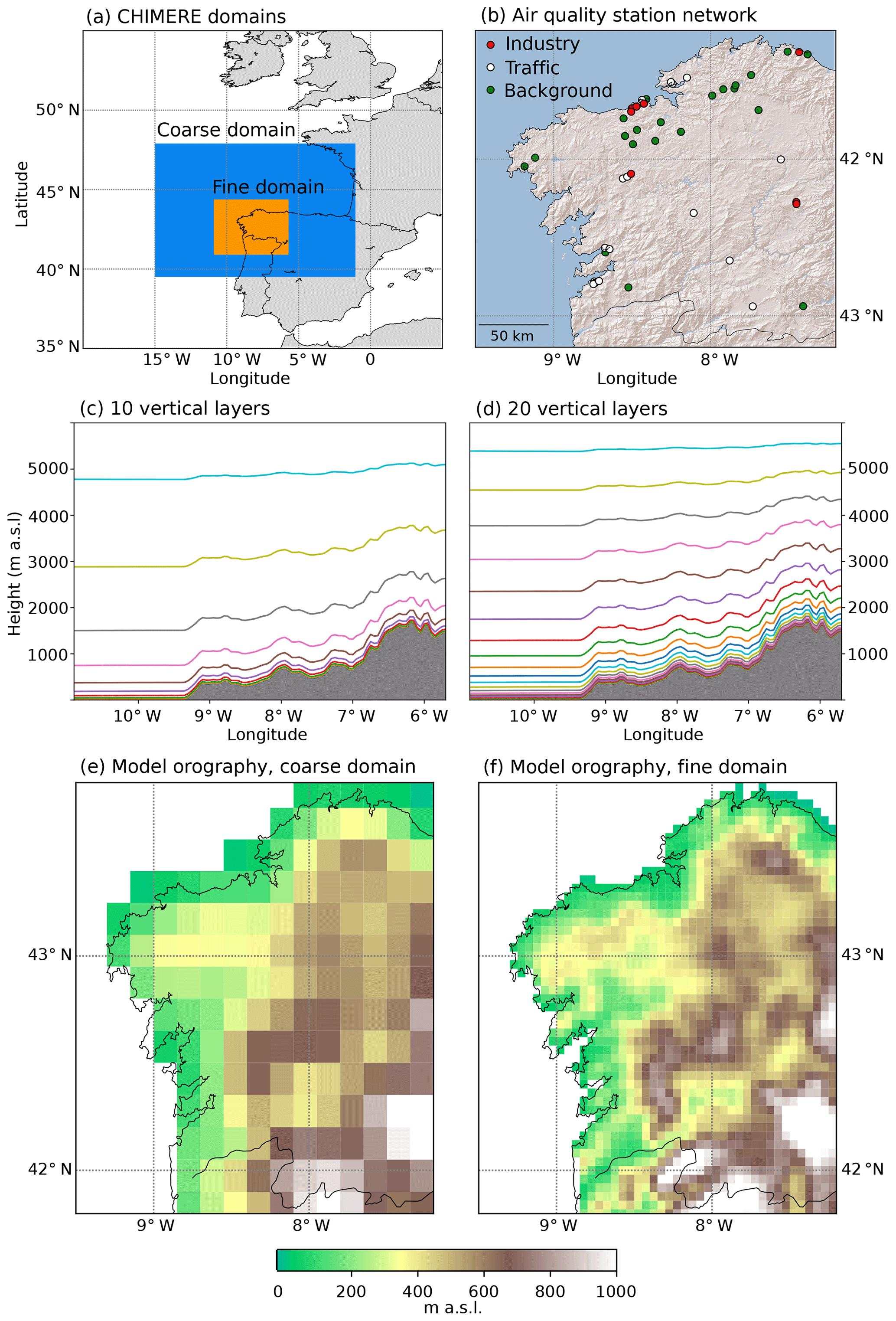
Figure 1 (a) Horizontal CHIMERE domains used for all sensitivity experiments. The fine domain (orange rectangle) is nested into the coarser one (blue rectangle). At the lateral boundary conditions of the coarse domain, CHIMERE is fed by time-varying C-IFS data. (b) The Galician air quality station network, grouped by the main pollution sources. (c) Height of the model layers in CHIMERE along 43^∘ N when using the 10-layer setup and the fine domain. Panel (d) is as (c) but for the 20-layer setup (e) model orography in meters above sea level (a.s.l.) for the coarse domain; panel (f) is as (e) but for the fine domain.

In Sect. 2, the applied data, model configurations and verification measures are described. Results are presented in Sect. 3, and a discussion and some general conclusions are provided in Sect. 4.

2 Data and methods

In this section, the meteorological input data and general characteristics of the CHIMERE experiments are depicted first (Sect. 2.1), followed by a description of the two applied emission inventories (Sect. 2.2) and individual model experiments (Sect. 2.3). The in situ station network used as a reference for verification is introduced in Sect. 2.4. The section closes with a description of the verification measures used to estimate CHIMERE's performance for the applied experiments (see Sect. 2.5).

2.1 Meteorological input and general characteristics of the CHIMERE experiments

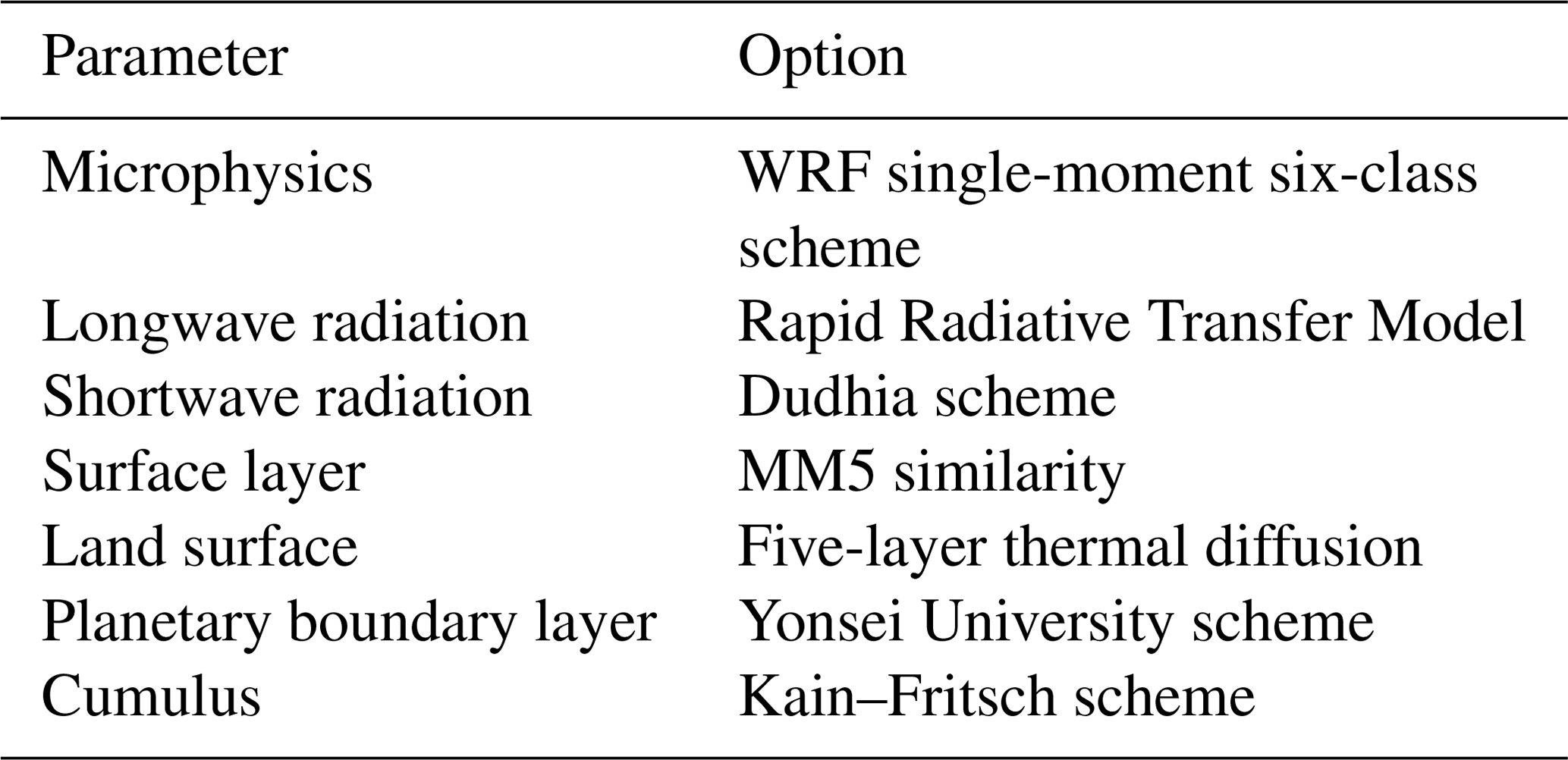
The meteorological input data for the CHIMERE experiments are provided by the Weather Research and Forecasting (WRF) model version 3.5 (Skamarock et al., 2008), driven by Global Forecast System (GFS) forecasts initialized at 00:00 UTC (Caplan et al., 1997). WRF is run on three domains: a continental-scale domain having a resolution of 36 km, followed by a regional domain covering southwestern Europe at a resolution of 12 km and, finally, a 4 km domain covering our study region, the northwestern Iberian Peninsula. For these domains, WRF is executed with a minimum time step of 216, 72 and 24 s and a maximum time step of 360, 180 and 60 s, respectively. All domains comprise 33 vertical layers with a model top at 10 hPa. A detailed overview of the WRF physics can be found in Table 1. In this configuration, WRF has been run for more than a decade at the meteorological office of the Galician government (MeteoGalicia) in order to provide real-time meteorological forecasts for the northwestern Iberian Peninsula. It is able to simulate orographic and coastal effects on the local weather reasonably well, which is illustrated in Supplement Fig. S1 for a typical summertime heat day (5 August 2018).

Table 1 WRF physics common to all sensitivity tests.

With this meteorological input, version 2017r4 of the CHIMERE model is run on two domains: a coarse domain having a horizontal resolution of $\mathrm{0.15}{}^{\circ }\times \mathrm{0.15}{}^{\circ }$ (longitude × latitude) and a fine domain nested into the former, having a resolution of $\mathrm{0.05}{}^{\circ }\times \mathrm{0.04}{}^{\circ }$ (see Fig. 1a). Note that the terms “coarse” and “fine” shall hereafter refer to the CHIMERE domains, not the WRF domains, if not otherwise stated. Biogenic emissions comprising volatile organic compounds (VOCs) and NO are from the MEGAN model version 2.04 (Guenther et al., 2006), and mineral dust emissions within the CHIMERE domains are calculated on the basis of the United States Geological Survey (USGS) land use dataset (Loveland et al., 2000). The Alfaro and Gomes (2001) saltation and sandblasting scheme, optimized by Menut et al. (2005), and the surface wind threshold described in Shao and Lu (2000) are used throughout all experiments. The effect of soil moisture on dust emissions (Fécan et al., 1999) is activated, and so are sea-salt emissions. Vertical advection is achieved by the upwind scheme and horizontal advection by the more complex van Leer (1979) scheme. Carbonaceous species as well as the interaction between aerosols and gases are taken into account by the model, and the number of Gauss–Seidel iterations is set to three because the model occasionally develops unrealistic waves with lower numbers. Wind speed reduction in urban areas (the so-called “urban correction”) is deactivated, and so is the resuspension process. A complete list of the internal CHIMERE parameters common to all sensitivity experiments is provided in Table 2. For a full description of these parameters, the interested reader is referred to the CHIMERE user manual available at http://www.lmd.polytechnique.fr/chimere.

Alfaro and Gomes (2001); Menut et al. (2005)Shao and Lu (2000)Fécan et al. (1999)Zhang et al. (2001)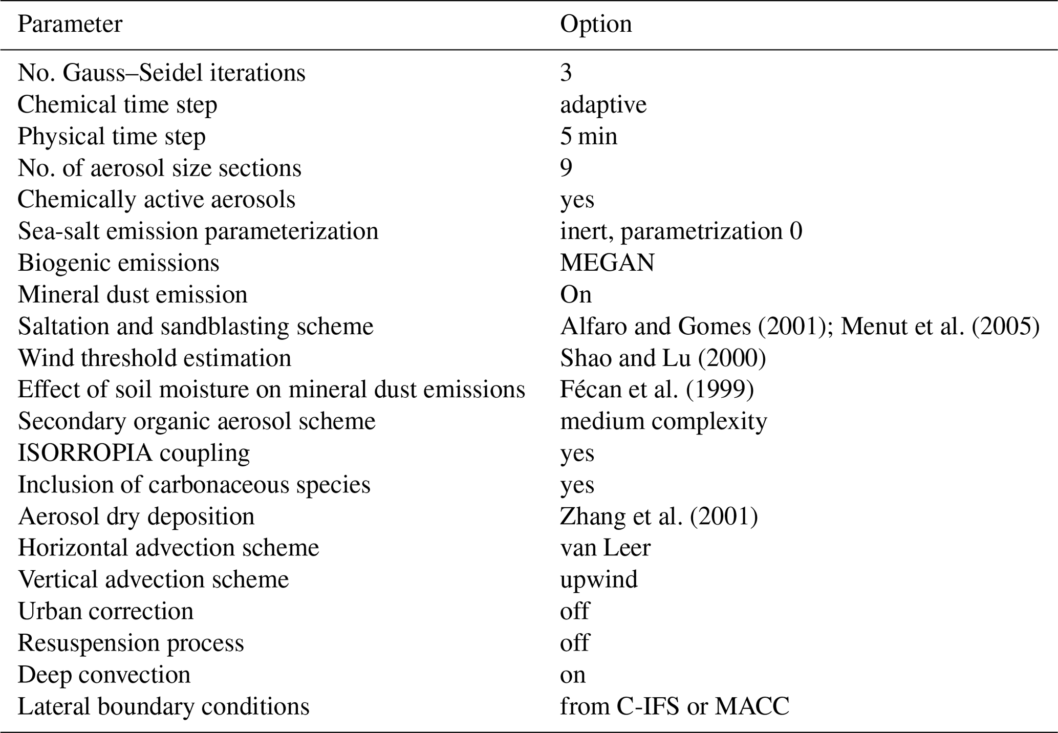

Table 2 CHIMERE parameters common to all sensitivity tests.

Along the lateral boundaries of the coarse domain, the concentrations of the chemical species required by CHIMERE are provided by 3-hourly forecasts of the ECMWF Composition Integrated Forecasting System (C-IFS) initialized at 00:00 UTC (Flemming et al., 2015). This global model comprises 60 vertical levels and has a horizontal resolution of ≈80 km. In the case that a chemical species required by CHIMERE is not provided by C-IFS, the monthly climatological mean values from the MACC reanalysis (Inness et al., 2013) are used instead. As an exception, sea-salt aerosols from MACC are applied although they are also available from C-IFS because the latter system was found to overestimate the corresponding concentrations in our study region. This bias is of minor importance for the summer season considered here but would lead to an overestimation of the PM concentrations in the other stormier seasons of the year. Similarly, the applied dust aerosols from C-IFS are scaled by a factor of 0.6 in order to compensate for the positive bias observed during the two Saharan dust events occurring in the time period considered here. For all other chemical species from C-IFS, a scaling factor of 1 (i.e., no scaling) is used. The fact that the chemical and physical boundary conditions for our CHIMERE forecasts come from different prediction systems is assumed to be of minor importance for the short lead times analyzed here (27 h from initialization at the utmost).

To eliminate unwanted effects related to the spin-up, the daily WRF forecasts are initialized with the digital filtering initialization (DFI) technique (Skamarock et al., 2008), and the first 3 h of integration are not used as meteorological input to CHIMERE. Consequently, CHIMERE is initialized at 03:00 UTC using initial conditions from the model execution of the previous day and is then integrated until 03:00 UTC of the following day to complete one forecast day. This procedure is repeated for each day from 20 June 2018 to 21 August 2018, and the resulting model output is then concatenated to form time series covering the entire time period. The verification against surface observations as described in Sect. 2.5 begins on 21 June 03:00 UTC, so CHIMERE is permitted to spin-up during the first 24 h of the integration.

2.2 Anthropogenic emission inventories, land use databases and post-processing

To assess CHIMERE's combined sensitivity to changes in the anthropogenic emissions, downscaling strategy and land use database, two distinct inventories and post-processing techniques were selected: the EMEP dataset for the year 2017 on the one hand (EMEP/CEIP, 2019) and the HTAP v2.2 dataset for the year 2010 on the other (Janssens-Maenhout et al., 2015), both provided on a regular $\mathrm{0.1}{}^{\circ }\times \mathrm{0.1}{}^{\circ }$ latitude–longitude grid. To disaggregate the raw data from these inventories, the publicly available program emiSURF shipped with the CHIMERE source code was used (Mailler et al., 2017), which was modified here to process EMEP data on the recently published $\mathrm{0.1}{}^{\circ }\times \mathrm{0.1}{}^{\circ }$ grid. Spatial disaggregation is achieved by downscaling the emissions from their native grid to an auxiliary high-resolution grid at 1 km, followed by an upscaling to the two target domains displayed in Fig. 1a. In this downscaling step, different proxies can be used to redistribute the raw emission data on the subgrid scale, among which land use categories are the standard option of the emiSURF program.

To downscale the raw HTAP v2.2 emissions, land use categories from the USGS dataset were used as the only proxy except for the “population downscaling” experiment, for which population density was used as an additional proxy (Gallego, 2010). The latter type of downscaling affects the NO₂ and particulate matter emissions from SNAP sector 2, originating mainly from domestic fuel burning (Mailler et al., 2017).

To spatially regrid the EMEP inventory, road traffic density and the locations of large point sources were used in addition to population density and land use categories, the latter provided by the GlobCover dataset in this case (Bicheron et al., 2011). The road traffic proxy affects the magnitude and allocation of the NO₂ emissions caused by this kind of activity, whereas the locations of large point sources are used to reallocate the corresponding emissions on the subgrid scale. The temporal disaggregation of the raw anthropogenic emission data to the timescale required by CHIMERE was accomplished by using seasonal, weekly and hourly profiles for each pollutant and activity sector, which are implemented in the standard CHIMERE preprocessors (Menut et al., 2012; Mailler et al., 2017).

The above explained large differences between the spatial downscaling procedures of the two emission inventories were applied intentionally to assess CHIMERE's performance for the use of (1) an up-to-date and sophistically downscaled inventory (EMEP) vs. (2) an older inventory downscaled with basic parameters (HTAP v2.2). For ease of understanding, these will hereafter be referred to as emission configuration 1 and emission configuration 2, respectively.

2.3 Specific configuration of the sensitivity tests

To explore the influence of vertical resolution on model performance, 10-layer experiments are compared to 20-layer experiments, the lowermost layer being located at 999 hPa and the uppermost at 500 hPa in all cases (see Fig. 1c and d). Thus, an increase in vertical resolution refers to a refinement in the lower to middle troposphere. An extension of the model top to, e.g., 200 hPa has been proposed in previous studies since some dust intrusions may extend to pressure levels above 500 hPa (Bessagnet et al., 2017). However, by the design of our experiments, most of the dust intrusion trajectory is simulated by the global atmospheric composition model, providing the lateral boundary conditions (C-IFS) rather than internally simulated by CHIMERE, and therefore elevating the model top is assumed to be of minor importance here.

The effect of an increase in horizontal resolution is tested by comparing the model output obtained with the coarse-resolution domain with that of the fine-resolution domain nested therein (see Fig. 1a, e and f). In all but one fine-resolution experiment (the “coarse meteorology” experiment defined below) the horizontal resolution increase is undertaken in both CHIMERE and WRF, meaning that the combined effect is assessed.

Version 2017r4 of the CHIMERE model offers the possibility to use three distinct “chemical mechanisms” describing the gas-phase chemistry considered by CHIMERE. The “full Melchior” mechanism consists of 300 reactions and 80 gaseous species and is the most complete but also the most computationally demanding of the three. This is why a reduced version with 120 reactions and 40 species, the so-called “reduced Melchior” or “Melchior 2” mechanism, is available as well. From version 2016a onwards, the SAPRC mechanism is implemented as the third mechanism (Carter, 2010), offering a chlorine chemistry not considered in either of the two Melchior mechanisms (Mailler et al., 2017). With 72 gaseous species and 218 chemical reactions, SAPRC's complexity and computational costs are somewhat lower than for full Melchior but superior to reduced Melchior. For the European summer 2015, reduced Melchior and SAPRC are compared in Menut et al. (2013b), who found large differences in the composition of organic nitrogen between the two, which could potentially influence the spatial distribution of ozone production. They also found that the systematic overestimation of surface ozone reported in many CHIMERE studies is slightly less of a problem when using SAPRC. In the present study, however, the full version of the Melchior mechanism is applied instead of the reduced one, meaning that the aforementioned findings might not hold here.

All the aforementioned model configurations, comprising two horizontal and two vertical resolution setups as well as two chemical mechanisms, are run separately with emissions configuration 1 and 2 as defined in Sect. 2.2.

Finally, three additional sensitivity tests are applied with constant anthropogenic emissions (HTAP), horizontal and vertical resolution (fine mesh, 20 layers), chemistry mechanism (full Melchior), and land use database (USGS). First, the effects of using the population proxy for downscaling the raw HTAP emissions are explored in what is called the population downscaling experiment (FM20H-P) hereafter. Then, the fine horizontal CHIMERE mesh is run with the coarse WRF mesh in the coarse meteorology experiment (FM20H-C) in order to see whether low-resolution meteorological input deteriorates CHIMERE's performance. Finally, the effects of missing biogenic emissions are explored by intentionally turning them off in the “no biogenic emissions” experiment (FM20H-N).

For further reading, it is helpful to understand the rationale behind the abbreviations used for the distinct experiments. The first letter of a given abbreviation refers to the horizontal resolution of the CHIMERE mesh (C: coarse or F: fine), the second letter to the applied chemical mechanism (M: Melchior or S: SAPRC) and the following number to the vertical model levels used in the experiment (10 or 20). The third letter then points to the applied anthropogenic emission configuration (E: EMEP or H: HTAP) and the optional fourth letter separated by a hyphen to one of the three specific experiments described above (P: population downscaling, C: coarse meteorology, N: no biogenic emissions).

Table 3 Overview of the applied sensitivity tests. C: coarse horizontal resolution, F: fine horizontal resolution, 10: number of vertical layers, S: SAPRC, M: full Melchior, E: EMEP, H: HTAP, P: population downscaling, C: coarse meteorology, N: no biogenic emissions, lu: land use, popul: population, lsp: emission allocation according to large point sources; runtime is in seconds for a typical summertime heat day (5 August 2018). Experiments marked with an asterisk are mapped in Figs. 2, 3, 6 and 7.

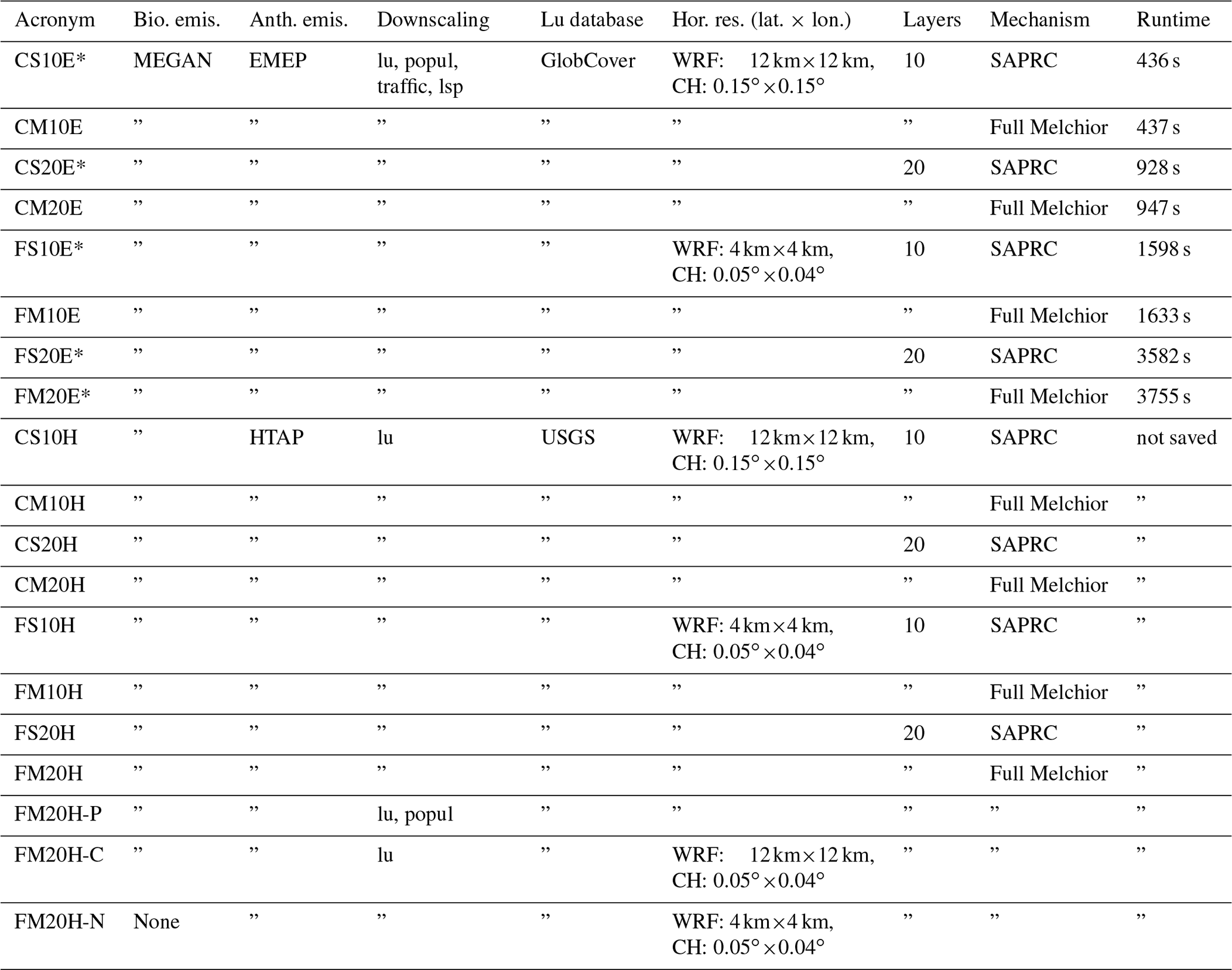
An overview of all applied sensitivity tests is provided in Table 3. In the last column, the computational costs for a typical summertime heat day (5 August 2018) are listed for the emission configuration 1 experiments. The runtimes of the respective configuration 2 experiments are in very close agreement (e.g., for CS10H and CS10E) but cannot be exactly stated since they were unfortunately not saved.

2.4 The air quality monitoring network in northwestern Spain (Galicia)

The Galician air quality monitoring network comprises a total of 46 stations, which, as a function of the main pollution source or the lack thereof, can be grouped into background, industrial and traffic sites (see Fig. 1b). Currently, 14 stations are directly maintained by the Galician regional government (Xunta de Galicia). The remaining 32 stations are maintained by industrial companies supervised by the government in order to ensure the same measurement standards specified in the national UNE-EN norm.

The quality control of the corresponding data is accomplished manually by trained technical staff of the regional government, i.e., is centralized in one institution. First, outlier values are detected by comparing a suspicious value to the typical time series behavior at the considered site and at the surrounding sites. Once the outlier is detected, its validity is determined taking into account inter-variable relationships, potential power breakdowns, calibration errors, damages and changes in the topographic features surrounding the station. This way, a quality-controlled observational dataset has been developed which, at some locations, is now nearly a decade long. This dataset serves as a reference for model verification.

2.5 Applied verification measures

Here, the temporal agreement between the modeled and observed time series is measured in terms of the Pearson correlation coefficient (R), the percentage bias (see Eq. 1) and the standard deviation ratio (see Eq. 2):

$$\begin{array}{}\text{(1)}& {\displaystyle }& {\displaystyle }\text{BIAS}={\displaystyle \frac{\stackrel{\mathrm{‾}}{m}-\stackrel{\mathrm{‾}}{o}}{\stackrel{\mathrm{‾}}{o}}}\times \mathrm{100},\text{(2)}& {\displaystyle }& {\displaystyle }\text{RATIO}={\displaystyle \frac{{\mathit{\sigma }}_{\mathrm{m}}}{{\mathit{\sigma }}_{\mathrm{o}}}},\end{array}$$

where $\stackrel{\mathrm{‾}}{m}$, $\stackrel{\mathrm{‾}}{o}$, σ_m and σ_o are the modeled and observed values for the temporal mean and standard deviation, respectively.

Note that the chosen verification measures are complementary to each other since they cover different time series aspects. Namely, BIAS and RATIO measure the model's capacity to reproduce the observed temporal mean and dispersion, whereas R looks at the similarity in day-to-day variability irrespective of errors in the mean and dispersion. The perfect scores for BIAS, RATIO and R are 0, 1 and 1, respectively.

In addition, the mean absolute error (MAE) is a good measure of overall performance and is applied here as a skill score (mean absolute error skill score, MAESS), i.e., as percentage deviation from the error of a reference experiment:

$$\begin{array}{}\text{(3)}& {\displaystyle }{\displaystyle }\text{MAESS}=\left(\mathrm{1}-{\displaystyle \frac{{\text{MAE}}_i}{{\text{MAE}}_{\text{ref}}}}\right)\times \mathrm{100},\end{array}$$

where MAE_i is the error a specific experiment i and MAE_ref the error of the experiment CS10E, used as a reference throughout the present study since it is the computationally least expensive experiment (see Table 3). Positive values indicate performance gains and negative values performances losses with respect to the reference (Jolliffe and Stephenson, 2012). These verification measures are applied to hourly mean observations and hourly model data as provided by CHIMERE as well as to the daily minimum and maximum values obtained from the former. All verification results are for the lowermost model layer whose upper limit is located at 999 hPa, i.e., roughly 10 m above the ground.

The aforementioned temporal verification scores are calculated separately for each station exceeding the 80 % threshold of valid values and are then visualized either by overlay maps or box plots. The center line of each box plot refers to the median value of the group of pointwise temporal verification results and the box to the interquartile range (IQR) of this group. The whiskers extend from the 25th percentile minus 1.5 × IQR at the lower end to the 75th percentile plus 1.5 × IQR at the upper end. Outlier verification results beyond these limits are not shown since their inclusion would expand the scale of the figures and thus hamper their interpretability.

Apart from these temporal verification scores, the spatial bias (SBIAS, S: spatial), correlation coefficient (SR), standard deviation ratio (SRATIO) and mean absolute error (SMAE) were calculated on the pointwise temporal mean values in order to assess whether the spatial statistics of the average pollutant concentrations are captured by the model. Likewise, the same scores have been applied on the pointwise temporal standard deviation values to assess whether the model reproduces the spatial statistics of temporal variability.

3 Results

3.1 Maximum values

3.1.1 Temporal mean and standard deviation

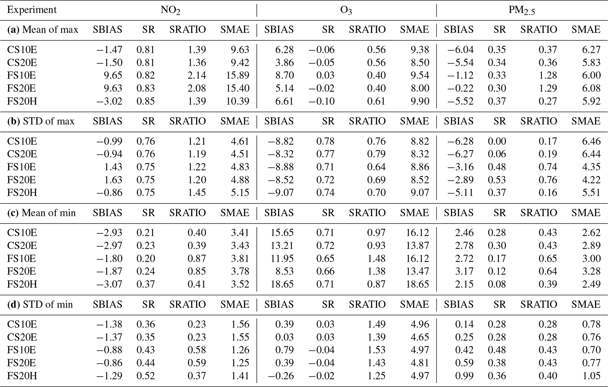
Figure 2 shows the temporal mean values of the daily maximum concentrations seen in observations (the dots) plotted on the respective model value (the underlying pattern) for the four experiments driven with emission configuration 1 and the chemical mechanism SAPRC (CS10E, CS20E, FS10E and FS20E, rows 1–4). Rows are ordered so that the first pair refers to the coarse horizontal mesh and the second pair to the fine one. Further, the 10- and 20-vertical-layer experiments are placed on top of each other to assess the effects of an increase in vertical resolution. In the fifth row, the fourth experiment (fine horizontal resolution, 20 layers) is replicated with emission configuration 2 to show the effects of a combined change in the choice of the anthropogenic emission inventory (from EMEP to HTAP), downscaling technique (from land use, population and traffic downscaling to land use downscaling only) and land use database (from GlobCover to USGS). The spatial bias (SBIAS; µg m⁻³), correlation coefficient (SR), standard deviation ratio (SRATIO = σ_model∕σ_obs) and mean absolute error (SMAE) of the modeled vs. observed temporal mean values for these experiments are provided in Table 4a.

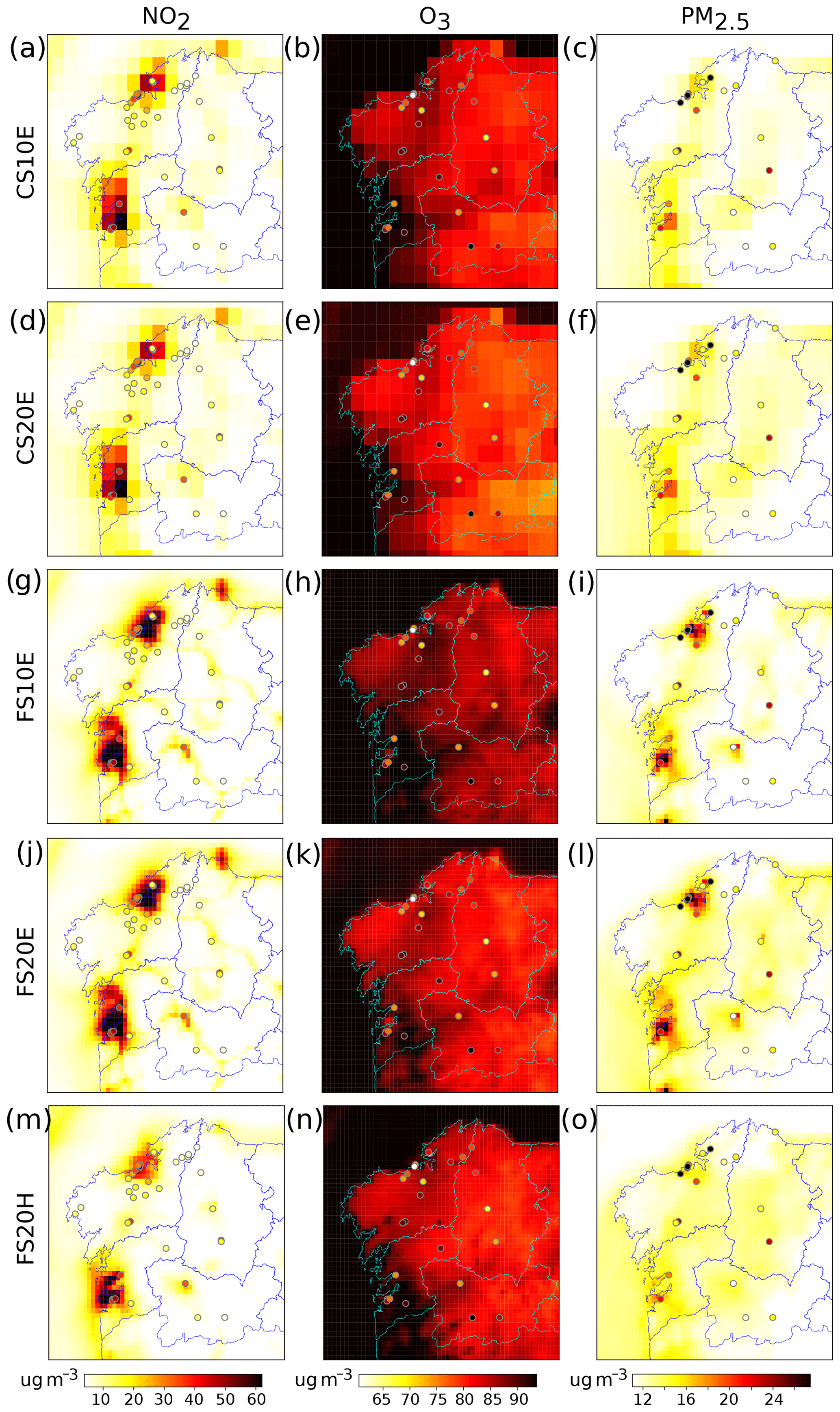
Figure 2 Observed (dots) vs. modeled (underlying pattern) temporal mean values for the daily maximum concentrations of NO₂, O₃ and PM_2.5, as well as the five experiments marked with an asterisk in Table 3, all run with the SAPRC mechanism. The spatial verification results for each panel are provided in Table 4a.

Table 4 Spatial verification results for Figs. 2, 3, 6 and 7 are displayed in the table sections a, b, c and d, respectively. Shown is the spatial mean difference (bias; µg m⁻³), correlation coefficient, standard deviation ratio (modeled ∕ observed) and mean absolute error (µg m⁻³) calculated upon the modeled and observed temporal mean or standard deviation values at the stations shown in these figures. SBIAS: spatial bias, SR: spatial correlation coefficient, SRATIO: spatial standard deviation ratio, SMAE: spatial mean absolute error, mean: results for the pointwise temporal mean values, STD: results for the pointwise temporal standard deviation values, max: results for daily maximum concentrations, min: results for daily minimum concentrations.

An increase in horizontal resolution improves the model's performance for PM_2.5 by reducing SBIAS and by bringing SRATIO closer to unity. For NO₂ and O₃, however, model performance either does not improve or clearly deteriorates. Most notably, SBIAS increases for both species and SRATIO does so for NO₂, eventually exceeding a value of 2, which means that the spatial dispersion of the modeled mean NO₂ maxima is more than twice the observed one. As will be shown below (see Sect. 3.1.2), these error increases are likely associated with the population downscaling technique used to disaggregate the raw EMEP emissions.

An increase in vertical resolution reduces SBIAS by up to 2. 4µg m⁻³ (i.e., 40 %) for the mean O₃ values and by up to 0.9 µg m⁻³ (i.e., 80 %) for the mean PM_2.5 values. For the latter pollutant, vertical refinement is much more efficient when using the fine horizontal mesh, in which case SBIAS is clearly improved.

For the fine horizontal mesh and 20 vertical layers, a switch to emission configuration 2 (i.e., from FS20E to FS20H; compare rows 4 and 5) translates into an improvement of SRATIO for NO₂ and O₃ but to a worsening for PM_2.5. Also, results for FS20H are in closer agreement with CS20E than with FS20E, which points to the fact that the temporal mean daily maximum concentrations are more sensitive to the particular setup of the downscaling technique than to differences in the raw emission inventories.

In all considered experiments, the simulated mean O₃ concentrations are considerably higher over the sea than over land, which is in line with Terrenoire et al. (2015) and might be explained by reduced dry deposition and nighttime destruction by NO₂ over the sea resulting from a reduced surface roughness and NO₂ availability there (Davies et al., 1992; O'Hare and Wilby, 1995). Since this land–sea contrast is not seen in observations, the SR values for all experiments are essentially zero. This can be explained by either the lack of offshore background observations (note that all available coastal sites are affected by urban pollution) or by the fact that the reduced ozone destruction over the sea is less pronounced in the model than in the real world, translating into a positive bias there.

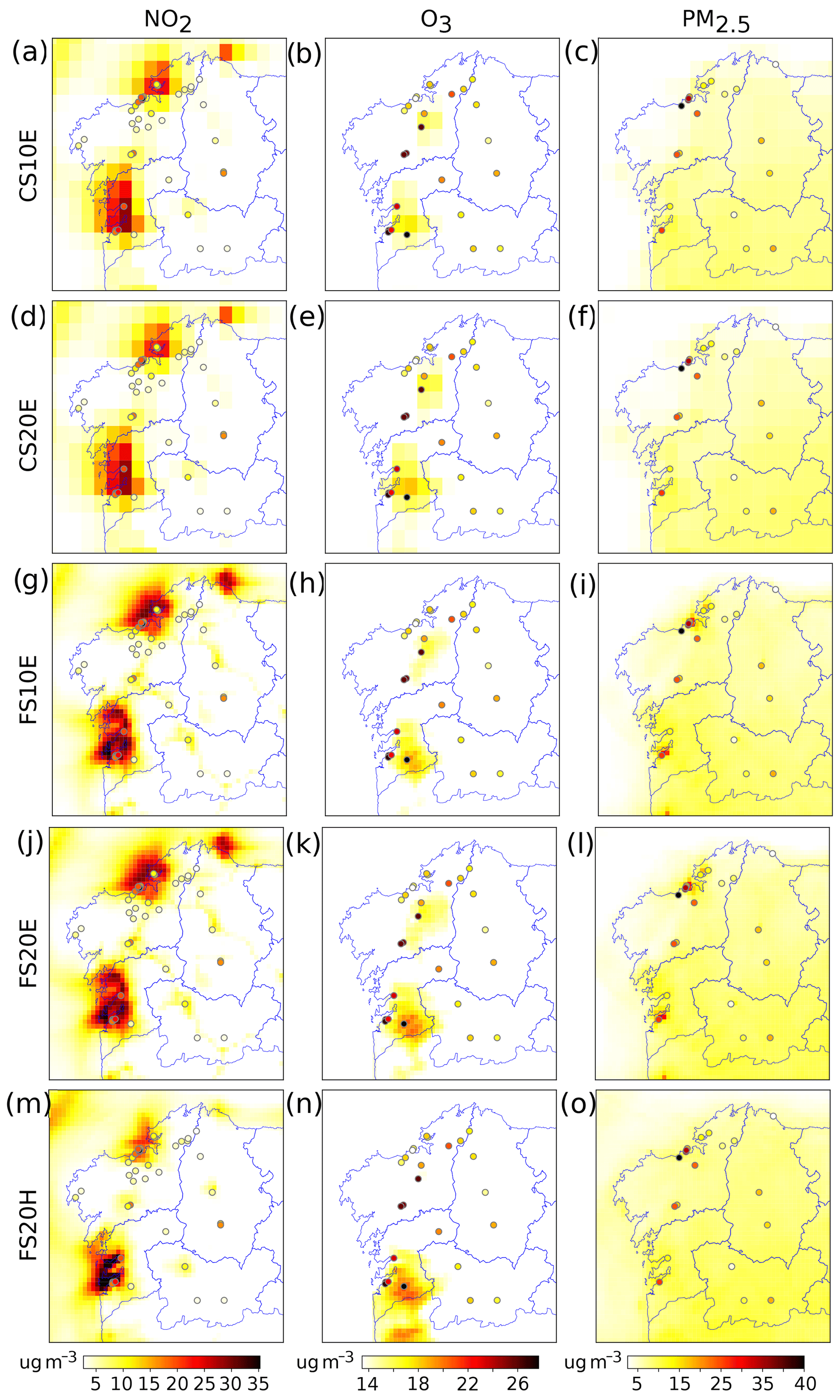
Figure 3 Observed (dots) vs. modeled (underlying pattern) temporal standard deviation values for the daily maximum concentrations of NO₂, O₃ and PM_2.5, as well as the five experiments marked with an asterisk in Table 3), all run with the SAPRC mechanism. The spatial verification results for each panel are provided in Table 4b.

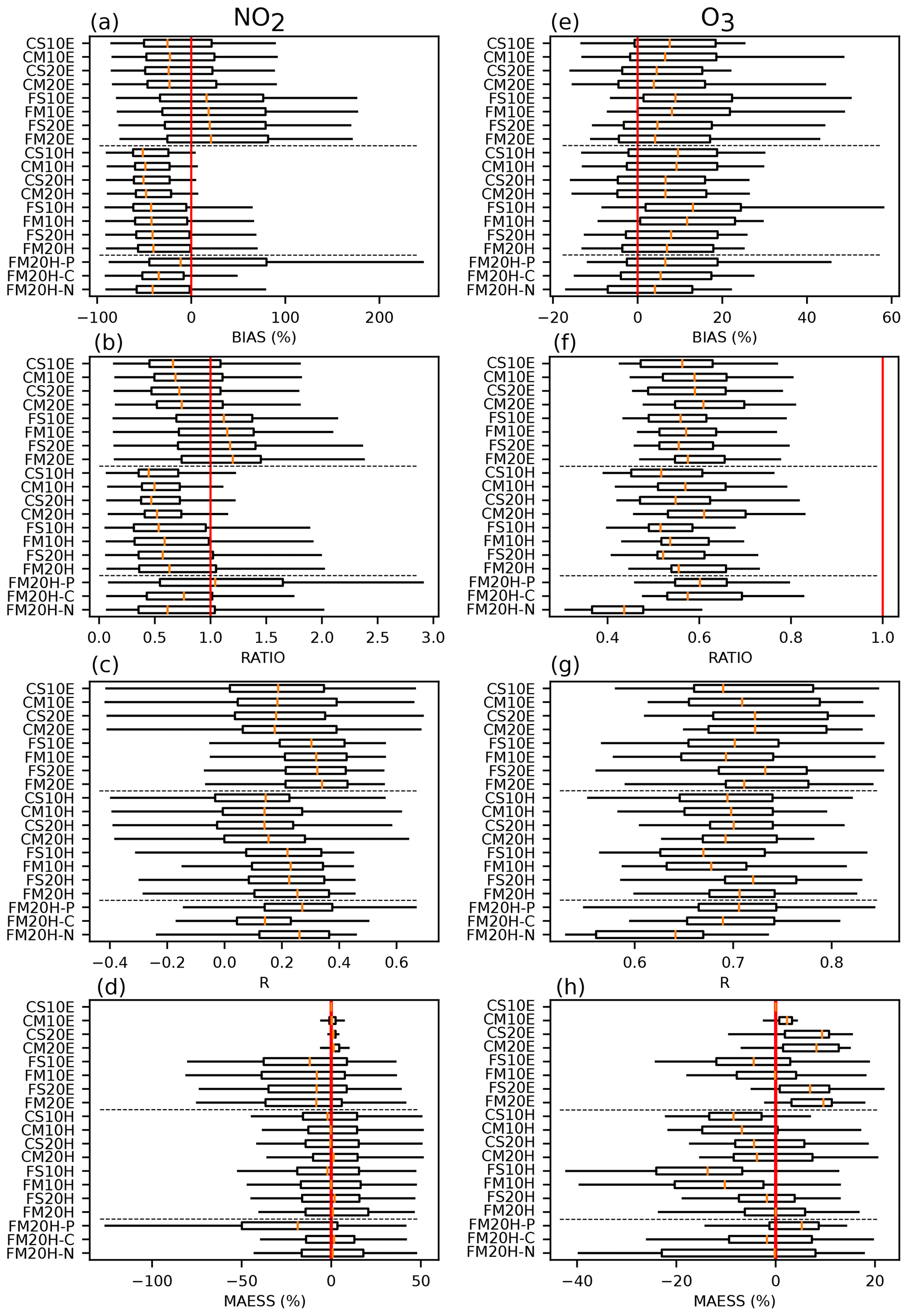
Figure 4 Temporal verification results for daily near-surface maximum NO₂ (a–d) and O₃ (e–h). (a, e) Percentage bias (BIAS), (b, f) Pearson correlation coefficient (R), (c, g) ratio of standard deviation (RATIO), (d, h) mean absolute error skill score (MAESS) with reference to the base experiment CS10E. Box plots are calculated upon the pointwise verification results at all available stations. Experiments are explained and grouped as in Table 3.

Figure 4 shows the temporal standard deviation of the daily maximum concentrations as seen in observations vs. those seen in the model, i.e., the model's capability to reproduce the observed temporal variability. The respective spatial verification results are provided by Table 4b. In general, CHIMERE is plagued by underdispersion, i.e., tends to underestimate the temporal variability of the daily maximum concentrations (SBIAS is negative). An increase in horizontal resolution alleviates this problem for PM_2.5 and even leads to overdispersion for NO₂ (i.e., to a positive SBIAS), but it does not noticeably alter the results for O₃. For PM_2.5, SR is much improved when considering the fine horizontal mesh. Contrary to the findings for the temporal mean, temporal variability is more sensitive to a horizontal resolution increase than to a vertical resolution increase. Except for PM_2.5, the impact of a switch in the emission configuration is less pronounced for the temporal standard deviation than for the aforementioned temporal mean (compare rows 4 and 5 in Figs. 3 and 4)

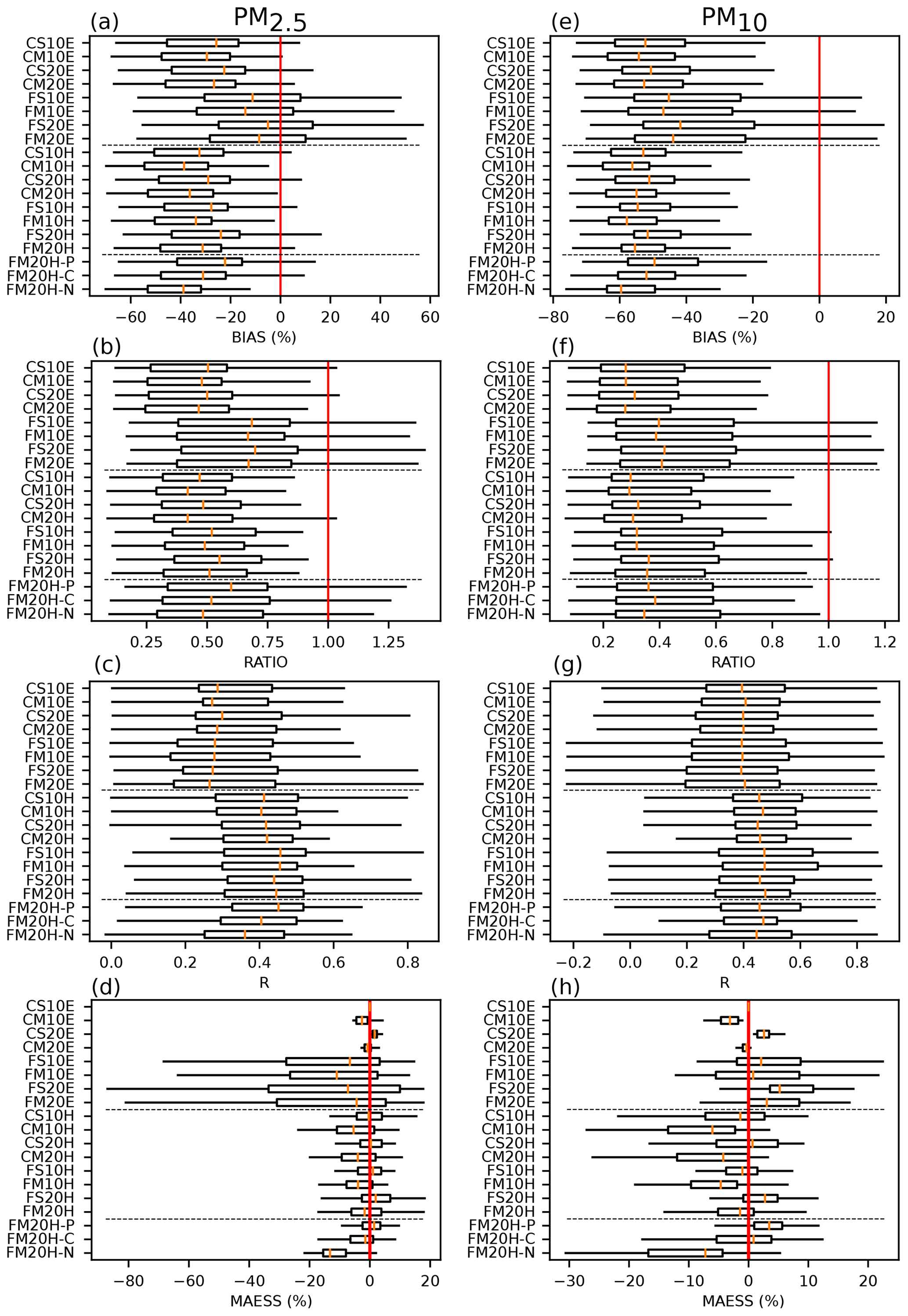
Figure 5 Temporal verification results for daily near-surface maximum PM_2.5 (a–d) and PM₁₀ (e–h). (a, e) Percentage bias (BIAS), (b, f) Pearson correlation coefficient (R), (c, g) ratio of standard deviation (RATIO), (d, h) mean absolute error skill score (MAESS) with reference to the base experiment CS10E. Box plots are calculated upon the pointwise verification results at all available stations. Experiments are explained and grouped as in Table 3.

3.1.2 Full temporal verification

Figure 5 shows the verification results of all applied experiments as ordered in Table 3 for the daily maximum NO₂ and O₃ concentrations. The perfect score for a given verification measure is indicated by a red vertical line. As can be seen from the figure, the NO₂ concentrations are generally underestimated by the model, except for the four emission configuration 1 experiments run at a high horizontal resolution (see Fig. 4a). Emission configuration 2 is plagued by larger median biases (see vertical orange lines within the boxes) than configuration 1 but has the advantage of a lower spatial spread in the results (see width of the boxes and whiskers). When applying a high horizontal resolution, this bias is reduced on average but the aforementioned spread is largely increased. While the effects of a vertical resolution increase and/or switch in the applied chemical mechanism are negligible, the effect of population downscaling is considerable. Namely, the smallest median bias but largest spatial spread among all experiments are yielded if the raw HTAP emissions are disaggregated this way (see FM20H-P in Fig. 4a).

The structure of the verification results for the standard deviation ratio (see Eq. 2 in Sect. 2.5) is in very close agreement with the structure found for the percentage bias, and virtually identical lessons are learned (compare panel b with a in Fig. 4).

The model's capability to reproduce the temporal sequence of the observed anomalies, here measured with the Pearson correlation coefficient (R), is most improved by an increase in the horizontal resolution (see Fig. 4c). Emission configuration 1 yields systematically better results than configuration 2 (compare experiments ending in E with those ending in H in Fig. 4c). As opposed to the bias, the spatial spread of the correlation coefficient is larger for the coarse horizontal resolution than for the fine one, particularly if emission configuration 1 is used (compare the spread of the C-type experiments in Fig. 4c). The full Melchior mechanism yields slightly better correlation coefficients than SAPRC, and so does the use of 20 instead of 10 vertical layers.

As indicated by Fig. 4d, the MAESS of the reference experiment CS10E is improved only by the CM20E experiment, meaning that the use of 20 vertical layers together with the full Melchior mechanism is sufficient to achieve optimal results for this measure. A horizontal resolution increase is not necessary and is actually counterproductive if emission configuration 1 is used.

The inclusion of the population proxy in the downscaling procedure of the HTAP inventory leads to a sharp decrease in the spatial median MAESS and to the largest spatial spread among all experiments (see FM20H-P in Fig. 4d). In comparison, the use of coarse meteorological input data or removal of biogenic emissions has much smaller effects on the model's performance (compare FM20H-C and FM20H-N with FM20H in Fig. 4d)

As shown in Fig. 4e and f, CHIMERE overestimates the temporal mean and underestimates the temporal variability of the daily maximum O₃ concentrations. The effect of the performance factors is similar for each of the four applied verification measures. In general, the respective error is improved by a vertical resolution increase and by applying full Melchior instead of SAPRC, but it is deteriorated or not improved when the horizontal resolution is increased. As an exception, SAPRC generally yields better correlation coefficients if the fine horizontal mesh is used (see Fig. 4g). Contrary to Menut et al. (2013b), average O₃ concentrations are larger for the SAPRC mechanism than for full Melchior. When considering MAESS, the emission configuration is the most influential factor on model performance, with configuration 1 clearly outperforming configuration 2 (see Fig. 4h). As was the case for maximum NO₂, 20 vertical layers yield better results than 10 layers, and for the use of emission configuration 1, the 20-layer setup performs nearly as well for the coarse horizontal mesh as for the fine one, meaning that the former is again preferable in the case that computational resources are limited (see last column in Table 3).

The full temporal verification results for the daily maximum PM_2.5 and PM₁₀ concentrations are displayed in Fig. 5. As shown in panels (a), (b), (e) and (f), CHIMERE generally underestimates the temporal mean value and variability for both particle size fractions. The most important performance factor is the emission configuration, yielding smaller bias values with configuration 1 (see Fig. 5a and e) and better correlation coefficients with configuration 2, particularly for the fine particles (Fig. 5c and g). The effects of a horizontal resolution increase depend on the considered emission configuration and particle size fraction. Namely, configuration 1 improves the bias and standard deviation ratio for both size fractions (Fig. 5a, b, e, f) but has no effect on the correlation coefficient (Fig. 5c and g). Configuration 2, in turn, improves the correlation coefficient of the fine particles (Fig. 5c) but does not affect the bias or the standard deviation ratio for any of the two particle size fractions (5a–b and e–f). A vertical resolution increase improves the bias for both particle sizes and, if a fine horizontal mesh is applied in addition, also the standard deviation ratio for the fine particles. The correlation coefficient, however, cannot be improved by a horizontal resolution increase and even deteriorates for some experiments (Fig. 5c and g). Regarding overall performance as measured by the MAESS (5d and h), SAPRC yields better results than full Melchior for nearly all experiments and both size fractions. The most robust skill increases are again obtained with 20 vertical layers, the coarse horizontal resolution, the SAPRC mechanism and emission configuration 1 (CS20E). Although the performance increase at individual stations may be much larger for other experiments, CS20E yields positive MAESS values at all stations and for both particle sizes. If the fine horizontal resolution is used (FS20E), the average performance improves for PM₁₀ but deteriorates for PM_2.5. FS20H and FM20H-P perform equally as well as CS20E on average but are characterized by a larger spatial spread in the results.

The population downscaling experiment outperforms its base experiment or is comparable to it for both particle sizes (compare FM20H-P with FM20H in all panels in Fig. 5). Using coarse-resolution meteorological input does not noticeably affect the results, except for a clear decrease in correlation for the fine particles (compare FM20H-C with FM20H in Fig. 5c). A lack of biogenic emissions, however, largely enhances the bias (compare FM20H-N with FM20H in Fig. 5a and e), reduces the correlation (Fig. 5c and g) and worsens the overall performance as measured by the MAESS (Fig. 5d and h).

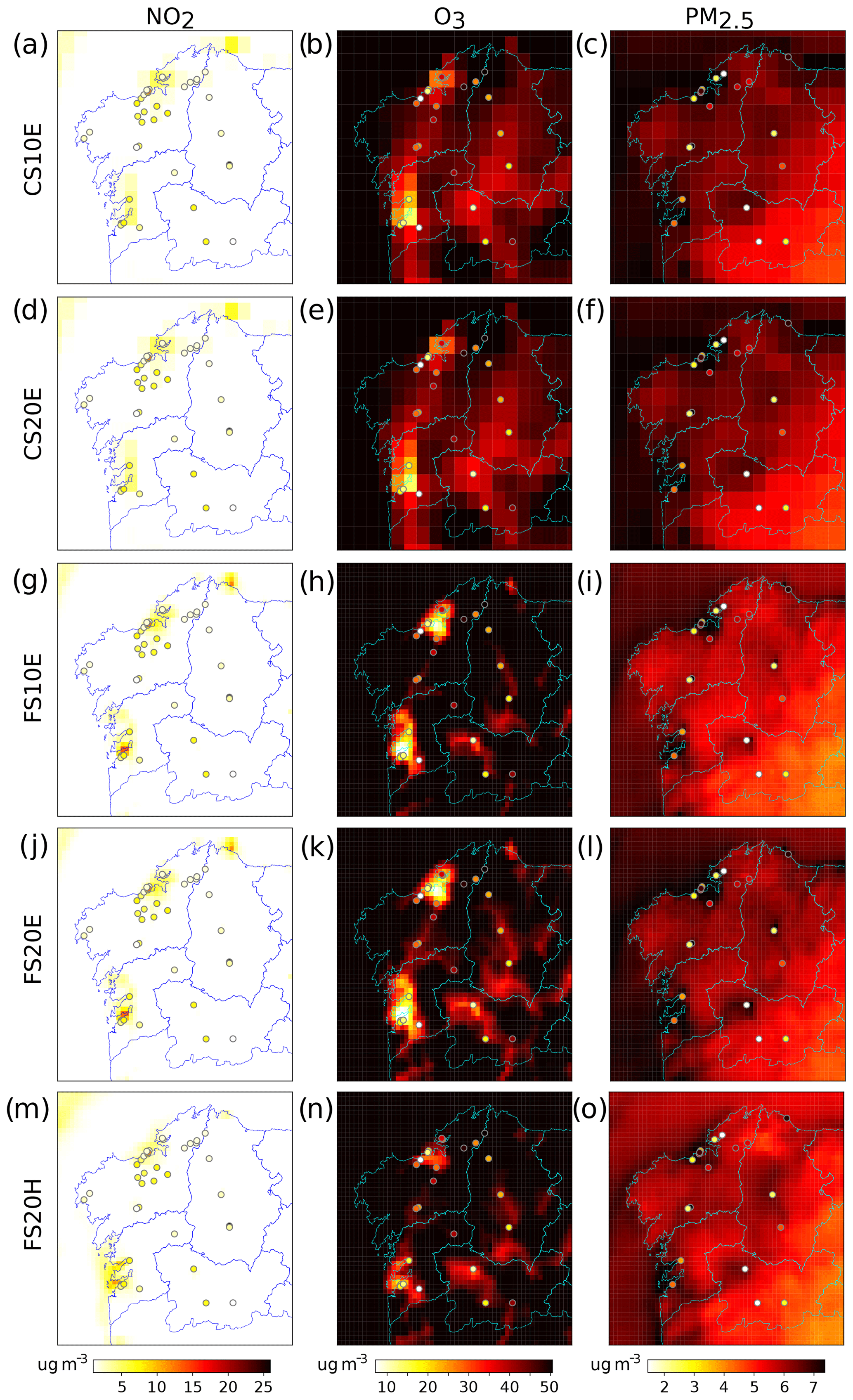
Figure 6 Observed (dots) vs. modeled (underlying pattern) temporal mean values for the daily minimum concentrations of NO₂, O₃ and PM_2.5, as well as for the five experiments marked with in asterisk in Table 3, all run with the SAPRC mechanism. The spatial verification results for each panel are provided in Table 4c.

3.2 Minimum values

3.2.1 Temporal mean and standard deviation

Figure 6 shows the temporal mean values of the daily minimum NO₂, O₃ and PM_2.5 concentrations seen in observations (the dots) plotted on the respective model value (the underlying pattern) for the five experiments assessed in Sect. 3.1.1. The respective spatial verification results are provided in Table 4c. For NO₂ (Fig. 6, column 1), the model underestimates the temporal mean concentrations on average (SBIAS<0) and underestimates their spatial dispersion (SRATIO<1). The spatial pattern of the observed mean values is not well reproduced either (SR<0.25 in Fig. 6a, d, g, and j). While the former two error types can be improved by augmenting the horizontal resolution (compare panels a and d with panels g and j in Fig. 6), the latter one can be reduced by using emission configuration 2 (compare panel j with m). Similar to the results for the maxima, using 20 instead of 10 vertical layers does not noticeably improve the result for the NO₂ minima either (compare Fig. 6a with d and g with j).

As for the maxima, the average minimum O₃ concentrations (Fig. 6, column 2) are overestimated by the model (SBIAS>0). However, the spatial pattern of the observed values is generally well reproduced (RS≥0.65), and so is the spatial dispersion if the coarse horizontal mesh is used (SRATIO≈1). Using the fine horizontal mesh on the one hand reduces the bias but, on the other, inflates the spatial dispersion (SRATIO>1, compare Fig. 6b with h and e with k). Results are improved when 20 instead of 10 vertical layers are used in combination with the fine horizontal mesh (compare panels h and k), and the bias largely increases when emission configuration 1 is applied (compare panels k and n).

The temporal mean daily PM_2.5 minima (Fig. 6, column 3) are on average overestimated by the model (SBIAS>0), their spatial dispersion is underestimated (SRATIO well below unity) and their spatial pattern not well reproduced (low values for SR). A horizontal resolution increase improves the spatial dispersion but deteriorates the spatial pattern and increases the bias, meaning that the negative effects prevail for this factor (compare Fig. 6 c with i and f with l). A vertical resolution increase generally has little effect on the model's performance unless the horizontal resolution is also increased, in which case the bias increases for PM_2.5 (compare c with with f and i with l). As for the maxima, results for FS20H are generally more similar to CS20E than to FS20E.

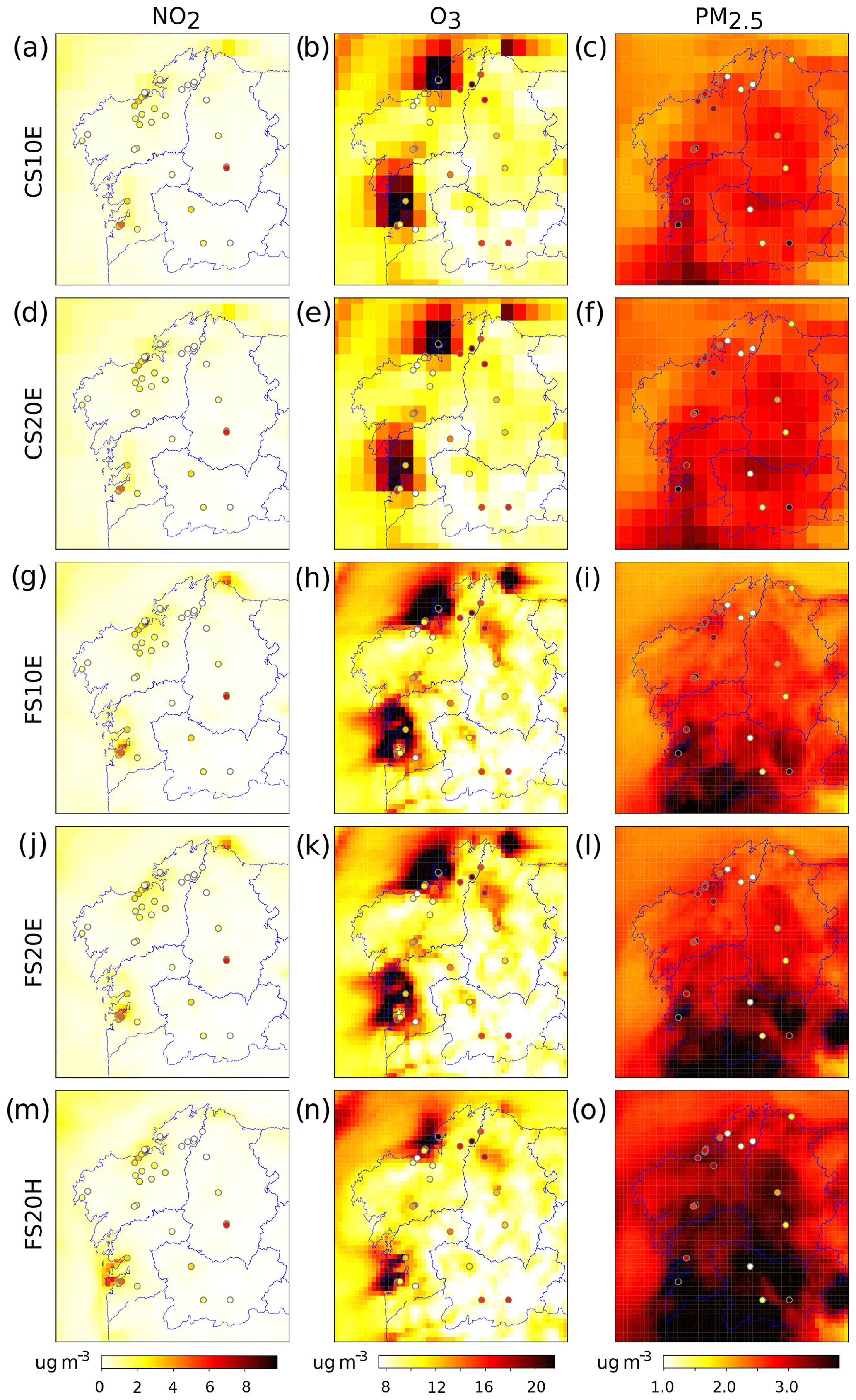
Figure 7 Observed (dots) vs. modeled (underlying pattern) temporal standard deviation values for the daily minimum concentrations of NO₂, O₃ and PM_2.5, as well as the five experiments marked with an asterisk in Table 3, all run with the SAPRC mechanism. The spatial verification results for each panel are provided in Table 4d.

Figure 7 and Table 4d show the respective verification results for the temporal standard deviation of the daily minimum concentrations. For NO₂ (Fig. 7, column 1), the model on average underestimates the temporal variability (SBIAS<0) and the associated spatial dispersion (SRATIO well below unity). With SR values ranging between 0.35 and 0.52 the model captures the spatial pattern of temporal variability to a certain degree. Results are insensitive to a vertical resolution increase (compare Fig. 7a with d and g with j) but systematically improve if the horizontal resolution is augmented (compare a with g and d with j). The temporal variability of the O₃ minima (Fig. 7, column 2) is on average well reproduced by the model (SBIAS≈0). However, the associated spatial pattern is missed (SR≈0) and the dispersion overestimated (SRATIO>1). Neither a horizontal nor a vertical resolution increase noticeably improves these results. The temporal variability of the PM_2.5 minima (Fig. 7, column 3) is also well reproduced on average and some skill is obtained for the respective spatial distribution. As for the NO₂ minima, the degree of spatial dispersion is also underestimated for the PM_2.5 minima (SRATIO<1) and can be improved by a horizontal resolution increase (compare panels c with i and f with l). Results for FS20H closely agree with those for FS20E, except for generally lower O₃ and higher PM_2.5 concentrations (compare the last two rows in Fig. 7).

3.2.2 Full temporal verification

Figure 8 shows the full temporal verification results for the daily minimum NO₂ and O₃ concentrations. For a correct interpretation of the results, it is important here to note that the observed minimum concentrations in our study region are generally low and that average differences of only a few micrograms per cubic meter (µg m⁻³) can translate into large percentage bias values.

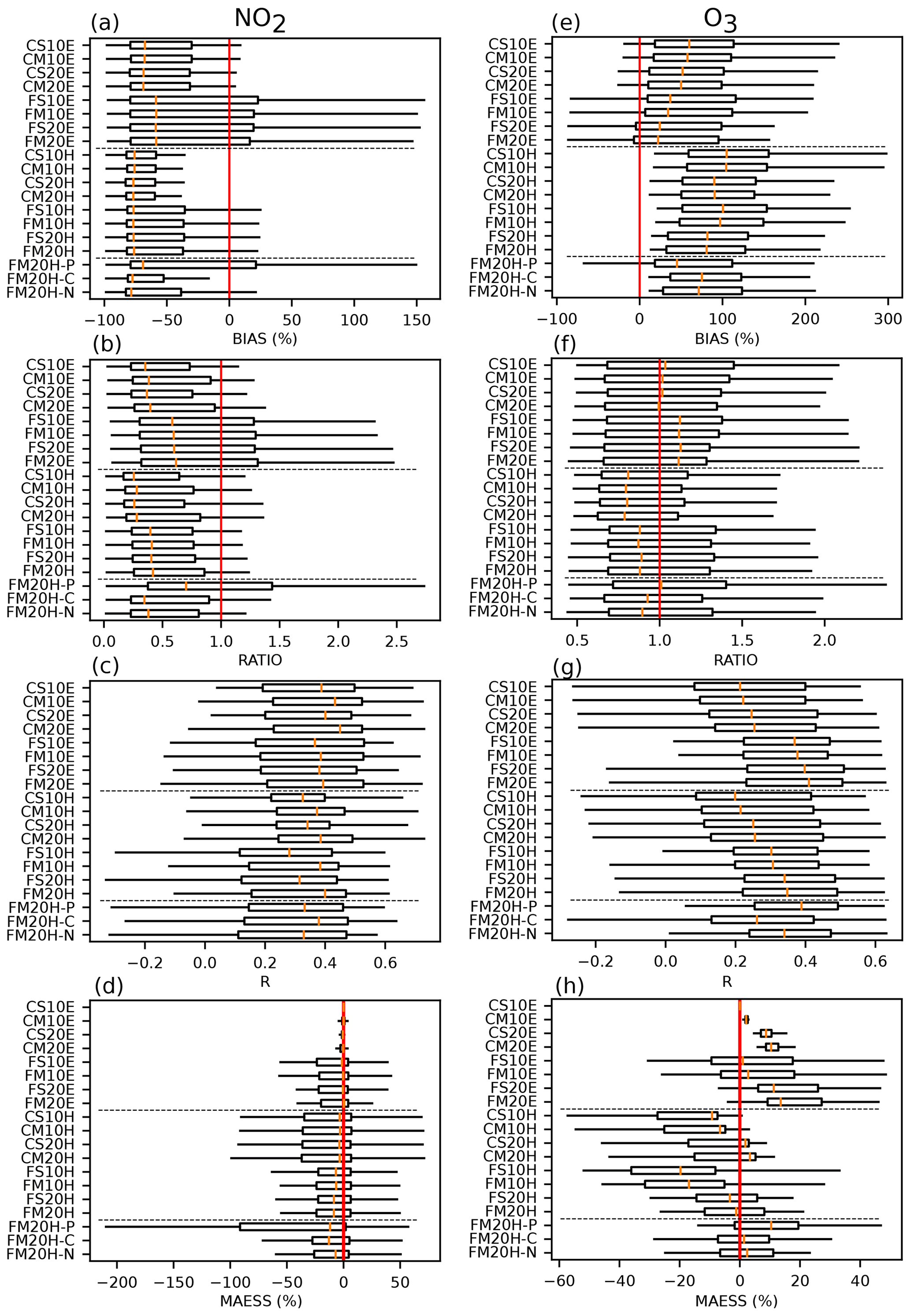
Figure 8 Temporal verification results for daily near-surface minimum NO₂ (a–d) and O₃ (e–h). (a, e) Percentage bias (BIAS), (b, f) Pearson correlation coefficient (R), (c, g) ratio of standard deviation (RATIO), (d, h) mean absolute error skill score (MAESS) with reference to the base experiment CS10E. Box plots are calculated upon the pointwise verification results at all available stations. Experiments are explained and grouped as in Table 3.

As can be seen from Fig. 8a and b, the temporal mean and standard deviation of the daily minimum NO₂ concentrations are considerably underestimated at nearly all stations in any of the applied experiments. The spatial median values for BIAS and RATIO can be improved with a horizontal resolution increase and either emission configuration 1 (FS10E, FM10E, FS20E and FM20E) or configuration 2 plus population downscaling (FM20H-P), implying that this kind of downscaling is key at this point. However, improvements in the spatial median can only be achieved at the expense of a large increase in the spatial spread of the results, which is in line with the findings obtained for the NO₂ maxima (see Sect. 3.1.2). For the correlation coefficient (Fig. 8c), emission configuration 1 performs better than configuration 2, full Melchior better than SAPRC and the coarse horizontal mesh better than the fine one. In comparison, an increase in vertical resolution from 10 to 20 layers is less efficient in improving the correlation. Coarse-resolution meteorological input data and missing biogenic emissions both slightly worsen the model performance for all applied verification measures (compare FM20H-C and FM20H-N with FM20H in panels a, c, e and g). When considering the MAESS (Fig. 8d), the spatial median performance for the base experiment (CS10E) cannot be improved by any of the applied alternative experiments, and the aforementioned growth in the results' spatial dispersion due to population downscaling can be clearly seen for FM20H-P.

Similar to the respective results for the maximum concentrations, daily minimum O₃ concentrations are also on average overestimated by the model (Fig. 8e), and the results for all verification measures can be improved by applying the full Melchior mechanism and 20 vertical layers (Fig. 8e to h). Contrary to the maxima, the spatial median performance for the O₃ minima can generally be further improved by applying a fine horizontal mesh, in which case the unwanted increase in spatial spread is less pronounced than for the maxima. The overall performance in terms of MAESS (Fig. 8h) is very satisfactory for the coarse-horizontal-resolution experiments run with 20 vertical layers (see CS20E and CM20E), which is in line with the results for the maxima. However, due to the aforementioned relatively weak increase in the spatial spread of the results, the use of a fine mesh is more tentative for the O₃ minima than for the maxima, particularly if emission configuration 1 is applied (compare CS20E, CM20E with FS20E and FM20E in Figs. 8h and 4h). Coarse-resolution meteorological input data and missing biogenic emissions both have negligible effects on the results. Population downscaling, however, leads to a systematic improvement (compare FM20H-C, FM20H-N and FM20H-P with FM20H in Fig. 8h).

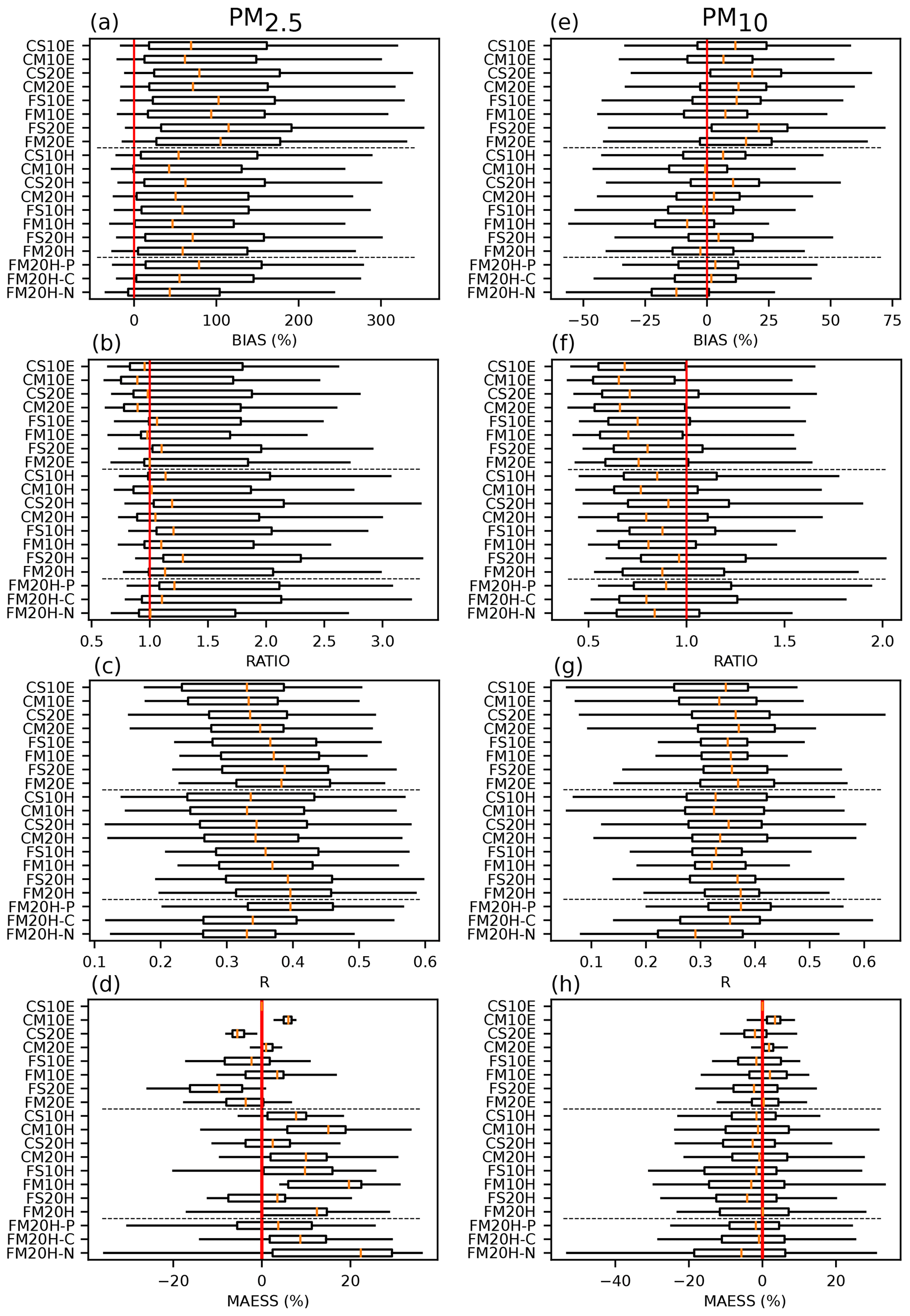
Figure 9 Temporal verification results for daily near-surface minimum PM_2.5 (a–d) and PM₁₀ (e–h). Row 1: percentage bias (BIAS), row 2: Pearson correlation coefficient (R), row 3: ratio of standard deviation (RATIO), row 4: mean absolute error skill score (MAESS) with reference to the base experiment CS10E. Box plots are calculated upon the pointwise verification results at all available stations. Experiments are explained and grouped as in Table 3.

The full temporal verification results for the PM_2.5 and PM₁₀ minima are displayed in Fig. 9. The model systematically overestimates the temporal mean PM_2.5 concentrations and also tends to overestimate the temporal variability (Fig. 9a and b). Using 20 vertical layers instead of 10 enhances the correlation coefficient on the one hand but, on the other, generally increases the bias and shifts the standard deviation ratio to values larger than unity (except for moving from CS10E to CS20E; see Fig. 9a–c). A horizontal resolution increase has similar effects, which are, however, larger in magnitude. Switching from SAPRC to full Melchior improves the results for all measures and nearly all experiments, and the overall performance gains as measured by MAESS are largest for this kind of switch (see panels a to d). When spatial median values are considered, the MAESS values obtained with emission configuration 2 are systematically better than those obtained with configuration 1 (see Fig. 9d). However, the spatial spread in the MAESS is larger for configuration 2 than for configuration 1. In comparison with FM20H, overall performance deteriorates for the population downscaling experiment (see FM20H-P), even more so for the coarse meteorological input experiment (see FM20H-C). Missing biogenic emissions improve the MAESS on average but also increase the spatial spread (see FM20H-N). Notably, the performance increase in the CM10E experiment (with respect to the base experiment CS10E) is positive at every station, which is rarely the case in the present study. Hence, the coarse horizontal mesh is again a straightforward option that already yields optimal results with a simple 10-layer setup if the full Melchior mechanism is applied.

For the PM₁₀ minima, emission configuration 2 yields smaller bias values and more favorable standard deviation ratios than configuration 1 (Fig. 9e and f) but weaker correlation coefficients (panel g). Using full Melchior instead of SAPRC and 20 instead of 10 vertical layers reduces the bias for all experiments, with both factors being of roughly equal importance for this pollutant and temporal aggregation. Correlation coefficients are also improved, but only for the experiments run with emission configuration 1. If emission configuration 2 is used, SAPRC yields roughly the same correlation coefficients as full Melchior (Fig. 9g). The standard deviation ratios are systematically better for SAPRC than for full Melchior and for 20 instead of 10 layers if the fine horizontal mesh is chosen. Regarding MAESS (Fig. 9h), performance losses caused by population downscaling or coarse-resolution meteorological input are less pronounced for the coarse particles than for the fine ones (compare FM20H-P and FM20H-C with FM20H in Fig. 9d and h). As for the fine particles, the “no biogenic emissions” experiment is also plagued by an increased spatial variability in the MAESS and, unlike the results for the fine particles, suffers from a spatial average performance decrease if compared to its base experiment (compare boxes and median values for FM20H-N with FM20H in Fig. 9d and h). As expected, the modeled mean values are more realistic when biogenic emissions are taken into account (compare FM20H with FM20H-N in Fig. 9e). As for the fine particles, optimal results are obtained with the coarse horizontal mesh run with only 10 layers and the full Melchior mechanism (see CM10E in panel Fig. 9h). Although the being second choice for the fine particles, emission configuration 1 is the first choice for the coarse ones.

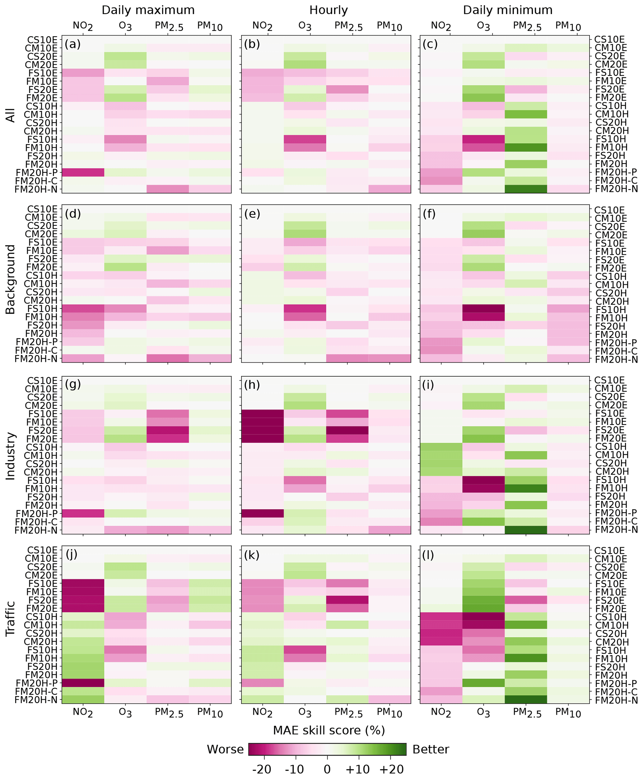
Figure 10 Spatial median mean absolute error skill score (MAESS) with respect to the base experiment CS10E for daily maximum, hourly or daily minimum concentrations (columns 1 to 3, respectively) at all available stations (row 1) or at background, industrial or traffic stations (rows 2 to 4, respectively).

3.3 Verification results per pollution source

Figure 10 shows the spatial median MAESS with reference to the base experiment CS10E for all locations (row 1) and separately for background, industry and traffic locations (rows 2 to 4). The first column refers to the results for daily maximum concentrations, the second to hourly concentrations and the third to daily minimum concentrations. Improvement over the base experiment is indicated by green and worsening by red shading.

As can bee seen from the predominantly red shading in the first two columns of Fig. 10, the base experiment CS10E already provides a good overall skill, which is difficult to exceed when considering daily maximum or hourly concentrations. Among all suggested model improvement factors, the use of 20 instead of 10 vertical layers yields the most balanced increases in spatial median performance irrespective of the applied chemical mechanism (see CS10E and CM20 in these columns). Switching from coarse to high horizontal resolution leads to large performance increases for particular pollutants and/or station types, but only at the expense of performance decreases for the remaining species and sites and thus to unbalanced results.

Irrespective of the applied emission configuration and number of vertical layers, the best results for the maximum and hourly NO₂ values are obtained with a coarse horizontal resolution, except at traffic stations where the fine horizontal mesh yields better results if, importantly, emission configuration 2 is used without population downscaling (compare FS10E, FM10E, FS20E and FM20E in Fig. 10j and k). At traffic and industry sites, the worst results for the NO₂ maxima and hourly data are obtained with the fine horizontal mesh and emission configuration 1 (relying on population and traffic downscaling) as well as with configuration 2 plus population downscaling (note the similarity between FS10E, FM10E, FS20E, FM20E and FM20H-P in Fig. 10a, b, g, h, j, k). Hence, this kind of downscaling is not advantageous in these cases.

For daily minimum NO₂, the coarse horizontal resolution is again the best choice, but only in combination with emission configuration 1 (see CS10E, CM10E, CS20E and CM20E in panels c, f, i and l). Using the coarse horizontal resolution with configuration 2 instead yields heterogeneous results; i.e., better results at industrial sites are contrasted by worse results at traffic sites (compare CS10H, CM10H, CS20H and CM20H in panel i with panel l).

For O₃, emission configuration 1 performs systematically better than configuration 2. Among the emission configuration 2 experiments, it is again the population downscaling experiment that most closely resembles the results from the configuration 1 experiments (compare experiments ending in E with FM20H-P). Importantly, using 20 instead of 10 vertical layers yields performance gains in virtually any case, i.e., irrespective of the applied emission configuration, horizontal mesh, chemical mechanism, temporal aggregation and pollution source type, and is consequently the most robust model improvement factor for surface O₃ concentrations assessed here. Second best in this context is the use of the full Melchior mechanism instead of SAPRC. Note also that the results for the maxima and hourly data are less similar to each other than for the remaining pollutants.

As opposed to the findings for O₃, emission configuration 2 is the better choice for PM_2.5, particularly considering daily minimum concentrations at all kind of sites, as well as maximum and hourly concentrations at industrial and traffic sites. The effects of a vertical resolution increase are heterogeneous. At background sites (see second row in Fig. 10 and also Supplement Fig. S2), results are improved for the daily maxima but deteriorate for the minima, with very few effects on the hourly concentrations. At industrial and traffic sites, however, results generally worsen for this factor. At background sites, SAPRC is generally superior to full Melchior, whereas the opposite is found at industrial and traffic sites. As for O₃, a horizontal resolution increase is not advantageous for PM_2.5 either, except for the daily minimum concentrations at industrial and traffic sites when using emission configuration 1.

Model sensitivity is generally lower for PM₁₀ than for the other three pollutants. The largest performance gains are obtained for daily maximum concentrations, particularly at traffic sites, if the fine horizontal mesh is used in combination with 20 vertical layers and emission configuration 1 (see experiments FS20E and FM20E in panels a, d, g, and j). The same mesh, however, yields the largest performance losses for minimum concentrations at background sites if emission configuration 2 is applied (see panel f). Although the differences are generally weak, the SAPRC mechanism is preferable for maximum and hourly concentrations, whereas full Melchior is preferable for the minima.

Among the three specific sensitivity experiments, the population downscaling (FM20H-P) experiment exhibits the largest performance deviations from the common base experiment (FM20H), followed by the “no biogenic emissions” (FM20H-N) and coarse meteorology (FM20H-C) experiments. FM20H-P performs particularly bad for maximum and hourly NO₂ concentrations at industry and traffic sites (see panels g, h, j and k) and particularly well for minimum O₃ concentrations at traffic sites (see panel l). Curiously, among all considered experiments, FM20H-N yields the best results for minimum PM_2.5 concentrations at industry and traffic sites (see panels i and l) and for maximum NO₂ concentrations at traffic sites (see panel j). The good skill scores at these station types arise from error compensation effects. Namely, the positive bias is for minimum PM_2.5, which is smaller at traffic and industry sites than at background sites because the observed concentrations are higher there, and is improved when biogenic emissions are turned off, which translates into better MAESS values. For maximum NO₂, removing this kind of emission enhances the temporal correlation, brings the standard deviation closer to unity and finally also improves the MAESS. This, in turn, means that the inclusion of biogenic emissions in the remaining experiments deteriorates the temporal variability and day-to-day sequence of the modeled minimum NO₂ time series if compared with observations. At background sites, however, the NO₂ and PM_2.5 maxima are generally underestimated by the model, and the exclusion of biogenic emissions further increases this negative bias (see Fig. 10d and Fig. S2). The pronounced reduction of the O₃ maxima at background sites in the FM20H-N experiment, compared with FM20H, points to an active role of biogenic VOCs in this case (see Fig. S2e). For FM20H-C, deviations from the base experiment are largest for the minima at industry sites and are otherwise generally weak (see Fig. 10i).

4 Discussion and conclusions

In this study, a series of 19 sensitivity experiments was carried out with the chemical weather forecasting model CHIMERE over the northwestern Iberian Peninsula for the 2018 summer season in order to assess the model's capability to reproduce in situ NO₂, O₃, PM₁₀ and PM_2.5 surface concentrations on a daily to hourly timescale. The range of applied model experiments covers the effects of distinct emission configurations, horizontal and vertical resolution setups, and model chemistries. With the help of three secondary experiments, the impact of population downscaling, coarse-resolution meteorological input data and missing biogenic emissions is discussed in addition. All these experiments were driven by meteorological data from WRF and chemical boundary data from ECMWF's C-IFS.

The obtained results are very heterogeneous, and the applied model improvement efforts, often associated with considerable computational costs, generally do not lead to an unrestricted model improvement. For most efforts, verification results improve for some aspects but worsen for others. Nonetheless, one single factor has been identified that improves the model in a systematic way, returning better results for virtually all aspects of the verification.

The first take-home message is that the use of an up-to-date and sophistically downscaled anthropogenic emission inventory (configuration 1: EMEP for the year 2017 downscaled with land use, population and traffic proxies as well as large point sources), if compared to an older inventory downscaled with basic options (configuration 2: HTAP v2.2 for the year 2010 downscaled with land use only), improves the modeled O₃ and PM₁₀ concentrations but deteriorates the results for NO₂ and PM₁₀. This is in line with Russo et al. (2019) in the sense that an upgraded emission inventory does not necessarily improve the modeled pollutant concentrations with respect to observations in all aspects.

Second, heterogeneous results are obtained for the performance changes associated with the chemical mechanism. While the performance for NO₂ is practically unrelated to the chosen mechanism, the full Melchior mechanism is preferable to SAPRC if O₃ concentrations – at any temporal scale – are considered. For particulate matter, SAPRC is preferable for the daily maxima and hourly concentrations and full Melchior for the daily minima.

Third, an increase in the horizontal resolution of the CHIMERE domain and associated emissions from $\mathrm{0.15}{}^{\circ }\times \mathrm{0.15}{}^{\circ }$ to $\mathrm{0.05}{}^{\circ }\times \mathrm{0.04}{}^{\circ }$ does not lead to a systematic model improvement but rather to a large increase in the spatial variability of the results. In line with Valari and Menut (2008), we have indications that this is caused by the noise increase in high-resolution meteorological input data and, to an even larger degree, by the population downscaling procedure used to reallocate the raw data from the applied anthropogenic emission inventories on the subgrid scale. If this kind of downscaling is used, the model overestimates the temporal mean value of the daily maximum and hourly concentrations at traffic and industry sites. The same applies to the temporal standard deviation, i.e., to the model's capability to simulate the degree of temporal variability from one day to another.

Contrary to the effects obtained with an increased horizontal resolution, the use of 20 instead of 10 vertical layers within the lower to middle troposphere (999 to 500 hPa) systematically improves the model results for nearly all aspects of the verification.

All together, and as long as top-down emission inventories at a relatively coarse spatial and temporal resolution are applied, we recommend the use of 20 model layers together with a horizontal resolution not much finer than the native resolution of the inventory. In this context, the resolution of the coarse domain applied here ($\mathrm{0.15}{}^{\circ }\times \mathrm{0.15}{}^{\circ }$) may not be optimal and in future studies should be approximated to the native grid of the emission inventory (i.e., $\mathrm{0.1}{}^{\circ }\times \mathrm{0.1}{}^{\circ }$ for both HTAP and EMEP) in order to see whether the results can be further improved. Likewise, a region-specific optimization of the downscaling procedures used to reallocate raw emissions on the subgrid scale according to proxy data for population and traffic density would likely yield better results for the northwestern Iberian Peninsula, particularly concerning the NO₂ and PM_2.5 concentrations.

As a final remark, the present study has explored a broad range of model performance factors with empirical methods, mainly to provide practical recommendations for the numerical modeling community. In the future, our results should be complemented by analytic in-depth studies focusing on single factors.