The shared socio-economic pathway (SSP) greenhouse gas concentrations and their extensions to 2500

Anthropogenic increases in atmospheric greenhouse gas concentrations are the main driver of current and future climate change. The integrated assessment community has quantified anthropogenic emissions for the shared socio-economic pathway (SSP) scenarios, each of which represents a different future socio-economic projection and political environment. Here, we provide the greenhouse gas concentrations for these SSP scenarios – using the reduced-complexity climate–carbon-cycle model MAGICC7.0. We extend historical, observationally based concentration data with SSP concentration projections from 2015 to 2500 for 43 greenhouse gases with monthly and latitudinal resolution. CO₂ concentrations by 2100 range from 393 to 1135 ppm for the lowest (SSP1-1.9) and highest (SSP5-8.5) emission scenarios, respectively. We also provide the concentration extensions beyond 2100 based on assumptions regarding the trajectories of fossil fuels and land use change emissions, net negative emissions, and the fraction of non-CO₂ emissions. By 2150, CO₂ concentrations in the lowest emission scenario are approximately 350 ppm and approximately plateau at that level until 2500, whereas the highest fossil-fuel-driven scenario projects CO₂ concentrations of 1737 ppm and reaches concentrations beyond 2000 ppm by 2250. We estimate that the share of CO₂ in the total radiative forcing contribution of all considered 43 long-lived greenhouse gases increases from 66 % for the present day to roughly 68 % to 85 % by the time of maximum forcing in the 21st century. For this estimation, we updated simple radiative forcing parameterizations that reflect the Oslo Line-By-Line model results. In comparison to the representative concentration pathways (RCPs), the five main SSPs (SSP1-1.9, SSP1-2.6, SSP2-4.5, SSP3-7.0, and SSP5-8.5) are more evenly spaced and extend to lower 2100 radiative forcing and temperatures. Performing two pairs of six-member historical ensembles with CESM1.2.2, we estimate the effect on surface air temperatures of applying latitudinally and seasonally resolved GHG concentrations. We find that the ensemble differences in the March–April–May (MAM) season provide a regional warming in higher northern latitudes of up to 0.4 K over the historical period, latitudinally averaged of about 0.1 K, which we estimate to be comparable to the upper bound (∼5 % level) of natural variability. In comparison to the comparatively straight line of the last 2000 years, the greenhouse gas concentrations since the onset of the industrial period and this studies' projections over the next 100 to 500 years unequivocally depict a “hockey-stick” upwards shape. The SSP concentration time series derived in this study provide a harmonized set of input assumptions for long-term climate science analysis; they also provide an indication of the wide set of futures that societal developments and policy implementations can lead to – ranging from multiple degrees of future warming on the one side to approximately 1.5 ^∘C warming on the other.

1 Introduction

The climate modelling community periodically undertakes large model intercomparison exercises with the latest and most sophisticated set of climate models, to gain a better understanding of the response of the climate system to a range of potential emission or concentration scenarios (Taylor et al., 2012; Meehl et al., 2007). The atmosphere–ocean general circulation models (AOGCMs) are physical climate models that may include biogeochemical model components, such as vegetation or some atmospheric chemistry, but they are not able to project CO₂ concentrations from emissions due to an incomplete, imbalanced, or non-existent carbon cycle. The climate models that have this ability to project CO₂ concentrations from emissions are often referred to as Earth system models (ESMs) (Lawrence et al., 2016; Jones et al., 2016). These ESMs are also often run in “CO₂-concentration-driven mode” for computational ease and to allow for an easier separation between carbon cycle feedbacks and climate responses. As of today in phase 6 of the Coupled Model Intercomparison Project (CMIP6) (Eyring et al., 2016), both AOGCMs and ESMs use concentrations from all non-CO₂ greenhouse gases to perform multi-gas experiments (such as the future scenario projections) due to either missing non-CO₂ gas cycles or a prohibitive computational burden.

This study provides and describes the standardized set of greenhouse gas (GHG) concentration futures for CO₂, CH₄, N₂O, and 40 other minor greenhouse gases. For the historical period, this GHG concentration data for CMIP6 were provided by the companion paper Meinshausen et al. (2017). This study provides the GHG concentration data until 2100 on the basis of the emission scenarios derived from socio-economically explicit integrated assessment models (IAMs) under the shared socio-economic pathway (SSP) framework (Gidden et al., 2019). We also provide an extension of the concentration data until 2500 on the basis of simplified assumptions.

These concentrations datasets are part of the protocols for several CMIP6 experiments, most notably ScenarioMIP (O'Neill et al., 2016) and AerChemMIP (Collins et al., 2017), that require concentration-driven runs (see search.es-doc.org for a full description). While greenhouse gases are arguably the most important influence of humankind on future climate in terms of radiative forcing, there is a wide range of other forcers, including anthropogenic aerosols (Hoesly et al., 2018), land use patterns, aerosol optical properties (Stevens et al., 2017), and natural forcers like solar (Matthes et al., 2017) and volcanic effects (Toohey et al., 2016). These forcers are described in the companion papers and compiled in the input4mip interface to be used for the historical and future ESM experiments (Durack and Taylor, 2019), available on https://esgf-node.llnl.gov/projects/input4mips/ (last access: 20 June 2020).

Our future greenhouse gas concentration datasets from 2015 onwards are provided for a total of nine SSP scenarios. These nine scenarios comprise five high-priority scenarios for the Sixth Assessment report by the IPCC report, which is the group of four “Tier 1” scenarios highlighted in ScenarioMIP (O'Neill et al., 2016) in addition to the SSP1-1.9 scenario that reflects most closely a 1.5 ^∘C target under the Paris Agreement. Specifically, these “high-priority” scenarios for IPCC AR6 are, firstly, the SSP1-2.6 “2 ^∘C scenario” of the “sustainability” SSP1 socio-economic family, whose nameplate 2100 radiative forcing level is 2.6 W m⁻². This SSP1-2.6 scenario approximately corresponds to the previous scenario generation Representative Concentration Pathway (RCP) 2.6. Secondly, the  SSP2-4.5 of the “middle of the road” socio-economic family SSP2 with a nominal 4.5 W m⁻² radiative forcing level by 2100 – approximately corresponding to the RCP-4.5 scenario. Thirdly, the SSP3-7.0 scenario is a medium-high reference scenario within the “regional rivalry” socio-economic family, while the final Tier 1 scenario, SSP5-8.5, marks the upper edge of the SSP scenario spectrum with a high reference scenario in a high fossil-fuel development world throughout the 21st century. The additional high-priority scenario that IPCC AR6 considers is SSP1-1.9 to better reflect the research regarding the Paris Agreement's 1.5 ^∘C target. It should be noted that the radiative forcing labels, such as “2.6” in the SSP1-2.6 scenario, are indicative “nameplates” only, approximating total radiative forcing levels by the end of the 21st century. Those labels are merely indicative, given that actual radiative forcing uncertainties (and differences across ESMs that implement the same concentrations, aerosol abundances, ozone fields, and land use patterns) are substantial.

In addition to these five high-priority scenarios, we provide concentrations for four additional SSP scenarios, namely the three remaining “Tier 2” ScenarioMIP experiments, featuring a low reference scenario SSP4-6.0 within the socio-economic context of an “inequality”-dominated world, as well as its moderate mitigation scenario SSP4-3.4. Similarly, there is the geophysically interesting emission “overshoot” scenario, SSP5-3.4-OS, as it initially follows the high-emission SSP5-8.5 scenario until 2030 before exhibiting the steepest annual reduction rates of all SSP scenarios and the most net negative emissions by 2100. Lastly, we also consider the SSP3-7.0-LowNTCF variant of the SSP3-7.0 scenario with reduced near-term climate forcer (NTCF) emissions. Given that the SSP3-7.0 scenario is the one with the highest methane and air pollution precursor emissions, the SSP3-7.0-LowNTCF variant investigates an alternative pathway for the AerChemMIP intercomparison project (Collins et al., 2017) that exhibits very low methane, aerosol, and tropospheric-ozone precursor emissions – approximately in line with the lowest other SSP scenarios for those species like SSP1-1.9 and SSP1-2.6. Note that the NTCF nomenclature is equivalent to the term short-lived climate forcer, SLCF, which is now more commonly used by the research community and IPCC context.

The presented historical global-mean and hemispheric-mean surface mole fractions in this study transition smoothly from the end of the historical dataset (Meinshausen et al., 2017), 2014, into the start of the projections, 2015. Also, the latitudinal gradient and seasonality, and their temporal evolution, are consistent with the historical dataset – which in all cases is tied directly to past measurements. We used a reduced-complexity carbon cycle model, MAGICC (Meinshausen et al., 2011c, a), to produce global-mean future greenhouse gas concentration time series for each of the considered SSPs. The same model, albeit an earlier version, was also previously used to provide the RCP greenhouse gas concentrations projections (Meinshausen et al., 2011b). The MAGICC version used for this study (version 7.0) is calibrated to closely represent C4MIP carbon cycle responses and includes a permafrost module (Schneider von Deimling et al., 2012) and updated radiative forcing and non-CO₂ gas cycle parameterizations (in particular for CH₄ and N₂O) that represent recent literature findings (Prather et al., 2012; Holmes et al., 2013). The calibrated carbon cycle of MAGICC has previously been shown to reflect the CMIP5 ESM response range well (Friedlingstein et al., 2014). Given the nearly 2-year time difference between the completion of historical and future greenhouse gas concentrations, we also updated the historical observational datasets to reflect observations until early 2018 for CO₂, CH₄, and N₂O, as well as most other gases considered here.

This study first describes the methods with separate parts for the updated observational data until 2018 (Sect. 2.1), the emission input data from the IAM scenarios and the input preparation steps undertaken (Sect. 2.2), the extensions of the emissions and concentrations beyond 2100 (Sect. 2.3), the MAGICC model setup (Sect. 2.4), and the projections of latitudinal gradients (Sect. 2.5) and seasonality (Sect. 2.6). We also provide a new simplified formula to reflect the Oslo Line-By-Line model (OLBL) radiative forcing results (Etminan et al., 2016) in order to provide the radiative forcing aggregation of the output (Sect. 2.7) and discuss additional methodological steps (Sect. 2.8). We then show the results and compare these to other recent observational datasets (Sect. 3 “Results”). A discussion section follows (Sect. 4 “Discussion”), which includes a closer look at the two most dominant GHG forcers, CO₂ and CH₄, and their correlation (Sect. 4.1), a discussion on the most recent GHG concentration developments (Sect. 4.2), and the comparison with RCP concentrations (Sect. 4.4). We describe the limitations of the dataset (Sect. 5), which includes issues like the integration of observational and modelled future data, missing uncertainty estimates, potential biases in future seasonality and latitudinal gradients, and a lack of reference scenarios for Montreal-controlled substances. Section 6 concludes the paper.

2 Methods

As for the historical concentrations, we provide 43 greenhouse gas future concentration projections, namely CO₂, CH₄, N₂O, 17 ozone-depleting substances (namely CFC-11, CFC-12, CFC-113, CFC-114, CFC-115, HCFC-22, HCFC-141b, HCFC-142b, CH₃CCl₃, CCl₄, CH₃Cl, CH₂Cl₂, CHCl₃, CH₃Br, Halon-1211, Halon-1301, and Halon-2402) and 23 other fluorinated compounds (namely 11 hydrofluorocarbons (HFCs) – HFC-134a, HFC-23, HFC-32, HFC-125, HFC-143a, HFC-152a, HFC-227ea, HFC-236fa, HFC-245fa, HFC-365mfc, HFC-43-10mee; NF₃, SF₆, and SO₂F₂; and nine perfluorocarbons (PFCs) – CF₄, C₂F₆, C₃F₈, C₄F₁₀, C₅F₁₂, C₆F₁₄, C₇F₁₆, C₈F₁₈, and c-C₄F₈). Our projections refer to atmospheric dry-air mole fractions as do the historical data presented in Meinshausen et al. (2017), even though the projections are sometimes loosely referred to as “concentrations”. For CO₂, the usual unit is parts per million (ppm), for CH₄ and N₂O, the usual unit is parts per billion (ppb), and other gases are usually denoted in parts per trillion (ppt).

2.1 Updated observational data

The historical concentrations (until the end of 2014) were derived from various observational datasets of greenhouse gas concentrations or literature studies in the case of some of greenhouse gases with lower concentrations. The observational data were binned by latitudinal and longitudinal boxes, averaged for monthly values, and complemented by interpolations. The historical time series for every greenhouse gas were separated into three elements as part of the spatio-temporal binning: (i) latitudinal gradient, (ii) seasonality pattern, and (iii) global mean. This separation then permitted the use of longer observational time series, such as the high-latitudinal CH₄ firn data – implicitly correcting for the high-latitude differences to the global mean that one would expect. Interpolations, regressed latitudinal gradients, and seasonality patterns were employed to derive the historical dataset, but no gas cycle models.

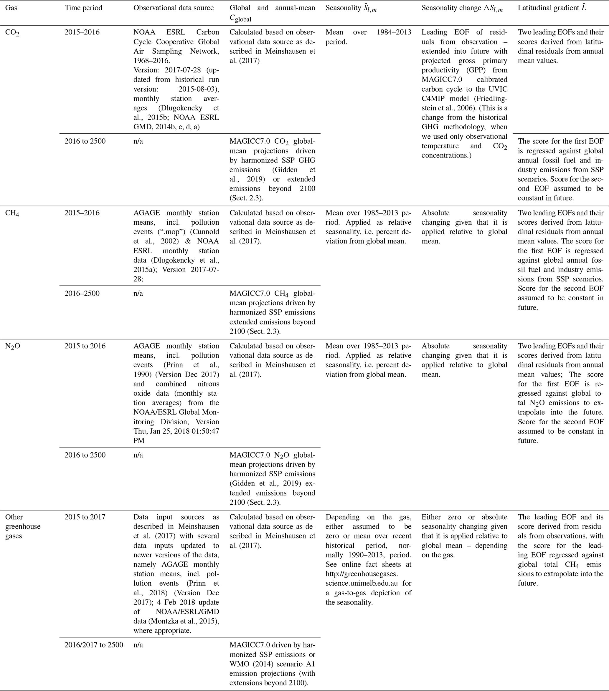
With additional observational data being available for 2015, 2016, and 2017, the previously used observational data sources from the AGAGE and NOAA networks (Dlugokencky, 2015a, b; Prinn et al., 2018), including multiple NOAA ESRL Global Monitoring Laboratory (https://www.esrl.noaa.gov/gmd/, last access: 14 July 2020) flask measurements, were updated and used to determine the initial years of the future concentration time series. The result of this is that – depending on the gases – the same concentrations are used across all nine SSPs in the initial years (Table 1). As outlined below, we employed MAGICC7.0 and its calibrated gas cycles to produce concentration time series from SSP emissions beyond the observationally based period.

Table 1 Derivation and construction of future CMIP6 mixing ratio fields for the greenhouse gas concentration series from 2015 onwards. Note that in addition to the steps shown below, a post-processing step was implemented to scale any differences in the December 2014 values between the raw future data and the previously submitted historical greenhouse gas concentration data. Those data differences in monthly latitudinal values for December 2014 were linearly scaled to zero until December 2015 in order to provide for a smooth transition between historical and future datasets (Sect. 2.8). See Sect. 2.1 for a description of how the observational data were updated. n/a – not applicable

2.2 Emission data and their harmonization

For the emission-driven MAGICC7 runs that produce the future global-mean greenhouse gas time series, we use the SSP emission data for CO₂, CH₄ and N₂O, HFCs, PFCs, and SF₆ which are available from the SSP database at IIASA (https://tntcat.iiasa.ac.at/SspDb, last access: 20 June 2020). This emission data have already been subject to several categorization and harmonization steps to obtain regionally consistent (in the case of CO₂ and CH₄) and sectorally resolved data (for more details, see Gidden et al., 2019). We complemented those harmonization steps to consider the following species in the five RCP regions (OECD90, REF (economies in transition), LAM (Latin America), MAF (Middle East and northern Africa) and ASIA): CO₂, CH₄, and N₂O in addition to black carbon (BC), carbon monoxide (CO), ammonium (NH₃), non-CH₄ volatile organic compounds (NMVOCs), nitrates (NO_x), organic carbon (OC), and sulfate aerosol (SO_x). For those 10 species, we also distinguished between fossil and industrial sources and land-use-related sources.

Regional land use CO₂ emissions are not provided in the SSP database (Gidden et al., 2019), so we downscaled to the RCP regions based on historical regional emission shares in the year 2015. Given land use CO₂ emissions can be negative in some SSP scenarios, a simple scaling approach in the regional harmonization would yield unrealistic results (i.e. regions with low or negative current net land use emissions, like the OECD, would end up with positive emissions and the other world regions would be strongly negative in the future). Instead, we applied a normalization that assumes a negative 1.5 GtC base level against which historical regional emission shares are continued into the future, scaled with global emissions.

Mathematically, the constant regional scaling factor is hence applied to the offset emission level, so that the future regional emissions E_r(y) in year y are as follows:

$$\begin{array}{l}{E}_{\mathrm{r}}\left(y\right)=E_{\mathrm{g}}\left(\mathrm{2015}\right)\times s_{\mathrm{2015}}+\left(E_{\mathrm{g}}\left(y\right)-E_{\mathrm{g}}\left(\mathrm{2015}\right)\right)\times r,\\ \text{where}\\ r=\frac{E_{\mathrm{r}}\left(\mathrm{2015}\right)+\mathrm{1.5}}{{\sum }_{r=\mathrm{1}}^n(E_{\mathrm{r}}\left(\mathrm{2015}\right)+\mathrm{1.5})},\end{array}$$

with r being the regional share of emissions relative to that 1.5 GtC offset level, s being the regional share of emissions in 2015 relative to zero, i.e. $s_{\mathrm{2015}}=E_{\mathrm{r}}\left(\mathrm{2015}\right)/E_{\mathrm{g}}\left(\mathrm{2015}\right)$, E_r(y) being the regional emissions in year y, and E_g(y) being the global emissions, i.e. the sum of the n regional emissions. Specifically, the factors s₂₀₁₅ and r for were the following for the regions Asia, Latin America, the Middle East and Africa, OECD-90, and economies in transition: 0.483, 0.282, 0.189, 0.043, and 0.003 for s₂₀₁₅ and 0.232 0.209, 0.199, 0.182, and 0.178 for r, respectively. This choice has little effect because the regional split up of CO₂ emissions only marginally and indirectly affects the latitudinal concentrations in our chosen method. A very small difference arises for different regional land use CO₂ emission assumptions because MAGICC7 scales albedo effects with land use CO₂ emissions and these albedo effects impact temperatures and in turn the carbon cycle again.

Land-use-related CH₄ and fossil and industrial CO₂ and CH₄ emissions were already harmonized with historical emissions and also regionally available (Gidden et al., 2019, 2018). N₂O emissions were only available as a global total from the SSP database based on PRIMAP (Gütschow et al., 2016), which is why we assume to be constant regional and sectoral emission shares. This assumption does not have a bearing on final global concentrations.

For the emissions of fluorinated gases that are listed in the Kyoto Protocol and considered here (PFCs, HFCs, and SF₆), namely C₂F₆, CF₄, HFC-125, HFC-134a, HFC-143a, HFC-227ea, HFC-23, HFC-245fa, HFC-43-10mee, and SF₆, MAGICC7 takes the global and aggregated SSP emissions of the gas baskets as inputs, as provided by the IAM modellers using constant emission shares based on a future gas-specific scenario by Guus Velders (Velders et al., 2015) and described in Gidden et al. (2019). The basket of PFCs, HFCs, and SF₆ is reported in the SSP database at IIASA (https://tntcat.iiasa.ac.at/SspDb/, last access: 20 June 2020). Some few data points were corrected in consultation with the respective IAM modelling teams, namely the SSP1-1.9 emission level in 2100 for CF₄ and C₂F₆, for which we assumed the rate of decline prolonged from the 2080 to 2090 to the 2090 to 2100 period. HFC-32 emissions were complemented from a Kigali Agreement-consistent scenario, which has also been derived from the scenarios by Velders et al. (2015). Those scenarios were published until 2050 and we use in addition an extension up to 2100 by proportional downscaling of the global warming potential (GWP)-weighted HFC basket – using SSP GDP and population data with an assumption of constant GDP and population after 2100.

The ozone-depleting substances controlled under the Montreal Protocol, namely CFC-11, CFC-12, CFC-113, CFC-114, CFC-115, HCFC-22, HCFC-141b, HCFC-142b, CH₃Br, CH₃Cl, CH₃CCl₃, CCl₄, Halon-1202, Halon-1211, Halon-1301, and Halon-2402, are here assumed to follow the WMO 2014 scenario (WMO, 2014) from 1951 to 2099, as presented in detail in Velders and Daniel (2014). For times before 1951 and after 2099, the previous WMO A1 Baseline emission scenario from the year 2006 (WMO, 2006) is assumed, which is near-zero and close to the respective WMO 2014 values in 1951 and 2099.

Harmonized emissions of aerosol and ozone precursor species are also available for the SSP scenarios (Hoesly et al., 2018) but not discussed in this paper. These non-GHG emissions are used here as part of the complete scenario specification needed to produce future temperature and GHG concentration pathways.

2.3 Extension of emissions and concentrations beyond 2100

In 2011, the RCPs were extended beyond 2100 to provide the basis for longer-term scenario studies (Meinshausen et al., 2011b), then called “extended concentration pathways” (ECPs). Studying this longer-term behaviour of the climate system is of interest for quantities that exhibit a strong long-term commitment or non-linear behaviour (e.g. sea level rise, ice sheet dynamics). The RCP concentration extensions were – for some gases and scenarios – based on pragmatic extensions of emissions, like an RCP8.5 CO₂ emission stabilization from 2100 to 2150 with a subsequent ramp-down until 2250. For other RCPs, concentrations were held constant and the inverse CO₂ emissions exhibited a near-exponential decline.

Here, we present the extensions beyond 2100 of the ScenarioMIP and AerChemMIP SSPs (although we do not use a new acronym like ECPs at the time of the RCPs). The final choices differ, in some respects, from the initial sketch of these extensions that was offered in the ScenarioMIP overview paper (O'Neill et al., 2016). As described below, the collaborative exercise by the IAM modellers and MAGICC team updated the original SSP extension design. In summary, the extension principles are as follows:

1. From 2100 onwards, net negative fossil CO₂ emissions are brought back to zero during the 22nd century, while positive fossil CO₂ emissions are ramped down to zero by 2250.

2. Land use CO₂ emissions are brought back to zero by 2150.

3. Non-CO₂ fossil greenhouse gas emissions are ramped down to zero by 2250.

4. Land-use-related non-CO₂ emissions are held constant at 2100 levels.

In the initial ScenarioMIP design (O'Neill et al., 2016), fossil CO₂ emissions for SSP5-3.4-OS and SSP1-2.6 are negative at 2100 levels until 2140 and gradually increase to zero until 2190 and 2185, respectively (Fig. 2a). We did not assume permanent net-negative CO₂ emissions to maintain proximity to the original scenario design in the light of biophysical and economic limits of negative emissions, as well as potential side effects (Fuss et al., 2018; Smith et al., 2016). For all scenarios with net negative fossil fuel extensions, we implemented extensions assuming constant emissions until 2140 (as suggested) but reaching zero emissions in 2190. The only exception is the SSP5-3.4-OS scenario, which was ramped back to zero by a slightly earlier date (2170) so that fossil and land use emissions (in combination with MAGICC7.0's default setting – see Sect. 2.4) met the design criteria of an approximate merge with SSP1-2.6 concentrations in the longer-term, i.e. after 2150.

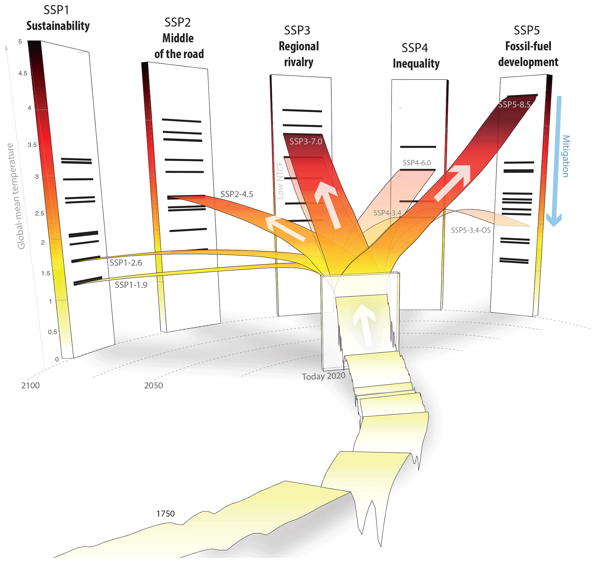
Figure 1 The SSP scenarios and their five socio-economic SSP families. Shown are illustrative temperature levels relative to pre-industrial levels with historical temperatures (front band), current (2020) temperatures (small block in middle), and the branching of the respective scenarios over the 21st century along the five different socio-economic families. The small black horizontal bars on the 2100 pillars for each SSP indicate illustrative temperature levels (obtained by the MAGICC7.0 default setting used to produce the GHG concentrations) for the range of SSP scenarios that were available from the IAM community at the time of creating the benchmark SSP scenarios. The more opaque bands over the 21st century indicate the five SSP scenarios SSP1-1.9, SSP1-2.6, SSP2-4.5, SSP3-7.0, and SSP5-8.5 that are used as priority scenarios in IPCC. The more transparent bands indicate the remaining “Tier 2” SSP scenarios, namely SSP3-7.0-LowNTCF (used in AerChemMIP), SSP4-3.4, SSP4-6.0, and SSP5-3.4-OS. Also shown is a blue indicative bar on the right side, indicating the effect of mitigation action, which reduces temperature levels in 2100 and throughout the 21st century – depending on the respective reference scenario and level of mitigation.

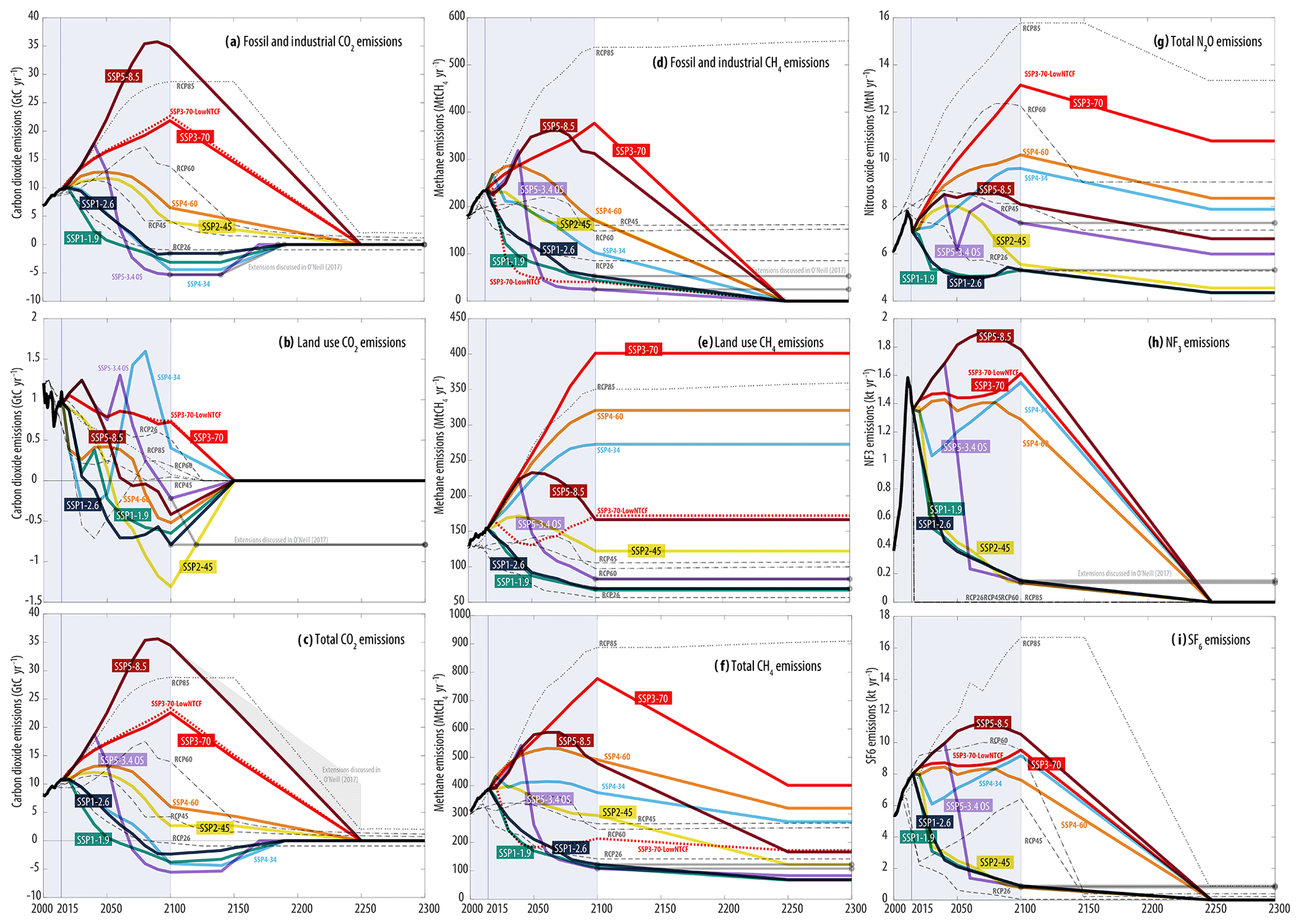
Figure 2 The anthropogenic emission scenarios to derive SSP concentration scenarios for CO₂ (a–c), CH₄ (d–e), nitrous oxide (f), NF₃ (g), and SF₆ (i). Shown are the four SSP scenarios for which long-term CMIP6 model experiments are planned (bold lines with colour-box labels), namely for SSP5-8.5 (red), SSP5-34-OS (orange), SSP1-2.6 (blue), and SSP1-1.9 (turquoise). Also shown are RCP extensions (Meinshausen et al., 2011b), and those of other SSP scenarios following the same design principles (see text). While the design principles for CO₂ emissions are specific, other gases from fossil and industrial sources are assumed to be phased out by 2225, and land-use-related emissions are assumed to stay constant at their 2100 values. The pre-2100 emission scenarios are derived from harmonized integrated assessment scenarios, while the post-2100 extensions follow simple extension assumptions.

In the initial ScenarioMIP extension sketch for SSP5-8.5, total CO₂ emissions were envisaged to be “less than 10 GtC yr⁻¹” by 2250; Fig. 2c). Having considered multiple options, we opted for a straight ramp-down of fossil CO₂ emissions to zero by 2250 due to its simplicity. Land use CO₂ emissions for SSP1-2.6 in the initial ScenarioMIP design were held constant at 2100 levels indefinitely. SSP5-3.4-OS levels were designed to reach the same net negative land use CO₂ levels by 2120 (Fig. 2b). However, the extensions presented here assume that all land use CO₂ emissions linearly phase out between 2100 and 2150, as continuing negative land use CO₂ emissions are inconsistent with fixed 2100 land use and land cover patterns. In the original scenario design suggestion by O'Neill et al. (2016), all non-CO₂ greenhouse gas emissions were kept constant at 2100 levels. However, the final extensions presented here assume differentiated extension rules by sector. Specifically, we assumed a linear phase-out of all fossil and industrial non-CO₂ emissions by 2250 (including aerosols) (see, e.g., Fig. 2c). Similarly, synthetic industrial gases were assumed to be phased out by 2250 instead of assuming constant emissions (panel g, h). For land-use-related non-CO₂ emissions, the assumption has been maintained that 2100 emission levels are held constant. That assumption seemed approximately consistent with constant land use and land cover patterns as food production activities would continue to produce certain levels of N₂O and CH₄ emissions (panel d). In comparison to a uniform approach of holding all emissions constant at 2100 levels, the chosen differentiation to phase out fossil and industrial-related emissions over time while holding land-use-related emissions constant seemed more consistent with plausible futures.

2.4 Projecting global-mean concentrations with the MAGICC climate model

For projecting the SSP greenhouse gas concentrations, we updated several gas cycles and also used MAGICC's permafrost module, which was not switched on when projecting the RCP concentrations. The sections below describe these updates.

2.4.1 Methane cycle

The methane (CH₄) cycle in MAGICC projects CH₄ concentrations based on anthropogenic CH₄ emissions as an input. Internally, MAGICC derives natural CH₄ emissions by closing the CH₄ budget over a user-defined historical period (here assumed to be 1994 to 2004; previously 1966 to 1976). The atmospheric CH₄ lifetime as modelled in MAGICC changes over time both because of projected changes in tropospheric OH concentrations and an increased stratospheric Brewer–Dobson circulation under increased climate change (Meinshausen et al., 2011a). On top of this, increased CH₄ emissions are modelled to affect (alongside several other reactive gas emissions like CO, NMVOC, and NO_x) tropospheric OH concentrations (as described for our modelling framework in Meinshausen et al., 2011a; based on Ehhalt et al., 2001). Thus, there is a feedback loop where increased CH₄ emissions lead to decreased OH-related CH₄ sinks and in turn longer CH₄ lifetimes and longer lifetimes of other GHGs, such as HCFCs and HFCs. The increased Brewer–Dobson circulation, on the other hand, leads to stronger CH₄ removals, lowering the overall lifetime. As a net effect, CH₄ lifetimes tend to be shorter in the lower emission scenarios and longer in the higher emission scenarios, such as RCP8.5.

In this study, we calibrate nine of MAGICC's CH₄ cycle parameters (see its description and parameter denotations in Appendix A2.1 of Meinshausen et al., 2011c) to the modelled CH₄ projections by Holmes et al. (2013). They included, like MAGICC, the temperature sensitivity of CH₄'s OH-related lifetime, thereby updating results of Prather et al. (2012). These newly calibrated parameters are (a) the initial CH₄ lifetime ${\mathit{\tau }}_{{\mathrm{CH}}_{\mathrm{4}},\mathrm{tropos}}^{\prime }$ (9.95 years, updated from 9.6 years), (b) the temperature-sensitivity of CH₄'s OH-related lifetime $S_{\mathit{\tau }{\mathrm{CH}}_{\mathrm{4}}}$ (0.07 K⁻¹, updated from 0.058 K⁻¹), (c) a scaling factor on the sensitivity of CH₄'s lifetime to OH-changes $S_{\mathrm{scale}}^{\mathrm{OH}}$(0.725, formerly 1), which is newly introduced and applies to all $S_x^{\mathrm{OH}}$ factors shown in equation A30 in Meinshausen et al. (2011c), (d) the unscaled sensitivity of OH to CH₄ concentration changes $S_{{\mathrm{CH}}_{\mathrm{4}}}^{\mathrm{OH}}$ (−0.5377, updated from the unscaled −0.32), noting that this update largely offsets the effect of the newly introduced scaling factor $S_{\mathrm{scale}}^{\mathrm{OH}}$, and (e) the other sensitivities of tropospheric OH to changes in NO_x, CO, and volatile organic compounds (VOCs), namely $S_{{\mathrm{NO}}_x}^{\mathrm{OH}}$, $S_{\mathrm{CO}}^{\mathrm{OH}}$, and $S_{\mathrm{VOC}}^{\mathrm{OH}}$ (updated to $\mathrm{9.3376}\times {\mathrm{10}}^{-\mathrm{3}}$, $-\mathrm{1.13}\times {\mathrm{10}}^{-\mathrm{4}}$, and $-\mathrm{3.142}\times {\mathrm{10}}^{-\mathrm{4}}$ from $\mathrm{4.2}\times {\mathrm{10}}^{-\mathrm{3}}$, $-\mathrm{1.05}\times {\mathrm{10}}^{-\mathrm{4}}$, and $-\mathrm{3.15}\times {\mathrm{10}}^{-\mathrm{4}}$, respectively). Also, we updated the partial soil-related lifetime of CH₄ (150 years rather than 160 years), following Prather et al. (2012).

The net effect of the newly calibrated MAGICC is that Holmes et al. (2013) CH₄ projections are closely matched across the range of RCPs (Supplement Fig. S1, left column). Both OH-related and total CH₄ lifetimes exhibit similar changes over time as in Holmes et al. (Supplement Fig. S1, middle columns), with the slight upward offset explained by our historical budgeting approach deducting somewhat lower natural CH₄ emissions (which MAGICC assumes to be constant over time) (Supplement Fig. S1, right column).

2.4.2 Nitrous oxide projections

Prather et al. (2012) suggested that the RCP projections for N₂O concentrations performed with MAGICC6 were somewhat too low for the lower RCP2.6 scenario and slightly too high for the higher RCP8.5 scenario (although within their uncertainty ranges). Here, we use their model to derive natural emission assumptions and lifetimes to allow a multi-variable calibration of MAGICC7 to the median of the RCP N₂O concentration range suggested and these other variables by Prather et al. (2012) (Supplement Fig. S2).

To set up this calibration, we complement RCP emission pathways by historical N₂O emissions from PRIMAP-hist (Gütschow et al., 2016). We also used observed N₂O concentrations until 2014 (Meinshausen et al., 2017) to complement the future Prather et al. (2020) concentrations. The natural N₂O emission levels are calibrated (as part of the overall calibration that optimized lifetimes, budgeting periods, and lifetime sensitivities) with a budgeting approach over the 10 years prior to 1991, resulting in a slightly lower assumed natural N₂O emission level of 8.013 MtN-N₂O compared to Prather et al (9.1 MtN-N₂O) and AR5 (11.0 MtN-N₂O). Nonetheless, the total natural and anthropogenic emissions are similar for present-day conditions because Prather et al. (2020) assume lower anthropogenic emissions (6.5 MtN-N₂O) compared to the RCP pathways, which assume on average 7.9 MtN-N₂O. Apart from the budgeting period, MAGICC7's N₂O gas cycle has three further N₂O parameters, which we calibrate to the Prather et al. (2020) results. The first is the initial N₂O lifetime ${\mathit{\tau }}_{{\mathrm{N}}_{\mathrm{2}}\mathrm{O}}^{\mathrm{0}}$ (updated from 123 to 139 years). The second is the sensitivity coefficient $S_{{\mathit{\tau }}_{{\mathrm{N}}_{\mathrm{2}}\mathrm{O}}}$ which scales the N₂O lifetime with the factor ${\left(\frac{C_{{\mathrm{N}}_{\mathrm{2}}\mathrm{O}}^t}{C_{{\mathrm{N}}_{\mathrm{2}}\mathrm{O}}^{\mathrm{0}}}\right)}^{S_{{\mathit{\tau }}_{{\mathrm{N}}_{\mathrm{2}}\mathrm{O}}}}$, where $C_{{\mathrm{N}}_{\mathrm{2}}\mathrm{O}}^t$ is the current atmospheric burden at time t and $C_{{\mathrm{N}}_{\mathrm{2}}\mathrm{O}}^{\mathrm{0}}$ the pre-industrial burden ($S_{{\mathit{\tau }}_{{\mathrm{N}}_{\mathrm{2}}\mathrm{O}}}$ updated from −0.05 to −0.04). The third is the sensitivity of the stratospheric lifetime, with which N₂O's partial stratospheric lifetime is adjusted in response to a change in the Brewer–Dobson circulation (0.04 % change in partial lifetime per percent change in meridional flux).

2.4.3 Additional gas cycles

We extended the number of fluorinated gases to cover the full range of 43 greenhouse gases in MAGICC (i.e. including HFCs) from 12 to 23 and the number of ozone-depleting substances from 16 to 18. Specifically, the newly modelled fluorinated species are perfluorocarbons C₃F₈, C₄F₁₀, C₅F₁₂, C₇F₁₆, C₈F₁₈, c-C₄F₈, hydrofluorocarbons HFC-152a, HFC-236fa, HFC-365mfc, as well as NF₃, and SO₂F₂. The newly modelled ozone-depleting substances are methylene chloride CH₂Cl₂, with a very short lifetime of 0.4 years, and methyl chloride CH₃Cl, with a lifetime of around 1 year (for lifetimes, see Table 8.A.1 of IPCC AR5 WG1 chap. 8, Myhre et al., 2013). We scale the partial stratospheric lifetime (HFC-152a, 39 years; HFC-236fa, 1800 years; HFC-365mfc, 125 years; NF₃, 740 years; and SO₂F₂ with 630 years – taken from Tables 1–3 in WMO, 2014) with a change in the Brewer–Dobson circulation strength. The Brewer–Dobson circulation is assumed to increase by 15 % per degree of warming beyond 1980, derived from Butchart and Scaife's finding of an approximately 3 % increase per decade (Butchart and Scaife, 2001) and assuming a 0.2 ^∘C warming per decade (Meinshausen et al., 2011a). Calibrating our gas cycle models to the results by Holmes et al. (2013), it seemed however that our Brewer–Dobson circulation speed-up shortened the longer-term lifetimes in higher-warming scenarios substantially more than predicted by the results of Holmes et al. (2013). Assuming no change in the height–age distribution of the air parcels that travel through the stratosphere, the speed-up of this meridional circulation could lower stratospheric lifetimes 1:1. However, assuming shorter residence times could offset some of the effect. We proceeded with a pragmatic approach and calibrated an effectiveness/scaling factor of 0.3 to match methane concentration projections by Holmes et al. (2013). That means that for every 1 % increase in the Brewer–Dobson circulation, the partial stratospheric lifetimes are reduced by 0.3 %. However, we acknowledge that this effectiveness factor possibly summarizes multiple underlying differences between unscaled MAGICC results and the Holmes et al. (2013) projections that are unrelated to the Brewer–Dobson circulation.

For the partial lifetimes related to the (changing) tropospheric OH sink, we assume a scaling of the lifetimes with relative changes over time of the OH- and temperature-dependent methane lifetime.

2.4.4 Permafrost feedbacks

Earth system feedbacks from permafrost melting and its associated CO₂ and CH₄ releases were underrepresented in CMIP5 climate models, leading – inter alia – to an ad hoc adjustment of remaining carbon budgets by 27 GtC (100 GtCO₂) in the IPCC Special Report on 1.5 ^∘C warming. Also, they were not part of the concentration projections for the RCP scenarios. Here, we include a representation of permafrost feedbacks based on the MAGICC permafrost (Schneider von Deimling et al., 2012), leading to additional cumulative CO₂ emissions of 25 to 88 GtC by 2100, 42 to 378 GtC by 2200, and 51 to 542 GtC by 2300 for the lowest (SSP1-1.9) and highest (SSP5-8.5) scenario, respectively (Table 2). Thus, our permafrost module is in line with the IPCC Special Report on 1.5 ^∘C warming assumptions for the lowest scenarios (25 GtC versus 27 GtC). While we do not entertain the probabilistic version in this study, our default settings are comparable to the median values reported in Schneider von Deimling (2012). In the highest scenarios (SSP5-8.5), these permafrost-related Earth system feedbacks cause CO₂ concentrations that are up to 200 ppm higher by 2200 (Fig. 3a). A later study included a more complex offline model with deep carbon deposits, a vertical soil resolution, and abrupt thaw processes like thermokarst lake formations. Generally, the results are comparable, although our settings might underestimate 21st-century contributions and overestimate long-term cumulative emissions in comparison to Schneider von Deimling (2015).

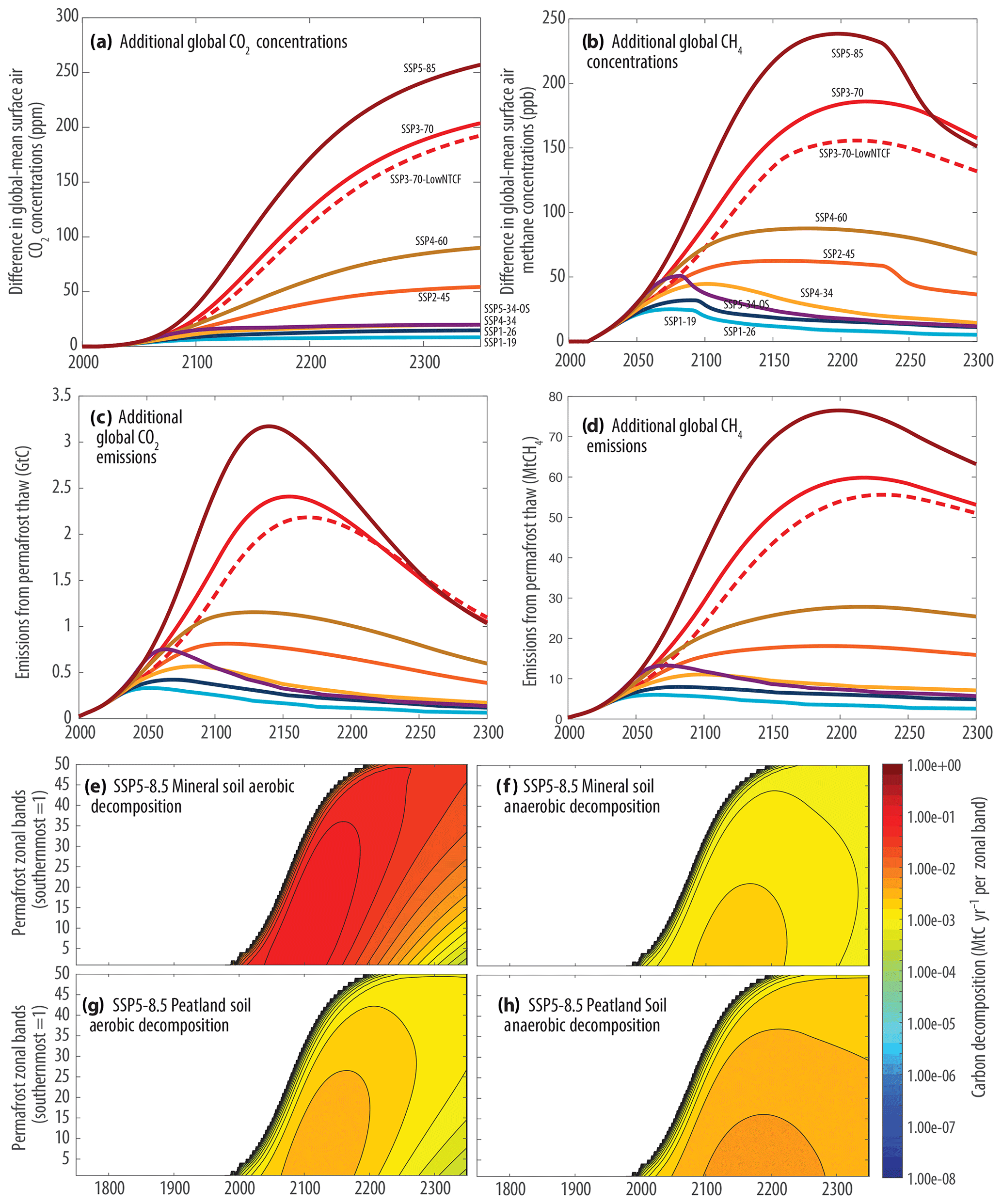
Figure 3 The assumed permafrost-related emissions by using MAGICC's permafrost module in its default settings for the SSP GHG concentration projections, close to the median of the probabilistic MAGICC permafrost version (Schneider von Deimling et al., 2012). In the highest scenario, SSP5-8.5, CO₂ and CH₄ concentrations by 2300 would have been about 250 ppm and 150 ppb, respectively, lower without including the permafrost module (a, b). The additional CO₂ from mineral soil and peatland carbon decomposition reach a maximum in the highest scenario SSP5-8.5 around 2140 of about 3 GtC emissions per year (c), mainly due to the aerobic mineral soil decomposition (e). The mineral and peatland soil decomposition under aerobic conditions (e and g, respectively) and also the oxidized part of the methane that originates from the anaerobic decomposition (f, h) contribute to the net CO₂ emissions from permafrost thawing. The permafrost zonal bands are a simplified approach to represent the range of thawing thresholds and permafrost carbon contents and are described in Schneider von Deimling et al. (2012). See Table 2 for cumulative emissions.

Table 2 Cumulative CO₂ and CH₄ emissions from MAGICC's permafrost module under the considered SSPs. The permafrost module has 50 zonal bands, a mineral and peatland soil module, and 50 latitudinal zonal bands. See Schneider von Deimling et al. (2012) for a detailed description. See Fig. 3 for time series of induced CO₂ and CH₄ atmospheric concentration changes.

In addition to elevated CO₂ concentrations, the permafrost module also estimates future CH₄ emissions related to permafrost thawing, i.e. annual emissions of up to 75 MtCH₄ yr⁻¹ in the highest SSP5-8.5 scenario by 2200. Cumulatively, 0.34 to 1.07 GtC of carbon are projected to be released as 451 to 1431 MtCH₄ over the course of the 21st century across the nine considered SSP scenarios (Table 2), with even more coming in the 22nd century. The extra emissions lead to 10–240 ppb higher CH₄ concentrations in 2200 (Fig. 3b). Most of the carbon decomposition is assumed to happen as aerobic decomposition in the mineral soils, stretching from the more southerly zonal permafrost bands to the higher latitudes from now to 2200 (Fig. 3e to h).

2.5 Projecting latitudinal gradients

Compared to the previous input datasets for CMIP intercomparisons, which consisted of global-mean values only, latitudinal gradients (and seasonality) are new elements. For the historical period, these latitudinal gradients and seasonally changing surface air concentrations can be estimated from the large set of in situ and flask sampling sites with a monthly sampling resolution. Further back in time, when there was insufficient latitudinal coverage, the latitudinal gradient was decomposed into two empirical orthogonal functions (EOFs, the principal components). The multiplier or score (also known as the principal component time series) for the first EOF was regressed against global anthropogenic emissions. Except for CO₂, the score for the second EOF was kept constant. For CO₂, we assumed a simplified approach by both assuming a zero intercept for the regression of global emissions versus the first EOF and a phase-out back in time of the second EOF score. These lead to the simplified and uncertain assumption that the pre-industrial CO₂ gradient was zero (Fig. 9b in Meinshausen et al., 2017). For a more detailed description of the interpolation and assimilation algorithms for the historical data, see Meinshausen et al. (2017).

For the future, there are obviously no observations from which the changes in the latitudinal gradients can be derived. We hence apply the regression procedure from the historical dataset into the future, i.e. we project the score of the first EOF of the latitudinal gradient of each greenhouse gas with its global emissions. That makes the simplifying assumption that, in the future, the sources (and sinks) of these gases remain approximately constant in terms of their latitudinal location (not in terms of their magnitude). For CO₂ in the very low emission scenarios, like SSP1-1.9 with net negative CO₂ emissions, that leads to a plausible reversal of the latitudinal gradient if the Northern Hemisphere is the main location for the natural and anthropogenically induced net CO₂ sink.

There are large natural CH₄ emission sources, predominantly in the Northern Hemisphere. Also, anthropogenic emissions are higher in the Northern Hemisphere. This largely explains the observed atmospheric concentration gradient: At the end of the historical period (2010 to 2014), CH₄ concentrations are 80 ppb above the global average in the northern midlatitudes while southern hemispheric concentrations gently slope towards a minimum of 60 ppb below the global average at the pole (Fig. 11b in Meinshausen et al., 2017). As for CO₂, we use anthropogenic CH₄ emissions to extrapolate the first EOF score into the future. Given that CH₄ emissions do not converge to zero in any scenario, let alone become negative, the strong north–south gradient is maintained in all scenarios.

2.6 Projecting seasonality

Seasonality of concentrations is by far most strongly pronounced for CO₂, given the large seasonal sink (photosynthesis) and source (heterotrophic respiration) pattern of the northern hemispheric terrestrial biomass. Projecting future seasonality changes depends on a correct understanding of the past seasonality changes and how those seasonality changes are related to changes in ecosystem productivity (Forkel et al., 2016; Graven et al., 2013; Welp et al., 2016), increased cropland productivity (Gray et al., 2014), and other factors. Here, we use the net primary productivity (NPP) as a proxy for future seasonality changes and regress the historically derived seasonality change EOF score with modelled future net ecosystem exchange by MAGICC7. NPP in MAGICC7 is projected to increase strongly in the highest SSP5-8.5 scenario, while following a maximum-then-decline pattern in the lower SSP1-1.9 scenario. At the end of the historical period, the total seasonality is derived to have a minimum concentration deviation of −10.1 ppm in northern midlatitude August. Given these projected NPP changes in the high SSP5-8.5 scenario, the projected total seasonality increases to approximately twice that by 2100, a projection that comes with a high degree of uncertainty.

For all other gases for which we identified a significant seasonal cycle in the historical observational data, we assume that the relative seasonality (i.e. the magnitude of monthly anomalies relative to the annual mean) stays constant, i.e. that the absolute seasonality concentration changes scale with global-mean concentrations.

2.7 Simplified formula to reflect radiative forcing from CO₂, CH₄, and N₂O

In order to present CO₂, CH₄, and N₂O in our compilation of 43 greenhouse gases and their relative importance for future effective radiative forcings (ERFs), we use simplified radiative forcing formulas (for radiative forcing after stratospheric temperature adjustments) that represent the Oslo Line-By-Line model results – which now take into account the short-wave absorption of CH₄, among other aspects (Etminan et al., 2016). While Etminan et al. (2016) provided simplified formulas for their Oslo Line-By-Line model results, we here adjust those simplified formulas, resulting in a virtual elimination of the model fit errors by Etminan of up to 3.6 % for CO₂ (see Table 1 in Etminan et al., 2016, and our Fig. 4d and Table 3 below). Aside from slight model misfits, the original Etminan simplified formula for CO₂ has a validity range of only up to 2000 ppm CO₂ concentrations. Their simplified formula is an adaptation of the classical approach to approximate radiative forcing by $\mathit{\alpha }\times \ln \left(\frac{C}{C_{\mathrm{0}}}\right)$, where α is a scaling coefficient, C the CO₂ concentration at time t and C₀ the concentration at the reference state, normally the pre-industrial reference value. Etminan et al. introduce the overlap of the absorption spectra between CO₂ and N₂O and also modulate the logarithmic approximation by quadratic and linear terms. When using their suggested coefficients (a₁, b₁, and c₁ in their Table 1), the factor α in front of the $\ln \left(\frac{C}{C_{\mathrm{0}}}\right)$ part reaches a maximum at $C_{\mathrm{0}}-\frac{b_{\mathrm{1}}}{\mathrm{2}{a}_{\mathrm{1}}}$, i.e. at around 1777 ppm, when assuming C₀ as the pre-industrial concentration (277.15 ppm). For CO₂ concentrations beyond 1777 ppm, the alpha value decreases, leading to an unrealistic flattening off above 2000 ppm (and eventual decline well above 3000 ppm). The highest projected SSP concentration (SSP5-8.5) reaches beyond the nominated validity range of 2000 ppm. Hence, we adapt the CO₂ radiative forcing formula to assume a constant α, once α reaches its maximal value (which is around 1808 ppm with our optimized parameter settings – see Table 3).

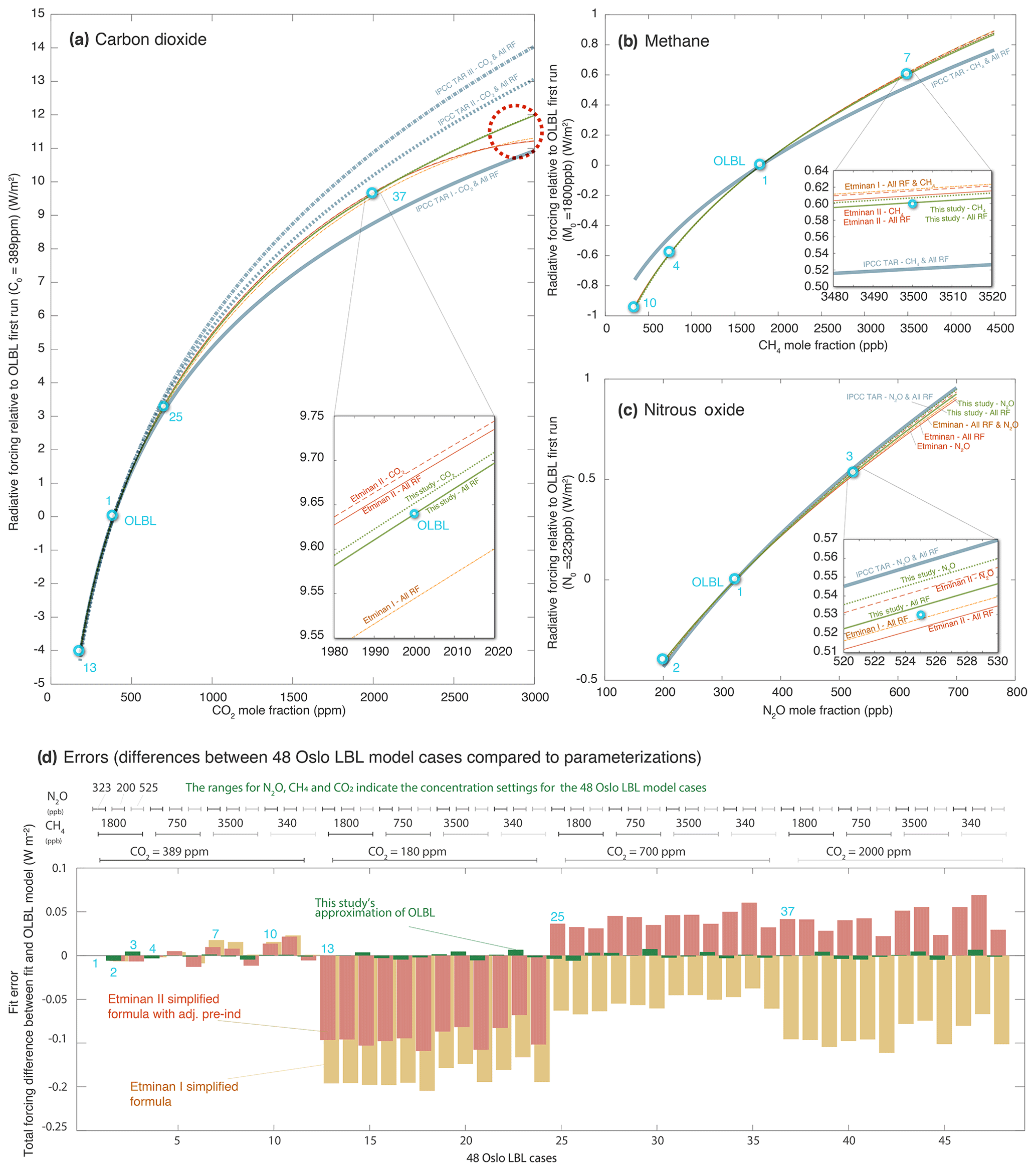
Figure 4 Simplified parameterization to emulate 48 Oslo Line-By-Line model results (bright blue open numbered circles). Shown are the IPCC TAR simplified formula for CO₂ (three options), CH₄, and N₂O forcing with their default parameter settings (grey-blue lines) in the background. The simplified formula results by Etminan et al. (2016) are shown as orange lines. Adjusting pre-industrial concentration values to default 1750 values improves the fit of the Etminan simplified formula (red lines in panels a to c and red error terms in panel d). This study's simplified formula results are shown in green, matching the Oslo Line-By-Line model results within rounding – and continuing a forcing approximation beyond 2000 ppm CO₂ in line with previously derived formulas (red dashed circle in panel a). See text.

Table 3 Simplified expressions for radiative forcing relative to pre-industrial (1750) levels by changes in surface air mole fractions of CO₂, CH₄, N₂O – reflecting the Oslo Line-by-Line model results. This table can be compared to Table 1 in Etminan et al. (2016), but note that their formulas can be directly applied to any sets of (C, Co), (M, Mo), and (N, No) within the range of fitting, unlike the case here where Co, Mo, and No are pre-specified at pre-industrial levels.

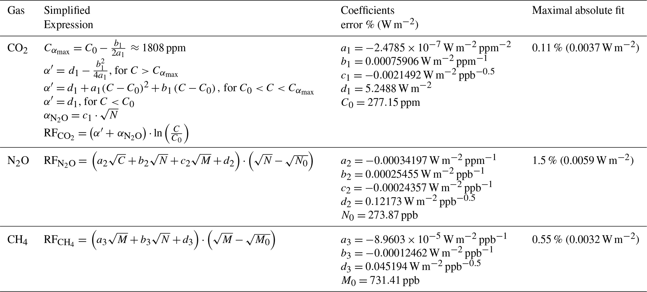
In summary, building on the work of Etminan, our optimized modifications of the simplified radiative forcing expressions for CO₂, CH₄, and N₂O as presented in Table 3 have the two advantages of (a) representing the 48 Oslo Line-By-Line model results within rounding errors and also (b) extending its likely validity range in line with previous forcing approximations (and pending examinations by Line-By-Line models) to higher CO₂ concentrations. However, there is one disadvantage of our simplified formula. While our formula starts from fixed C₀, N₀, and M₀ values at pre-industrial levels, the formulas presented in Etminan cater for the option to set C₀, N₀ and M₀ at any value within the validity range. Hence, our formula would have to be applied twice to calculate the difference in terms of radiative forcing between a C₁, N₁, M₁ and a C₂, N₂, M₂ concentration state if both are different from pre-industrial levels C₀, N₀, and M₀.

We also take into account new findings regarding rapid adjustments (Smith et al., 2018). In the multi-model analysis by Smith et al. (2018), CO₂ is suggested to have a slightly (∼5 %) higher effective radiative forcing than its instantaneous radiative forcing after stratospheric temperature adjustments alone, an adjustment also used here. While the tropospheric rapid adjustments in the case of CO₂ is substantial, it is largely offset by the corresponding water vapour adjustment and the cloud-related rapid adjustments (Fig. 3 in Smith et al., 2018). Following Smith et al. (2018), we assume that rapid adjustments largely cancel out for CH₄.

2.8 Data-flow, mean-preserving higher resolutions, and merging with historical files

In this study's projections, the data is provided in 15^∘ latitudinal bands with monthly resolution. These are constructed from the global-mean time series generated by MAGICC7, with the modulation towards latitudinal annual means by the time-changing latitudinal gradients (Sect. 2.5). These latitudinal annual means are then turned into monthly data values using the latitudinally and monthly resolved seasonality fields.

There are two additional post-processing steps involved. For one, the mean-preserving interpolation routines from Sect. 2.1.9 of Meinshausen et al. (2017) are used to generate a monthly surface air mole fraction field at a finer 0.5^∘ latitudinal resolution. The other step is merging the projections with the historical concentrations. To ensure a smooth transition from the previously derived historical concentration fields to the ones derived in this study, we use the latitudinally resolved differences in the month of December 2014 between the historical fields derived in Meinshausen et al. (2017) and the raw data produced here. We then add those December 2014 differences to the 2015 future datasets, phasing them out linearly over 12 months.

3 Results

This study's projected greenhouse gas concentrations provide the “official” greenhouse gas concentrations for the SSP scenarios. They help enable the CMIP6 exercises and span a wide range of possible futures. Below, the results are presented for the various gases. The complete data repository of all projected mole fractions in various data formats, with interactive plots and fact sheets is available at http://greenhousegases.science.unimelb.edu.au (last access: 20 June 2020). The subset of the data recommended for the nine SSPs that are part of the ScenarioMIP and AerChemMIP experiments in netcdf format is also available on https://esgf-node.llnl.gov/search/input4mips/ (last access: 20 June 2020).

3.1 Carbon dioxide

The projected CO₂ concentrations range from 393 to 1135 ppm in 2100, with the low scenario SSP1-1.9 decreasing to 350 ppm by 2150 (Fig. 5g). Given the assumption of zero CO₂ emissions in the lower scenarios beyond that, the lower end of the projected CO₂ concentrations is not projected to decrease much further. On the upper end, under the SSP5-8.5 scenario global-average concentrations are projected to increase up to 2200 ppm by 2250 (Tables 4 and 5, and see also online “GHG fact sheets” at http://greenhousegases.science.unimelb.edu.au). The latitudinal gradient implies a difference of annual-average northern midlatitudes to South Pole concentrations of about 6 ppm in current times (Fig. 5b). As future seasonality is correlated with projected NPP, the CO₂ seasonality change pattern (Fig. 5a.1) is scaled with the a normalized projected NPP (Fig. 5a.2). Future latitudinal gradients are derived by projecting the first two principal components or EOFs, where the first (dark-blue line in Fig. 5c) is regressed against global emissions – with the implied future scaling factor show in Fig. 5d (dark-blue line). The second EOF (turquoise line in Fig. 5c) is assumed to be constant in the future (turquoise line in Fig. 5d). The applied projection methods result in a continuous projection of CO₂ concentration from the observationally derived historical values, including their latitudinal gradients and seasonality (Fig. 5h). By approximately 2060, a zero latitudinal gradient is projected in the lowest SSP1-1.9 scenario (Fig. 5b) because CO₂ emissions revert from positive to net negative. Under the highest SSP5-8.5 scenario, the northern midlatitude to South Pole difference expands to more than 23 ppm by 2100 (not shown in plot, but viewable in online data repository at http://greenhousegases.science.unimelb.edu.au).

Table 4 Overview of future scenario range of individual GHG concentrations. The table indicates the minimum and maximum surface air mole fractions across the nine SSP scenarios considered in this study. For spreadsheets with annual data tables per scenario, see http://greenhousegases.science.unimelb.edu.au. The third column indicates the region, with global (“GL”), northern hemispheric (“NL”) and southern hemispheric (“SH”) data shown for CO₂, CH₄ and N₂O. The last three rows provide the equivalence concentrations. The CFC-11-eq concentrations summarize – in terms of radiative forcing equivalent – all greenhouse gases aside from CO₂, CH₄, N₂O, and CFC-12. The CFC-12-eq concentrations summarize all the ozone-depleting substances (ODSs) controlled under the Montreal Protocol, while HFC-134a-eq summarizes the remaining fluorinated gases. Altogether CO₂, CH₄, N₂O, CFC-12-eq, and HFC-134a-eq together represent the radiative forcing of the entirety of the 43 greenhouse gases considered here (cf. Table 5 in Meinshausen et al., 2017).

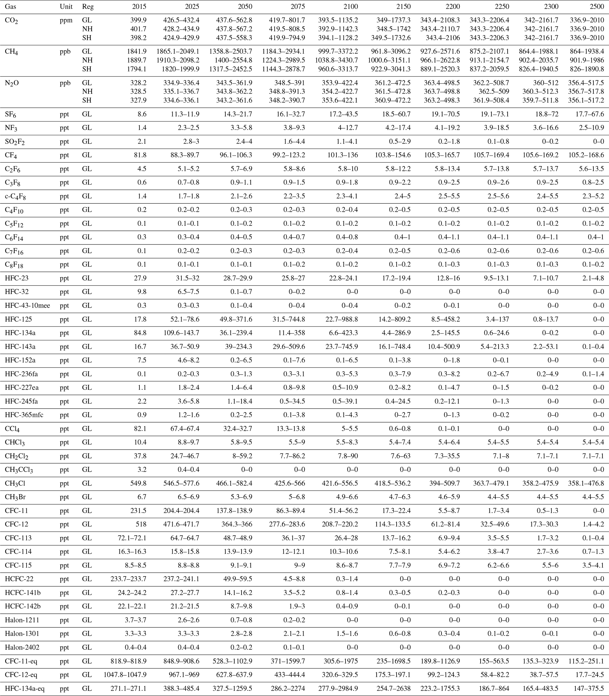
Table 5 Overview of CO₂ CH₄ and N₂O concentrations in the eight SSP scenarios considered in this study with global-average (“GL”) northern hemispheric (“NH”) and southern hemispheric (“SH”) surface air mole fractions. For annual and latitudinally resolved mole fractions and other greenhouse gases see the Supplement or http://greenhousegases.science.unimelb.edu.au.

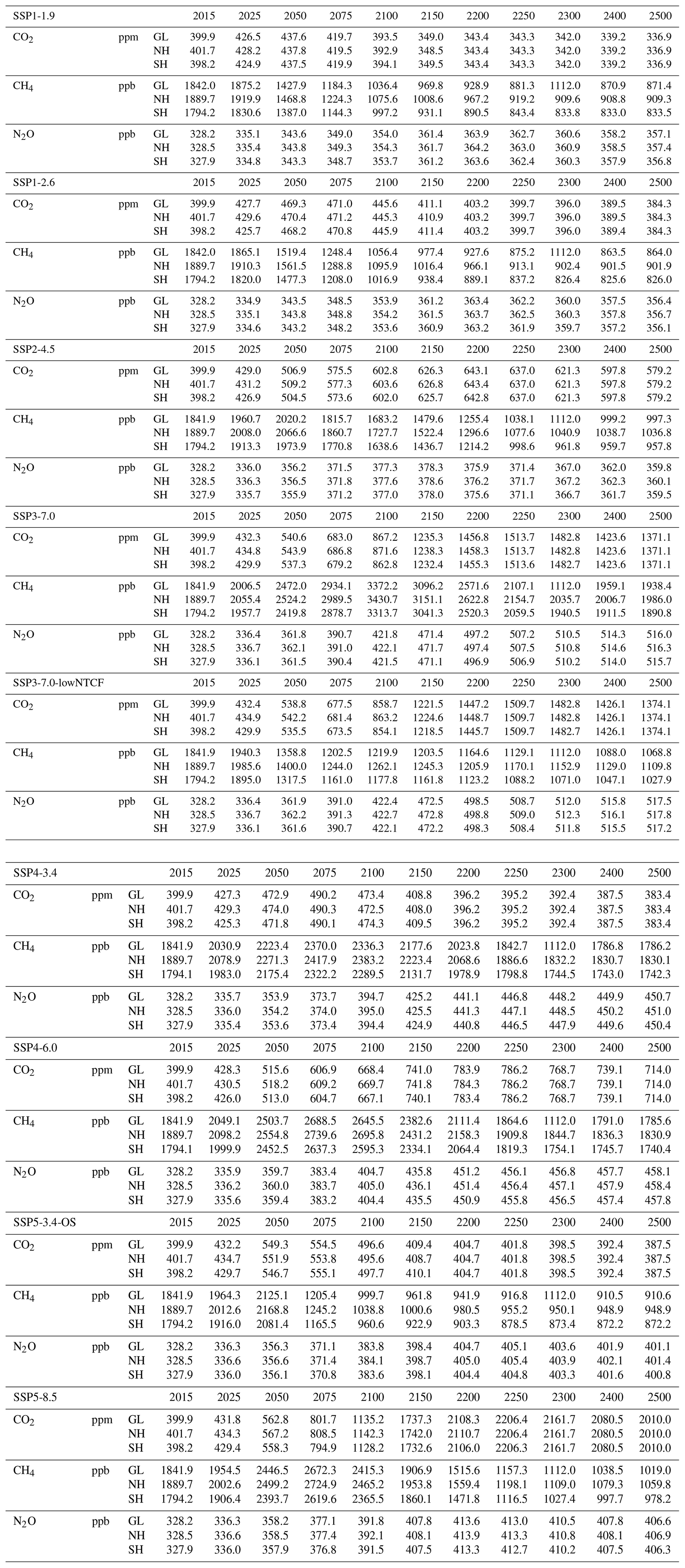
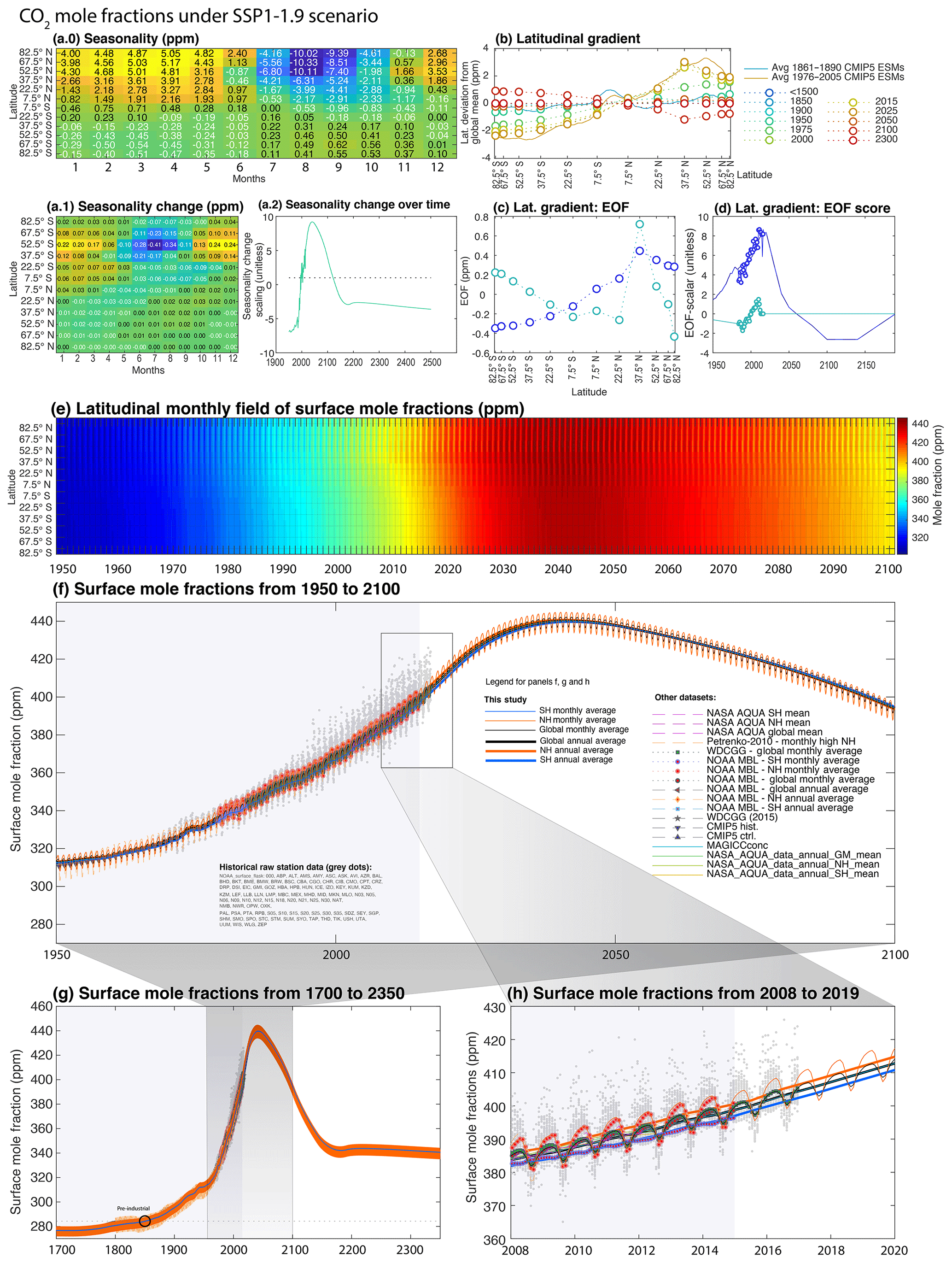
Figure 5 CO₂ concentrations under the SSP1-1.9 scenario. The base seasonality pattern derived from historical observations with monthly and 15^∘ latitudinal resolution (a) is modulated over time using the first EOF of the residuals (a.1), scaled with projected NPP into the future (a.2). The latitudinal gradient is assumed to be flat in pre-industrial times, with latitudinal gradients over the observational record being derived from historical observations – and here compared with CMIP5 ESM models – see Meinshausen et al. (2017) (b). The projection of the latitudinal gradient uses global total CO₂ emissions regressed against the score (dark-blue line in panel d) of the first latitudinal EOF (dark-blue line in panel c). The principal component's score of the second EOF's is assumed to be zero in the future (turquoise line in panel c, d). Resulting surface air mole fractions fields show a return to current CO₂ (∼2019) concentrations by the end of the 21st century (e, f). Historical NOAA surface flask station datasets (grey dots in panels f, g, h with station indicators provided in legend of panel f) are used for these future projections beyond the end of 2014 reach of the historical dataset (grey shaded background in panels f, g, h). Various comparison datasets shown, namely the WDCGG time series (Tsutsumi et al., 2009), the NOAA Marine Boundary Layer (MBL) product (https://www.esrl.noaa.gov/gmd/ccgg/mbl/, last access: 20 June 2020) and the NASA AQUA satellite data (ftp://acdisc.gsfc.nasa.gov/ftp/data/s4pa/Aqua_AIRS_Level3/AIRX3C2M.005/, last access: 20 June 2020), the Petrenko time series (made available in the Supplement to Buizert et al., 2012). Also shown are the MAGICC global-mean projections (bright blue line “MAGICCconc”). These overview figures are available for all 43 gases and all nine scenarios on http://greenhousegases.science.unimelb.edu.au as a total of 387 so-called fact sheets. See also Table 12 in Meinshausen et al. (2017) for a description of all data labels.

3.2 Methane

Global-mean CH₄ surface air mole fractions across the SSP scenarios are projected to range from 999.7 to 3372 ppb by 2100, with maximal northern hemispheric averages being ∼60 ppb higher than the global average (Table 4). The largest difference between average northern and southern hemispheric concentrations (up to 120 ppb by 2100, Table 5) is in the highest CH₄ emissions scenario (SSP3-7.0) and whilst the smallest difference (∼70 ppb) is seen in the scenarios with the lowest global CH₄ emissions (SSP1-1.9, SSP1-2.6, and SSP5-3.4OS). While SSP5-8.5 is projected to be the scenario with the highest radiative forcing because of high CO₂ emissions, SSP5-8.5 is not the highest CH₄ emissions scenario, with both SSP3-7.0 and SSP4-6.0 suggesting higher total CH₄ emission by 2100 (and in our extensions beyond 2100) (Fig. 2f).

3.3 Nitrous oxide

N₂O concentrations are not projected to decrease at any point before 2200, regardless of the SSP scenario we consider. Even under the lowest emissions scenarios, SSP1-1.9 and SSP1-2.6, current global-average concentrations are projected to increase from 328.5 ppb in 2015 to 361 ppb by 2100 (Table 5). Under the highest N₂O scenarios (SSP3-7.0 and SSP3-7.0-lowNTCF), concentrations are projected to increase to 422 ppb by 2100 and over 500 ppb by 2500. Both seasonality and the latitudinal gradient is rather subdued for N₂O, as it is both a long-lived greenhouse gas and does not exhibit strong seasonal variability in either sources or sinks.

3.4 Ozone-depleting substances and other chlorinated substances

As all ozone-depleting substances' emissions are assumed to follow a single emission scenario as a result of the Montreal Protocol (Velders and Daniel, 2014), the SSP concentration scenarios exhibit no substantial variation across their projected concentrations. For example, by 2100, CFC-11 and CFC-12 concentrations are assumed to vary from 51.4 to 56.2 ppt, and from 114.3 to 133.5 ppt, respectively (Table 4). These differences across the concentration scenarios are hence not a result of different emission assumptions but solely due to factors that influence the substances' lifetimes. The stratospheric partial lifetime of these substances is affected by a change in the meridional Brewer–Dobson circulation, assumed to strengthen with increasing climate forcing. The tropospheric OH-related partial lifetime is scaled by changing OH concentrations. Those OH concentrations are in turn mainly affected by CH₄ abundances and emissions of other reactive gases (CO, NMVOC, NO_x). Overall, the concentrations and radiative forcing contributions of all ozone-depleting substances are assumed to strongly reduce until 2100 and beyond, following the phase-out schedules under the Montreal Protocol (Fig. 10). See Sect. 4.2 for a discussion of the unexpectedly slow declines of CFC-11 (Montzka et al., 2018) and other species, though.

3.5 Other fluorinated greenhouse gases

Emissions of fluorinated gases with a virtually zero ozone-depleting potential – HFCs, PFCs, SF₆, and NF₃ – vary across the SSP scenarios. Most SSP scenarios assume strong decreases for several of these substances (e.g. NF₃ and SF₆), while SSP5-8.5 assumes strong increases for most of the 21st century (Fig. 2h, i). Until recently, these fluorinated gases were not controlled under the Montreal Protocol. With the 2016 Kigali Amendment, however, a select number of HFCs have been included in the Montreal Protocol and GWP-weighted emissions of these particular HFCs will have to be phased-down globally in coming decades. When aggregating all these non-ozone-depleting fluorinated gases into HFC-134a equivalent concentrations, the SSP scenarios project a wide range of 2100 values, ranging from 278 ppt to more than 10-fold that value, i.e. 2985 ppt (last row in Table 4). While the HFC projections are derived from the IAM modelling team assumptions regarding the SSPs, several of the resulting HFC projections would exceed the phase-out emission levels agreed to in the Kigali Agreement.

3.6 Radiative forcing since 1750

In this section, we aggregate all 43 greenhouse gases' radiative forcing effect using the updated radiative forcing formula for CO₂, CH₄, and N₂O and standard radiative efficiencies from IPCC AR5 (Sect. 2.7). Across the nine SSP scenarios, it is apparent that CO₂ makes the largest contribution to future warming (blue parts in Fig. 7), constituting between 68 % and 85 % of GHG radiative forcing by 2100, and 68 % to 92 % of radiative forcing by the time of maximum GHG-induced radiative forcing (Table 6). In the scenario with the greatest radiative forcing, SSP5-8.5, radiative forcing in 2100 is projected to be approximately 8 and 9.7 W m⁻² for CO₂ or all GHGs, respectively (right-axis bars in Fig. 7i). This greenhouse-gas-induced radiative forcing is projected to increase to nearly 13 W m⁻² by 2250 under SSP5-8.5. On the lower side, the SSP1-1.9 scenario exhibits a CO₂ radiative forcing of around 1 W m⁻² in 2150 and beyond, with total greenhouse-gas-induced forcing stabilizing around 1.5 W m⁻² – equivalent to CO₂ concentrations of approximately 370 ppm (right axis in panel a of Fig. 7).

Table 6 Fraction of greenhouse-gas-induced forcing due to CO₂ concentrations in SSP scenarios at the point of maximal greenhouse-gas-induced forcing until 2300 (upper row) or in the year 2100 (lower row).

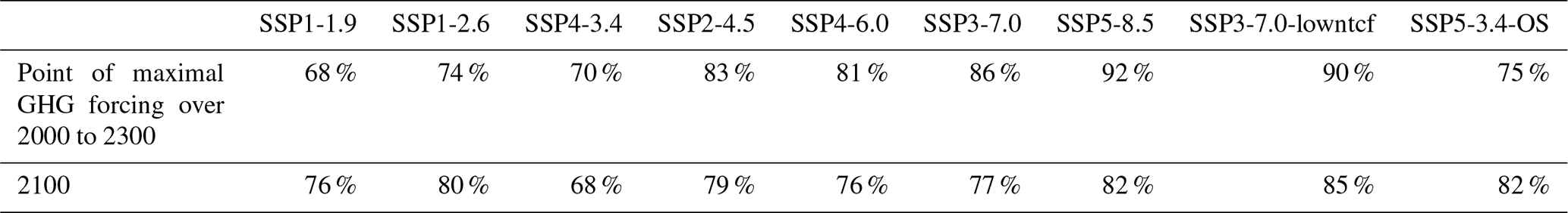
Table 7 SSP global mean surface air temperature (GMSAT) and global mean sea level rise (GMSLR) projections for the end of the 21st century (2081–2100 average and 2100 estimate) and 2300. GMSAT is shown in kelvin relative to 1750; GMSLR is shown in metres relative to the 1986–2005 average. Mean and 5th to 95th percentiles are provided for both variables.

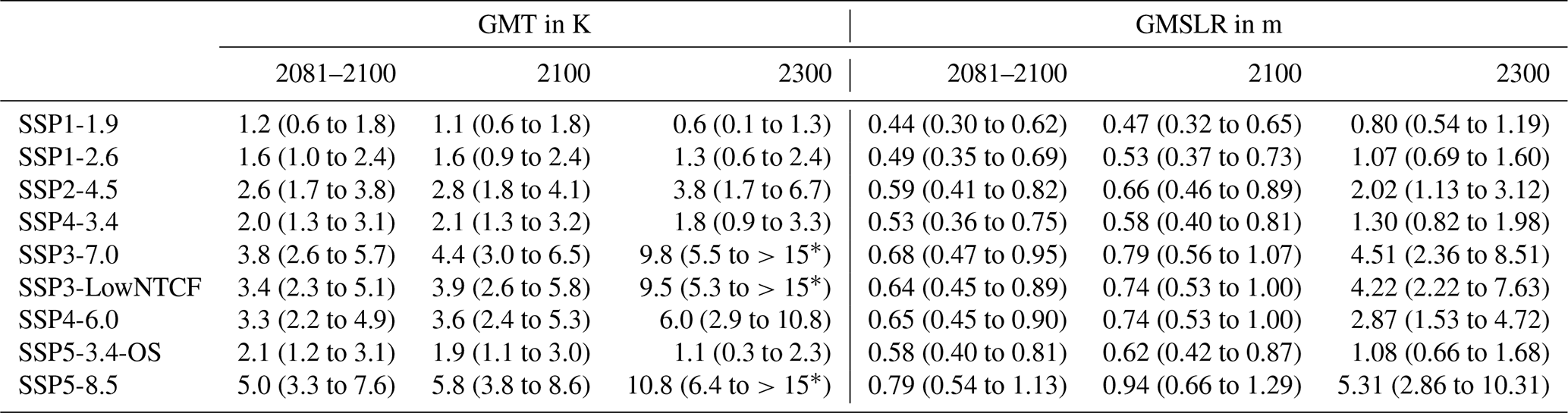
^* MAGICC has an internal cutoff temperature in each land–ocean and hemispheric box at 25 K. Any temperatures indications beyond 10 K should be considered illustrative
only given that the calibrated range of MAGICC covers only lower temperature levels.

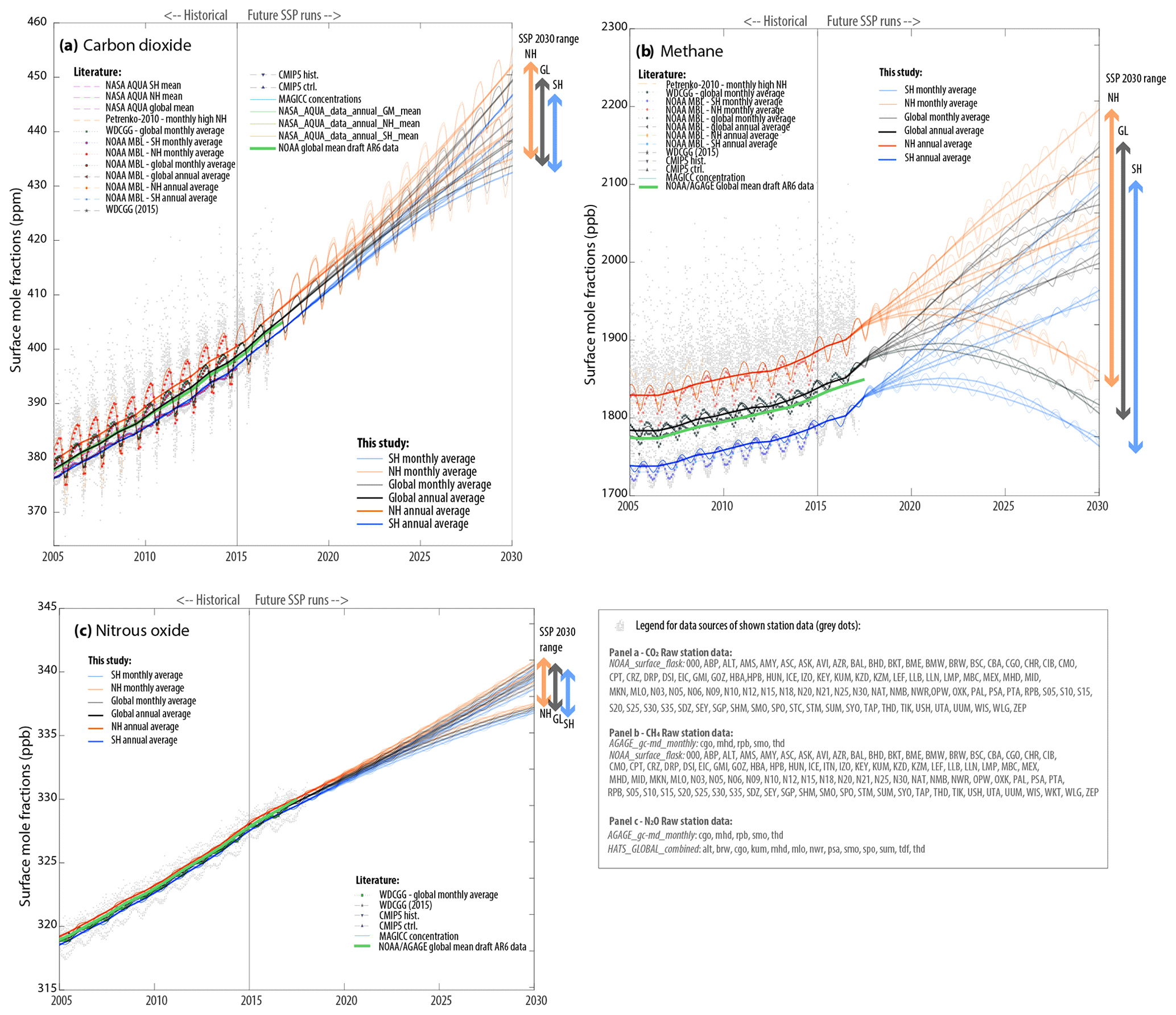
Figure 6 Transition between historical runs and future SSP concentrations for CO₂ (a), CH₄ (b), and N₂O (c) surface mole fractions. The observational in situ and flask station data points reach into the first years of the future SSP datasets (grey dots). Derived northern hemispheric (orange), global (black), and southern hemispheric averages (blue) are shown with annual averages (thick lines) and monthly averages (thin lines with seasonality variability). On the right axis side, the illustrative arrows indicate the min–max range across the scenarios for northern hemispheric, global, and southern hemispheric annual-average concentrations by 2030 across all nine SSP scenarios. The NOAA/AGAGE global mean data series are shown in green. For a description of labels of other comparison data, see Table 12 in Meinshausen et al. (2017).

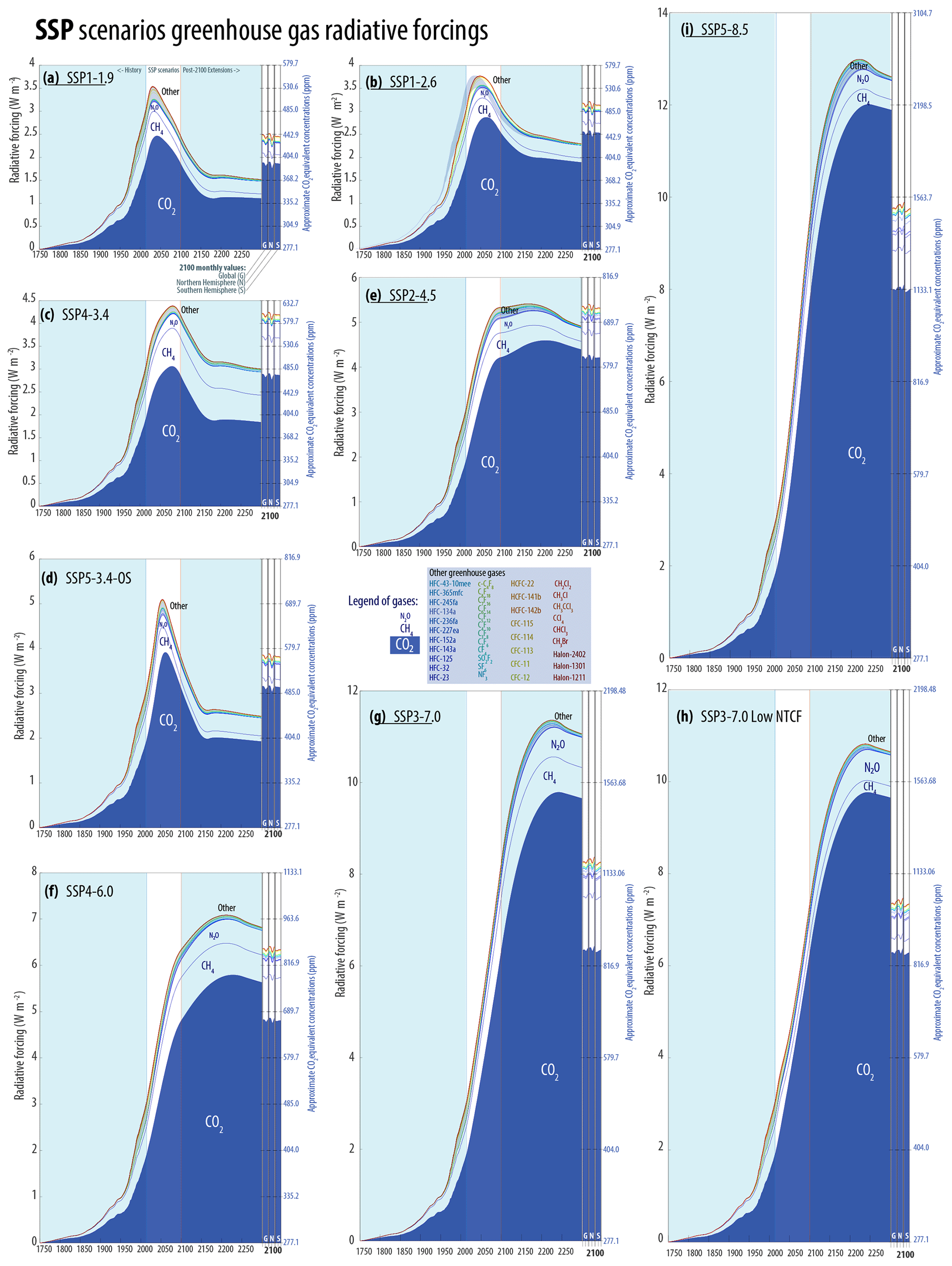
Figure 7 Overview of all greenhouse gases within SSP scenarios and their relative importance in terms of radiative forcing. The radiative forcing contributions are stacked, starting with CO₂ (blue shaded area) at the bottom, followed by methane (CH₄), nitrous oxide (N₂O), and the other 40 greenhouse gases. Default radiative forcing efficiencies or parameterizations are used, with CO₂, CH₄, and N₂O being based on a parameterization of the Oslo Line-By-Line model (Sect. 2.7). Seasonal and latitudinal variation is indicated by the three bars on the right of each panel for the global average, northern hemispheric, and southern hemispheric monthly mean concentrations for the year 2100. The light-blue shaded areas on the left side of each panel from 1750 to 2014 are based on historical greenhouse gas observations; the 21st-century span from 2015 to 2100 (white area) and the extension until 2300 and beyond are based on the MAGICC7.0 model. For the IPCC AR6, the five scenarios SSP1-1.9 (a), SSP1-2.6 (b), SSP2-4.5 (d), SSP3-7.0 (g), and SSP5-8.5 (i) are chosen as key scenarios for knowledge integration across chapters and working groups.

4 Discussion

In this section, we discuss the SSP greenhouse gas concentration projections in relation to the last 2000 years of observations and cumulative carbon emissions, which are an important metric for mitigation efforts. We also provide a comparison to previous RCP pathways.

4.1 CO₂ and CH₄ concentrations

After CO₂, the greenhouse gas with the second largest radiative forcing contribution in the 21st century is CH₄ (Fig. 7). To a large extent, greenhouse gas induced future warming is hence influenced by the concentrations of CO₂ and CH₄. Two examples in which methane and CO₂ forcings and their relative strength are important. (i) Firstly, discussions about the benefit of the mitigation of short-lived forcers often accounts for CH₄ as a short-lived forcer, which usually contributes most of the climate benefits of any short-lived forcer mitigation strategy (Rogelj et al., 2015, 2014). Hence, when the climate benefits of reducing short-lived forcers are compared to those of reducing CO₂ emissions, the actual comparison is mostly between CH₄ and CO₂. Secondly, deriving the remaining carbon budget from Earth system model runs from single or a few scenario runs is contingent on those scenarios showing a representative level of CH₄ versus CO₂ concentrations. Here, we consider mid-21st-century CH₄ and CO₂ concentrations across the range of SSP scenarios. We place them in the context of the RCP scenarios as well as 475 scenarios of the IPCC Special Report on 1.5 ^∘C emissions database (https://data.ene.iiasa.ac.at/iamc-1.5c-explorer/, last access: 20 June 2020) (Fig. 9). We focus on mid-century concentrations as they are close to the expected point of peak warming in the scenarios that are in line with the Paris Agreement temperature targets of 1.5 ^∘C and well below 2.0 ^∘C. The comparison shows that SSP1-1.9 and SSP1-2.6 result in relatively similar CH₄ concentrations by 2050, albeit their CO₂ concentrations differ by approximately 7 % (437 ppm versus 469 ppm, respectively, Table 5). The other scenario with low CH₄ concentrations in 2050, i.e. SSP3-7.0-lowNTCF, falls outside the scenario space considered here, namely the SR.15 database (https://data.ene.iiasa.ac.at/iamc-1.5c-explorer/, see Fig. 9 below). This is by design, as this scenario is the result of adapting a high-emission scenario (SSP3-7.0) so that it features very low short-lived climate forcer emissions (Collins et al., 2017). See also Appendix C in Gidden et al. (2019) for a detailed comparison of SSP3-7.0 and SSP3-7.0-lowNTCF emissions. The comparison of mid-century CO₂ and CH₄ concentrations also reveals that the main reason for higher implied warming of SSP4-3.4 in comparison to SSP1-2.6 are elevated CH₄ concentrations. Thus, to a limited extent, the SSP4-3.4 and SSP1.2.6 scenarios represent a similar pair of scenarios to the SSP3-7.0 and SSP3-7.0-lowNTCF scenarios, but for a lower level of cumulative CO₂ emissions.

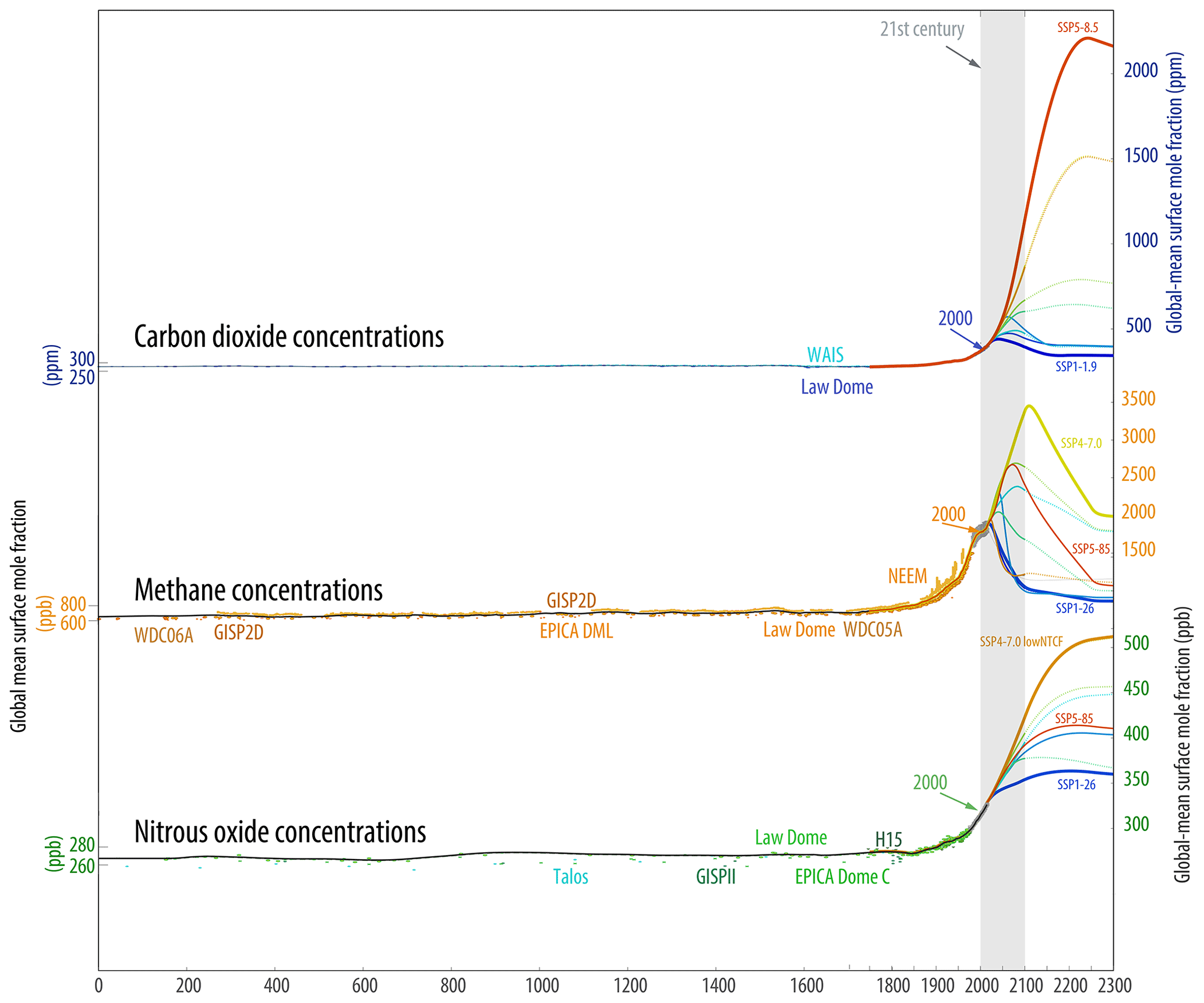
Figure 8 Overview of SSP concentrations of CO₂, CH₄, and N₂O in the context of the historical observational dataset. For the respective main ice core and firn datasets (WAIS, Law Dome, EPICA DML, etc.), please see Fig. 6b in Meinshausen et al. (2017). The 21st century is shown as a grey vertical band.

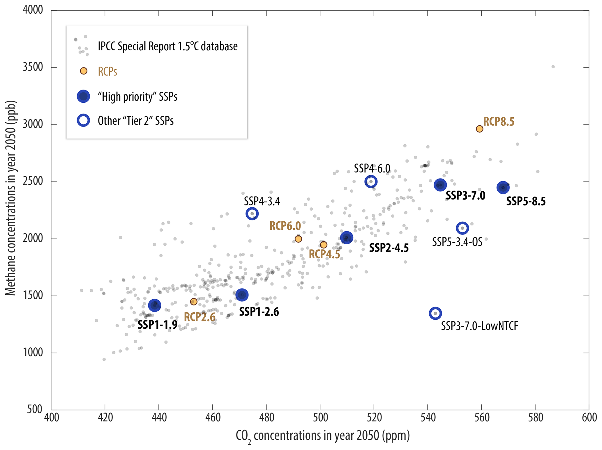
Figure 9 The 2050 CO₂ and CH₄ concentrations of SSPs (dark-blue circles), RCP (orange circles), and scenarios of the IPCC Special Report on 1.5 ^∘C warming database (grey dots). All scenarios' concentrations were derived by using the SSP or RCP or SR1.5 harmonized emission scenarios together with the same MAGICC7.0 default settings as used for the CMIP6 SSP concentration projections.

4.2 Most recent concentration observations

While updating the historical observations for our future concentrations, several recent trends are noteworthy. We discuss these in this section, covering CH₄, ozone-depleting substances CFC-11, CFC-12, CFC-113 as well as HFC-23 and SF₆.

Regarding CH₄, atmospheric observations show a plateauing of CH₄ concentrations from 1999 to 2005 followed by an increased growth rate from 2007 (Nisbet et al., 2016). Available literature suggests that changes in natural and anthropogenic sources and OH-related sinks are involved (Rigby et al., 2017), for example reduced biomass burning emissions (Worden et al., 2017) or reduced thermogenic fossil-fuel-related emissions (Schaefer et al., 2016) to explain the plateau of concentrations until 2006, but large uncertainties remain, particularly related to natural wetland and inland water sources (Saunois et al., 2016). Schaefer et al. (2016) suggest that the renewed onset of increasing CH₄ concentrations could be related to increased emissions from the agricultural sector.

Our CH₄ concentration time series, both the historical ones and the future projections from 2015 onwards, capture this observed increase in the trend Fig. 6b) – although there is uncertainty as to whether the underlying processes and emission sources are correct. Nevertheless, our employed simple model MAGICC7 also captures this temporary plateau of CH₄ concentrations when run in an emission-driven model, possibly not the earlier parts though (left column in Supplement Fig. S1). Note that the transition in 2017 from observationally driven concentrations to our model-driven concentration time series exhibits a slight offset in concentrations (Sect. 5.3), as MAGICC7 inferred a slightly stronger increase in CH₄ concentrations over 2016 based on the IAM's emissions, than observed (Fig. 6).

For nitrous oxide, there appears to be a small downward adjustment in the growth rate around 2014, with atmospheric growth in the years 2016 and 2017 being slightly lower than in 2014 (Fig. 6c), although observed 2018 growth rates picked up again and the slight offset seems to be well within the noise of recent growth rate variations. For a close comparison of recent observations and our concentration time series, see the CH₄- and nitrous oxide-related fact sheets at http://greenhousegases.science.unimelb.edu.au.

Recent observations regarding substances whose production is largely phased out under the Montreal Protocol are also notable (Montzka et al., 2018; Rigby et al., 2019). CFC-11 measurements show some elevated Northern Hemisphere values from 2013 onward and the global average concentrations are 5–10 ppt above published projections from 2012 to 2017 which consider compliance with projected Montreal Protocol controls, even though the global concentration continues to decline (Velders and Daniel, 2014) (see panel h in online CFC-11 fact sheets at http://greenhousegases.unimelb.edu.au). Our projections reflect the elevated atmospheric concentrations until 2016 but then continue on the assumption of compliance with the protocol and those additional emission sources to be halted. By analysing measurement data from sites around the world, it was also concluded that the additional CFC-11 emissions – roughly a 25 % increase since 2012 – originate in part from the eastern Asian region (Rigby et al., 2019; Montzka et al., 2018), and an updated study has identified that about half of the global increase can be attributed to two provinces in eastern China (Rigby et al., 2019). Although less pronounced, CFC-12 and CFC-113 concentrations have also not declined as expected since 2013, although for neither of these gases are emissions thought to have actually increased in recent years, as is the case for CFC-11 (Fig. 10b). More notable is the diversion of projected and recently observed concentrations for CFC-114, when comparing against the recent Velders and Daniel projections (2014). For a discussion of recent concentrations of CFC-13, inferred emissions of CFC-13 (which also seem to increase due to Asian sources), and the two isomers of CFC-114 as well as CFC-115, see Vollmer et al. (2018).

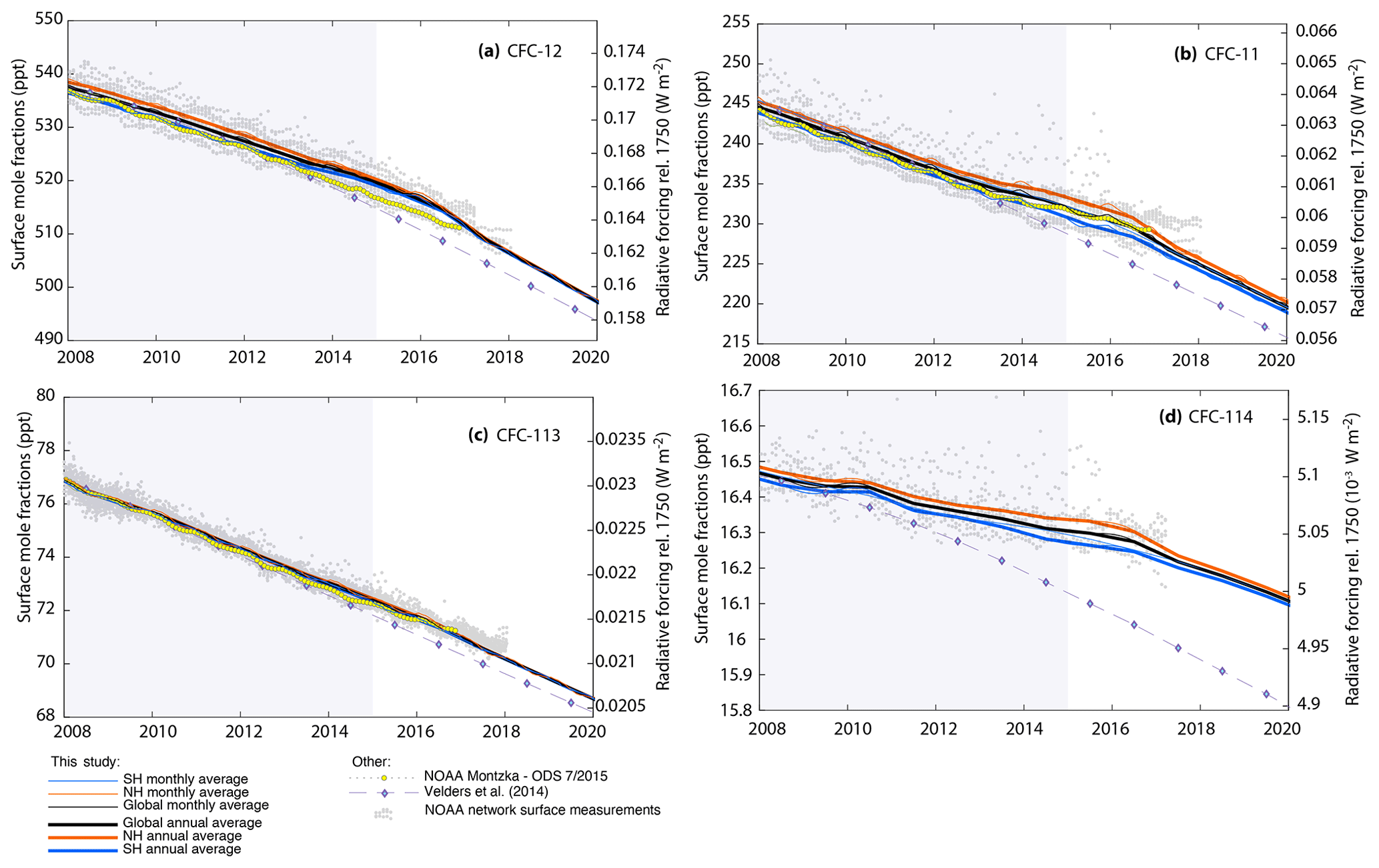
Figure 10 Atmospheric surface air mole fractions of four CFCs, namely CFC-12 (a), CFC-11 (b), CFC-113 (c), and CFC-114 (d). This study's northern hemispheric averages (orange lines), southern hemispheric averages (blue lines), and global averages (black lines) are shown in comparison with recent measurements of the NOAA and/or AGAGE networks (grey dots), the global averages derived by Montzka et al. (2018), and the projections by Velders and Daniel (2014) (dashed lines with diamond markers). The latter can be seen as near-lifetime limited projections, whereas observations hint at recent (since 2012) emissions increases, leading to a slower-than-projected fall in global atmospheric concentrations. For an exploration of CFC-11's decline rates, see the recent studies by Montzka et al. (2018) and Rigby et al. (2019). Note that the high “outlier” monthly mean values for CFC-11 and CFC-114 are primarily from the AGAGE Gosan station and include all data, i.e. so-called “pollution” events, in which case temporary high-concentration air masses pass the measurement station. The apparent disappearance of those high-pollution events at the end of 2015 is due to that particular AGAGE data time series only having been available until then at the point of this analysis, although a recent publication (Rigby et al., 2019) shows that these enhancements continued at least through 2017.

Chloroform (CHCl₃) exhibited a concentration decline since 2000 but is increasing again in the global atmosphere (see chloroform fact sheet available in the online data repository at http://greenhousegases.science.unimelb.edu.au). Fang et al. (2019) point to a recent strong growth of chloroform emissions in China. The similarly short-lived methylene chloride (CH₂Cl₂) also had almost stagnant atmospheric concentrations around the year 2000, but high growth has been observed in subsequent years, almost doubling atmospheric global-average concentrations from around 20 to 40 ppt by 2017 (Hossaini et al., 2015). See also chap. 1 of the 2018 Ozone Assessment Report (Engel et al., 2018).

Emissions of HFC-23 originate almost completely as a by-product of the production of HCFC-22. Under the Kyoto Protocol, abated emissions of HFC-23 are eligible to be credited in project-based offset mechanisms – leading to a bulk of offset credits under the Clean Development Mechanism and also two former joint implementation projects in Russia (Schneider, 2011). It has been shown that so-called “perverse incentives” likely resulted in additional production – in order to broaden the magnitude of claimable abatement credits (Schneider and Kollmuss, 2015). Given that the monetary value of those offset credits far exceeded the abatement costs, the Kigali Amendment to the Montreal Protocol in October 2016 led to a new regulatory approach for HFC emissions (Velders et al., 2015). Nevertheless, rather high individual station measurements (classified as “pollution” events) led to high monthly average concentrations at the Gosan South Korean station. Together with accelerating growth trends for HFC-23 since 2015, this could point to a continued large increase in emissions (see panel h in HFC-23-related fact sheets on http://greenhousegases.science.unimelb.edu.au). Similarly, SF₆ concentrations continue to increase at unprecedented rates. They will remain high for a long time (without other anthropogenic interventions) due to SF₆'s very long lifetime. The commonly assumed lifetime so far (also assumed in this study) has been 3200 years (Myhre et al., 2013), although recent findings about a loss mechanism in the polar vortex suggest a lower new best estimate of 850 years (Ray et al., 2017).

4.3 The long-term projections in the context of the last 2000 years

As the historical compilation of greenhouse gas concentrations based on firn and ice core records indicated, multiple literature studies indicate relatively flat concentrations of CO₂, CH₄, and N₂O over the past 2000 years. Historical fluctuations over the last 2000 years of a few parts per million or parts per billion, e.g. around 1650 for CO₂, are minuscule in comparison to recently observed concentration changes since the onset of industrialization and projected future changes (Fig. 8). For example, CO₂ concentrations could reach levels beyond 1500 ppm in the SSP3-7.0 and SSP5-8.5 scenarios and even reach beyond 2000 ppm by 2200 under SSP5-8.5. CO₂ concentrations in excess of 1500 ppm have likely not been present on Earth for more than 40 million years (Fig. 4 in Royer, 2006) – i.e. before the current Antarctic and Northern Hemisphere ice sheets formed. Reflecting the shorter lifetime, concentrations of methane decrease pronouncedly over the 21st century. The stronger mitigation scenarios foresee the option of net negative emissions for CO₂, so that CO₂ concentrations recede over the long term to around 350 ppm in the case of the SSP1-1.9 scenario. Reflecting the longer lifetime and base level of agricultural emissions, N₂O concentrations are not foreseen to drop below current levels in any of the investigated SSP scenarios over the coming 500 years (Fig. 8).

4.4 Comparing SSP and RCP concentrations

For every generation of climate scenarios, whether these are the IS92, SRES, RCP, or now the SSP scenarios, it is pertinent to clarify the differences and similarities of the new scenario set to the previous one(s). In particular due to the unavoidable delay in the analysis and use of the climate projections in the impact communities, clarifying the comparability to previous scenarios is paramount. Here, we compare the greenhouse gas concentrations.

Four RCP scenarios are now replaced in the SSP generation of scenarios with five high-priority scenarios (four ScenarioMIP “Tier1” cases plus SSP1-1.9) in addition to four additional scenarios that investigate additional forcing levels (see panels a, c in Fig. 11). Aside from this difference in the sheer number of scenarios, compared to the RCPs, the actual concentration levels differ substantially for most corresponding SSP scenarios. For example, the SSP5-8.5 scenario features substantially higher CO₂ concentrations by 2100 and beyond than the RCP8.5 scenario (panels a, b in Fig. 11). Somewhat compensating though, the CH₄ concentrations by 2100 are substantially lower under the SSP5-8.5 scenario compared to the RCP8.5 scenarios (Fig. 11c), and that difference is even more pronounced by 2300 due to the different extension principles followed for RCP extensions (Meinshausen et al., 2011b) and those for SSPs (Sect. 2.3). Specifically, the SSP5-8.5 fossil and industrial CH₄ emissions are assumed to be phased out by 2250 with land-use-related CH₄ emissions kept constant at 2100 under the SSP5-8.5 extension. That contrasts with the RCP8.5 extension, in which a long-term CH₄ concentration stabilization at very high levels of 3500 ppb was implemented. Similarly, for N₂O, the new SSP5-8.5 scenario implies lower concentrations by 2100 and beyond compared to the RCP8.5 (Fig. 11e, f). Under the SSP family, the SSP3-7.0 becomes the scenario with the highest emissions and concentrations for both CH₄ and N₂O.

Figure 11 Overview of SSP concentrations in comparison with RCP concentrations for CO₂, CH₄, and N₂O. The original RCP scenarios are shown in thicker black lines and various line styles. Applying the new MAGICC7 default setting used for the SSP scenarios to the RCP emissions results in generally higher concentrations (grey lines).

On the lower side of the scenarios, the most marked differences are that the new SSP1-2.6 has higher CO₂ concentrations, compared to the previous RCP2.6 and SSP1-1.9 has the lowest CO₂ concentrations (Figs. 9 and 11a). CH₄ concentrations are very similar across these three scenarios by the middle of the century, whereas by the end of the 21st century, the new SSP1-1.9 and SSP1-2.6 scenarios show reduced levels of only 1000 ppb, substantially below today's CH₄ concentration levels. For N₂O, the story is the other way around: SSP1-1.9 and SSP1-2.6 follow almost identical concentration trajectories, while the previous RCP2.6 scenario is lower.

4.5 Estimating the effect of latitudinally and seasonally resolved GHG concentrations on surface air temperatures in ESMs

A much-improved assimilation process results from considering seasonally and latitudinally resolved GHG concentration – as individual station monthly mean measurements can easily be “bias”-corrected to account for their latitudinal and seasonal variations to inform the global mean. In addition, however, the latitudinally and seasonally resolved GHG concentration data we provide also offer an opportunity to drive Earth system models with more accurate forcings, so that a comparison of the ESM historical runs with observational data can be performed – excluding ESM biases that might result from GHG concentrations that are applied with a globally uniform GHG concentration level or spatial fields that are sometimes rather dissimilar from observations (Figs. S46 and S47 in the Supplement of Meinshausen et al., 2017). In order to test the approximate magnitude of applying either globally uniform (“yearmean-global”) or latitudinally and seasonally resolved GHG concentrations (“lat-mon”), we performed six historical ensemble members of the CESM1.2.2 model (Hurrell et al., 2013) under each setup. To increase the signal-to-noise ratio, we then took the averages over the 155 years of model simulations from 1850 to 2005 across the six ensembles, resulting in 930 years of model data under each experiment. Given the seasonality of the data, we average the DJF (December–January–February) and MAM (March–April–May) monthly means in the “lat-mon” experiment and subtract the reference scenario's “yearmean-global” respective average. In the DJF and MAM northern hemispheric winter and spring season, one would expect a slight positive warming signal in the higher northern latitudes – given the latitudinal gradient of methane concentrations and the seasonally higher CO₂ concentrations. Indeed, we observe a regional warming signal of up to 0.4 K over northern American and Eurasian land masses, which is – in the DJF season – however latitudinally overcompensated by a strong cooling signal in the North Atlantic (Fig. 12a). In the MAM season, the slight cooling signal in the North Atlantic does not fully offset the warming over the land masses (Fig. 12b), resulting in a latitudinally averaged warming signal of approximately 0.1 K poleward of 65^∘ north (Fig. 12d). Given the high natural variability in the higher latitudes, we consider the significance of this warming signal by comparing our warming signal to corresponding differences of arbitrarily chosen control run segments. From an approximately 4500-year-long control run for CESM1.2.2 at pre-industrial conditions, we randomly chose 100 pairs of 930-year-long segments to compute the variability of the differences. It turns out that our warming signals are within the min–max range of those 100 sample pairs regarding the latitudinally averaged warming differences, indicating that the expected warming signal due to applying latitudinally and seasonally resolved GHG concentration data is not beyond the variability range. For the MAM period, there are only a few (approximately three to five) of the paired differences that result in a higher warming signal though, suggesting that the GHG warming signal might be comparable in magnitude to the variability to be expected at a 5 % confidence level. In the DJF period, a strong North Atlantic cooling is reducing the latitudinally aggregated warming signal. Whether that North Atlantic cooling is a result of natural variability in our modestly sized six-member ensembles or whether it is a dynamical response to generally higher-latitude forcing (and possible reduced overturning in the North Atlantic thermohaline circulation branch) cannot be detected from our initial ESM runs.

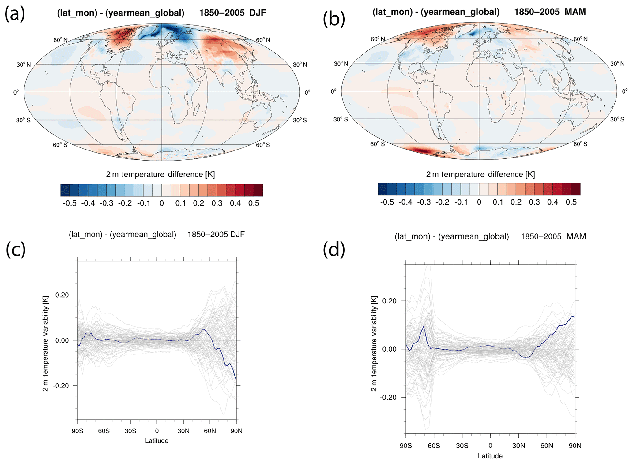
Figure 12 Warming signal induced by latitudinally and seasonally resolved GHG concentrations (“lat_mon”) compared to an annually and global-mean uniform GHG concentrations (“yearmean_global”) in an Earth system model, namely CESM1.2.2 (Hurrell et al., 2013). We averaged the full historical scenario from 1850 to 2005 across all six ensemble members in each setup (“lat_mon” and “yearmean_global”) and produced the averages for the December–January–February DJF average (a) and the March–April–May averages (b). The latitudinally averaged warming signals that result from using spatially and temporarily resolved GHG concentrations are shown in (c) and (d) (thick blue lines), here compared against comparable 100 differenced pairs of 930-year-long control run segments (thin grey lines). In the high upper north during the MAM season, the comparison with control run segment differences suggests that these ESM model results show a significant warming at the 5 % level, given that only 3 to 5 of the 100 control run differences are higher.

As one would expect, our analysis does not suggest significant latitudinal temperature perturbations at the 5 % level for the JJA (June–July–August) and SON (September–October–November) periods (not shown), when seasonally lower CO₂ concentrations are partially offset by the latitudinal gradient of concentrations in the Northern Hemisphere

5 Limitations

In this section, we provide a number of key limitations that come with the SSP concentration datasets. Some of these limitations arise from the underlying emission scenario data (Sect. 5.1 and 5.2), some due to imperfect matches between recent observational and model results (Sect. 5.3), some are intrinsic model limitations (Sect. 5.4 and 5.5). Likely the largest limitation is that – by design – this study provides default concentration time series for the future but does not represent the uncertainty range of future greenhouse gas concentrations for each scenario (Sect. 5.6).

5.1 Limited emission variations across scenarios for gases other than CO₂, CH₄, and N₂O

The main focus of integrated assessment models rests on projecting sectorally resolved energy, transport, industry, waste, agricultural, and land use emissions for CO₂, CH₄, and N₂O as well as air pollutant emissions. The other industrial greenhouse gases in the basket of gases of the Kyoto Protocol, namely HFCs, PFCs, SF₆, and NF₃, are often modelled as a group or in subgroups. Subsequent downscaling mechanisms can then yield individual gas time series, although they often lack specific process dynamics, i.e. following the same growth and decline trajectory independent of their actual end-use applications. This is certainly a limitation of many of the forward-looking PFC projections.

In terms of the ozone-depleting substances (ODSs), a feature, or limitation, is that the presented SSP scenarios do not capture baseline or reference scenarios or in fact any emission-driven scenario variation at all. This is because the future ODS emissions are strongly constrained by the Montreal Protocol phase-out schedules. The real-world uncertainty in ODS emissions comes from non-compliance to the Protocol and from uncertainties in emission factors from banks and bank magnitudes. In our study, in which we assume identical emissions in all of our different scenarios, future variations in concentrations are hence purely climate-driven, i.e. illustrate the effect that circulation or atmospheric chemistry changes across the scenarios can have on the ODS lifetimes. It might be worth considering whether, for future assessments, the climate community's scenarios and the ozone community's scenarios could not be commonly designed. For example, some of the scenarios could include ODS emission futures that reflect lower or even non-compliance with the Montreal Protocol to allow studies on the “world avoided” (Morgenstern et al., 2008; Velders et al., 2007). An integration of scenarios used for the ozone assessments and the climate assessments may be desirable.

Finally, another limitations is that a few minor long-lived greenhouse gases are not included in this compilation of 43 gases, such as CFC-13 or the isomer CFC-114a (Vollmer et al., 2018).

5.2 Individual scenario features and overall scenario spectrum

Despite all the multi-year design efforts by large research international communities, there are some inevitable limitations of the overall group of scenarios. In particular, the final set of scenarios might be more appropriate for the Earth system research community than for those interested in exploring policy-relevant outcomes. For example, one of the scenarios that features new characteristic is the SSP5-3.4-OS scenario. That scenario assumes the greatest net negative emissions after an initial high-emission growth rate. Its high-peak-then-strong-decline feature tests the biophysical models and will be pivotal to examining the asymmetry of the ramp-up and ramp-down characteristics of the carbon cycle, ocean heat uptake, and multiple other Earth system properties. Yet, for policy purposes, that is substantially outside the target space of the Paris Agreement, aiming to keep temperatures to below 2 ^∘C warming.

A possible shortcoming for the climate science and impact community is that the new SSP generation of scenarios does not provide a very closely matching overlap with the RCP scenarios, as multiple scenario features are substantially different (see, e.g., CO₂ and CH₄ concentrations in Fig. 9). Thus, from a climate science perspective, maintaining a single multi-gas scenario unaltered from the previous generation of scenarios could have provided a useful reference point with which to quantify the change in our climate system knowledge for future projections. Given the amount of human and material resources used for the CMIP6 runs, it is, however, a question of balance between historical comparability and the capability to link to earlier studies and putting resources into the most relevant, up-to-date, scenarios. However, there is also a desire to use the best available forcing data to simulate the historical period. Because the actual historical evolution of concentrations and SLCF emissions has been different in detail from previous scenarios and historical emission and concentration estimates are updated over time (e.g. Hoesly et al., 2018), the community has thus far decided to use the most up to date data for each subsequent CMIP exercise.

5.3 Transition issues from observational to modelled concentrations

MAGICC has been calibrated to allow a smooth continuation from historical time series to future projections. For some gases, this transition is possibly suboptimal. For example, atmospheric measurements since 2013 produced some rather high chloroform (CHCl₃) concentrations in the Northern Hemisphere, which lead to a stronger latitudinal gradient assumption in the assimilation framework for those recent years. The future projections do not reflect a continuation of this high implied emission spike and hence revert to a lower latitudinal gradient and slightly smaller global-mean chloroform concentrations (see panel f in the Chloroform fact sheet available on http://greenhousegases.science.unimelb.edu.au). A similar transition issue is also present for HFC-23, HFC-245fa, HFC-43-10mee, CH₂Cl₂, and Halon-1301 and even more pronounced for HFC-32, whose actual global emissions seem to increase much more strongly than assumed in the 2020s in our Kigali-aligned emission scenario by Velders et al. (2015).

5.4 Main limitations due to sequential scenario generation process

The sequential and concentration-driven nature of the main ESM CMIP6 experiments poses the challenge that future projections of greenhouse gas concentrations are required before the ESM results can be evaluated. In other words, the best estimate of future CO₂ concentrations, given a certain emission pathway, will certainly differ at the end of the CMIP6 analysis cycle from the setting with which the MAGICC7 climate model was driven for this study. This sequential problem could only be avoided with an altered experimental design, performing most future ESM experiments in an emission-driven, but computationally more demanding, design. An advantage of the concentration-driven runs is that climate feedbacks and carbon cycle feedbacks can more easily be separated.

In addition to the inconsistencies introduced by the sequential and concentration-driven nature of future climate scenario experiments, there are clearly limitations of MAGICC and its chosen default parameter settings for this study. A full evaluation of the extent to which the chosen parameters yield a concentration response that is representative of the higher-complexity atmospheric chemistry model projections that are part of CMIP6 will be of key interest for future studies.

5.5 Variable natural emissions

Except for the interactive carbon cycle, this study assumes constant natural emissions levels for substances like CH₄, N₂O, CH₃Br, CH₃Cl, and others. This is clearly a limitation, as under climate change and human management of the land and ocean, the magnitude of these natural emissions (indirectly influenced by human activities) will change over time. Future research could build knowledge of the time-varying natural emission sources into the projection model used.

5.6 No uncertainty estimates

A major limitation of our study is the lack of uncertainty estimates. Given the primary purpose of this study of providing a single reference concentration projection as input dataset for the CMIP6 experiments, uncertainty ranges around the projections are not necessary. However, in multiple other potential applications of this dataset, properly derived uncertainty information could have opened up new use cases. For example, simple inversion studies could attempt to derive seasonally varying sink and source patterns from our observationally based historical monthly and latitudinally resolved concentration patterns. Without the appropriate uncertainty information, any inversion approach will have to make ad hoc assumptions.

6 Conclusions

The projected human-induced increase in atmospheric greenhouse gas abundances over the 21st century swamps all observed variations for the last 2000 years (Fig. 8). The new SSP scenarios span an even broader range of CO₂ concentration futures, with the higher end (SSP5-8.5) yielding higher concentrations than the previous RCP8.5 scenario and the lower end SSP1-1.9 scenario resulting in CO₂ emissions down to 350 ppm in the longer term (2150). Also, in a more technical aspect, the SSP concentrations are breaking new ground. For the first time, the greenhouse gas projections are available for 43 greenhouse gases, with latitudinal and seasonal variations captured. For example, by 2050, northern hemispheric concentrations in the SSP3-7.0 scenario are 1.2 % and 4.3 % higher than southern hemispheric averages for CO₂ and CH₄, respectively – with corresponding non-negligible implications for radiative forcing (Table 5).

Given the substantial efforts that go into the data collection by observational network communities, a worthwhile effort in continuation from the present study would be to build a real-time framework to provide a system that updates GHG historical and future projections, including uncertainties, for a wide range of – perhaps also updated – scenarios from the integrated assessment community. While updates of observations, gas cycle models, or emission scenarios in between the major IPCC or WMO assessments are useful for a range of scientific studies, the new GHG projections data could be frozen every several years to provide a new range of benchmark scenarios for Earth system models. Efforts to provide more frequent updates for emissions data are also underway (e.g. Hoesly et al., 2018).

More than 20 years ago, the IPCC started to put forward future concentration scenarios, the so-called IS-92 scenarios. Back then in 1992, CO₂ concentrations were at 356 ppm (Keeling et al., 1976; Keeling and Whorf, 2004). In 2019, atmospheric CO₂ concentrations are 411 ppm. In equilibrium and assuming a central climate sensitivity of 3 ^∘C, these CO₂ concentrations of 411 ppm alone would imply a temperature change of 1.7 ^∘C above pre-industrial levels (using the simple and standard CO₂ forcing formula of RF $=\mathrm{5.35}\times \ln (C/C_{\mathrm{0}})$ with C being the current and C₀ being the pre-industrial concentrations). While zero CO₂ emissions would yield decreasing concentrations, it becomes clear that only a future emission trajectory that effectively reduces atmospheric CO₂ concentration levels below today's levels would provide a reasonable chance to keep warming at or below 1.5 ^∘C in the longer term. And even such 1.5 ^∘C of warming could come with multi-metre sea level rise by 2300 (Mengel et al., 2018) and the likely demise of coral reefs (Frieler et al., 2013). Thus, while the scenarios shown span a scientifically valid wide range of plausible futures, from a climate impact point of view – and trying to achieve the Paris Agreement targets – all except for the lowest scenarios investigated in this study will hopefully remain hypothetical futures.