the Creative Commons Attribution 4.0 License.
the Creative Commons Attribution 4.0 License.
PDE-NetGen 1.0: from symbolic partial differential equation (PDE) representations of physical processes to trainable neural network representations
Olivier Pannekoucke
Ronan Fablet
Bridging physics and deep learning is a topical challenge. While deep learning frameworks open avenues in physical science, the design of physically consistent deep neural network architectures is an open issue. In the spirit of physics-informed neural networks (NNs), the PDE-NetGen package provides new means to automatically translate physical equations, given as partial differential equations (PDEs), into neural network architectures. PDE-NetGen combines symbolic calculus and a neural network generator. The latter exploits NN-based implementations of PDE solvers using Keras. With some knowledge of a problem, PDE-NetGen is a plug-and-play tool to generate physics-informed NN architectures. They provide computationally efficient yet compact representations to address a variety of issues, including, among others, adjoint derivation, model calibration, forecasting and data assimilation as well as uncertainty quantification. As an illustration, the workflow is first presented for the 2D diffusion equation, then applied to the data-driven and physics-informed identification of uncertainty dynamics for the Burgers equation.
- Article
(1455 KB) - Full-text XML
- BibTeX
- EndNote
Machine learning and deep learning are of fast-growing interest in geoscience to address open issues, including sub-grid parameterization.
A variety of learning architectures have shown their ability to encode the physics of a problem, especially deep learning schemes which typically involve millions of unknown parameters, while the theoretical reason for this success remains a key issue (Mallat, 2016). A recent research trend has involved the design of lighter neural network (NN) architectures, like residual neural networks (ResNets) with shared weights (He et al., 2016), while keeping a similar learning performance. Interestingly, a ResNet can be understood as an implementation of a numerical time scheme solving an ordinary differential equation (ODE) or partial differential equation (PDE) (Ruthotto and Haber, 2019; Rousseau et al., 2019). Applications to learning PDEs from data have also been introduced, e.g. PDE-Net (Long et al., 2017, 2018). These previous works emphasize the connection between the underlying physics and the NN architectures.
Designing or learning an NN representation for a given physical process remains a difficult issue. If the learning fails, it may be unclear how to improve the architecture of the neural network. It also seems irrelevant to run computationally expensive numerical experiments on a large-scale dataset to learn well-represented processes. The advection in fluid dynamics may be a typical example of such processes, which do not require complex non-linear data-driven representations. Overall, one would expect to accelerate and make more robust the learning process by combining, within the same NN architecture, the known physical equations with the unknown physics.
From the geoscience point of view, a key question is to bridge physical representations and neural network ones so that we can decompose both known and unknown equations according to the elementary computational units made available by state-of-the-art frameworks (e.g. Keras, TensorFlow). In other words, we aim to translate physical equations into the computational vocabulary available to neural networks. PDE-NetGen (Pannekoucke, 2020) addresses this issue for PDE representations, for which we regard convolutional layers as being similar to the stencil approach, which results from the discretization of PDEs by using the finite-difference method (see e.g. Thomas, 1995). PDE-NetGen relies on two main components: (i) a computer algebra system, here SymPy (Meurer et al., 2017), used to handle the physical equations and discretize the associated spatial derivatives; and (ii) a Keras network generator which automatically translate PDEs into neural network layers from these discretized forms. Note that code generators based on symbolic computation are receiving increased attention to facilitate the design of numerical experiments; see e.g. Louboutin et al. (2019). As an illustration, we consider in this paper the application of PDE-NetGen to the identification of closure terms.
The paper is organized as follows. In the next section, we detail the proposed neural network generator, with an illustration of the workflow on a diffusion equation. In Sect. 3, we present the numerical integration of the neural network implementation of the diffusion equation, then an application to the data-driven identification of the closure of the Burgers equation. A conclusion and perspective are given in Sect. 4
Introducing physics in the design of neural network topology is challenging since physical processes can rely on very different partial derivative equations, e.g. eigenvalue problems for waves or constrained evolution equations in fluid dynamics under iso-volumetric assumption. The neural network code generator presented here focuses on physical processes given as evolution equations:
where u denotes either a scalar field or multivariate fields, ∂αu denotes partial derivatives with respect to spatial coordinates, and ℳ is the generator of the dynamics. At first glance, this situation excludes diagnostic equations as encountered in geophysics, like balance equations: each equation has to be the evolution equation of a prognostic variable. PDE-NetGen incorporates a way to solve diagnostic equations, and this will be shown in the example detailed in Sect. 3.2.
We first explain how the derivatives are embedded into NN layers, then we detail the workflow of PDE-NetGen for a simple example.
2.1 Introducing physical knowledge in the design of an NN topology
Since the NN generator is designed for evolution equations, the core of the generator is the automatic translation of partial derivatives with respect to spatial coordinates into layers. The correspondence between the finite-difference discretization and the convolutional layer give a practical way to translate a PDE into an NN (Cai et al., 2012; Dong et al., 2017; Long et al., 2017).
The finite-difference method remains to replace the derivative of a function by a fraction that only depends on the value of the function (see e.g. Thomas, 1995). For instance, the finite-difference method applied on a second-order partial derivative , for u(t,x) on a 1D domain, leads to the approximation of the derivative by
with
where δx stands for the discretization space step. Here the spatial derivative is replaced by a fraction that only depends on the values of u at the time t and points x−δx, x, x+δx. This makes a kernel stencil appear that can be used in a 1D convolution layer with a linear activation function and without bias. A similar routine applies for 2D and 3D geometries. PDE-NetGen relies on the computer algebra system SymPy (Meurer et al., 2017) to compute the stencil and to handle symbolic expressions.
In PDE-NetGen, the finite-difference implementation appears as a linear operator ℱ which approximates any partial derivative from the values on a regular grid. In particular, the finite difference of any partial derivative of order α, is computed from the grid points when is odd and when α=2p is even. This approximation is consistent at the second order, i.e. , where 𝒪 is Landau's big O notation: for any f, the notation means that is finite.
The operator ℱ behaves partially as the partial derivative operator ∂: ℱ is commutative with respect to independent coordinates, i.e. in a 2D domain for coordinates (x,y) we have , where ∘ denotes the operator composition, and this applies at any order, e.g. (but ). Hence, the finite difference of a derivative with respect to multiple coordinates is computed sequentially from the iterative discretization along each coordinate, and this approximation is consistent at the second order.
Note that we chose to design PDE-NetGen considering the finite-difference method, but alternatives using automatic differentiation can be considered as introduced by Raissi (2018), who used TensorFlow for the computation of the derivative.
Then, the time integration can be implemented either by a solver or by a ResNet architecture of a given time scheme, e.g. an Euler scheme or a fourth-order Runge–Kutta (RK4) scheme (Fablet et al., 2017).
These two components, namely the translation of partial derivatives into NN layers and a ResNet implementation of the time integration, are the building blocks of the proposed NN topology generator as exemplified in the next section.
2.2 Workflow of the NN representation generator
We now present the workflow for the NN generator given a symbolic PDE using the heterogeneous 2D diffusion equation as a test bed:
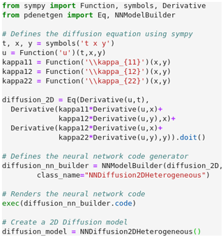
where is a field of 2×2 diffusion tensors, with x and y as the spatial coordinates, and whose Python implementation is detailed in Fig. 1.
Starting from a list of coupled evolution equations given as a PDE, a first preprocessing of the system determines the prognostic functions, the constant functions, the exogenous functions and the constants. The exogenous functions are the functions which depend on time and space but whose evolution is not described by the system of evolution equations. For instance, a forcing term in dynamics is an exogenous function.
For the diffusion equation Eq. (4),
the dynamics are represented in SymPy using the Function,
Symbol and Derivative classes.
The dynamics are defined as an equation using the Eq class of PDE-NetGen,
which inherits from sympy.Eq
with additional facilities (see the implementation in Fig. 1 for additional details).
The core of the NN generator is given by the NNModelBuilder class. This class first preprocesses the system of evolution equations and translates the system into a Python NN model.
The preprocessing of the diffusion equation Eq. (4)
presents a single prognostic function, u, and three
constant functions κ11, κ12 and κ22. There is no exogenous function for this example. During the preprocessing, the coordinate system of each function is diagnosed such that we may determine
the dimension of the problem. For the diffusion equation (Eq. 4), since the function is a function of (x,y) the geometry is two-dimensional.
In the current version of PDE-NetGen, only periodic boundaries are considered. The specific DerivativeFactory class ensures
the periodic extension of the domain, then the computation of the derivative by using a convolutional neural network (CNN) and finally the crop of the extended domain to return to the initial domain. Other boundaries could also be implemented and might be investigated in future developments.
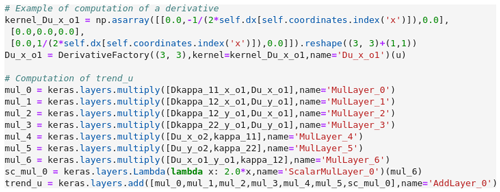
Figure 2 Part of the Python code of the
NNDiffusion2DHeterogeneous class,
which implements the diffusion equation (Eq. 4) as a neural network by using Keras (only
one derivative is explicitly given for the sake of simplicity).
All partial derivatives with respect to spatial coordinates are detected and then replaced by an intermediate variable in the system of evolution equations. The resulting system is assumed to be algebraic, which means that it only contains addition, subtraction, multiplication and exponentiation (with at most a real). For each evolution equation, the abstract syntax tree is translated into a sequence of layers which can be automatically converted into NN layers in a given NN framework. For the current version of PDE-NetGen, we consider Keras (Chollet, 2018). An example of the implementation in Keras is shown in Fig. 2: a first part of the code is used to compute all the derivatives using Conv layers of Keras, then Keras layers are used to implement the algebraic equation, which represents the trend ∂tu of the diffusion equation Eq. (4).
At the end, a Python code is rendered from templates by using the jinja2 package. The reason why templates are used is to facilitate the saving of the code in Python modules and the modification of the code by the experimenter. Runtime computation of the class could be
considered, but this is not implemented in the current version of PDE-NetGen. For the diffusion equation (Eq. 4), when run, the code rendered from the NNModelBuilder class
creates the NNDiffusion2DHeterognous class. Following the class diagram in Fig. 3, the NNDiffusion2DHeterogeneous class inherits from a Model class, which
implements the time evolution of evolution dynamics by incorporating a time scheme. Here several time schemes are implemented, namely an explicit Euler scheme and a second- and a fourth-order Runge–Kutta scheme.
Two applications are now considered. First we validate the NN generator on a known physical problem: the diffusion equation (Eq. 4) detailed in the previous section. Then, we tackle a situation in which part of the physics remains unknown, showing the benefit of merging the known physics in the learning of the unknown processes.
3.1 Application to the diffusion equation
In the Python implementation in Fig. 1,
diffusion_model is an instance of the NNDiffusion2DHeterogeneous class,
which numerically solves the diffusion equation (Eq. 4) over a 2D domain, defined by default as the periodic domain discretized by 100 points along each direction so that .
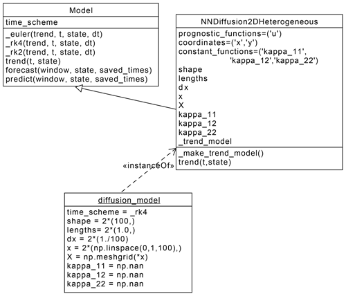
Figure 3Unified modelling language (UML) class diagram showing the interaction between the Model and the NNDiffusion2DHeterogeneous classes,
as well as the resulting instance diffusion_model
corresponding to the numerical computation of the diffusion equation (Eq. 4).
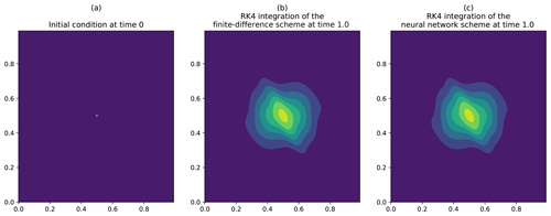
The time integration of the diffusion equation is shown in Fig. 4. For this numerical experiment, the heterogeneous tensor field of diffusion tensors κ(x,y) is set as rotations of the diagonal tensor defined from the length scales lx=10 dx and ly=5 dy and the timescale τ=1.0, with the rotation angles , where . The time step for the simulation is . The numerical integration is computed by using a fourth-order Runge–Kutta scheme. The initial condition of the simulation is given by a Dirac in Fig. 4a. In order to validate the solution obtained from the generated neural network, we compare the integration with the one of the finite-difference discretization of Eq. (4),
where ℱ is the operator described in Sect. 2.1 and whose numerical result is shown in Fig. 4b.
The heterogeneity of the diffusion tensors makes an anisotropic diffusion of the Dirac appear (see Fig. 4b), which is perfectly reproduced by the result obtained from the integration of the generated neural network, as shown in Fig. 4c. At a quantitative level, the l2 distance between the solutions is 10−5 (with ). This validates the ability of the NN generator PDE-NetGen to compute the dynamics of a given physical evolution equation.
The next section illustrates the situation in which only part of the dynamics is known, while the remaining physics are learned from the data.
3.2 Application to the data-driven identification of stochastic representations
As an illustration of the PDE-NetGen package, we consider a problem encountered in uncertainty prediction: the parametric Kalman filter (PKF) (Pannekoucke et al., 2016, 2018). For a detailed presentation and discussion of uncertainty prediction issues in geophysical dynamics, we refer the reader to Le Maître and Knio (2010). Here, we briefly introduce basic elements for the self-consistency of the example.
The idea of the PKF is to mimic the dynamics of the covariance error matrices all along the analysis and the forecast cycle of the data assimilation in a Kalman setting (Kalman filter equations for the uncertainty). It relies on the approximation of the true covariance matrices by some parametric covariance model. When considering a covariance model based on a diffusion equation, the parameters are the variance V and the local diffusion tensor ν. Therefore, the dynamics of the covariance error matrices along the data assimilation cycles are deduced from the dynamics of the variance and of the diffusion tensors. In place of the full covariance evolution this dramatically reduces the dynamics to one of few parameters.
For the non-linear advection–diffusion equation, known as the Burgers equation,
the dynamics of the variance Vu and the diffusion tensor (which is featured by a single field νu,xx) (Pannekoucke et al., 2018) are the following.
Here, 𝔼[⋅] denotes the expectation operator. For the sake of simplicity, in this system of PDEs, u denotes the expectation of the random field and not the random field itself as in Eq. (6).
In this system of PDEs, the term cannot be determined from the known quantities u,Vu and νu,xx. This brings up a problem of closure, i.e. determining the unknown term as a function of the known quantities. A naive assumption would be to consider a zero closure (. However, while the tangent–linear evolution of the perturbations along the Burgers dynamics is stable, the dynamics of the diffusion coefficient νu,xx would lead to unstable dynamics as the coefficient of the second-order term is negative. This further stresses the importance of the unknown term to successfully predict the uncertainty.
Within a data-driven framework, one would typically explore a direct identification of the dynamics of the diffusion coefficient νu,xx. Here, we use PDE-NetGen to fully exploit the known physics and focus on the data-driven identification of the unknown term in the system of equations (Eq. 7). This leads to replacing the term in Eq. (7) by an exogenous function closure(t,x) and then to follow the workflow detailed in Sect. 2.2.
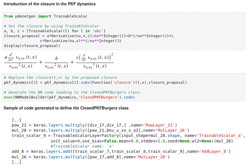
Figure 5
Implementation of the closure by defining each unknown quantity as an instance of the class TrainableScalar
and the resulting generated NN code.
This is part of the code available in the Jupyter notebook given as an example in the package PDE-NetGen.
The unknown closure function is represented by a neural network (a Keras model) which implements the expansion
where a, b, and c are unknown and where the partial derivatives are computed from convolution layers, as described in Sect. 2. This expression is similar to a dictionary of possible terms as in Rudy et al. (2017), and it is inspired from an arbitrary theoretically designed closure for this problem where (see Appendix A for details). In the NN implementation of the exogenous function modelled as Eq. (8), each of the unknown coefficients is implemented as a 1D convolutional layer, with a linear activation function and without bias. Note that the estimated parameters could be different from the one of the theoretical closure: while the theoretical closure can give some clues for the design of the unknown term, this closure is not the truth, which is unknown (see Appendix A).
The above approach, which consists of constructing an exogenous function given by an NN to be determined, may seem tedious for an experimenter who would not be accustomed to NNs. Fortunately, we have considered an alternative in PDE-NetGen that can
be used in the particular case in which candidates for a closure take the form of an expression with
partial derivatives, as is the case for Eq. (8).
An example of implementation is shown in Fig. 5 where pkf_dynamics stands for the system of equations (Eq. 7). The unknown closure function is replaced by
the proposal of closure Eq. (8)
where each unknown quantity is declared as an instance of the class TrainableScalar.
Then, the NN is generated, producing the class ClosedPKFBurgers whose an instance is
ready for training. In the generated code, each instance of the TrainableScalar class is translated as
a specific layer, TrainableScalarLayerFactory,
equivalent to the above-mentioned convolution layer and whose parameter can be trainable. For instance, the trainable scalar a is implemented by the line train_scalar_9. Note that the layer TrainableScalarLayerFactory can be used for 1D, 2D or 3D domains.
In this example, the proposal for closure has been defined at a symbolic level without an additional
exogenous NN.
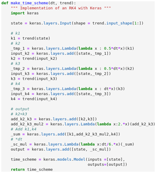
Figure 6
Example of a Keras implementation for an RK4 time scheme: given time step dt and a Keras model trend
of the dynamics, the function make_time_scheme
returns a Keras model implementing an RK4.
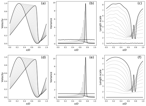
Figure 7 Uncertainty estimated from a large ensemble of 1000 members (a–c) with the expectation of 𝔼[u] (a), variance Vu (b) and the length scale (defined from the diffusion coefficient by ). (c) The uncertainty predicted from the PKF evolution equations closed from the data (d–f), for which the same statistics are shown in (d), (e) and (f). The fields are represented only for time .
Examples of implementation for the exogenous NN and for the trainable layers are provided in the package PDE-NetGen as Jupyter notebooks for the case of the Burgers equation.
For the numerical experiment, the Burgers equation is solved on a one-dimensional periodic domain of length 1, discretized in 241 points. The time step is dt=0.002, and the dynamics are computed over 500 time steps to integrate from t=0 to t=1.0. The coefficient of the physical diffusion is set to κ=0.0025. The numerical setting considered for the learning is the tangent–linear regime described in Pannekoucke et al. (2018), in which the initial uncertainty is small and whose results are shown in their Figs. 4a, 5a and 6a.
To train the parameters in Eq. (8), we build a training dataset from an ensemble prediction method whereby each member is a numerical solution of the Burgers equation. The numerical code for the Burgers equation derives from PDE-NetGen applied on the symbolic dynamics (Eq. 6). Using this numerical code, we generate a training dataset composed of 400 ensemble simulations of 501 time steps, with each ensemble containing 400 members. For each ensemble forecast, we estimate the mean, variance Vu and diffusion tensor νu. Here, we focus on the development of the front where we expect the unknown term to be of key importance and keep for training purposes the last 100 time steps of each ensemble forecast. For the training only, the RK4 time scheme is computed as the ResNet implementation given in Fig. 6 to provide the end-to-end NN implementation of the dynamics.
The resulting dataset involves 40 000 samples. To train the learnable parameters , we minimize the one-step-ahead prediction loss for the diffusion tensor νu. We use the ADAM optimizer (Kingma and Ba, 2014) and a batch size of 32. Using an initial learning rate of 0.1, the training converges within three outer loops of 30 epochs with a geometrical decay of the learning rate by a factor of 1∕10 after each outer loop. The coefficients resulting from the training over 10 runs are .
Figure 7 compares the estimation from a large ensemble of 1000 members (panels a–c) with the results of the trained closed PKF dynamics (panels d–f). Both the ensemble and PKF means (panels a and d) clearly show a front which emerges from the smooth initial condition located near x=0.75 at time 1. The variance fields (panels b and e) illustrate the vanishing of the variance due to the physical diffusion (the κ term in Eq. 6) and the emergence of a peak of uncertainty which is related to the uncertainty of the front position. Instead of the diffusion νu,xx, panels (c) and (f) show the evolution of the correlation length scale defined as , which has the physical dimension of a length. Both panels show the increase in the length scale due to the physical diffusion, except in the vicinity of the front where an oscillation occurs, which is related to the inflexion point of the front. While the magnitude of the oscillation predicted by the PKF (panel f) is slightly larger than the estimation from the large ensemble reference (panel c), the pattern is well-predicted by the PKF. In addition, the parametric form of the PKF does not involve local variabilities due to the finite size of the ensemble, which may be observed in panel (c). Overall, these experiments support the relevance of the closure in Eq. (8) learned from the data to capture the uncertainty associated with Burgers' dynamics.
3.3 Discussion on the choice of a closure
In the Burgers dynamics, a priori knowledge was introduced to propose an NN implementing the closure in Eq. (8).
In the general case, the choice of the terms to be introduced in the closure may be guided by known physical properties that need to be verified by the system. For example, conservation or symmetry properties that leave the system invariant can guide the choice of possible terms. For Burgers dynamics, νu,xx has the dimension of a length squared, [L2], and is of dimension [L−4]. Thus, the terms considered in Eq. (8) are among the simplest ones which fulfil the expected dimensionality of [L−4]. Symbolic computation here may help the design of such physical parameterizations in more general cases.
When no priors are available, one may consider modelling the closure using state-of-the-art deep neural network architectures, which have shown impressive prediction performance, e.g. CNNs, ResNets (Zagoruyko and Komodakis, 2016; Raissi, 2018).
The aim of the illustration proposed for Burgers dynamics is not to introduce a deep learning architecture
for the closure, but to facilitate the construction of a deep learning architecture taking into account the known physics: the
focus is on the hybridization between physics and machine learning. Though the closure
itself may not result in a deep architecture, the overall generated model leads to a deep
architecture. For instance, the implementation using the exogenous NN uses around 75 layers, while the
implementation based on the class TrainableScalar uses 73 layers
(we save the calculation of the derivatives that appear in Eq. (8), while they
are computed twice when using the exogenous NN),
with several convolutional layers among them.
For other problems, there would be no
choice other than considering a deep neural network, for instance using multiple ResNet blocks or
normalization, or architectures inspired from recent studies on closure modelling (e.g.
Bolton and Zanna, 2019). Such architectures can be plugged in PDE-NetGen as an exogenous neural network.
We have introduced a neural network generator, PDE-NetGen, which provides new means to bridge physical priors given as symbolic PDEs and learning-based NN frameworks. This package derives and implements a finite-difference version of a system of evolution equations, wherein the derivative operators are replaced by appropriate convolutional layers including the boundary conditions. The package has been developed in Python using the symbolic mathematics libraries SymPy and Keras.
We have illustrated the usefulness of PDE-NetGen through two applications: a neural network implementation of a 2D heterogeneous diffusion equation and the uncertainty prediction in the Burgers equation. The latter involves unknown closure terms, which are learned from data using the proposed neural network framework. Both illustrations show the potential of such an approach, which could be useful for improving the training in complex applications by taking into account the physics of the problem.
This work opens new avenues to make the most of existing physical knowledge and of recent advances in data-driven settings, more particularly neural networks, for geophysical applications. This includes a wide range of applications, for which such physically consistent neural network frameworks could either lead to the reduction of computational cost (e.g. GPU implementation embedded in deep learning frameworks) or provide new numerical tools to derive key operators (e.g. adjoint operator using automatic differentiation). These neural network representations also offer new means to complement known physics with the data-driven calibration of unknown terms. This is regarded as key to advancing state-of-the-art simulations, forecasting and the reconstruction of geophysical dynamics through model–data coupled frameworks.
For self-consistency, we detail how the theoretical closure is obtained (Pannekoucke et al., 2018).
It can be shown that , where is the so-called metric tensor that is a scalar field in 1D. When the correlation function is a homogeneous Gaussian, , where the metric tensor g is a constant here, then the fourth-order Taylor expansion in δx of the Gaussian correlation leads to the identity , which is independent of the position x. As a possible closure, this suggests modelling the unknown term as that depends on x. Replacing gu by 1∕(2νu) leads to
The result is that Eq. (A1) is not the true analytic expression of as a function of u,Vu and νu but only a parameterization.
The PDE-NetGen package is free and open source. It is distributed under the CeCILL-B free software licence. The source code is provided through a GitHub repository at https://github.com/opannekoucke/pdenetgen, last access: 12 June 2020). A snapshot of PDE-NetGen 1.0 is available at https://doi.org/10.5281/zenodo.3891101 (Pannekoucke, 2020).
OP and RF designed the study, conducted the analysis and wrote the paper. OP developed the code.
The authors declare that they have no conflict of interest.
The UML class diagram has been generated from UMLlet (Auer et al., 2003).
This work was supported by the French national programme LEFE/INSU (Étude du filtre de KAlman PAramétrique, KAPA). RF has been partially supported by Labex Cominlabs (grant SEACS), CNES (grant OSTST-MANATEE) and ANR through the programmes EUR Isblue, Melody and OceaniX.
This paper was edited by Adrian Sandu and reviewed by two anonymous referees.
Auer, M., Tschurtschenthaler, T., and Biffl, S.: A Flyweight UML Modelling Tool for Software Development in Heterogeneous Environments, in: Proceedings of the 29th Conference on EUROMICRO, EUROMICRO '03, 267 pp., IEEE Computer Society, Washington, DC, USA, https://doi.org/10.5555/942796.943259, 2003. a
Bolton, T. and Zanna, L.: Applications of Deep Learning to Ocean Data Inference and Subgrid Parameterization, J. Adv. Model. Earth Syst., 11, 376–399, https://doi.org/10.1029/2018ms001472, 2019. a
Cai, J.-F., Dong, B., Osher, S., and Shen, Z.: Image restoration: Total variation, wavelet frames, and beyond, J. Am. Math. Soc., 25, 1033–1089, https://doi.org/10.1090/s0894-0347-2012-00740-1, 2012. a
Chollet, F.: Deep Learning with Python, Manning Publications, 2018. a
Dong, B., Jiang, Q., and Shen, Z.: Image Restoration: Wavelet Frame Shrinkage, Nonlinear Evolution PDEs, and Beyond, Multiscale Model. Sim., 15, 606–660, https://doi.org/10.1137/15m1037457, 2017. a
Fablet, R., Ouala, S., and Herzet, C.: Bilinear residual Neural Network for the identification and forecasting of dynamical systems, ArXiv, arXiv:1712.07003, 2017. a
He, K., Zhang, X., Ren, S., and Sun, J.: Deep Residual Learning for Image Recognition, in: 2016 IEEE Conference on Computer Vision and Pattern Recognition (CVPR), IEEE, Las Vegas, NV, 27–30 June 2016, 770–778, https://doi.org/10.1109/cvpr.2016.90, 2016. a
Kingma, D. P. and Ba, J.: Adam: A Method for Stochastic Optimization, ArXiv, arXiv:1412.6980, 2014. a
Le Maître, O. P. and Knio, O. M.: Spectral Methods for Uncertainty Quantification, Springer Netherlands, https://doi.org/10.1007/978-90-481-3520-2, 2010. a
Long, Z., Lu, Y., Ma, X., and Dong, B.: PDE-Net: Learning PDEs from Data, ArXiv, arXiv:1710.09668, 2017. a, b
Long, Z., Lu, Y., and Dong, B.: PDE-Net 2.0: Learning PDEs from Data with A Numeric-Symbolic Hybrid Deep Network, ArXiv, arXiv:1812.04426v2, 2018. a
Louboutin, M., Lange, M., Luporini, F., Kukreja, N., Witte, P. A., Herrmann, F. J., Velesko, P., and Gorman, G. J.: Devito (v3.1.0): an embedded domain-specific language for finite differences and geophysical exploration, Geosci. Model Dev., 12, 1165–1187, https://doi.org/10.5194/gmd-12-1165-2019, 2019. a
Mallat, S.: Understanding deep convolutional networks, Philos. T. R. Soc. A, 374, 20150203, https://doi.org/10.1098/rsta.2015.0203, 2016. a
Meurer, A., Smith, C. P., Paprocki, M., Čertík, O., Kirpichev, S. B., Rocklin, M., Kumar, A., Ivanov, S., Moore, J. K., Singh, S., Rathnayake, T., Vig, S., Granger, B. E., Muller, R. P., Bonazzi, F., Gupta, H., Vats, S., Johansson, F., Pedregosa, F., Curry, M. J., Terrel, A. R., Roučka, Š., Saboo, A., Fernando, I., Kulal, S., Cimrman, R., and Scopatz, A.: SymPy: symbolic computing in Python, PeerJ Computer Science, 3, e103, https://doi.org/10.7717/peerj-cs.103, 2017. a, b
Pannekoucke, O.: opannekoucke/pdenetgen: pde-netgen-GMD, Zenodo, https://doi.org/10.5281/zenodo.3891101, 2020. a, b
Pannekoucke, O., Ricci, S., Barthelemy, S., Ménard, R., and Thual, O.: Parametric Kalman Filter for chemical transport model, Tellus, 68, 31547, https://doi.org/10.3402/tellusa.v68.31547, 2016. a
Pannekoucke, O., Bocquet, M., and Ménard, R.: Parametric covariance dynamics for the nonlinear diffusive Burgers equation, Nonlin. Processes Geophys., 25, 481–495, https://doi.org/10.5194/npg-25-481-2018, 2018. a, b, c, d
Raissi, M.: Deep Hidden Physics Models: Deep Learning of Nonlinear Partial Differential Equations, J. Mach. Learn. Res., 19, 932–955, 2018. a, b
Rousseau, F., Drumetz, L., and Fablet, R.: Residual Networks as Flows of Diffeomorphisms, J. Math. Imaging Vis., https://doi.org/10.1007/s10851-019-00890-3, 2019. a
Rudy, S. H., Brunton, S. L., Proctor, J. L., and Kutz, J. N.: Data-driven discovery of partial differential equations, Sci. Adv., 3, e1602614, https://doi.org/10.1126/sciadv.1602614, 2017. a
Ruthotto, L. and Haber, E.: Deep Neural Networks Motivated by Partial Differential Equations, J. Math. Imaging Vis., 62, 352–364, https://doi.org/10.1007/s10851-019-00903-1, 2019. a
Thomas, J. W.: Numerical Partial Differential Equations: Finite Difference Methods, Springer New York, https://doi.org/10.1007/978-1-4899-7278-1, 1995. a, b
Zagoruyko, S. and Komodakis, N.: Wide Residual Networks, in: BMVC, 2016. a


