the Creative Commons Attribution 4.0 License.
the Creative Commons Attribution 4.0 License.
 | 22 Jul 2020
A global eddying hindcast ocean simulation with OFES2
Shinichiro Kida
Ryo Furue
Hidenori Aiki
Nobumasa Komori
Yukio Masumoto
Toru Miyama
Masami Nonaka
Yoshikazu Sasai
Bunmei Taguchi
A quasi-global eddying ocean hindcast simulation using a new version of our model, called OFES2 (Ocean General Circulation Model for the Earth Simulator version 2), was conducted to overcome several issues with unrealistic properties in its previous version, OFES. This paper describes the model and the simulated oceanic fields in OFES2 compared with OFES and also observed data. OFES2 includes a sea-ice model and a tidal mixing scheme, is forced by a newly created surface atmospheric dataset called JRA55-do, and simulated the oceanic fields from 1958 to 2016. We found several improvements in OFES2 over OFES: smaller biases in the global sea surface temperature and sea surface salinity as well as the water mass properties in the Indonesian and Arabian seas. The time series of the Niño3.4 and Indian Ocean Dipole (IOD) indexes are somewhat better in OFES2 than in OFES. Unlike the previous version, OFES2 reproduces more realistic anomalously low sea surface temperatures during a positive IOD event. One possible cause of these improvements in El Niño and IOD events is the replacement of the atmospheric dataset. On the other hand, several issues remained unrealistic, such as the pathways of the Kuroshio and Gulf Stream and the unrealistic spreading of salty Mediterranean overflow. Given the worldwide use of the previous version and the improvements presented here, the output from OFES2 will be useful in studying various oceanic phenomena with broad spatiotemporal scales.
- Article
(14591 KB) - Full-text XML
-
Supplement
(4015 KB) - BibTeX
- EndNote


The global ocean includes phenomena with various spatial scales. Basin-scale circulations occur over thousands of kilometers, while oceanic fronts, western boundary currents, and the Antarctic Circumpolar Current (ACC) have widths of approximately or less than 100 km. Mesoscale eddies, ubiquitous around these currents and in the ocean interior, have a spatial scale of a few tens of kilometers in the subarctic ocean to a few hundred kilometers in the subtropics (Chelton et al., 1998). The location and strength of oceanic fronts, currents, and mesoscale eddies also change over time (e.g., Sasaki and Schneider, 2011; Qiu and Chen, 2010; Zhai et al., 2008).
Observations are crucial for understanding the ocean, but their data coverage and resolution are limited. Since the 2000s, gridded hydrographic products based on Argo float observations (e.g., Roemmich et al., 2009; Hosoda et al., 2008) have been able to capture global ocean properties at a resolution of approximately 300 km. However, such a spatial resolution is not adequate to resolve narrow currents, mesoscale eddies, or frontal structures. Satellite observations can provide high-resolution data on sea surface height (SSH) and temperature (SST), for example, but are limited to surface measurements. Global eddying simulations have therefore become a useful and convenient tool for understanding the ocean. Computational power has increased exponentially, and over the past decades, several research groups have been conducting global eddying ocean simulations at horizontal resolutions of approximately 10 km using the Parallel Ocean Program (POP; Maltrud and McClean, 2005), the Hybrid Coordinate Ocean Model (HYCOM; Chassignet et al., 2006), the Max Planck Institute ocean model (MPIOM; Jungclaus et al., 2013), and the Ocean General Circulation Model (OGCM) for the Earth Simulator (OFES; Masumoto et al., 2004). The realistic long-term hindcast global eddying ocean simulation outputs from OFES have been widely used in the community (http://www.jamstec.go.jp/res/ress/sasaki/ofes_publication.html, last access: 15 July 2020).
The outputs from global eddying ocean simulations have provided unprecedented information about oceanic phenomena on wide spatiotemporal scales in areas where observational data are limited. These simulations create a significant amount of data, which are very informative because the data exhibit oceanic phenomena from around the globe on mesoscales to basin scales and their variations from intraseasonal to decadal timescales. Sharing simulation outputs among the community is crucial, and such use of OFES (Sasaki et al., 2008) has led to research achievements in various topics (see details in Masumoto, 2010), such as oceanic phenomena from intraseasonal (e.g., Hu et al., 2018) to decadal variations (e.g., Taguchi et al., 2017) and mesoscale eddies (e.g., Aoki et al., 2016). However, numerical models are not perfect. Model deficiencies and biases exist, and the usage of simulation outputs in the community has led to findings of where these limitations exist and their possible causes. One of the major problems of OFES seems to be its surface wind stress field. Kutsuwada et al. (2019) showed that the thermocline depth in the subtropical northwestern Pacific was too shallow due to unrealistic wind stress. Another problem is the lack of tidally induced vertical mixing. Masumoto et al. (2008) found unrealistic water properties within the Indonesian seas, where tidally induced vertical mixing is considered significant (Ffield and Gordon, 1996). Another problem is the lack of sea ice, because of which the sea surface salinity in OFES was strongly restored to monthly climatological observations.
This paper highlights how an updated OFES improved the hindcast simulation outputs. The updated model was forced by surface forcing based on 3-hourly atmospheric reanalysis data at a finer horizontal resolution. A tidal mixing scheme and a sea-ice model were added, and we call the standard hindcast simulation using this new version OFES2 (Fig. 1). Section 2 describes OFES2, Sect. 3 examines its simulated mean oceanic fields, and Sect. 4 examines the time variability based on climate indexes of El Niño and the Indian Ocean Dipole (IOD). We will further examine the IOD events and highlight the simulated SST distribution around the eastern pole of the IOD. A summary and discussion are provided in Sect. 5.
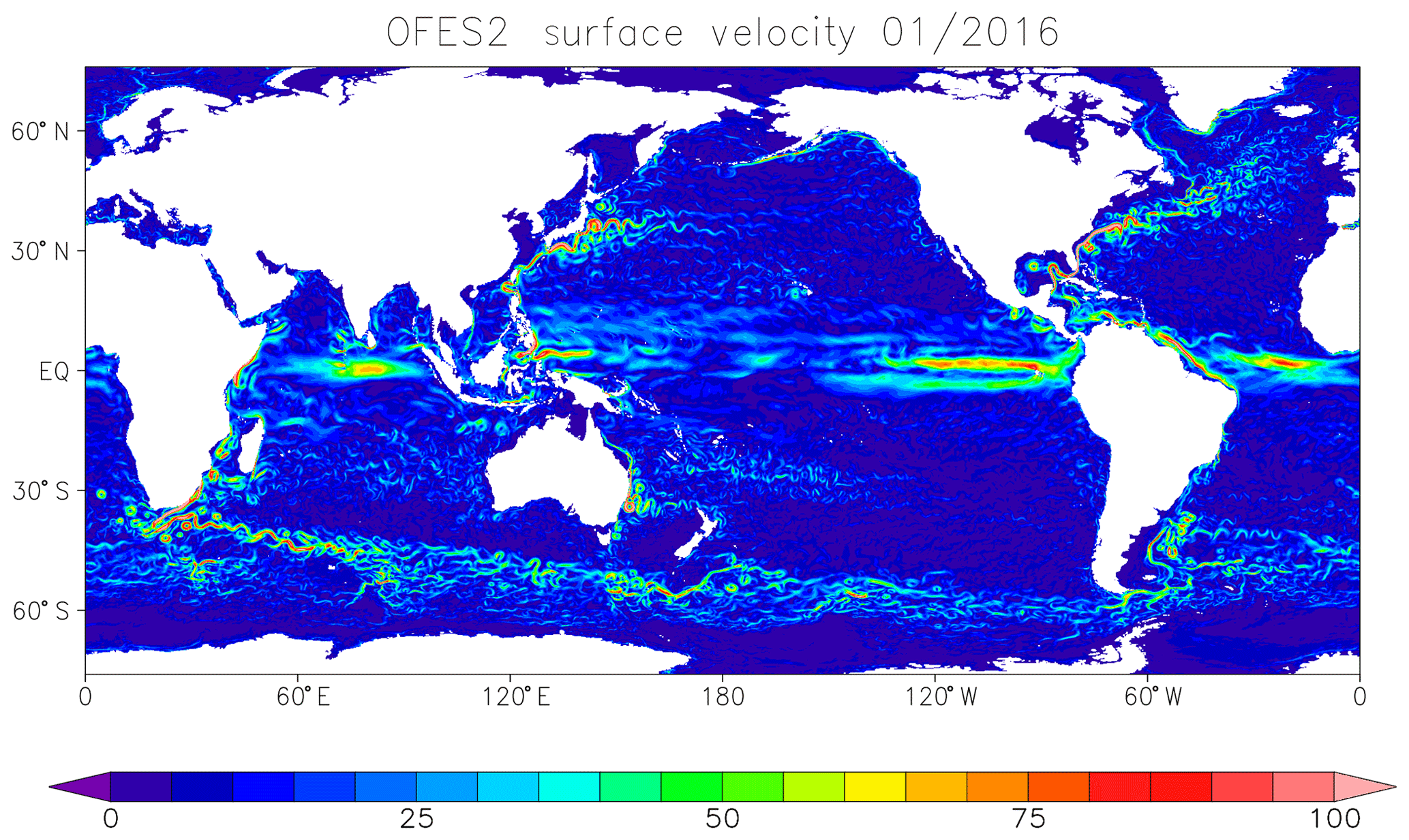
Figure 1An example of monthly averaged surface current speeds (cm s−1) in OFES2.
OFES2 is an update of a quasi-global eddying hindcast simulation: OFES (Sasaki et al., 2008). It is based on the Modular Ocean Model (MOM) version 3 (Pacanowski and Griffies, 1999) and utilizes the latitude and longitude grid system. The horizontal resolution of 0.1∘ remains the same as that in OFES, but the model setup and parameterization are altered to reduce the model biases that exist in OFES. The model configuration of OFES2 will be described first, and the differences from OFES will be described next.
The domain extends from 76∘ S to 76∘ N without polar regions. The horizontal resolution is 0.1∘, and the number of vertical levels is 105 with a maximum depth of 7500 m. The thickness of each layer within the upper 100 m is 5 m. The thickness gradually increases, and there are 55 levels within the upper 500 m. We constructed the bottom topography with partial bottom cells (Adcroft et al., 1997) using the bathymetry dataset ETOPO1 (Amante and Eakins, 2009). Although the model domain does not include the polar regions, a sea-ice model (Komori et al., 2005) was internally implemented into OFES2 to simulate the Antarctic and Subarctic oceans, including the Sea of Okhotsk, more realistically. The sea-ice model employs two-category, zero-layer thermodynamics (Hibler, 1979) and elastic–viscous–plastic rheology (Hunke and Dukowicz, 2002).
A biharmonic operator is used for horizontal mixing to suppress computational noise with a viscosity of 27×109 m4 s−1 and a diffusivity of 9×10⁹ m4 s−1. The drag coefficient is (nondimensional) for linear bottom drag. For vertical mixing, we added diffusivities from the tidal mixing scheme developed by Jayne and St. Laurent (2001) and St. Laurent et al. (2002) to those estimated from the mixed layer vertical mixing scheme of a statistical closure model (Noh and Kim, 1999). In the tidal mixing scheme, the three-dimensional diffusivities are estimated from the energy flux at the ocean bottom and the local buoyancy frequency with the parameters of dissipation efficiency, mixing efficiency, and vertical scale. These parameters are the same as those used by St. Laurent et al. (2002). We used constant barotropic tidal currents of K1 and M2 as the largest diurnal and semidiurnal tidal components in the FES2012 finite-element tide model (Carrère et al., 2012) and the bottom topographic slopes instead of roughness to estimate the energy flux at the ocean bottom (Tanaka et al., 2007). The simulated vertical diffusivities are large over rough bottom topographies and in areas with large tidal motions (Fig. 2a). The diffusivities exponentially decay in the upward direction (e.g., along 10∘ N in Fig. 2b). The distributions of vertical diffusivities in Fig. 2a and b are similar to those of St. Laurent et al. (2002; see their Figs. 1 and 2). The diffusivities do not change much over time because the tidal flow used to estimate the energy flux is assumed to be constant, and therefore the diffusivities change in time only through changes in the local stratification.
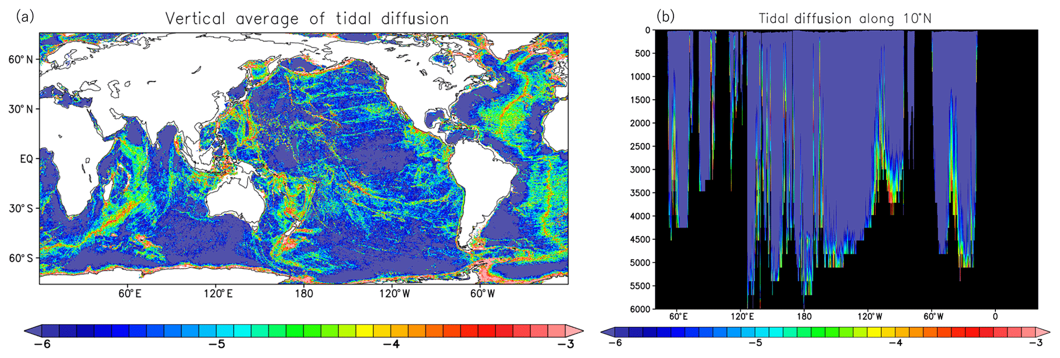
Figure 2Daily mean vertical diffusivity (log10 m2 s−1) on 1 December 2016 estimated by the tidal mixing scheme (a) vertically averaged from the surface to the bottom and (b) in the vertical section along 10∘ N.
We used the 3-hourly atmospheric surface dataset JRA55-do v08 (Tsujino et al., 2018) to estimate surface fluxes in OFES2. This dataset is based on the JRA55 atmospheric reanalysis at a horizontal resolution of approximately 55 km (Kobayashi et al., 2015). Momentum and heat fluxes are calculated with the bulk formulas proposed by Large and Yeager (2004). Note that we used the relative wind speed considering the surface current to estimate the surface momentum flux. We also included the effects of river runoff at river mouths as additional freshwater flux using a monthly mean climatological river runoff dataset from Coordinated Ocean–Ice Reference Experiments (CORE) version 2 (Large and Yeager, 2004). The sea surface salinity (SSS) is restored to monthly climatological values of the WOA13 v2 observations (Zweng et al., 2013) with a 15 d timescale to avoid unrealistic salinity fields.
Since the polar regions are not simulated, the temperature and salinity are restored at all depths to the monthly climatological values from the same WOA13 v2 observations (Locarnini et al., 2013; Zweng et al., 2013) within a distance of 3∘ from the northern and southern boundaries of the model domain. The restoring timescale linearly increases from 1 d at the boundary to infinity at the inner end of the restoring band. Additionally, the temperature and salinity near the straits of Gibraltar, Hormuz, and Bab el Mandeb are restored to observations at all depths since the horizontal resolution of the model is inadequate to capture dynamics within these straits (Fig. 3). The Strait of Gibraltar is where the Mediterranean Sea connects to the Atlantic Ocean, and the straits of Hormuz and Bab el Mandeb are where the Persian Gulf and the Red Sea are connected to the Indian Ocean, respectively.
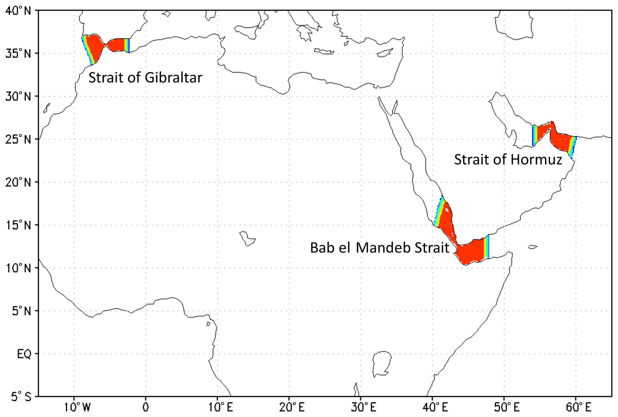
Figure 3Timescales for restoring the temperature and salinity in and near the Straits of Gibraltar, Hormuz, and Bab el Mandeb. Red, yellow, light blue, and blue represent timescales of 1, 5, 10, and 30 d, respectively.
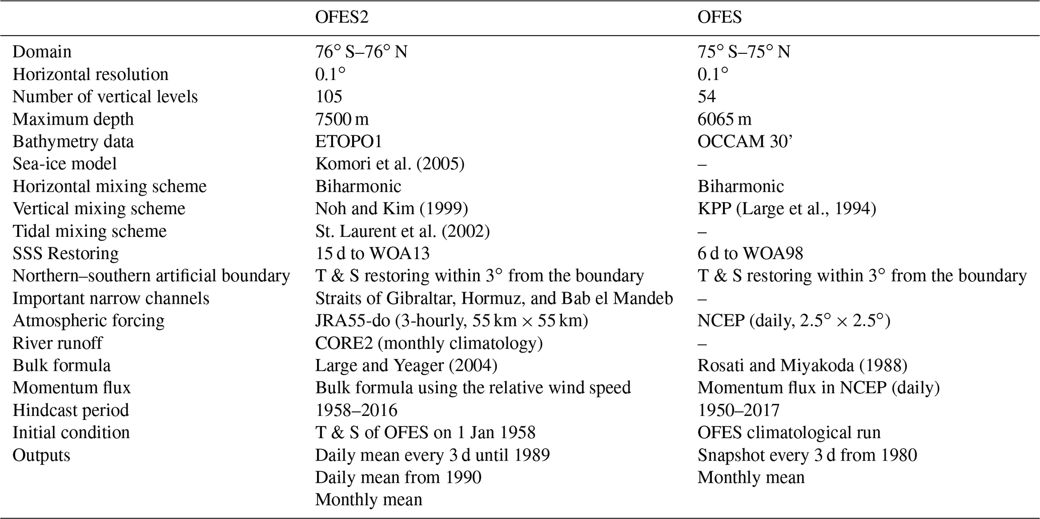
OFES (Sasaki et al., 2008) after 50 years of spin-up integration under climatological forcing (Masumoto et al., 2004) has been integrated from 1950 to the present. OFES2 was integrated from 1958 to 2016 and started with the temperature and salinity fields of OFES from 1 January 1958. Table 1 is the list of the updates for OFES2 compared to OFES. The maximum depth of OFES2 is increased to 7500 from 6065 m. The surface fluxes are now based on 3-hourly data rather than daily data to capture the diurnal cycle. Momentum fluxes are based on a bulk formula using the relative wind speed rather than that estimated in the reanalysis. The distribution of momentum flux curl in OFES2 differs greatly from that in OFES (Fig. S1 in the Supplement). The mixed layer mixing scheme is updated by replacing the K-profile parameterization (KPP) scheme based on an empirical approach (Large et al., 1994) by a statistical closure model (Noh and Kim, 1999). A tidal mixing scheme and a sea-ice model are newly included. The river runoff is also added as additional freshwater flux. SSS is restored with a 15 d timescale rather than a 6 d timescale for the topmost 5 m layer: a 150 d timescale and a 60 d timescale, respectively, for a 50 m mixed layer. The timescale was relaxed compared to OFES, wherein neither sea ice nor river runoff was used.
Table 1Descriptions of the quasi-global eddying hindcast simulations of OFES2 and OFES.
We next discuss improvements in the mean oceanic fields in OFES2 from OFES by comparing those to the observations. The mean temperature and salinity fields at a horizontal resolution of 0.25∘ averaged over 2005–2012 from the World Ocean Atlas 2013 version 2 (WOA13; Locarnini et al., 2013; Zweng et al., 2013) are used, which include a large number of Argo float observations. During this period, both OFES2 and OFES were well spun up. Satellite-observed SSH over 1993–2016 from AVISO is used to examine the simulated oceanic circulations and SSH variations in both OFES2 and OFES. To see how the sea-ice model works in OFES2, the climatological data for sea-ice cover averaged over 2005–2012 from HadISST version 1 (Rayner et al., 2003) are compared with the data in OFES2.
3.1 Global oceanic fields
3.1.1 Sea surface temperature and salinity
Figure 4a and c show the 8-year mean SST and SSS biases averaged over 2005–2012 in OFES2 against WOA13. For SST (Fig. 4a), the bias is less than 1 ∘C in most parts of the globe. Weak cold biases broadly spread over the subtropical Pacific and Indian oceans as well as the Arctic Ocean, and weak warm biases spread over the subarctic Pacific, the subarctic Atlantic, and the Southern Ocean. We also found prominent biases in several regions. Warm biases (>1 ∘C) appear in the South Pacific (170∘–130∘ W and 55∘ S) and to the north of the Kuroshio Extension (140∘–170∘ E and 35∘–40∘ N). In the North Atlantic, along the Gulf Stream and the North Atlantic Current, and in the Labrador and Norwegian seas, several large warm and cold biases (magnitudes larger than 1 ∘C) are present. One possible cause of these biases is the unrealistic current pathway of the Gulf Stream. The Gulf Stream in OFES2 does not turn to the north at approximately 40∘ W, which we will examine more in detail in the next section.
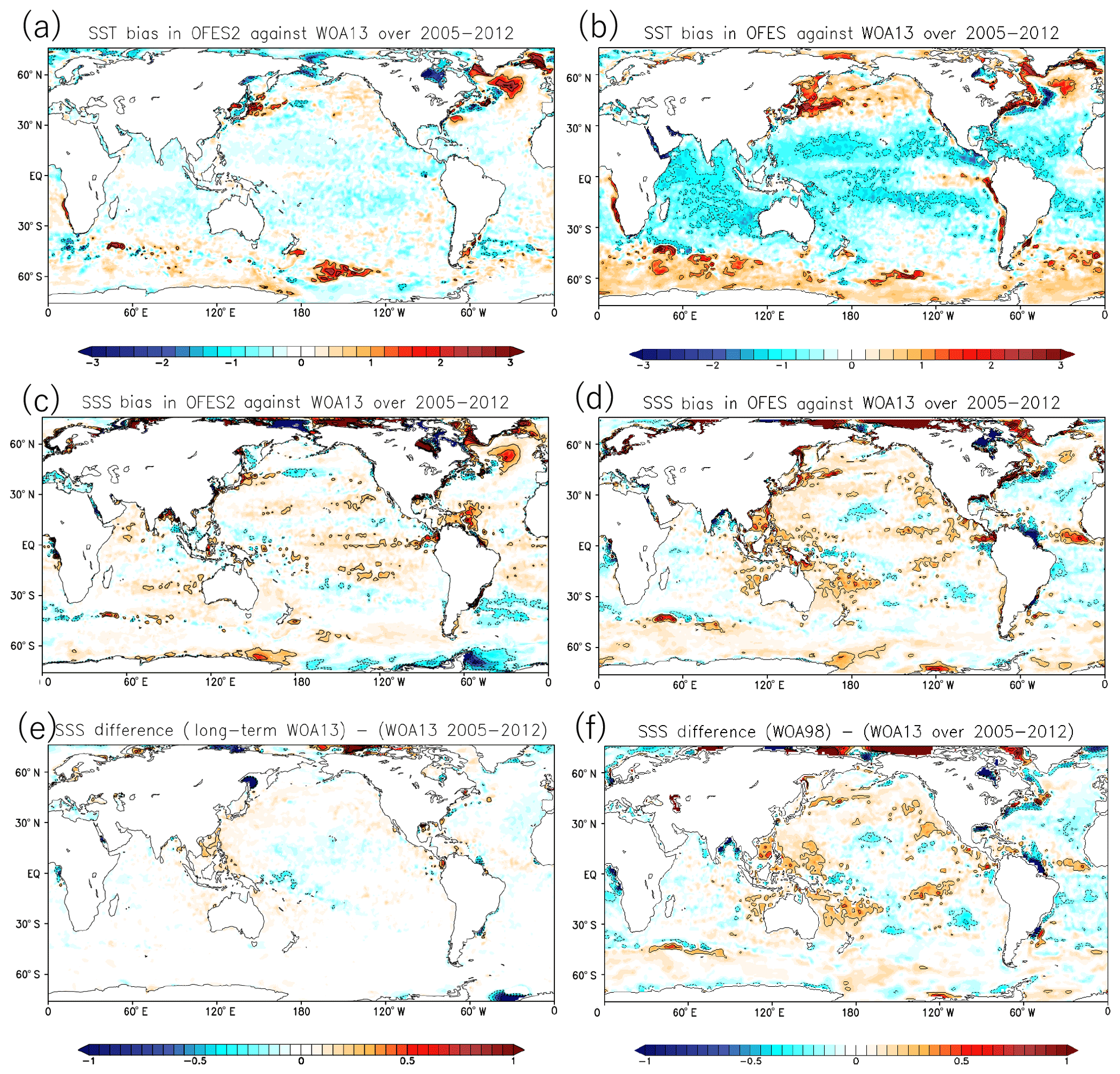
Figure 4SST bias (∘C) in (a) OFES2 and (b) OFES averaged over 2005–2012 against WOA13. Panels (c) and (d) are the same as (a) and (b), respectively, but the SSS bias is shown instead (psu). SSS differences in (e) long-term WOA13 and (f) WOA98 from WOA13 averaged over 2005–2012. The contour lines are superimposed at an interval of 1 ∘C for SST and 0.2 psu for SSS, but zero contour lines are omitted.
The mean SSS biases in OFES2 (Fig. 4c) are smaller than 0.2 psu in most regions. This feature is partly due to the restoring surface boundary condition, but several large biases (larger than 0.2 psu) exist sporadically. The salty bias (>0.4 psu) in the North Atlantic (30∘ W and 50∘ N) likely comes from the unrealistic Gulf Stream pathway, similar to the SST bias mentioned above. The salty bias (>0.4 psu) also appears to the north of South America and in the northern part of the Bay of Bengal. Each salty bias surrounds a fresh bias. One reason for these large salty biases is probably the underestimation of river runoff from the Amazon and Ganges–Brahmaputra rivers, respectively. The impacts of physical processes near the river mouth, such as horizontal and vertical mixing, coastal circulation, and tidal mixing, should also be included to mitigate the biases. In addition, there are large salty and fresh biases in the Chukchi Sea as well as large salty biases in the Nordic and Labrador seas and along the coast of Greenland. These SSS biases are possibly attributed to unrealistic sea-ice distribution in the Chukchi Sea (Fig. 9g) and unrealistic circulations due to the artificial northern boundary.
Figure 4b and d show the 8-year mean SST and SSS biases averaged over 2005–2012 in OFES against WOA13. The SST biases are much smaller in OFES2 (Fig. 4a) than in OFES (Fig. 4b). Cold (warm) SST biases with large amplitudes appear in the equatorial and subtropical regions (high-latitude regions) in both hemispheres in OFES. The centers of the cold biases ( ∘C) zonally spread along 15∘ N and 15∘ S in the Pacific Ocean and the northwestern and southeastern Indian Ocean. Patches of warm biases (>1 ∘C) exist in the Antarctic Ocean to the south of the ACC. Prominent warm biases (>1 ∘C) appear in the northwestern Pacific, the Sea of Okhotsk, and along the west coasts of South America and southern Africa. The prominent warm biases along the west coasts in OFES are presumably associated with unrealistic coastal currents and upwelling, which are driven by unrealistic wind stresses near the coasts in the NCEP reanalysis (Fig. S1). The reductions of these biases in OFES2 are likely a result of using the bulk formula (Large and Yeager, 2004) and the atmospheric surface data (JRA55-do) optimized to drive OGCMs (Tsujino et al., 2018). Additionally, the implementation of a sea-ice model in OFES2 may contribute to the reduction of the warm biases in the Arctic Ocean and the Sea of Okhotsk.
The mean SSS biases in OFES2 (Fig. 4c) are also very reduced compared to those in OFES (Fig. 4d), especially in the tropical and subtropical regions. These bias reductions are also likely due to the bulk formula and atmospheric data used in OFES2. We notice that the global distribution of the biases in OFES (Fig. 4d), prominent in the Arctic Ocean, is quite similar to the difference between WOA98 (Conkright et al., 1998) and WOA13 averaged over 2005–2012 (Fig. 4f). This similarity suggests that the SSS fields in OFES are restored too much toward WOA98. In contrast, the global distribution of the SSS biases in OFES2 (Fig. 4c) does not resemble the difference between long-term mean WOA13 and WOA13 over 2005–2012 (Fig. 4e). The weak restoring in OFES2 does not greatly constrain the simulated SSS. Therefore, the SSS bias in OFES2 (Fig. 4c) comes from something other than the restoring, such as the unrealistic pathways of Kuroshio and the Gulf Stream and the unrealistic sea-ice distribution in the Chukchi Sea as mentioned above.
3.1.2 Sea surface height and its variability
Figure 5 shows the average and standard deviation of the sea surface height (SSH) over 1993–2016 in OFES2, OFES, and AVISO. The large-scale distribution of the mean SSH in OFES2 (Fig. 5a) agrees well with that in AVISO (Fig. 5c), suggesting that OFES2 reproduces the global ocean circulations well. The SSH variability (Fig. 5d) is large around the Gulf Stream, the Kuroshio, and the ACC, which also resembles that in AVISO (Fig. 5f). This large variability is mostly due to high activities of mesoscale eddies and shifts in frontal positions (e.g., Chelton et al., 2007).

Figure 5(a, b, c) Mean SSH (cm) and (d, e, f) its standard deviation (log10 cm) averaged over 1993–2016 from (a, d) OFES2, (b, e) OFES, and (c, f) AVISO observations. The SSH in OFES2 and OFES was offset by adding 50 cm.
However, there are regional differences in the mean SSH distribution and its standard deviation in OFES2 from those in AVISO. The mean SSH contours along the Gulf Stream extend northeastward across the Atlantic in OFES2 (Fig. 5a), while a sharp northern turn is observed at approximately 40∘ W in AVISO (Fig. 5c). The SSH variability is large along the simulated Gulf Stream (Fig. 5d). The zonal extension of the mean SSH contours along with the Azores Current at approximately 33∘ N in the northeastern Atlantic (Fig. 5c) and large SSH variability accompanying this current (Fig. 5f) are recognizable in AVISO but not in OFES2 (Fig. 5a and d). For the Kuroshio in OFES2, the SSH variability is too large along the southern coast of Japan. This large variability is due to the unrealistic detachment of the Kuroshio from Kyushu. Around subtropical countercurrents in the North Pacific and the southern Indian Ocean as well as in most regions away from the strong currents, the SSH variability is slightly smaller in OFES2 than in AVISO. We discuss these issues in Sect. 5.
Compared to OFES (Fig. 5b), the mean SSH in OFES2 (Fig. 5a) shows improvements. In the northern and southern subtropical gyres of the Pacific, the SSH contours are oriented more in the north–south direction in OFES (Fig. 5b) than in OFES2 and AVISO (Fig. 5a and c). In contrast, the improvement in the subtropical gyres of the Atlantic and Indian oceans is limited. One possible cause of this improvement in the SSH field in OFES2 is the replacement of atmospheric wind driving OFES2 by JRA55-do. The overall amplitude of SSH variability around strong currents, such as the Gulf Stream, the Kuroshio, and the ACC, is similar to that of AVISO (Fig. 5f) in OFES2 (Fig. 5d), whereas it is somewhat larger in OFES (Fig. 5e). The northwestward extension of high SSH variability emanating from the southern tip of South Africa, which represents the propagation of Agulhas rings, is too distinct in OFES due to unrealistically long-lived rings. This problem is solved in OFES2. These reductions of SSH variability in OFES2 are possibly due to the eddy-killing effect in the estimation of the surface momentum flux using relative wind (e.g., Renault et al. 2017, 2019a).
3.2 Impact of tidal mixing on water mass property
Internal tides enhance vertical mixing, especially above rough bottom topography. Previous studies have suggested that the Indonesian seas are regions where such mixing significantly impacts the water mass properties (e.g., Ffield and Gordon, 1996). Koch-Larrouy et al. (2007) demonstrated how the inclusion of a local tidal mixing scheme can improve the subsurface water mass in the Indonesian seas and the eastern Indian Ocean. As mentioned in the Introduction, unrealistic water mass properties in the subsurface of Indonesian seas were one of the major biases recognized in OFES (Masumoto et al., 2008), which was one of the motivations to add a tidal mixing scheme in OFES2.
A comparison of subsurface salinity biases in the Indonesian seas shows significant improvement in OFES2 (Fig. 6a and d) from OFES (Fig. 6b and e). The saltier bias at a depth of 135 m is large (>0.5 psu) in the northern Banda Sea in OFES but is greatly reduced in OFES2. To the south of the Sunda Islands, the saltier biases are prominent both at depths of 135 m (>0.2 psu) and 325 m (>0.5 psu) in OFES but are greatly reduced in OFES2. The remaining salty biases in OFES2 may be partially due to a lack of nonlocal tidal mixing (e.g., Nagai et al., 2017), as discussed in Sasaki et al. (2018). This result supports the importance of tidal mixing in the water mass transformation in the Indonesian seas.
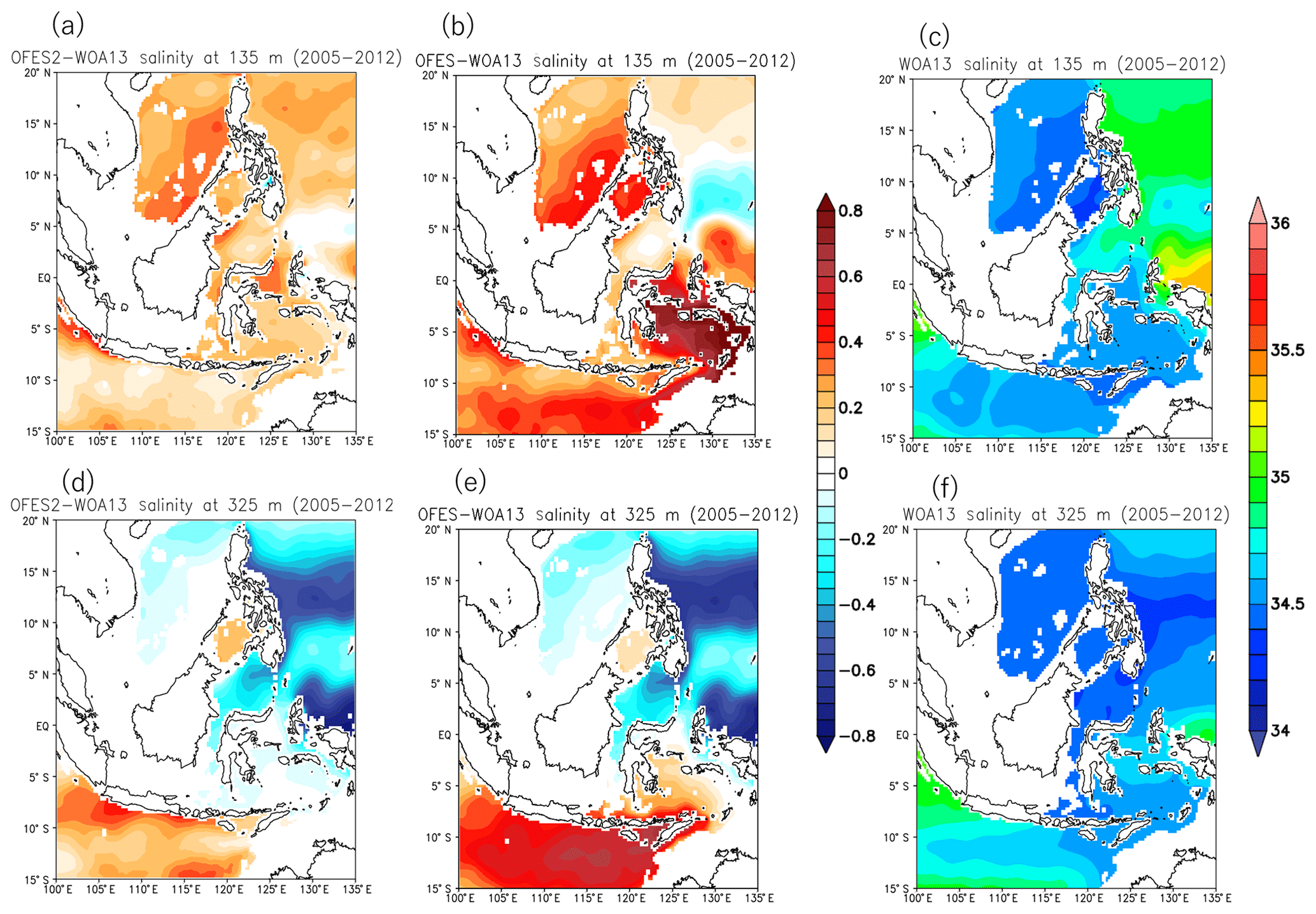
Figure 6Salinity biases (a, b, d, e) against WOA13 (c, f) in OFES2 (a, d) and OFES (b, e) at 135 m (a, b, c) and at 325 m (d, e, f). All fields are averaged over 2005–2012, and the units are practical salinity units (psu).
The Kuril Strait between the North Pacific and the Sea of Okhotsk is another location where previous studies (e.g., Nakamura et al., 2006) have suggested the importance of tidal mixing in the water mass properties of the North Pacific Intermediate Water (NPIW). The vertical section of salinity along 165∘ E in WOA13 shows this subsurface low-salinity water, which OFES reproduces well and OFES2 does a little better (Fig. S2). This result suggests that tidal mixing does not affect the properties of NPIW much, which supports the results using an eddy-permitting model by Tanaka et al. (2010). The vertical diffusivity of 0.02 m2 s−1 used in the strait at all depths in an OGCM in Nakamura et al. (2006) was probably too large.
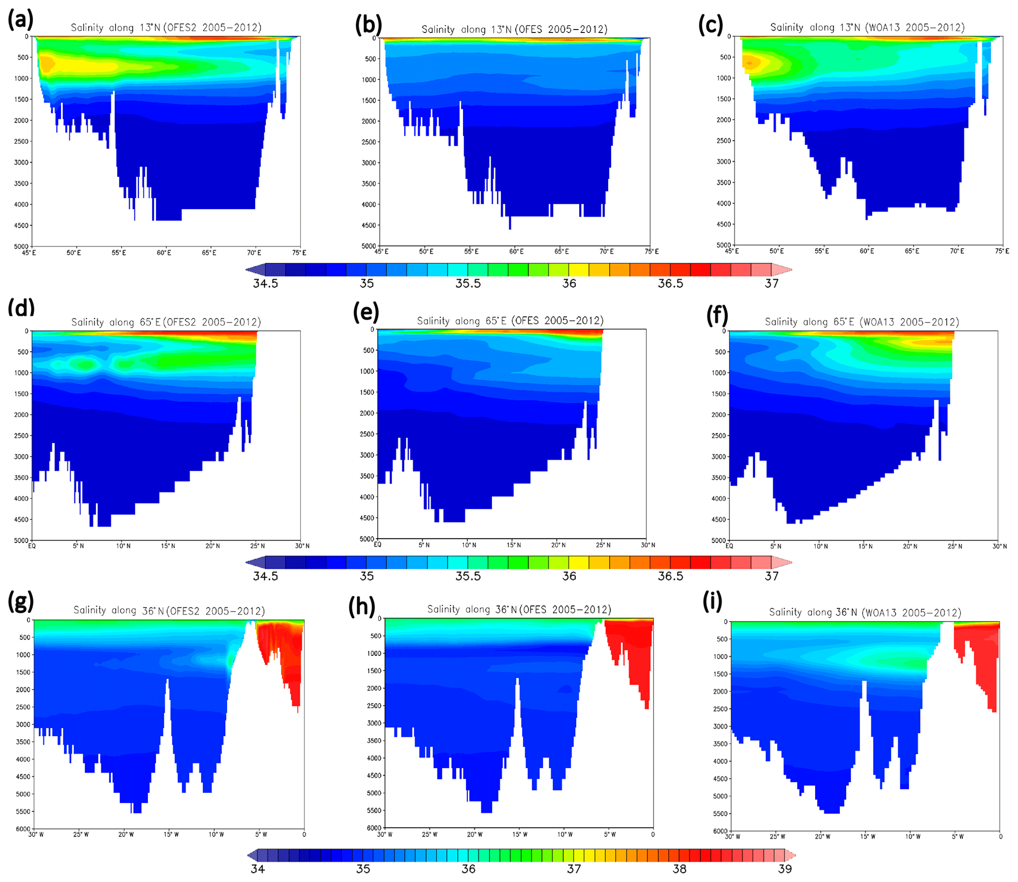
Figure 7Vertical sections of mean salinity along (a–c) 13∘ N and (d–f) 65∘ E in the Arabian Sea and (g–i) 36∘ N in the eastern Atlantic Ocean averaged over 2005–2012: (a, d, g) OFES2, (b, e, h) OFES, and (c, f, i) WOA13.

Figure 8Vertical profile of (a) temperature (∘C) and (b) salinity (psu) at 137∘ E averaged from 8 to 12∘ N and over 2005–2012. (c) Longitudinal distributions of the wind stress curl (10−8 N m−3) along 10∘ N (averaged from 8 to 12∘ N and over 2005–2012). The red, blue, and black curves are OFES2 driven by JRA55-do, OFES driven by the NCEP reanalysis, and the WOA13 observations, respectively.
3.3 Salty outflows from marginal seas
OFES could not accurately simulate high-salinity outflows from the Mediterranean Sea, the Persian Gulf, or the Red Sea to the open ocean. To represent the impacts of these outflows in OFES2, we restored temperature and salinity near the straits (Sect. 2). Proper representations of these outflows are considered important for simulating not only the subsurface but also the surface properties (e.g., Jia, 2000; Prasad et al., 2001; Sofianos and Johns, 2002).
Vertical sections of salinity averaged over 2005–2012 (Fig. 7) exhibit the salty outflows at the subsurface in the Arabian Sea and the Atlantic Ocean. For the Arabian Sea, the basic influence of the outflow appears to be captured in OFES2. The longitudinal section of mean salinity crossing the mouth of the Red Sea shows that OFES2 (Fig. 7a) mostly reproduces the eastward extent of salty water (>35.5 psu) from 46∘ E at approximately 700 m of depth in WOA13 (Fig. 7c). This feature represents the salty outflow from the Red Sea. The eastward extension (>35.5 psu), however, reaches too far to 70∘ E, and its depth of 700 m is too stable over the basin compared to that in WOA13. OFES2 (Fig. 7d) also generally demonstrates the southward spreading of salty outflow from the Persian Gulf: salty water (>35.5 psu) spreads southward from 25∘ N above 1000 m in WOA13 (Fig. 7f). However, the high-salinity core (>35.5 psu) at a depth of 800 m is slightly too distinct and deep in OFES2 (Fig. 7d).
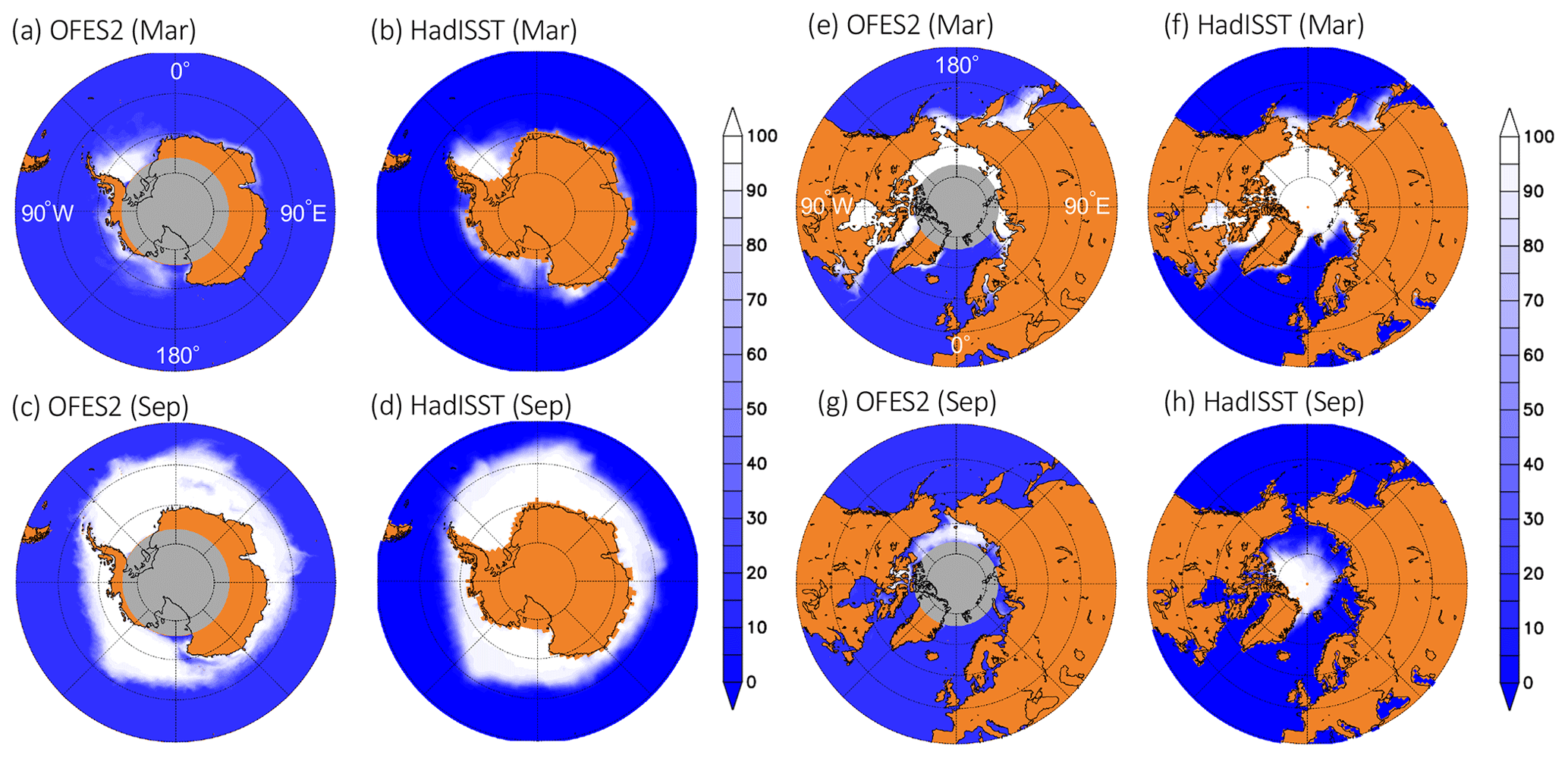
Figure 9Sea-ice concentrations (%) in the Antarctic Ocean in (a, b) March and (c, d) September in (a, c) OFES2 and (b, d) HadISST averaged over 2005–2012. Similarly, the sea-ice concentrations in the Arctic Ocean in (e, f) March and (g, h) September in (e, g) OFES2 and (f, h) HadISST. The gray areas are out of the model domain in OFES2 (a, c, e, g).
In contrast, we found that OFES2 does not reproduce the salty outflow from the Mediterranean Sea into the Atlantic Ocean well, even with the restoration of temperature and salinity near the Strait of Gibraltar. A zonal vertical section of salinity along 36∘ N in the eastern Atlantic Ocean in WOA13 (Fig. 7i) exhibits the westward extension of salty water (>35.8 psu) to 25∘ W at approximately 1100 m of depth and a thick layer with an almost constant salinity of 35.7 psu over 500–1100 m depths to the west of 26∘ W. However, the westward extension of high salinity is weak in OFES2 (Fig. 7g). This high salinity (>36.0 psu) remains to the east of 9∘ W at depths over 1000–1500 m, where OFES2 restores salinity to the observation (Fig. 3). It is not clear why the salty water does not spread westward much in OFES2, but this phenomenon is possibly connected to the bias found in the mid-ocean surface circulation in the North Atlantic (Fig. 5a and c). Entrainment of surface water to the Mediterranean outflow near the Strait of Gibraltar is suggested as the mechanism driving the Azores Current (Jia, 2000; Kida et al., 2008) and the northward turn of the Gulf Stream (Jia, 2000).
The temperature and salinity restoration at the straits resulted in significant improvements in the Arabian Sea from OFES. OFES2 reproduces the salty outflow from the Red Sea well (Fig. 7a) but OFES does not: there is no salty water at the subsurface along 13∘ N in the Arabian Sea (Fig. 7b). OFES2 also greatly improved the salty outflow from the Persian Gulf (Fig. 7d) from OFES (Fig. 7e). The meridional section along 65∘ E shows that the salty subsurface outflow is much fresher by 0.3–0.5 psu in OFES (Fig. 7e) than in WOA13 (Fig. 7f), and its depth of 1000 m is deeper than in WOA13 (800 m). For the Mediterranean outflow, the improvement in OFES2 from OFES is marginal. Both OFES2 (Fig. 7g) and OFES (Fig. 7h) cannot reproduce the westward extent of the salty outflow from the Strait of Gibraltar found in WOA13 (Fig. 7i).
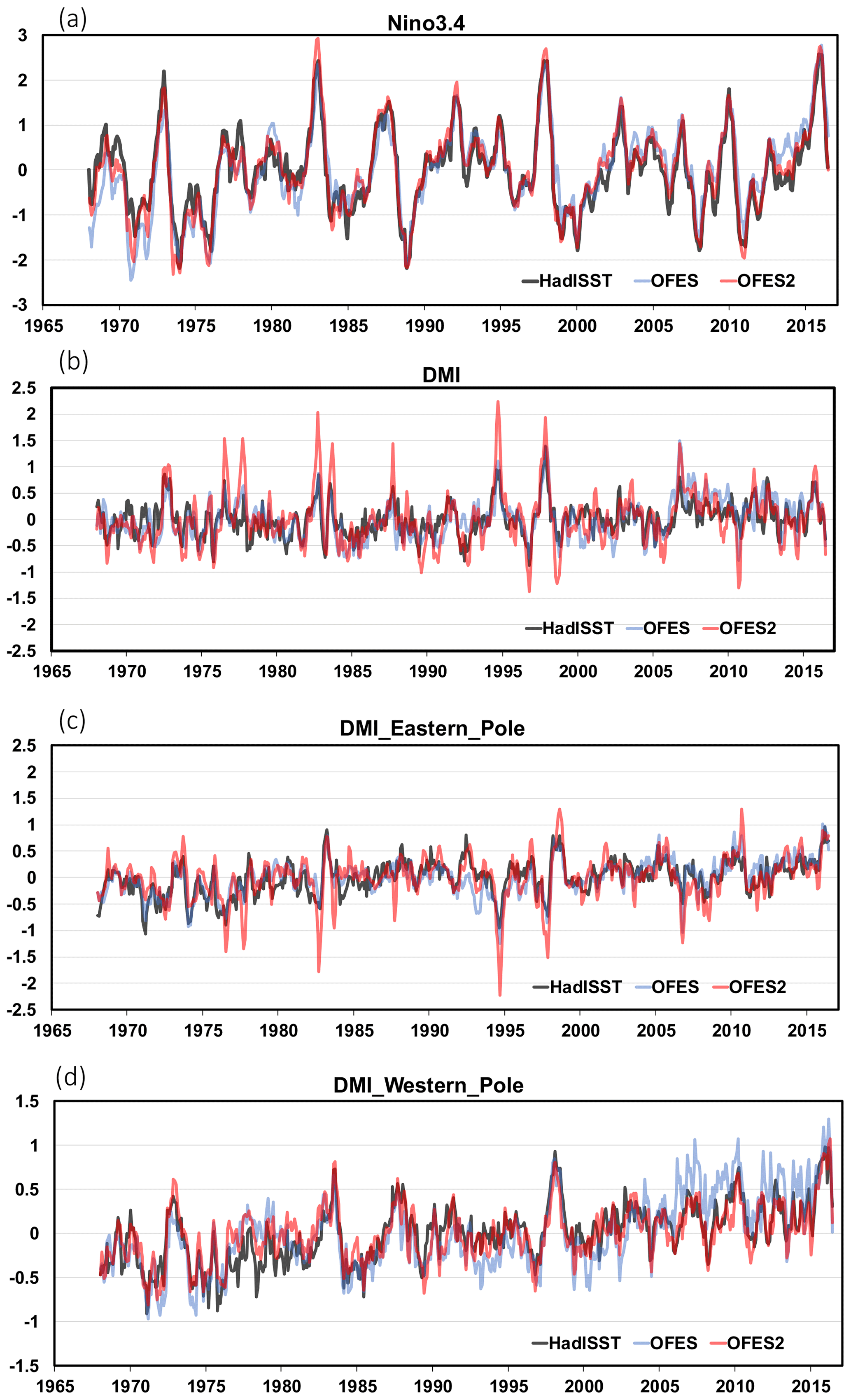
Figure 10(a) Monthly Niño3.4 index defined as SSTAs (∘C) at 165–145∘ W and 5∘ S–5∘ N in the eastern topical Pacific. (b) The monthly DMI (∘C) defined as the difference between the SSTAs (∘C) at the (c) eastern (90–110∘ E, 10∘ S–0∘) and (d) western (50–70∘ E and 10∘ S–10∘ N) poles (Saji et al., 1999) from OFES2 (red curve), OFES (blue curve), and HadISST version 1 (black curve; http://www.cpc.ncep.noaa.gov/data/indices/ last access: 15 July 2020 and http://www.jamstec.go.jp/aplinfo/sintexf/iod/dipole_mode_index.html, last access: 15 July 2020).
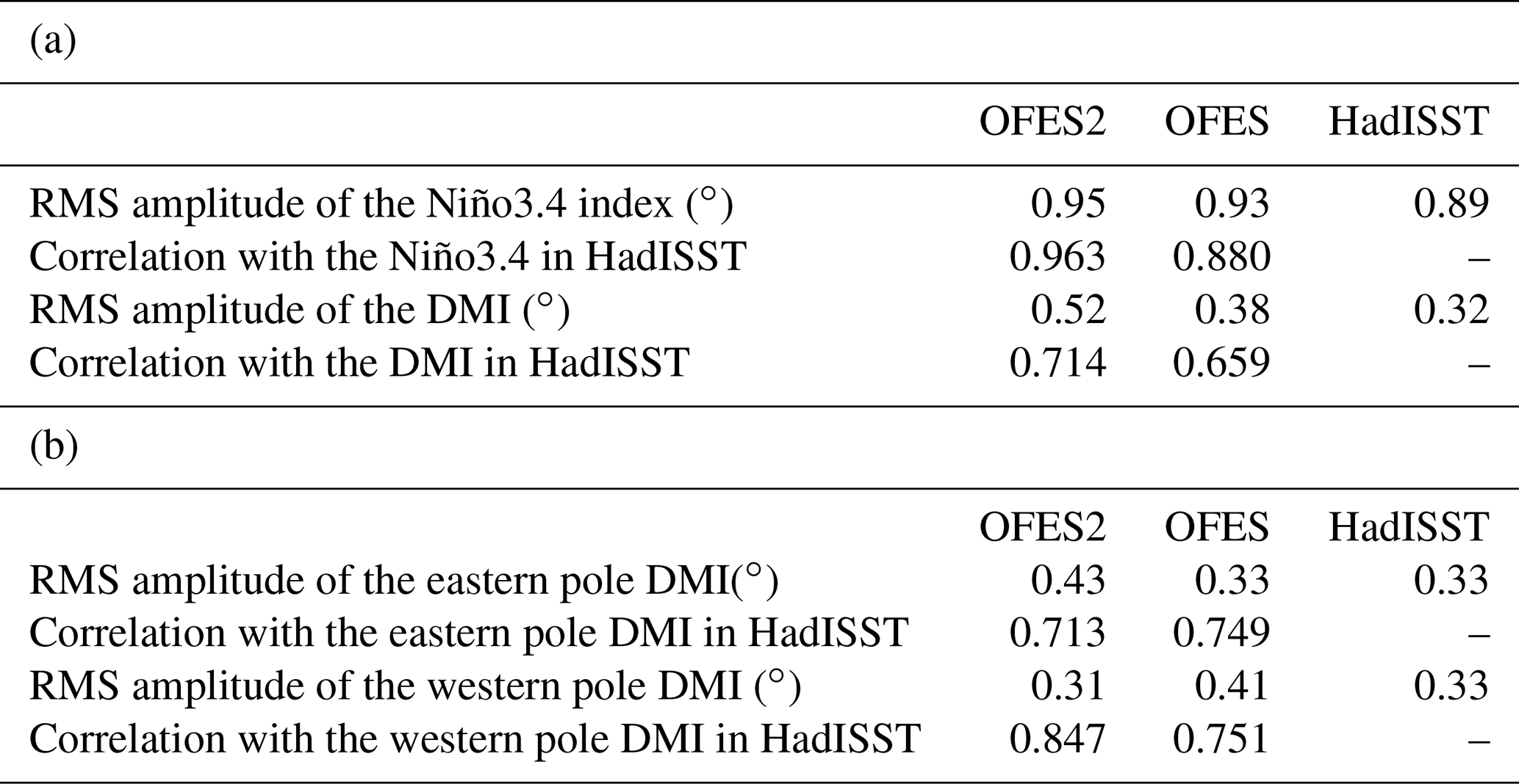
Table 2(a) RMS amplitude (∘C) of the Niño3.4 index and the DMI for OFES2, OFES, and HadISST as well as their correlations between OFES2 and HadISST and between OFES and HadISST. (b) Same as (a) but the eastern and western pole DMIs.
3.4 Subsurface field in the subtropical North Pacific
The subsurface water properties are sensitive to the wind stress product used. Kutsuwada et al. (2019) showed that wind stress products affect the simulated oceanic fields in an OGCM not only at the surface but also in the subsurface. In the subtropical Pacific along 10∘ N, where the subsurface bias is large in OFES (Fig. 4 of Kutsuwada et al., 2019), they found that the use of QuikSCAT wind stress (Kutsuwada, 1998) in another version of OFES, called OFES QSCAT (Sasaki et al., 2006), improves the subsurface water properties compared to OFES, which uses wind stress from the NCEP reanalysis (Kalnay et al., 1996).
The vertical profile of the mean temperatures in the subtropical western Pacific in OFES2 (red curve) mostly overlaps that in WOA13 (black curve) (Fig. 8a). The maximum difference occurs at 280 m and is less than 1 ∘C. This region is characterized by a subsurface salinity maximum (e.g., Nakano et al., 2005). Its depth agrees between OFES2 and WOA13 (Fig. 8b), and its peak salinity value differs a bit by 0.2 psu.
We found that the temperature and salinity biases were significantly reduced in OFES2 from OFES. In the thermocline between 50 and 350 m depths, the temperature is much lower in OFES (Fig. 8a, blue curve) than in WOA13 (black curve). The maximum difference is approximately 6 ∘C at a depth of approximately 150 m. The depth of the salinity maximum is much shallower in OFES (approximately 100 m of depth) than in WOA13 (approximately 140 m of depth) (Fig. 8b). The maximum difference in salinity between OFES and WOA13 is large (∼0.4 psu). These biases are very similar to those found by Kutsuwada et al. (2019) in their comparison between OFES QSCAT and OFES (their Fig. 5). As Kutsuwada et al. (2019) suggested, these large biases in OFES possibly come from wind stress. The wind stress curl used in OFES along 10∘ N (blue curve in Fig. 8c) is relatively strong, which results in the anomalously shallow thermocline via Ekman upwelling that is too large. The wind stress curl in OFES2 (red curve in Fig. 8c) estimated by using 10 m wind in JRA55-do is comparable in amplitudes and variations to the satellite observations (red curve in Fig. 3c of Kutsuwada et al., 2019). The similarity between the wind stress curl in OFES2 and the satellite observations comes from modifications of 10 m wind in JRA55-do using satellite observations (Tsujino et al., 2018).
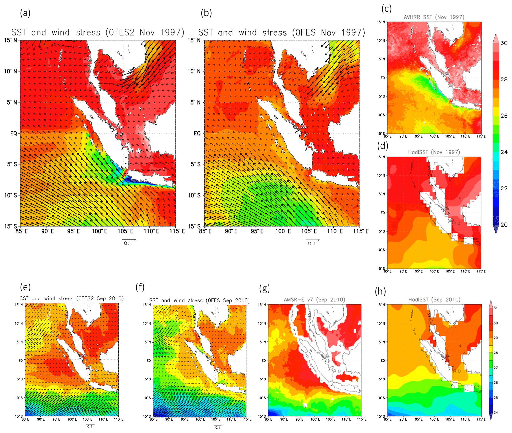
Figure 11SST (∘C) in a region including the IOD eastern pole (90–110∘ E and 10∘ S–0∘) in the mature month of (a–d) the 1997 positive IOD event (November 1997) and (e–h) the 2010 negative IOD event (September 2010). (a, e) OFES2, (b, f) OFES, (c, g) satellite observations of AVHRR version 4.1 (Casey et al., 2010) and AMSR-E version 7 (Wentz and Meissner, 2007), and (d, h) HadISST v1 (Rayner et al., 2003). The vectors in (a, b, e, f) are the surface wind stress (N m−2) in the models, which are plotted at a resolution. The thick vectors denote wind stress magnitudes stronger than 0.05 N m−2.
3.5 Sea-ice distribution in OFES2
We implemented a sea-ice model in OFES2, which is not present in OFES. The domain of OFES2 excludes a large central part of the Arctic Sea and the southernmost parts of the Ross Sea and the Weddell Sea. Figure 9 shows the distribution of monthly climatological sea-ice cover in the polar regions averaged over 2005–2012 compared to the observations from HadISST. The sea-ice cover around Antarctica in March is realistic in OFES2 (Fig. 9a). The simulated sea ice covers most areas of the Weddell Sea, as found in HadISST (Fig. 9b). A small amount of sea ice remains along most of the coastline of East Antarctica in HadISST, whereas OFES2 misses the observed sea-ice cover near the coast from 90 to 180∘ E. The sea-ice cover greatly expands in September compared to March in HadISST (Fig. 9d), and OFES2 reproduces this sea-ice distribution very well (Fig. 9c). Off the coast of Victoria Land between 180 and 150∘ E and along the southern boundary of the model domain (76∘ S) in the Ross Sea (160∘ E–150∘ W), the sea-ice concentration is somewhat lower in OFES2 than in HadISST.
Table 3Improvements in OFES2 over OFES and new or remaining issues in OFES2.

In the Arctic region, the observed sea ice covers the Chukchi Sea in March and seeps into the Bering Sea through the Bering Strait (Fig. 9f). OFES2 reproduces this feature well (Fig. 9e). However, the simulated sea ice spreads too far southward into marginal seas: the Baltic Sea, the Gulf of Saint Lawrence, and the Sea of Okhotsk. In September, unrealistic sea-ice cover spreads in the Chukchi Sea (Fig. 9g), which does not exist in HadISST (Fig. 9h). This discrepancy is possibly due to the artificial northern boundary in OFES2, which blocks the sea-ice outflow through the Fram Strait (Kwok et al., 2004).
Observations show a multi-decadal decreasing trend in summer to fall sea-ice cover in the Arctic region (compare Fig. S3h with Fig. 9h). However, OFES2 fails to capture this trend, probably because of the limited domain, which does not cover most of the Arctic Sea. In the Antarctic region, no comparable trend exists in either OFES2 or observations (Figs. 9a–d, S3a–d).
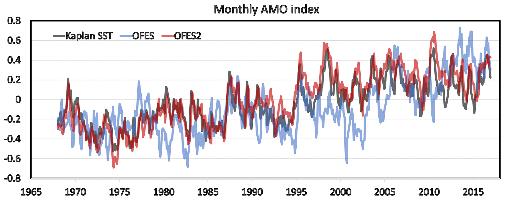
Figure 12Monthly AMO index defined as SSTAs (∘C) at 0∘ S–70∘ N in the eastern topical Pacific in the Kaplan SST (black curve; Kaplan et al., 1998; https://psl.noaa.gov/data/timeseries/AMO/, last access: 15 July 2020), OFES2 (red curve), and OFES (blue curve).
4.1 Niño3.4 and Indian Ocean Dipole mode indexes
We examine the monthly time series of indexes for El Niño and IOD events to determine how well OFES2 reproduces these variations over 1968–2016 (Fig. 10 and Table 2), excluding the initial 10 years to avoid potential impacts of the initial conditions. HadISST version 1 (Rayner et al., 2003) is used as the reference because it covers the whole analysis period. In HadISST, however, the anomalous SST in the eastern pole during the IOD events, which is discussed in Sect. 4.2, appears to be obscure.
The variation in the Niño3.4 index is very similar between OFES2 and HadISST (Fig. 10a). The correlation of the index is very high (0.963), and its root mean square (RMS) amplitude is slightly larger in OFES2 (0.95 ∘C) than in HadISST (0.89 ∘C). For IOD, the Dipole Mode Index (DMI) time series is also similar between OFES2 and HadISST (Fig. 10b). The correlation of the DMI between OFES2 and HadISST is high (0.714), but its RMS amplitude is considerably larger in OFES2 (0.52 ∘C) than in HadISST (0.32 ∘C).
In OFES, the indexes of El Niño and IOD events are also similar to those in HadISST (see Table 2 for the correlations and RMS amplitudes), with somewhat lower correlations than in OFES2. A possible cause of these high correlations in OFES2 is the replacement of the atmospheric dataset by JRA55-do to estimate surface fluxes because usually SST in the ocean models is strongly constrained to the atmospheric data via the surface flux. The RMS amplitudes in OFES (0.93 ∘C for Niño3.4 index and 0.38 ∘C for DMI) are comparable to those of HadISST. The reason why the DMI RMS amplitude is larger in OFES2 (0.52 ∘C) than in OFES or the HadISST (0.32 ∘C) is the variations of the SST anomaly (SSTA) simulated in the eastern pole of the IOD. The SSTA is colder (warmer) in the positive (negative) IOD years of 1982, 1983, 1994, 1997, and 2006 (1996, 1998, and 2010) in OFES2 than in OFES and HadISST (Fig. 10c). The amplitude of SSTA variations is much larger in OFES2 (0.43 ∘C) than in OFES (0.33 ∘C) and HadISST (0.33 ∘C). On the other hand, OFES2 reproduces the time series of SSTA in the western pole well (Fig. 10d), with a correlation coefficient of 0.847 between OFES2 and HadISST compared with 0.751 between OFES and HadISST. In OFES, the SSTA rises greatly after 2005. The amplitude of SSTA variations is similar between OFES2 (0.31 ∘C) and HadISST (0.33 ∘C), which is relatively small compared to OFES (0.41 ∘C). In the next section, we will closely examine this SST distribution around the eastern pole in a typical positive and a typical negative IOD year.
4.2 Sea surface temperature around the eastern pole of the Indian Ocean Dipole
We examine a strong positive and a strong negative IOD event of 1997 and 2010, respectively, as typical cases. Satellite observations captured a low SST (<26 ∘C) area to the southwest of Sumatra and Java during the positive event (Fig. 11c). This anomaly is due to the coastal upwelling induced by anomalous southeasterly wind. OFES2 (Fig. 11a) reproduces this observed anomalously cold SST along the coast well, although the SST near Java is too cold (<22 ∘C). During the negative event, the satellite-observed SST was warm (∼30 ∘C) to the west of Sumatra (Fig. 11g). OFES2 (Fig. 11e) also captures this warm SST well. This warming is presumably due to weak upwelling from weak wind west of Sumatra (Fig. 11e). OFES2 also reproduces cold and warm SST anomalies well at the eastern pole in other IOD events (Fig. S4).
In contrast, HadISST in Fig. 11d (Fig. 11h) does not capture the cold (warm) SST near the southwestern coast of Sumatra and Java in the selected typical positive (negative) IOD event. Therefore, the DMI amplitude from HadISST is likely to be smaller than the reality. In contrast, OISST v2 (Reynolds, 1988), covering a relatively short period from 1981 to the present, reproduces the anomalous SST near the coast well in both the positive and negative IOD events (Fig. S5), which is similar to the satellite observations (Fig. 11c and g). The average amplitude of the DMI over 1981–2016 is 0.54 ∘C for OISST v2, which is comparable to 0.54 ∘C for OFES2. These results suggest that OFES2 reproduces SST anomalies well near the southwestern coast of Sumatra and Java during IOD events and exhibits both the variation and amplitude of the DMI well.
OFES (Fig. 11b) did not accurately reproduce the observed anomalously cold SST (Fig. 11c) near Sumatra and Java during the mature positive IOD event in 1997. The SST in OFES remains unrealistically warm (>26 ∘C) to the southwest of Sumatra and Java. We attribute this fault to the wind stress driving OFES. The strong southeasterly wind stress (thick arrows, >0.05 N m−2) is located far offshore (Fig. 11b), which cannot induce coastal upwelling with realistic strength. On the other hand, the anomalously warm SST at the eastern pole during the negative IOD in 2010 is fairly realistic in OFES (Fig. 11f), although the SST in the entire region is somewhat colder than from the satellite observations (Fig. 11g). This cold SST bias seems consistent with the bias over the entire Indian Ocean in the long-term mean in OFES (Fig. 4b). These features generally apply to other IOD events (Fig. S4). The difference in the SST reproducibility at the eastern pole between the positive and negative events in OFES probably comes from the asymmetric property of the IOD events (e.g., Hong et al., 2008).
This paper describes a new version of our OGCM, which we call OFES2. OFES2 improves the atmospheric forcing to include the diurnal cycle and now includes a tidal mixing scheme and a sea-ice model. We have presented how well OFES2 simulates the mean oceanic features and interannual variations such as El Niño and IOD events, which are generally improved compared to OFES (Table 3).
OFES2 reproduces large-scale circulations and global distributions of mesoscale eddy activity, SST, and SSS well, with significant improvements found in the water mass properties in the subsurface in the subtropical western Pacific and the Arabian and Indonesian seas over OFES. OFES2 also represents the large SSH variability accompanying strong currents well, such as the Gulf Stream and the Kuroshio, whereas SSH variability tends to be somewhat too large in OFES. However, the SSH variability is slightly smaller in most regions in OFES2 than in satellite observations. The surface momentum fluxes in OFES2 are estimated with a bulk formula by using the surface wind relative to the simulated surface current. This method weakens mesoscale eddies, as Zhai and Greatbatch (2007) and Renault et al. (2019a) suggested, which may be the reason for the underestimation of SSH variability in OFES2. Taking into account atmospheric responses to SST gradients, such as impacts on vertical mixing in the atmospheric boundary layer (e.g., Wallace et al., 1989) and pressure adjustment over SST fronts (e.g., Lindzen and Nigam, 1987), in OGCMs may be a solution to overcome this issue. Renault et al. (2019b) also showed the imprints of surface currents on surface atmospheric winds through surface momentum flux in satellite observations and coupled model simulations. The sensitivity of the coupling coefficients (Renault et al., 2020) is an interesting subject for future studies.
The variations of the climate indexes Niño3.4 and DMI are also well simulated in OFES2. The correlations of the monthly indexes between OFES2 and observations are slightly higher than for OFES. During a typical positive IOD event, anomalous southeasterly wind near Sumatra and Java induces cold SSTA via coastal upwelling. OFES2 reproduces this anomalous SST distribution well during typical events, which is due to the realistic surface winds of JRA55-do driving OFES2. Other various climate variations are yet to be examined. As a preliminary exploration, we looked at the Atlantic Multidecadal Oscillation (AMO; Enfield et al., 2001). The monthly AMO index in OFES2 varies with the observation, with a correlation coefficient of 0.90, which is much higher than 0.54 for OFES (Fig. 12).
There are several issues in OFES2 that remain unrealistic from OFES. For example, parts of the pathways of the Kuroshio and Gulf Stream are unrealistic, which created strong SST bias (Fig. 4a and b) and unrealistic SSH variability (Fig. 5d and e) around these currents. We use wind velocity relative to the surface current to estimate the surface momentum fluxes and a deep maximum bottom depth (7500 m), as Tsujino et al. (2013) and Kurogi et al. (2016) did to solve these issues for the Kuroshio. Nevertheless, the simulated Kuroshio in OFES2 frequently makes an unrealistic offshore excursion away from Kyushu. To simulate a realistic Gulf Stream separation, the importance of the sub-grid parameterization (Schoonover et al., 2016), adequate topographic resolution (Schoonover et al., 2017), ageostrophic circulation, and frontogenesis (McWilliams et al., 2019) was suggested. Chassignet and Xu (2017) also succeeded in simulating the separation in a simulation at a horizontal resolution of 1/50∘. In OFES2, the unrealistic pathway of the Gulf Stream contributes mainly to the biases in SST, SSS, and SSH. Sensitivity experiments similar to previous studies are needed to overcome this problem in OFES2.
The Azores Current was also not well simulated even with a restoring condition to reproduce the impact of the salty Mediterranean outflow, which we anticipated driving the Azores Current as suggested by Jia (2000). An interesting result is that the Azores Current and the outflow do exist in the 1960s, but the both abruptly start to decay in the 1970s and disappear after the 1980s (see Figs. S6 and S7 for details). We have not yet found the reason for this behavior.
The impacts of the Mediterranean outflow on deep meridional overturning were also suggested by previous studies (e.g., Reid, 1979; McCartney and Mauitzen 2001). The overturning circulation in the Atlantic Ocean in OFES2 (Fig. S8) appears realistic, but detailed analysis would be necessary to assess the Atlantic circulations over the whole depths. The salty outflows into the Arabian Sea and the water mass properties in the Indonesian seas are improved in OFES2 with the restoring of temperature and salinity near the straits and with the tidal mixing scheme, respectively. There are more issues to investigate, like water mass properties in other regions, in the future.
Another issue in OFES2 is that the domain does not include the polar regions at latitudes higher than 76∘. The sea-ice distribution is unrealistic in the Arctic region (Fig. 9e and g), whose decreasing trend is also not simulated. One possible reason for these defects is the existence of the northern boundary in OFES2 as discussed in Sect. 3.5. The meridional overturning circulations over the globe and in the Atlantic Ocean (Fig. S8) seem reasonable, as mentioned above. A century-scale integration would be necessary to pursue this issue.
The latest supercomputer systems have made possible global eddying ocean simulations with much less computational cost than before. Sensitivity experiments are becoming more feasible. Sasaki et al. (2018) showed that the inclusion of a tidal mixing scheme can result in an enhancement in the transport of Indonesian throughflow due to the basin-scale SSH increase in the tropical Pacific Ocean. While the direct impact of tidal mixing is local, its impact appears to spread over a whole basin via Rossby and Kelvin waves (Furue et al., 2015). Ensemble simulations are another way of utilizing computational power. Nonaka et al. (2016) conducted a three-member ensemble simulation using OFES and suggested the existence of intrinsic variations in the midlatitude ocean currents. One future direction of global, multidecadal, eddying ocean simulations is to obtain a large ensemble.
Global or basin-scale simulations capable of resolving oceanic submesoscales with finer horizontal resolution (e.g., Sasaki et al., 2014; Qiu et al., 2018) are also being pursued. However, it is still difficult to carry out these simulations over many decades due to the huge demands on computational resources and storage. The causes of model biases in eddying simulations are still unresolved, and we still have much to learn from these simulations. Our improved hindcast simulation will be useful for exploring oceanic processes and for Lagrangian analyses of water mass properties (e.g., Kida et al., 2019). We hope that OFES2 will serve as a valuable tool for studying various oceanic features with wide spatiotemporal scales from mesoscale to large-scale circulation and from intraseasonal to decadal timescales.
OFES and OFES2 are based on MOM3, which is available through https://github.com/mom-ocean/MOM3 (last access: 15 July 2020, Pacanowski and Griffies, 1999). The code has been modified for large-scale high-performance simulations and implementations of a sea-ice model and tidal mixing scheme. The modification is copyrighted by the Japan Agency for Marine-Earth Science and Technology (JAMSTEC). The modified code, scripts, and input data to run OFES and OFES2 are available under a copyright agreement. Monthly fields from OFES2 and OFES can be downloaded from JAMSTEC OFES Dataset (https://doi.org/10.17596/0002029, last access: 15 July 2020, Sasaki et al., 2008).
We thank Hiroyuki Tsujino for providing us with the earlier version of the JRA55-do dataset before the official release of the latest version (https://esgf-node.llnl.gov/search/input4mips/, last access: 15 July 2020, Tsujino et al., 2018). The river runoff dataset from CORE version 2 was downloaded from https://data1.gfdl.noaa.gov/nomads/forms/core/COREv2.html (last access: 15 July 2020, Large and Yeager, 2004). The ocean bathymetry from ETOPO1 (https://doi.org/10.7289/V5C8276M, Amante and Eakins, 2009) was used. WOA13 and WOA98 are available at https://www.nodc.noaa.gov/OC5/woa13/ (last access: 15 July 2020, Locarnini et al., 2013; Zweng et al., 2013) and https://www.esrl.noaa.gov/psd/data/gridded/data.nodc.woa98.html (last access: 15 July 2020, Conkright et al., 1998), respectively. HadISST was downloaded from https://www.metoffice.gov.uk/hadobs/hadisst/ (last access: 15 July 2020, Rayner et al., 2003). AMSR-E SST version 7 and AVHRR SST version 4.1 were used through APDRC (http://apdrc.soest.hawaii.edu/, last access: 15 July 2020, Casey et al., 2010). The AMSR data are produced by Remote Sensing Systems and were sponsored by the NASA AMSR-E Science Team and the NASA Earth Science MEaSUREs Program. AVHRR Pathfinder SST was made by GHRSST and the US National Oceanographic Data Center. The AVISO SSH data and FES2012 tidal current speeds were downloaded through AVISO (ftp://ftp-access.aviso.altimetry.fr, last access: 19 October 2019, Carrère et al., 2012). The monthly Niño3.4 index, DMI, and the AMO index were downloaded from http://www.cpc.ncep.noaa.gov/data/indices/ (last access: 15 July 2020, Reynolds, 1988), http://www.jamstec.go.jp/aplinfo/sintexf/iod/dipole_mode_index.html (last access: 15 July 2020, Saji et al., 1999), and https://psl.noaa.gov/data/timeseries/AMO (last access: 15 July 2020, Kaplan et al., 1998, respectively.
The supplement related to this article is available online at: https://doi.org/10.5194/gmd-13-3319-2020-supplement.
HS and SK implemented a tidal scheme, and NK implemented a sea-ice model into OFES2. HS, SK, and RF wrote the paper. HA, YM, TM, MN, YS, and BT contributed model configurations and to writing the paper.
The authors declare that they have no conflict of interest.
OFES and OFES2 simulations were conducted using the Earth Simulator under the support of the Japan Agency for Marine-Earth Science and Technology (JAMSTEC). We thank Takeshi Doi, who provided information about observational data to examine IOD events.
This research has been supported by the Japan Society for the Promotion of Science (JSPS) (KAKENHI grant nos. JP19H05701, JP17K05662, JP18H03731, JP20H01970, JP17K05663, and JP17K05665).
This paper was edited by Qiang Wang and reviewed by two anonymous referees.
Adcroft, A., Hill, C., and Marshall, J.: Representation of topography by shaved cells in a height coordinate ocean model, Mon. Weather Rev., 125, 2293–2315, https://doi.org/10.1175/1520-0493(1997)125<2293:ROTBSC>2.0.CO;2, 1997.
Amante, C. and Eakins, B. W.: ETOPO1 1 arc-minute global relief model: procedures, data sources and analysis, NOAA Technical Memorandum NESDIS NGDC-24, 19 pp., March 2009, available at: http://www.ngdc.noaa.gov/mgg/global/global.html (last access: 15 July 2020), 2009.
Aoki, K., Kubokawa, A., Furue, R., and Sasaki, H.: Influence of eddy momentum fluxes on the mean flow of the Kuroshio Extension in a 1/10∘ Ocean General Circulation Model, J. Phys. Oceanogr., 46, 2769–2784, https://doi.org/10.1175/JPO-D-16-0021.1, 2016.
Carrère, L., Lyard, F., Cancet, M., Guillot, A., and Roblou, L.: FES 2012: a new global tidal model taking advantage of nearly 20 years of altimetry, in: Proceedings of meeting “20 Years of Altimetry”, Venice, 2012.
Chassignet, E. P. and Xu, X.: Impact of horizontal resolution (1/12∘ to 1/50∘) on Gulf Stream separation, penetration, and variability, J. Phys. Oceanogr., 47, 1999–2021, https://doi.org/10.1175/JPO-D-17-0031.1, 2017.
Chassignet, E. P., Hurlburt, H. E., Smedstad, O. M., Halliwell, G. R., Wallcraft, A. J., Metzger, E. J., Blanton B. O., Lozano, C., Rao, D. B., Hogan, P. J., and Srinivasan, A.: Generalized vertical coordinates for eddy-resolving global and coastal ocean forecasts, Oceanography, 19, 118–129, https://doi.org/10.5670/oceanog.2006.95, 2006.
Casey, K. S., Brandon, T. B., Cornillon, P., and Evans, R.: The past, present and future of the AVHRR Pathfinder SST program, in: Oceanography from Space, edited by: Barale, V., Gower, J. F. R., and Alberotanza, L., Springer, https://doi.org/10.1007/978-90-481-8681-5_16, 2010.
Chelton, D. B., deSzoeke, R. A., Schlax, M. G., El Naggar, K., and Siwertz, N.: Geographical variability of the first baroclinic Rossby radius of deformation, J. Phys. Oceanogr., 28, 433–460, https://doi.org/10.1175/1520-0485(1998)028<0433:GVOTFB>2.0.CO;2, 1998.
Chelton, D. B., Schlax, M. G., Samelson, R. M., and de Szoeke, R. A.: Global observations of large oceanic eddies, Geophys. Res. Lett., 34, L15606, https://doi.org/10.1029/2007GL030812, 2007.
Conkright, M. E., Levitus, S., O'Brien, T., Boyer, T. P., Stephens, C., Johnson, D., O. Baranova, Antonov, A., Gelfeld, R., Rochester, J., and Forgy, C.: World Ocean Database 1998 Documentation and Quality Control, National Oceanographic Data Center, Silver Spring, MD, 1998.
Enfield, D. B., Mestas-Nunez, A. M., and Trimble, P. J.: The Atlantic Multidecadal Oscillation and its relationship to rainfall and river flows in the continental U.S., Geophys. Res. Lett., 28, 2077–2080, https://doi.org/10.1029/2000GL012745, 2001.
Ffield, A. and Gordon, A. L.: Tidal mixing signatures in the Indonesian Seas, J. Phys. Oceanogr., 26, 1924–1937, https://doi.org/10.1175/1520-0485(1996)026<1924:TMSITI>2.0.CO;2, 1996.
Furue, R., Jia, Y., McCreary, J. P., Schneider, N., Richards, K. J., Müller, P., Cornuelle, B. D., Avellaneda, N. M., Stammer, D., Liu, C., and Köhld, A.: Impacts of regional mixing on the temperature structure of the equatorial Pacific Ocean. Part 1: Vertically uniform vertical diffusion, Ocean Modell., 91, 91–111, https://doi.org/10.1016/j.ocemod.2014.10.002, 2015.
Hibler III, W. D.: A dynamic thermodynamic sea ice model, J. Phys. Oceanogr., 9, 815–846, https://doi.org/10.1175/1520-0485(1979)009<0815:ADTSIM>2.0.CO;2, 1979.
Hong, C., Li, T., LinHo, and Kug, J.: Asymmetry of the Indian Ocean Dipole. Part I: Observational analysis, J. Climate, 21, 4834–4848, https://doi.org/10.1175/2008JCLI2222.1, 2008.
Hosoda, S., Ohira, T., and Nakamura, T.: A monthly mean dataset of global oceanic temperature and salinity derived from Argo float observations, JAMSTEC Rep. Res. Develop., 8, 47–59, https://doi.org/10.5918/jamstecr.8.47, 2008.
Hu, S., Sprintall, J., Guan, C., Sun, B., Wang, F., Yang, G., Jia, F., Wang, J., Hu, D., and Chai, F.: Spatiotemporal features of intraseasonal oceanic variability in the Philippine Sea from mooring observations and numerical simulations, J. Geophys. Res.-Oceans, 123, 4874–4887, https://doi.org/10.1029/2017JC013653, 2018.
Hunke, E. C. and Dukowicz, J. K.: The elastic–viscous–plastic sea ice dynamics model in general orthogonal curvilinear coordinates on a sphere – Incorporation of metric terms, Mon. Weather Rev., 130, 1848–1865, https://doi.org/10.1175/1520-0493(2002)130<1848:TEVPSI>2.0.CO;2, 2002.
Jayne, S. R. and St. Laurent, L. C.: Parameterizing tidal dissipation over rough topography, Geophys. Res. Lett., 28, 811–814, https://doi.org/10.1029/2000GL012044, 2001.
Jia, Y.: Formation of an Azores Current due to Mediterranean overflow in a modeling study of the North Atlantic, J. Phys. Oceanogr., 30, 2342–2358, https://doi.org/10.1175/1520-0485(2000)030<2342:FOAACD>2.0.CO;2, 2000.
Jungclaus, J. H., Fischer, N., Haak, H., Lohmann, K., Marotzke, J., Matei, D., Mikolajewicz, U., Notz, D., and Storch, J. S.: Characteristics of the ocean simulations in MPIOM, the ocean component of the MPI-Earth system model, J. Adv. Model. Earth Syst., 5, 422–446, https://doi.org/10.1002/jame.20023, 2013.
Kalnay, E., Kanamitsu, M., Kistler, R., Collins, W., Deaven, D., Gandin, L., Iredell, M., Saha, S., White, G., Woollen, J., Zhu, Y., Chelliah, M., Ebisuzaki, W., Higgins, W., Janowiak, J., Mo, K. C., Ropelewski, C., Wang, J., Leetmaa, A., Reynolds, R., Jenne, R., and Joseph, D.: The NCEP/NCAR 40-year reanalysis project, B. Am. Meteorol. Soc., 77, 437–471, https://doi.org/10.1175/1520-0477(1996)077<0437:TNYRP>2.0.CO;2, 1996.
Kaplan, A., Cane, M., Kushnir, Y., Clement, A., Blumenthal, M., and Rajagopalan, B.: Analyses of global sea surface temperature 1856–1991, J. Geophys. Res., 103, 18567–18589, https://doi.org/10.1029/97JC01736, 1998.
Kida, S., Price, J. F., and Yang, J.: The upper-oceanic response to overflows: A mechanism for the Azores Current, J. Phys. Oceanogr., 38, 880–895, https://doi.org/10.1175/2007JPO3750.1, 2008.
Kida, S., Richards, K. J., and Sasaki, H.: The fate of surface freshwater entering the Indonesian Seas, J. Geophys. Res.-Oceans, 124, 3228–3245, https://doi.org/10.1029/2018JC014707, 2019.
Kobayashi, S., Ota, Y., Harada, Y., Ebita, A., Moriya, M., Onoda, H., Onogi, K., Kamahori, H., Kobayashi, C., Endo, H., Miyaoka, K., and Takahashi, K.: The JRA-55 reanalysis: General specifications and basic characteristics, J. Meteorol. Soc. JPN Ser. II, 93, 5–48, https://doi.org/10.2151/jmsj.2015-001, 2015.
Koch-Larrouy, A., Madec, G., Bouruet-Aubertot, P., Gerkema, T., Bessières, L., and Molcard, R.: On the transformation of Pacific Water into Indonesian Throughflow Water by internal tidal mixing, Geophys. Res. Lett., 34, L04604, https://doi.org/10.1029/2006GL028405, 2007.
Komori, N., Takahashi, K., Komine, K., Motoi, T., Zhang, X., and Sagawa, G.: Description of sea-ice component of Coupled Ocean Sea-Ice Model for the Earth Simulator (OIFES), J. Earth Simulator, 4, 31–45, https://doi.org/10.32131/jes.4.31, 2005.
Kurogi, M., Tanaka, Y., and Hasumi, H.: Effects of deep bottom topography on the Kuroshio Extension studied by a nested-grid OGCM, CLVAR Exchanges, 69, 19–21, 2016.
Kutsuwada, K.: Impact of wind/wind-stress field in the North Pacific constructed by ADEOS/NSCAT data, J. Oceanogr., 54, 443–456, https://doi.org/10.1007/BF02742447, 1998.
Kutsuwada, K., Kakiuchi, A., Sasai, Y., and Sasaki, H.: Wind-driven North Pacific Tropical Gyre using high-resolution simulation outputs, J. Oceanogr., 75, 81–93, https://doi.org/10.1007/s10872-018-0487-8, 2019.
Kwok, R., Cunningham, G. F., and Pang, S. S.: Fram Strait sea ice outflow, J. Geophys. Res., 109, C01009, https://doi.org/10.1029/2003JC001785, 2004.
Large, W. and Yeager, S.: Diurnal to decadal global forcing for ocean and sea-ice models: The data sets and flux climatologies, NCAR Technical Note NCAR/TN-460+STR, https://doi.org/10.5065/D6KK98Q6, 2004.
Large, W. G., McWilliams, J. C., and Doney, S. C.: Oceanic vertical mixing: A review and a model with a nonlocal boundary layer parameterization, Rev. Geophys., 32, 363–403, https://doi.org/10.1029/94RG01872, 1994.
Lindzen, R. S. and Nigam, S.: On the role of sea surface temperature gradients in forcing low-level winds and convergence in the tropics, J. Atmos. Sci., 44, 2418–2436, https://doi.org/10.1175/1520-0469(1987)044<2418:OTROSS>2.0.CO;2, 1987.
Locarnini, R. A., Mishonov, A. V., Antonov, J. I., Boyer, T. P., Garcia, H. E., Baranova, O. K., Zweng, M. M., Paver, C. R., Reagan, J. R., Johnson, D. R., Hamilton, M., and Seidov, D.: World Ocean Atlas 2013, Volume 1: Temperature, edited by: Levitus, S., A. Mishonov Technical Ed., NOAA Atlas NESDIS 73, 40 pp., https://doi.org/10.7289/V55X26VD, 2013.
Maltrud, M. E. and McClean, J. L.: An eddy resolving global 1/10∘ ocean simulation, Ocean Modell., 8, 31–54, https://doi.org/10.1016/j.ocemod.2003.12.001, 2005.
Masumoto, Y.: Sharing the results of a high-resolution ocean general circulation model under a multi-discipline framework – a review of OFES activities, Ocean Dynam., 60, 633–652, https://doi.org/10.1007/s10236-010-0297-z, 2010.
Masumoto, Y., Sasaki, H., Kagimoto, T., Komori, N., Ishida, A., Sasai, Y., Miyama, T., Motoi, T., Mitsudera, H., Takahashi, k., Sakuma, H., and Yamagata, T.: A fifty-year eddy-resolving simulation of the world ocean – Preliminary outcomes of OFES (OGCM for the Earth Simulator), J. Earth Simulator, 1, 35–56, https://doi.org/10.32131/jes.1.35, 2004.
Masumoto, Y., Morioka, Y., and Sasaki, H.: High-resolution Indian Ocean simulations – Recent advances and issues from OFES-, in: Ocean Modeling in an Eddying Regime, edited by: Hecht, M. W., Hasumi, H., Geophysical Monograph Series, 177, AGU, Washington D.C., 165–175, https://doi.org/10.1029/177GM14, 2008.
McCartney, M. S. and Mauritzen, C.: On the origin of the warm inflow to the Nordic Seas, Prog. Oceanogr., 51, 125–214, https://doi.org/10.1016/S0079-6611(01)00084-2, 2001.
McWilliams, J. C., Gula, J., and Molemaker, M. J.: The Gulf Stream North wall: Ageostrophic circulation and frontogenesis, J. Phys. Oceanogr., 49, 893–916, https://doi.org/10.1175/JPO-D-18-0203.1, 2019.
Nagai, T., Hibiya, T., and Bouruet-Aubertot, P.: Nonhydrostatic simulations of tide-induced mixing in the Halmahera Sea: A possible role in the trans formation of the Indonesian Throughflow waters, J. Geophys. Res.-Oceans, 122, 8933–8943, https://doi.org/10.1002/2017JC013381, 2017.
Nakamura, T., Toyoda, T., Ishikawa, Y., and Awaji, T.: Enhanced ventilation in the Okhotsk Sea through tidal mixing at the Kuril Straits, Deep Sea Res. PT I, 53, 425–448, https://doi.org/10.1016/j.dsr.2005.12.006, 2006.
Nakano, T., Kitamura, T., Sugimoto, S., Suga, T., and Kamachi, M.: Long-term variations of North Pacific Tropical Water along the 137∘ E repeat hydrographic section, J. Oceanogr., 71, 229–238, https://doi.org/10.1007/s10872-015-0279-3, 2005.
Noh, Y. and Kim, H. J.: Simulations of temperature and turbulence structure of the oceanic boundary layer with the improved near-surface process, J. Geophys. Res., 104, 15621–15634, https://doi.org/10.1029/1999JC900068, 1999.
Nonaka, M., Sasai, Y., Sasaki, H., Taguchi, B., and Nakamura, H.: How potentially predictable are midlatitude ocean currents?, Sci. Rep., 6, 20153, https://doi.org/10.1038/srep20153, 2016.
Pacanowski, R. C. and Griffies, S. M.: The MOM3 manual. GFDL Ocean Group Tech. Rep. 4, NOAA. Geophysical Fluid Dynamics Laboratory, Princeton, NJ., available at: https://mdl-mom5.herokuapp.com/web/docs/project/MOM3_manual.pdf (last access: 20 July 2020), 1999.
Prasad, T. G., Ikeda, M., and Kumar, S. P.: Seasonal spreading of the Persian Gulf Water mass in the Arabian Sea, J. Geophys. Res.-Oceans, 106, 17059–17071, https://doi.org/10.1029/2000JC000480, 2001.
Qiu, B. and Chen, S.: Eddy-mean flow interaction in the decadally-modulating Kuroshio Extension system, Deep Sea Res. Pt. II, 57, 1098–1110, https://doi.org/10.1016/j.dsr2.2008.11.036, 2010.
Qiu, B., Chen, S., Klein, P., Wang, J., Torres, H., Fu, L., and Menemenlis, D.: Seasonality in transition scale from balanced to unbalanced motions in the world ocean, J. Phys. Oceanogr., 48, 591–605, https://doi.org/10.1175/JPO-D-17-0169.1, 2018.
Rayner, N. A., Parker, D. E., Horton, E. B., Folland, C. K., Alexander, L. V., Rowell, D. P., Kent, E. C., and Kaplan, A.: Global analyses of sea surface temperature, sea ice, and night marine air temperature since the late nineteenth century, J. Geophys. Res.-Atmos., 108, 4407, https://doi.org/10.1029/2002JD002670, 2003.
Reid, J. L.: On the contribution of the Mediterranean Sea outflow to the Norwegian-Greenland Sea, Deep Sea Res. A, 26, 1199–1223, https://doi.org/10.1016/0198-0149(79)90064-5, 1979.
Renault, L., McWilliams, J. C., and Penven, P.: Modulation of the Agulhas current retroflection and leakage by oceanic current interaction with the atmosphere in coupled Simulations, J. Phys. Oceanogr., 47, 2077–2100, https://doi.org/10.1175/JPO-D-16-0168.1, 2017.
Renault, L., Marchesiello, P., Masson, S., and McWilliams, J. C.: Remarkable control of western boundary currents by eddy killing, a mechanical air-sea coupling process, Geophys. Res. Lett., 46, 2743–2751, https://doi.org/10.1029/2018GL081211, 2019a.
Renault, L., Masson, S., Oerder, V., Jullien, S., and Colas, F.: Disentangling the mesoscale ocean-atmosphere interactions, J. Geophys. Res.-Oceans, 124, 2164–2178, https://doi.org/10.1029/2018JC014628, 2019b.
Renault, L., Masson, S., Arsouze, T., Madec, G., and McWilliams, J. C.: Recipes for how to force oceanic model dynamics, J. Adv. Mod. Ear. Sys., 12, e2019MS001715, https://doi.org/10.1029/2019MS001715, 2020.
Reynolds, R. W.: A real-time global sea surface temperature analysis, J. Climate, 1, 75–86, https://doi.org/10.1175/1520-0442(1988)001<0075:ARTGSS>2.0.CO;2, 1988.
Roemmich, D., Johnson, G., Riser, S., Davis, R., Gilson, J., Owens, W. B., Garzoli, S. L., Schmid, C., and Ignaszewski, M.: The Argo program: Observing the global ocean with profiling floats, Oceanography, 22, 34–43, https://doi.org/10.5670/oceanog.2009.36, 2009.
Rosati, A. and Miyakoda, K.: A general circulation model for upper ocean circulation, J. Phys. Oceanogr., 18, 1601–1626, https://doi.org/10.1175/1520-0485(1988)018<1601:AGCMFU>2.0.CO;2, 1988.
Saji, N. H., Goswami, B. N., Vinayachandran, P. N., and Yamagata, T.: A dipole mode in the tropical Indian Ocean, Nature, 401, 360–363, https://doi.org/10.1038/43854, 1999.
Sasaki, H., Sasai, Y., Nonaka, M., Masumoto, Y., and Kawahara, S.: An eddy-resolving simulation of the quasi-global ocean driven by satellite-observed wind field: Preliminary outcomes from physical and biological fields, J. Earth Simulator, 6, 35–49, https://doi.org/10.32131/jes.6.35, 2006.
Sasaki, H., Nonaka, M., Masumoto, Y., Sasai, Y., Uehara, H., and Sakuma, H.: An eddy-resolving hindcast simulation of the quasiglobal ocean from 1950 to 2003 on the Earth Simulator, edited by: Hamilton, K. and Ohfuchi, W., High Resolution Numerical Modelling of the Atmosphere and Ocean, Springer, New York, NY, 157–186, https://doi.org/10.1007/978-0-387-49791-4_10, 2008.
Sasaki, H., Klein, P., Qiu, B., and Sasai, Y.: Impact of oceanic scale-interactions on the seasonal modulation of ocean dynamics by the atmosphere, Nat. Commun., 5, 5636, https://doi.org/10.1038/ncomms6636, 2014.
Sasaki, H., Kida, S., Furue, R., Nonaka, M., and Masumoto, Y.: An increase of the Indonesian Throughflow by internal tidal mixing in a high-resolution quasi-global ocean simulation, Geophys. Res. Lett., 45, 8416–8424, https://doi.org/10.1029/2018GL078040, 2018.
Sasaki, Y. N. and Schneider, N.: Decadal shifts of the Kuroshio Extension jet: application of thin–jet theory, J. Phys. Oceanogr., 41, 979–993, https://doi.org/10.1175/2011JPO4550.1, 2011.
Schoonover, J., Dewar, W., Wienders, N., Gula, J., McWilliams, J.C., Molemaker, M. J., Bates, S. C., Danabasoglu, G., and Yeager, S.: North Atlantic barotropic vorticity balances in numerical models, J. Phys. Oceanogr., 46, 289–303, https://doi.org/10.1175/JPO-D-15-0133.1, 2016.
Schoonover, J., Dewar, W., Wienders, N., and Deremble, B.: Local sensitivities of the Gulf Stream separation, J. Phys. Oceanogr., 47, 353–373, https://doi.org/10.1175/JPO-D-16-0195.1, 2017.
Sofianos, S. S. and Johns, W. E.: An Oceanic General Circulation Model (OGCM) investigation of the Red Sea circulation, 1, Exchange between the Red Sea and the Indian Ocean, J. Geophys. Res.-Oceans, 107, 3196, https://doi.org/10.1029/2001JC001184, 2002.
St. Laurent, L. C., Simmons, H. L., and Jayne, S. R.: Estimating tidally driven mixing in the deep ocean, Geophys. Res. Lett., 29, 2106, https://doi.org/10.1029/2002GL015633, 2002.
Taguchi, B., Schneider, N., Nonaka, M, and Sasaki, H.: Decadal variability of upper-ocean heat content associated with meridional shifts of western boundary current extensions in the North Pacific, J. Climate, 30, 6247–6264, https://doi.org/10.1175/JCLI-D-16-0779.1, 2017.
Tanaka, Y., Hibiya, T., and Niwa, Y.: Estimates of tidal energy dissipation and diapycnal diffusivity in the Kuril Straits using TOPEX/POSEIDON altimeter data, J. Geophys. Res.-Oceans, 112, C10021, https://doi.org/10.1029/2007JC004172, 2007.
Tanaka, Y., Hibiya, T., and Niwa, Y.: Assessment of the effects of tidal mixing in the Kuril Straits on the formation of the North Pacific Intermediate Water, J. Phys. Oceanogr., 40, 2569–2574, https://doi.org/10.1175/2010JPO4506.1, 2010.
Tsujino, H., Nishikawa, S., Sakamoto, K., Usui, N., Nakano, H., and Yamanaka, G.: Effects of large-scale wind on the Kuroshio path south of Japan in a 60-year historical OGCM simulation, Clim. Dynam., 41, 2287–2318, https://doi.org/10.1007/s00382-012-1641-4, 2013.
Tsujino, H., Urakawa, S., Nakano, H., Small, R. J., Kim, W. M., Yeager, S. G., Danabasoglu, G., Suzuki, T., Bamber, J. L., Bentsen, M., Böning, C. W., Bozec, A., Chassignet, E. P., Curchitser, E., Dias, F. B., Durack, P. J., Griffies, S. M., Harada, Y., Ilicak, M., Josey, S. A., Kobayashi, C., Kobayashi, S., Komuro, Y., Large, W. G., Le Sommer, J., Marsland, S. J., Masina, S., Scheinert, M., Tomita, H., Valdivieso, M., and Yamazaki, D.: JRA-55 based surface dataset for driving ocean–sea-ice models (JRA55-do), Ocean Modell., 130, 79–139, https://doi.org/10.1016/j.ocemod.2018.07.002, 2018.
Wallace, J. M., Michell, T. P., and Deser, C.: The influence of sea-surface temperature on surface wind in the eastern equatorial Pacific: Seasonal and interannual variability, J. Climate, 2, 1492–1499, https://doi.org/10.1175/1520-0442(1989)002<1492:TIOSST>2.0.CO;2, 1989.
Wentz, F. J. and Meissner, T.: Supplement 1: Algorithm theoretical basis document for AMSR-E ocean algorithms, Remote Sensing Systems Tech. Rep. 051707, 6 pp., https://ghrc.nsstc.nasa.gov/opendap/tpw/doc/AMSR_Ocean_Algorithm_Version_2_Supplement_1.pdf (last access: 15 July 2020), 2007.
Zhai, X. and Greatbatch, R. J.: Wind work in a model of the northwest Atlantic Ocean, Geophys. Res. Lett., 34, L04606, https://doi.org/10.1029/2006GL028907, 2007.
Zhai, X., Greatbatch, R. J., and Kohlmann, J. D.: On the seasonal variability of eddy kinetic energy in the Gulf Stream region, Geophys. Res. Lett., 35, L24609, https://doi.org/10.1029/2008GL036412, 2008.
Zweng, M. M., Reagan, J. R., Antonov, J. I., Locarnini, R. A., Mishonov, A. V., Boyer, T. P., Garcia, H. E., Baranova, O. K., Johnson, D. R., Seidov, D., and Biddle, M. M.: World Ocean Atlas 2013, Volume 2: Salinity. S. Levitus, Ed., A. Mishonov Technical Ed.; NOAA Atlas NESDIS 74, 39 pp., https://doi.org/10.7289/V5251G4D, 2013.