the Creative Commons Attribution 4.0 License.
the Creative Commons Attribution 4.0 License.
 | 31 Jan 2020
CobWeb 1.0: machine learning toolbox for tomographic imaging
Swarup Chauhan
Kathleen Sell
Wolfram Rühaak
Thorsten Wille
Ingo Sass
Despite the availability of both commercial and open-source software, an ideal tool for digital rock physics analysis for accurate automatic image analysis at ambient computational performance is difficult to pinpoint. More often, image segmentation is driven manually, where the performance remains limited to two phases. Discrepancies due to artefacts cause inaccuracies in image analysis. To overcome these problems, we have developed CobWeb 1.0, which is automated and explicitly tailored for accurate greyscale (multiphase) image segmentation using unsupervised and supervised machine learning techniques. In this study, we demonstrate image segmentation using unsupervised machine learning techniques. The simple and intuitive layout of the graphical user interface enables easy access to perform image enhancement and image segmentation, and further to obtain the accuracy of different segmented classes. The graphical user interface enables not only processing of a full 3-D digital rock dataset but also provides a quick and easy region-of-interest selection, where a representative elementary volume can be extracted and processed. The CobWeb software package covers image processing and machine learning libraries of MATLAB® used for image enhancement and image segmentation operations, which are compiled into series of Windows-executable binaries. Segmentation can be performed using unsupervised, supervised and ensemble classification tools. Additionally, based on the segmented phases, geometrical parameters such as pore size distribution, relative porosity trends and volume fraction can be calculated and visualized. The CobWeb software allows the export of data to various formats such as ParaView (.vtk), DSI Studio (.fib) for visualization and animation, and Microsoft® Excel and MATLAB® for numerical calculation and simulations. The capability of this new software is verified using high-resolution synchrotron tomography datasets, as well as lab-based (cone-beam) X-ray microtomography datasets. Regardless of the high spatial resolution (submicrometre), the synchrotron dataset contained edge enhancement artefacts which were eliminated using a novel dual filtering and dual segmentation procedure.
- Article
(4728 KB) - Full-text XML
-
Supplement
(7580 KB) - BibTeX
- EndNote


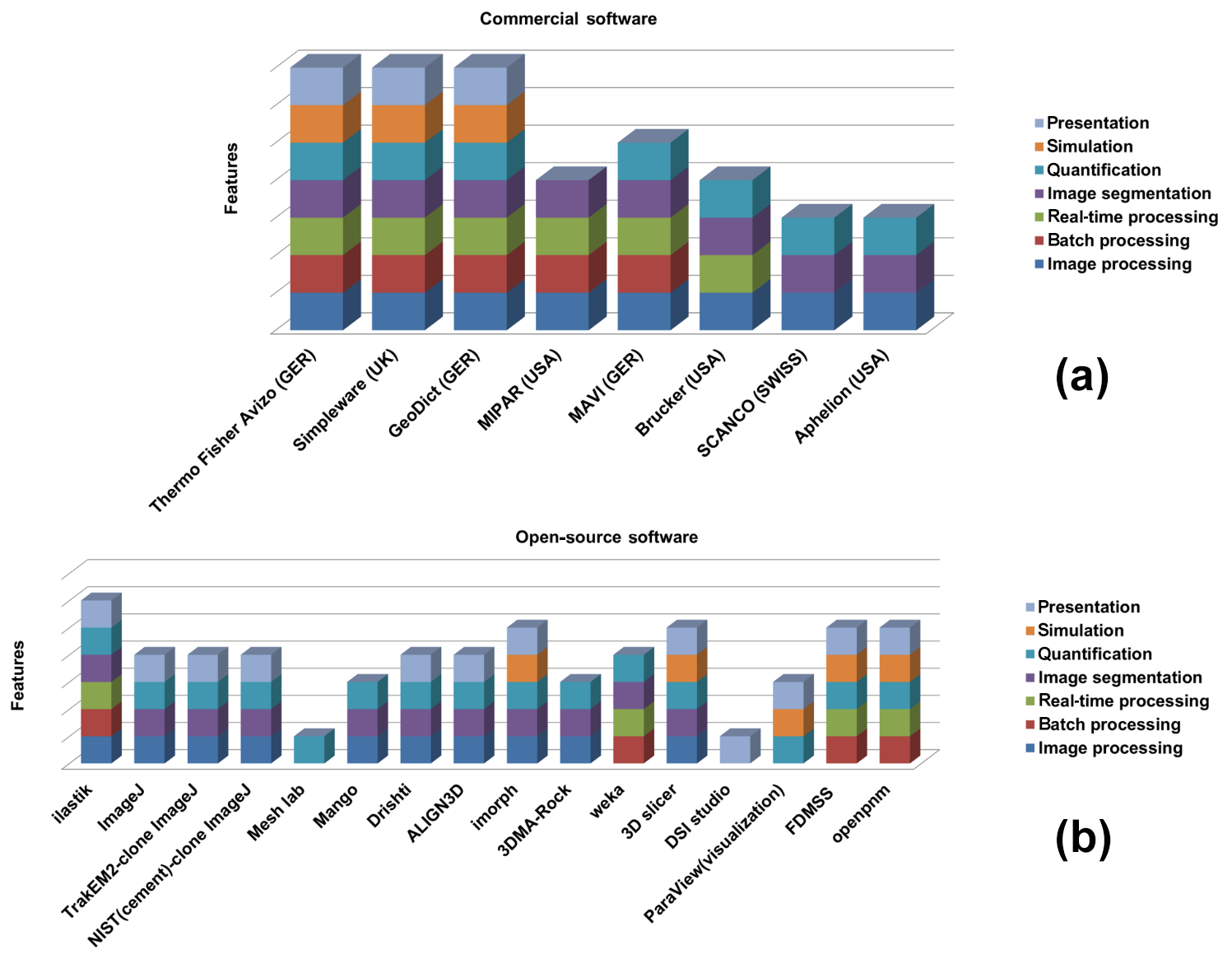
Figure 1Market survey of the currently available commercial software (a) and open-source software (b) assisting in digital rock physics analysis with features as indicated in the legend.
Currently, a vast number of available commercial and open-source software packages for pore-scale analysis and modelling exist (compiled in Fig. 1), but dedicated approaches to verify the accuracy of the segmented phases are lacking. To the best of our knowledge, the current practice among researchers is to alternate between different available software tools and to synthesize the different datasets using individually aligned workflows. Porosity and, in particular, permeability can vary dramatically with small changes in segmentation, as significant features on the pore scale get lost when thresholding greyscale tomography images to binary images, even if using the most advanced data acquiring techniques like synchrotron tomography (Leu et al., 2014). Our new CobWeb 1.0 visualization and image analysis toolkit addresses some of the challenges of selecting representative elementary volume (REV) for X-ray computed tomography (XCT) datasets reported earlier by several researchers (Zhang et al., 2000; Gitman et al., 2006; Razavi et al., 2007; Al-Raoush and Papadopoulos, 2010; Costanza-Robinson et al., 2011; Leu et al., 2014). The software is built on scientific studies which have been peer-reviewed and accepted in the scientific community (Chauhan et al., 2016a, b). The spinoff for these studies was not the lack of accuracy provided by manual segmentation schemes but the subjective assessment and non-comparability caused by the individual human assessor. Therefore, automated segmentation schemes offer speed, accuracy and possibility to intercompare results, enhancing traceability and reproducibility in the evaluation process. To our knowledge, none of the XCT software used in rock science community relies explicitly on machine learning to perform segmentation, which makes the software unique.
Despite many review articles and scientific publication highlighting potential of machine learning and deep learning (Iassonov et al., 2009; Cnudde and Boone, 2013; Schlüter et al., 2014), software libraries or toolboxes are seldom made available. Thus, with CobWeb, we started to fill this gap for the first time. Despite its limited volume-rendering capabilities, it is a useful tool, and the current version of the software can be applied in scientific and industrial studies. CobWeb provides an appropriate test platform where new segmentation and filtration schemes can be tested and used as a complementary tool to the simulation software, GeoDict and Volume Graphics. The simulation software (GeoDict and Volume Graphics) has benchmarked solvers for performing flow, diffusion, dispersion, advection-type simulation, but their accuracy relies heavily on the finely segmented datasets. This software is based on a machine learning approach with great potential for segmentation analysis, as introduced previously (Chauhan et al., 2016a, b). Further, this software tool package was developed on a MATLAB® workbench and can be used as a Windows stand-alone executable (.exe) file or as a MATLAB® plugin. The dataset for the gas hydrate (GH) sediment geomaterials was acquired using monochromatic synchrotron X-ray, unhampered by beam hardening; Sell et al. (2016) highlighted problems with edge enhancement artefact and recommended image morphological strategies to tackle this challenge. In this paper, we therefore also describe a strategy to eliminate ED artefacts using the same dataset but applying the new machine learning approach.
2.1 Image pre-processing
Image pre-processing is one of the essential and precautionary steps before image segmentation (Iassonov et al., 2009; Schlüter et al., 2014). Image enhancement filtering techniques help to reduce artefacts such as blur, background intensity and contrast variation, whereas denoise filters such as the median filter, non-local means filter and anisotropic diffusion filter can assist in lowering the phase misclassification and improving the convergence rate of automatic segmentation schemes. CobWeb 1.0 is equipped with image enhancement and denoise filters, namely imsharpen, non-local-means, anisotropic diffusion and fspecial, which are commonly used in the XCT image analysis community.
2.1.1 The imsharpen image enhancement
Despite being at the instrument level, different measures can be taken to improve the resolution of the X-ray volumetric data; the contrast in the XCT images depends particularly on the composition and corresponding densities (optical depth) of the test sample. Therefore, it is somewhat difficult to enhance contrast at the experimental setup or at the X-ray system design control stage. Thus, the contrast needs to be enhanced or adjusted after the volumetric image has been generated. For this purpose, image sharpening can be used. Image sharpening is a sort of contrast enhancement. The contrast enhancements generally take place at the contours, where high and low greyscale pixel value intensities meet (Parker, 2010).
2.1.2 Anisotropic diffusion image filtering
For intuition purposes, an anisotropic diffusion (AD) filter can be thought as a (Gaussian) blur filter. AD blurs the image, where it carefully smooths the textures in the image by preserving its edges (Kaestner et al., 2008; Porter et al., 2010; Schlüter et al., 2014). To achieve the smoothing along with edge preservation, the AD filter performs an iteration to solve non-linear partial differential equations (PDEs) of diffusion:
where I is the image, t is the time of evolution, and c is the flux which controls the rate of diffusion at any point in the image.
Perona and Malik (1990) introduce a flux function c to follow an image gradient and stop or restrain the diffusion when it reaches the region boundaries (edge preservation). This is given by
Here, the parameter κ is a tuning parameter that determines if the given edge to be considered as a boundary or not. A large value of κ leads to an isotropic solution, and the edges are removed. For our investigations, the parameter κ (threshold stop) was fixed to the value 22 968, which is the edge preservation limit between quartz grain and hydrate phase. The desired denoising (blurring/smoothing) was achieved within five iteration steps.
2.1.3 Non-local means image filtering
The non-local means (NLM) filter is based on the assumption that the image contains an extensive amount of self-similarity (Buades et al., 2005; Shreyamsha Kumar, 2013). Based on this assumption, Buades et al. (2005) extended the linear neighbourhood SUSAN filter (Smith and Brady, 1997) with non-local class. Thus, through the non-local class, the spatial search for similar pixel values is not restricted to a constrained neighbourhood pixel but the whole image is part of the search for similar pixel values. This is given by the following equation:
where NL(i) is the estimated non-local intensity of the pixel i, I is the image, and w(i,j) is the weight (or average value) applied to noisy image v(j) to obtain and restore the pixel i.
However, for a practical and computational reason, the search is performed within a search window or neighbourhood patches, and w(i,j) evaluates similarity in pixel intensities between local neighbourhood patches. Here, the weight w(i,j) is calculated as
where Z(i) is a normalization constant:
where v(Ni),v(Nj) are the local neighbourhood patches.
The similarity is fulfilled as the Euclidean distance between the local neighbourhood patches exponentially decreases. σ>0 is the standard deviation. In Eqs. (5) and (6), the distance function is pointwise multiplied (convolved) with σ to ensure a fair contribution of pixel values to the weighted function.
2.1.4 The fspecial image filtering
The fspecial filter helps in creating 2-D high-pass and low-pass filters. High-pass filters are used for sharpening and edge detection, whereas low-pass filters are used for smoothing the image quality. Frequently used high-pass filters are Laplacian and Sobel masks (kernel), and the most often used low-pass filter is the Gaussian smoothing mask (mask). However, in the current version of CobWeb, fspecial is implemented as an averaging filter. The filter is directly applied on the 2-D slices without any convolution with the filter kernel.
2.2 Image segmentation
A digital image comprises pixels of colour or greyscale intensities. Image segmentation is partitioning or classifying the pixel intensities into disjoint regions that are homogenous with respect to some characteristics (Bishop, 2006). There are continuous research efforts done in various international groups to improve and develop image segmentation approaches (Mjolsness and DeCoste, 2001). In particular, the most popular and relevant image segmentation approaches for analysing X-ray tomographic rock images are presented in the review studies done by Iassonov et al. (2009) and Schlüter et al. (2014). We use machine learning techniques for image segmentation and have implemented algorithms such as k means, fuzzy c means (unsupervised), least-square support vector machine (LSSVM) (supervised), bragging and boosting (ensemble classifiers) for automatic segmentation Chauhan et al. (2016a, b) and references therein. The performance of these machine learning technique can be assessed by matrices such as entropy, receiver operational characteristics (ROCs) and 10-fold cross validation (Chauhan et al., 2016b). Below, all the above-mentioned algorithms are described in brief.
2.2.1 Unsupervised machine learning techniques
The k-means algorithm is one of the simplest, yet robust, unsupervised machine learning (ML) algorithms commonly used in partitioning data (MacQueen, 1967; Jain, 2010; Chauhan et al., 2016b). Through an iterative approach, the k-means algorithm computes the Euclidean distance between the data points (pixel value) to its nearest centroid (cluster). The iteration converges when the objective function, i.e. the mean square root error of Euclidean distance, reaches the minimum. This is when each of the pixels in the dataset is assigned to its nearest centroid (cluster). However, the k-means algorithm has the tendency to converge at local minima without reaching the global minimum of the objective function. Therefore, it is recommended to repeatedly run the algorithm to increase the likelihood that the global minimum of the objective function will be identified. The performance of the k-means algorithm is influenced predominantly by the choice of the cluster centres (Chauhan et al., 2016b).
The fuzzy c-means (FCM) clustering procedure involves minimizing the objective function (Dunn, 1973):
where , ck is the kth fuzzy cluster centre, m is the fuzziness parameter, and m⋅uij is the membership function.
Unlike k means, FCM performs a sort of soft clustering; in the FCM iterative scheme, each data point can be a member of multiple clusters (Dunn, 1973; Bezdek et al., 1987; Jain et al., 1999; Jain, 2010). This notion of fuzzy clustering can be controlled by using a membership function (Zadeh, 1965). The membership value is in the range [0,1], and by selecting different membership values, the distance function can be regularized “loosely” or “tightly”, and certain material phases with low volume fraction can be conserved from being clustered in adjoining cluster boundaries. However, it is essential to test different combinations of membership values with several centroid centres (segmentation classes) to obtain reliable results.
2.2.2 Supervised machine learning techniques
Similar to unsupervised techniques, the objective of the supervised machine learning technique is to separate data. The advantage supervised technique offers compared to unsupervised technique is that it is effective in separating non-linear separable data (Haykin, 1995; Bishop, 2006). Datasets can be linearly separable if the points in the dataset can be partitioned into two classes using a threshold function (threshold should not be a piecewise discontinuous function). Loosely speaking, the threshold function fits a line to produce the partition. On the contrary, if we try to fit a threshold function to a substantially overlapped dataset, this usually leads to wrong partitioning (Bishop, 2006; Haykin, 1995). Therefore, a dataset which has values very close to each other is regarded as a linearly inseparable dataset (Bishop, 2006). In a supervised technique, the prediction is made by a model. The model is a mathematical function which fits a line or a plane between linearly or non-linearly separable data to classify them into different categories. The model's ability or intuition regarding where to place the line or plane between the datasets to clearly separate (classify) them is based on its (model) a priori knowledge of the dataset – this a priori knowledge is called the training dataset. Therefore, unlike the unsupervised technique, the supervised model needs to be trained on a subset of the dataset. The training dataset is the only “window” through which the model knows some pattern about the linear or non-linear separable dataset. How well the model has acquired the knowledge of the training dataset determines its success in prediction. If it has learned the training data accurately, it picks up noise along with the pattern and loses its generalization ability, thus failing when introduced to an (unknown) separable dataset. On the contrary, there could be failure in prediction caused due to inadequate training information provided to the model, or the selected model could be incapable of learning the information provided in the training dataset. Therefore, to manage a good tradeoff, cross-validation techniques are used to monitor the learning rates of the model (Haykin, 1995).
Support vector machine (SVM) (Haykin, 1995) and its modified version (LSSVM) are one such category of the supervised ML technique (Suykens and Vandewalle, 1999) and use the principles mentioned above. The plane separating the data is termed a hyperplane. The hyperplane has a boundary around it, which is called the margin, and the data points that lie closest to or on the margin are called the support vectors. The width of the margin governs the tradeoff, i.e. if the model is overfitted or underfitted to the training dataset, and can be verified through cross-validation techniques. If the width of the margin is two narrow (high learning rate), the model is overfitted (high variance) to the training dataset and will lose it generalization capability and may not separate the linear or non-linear separable (unknown) data accurately. If the width of the margin is too wide (very low learning rate), the model is underfitted (high bias) to the training dataset and will fail. An optimal learning model has just the appropriate width to maintain the generalization and also learn the patterns in the dataset.
If the training dataset is non-linear and inseparable in a 2-D coordinate system, it is useful to project the dataset in a 3-D coordinate system; thus, by doing so, the added dimension (3-D) helps to visualize the data and find a place to fit a hyperplane to separate them (Cover, 1965). So, SVM and LSSVM use the principle of cover theorem (Cover, 1965) to project the data into a higher dimension to make them linearly separable and transform them back to the original coordinate system (Suykens and Vandewalle, 1999). Hence, what type of projection is to be performed by the SVM or LSSVM is done by choosing the appropriate kernel function (van Gestel et al., 2004). This gives them the capability to attain the knowledge of the data and also preserve the generalization behaviour of the model or the classifier. In the original or the 2-D coordinate system, the hyperplane is no longer a line but a convex-shaped curve which has clearly separated the data and suitable margins to the support vectors. Here, 3-D implies a 2+1 dimensional space which consists of two spatial dimensions that correspond to the coordination of the pixels' position in the image and a third dimension that corresponds to that of the greyscales that evolve as a result of the LSSVM machine learning.
2.2.3 Ensemble classifier technique
As the name implies, ensemble classifier is an approach where the decision of several simple models is considered to improve the prediction performance. The idea behind using ensemble methods emulates from a typical human approach of exploring several options before making a decision. The ensemble technique is faster compared to supervised techniques. Basically, the evaluation of the decisions predicted by the simple models can be either done sequentially (bragging or boosting) or in parallel (random forest). Our toolbox used the sequential approach with a variation of bragging and boosting for classification. These bragging and boosting evaluations used tree learners (Seiffert et al., 2008; Breiman, 1996), inherited from the MATLAB® libraries.
The main differences between bragging and boosting are as follows. Bragging generates a set of simple models: first, it trains these models with the random sample and evaluates the classification performance of each model using the test subset of data. In the second step, only those models whose classification performance was low are retrained. The final predictive performance rate of the bragging classifier is an average of individual model performance. This approach minimizes the variance in the prediction, meaning if several bragging classifiers are generated from the same sample of data, their prediction capability, when exposed to the unknown dataset, will not differ much. The main difference between boosting and bragging is that bragging retrains selected models (high misclassification rate) with the complete training dataset until their respective accuracy increases, whereas in boosting, the size of the data which have been misclassified increases in ratio to the data which have been accurately classified – and thereafter all the models are retrained sequentially. The predictive performance is calculated the same way as in bragging by averaging the predictive performance rate of the individual models. This approach of boosting minimizes the bias in the prediction.
2.3 Performance
It is necessary to monitor the performance of an ML model. This ensures that the trained model does not overfit or underfit with the training dataset. The main reason for overfitting and underfitting of the model with the training dataset is directly proportional to the complexity of the ML models. However, the consequence is that an overfitted trained ML model will capture noise along with the information pattern from the training dataset and will lose its ability to generalize, hence leading to inaccurate classification when exposed to the unknown dataset, as it has high variance toward the training dataset. On the opposite side, when the ML model is underfitted with the training dataset, it is unable to learn or capture the essence of the training dataset; this can happen either due to a choice of a simple type model (e.g. linear instead of quadratic) or very little data to build a reliable model. As a consequence, the ML fails to predict as it has low variance towards the training dataset (Dietterich, 1998). So, the performance of the ML model (low variance and low bias) is an indication of how accurately it can predict. The above explanation is valid for supervised ML techniques. For unsupervised clustering techniques where there is no model available to train, the quality of the classification is judged from the classified result. One such commonly used metric is entropy (Stehl, 2002; Meilǎ, 2003; Amigó et al., 2009). In CobWeb, the performance of the ML models and the quality of the classification can be evaluated using 10-fold cross validation, entropy and ROC. The explanation of these methods is briefly described in the subsection below. For detailed information, the readers are referred to Stehl (2002), Dietterich (1998), Bradley (1997), and references therein.
2.3.1 The k-fold cross validation
The idea for k-fold cross validation was first recommended by Larson (1931). k-fold cross validation is a performance evaluation technique which checks the overfitting and underfitting of the ML model. In the k-fold technique, the training data are divided into k partitions. Thereafter, the ML model is trained with k−1 partition of data and tested on a withheld kth subset of data that has not been used for training. This process is repeated k times; through this, each data point in the training dataset gets to be tested at least once and is used for training k−1 times. As it can be seen, this approach should significantly reduce the overfitting (low variance), as most of the data are used for testing and underfitting (low bias), as almost all the data are used for training. Based on empirical evidence, k=10 is preferred.
2.3.2 Entropy
The entropy of a class reflects how the members of the k pixels are distributed within each class; the global quality measure is by averaging the entropy of all classes.
where P(i,j) is the probability of finding an item from the category i in the class j, where nj is the number of items in class j, and n is the total number of items in the distribution.
2.3.3 Receiver operational characteristics
ROC curves are one of the popular methods to cross validate ML model performance (probability of models' correct response P(C) to the predicted result) (Bradley, 1997). It has three variables:
where Tp and Tn are the true positive and true negative examples, and Cp and Cn are the total number of true positive and true negative examples obtained from the training dataset.
The accuracy is determined by calculating the area under the curve (AUC), and the simplest way to do this was by using trapezoidal approximation.
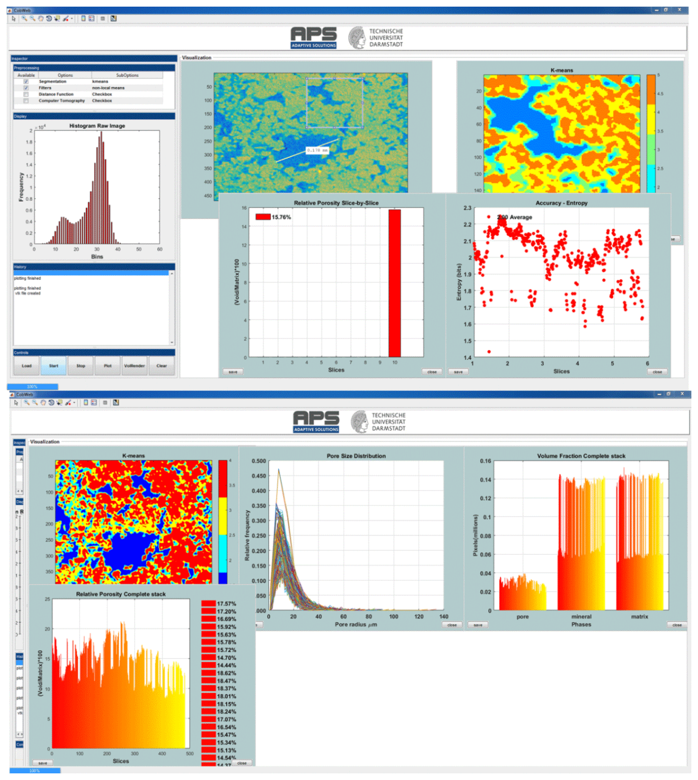
Figure 2Snapshots of the CobWeb GUI. XCT stack of Grosmont carbonate rock is shown as an example of representative elementary volume analysis. The top panel displays the XCT raw sample, the k-means segmented region of interest (ROI) and the porosity of single slice no. 10. The bottom plot shows pore size distribution of the complete REV stack, the relative porosity and volume fraction, respectively.
3.1 The graphical user interface
The first version of CobWeb offers the possibility to read and to process reconstructed XCT files in both .tiff and .raw formats. The graphical user interface (GUI) is embedded with visual inspection tools to zoom in/out, crop, colour and scale to assist in the visualization and interpretation of 2-D and 3-D stack data. Noise filters such as non-local means, anisotropic diffusion, median and contrast adjustments are implemented to increase the signal-to-noise ratio. The user has a choice of five different segmentation algorithms, namely k means, fuzzy c means (unsupervised), LSSVM (supervised), bragging and boosting (ensemble classifiers) for accurate automatic segmentation and cross validation. Relevant material properties like relative porosities, pore size distribution trends, volume fraction (3-D pore, matrix, mineral phases) can be quantified and visualized as graphical output. The data can be exported to different file formats such as Microsoft® Excel (.xlsx), MATLAB® (.mat), ParaView (.vkt) and DSI Studio (.fib). The current version is supported for Microsoft® Windows PC operating systems (Windows 7 and 10).
The main GUI window panel is divided into three main parts (Fig. 2): the tool menu strip, the inspector panel and the visualization panel. The tool strip contains menus to zoom in and out, pan, rotate, point selection, colour bar, legend bar and measurement scale functionalities. The inspector panel is divided into subpanels where the user can configure the initial process settings such as segmentation schemes (supervised, unsupervised, ensemble classifiers), filters (contrast, non-local means, anisotropic filter, fspecial) and distance functions (link distance, Manhattan distance, box distance) to assist segmentation and geometrical parameter selection for image analysis (REV, porosity, pore size distribution (PSD), volume fraction). The display subpanel records, displays the 2-D video of the XCT stack and the respective histogram. The history subpanel is a uilistbox that displays errors, processing time/status, processing instruction, files generated/exported and executed callbacks. The control subpanel is an assemblage of uibuttons to initialize the XCT data analysis process and the progress bar. The visualization panel is where the results are displayed in several resized windows, which can be moved, saved or deleted. The pan windows displayed inside the visualization module are embedded with uimenu and submenu to export, plot and calculate different variables like porosity, PSD, volume fraction, entropy, or receiver operational characteristics. To get the desired user functionalities, MATLAB® internal user-interface libraries were inadequate. Therefore, numerous specific adaptations are adopted from Yair Altman's undocumented MATLAB® website and the MATLAB® file exchange community. Specifically, the GUI layout toolbox of David Sampson is used to configure the CobWeb GUI layout; the pre-processing uitable uses the MATLAB® java component; it was designed using the uitable customization report provided by Altman (2014).
As a stand-alone module, the CobWeb GUI can be executed on different PC and HPC clusters without any license issues. The framework of CobWeb 1.0 is schematically illustrated in Fig. 3, and the direction for the arrow (left to right) represents the series in which the various functions are executed. The back-end architecture can be broadly classified into three different categories, namely the
-
control module,
-
analysis module and
-
visualization module.
3.1.1 Control module
Initially, the main figure panel is generated, followed by the tool strip dividing the main figure into different panels and subpanels as shown in Fig. 2. After that, the control buttons Load, Start, Stop, Volume Rendering and Clear are created and initialized, and the relevant information is appended in the main structure. Ideally, at this point, any button can be triggered or activated. However, upon doing so, an exception will be displayed in the history subpanel, indicating the next arbitrary steps. These are to first load the data by pressing the Load button, where the Load function checks the file properties, loads the data in .tiff and .raw formats, creates and displays 2-D video of the selected stack, saves the video file in the current folder and updates the respective variables to the main structure. The Stop button (Stop function) ends the execution. However, when the processing is inside a loop, the Stop function can break the loop only after the ith iteration. The Clear button (Clear function) deletes the data and clears all the variables in the main structure, resetting the graphical window.
3.1.2 Analysis module
The next step is data processing, triggered by pressing the Start button, which activates the Start function. The Start function concatenates the entire analysis procedure and is shown as Start() in Fig. 3. The Start() function is a densely nested loop; the bullet points and the sub-bullet points shown in Fig. 3 symbolize the outer and the inner nested loops. Initially, the data are gathered, and a sanity check is performed to evaluate if the user selected the relevant checkboxes and respective sub-options in the pre-processing uitable. If the checkboxes are not selected, an exception alert is displayed in the History panel, highlighting the error and suggesting the next possible action. The next loop is the image modification loop, where the user inputs are required. These inputs are desired classes for segmentation, the image resolution and the representative slice number. Thereafter, the representative slice is displayed on a resizable pan window inside the visualization panel shown in Fig. 2. Further, an option to select a region of interest (ROI) is proposed, which can be accepted or rejected. If accepted, a REV is cropped from the 3-D image stack based on user-defined ROI dimensions. Upon rejection, the complete 3-D stack is prepared for processing.
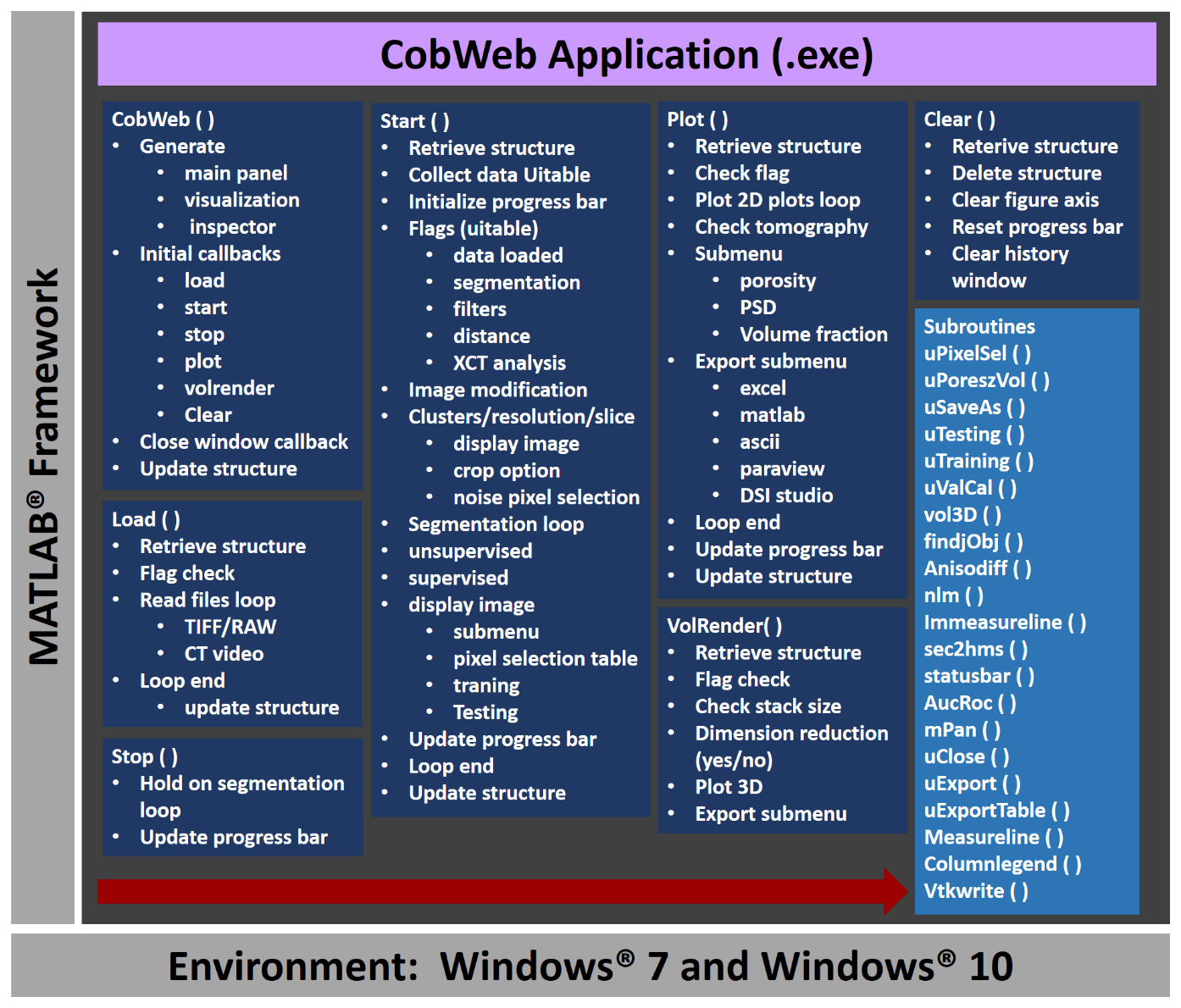
Figure 3The general workflow of the CobWeb software tool, where the arrow denotes the series in which different modules (represented in dark blue boxes) are compiled and executed. A separate file script is used to generate .dll binaries and executables.
The next step is the segmentation process; an unsupervised or supervised algorithm is initialized based on the selection made by the user in the pre-processing uitable. Hereafter, the programming logic implemented at the data access layer (also known as back-end) for unsupervised and supervised segmentation schemes is briefly explained. It is an easy one-step process in the case of unsupervised techniques; i.e. based on the options selected in the pre-processing uitable, the image is filtered and subsequently, segmented. But, for an unsupervised segmentation technique, FCM, additional user input is required. A positive decimal number x, where x is equal to is used to set the membership criteria; when pixel values of different phases (e.g. Rotliegend sandstone, Grosmont carbonate rock) are in close proximity to or subsets of each other, FCM uses the membership criteria to constrain the segmentation “loosely” or “tightly” with the purpose to segregate different phases (Chauhan et al., 2016b). In the case of supervised segmentation schemes (LSSVM, bragging and boosting), a priori information, also known as feature vector dataset or training dataset, is required to train the model(s) (Chauhan et al., 2016a, b), and consequently, the trained model is ready to classify the rest of the dataset. The following five steps accomplish this procedure:
-
First, the visualization panel displays a single 2-D slice of the REV or 3-D image stack in a resizable pan window. The embedded uimenu in the pan window offers to use the subuimenu options to feature vector selection, training and testing.
-
Second, by pressing the subuimenu option Pixel Selection, the feature vector (FV) selection performs an operation. The Pixel Selection callback function initializes the subroutine uPixelSel(), which sequentially displays a uitable in a resizable pan window. The uitable contains columns Features, X-Coordinate and Y-Coordinate, which are, for example, the pixel coordinates of the pore, matrix, minerals and noise/speaks. This is a mandatory step to build the training dataset. The user enters this information in the respective columns of the uitable.
-
In the third step, the user has to identify features, such as pores, minerals, matrix and noise/specks, in the 2-D image using zoom-in and zoom-out tools available in the toolbar. The x coordinates and y coordinates of the identified features need to be extracted using the data cursor tool, also available in the toolbar. If satisfied, the user can enter the features and the corresponding x, y coordinates in the Pixel Selection uitable.
-
In the fourth step, the data are gathered and exported for training. This is done by pressing the export button placed on the uitable pan window, which initiates the subroutine uExportTable(). The export subroutine collects a total of 36 (6×6) pixel values in the perimeter of the user-specified x, y coordinates in the uitable.
-
In the fifth step, the model is trained. This is done by using the subuimenu in the 2-D pan window. As and when the training is finished, a notification appears on the History panel. Thereafter, by pressing the testing option in the subuimenu, the complete REV or 3-D stack can be segmented.
A progress bar offers to monitor the state of the process. Further, the History window displays information related to processing time, implemented image filters and the segmentation scheme. Finally, all relevant information and the segmented data are appended to the main structure.
3.1.3 Visualization module
Once the processing is finished, the segmented data can be visualized in the 2-D format using Plot button or in a 3-D rendered stack using VolRender button. Figure 3 depicts the nested loop structure of the Plot() and VolRender() callback functions. Upon initialization, the Plot() callback accesses the main structure and plots the segmented 2-D image of the segmented slice consecutively in a resizable pan window in the visualization panel. The displayed pan window is embedded with a uimenu and corresponding subuimenu. The uimenu items and the subuimenu options are
-
geometrical parameters → porosity, pore size distribution, volume fraction;
-
performance → entropy, ROC, 10-fold cross validation;
-
export stack → ParaView, raw.
The methods used to calculate geometrical parameters and validation schemes are benchmarked in Chauhan et al. (2016a, b). Therefore, the selection of desired options initializes respective subroutines (uPoreSzVol, uCalVal, uExport) and plots the results, as shown in Fig. 2. If required, the export of these parameters (porosity, PSD, volume fraction, entropy, ROC; 10-fold cross validation) is possible to Excel, ASCII or MATLAB® for further statistical analysis. Using the Export Stack item, the export of the 3-D segmented volume to ParaView (.vtk files) or as .raw format files is feasible for the purpose of visualization or digital rock physics (DRP) analysis. The volume-rendering functionalities of CobWeb 1.0 are simple in comparison to those of ParaView or DSI Studio. The VolRender() function renders the 3-D dataset using an orthogonal plane 2-D texture mapping technique (Heckbert, 1986) and is best suited for OpenGL hardware. The user has the option to render the 3-D stack in the original resolution or at lower resolution; the lower resolution enhances the plotting speed but degrades the image quality 10-fold. Due to this, we recommend to export the 3-D stack to ParaView or DSI Studio for visualization. This concludes the description of the toolbox and functionalities section. For more information on the usage of the graphical user interface, the user manual can be consulted, which is available as supporting information.
In the following sections, the CobWeb toolbox is demonstrated by means of three showcase examples, which are briefly introduced in terms of underlying imaging settings, research question and challenges for image processing.
4.1 GH-bearing sediment
The in situ synchrotron-based tomography experiment and post-processing of synchrotron data conducted to resolve the microstructure of GH-bearing sediments are given in detail by Chaouachi et al. (2015), Falenty et al. (2015) and Sell et al. (2016). In brief, the tomographic scans were acquired with a monochromatic X-ray beam energy of 21.9 KeV at the Swiss Light Source (SLS) synchrotron facility (Paul-Scherrer-Institute, Villigen, Switzerland) using the TOMCAT beamline (Tomographic Microscope and Coherent Radiology Experiment; Stampanoni et al. 2006). Each tomogram was reconstructed from sinograms by using the gridded Fourier transformation algorithm (Marone und Stampanoni, 2012). Later, a 3-D stack of voxels (volume pixels) was generated, resulting in a voxel resolution of 0.74 and 0.38 µm at 10-fold and 20-fold optical magnification.
4.1.1 Dual filtration of GH-bearing sediment
The ED artefact is the high and low image contrast seen between the edges of the void, quartz and GH phases in the GH tomograms. It certainly aids in clear visual distinction of these phases but becomes a nuisance during the segmentation process. Several approaches to reduce ED artefact in GH tomograms and its effect on segmentation and numerical simulation have been discussed in Sell et al. (2016). Based on our experience, a combination of the NLM filter and the AD filter, implemented using Avizo (Thermo Scientific), works best in removing ED artefacts for our GH data. In short, AD was used for edge preservation and NLM for denoising. In this study, the NLM filter was set to a search window of 21, local neighbourhood of 6 and a similarity value of 0.71. The NLM filter was implemented in 3-D mode to attain desired spatial and temporal accuracy and was processed on a CPU device.
4.1.2 GH-bearing sediment dual clustering
The edge enhancement effect was significant in all the reconstructed slices of the GH dataset. The ED effect was noticeable around the quartz grains, with high and low pixel intensities adjacent to each other. The high-intensity pixel values (EDH) were very close to GH pixel values, while the low-intensity pixel values (EDL) showed a variance between noise and void phase pixel values. Therefore, immediate segmentation performed on the pre-filtered GH datasets using CobWeb 1.0 resulted in misclassification. Further parameterizing and tuning the unsupervised (k-means) and supervised (LSSVM) modules of CobWeb 1.0 specifically, distance function (i.e. functions Euclidean distance sqeuclidean, sum of absolute differences cityblock and mandist) and different permutation and combination of kernel type, bandwidth and cross-validation parameters, showed significant improvement, but the segmentation was still not optimal. The aim was to eliminate the ED features completely without altering the phase distribution between GH and the void. This prompted to develop a GH-specific workflow, as explained below. The Supplement provides the MATLAB® script for this workflow, which is comprised of five steps:
-
Step 1: filtering and REV selection. Four REVs of size 4×7003 were cropped from the raw (16-bit) data stack. These REVs were dual filtered using AD and NLM filters (see Sect. 4.1.1). Figure 5 depicts a 2-D dual-filtered image from REV1. In this study, the NLM filter was set to a search window of 21, local neighbourhood of 6 and a similarity value of 0.71. The NLM filter was implemented in 3-D mode to attain desired spatial and temporal accuracy and was processed on a CPU device.
-
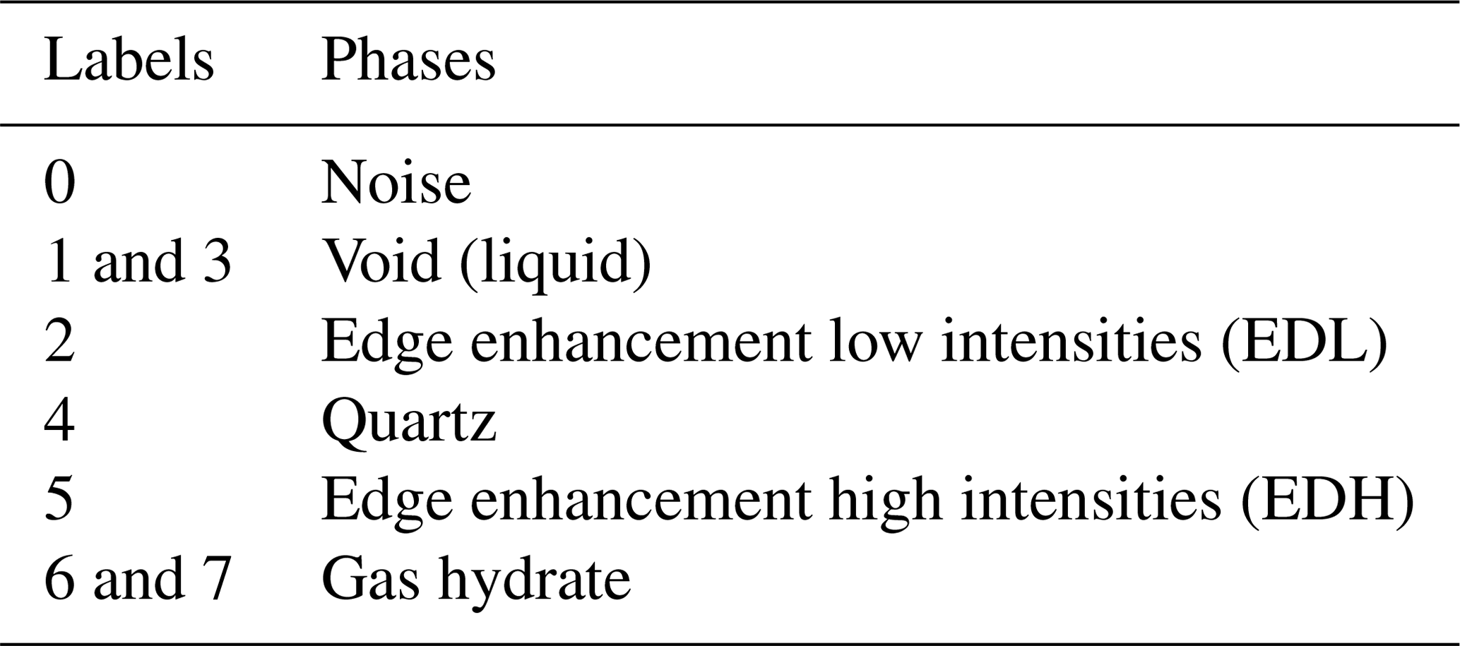
Step 2: k-means clustering. After dual filtration (step 1), it was essential to segregate the noise, edge enhancement effects and different phases into labels of various classes. This was accomplished by k-means segmentation. In order to capture all the phases accurately along with noise and ED affects, a segmentation process with up to 20 class labels was needed and performed. As a result, class 7 captured all the desired phases (noise, edge enhancement low intensities (EDL), void, quartz and edge enhancement high intensities (EDH), GH).
-
Step 3: indexing. In the next step, the purpose was to retrieve pixel values of various phases from the dual-filtered REV stacks. The indexing scheme is the following:
-
First, through visual inspection of the segmented image (step 2), different phases and their corresponding labels were identified, shown in Table 1.
-
Thereafter, pixel indices of these phases were extracted from the segmented image based on their labels.
-
Further, these indices were used as a reference mask to retrieve pixel values of the phases from the 16-bit raw REV stacks.
The obtained pixel values represent noise, void (liquid), EDL, quartz, EDH, and GH phases in the raw images. Then, the histogram distribution of the pixel values in each phase was plotted. The skewness of the histograms was investigated where the max, min, mean and standard deviation for each of the histograms were calculated. Thereafter, the max and min of the histograms were compared, and the indexing limits were adjusted, as long as there was no overlap found amidst the histogram boundaries.
-
-
Step 4: rescaling raw REV. In this step, the raw pixel values of the respective phases, i.e. void, quartz and GH, were replaced by their mean values, with an exception for EDH pixel values. The latter (EDH pixels) were replaced with the mean value of quartz. These assignments led to optimal segregation of the phase boundaries in the raw dataset and finally to the elimination of the ED effect.
-
Step 5: k-means clustering. Finally, the rescaled raw REV was segmented into three class labels using k-means segmentation to obtain the final result.
4.2 Grosmont carbonate rock
The digital rock images of the Grosmont carbonate rock were obtained from the FTP server GitHub (http://github.com/cageo/Krzikalla-2012, last access: 24 January 2020) used in the benchmark study published by Andrä et al. (2013a, b). Grosmont carbonate rock was acquired from Grosmont Formation in Alberta, Canada. The Grosmont Formation was deposited during the upper Devonian and is divided into four facies members: LG UG-1, UG-2, and UG-3 (bottom to top). The sample was taken from UG-2 facies and is mostly composed of dolomite and karst breccia (Machel and Hunter, 1994; Buschkuehle et al., 2007). Laboratory measurements of porosity and permeability reported by Andrä et al. (2013b) are around 21 % (ϕ=0.21) and κ=150–470 mD, respectively. The Grosmont carbonate dataset was measured at the high-resolution X-ray computed tomographic facility of the University of Texas with an Xradia MicroXCT-400 instruments (ZEISS, Jena, Germany). The measurement was performed using 4× objective lenses, 70 kV polychromatic X-ray beam energy and a 25 mm charge coupled device (CCD) detector. The tomographic images were reconstructed from the sinograms using proprietary software and corrected for the beam hardening effect, which is typical for lab-based polychromatic cone-beam X-ray instruments (Jovanović et al., 2013). The retrieved image volume was cropped to a dimension of 10243 with a voxel size of 2.02 µm.
4.3 Berea sandstone rock
The Berea sandstone digital rock images were part of a benchmark project published by Andrä et al. (2013a, b) and obtained from the GitHub FTP server. The Berea sandstone sample plug was acquired from Berea Sandstone™ petroleum cores (Ohio, USA). The porosity value of 20 % (ϕ=0.20) was obtained using a helium pycnometer AccuPyc™ 1330 (Micromeritics Instrument Corp., Germany) and a Pascal mercury porosimeter (Thermo Scientific™) as described in Giesche (2006). The permeability ranges between κ=200 mD and κ=500 mD, as reported by Andrä et al. (2013b). Machel and Hunter (1994) identified minerals using a polarized optical microscope and a scanning electron microscope, and reported a mineral composition of ankerite, zircon, k-feldspar, quartz, and clay in the Berea sandstone sample. The synchrotron tomographic scans of Berea sandstone were also obtained at the SLS TOMCAT beamline. The beam energy was monochromatized to 26 keV for optimal contrast, with an exposure time of 500 ms. This resulted in a 3-D tomographic stack with a dimension of 10243 voxels with a voxel size of 0.74 µm.
5.1 Data selection
The REV selection basically was a combination of visual inspection and consecutively segmenting and plotting trends in relative porosity, pore size distribution and volume fraction. This was done by loading the complete stack in the CobWeb software; during the loading process, a 2-D movie of the tomogram was displayed in the display window and saved in the root folder. Carefully monitoring the movie gives an objective evaluation of the heterogeneity of the respective XCT sample. We observed several subsample volumes at various locations (x, y) and depth (z) inside the XCT tomograms. Thereafter, based on a subjective visual consensus, different ROIs were selected, cropped and segmented, and their respective geometrical parameters were intercompared. The main indicator, however, was the porosity trend; i.e. when the regression coefficient (R2) value was close to zero, it was an indicator that its subvolume has accumulated the heterogeneity along the z axis of the sample. Therefore, based on the trend analysis approach, the subvolume dimension where the R2 value was close to zero was chosen as the suitable REV.

Figure 4The most suitable ROIs and corresponding REV dimensions of Berea sandstone and Grosmont carbonate GH-bearing sediment are shown in panels (a), (b) and (c), respectively.
In the case of Berea sandstone, four different ROIs were investigated, whereas with Grosmont carbonate rock seven different ROIs were needed to identify the best REVs. Cubical stack sizes between 3003 and 7003 slices were tested, and later it was established that a stack size around 4803 was the best suited. Through our previous scientific studies on the GH sediments (Sell et al., 2016, 2018), we were aware of the best-suited REVs and established that stack size of 7003 was an appropriate stack size. The identification of best REV for Grosmont was relatively tedious compared to Berea sandstone and GH sediment due to the low resolution and microporosity present in the Grosmont tomograms. Figure 4 shows the chosen ROIs of Berea, Grosmont and GH dataset, and Figs. 6 and 8 show the surface plot for respective REVs.
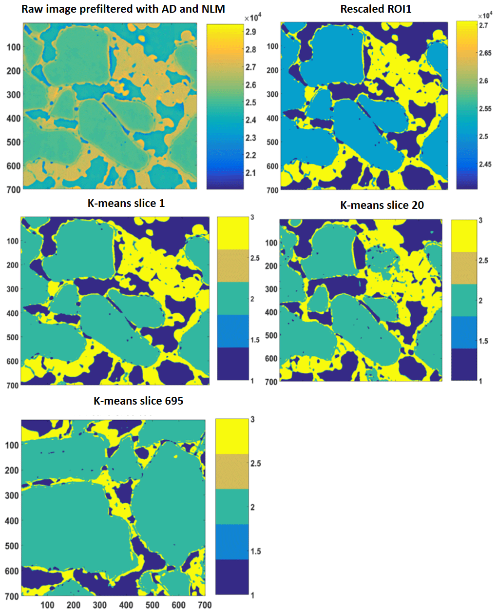
Figure 52-D slices of REV 1 are represented above. The raw image is first filtered with anisotropic diffusion filtered and later on with non-local means. Thereafter, the different phases were segregated using a segmentation and indexing approach, and the raw image(s) were rescaled such that there was no overlap or mixed phases within the raw image; an example is shown as the rescaled 2-D ROI plot. Thereafter, k-means segmentation is performed on the complete stack; 2-D images of slice 1, slice 20 and slice 695 are shown as examples.
5.2 Data processing
In the case of Berea sandstone, the 3-D reconstructed raw images (10243) had sufficient high resolution and contrast, and thus did not show any noticeable change to the filtration, whereas the XCT images (10243) of the Grosmont carbonate rock needed a non-local means filtering which yielded better visualization and performance results compared to those enhanced with the anisotropic diffusion filter. However, for the GH synchrotron dataset, the CobWeb 1.0 filters were insufficient to normalize the edge enhancement artefact. Several attempts were made to remove the edge enhancement effect using single filters and in combination with supervised techniques, but they did not yield desirable results. The edge enhancement artefact pixel values were in very close proximity to the GH sediment pixels. Therefore, pre-processing with single filters despite using appropriate settings could not normalize enhancement artefacts to a reasonable range of values. Despite tailoring a customized training dataset using a representative slice, due to a large standard deviation in the edge enhancement artefact values, GH was systematically misclassified as ED as the pixel values deviated away from the trained model. An alternative approach was to create different training datasets using several representative slices and introduce the unknown stack of data for classification in batches of 100 slices. This regularization trick for us did not represent a good norm for supervised ML classification.
Hence, through the experiments conducted in Sell et al. (2016), for us, dual filtration was one of the best approaches that we could include in the pre-processing step. This dual filtering did not remove the ED completely but rather normalized it to a reasonable range. Through the approach of rescaling and (hard) k-means segmentation (dual segmentation), we were absolutely sure that the ED artefact had been removed. This dual filtering scheme is explained in Sect. 4.1.2. It is to be noted that the NLM filter is hard-coded as 2-D in the CobWeb stand-alone version (GUI). But, by tweaking or modifying the source code, we could initially pre-process the XCT images using NLM 3-D filtration and thereafter subjected it to segmentation.
In general, our observation is that, depending on the resolution of the dataset, the fixed parameters of NLM and other filters should do a fairly good job. In the event that there still exists noise and artefacts, we recommended that the supervised techniques be used. The supervised techniques offer the possibility to select the residual noise or artefact pixel values before or after the filtration (pre-processing) through proper feature vector selection, and further train the appropriate model and performing classification. Through this, the existing noise and artefact can be isolated and segmented as separate labels. Another alternative option could be to pre-process the data with desired filter data and import the data into CobWeb for segmentation and analysis.
Another issue has to be explained in more detail in the implementation of the image segmentation. CobWeb 1.0 uses a slice-by-slice 2-D approach. It was observed that the ML techniques tend to underestimate porosity values compared to manually segmented analysis at a REV scale size > 5003. This substantial degree of uncertainty is caused due to 2-D slice-by-slice processing rather than the ML techniques. The 2-D slice-by-slice approach, passes only the spatial information (x and y coordinate direction) to the ML algorithms, and the ML algorithm ends up sorting the intensity variation in the spatial domain (local optimum). Therefore, the lack of spatial information (x-coordinate direction) restricts the degree of freedom to find a global optimum. In other words, changes due to bedding (sedimentary rock) or microporosity (carbonate rocks) in the rock texture are represented as a sudden spike or dip in porosity values, which appear as artefacts or anomalies and are often discarded. We acknowledge this issue, and correction will be implemented in the future software version; in the current workflow, it has not been accounted for (CobWeb 1.0). The 2-D slice-by-slice processing scheme is much faster compared to the 3-D approach. So, the choice of 2-D processing for this research study was made to make it affordable to compute on a desktop and laptop for near-real-time and on-site evaluation. The inaccuracies in porosities are compensated by calculation of the mean porosity of the complete stack.
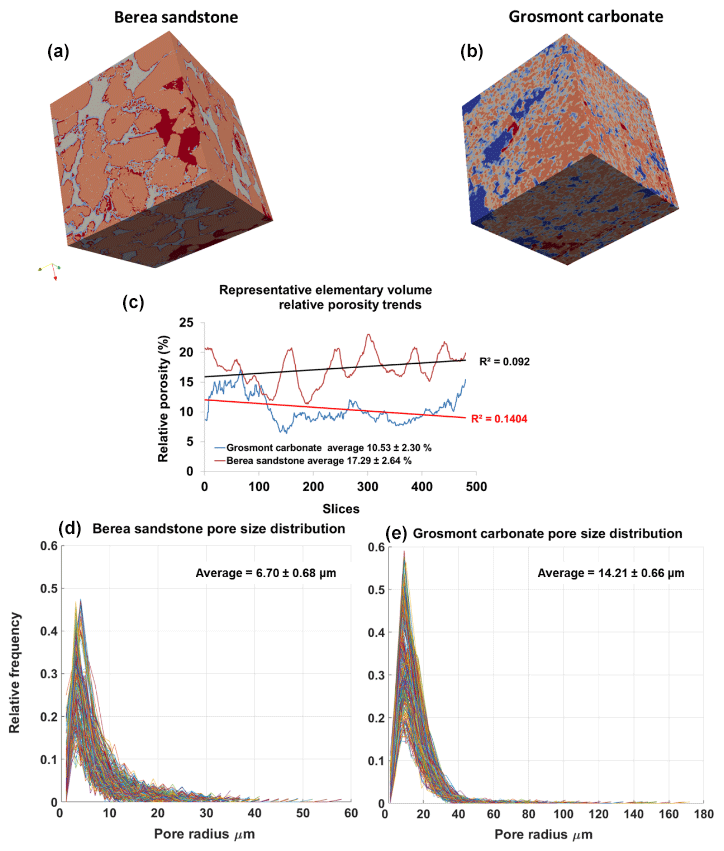
Figure 6Panels (a, b) show surface plot of REVs of Berea sandstone and Grosmont carbonate (size ) using the visualization ParaView software. Panel (c) shows the relative porosity (%) trend for Berea sandstone and Grosmont carbonate REV samples. Panels (d, e) show the pore size distribution of Berea sandstone and Grosmont carbonate. XCT images were segmented using k means. In the case of Grosmont, a non-local means filter was used.
5.3 Multiphase image segmentation
The major problem for all multiphase segmentation is that phases having intermediate greyscale values get sandwiched between two different phases. These intermediate phases sometimes represent some of the vital material properties such as connectivity. Therefore, it is vital to emphasize how ML can assist in issues related to multiphase segmentation. In a practical sense, machine learning tries to separate greyscale values into disjoint sets. The creation of these disjoint sets is commonly done in two ways:
-
The first way is by binning the greyscale values to the nearest representative values which are iteratively updated using an optimization function. This optimization function can be a simple regression or distance function (Jain et al., 1999), commonly used in unsupervised techniques.
-
The second way is by regularizing pre-trained models which store certain pattern information of the datasets such as topology features, contour intensities, pixel value, etc. (Hopfield, 1982; Haykin, 1995; Suykens and Vandewalle, 1999) or by using a voting system in a bootstrap ensemble of linear models (Breiman, 1996).
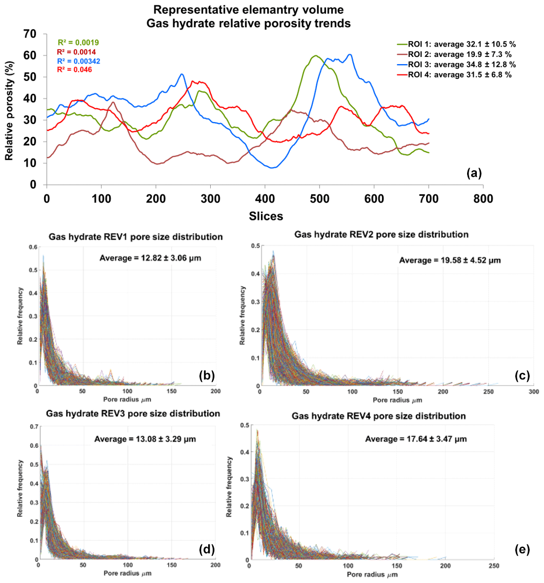
Figure 7Panel (a) shows relative porosity trend analysis of gas hydrates; panels (b–e) show the geometrical pore size distribution of the respective REVs. The analysis was performed using CobWeb 1.0.
So, in this process, the intermediate greyscale values corresponding to low volume fraction which shows multi-modal distributions are merged with greyscale values of high volume fraction to create disjoint boundaries. Through this, the intermediate phase information is misclassified and hence destroyed. One way to overcome this problem is by using supervised techniques such as LSSVM or ensemble classifiers. When constructing a training dataset (feature vector selection), careful selection of intermediate phases as a sufficiently large sample size compared to the predominant phases will preserve the intermediate phases. In addition, the likelihood that the trained model will identify them and cluster them separately is higher (Chauhan et al., 2016a). In this study, in particular, we made tests using supervised techniques (LSSVM, ensemble classifiers) and an unsupervised technique (FCM) but the results were not superior compared to k means. Therefore, we choose k means, as it was faster compared to other ML techniques. Since we have used k means for segmentation, it is necessary that we justify the performance of k means in terms of accuracy and speed. In the current research work, since we have used the unsupervised technique, it is safe to say that accuracy and speed are directly proportional to starting point (initial location) in the segmentation process. This means that the closer the starting point (initial location) is to the global minima, the faster the algorithm will converge, and the performance is even better (accuracy and speed). But, in an unsupervised technique, by default, the choice of the starting point is through random seed unless explicitly specified. So, in the case of the dual segmentation approach used for segmentation, the intuition was to capture all the material phases, including the edge enhancement artefact, speck and noise, etc., in the first step and thereafter in the second step to rescale them to the plausible phases. Hence, in the first step, the 20 clusters were initialized using random seed. And, after the rescaling processes, we were aware of the initial locations which we used as a starting point (initial location) to assist the algorithm to move towards identifying correct phases. Therefore, we could increase both the speed and accuracy of k means. In the case of Berea sandstone, the segmentation was restricted to four clusters, out of which three phases can be clearly seen. The first two phases are pores and rock; in the third phase, minerals (ankerite, zircon, k-feldspar, quartz, and clay) have been classified into a single mono-mineral phase; and the fourth phase comprises small-scale features like residual speck and noise pixels. The Grosmont carbonate sample was also segmented into four clusters comprised of pore, pore inclusions, calcite and brightness inhomogeneities of noise classified and the fourth phase.
Note that the purpose of this study was to demonstrate the capabilities of CobWeb and removal of edge enhancement segmentation through dual filtration and dual segmentation schemes. Detailed verification with LSSVM and ensemble classifiers therefore falls outside the scope of this work, and readers are referred to the previous work from Chauhan et al. (2016a) based on which CobWeb is developed. That work benchmarks different ML algorithms and quantifies their respective accuracies and performance.
5.4 Estimation of relative porosity and pore size distribution
The PSDs of the respective REVs were calculated using the CobWeb PSD module. The PSD module is based on an image processing morphological scheme (watershed transformation) suggested by Rabbani et al. (2014). As stated in Rabbani et al. (2014), the aim is to break down the monolithic void structure of rock into specific pores and throats connecting each other. Rabbani et al. (2014) used unsegmented images and performed image filtration and thereafter segmented using watershed transformation. In our case, the tomograms were already pre-processed and segmented using ML techniques. These images are converted to binary images and thereafter subjected to the image processing distance function (Rosenfeld, 1969) and the watershed algorithm (Myers et al., 2007) to extract pores and throats. City-block distance function is used to locate the void pixels (pores), and watershed with eight connected neighbourhoods was used to obtain the interconnectivity. Since the watershed algorithm is very sensitive to noise, despite the pre-processing and ML segmentation, the median filter was applied before subjecting to the watershed segmentation. Thereafter, the mean relative porosity value obtained for Berea sandstone was %, whereas for Grosmont carbonates the mean porosity value was lower ( %), as shown in Fig. 6. Particularly, in the case of Grosmont, after segmentation, the obtained porosity value ( %) is extremely low compared to the laboratory measurement (ϕ=21 %) published in Andrä et al. (2013a). The exact reason is not known but could also be partly attributed to sub-resolution pores which could not be captured due to low resolution obtained through XCT measurement. The regression coefficient value of R2=0.092 for the Berea sandstone porosity trend indicates that porosity remains constant throughout the REV sizes chosen and therefore consolidated for scale-independent heterogeneities. In the case of Grosmont carbonate rock, the chosen REV size was the best out of the five obtained, which consolidate again for scale-independent heterogeneities. The average pore size distribution thus obtained was 6.70 µm ± 0.68 µm and 14.21 µm ± 0.66 µm for Berea and Grosmont plug samples, respectively.
Similarly, the porosity and PSD of the four GH REVs were analysed using CobWeb 1.0 and are shown in Fig. 7. The low R2 values of the porosity trends justify that these GH REVs are scale independent and are an accurate representation of a large-scale system and are best suited for digital rock analysis. However, there is a high variance compared with the mean PSD values. The exact reason is unknown but may be due to the drastic increase and decrease of the quartz grains which can be seen in Fig. 5, or it could be that PSD requires much larger REV compared to that used for porosity analysis. The first and last 2-D slices of ROI 1 in Fig. 5 show either non-isotropic or isotropic distribution of quartz grains, which might have contributed to the respective high and low standard deviations seen in the porosity distribution. Figure 8 shows the surface and volume-rendered plots of REV 1 and REV 2; due to the high accuracy of segmentation, the quartz grain, brine and GH boundaries are clearly segregated, and ED effect eliminated.
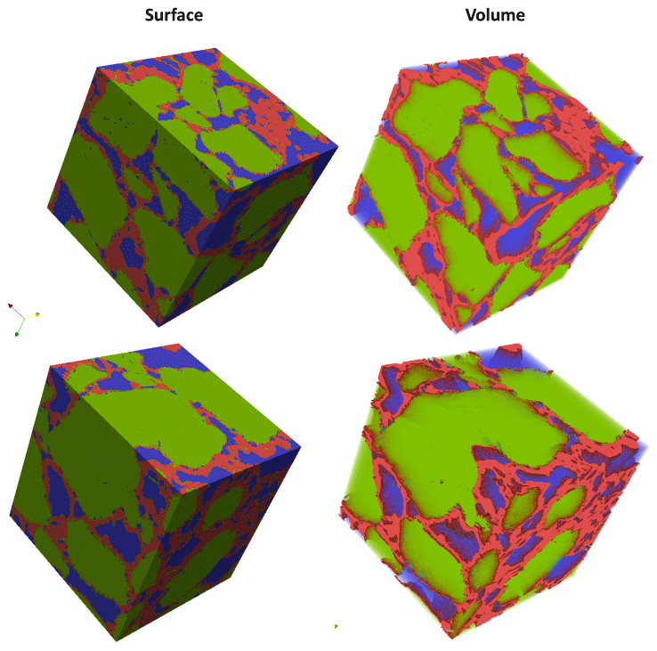
Figure 8Segmented REVs of a gas hydrate sample displayed as surface, and volume rendered and analysed using CobWeb 1.0 and exported to .vtk format using the CobWeb 1.0 ParaView plugin. The quartz grain phase is represented in green colour, gas hydrate is in red, and in blue is the void space.
This paper introduces with CobWeb 1.0, a new visualization and image analysis toolkit dedicated to representative elementary volume analysis of digital rocks. CobWeb 1.0 is developed on the MATLAB® framework and can be used as MATLAB® plugin or as a stand-alone executable. It offers robust image segmentation schemes based on ML techniques (unsupervised and supervised), where the accuracy of the segmentation schemes can be determined and results can be compared. Dedicated image processing filters such as the non-local means, anisotropic diffusion, averaging and the contrast enhancement functions help to reduce artefacts and increase the signal-to-noise ratio. The petrophysical and geometrical properties such as porosity, pore size distribution and volume fractions can be computed quickly on a single representative 2-D slice or on a complete 3-D stack. This had been validated using synchrotron datasets of the Berea sandstone (at a spatial resolution of 0.74 µm), a GH-bearing sediment (0.76 µm) and a high-resolution lab-based cone-beam tomography dataset of the Grosmont carbonate rock (2.02 µm). The gas hydrate dataset, despite its nanoscale resolution, was hampered with strong edge enhancement artefacts. A combination of the dual filtering and dual clustering approach is proposed to completely eliminate the ED effect in the gas hydrate sediments, and the code is attached in the Supplement. The REV studies performed on Berea sandstone, Grosmont carbonate rock and GH sediment using CobWeb 1.0 show relative porosity trends with very low linear regression values of 0.092, 0.1404 and 0.0527, respectively. CobWeb 1.0's ability to accurately segment data without compromising the data quality at a reasonable speed makes it a favourable tool for REV analysis.
CobWeb 1.0 is still somewhat limited regarding its volume-rendering capabilities, which will be one of the features to improve in the next version. The volume-rendering algorithms implemented in CobWeb 1.0 so far do not reach the capabilities offered by ParaView or DSI Studio, which rely on the OpenGL marching cube scheme. At present, the densely nested loop structure appears to be the best choice for systematic processing. As an outlook, vectorization and indexing approaches (bsxfun, repmat) have to be checked in detail to improve on processing speed. MATLAB® Java synchronization will be explored further to configure issues related to multi-threading and visualization (Java OpenGL). Furthermore, a module CrackNet (crack network) is planned to be implemented, which will explicitly tackle the segmentation of cracks and fissures in geomaterials using machine learning techniques and a mesh generation plugin (.stl format) for 3-D printing. Pore network extraction and skeletonization schemes such as the modified maximum ball algorithm (Arand and Hesser, 2017) and medial axis transformation (Katz and Pizer, 2003) will be considered such that the data can be exported to open-source pore network modelling packages such as the finite-difference method Stokes solver (FDMSS) for 3-D pore geometries and OpenPNM (Gerke et al., 2018; Gostick, 2017; Gostick et al., 2016).
With regards to the code availability, the MATLAB® code for removal of edge enhancement artefacts from the GH-bearing sediment is attached in the Supplement. The CobWeb executable as well as the user manual and the GH-bearing sediment XCT datasets are available to the public on the Zenodo repository https://doi.org/10.5281/zenodo.2390943 (Chauhan et al., 2019).
The CobWeb executable requires a MATLAB® runtime compiler R2017b (9.3), which can be downloaded and installed from https://de.mathworks.com/products/compiler/matlab-runtime.html (last access: 24 January 2020). The XCT dataset of Berea sandstone and Grosmont carbonate rock can be obtained from the GitHub FTP server (http://github.com/cageo/Krzikalla-2012, Andrä et al., 2012). The GH XCT datasets are not publicly available.
The supplement related to this article is available online at: https://doi.org/10.5194/gmd-13-315-2020-supplement.
SC conceptualized, investigated and performed the study. Further, SC implemented the machine learning workflow and graphical user interface design. Additionally, SC performed the formal analysis and developed a software code for the removal of the edge enhancement artefacts using the dual clustering approach. Further contributions of SC included data curation of the CobWeb software; writing the software manual and figures; and writing, reviewing and editing the manuscript.
KS conceptualized, investigated and performed a case study on gas hydrates. Further, she performed a study on the removal of edge enhancement artefacts and phase segmentation of methane hydrate XCTs. Also, she did a formal analysis by implementing the dual filtration approach to reduce the edge enhancement artefacts. KS participated in discussions to validate phase segmentation using the dual segmentation approach and was involved in writing, reviewing and editing the manuscript.
WR was involved in the project administration of the CobWeb activities and provided resources with respect to GUI and inputs on improving GUI functionalities.
TW was involved in funding acquisition and sponsoring the CobWeb project, under the framework of the SUGAR (Submarine Gashydrat Ressourcen) III project by the Germany Federal Ministry of Education and Research (grant no. 03SX38IH). He was involved in project administration and provided feedback on GUI functionalities.
IS was involved in the concept and funding acquisition for the CobWeb project, under the framework of the SUGAR (Submarine Gashydrat Ressourcen) III project by the Germany Federal Ministry of Education and Research (grant no. 03SX38IH). He also provided supervision, project administration, resources and periodic review to improve GUI functionalities.
The authors declare that they have no conflict of interest.
We thank Heiko Andrä and his team at Fraunhofer ITWM, Kaiserslautern, Germany, for providing us with the synchrotron tomography benchmark dataset of the Berea sandstone. We also thank Michael Kersten, Frieder Enzmann and his group at the Institute for Geoscience, Johannes-Gutenberg Universität Mainz, for providing high-resolution gas hydrate synchrotron data. The acquisition of the GH synchrotron data was funded by the German Science Foundation (DFG grants Ke 508/20 and Ku 920/18). This study was funded within the framework of the SUGAR (Submarine Gashydrat Ressourcen) III project by the Germany Federal Ministry of Education and Research (BMBF grant 03SX38IH). The sole responsibility of the paper lies with the authors.
We thank Kirill Gerke, two anonymous reviewers and the editor, Thomas Poulet, for their valuable comments and suggestions which significantly improved the manuscript.
This research has been supported by the BMBF (grant no. 03SX38IH).
This paper was edited by Thomas Poulet and reviewed by Kirill Gerke and two anonymous referees.
Al-Raoush, R. and Papadopoulos, A.: Representative elementary volume analysis of porous media using X-ray computed tomography, Powder Technol., 200, 69–77, https://doi.org/10.1016/j.powtec.2010.02.011, 2010.
Altman, Y.: Accelerating MATLAB Performance, CRC Press, 2014.
Amigó, E., Gonzalo, J., Artiles, J., and Verdejo, F.: A comparisonof extrinsic clustering evaluation metrics based on formal con-straints, Inform. Retrieval, 12, 461–486, 2009.
Andrä, H., Combaret, N., Dvorkin, J., Glatt, E., Han, J., Kabel, M., Keehm, Y., Krzikalla, F., Lee, M., Madonna, C., Marsh, M., Mukerji, T., Saenger, E. H., Sain, R., Saxena, N., Ricker, S., Wiegmann, A., and Zhan, X.: Digital rock physics benchmarks, available at: https://github.com/fkrzikalla/drp-benchmarks (last access: 24 January 2020), 2012.
Andrä, H., Combaret, N., Dvorkin, J., Glatt, E., Han, J., Kabel, M., Keehm, Y., Krzikalla, F., Lee, M., Madonna, C., Marsh, M., Mukerji, T., Saenger, E. H., Sain, R., Saxena, N., Ricker, S., Wiegmann, A., and Zhan, X.: Digital rock physics benchmarks – Part I: Imaging and segmentation, Comput. Geosci., 50, 25–32, https://doi.org/10.1016/j.cageo.2012.09.005, 2013a.
Andrä, H., Combaret, N., Dvorkin, J., Glatt, E., Han, J., Kabel, M., Keehm, Y., Krzikalla, F., Lee, M., Madonna, C., Marsh, M., Mukerji, T., Saenger, E. H., Sain, R., Saxena, N., Ricker, S., Wiegmann, A., and Zhan, X.: Digital rock physics benchmarks – Part II: Computing effective properties, Comput. Geosci., 50, 33–43, https://doi.org/10.1016/j.cageo.2012.09.008, 2013b.
Arand, F. and Hesser, J.: Accurate and efficient maximal ball algorithm for pore network extraction, Comput. Geosci., 101, 28–37, https://doi.org/10.1016/j.cageo.2017.01.004, 2017.
Bezdek, J. C., Hathaway, R. J., Sabin, M. J., and Tucker, W. T.: Convergence Theory For Fuzzy C-Means: Counterexamples And Repairs, IEEE T. Syst. Man. Cyb., 17, 873–877, 1987.
Bishop, C. M.: Pattern Recognition and Machine Learning (Information Science and Statistics), Springer-Verlag, Berlin, Heidelberg, 2006.
Bradley, A. P.: The use of the area under the ROC curve in the evaluation of machine learning algorithms, Pattern Recogn., 30, 1145–1159, https://doi.org/10.1016/S0031-3203(96)00142-2, 1997.
Breiman, L.: Bagging predictors, Mach. Learn., 24, 123–140, https://doi.org/10.1007/BF00058655, 1996.
Buades, A., Coll, B., and Morel, J. M.: A non-local algorithm for image denoising, IEEE Comput. Soc. Conf., San Diego, CA, USA, USA, 20–25 June 2005.
Buschkuehle, B. E., Hein, F. J., and Grobe, M.: An Overview of the Geology of the Upper Devonian Grosmont Carbonate Bitumen Deposit, Northern Alberta, Canada, Nat. Resour. Res., 16, 3–15, https://doi.org/10.1007/s11053-007-9032-y, 2007.
Chaouachi, M., Falenty, A., Sell, K., Enzmann, F., Kersten, M., Haberthür, D., and Kuhs, W.: Microstructural evolution of gas hydrates insedimentary matrices observed with synchrotron X-ray computed tomographic microscopy,Geochem. Geophys. Geosyst., 16, 1711–1722, https://doi.org/10.1002/2015GC005811, 2015.
Chauhan, S., Rühaak, W., Anbergen, H., Kabdenov, A., Freise, M., Wille, T., and Sass, I.: Phase segmentation of X-ray computer tomography rock images using machine learning techniques: an accuracy and performance study, Solid Earth, 7, 1125–1139, https://doi.org/10.5194/se-7-1125-2016, 2016a.
Chauhan, S., Rühaak, W., Khan, F., Enzmann, F., Mielke, P., Kersten, M., and Sass, I.: Processing of rock core microtomography images: Using seven different machine learning algorithms, Comput. Geosci., 86, 120–128, https://doi.org/10.1016/j.cageo.2015.10.013, 2016b.
Chauhan, S., Sell, K., Enzmann, F., Rühaak, W., Wille, T., Sass, I., and Kersten, M.: CobWeb 1.0: Machine Learning Tool Box for Tomographic Imaging, Zenodo, https://doi.org/10.5281/zenodo.2390943, 2018.
Cnudde, V. and Boone, M. N.: High-resolution X-ray computed tomography in geosciences: A review of the current technology and applications, Earth-Sci. Rev., 123, 1–17, https://doi.org/10.1016/j.earscirev.2013.04.003, 2013.
Costanza-Robinson, M. S., Estabrook, B. D., and Fouhey, D. F.: Representative elementary volume estimation for porosity, moisture saturation, and air-water interfacial areas in unsaturated porous media: Data quality implications, Water Resour. Res., 47, W07513, https://doi.org/10.1029/2010WR009655, 2011.
Cover, T. M. : Geometrical and Statistical Properties of Systems of Linear Inequalities with Applications in Pattern Recognition, IEEE Trans. Electron., EC-14, 326–334, https://doi.org/10.1109/PGEC.1965.264137, 1965.
Dietterich, T. G.: Approximate Statistical Tests for Comparing Supervised Classification Learning Algorithms, Neural Comput., 10, 1895–1923, https://doi.org/10.1162/089976698300017197, 1998.
Dunn, J. C.: A Fuzzy Relative of the ISODATA Process and Its Use in Detecting Compact Well-Separated Clusters, J. Cybernetics, 3, 32–57, https://doi.org/10.1080/01969727308546046, 1973.
Falenty, A., Chaouachi, M., Neher, S. H., Sell, K., Schwarz, J.-O., Wolf, M., Enzmann, F., Kersten, M., Haberthur, D., and Kuhs, W. F.: Stop-and-go in situ tomography of dynamic processes – gas hydrate formation in sedimentary matrices, Acta Cryst. A, 71, s154, 2015.
Gerke, K. M., Vasilyev, R. V., Khirevich, S., Collins, D., Karsanina, M. V., Sizonenko, T. O., Korost, D. V., Lamontagne, S., and Mallants, D.: Finite-difference method Stokes solver (FDMSS) for 3D pore geometries: Software development, validation and case studies, Comput. Geosci., 114, 41–58, https://doi.org/10.1016/j.cageo.2018.01.005, 2018.
Giesche, H.: Mercury porosimetry: a general (practical) overview, Part. Part. Syst. Charact., 23, 9–19, https://doi.org/10.1002/ppsc.200601009, 2006
Gitman, I. M., Gitman, M. B., and Askes, H.: Quantification of stochastically stable representative volumes for random heterogeneous materials, Arch. Appl. Mech., 75, 79–92, https://doi.org/10.1007/s00419-005-0411-8, 2006.
Gostick, J. T.: Versatile and efficient pore network extraction method using marker-based watershed segmentation, Phys. Rev. E, 96, 23307, https://doi.org/10.1103/PhysRevE.96.023307, 2017.
Gostick, J., Aghighi, M., Hinebaugh, J., Tranter, T., Hoeh, A., Michael, Day, H., Spellacy, B., Sharqawy, H., M., Bazylak, A., Burns, A., Lehnert, W., and Putz, A.: OpenPNM: A Pore Network Modeling Package, Comput. Sci. Eng., 18, 60–74, https://doi.org/10.1109/MCSE.2016.49, 2016.
Haykin, S. S.: Neural networks: A comprehensive foundation, Macmillan, New York, NY, 696 pp., 1995.
Heckbert, P. S.: Survey of Texture Mapping, IEEE Comput. Graph., 6, 56–67, https://doi.org/10.1109/MCG.1986.276672, 1986.
Hopfield, J. J.: Neural networks and physical systems with emergent collective computational abilities, P. Natl. Acad. Sci. USA, 79, 2554–2558, https://doi.org/10.1073/pnas.79.8.2554, 1982.
Iassonov, P., Gebrenegus, T., and Tuller, M.: Segmentation of X-ray computed tomography images of porous materials: A crucial step for characterization and quantitative analysis of pore structures, Water Resour. Res., 45, W09415, https://doi.org/10.1029/2009WR008087, 2009.
Jain, A. K.: Data clustering: 50 years beyond K-means, Pattern Recogn. Lett., 31, 651–666, https://doi.org/10.1016/j.patrec.2009.09.011, 2010.
Jain, A. K., Murty, M. N., and Flynn, P. J.: Data Clustering: A Review, ACM Comput. Surv., 31, 264–323, https://doi.org/10.1145/331499.331504, 1999.
Jovanović, Z., Khan, F., Enzmann, F., and Kersten, M.: Simultaneous segmentation and beam-hardening correction in computed microtomography of rock cores, Comput. Geosci., 56, 142–150, https://doi.org/10.1016/j.cageo.2013.03.015, 2013.
Kaestner, A., Lehmann, E., and Stampanoni, M.: Imaging and image processing in porous media research, Adv. Water Resour., 31, 1174–1187, https://doi.org/10.1016/j.advwatres.2008.01.022, 2008.
Katz, R. A. and Pizer, S. M.: Untangling the Blum Medial Axis Transform, Int. J. Comput. Vision, 55, 139–153, https://doi.org/10.1023/A:1026183017197, 2003.
Larson, S. C.: The shrinkage of the coefficient of multiple correlation, JPN J. Educ. Psychol., 22, 45–55, https://doi.org/10.1037/h0072400, 1931.
Leu, L., Berg, S., Enzmann, F., Armstrong, R. T., and Kersten, M.: Fast X-ray Micro-Tomography of Multiphase Flow in Berea Sandstone: A Sensitivity Study on Image Processing, Transport Porous Med., 105, 451–469, https://doi.org/10.1007/s11242-014-0378-4, 2014.
Machel, H. G. and Hunter, I. G.: Facies models for middle to late devonian Shallow-Marine carbonates, with comparisons to modern reefs: a guide for facies analysis, Facies, 30, 155–176, https://doi.org/10.1007/BF02536895, 1994.
MacQueen, J. (Ed.): Some methods for classification and analysis of multivariate observations, Fifth Berkeley Symposium on Mathematical Statistics and Probability, University of California Press, 281–297, 1967.
Marone, F. and Stampanoni, M.: Regridding reconstruction algorithm for real-time tomographic imaging, J. Synchrotron Radiat., 19, 1029–1037, 2012.
Mjolsness, E. and DeCoste, D.: Machine Learning for Science: State of the Art and Future Prospects, Science, 293, 2051–2055, https://doi.org/10.1126/science.293.5537.2051, 2001.
Myers, G. R., Mayo, S. C., Gureyev, T. E., Paganin, D. M., and Wilkins, S. W.: Polychromatic cone-beam phase-contrast tomography, Phys. Rev. A, 76, 45804, https://doi.org/10.1103/PhysRevA.76.045804, 2007.
Perona, P. and Malik, J.: Scale-space and edge detection using anisotropic diffusion, IEEE T. Pattern Anal., 12, 629–639, https://doi.org/10.1109/34.56205, 1990.
Parker, J. R.: Algorithms for Image Processing and Computer Vision, Wiley, 2010.
Porter, M. L., Wildenschild, D., Grant, G., and Gerhard, J. I.: Measurement and prediction of the relationship between capillary pressure, saturation, and interfacial area in a NAPL-water-glass bead system, Water Resour. Res., 46, W08512, https://doi.org/10.1029/2009WR007786, 2010.
Rabbani, A., Jamshidi, S., and Salehi, S.: An automated simple algorithm for realistic pore network extraction from micro-tomography images, J Petrol. Sci. Eng., 123, 164–171, https://doi.org/10.1016/j.petrol.2014.08.020, 2014.
Razavi, M., Muhunthan, B., and Al Hattamleh, O.: Representative Elementary Volume Analysis of Sands Using X-Ray Computed Tomography, Geotech. Test. J., 30, 212–219, https://doi.org/10.1520/GTJ100164, 2007.
Rosenfeld, A.: Picture Processing by Computer, ACM Comput. Surv., 1, 147–176, https://doi.org/10.1145/356551.356554, 1969.
Schlüter, S., Sheppard, A., Brown, K., and Wildenschild, D.: Image processing of multiphase images obtained via X-ray microtomography: A review, Water Resour. Res., 50, 3615–3639, https://doi.org/10.1002/2014WR015256, 2014.
Seiffert, C., Khoshgoftaar, T. M., Van Hulse, J., and Napolitano, A.: RUSBoost: Improving classification performance when training data is skewed, in: 2008 19th International Conference on Pattern Recognition, Tampa, FL, USA, 8–11 December 2008 doi:10.1109/ICPR.2008.4761297, 2008.
Sell, K., Saenger, E. H., Falenty, A., Chaouachi, M., Haberthür, D., Enzmann, F., Kuhs, W. F., and Kersten, M.: On the path to the digital rock physics of gas hydrate-bearing sediments – processing of in situ synchrotron-tomography data, Solid Earth, 7, 1243–1258, https://doi.org/10.5194/se-7-1243-2016, 2016.
Sell, K., Quintal, B., Kersten, M., and Saenger, E. H.: Squirt flow due to interfacial water films in hydrate bearing sediments, Solid Earth, 9, 699–711, https://doi.org/10.5194/se-9-699-2018, 2018.
Shreyamsha Kumar, B. K.: Image denoising based on non-local means filter and its method noise thresholding, Signal Image Video P., 7, 1211–1227, https://doi.org/10.1007/s11760-012-0389-y, 2013.
Smith, S. M. and Brady, J. M.: SUSAN—A New Approach to Low Level Image Processing, Int. J. Comput. Vis., 23, 45–78, https://doi.org/10.1023/A:1007963824710, 1997.
Strehl, A.: Relationship-based Clustering and Cluster Ensemblesfor High-dimensional Data Mining, PhD thesis, The Universityof Texas at Austin, 2002.
Meilǎ, M.: Comparing clusterings by the variation of information.Learning theory and kernel machines, Volume 2777 of the seriesLecture Notes, in: Computer Science, Springer, Berlin, Heidelberg, 173–187, https://doi.org/10.1007/978-3-540-45167-9_14, 2003.
Suykens, J. A. K. and Vandewalle, J.: Least Squares Support Vector Machine Classifiers, Neural Process. Lett., 9, 293–300, https://doi.org/10.1023/A:1018628609742, 1999.
van Gestel, T., Suykens, J. A. K., Baesens, B., Viaene, S., Vanthienen, J., Dedene, G., de Moor, B., and Vandewalle, J.: Benchmarking Least Squares Support Vector Machine Classifiers, Mach. Learn., 54, 5–32, https://doi.org/10.1023/B:MACH.0000008082.80494.e0, 2004.
Zadeh, L. A.: Fuzzy sets, Inform. Control, 8, 338–353, https://doi.org/10.1016/S0019-9958(65)90241-X, 1965.
Zhang, D., Zhang, R., Chen, S., and Soll, W. E.: Pore scale study of flow in porous media: Scale dependency, REV, and statistical REV, Geophys. Res. Lett., 27, 1195–1198, https://doi.org/10.1029/1999GL011101, 2000.