Marine biogeochemical cycling and oceanic CO₂ uptake simulated by the NUIST Earth System Model version 3 (NESM v3)

In this study, we evaluate the performance of the Nanjing University of Information Science and Technology (NUIST) Earth System Model version 3 (hereafter NESM v3) in simulating the marine biogeochemical cycle and carbon dioxide (CO₂) uptake. Compared with observations, the NESM v3 reproduces the large-scale patterns of biogeochemical fields reasonably well in the upper ocean, including nutrients, alkalinity, dissolved inorganic, chlorophyll, and net primary production. Some discrepancies between model simulations and observations are identified and the possible causes are investigated. In the upper ocean, the simulated biases in biogeochemical fields are mainly associated with shortcomings in the simulated ocean circulation. Weak upwelling in the Indian Ocean suppresses the nutrient entrainment to the upper ocean, thus reducing biological activities and resulting in an underestimation of net primary production and the chlorophyll concentration. In the Pacific and the Southern Ocean, nutrients are overestimated as a result of strong iron limitation and excessive vertical mixing. Alkalinity is also overestimated in high-latitude oceans due to excessive convective mixing. The major discrepancy in biogeochemical fields is that the model overestimates nutrients, alkalinity, and dissolved inorganic carbon in the deep North Pacific, which is caused by the excessive deep ocean remineralization. The model reasonably reproduces present-day oceanic CO₂ uptake. Model-simulated cumulative oceanic CO₂ uptake is 149 PgC between 1850 and 2016, which compares well with data-based estimates of 150±20 PgC. In the 1 % yr⁻¹ CO₂ increase (1ptCO₂) experiment, the diagnosed carbon-climate ($\mathit{\gamma }=-\mathrm{7.9}$ PgC K⁻¹) and carbon-concentration sensitivity parameters (β=0.88 PgC ppm⁻¹) in the NESM v3 are comparable with those in Coupled Model Intercomparison Project phase 5 (CMIP5) models (β: 0.69 to 0.91 PgC ppm⁻¹; γ: −2.4 to −12.1 PgC K⁻¹). The nonlinear interaction between carbon-concentration and carbon-climate sensitivity in the NESM v3 accounts for 10.3 % of the total carbon uptake, which is within the range of CMIP5 model results (3.6 %–10.6 %). Overall, the NESM v3 can be employed as a useful modeling tool to investigate large-scale interactions between the ocean carbon cycle and climate change.

1 Introduction

The global carbon cycle plays an important role in the climate system. The increase in atmospheric CO₂ is responsible for a large part of the observed increase in global mean surface temperature (Ciais et al., 2013). From 1750 to 2016, about 645±80 PgC (1 PgC =10¹⁵ g carbon) of anthropogenic carbon was emitted to the atmosphere, including 420±20 PgC from fossil fuels and industry and 225±75 PgC from land use change (Le Quéré et al., 2018). This CO₂ emission caused atmospheric CO₂ concentration to increase by 48 % from an annual mean preindustrial (PI) value of ∼277 parts per million (ppm) (Joos and Spahni, 2008) to 409.8 ppm in 2019 (Dlugokencky and Tans, 2020). As a large carbon reservoir, the global ocean contains more than 50 times the amount of carbon in the atmosphere (Denman et al., 2007) and plays a key role in anthropogenic CO₂ uptake (Ballantyne et al., 2012; Wanninkhof et al., 2013). From the year 1870 to 2016, about 25 % of anthropogenic CO₂ (about 150±20 PgC) was absorbed by the ocean (Le Quéré et al., 2018).

An increase in atmospheric CO₂ perturbs the atmospheric radiative balance and leads to climate change. Changes in atmospheric temperature, precipitation, evaporation, and wind induce changes in ocean physical properties, including temperature, salinity, and ocean circulation (Gregory et al., 2005; Pierce et al., 2012). These changes in ocean physical properties, in turn, affect the ocean carbon cycle (Sarmiento and Gruber, 2006). Friedlingstein et al. (2006) proposed that the response of the oceanic uptake of atmospheric CO₂ can be represented by the linear sum of two components: (1) carbon-concentration sensitivity, which refers to the response of oceanic CO₂ uptake to increasing atmospheric CO₂; and (2) carbon-climate sensitivity, which refers to the response of oceanic CO₂ uptake to global warming. Adopting this conceptual framework, a number of studies have analyzed the effect of increasing atmospheric CO₂ concentration and global warming on the carbon cycle in terms of the carbon-concentration and carbon-climate sensitivity parameters under different CO₂ emission and concentration scenarios (Gregory et al., 2009; Boer and Arora, 2009; Tjiputra et al., 2010; Roy et al., 2011; Arora et al., 2013; Schwinger and Tjiputra, 2018).

Given the importance of carbon cycle feedback in current and future global climate change, it is necessary to include the representation of the global carbon cycle in climate system models (Denman et al., 2007). The first and second generations of the NUIST climate system model show good skill in simulating internal climate modes and the global monsoon (Li et al., 2018; Yang and Wang, 2019; Yang et al., 2018). However, the previous generations of the NESM do not include an active ocean biogeochemical model and cannot be used to study the ocean carbon cycle (Cao et al., 2015). Recently, the third version of the NUIST Earth System Model (NESM v3) was developed as a newly registered model to the Coupled Model Intercomparison Project phase 6 (CMIP6; Cao et al., 2018; Eyring et al., 2016). The NESM v3 couples the Pelagic Interactions Scheme for Carbon and Ecosystem Studies version 2 (PISCES v2; Aumont et al., 2015) to represent the ocean biogeochemical processes.

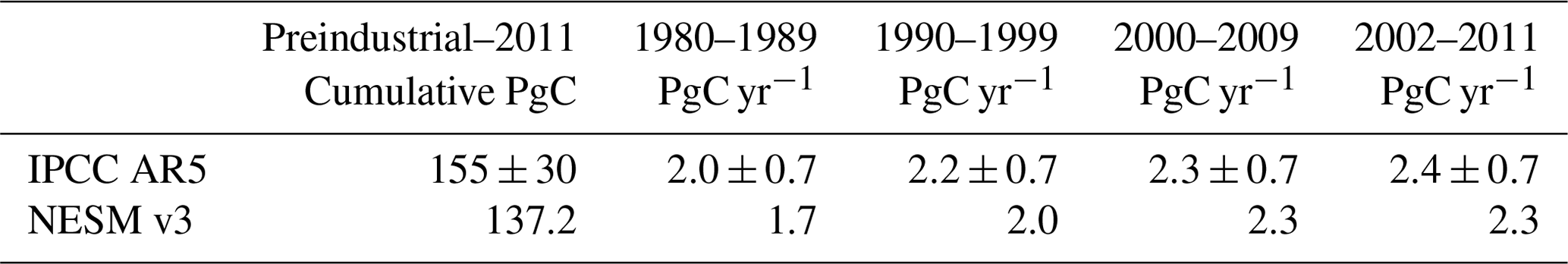
Table 1 Global ocean anthropogenic CO₂ uptake simulated by the NESM v3 during different periods compared against data-based estimates (Ciais et al., 2013). (The uncertainty ranges are given after ±, and it is noted that the preindustrial time in this study represents the year 1850, while it represents 1750 in IPCC AR5.)

The objective of this paper is to evaluate the performance of the NESM v3 in simulating marine carbon-related biogeochemical tracers and oceanic anthropogenic CO₂ uptake. As a newly developed Earth system model and a new member of the CMIP community, it is essential to evaluate the model's ability against observational data. First, we analyze the present-day distributions of macronutrients, chlorophyll, net primary production (NPP), sea–air CO₂ flux, dissolved inorganic carbon (DIC), and alkalinity against available observations and observation-based estimates. Then, we evaluate the model-simulated anthropogenic CO₂ uptake. The amount and spatial distribution of oceanic anthropogenic CO₂ uptake during the historical period and under future scenarios are compared with observations and CMIP5 model results. The carbon-concentration and carbon-climate sensitivities of oceanic CO₂ uptake diagnosed from the NESM v3 are compared with those from CMIP5 models. We also provide a Supplement that compares biogeochemical fields simulated by the NESM v3 with that by IPSL-CM5A-LR (hereafter IPSL), which shares the same marine biogeochemical component (PISCES) as used in the NESM v3.

In Sect. 2, we describe the NESM v3 with a focus on the ocean carbon cycle component, as well as the setup of model simulations. The results of model simulations are analyzed in Sect. 3. Conclusions and a discussion are presented in Sect. 4.

2 Methods

2.1 Model

2.1.1 Framework of the NESM v3

Detailed descriptions of the physical components, major improvements, and model tuning procedures of the NESM v3 are documented in Cao et al. (2018). Here we give a brief review.

The NESM v3 consists of three main model components, including European Centre Hamburg Atmospheric Model version 6.3 (ECHAM v6.3) (Stevens et al., 2012; Giorgetta et al., 2013), Nucleus for European Modeling of the Ocean version 3.4 (NEMO v3.4, revision 3814) (Madec, 2012), and Los Alamos sea ice model version 4.1 (CICE v4.1) (Hunke et al., 2010).

In this study, we use the low-resolution version of the NESM v3. The atmospheric resolution is T31L31 that has a horizontal resolution of ∼3.75^∘ latitude by 3.75^∘ longitude and 31 layers. The atmospheric model and land surface model are originally adopted from ECHAM v6.3. A detailed description is provided in Stevens et al. (2012) and Giorgetta et al. (2013). The sea ice model includes four ice layers and one snow layer with a multi-layer thermodynamic scheme (Hunke et al., 2010; Cao et al., 2018). The ocean model has the ORCA2 global ocean configuration that is a type of tripolar grid. It is based on a 2^∘ Mercator mesh and has 31 layers with the thickness of the ocean layer increasing from 10 m in the upper ocean to 500 at 5000 m of depth. A local transformation is applied in the tropics to refine the resolution to up to 0.5^∘ at the Equator. In the ocean model, the incoming solar radiation can penetrate to the upper-ocean layers as deep as 391 m, and a bio-model penetration parameterization scheme is used to calculate the vertical distribution of solar radiation (Lengaigne et al., 2009). The ocean background vertical diffusivity is modified in the NESM v3, whereby the constant value is replaced by latitude-dependent values (Jochum, 2009). The parameterization scheme of vertical diffusivity is detailed in the Supplement, with the global distribution of vertical diffusivity shown in Fig. S1. Compared to the original vertical diffusivity coefficient constant of 0.12 cm² s⁻¹, the coefficients in the tropical ocean are reduced and those in the subtropical and high-latitude oceans are enhanced. Also, the NESM v3 incorporates the parameterization of brine rejection in the ocean model, and the reference sea ice salinity is set as 4 PSU as suggested by Smith et al. (2010).

2.1.2 Ocean biogeochemical component

The NESM v3 employs the standard PISCES v2 to represent the ocean biogeochemical cycle. The PISCES model is developed from a simple nutrient–phytoplankton–zooplankton–detritus (NPZD) model (Aumont et al., 2002). It can be used for both regional and global simulations of lower trophic levels of the marine ecosystem and ocean carbon cycle (Bopp et al., 2005; Resplandy et al., 2012; Séférian et al., 2013). In the current version, there are 24 prognostic tracers in total, including dissolved inorganic and organic carbon, alkalinity, chlorophyll, and nutrients. We use the same biogeochemical parameters as those used in Aumont et al. (2015). The only exception is the advection scheme for passive tracers. Here we use the total variance dissipation (TVD) formulation instead of the Monotone upstream scheme for conservative law (MUSCL) formulation to keep the advection scheme consistent with the one used in the physical ocean model. Both the TVD and MUSCL schemes have a good performance in biogeochemical modeling. The MUSCL scheme has a better performance in resolving the small-scale processes, while TVD scheme minimizes systematic error through numerical diffusion and is a better option for coarse-resolution models (Lévy et al., 2001a).

Two different types of phytoplankton (nanophytoplankton and diatoms) and two size classes of zooplankton (mesozooplankton and microzooplankton) are presented in the model. The life cycle of phytoplankton is regulated by processes of growth, mortality, aggregation, and grazing by zooplankton (Aumont et al., 2015). The growth rate of phytoplankton is determined by temperature, photosynthetically active radiation (PAR), and availability of nutrients, including phosphate, nitrate, silicate, iron, and ammonium. The mortality rate of phytoplankton is set as a constant and is identical for nanophytoplankton and diatoms. The aggregations of nanophytoplankton, which transform dissolved organic carbon (DOC) to particular organic matter (POM), only depend on the shear rate because the main driver of aggregation is local turbulence. In the NESM v3, this shear rate is set to 1 s⁻¹ in the mixed layer and 0.01 s⁻¹ below. The same is assumed for diatoms, while the aggregations of diatoms are further enhanced by nutrient co-limitation. For all species, phosphate, nitrate, and carbon are linked by a constant Redfield ratio. In the NESM v3, the Redfield ratio of $\mathrm{C}:\mathrm{N}:\mathrm{P}$ is set to $\mathrm{122}:\mathrm{16}:\mathrm{1}$ (Takahashi et al., 1985), and the O∕C ratio is set to 1.34 (Körtzinger et al., 2001). In contrast, the Fe∕C, chlorophyll∕C, and silicon∕C ratios are prognostically simulated by the model based on the external concentrations of the limiting nutrients as in the quota approach (McCarthy, 1980; Droop, 1983; Aumont et al., 2015).

The remineralization of semi-labile DOC can occur in either oxic water or anoxic water depending on the local oxygen concentration, and their degradation rates are specified and identical for oxic respiration and denitrification. Detritus is represented by different types, including POM, calcite, iron particles, and biogenic silica. The POM is partitioned into two size classes: a smaller class (POC: 1–100 µm) and a larger class (GOC: 100–500 µm). The sinking speed of GOC (50–200 m d⁻¹) increases with depth and is much faster than that of POC (3 m d⁻¹). A fraction of phytoplankton would be turned to POM through the processes of mortality and aggregation. The fate of the mortality and aggregation of nanophytoplankton depends on the proportion of the calcifying organisms. For nanophytoplankton, it is assumed that half of the dying calcifiers are routed to the fast-sinking particles. The same is assumed for the mortality of diatoms, and 50 % of the dying diatoms are turned to POM due to the larger density of biogenic silica compared to that of organic matter. The degradation rate of POM depends on the local temperature with a Q₁₀ factor (temperature dependence ratio) of 1.9.

The geochemical boundary condition accounts for the external nutrient supply from five different sources, including atmospheric dust deposition of iron and silicon, river recharge of nutrients, dissolved carbon, alkalinity, atmospheric deposition of nitrogen, and sediment mobilization of sedimentary iron. In the NESM v3, atmospheric deposition and river recharge are prescribed, and sediment mobilization is parameterized. At the bottom of the ocean, different sediment parameterization schemes are applied to biogenic silica, POM, and particulate iron. The amount of permanently buried biogenic silica is assumed to balance the external source, and the burial efficiency of POM is determined by the organic carbon sinking rate at the bottom following the algorithm proposed by Dunne et al. (2007). All the particulate iron would be buried into the sediment once it reaches the ocean bottom. The amount of unburied calcite and biogenic silica would dissolve back into the ocean water instantaneously. In this study, the initial conditions of the biogeochemical model have been adopted from the World Ocean Atlas 2009 (WOA09; Garcia et al., 2010) and the Global Ocean Data Analysis Project (GLODAP; Key et al., 2004; Sabine et al., 2004) datasets.

Carbonate chemistry is formulated based on the Ocean Carbon-Cycle Model Intercomparison Project (OCMIP-2) protocol (more information can be accessed at http://ocmip5.ipsl.jussieu.fr/OCMIP/, last access: 7 July 2020). The quadratic wind speed formulation proposed by Wanninkhof (1992) is used to compute the air–sea exchange of carbon and oxygen.

2.2 Simulations

In total, there are eight different simulations in this study, including one fully coupled spin-up simulation for 2000 years, one PI-control run (CTRL) for 251 years, three transient runs driven by forcing conditions from historical observational data and Shared Socioeconomic Pathway scenarios (SSP5–8.5) from 1850 to 2100 (hereafter HistSSP), i.e., fully coupled HistSSP (FC-HistSSP), biogeochemically coupled HistSSP (BC-HistSSP), and radiatively coupled HistSSP (RC-HistSSP), and three idealized 1ptCO₂ runs for 140 years, i.e., FC-1ptCO₂, BC-1ptCO₂, and RC-1ptCO₂. The detailed experimental designs are as follows.

First, the NESM v3 was spun up for 2000 years with all related parameters set to preindustrial values (the year 1850), including orbital parameters, land use, aerosol, and greenhouse gas (GHG) concentration (284 ppm for CO₂, 790 ppb for CH₄, 275 ppb for N₂O). During the last 100 years of the spin-up simulation, the average globally integrated sea–air flux is 1.0 PgC yr⁻¹. The large positive sea–air flux is a result of the three-dimensional correction of nutrients and alkalinity in the PISCES model (Séférian et al., 2013). The three-dimensional correction refers to the fact that the global inventories of nutrients and alkalinity are restored toward the observations on 1 January of every year (Aumont et al., 2015). The linear drift of globally integrated sea–air flux during the last 100 years of the spin-up simulation is 0.0006 PgC yr⁻², indicating that a quasi-equilibrium state has been reached for the global ocean carbon cycle. Global mean sea surface temperature (SST) averaged over the last 100 years of the spin-up simulation is 13.1^∘C, with a linear drift of −0.0001 ^∘C yr⁻¹, and ocean mean temperature is 3.5 ^∘C, with a linear drift of 0.00016 ^∘C yr⁻¹, indicating that the dynamic ocean component has also reached a quasi-equilibrium state.

Following the protocol of the CMIP6 historical and SSP5–8.5 experiment design (Eyring et al., 2016; Jones et al., 2016), starting from the end of the spin-up simulation, the model is further integrated with time-changing external forcings, including GHGs, ozone, aerosol, land use, and solar forcing from 1850 to 2100. For the years 1850 to 2014, GHG concentrations and other forcing conditions are taken from observations, and for the years 2015 to 2100, GHG concentrations and forcing conditions follow the SSP5–8.5 scenario. Also, we conducted a 251-year (1850–2100) PI-control simulation with all forcing conditions kept at preindustrial levels. Meanwhile, to have a direct comparison with CMIP5 results, we conducted idealized 1ptCO₂ simulations, in which the atmospheric CO₂ concentration increases at a rate of 1 % yr⁻¹ starting from the end state of the spin-up simulation with other forcings remaining at the preindustrial level. These 1ptCO₂ simulations lasted for 140 years until the atmospheric CO₂ concentration had quadrupled.

Following Friedlingstein et al. (2006) and Arora et al. (2013), we performed three types of experiments (biogeochemically coupled, radiatively coupled, and fully coupled) for HistSSP and 1ptCO₂ to separate the effect of atmospheric CO₂ and CO₂-induced global warming on the ocean carbon cycle.

1. BC simulations were performed in which the code of the ocean carbon cycle sees changing atmospheric CO₂, but the code of atmospheric radiation sees a constant preindustrial concentration of CO₂. In this way, the ocean carbon cycle is only affected by changing atmospheric CO₂, but there is no direct effect of CO₂-induced warming.

2. RC simulations were performed in which the code of the ocean carbon cycle sees preindustrial atmospheric CO₂, but the code of atmospheric radiation sees changing concentrations of atmospheric CO₂. In this way, the ocean carbon cycle is only affected by CO₂-induced warming, but there is no direct effect of changing atmospheric CO₂.

3. FC simulations were performed in which both the codes of the ocean carbon cycle and atmospheric radiation see changing concentrations of atmospheric CO₂. In this way, the ocean carbon cycle is affected by changes in both atmospheric CO₂ and CO₂-induced warming.

It is noted that, in the FC-HistSSP, RC-HistSSP, and BC-HistSSP simulations, other forcings (non-CO₂ GHGs, aerosols, and land use change) still change with time for both the atmospheric and ocean models.

2.3 Evaluation data

Global ocean distribution data for nutrient concentrations, including nitrate, phosphate, and silicate, are taken from the World Ocean Atlas 2018 (WOA18; Garcia et al., 2018). Geographic distributions of DIC, alkalinity, and anthropogenic carbon are taken from the GLODAP v2 (Key et al., 2015; Lauvset et al., 2016). Both WOA18 and GLODAP v2 data have a horizontal resolution of $\mathrm{1}{}^{\circ }\times \mathrm{1}{}^{\circ }$ with 33 levels and represent the climatology in recent decades. In this study, we assume that the densities of seawater in the model and observations are the same, and then the unit of observations is converted (µmol kg⁻¹ to mmol m⁻³) by multiplying the modeled density (kg m⁻³). We compared modeled chlorophyll in recent decades with the SeaWiFS dataset (NASA Goddard Space Flight Center, 2014), GlobColour merged data (Maritorena et al., 2010), and Ocean Colour Climate Change Initiative (OCCCI) merged data (http://www.oceancolour.org/, last access: 7 July 2020). OCCCI and GlobColour incorporate the same datasets, while their uncertainty information and algorithms are not the same.

Model-simulated NPP is compared with Moderate Resolution Imaging Spectroradiometer (MODIS) estimated marine NPP based on three different algorithms, including the Standard Vertically Generalized Production Model (VGPM), Eppley-VGPM, and the Carbon-based Production Model (CbPM). The datasets can be accessed at http://www.science.oregonstate.edu/ocean.productivity/index.php (last access: 7 July 2020). In the VGPM and Eppley-VGPM, NPP is estimated as the product of chlorophyll and photosynthetic efficiencies (Behrenfeld and Falkowski, 1997a, b). Eppley-VGPM emphasizes the photo-acclimation effect at high SSTs; i.e., the growth rate is higher in high-temperature regions (Eppley, 1972; Morel, 1991). In the CbPM, NPP is estimated as the product of carbon biomass and the growth rate (Behrenfeld et al., 2005; Westberry et al., 2008). All three datasets have a horizontal resolution of $\mathrm{1}/\mathrm{12}{}^{\circ }\times \mathrm{1}/\mathrm{12}{}^{\circ }$ and cover the period from 2003 to 2014. The distribution of observed surface ocean sea–air CO₂ flux is taken from Takahashi et al. (2009), which applies to the reference year of 2000 and has a spatial resolution of 4^∘ latitude by 5^∘ longitude.

To have a direct comparison between the NESM v3 output and corresponding observations, we interpolated all modeled results and observations to a common $\mathrm{1}{}^{\circ }\times \mathrm{1}{}^{\circ }$ grid using the distance-weighted average remapping method, except for the sea–air CO₂ flux. Due to the low resolution of observational sea–air flux, we interpolated the modeled sea–air CO₂ flux to the $\mathrm{4}{}^{\circ }\times \mathrm{5}{}^{\circ }$ grid used by Takahashi et al. (2009).

2.4 Analysis method

2.4.1 Nutrient decomposition

To examine the contribution of ocean dynamics and biogeochemical processes to the mismatch between model results and observations, we decomposed phosphate to its preformed and regenerated components following the method of Weiss (1970) and Duteil et al. (2012). The regenerated phosphate is released through the remineralization processes of organic matter, and the preformed phosphate is the remaining biotically unutilized surface phosphate, which is transported into the ocean interior by ocean circulation. The regenerated and preformed phosphate is computed as

$$\begin{array}{}\text{(1)}& {\displaystyle }{P}_{\mathrm{regenerated}}=R_{P:-{\mathrm{O}}_{\mathrm{2}}}\times \mathrm{AOU},\text{(2)}& {\displaystyle }{P}_{\mathrm{preformed}}=P-P_{\mathrm{regenerated}},\end{array}$$

where AOU is the apparent oxygen utilization, which represents the biological consumption of oxygen. It is computed as the difference between oxygen saturation and simulated oxygen concentration. $R_{P:-{\mathrm{O}}_{\mathrm{2}}}$ represents the oxidation ratio of phosphate and oxygen, which is set to 1∕163 in the NESM v3. P represents the simulated phosphate concentration.

2.4.2 Nutrient limitation

In the NESM v3, the nutrient limitation coefficient (0–1) is computed from the Michaelis–Menten equation as follows:

$$\begin{array}{}\text{(3)}& \mathrm{MM}=N/(K+N),\end{array}$$

where MM is the Michaelis–Menten coefficient, N is the nutrient concentration, and K is the half-saturation coefficient, which is parameterized based on the half-saturation constant and concentrations of nutrients, phytoplankton, and diatoms (Aumont et al., 2015).

We calculated the annual mean nutrient limitation coefficient for each nutrient (phosphate, nitrate, silicate, and iron) and then considered the nutrient with the smallest limitation coefficient to be the most limiting factor. Temperature and light are assumed to be the most limiting factors when the annual mean nutrient coefficients are greater than 0.9 (Moore et al., 2013).

2.4.3 Carbon-concentration and carbon-climate sensitivity parameters

Following Arora et al. (2013), we diagnosed the carbon-climate and carbon-concentration sensitivity parameters from two types of experiments performed by a subset of CMIP5 models, i.e., BC simulations and RC simulations.

In the BC simulations, the relationship between the atmospheric CO₂ concentration and sea–air CO₂ flux can be simplified as

$$\begin{array}{}\text{(4)}& \underset{\mathrm{0}}{\overset{t}{\int }}{F}^{\prime }\mathrm{d}t\approx \mathit{\beta }\mathrm{\Delta }{C}_{\mathrm{A}}+\mathit{\gamma }\mathrm{\Delta }T,\end{array}$$

where F^′ represents oceanic carbon uptake change in the BC simulation, ΔC_A represents atmospheric CO₂ concentration change, β represents the carbon-concentration sensitivity parameter, γ represents the carbon-climate sensitivity parameter, and ΔT represents surface air temperature change in the BC simulation.

In the RC simulations in which the oceanic carbon uptake is only affected by climate change, the relationship between temperature and sea–air CO₂ flux can be simplified as

$$\begin{array}{}\text{(5)}& \underset{\mathrm{0}}{\overset{t}{\int }}{F}^{\prime }\mathrm{d}t\approx \mathit{\gamma }\mathrm{\Delta }T,\end{array}$$

where F^′ represents oceanic carbon uptake change in the RC simulation and ΔT represents surface air temperature change in the RC simulation.

3 Results

3.1 Nutrients

Nutrients play vital roles in the ocean biogeochemical cycle. A lack of nutrients would limit the growth of phytoplankton. Figure 1 compares the model-simulated annual mean spatial distributions of nutrient concentrations averaged over the top 100 m ocean with the WOA18 observations from 1985 to 2014, including phosphate (${\mathrm{PO}}_{\mathrm{4}}^{\mathrm{3}-}$), nitrate (${\mathrm{NO}}_{\mathrm{3}}^{-}$), and silicate (${\mathrm{SiO}}_{\mathrm{4}}^{\mathrm{2}-}$). The model reproduces the observed large-scale patterns of upper-ocean mean nutrients concentrations reasonably well, with pattern correlation coefficients (PCCs) larger than 0.8 and normalized standard deviations (NSDs; model simulations are normalized by stand deviations of corresponding observations) close to 1.0. The PCCs of nitrate, phosphate, and silicate between the model simulation and WOA18 are 0.93, 0.91, and 0.83, respectively, and the NSDs of nitrate, phosphate, and silicate are 1.05, 1.06, and 1.22, respectively. For both the NESM v3 simulation and observations, the largest concentrations of phosphate, nitrate, and silicate are observed in the Southern Ocean as a result of strong vertical mixing and upwelling that bring nutrient-rich deep water to the surface (Whitney, 2011). Also, the strong iron limitation that reduces the biological uptake of macronutrients is one of the main causes of the high macronutrient level in the Southern Ocean (de Baar et al., 1990). Relatively high concentrations of nutrients are also simulated in the subarctic Pacific Ocean and the mid-eastern Pacific Ocean. Relatively low concentrations of nutrients are simulated in subtropical regions. The spatial distributions of nutrients in the NESM v3, with high concentrations in the Southern Ocean and low concentrations in the subtropical Pacific, are generally consistent with both observations and CMIP5 model results (Ilyina et al., 2013; Moore et al., 2013; Séférian et al., 2013; Tjiputra et al., 2013).

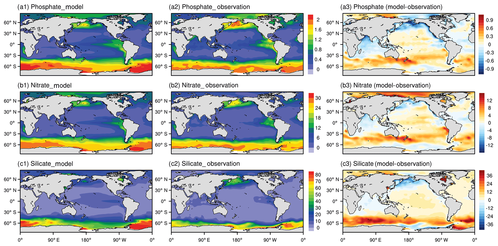
Figure 1 Annual mean (from the year 1985 to 2004) upper-ocean (averaged in the upper 100 m) distribution of phosphate (a1, a2), nitrate (b1, b2), and silicate (c1, c2) from the NESM v3 simulations (FC-HistSSP) and the WOA18 observation dataset (mmol m⁻³). The difference between the model simulation and observations is also shown (a3, b3, c3).

Some noticeable discrepancies between model simulations and observations are also found (Fig. 1a3, b3, c3). Phosphate and nitrate are overestimated in the Southern Ocean and the Pacific Ocean but underestimated in the Indian Ocean, subarctic Pacific, and tropical Atlantic. Silicate is overestimated over all of the global ocean except for the Indian Ocean and subarctic Pacific. Averaged over the global upper ocean, the model-simulated silicate concentration is about 50 % greater than that in the WOA18 observations.

Figure 2 shows the latitudinal–depth distributions of nutrients from the FC-HistSSP simulation and WOA18 observations in the Pacific, the Atlantic, and the global ocean. Nutrient distributions are reproduced well in the Atlantic by the NESM v3. The deepest penetration of relatively low-nutrient water to a 1000 m depth is simulated in the middle-latitude regions. The observed high concentration of nutrients is simulated in the Atlantic south of 45^∘ S. Also, the equatorward transport of phosphate and nitrate by Antarctic Intermediate Water near 1000 m of depth is simulated by the model. In the Pacific, the latitude–depth distributions of nutrients broadly agree with observations but with noticeable positive biases in the deep North Pacific.

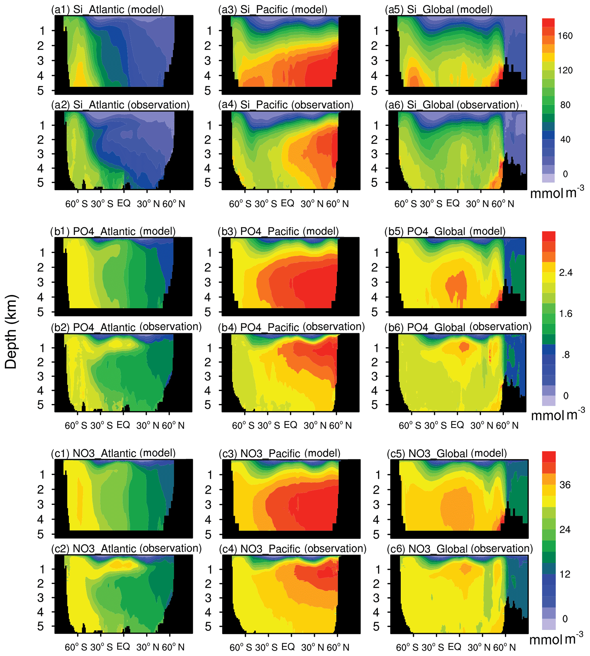
Figure 2 The latitude–depth distributions of silicate (a), phosphate (b), and nitrate (c) averaged over the years 1985 to 2014 from the NESM v3 simulation (FC-HistSSP) and the WOA18 observation dataset (mmol m⁻³). Panels (a), (b), and (c) represent silicate, phosphate, and nitrate, respectively. The labels (a1), (a2), (b1), (b2), (c1), and (c2) represent the distributions in the Pacific Ocean, labels (a3), (a4), (b3), (b4), (c3), and (c4) represent the distributions in the Atlantic Ocean, and labels (a5), (a6), (b5), (b6), (c5), and (c6) represent the distributions in the global ocean.

To further analyze the possible reasons for discrepancies in nutrient distributions between the model simulation and observations, we decomposed phosphate to its preformed and regenerated components (Weiss, 1970; Duteil et al., 2012) to compare the results with the WOA18 observations (Fig. 3). For the global ocean, Atlantic Ocean, and Pacific Ocean, the preformed phosphate diagnosed from the model accounts for 51 %, 47 %, and 57 % of the total phosphate inventory, and the result diagnosed from the WOA18 is 57 %, 55 %, and 64 %, respectively. A relatively small fraction of the preformed phosphate indicates stronger biological activities in the model. Compared to the observations, in the North Atlantic, the model underestimated the preformed phosphate, indicating that biological uptake in the upper North Atlantic is overestimated by the model. The NESM v3 overestimates the preformed phosphate above ∼500 m of depth but underestimates the preformed phosphate at the depth of 500 to 1500 m. This dipole pattern of preformed phosphate biases is associated with the overestimated vertical mixing that brings excessive nutrient-rich water from the intermediate ocean to the surface (Fig. 3a2, a4, and a6). In the deep Pacific Ocean, the preformed phosphate concentrations are between 1.3 and 1.5 mmol m⁻³ for both the model simulation and observations.

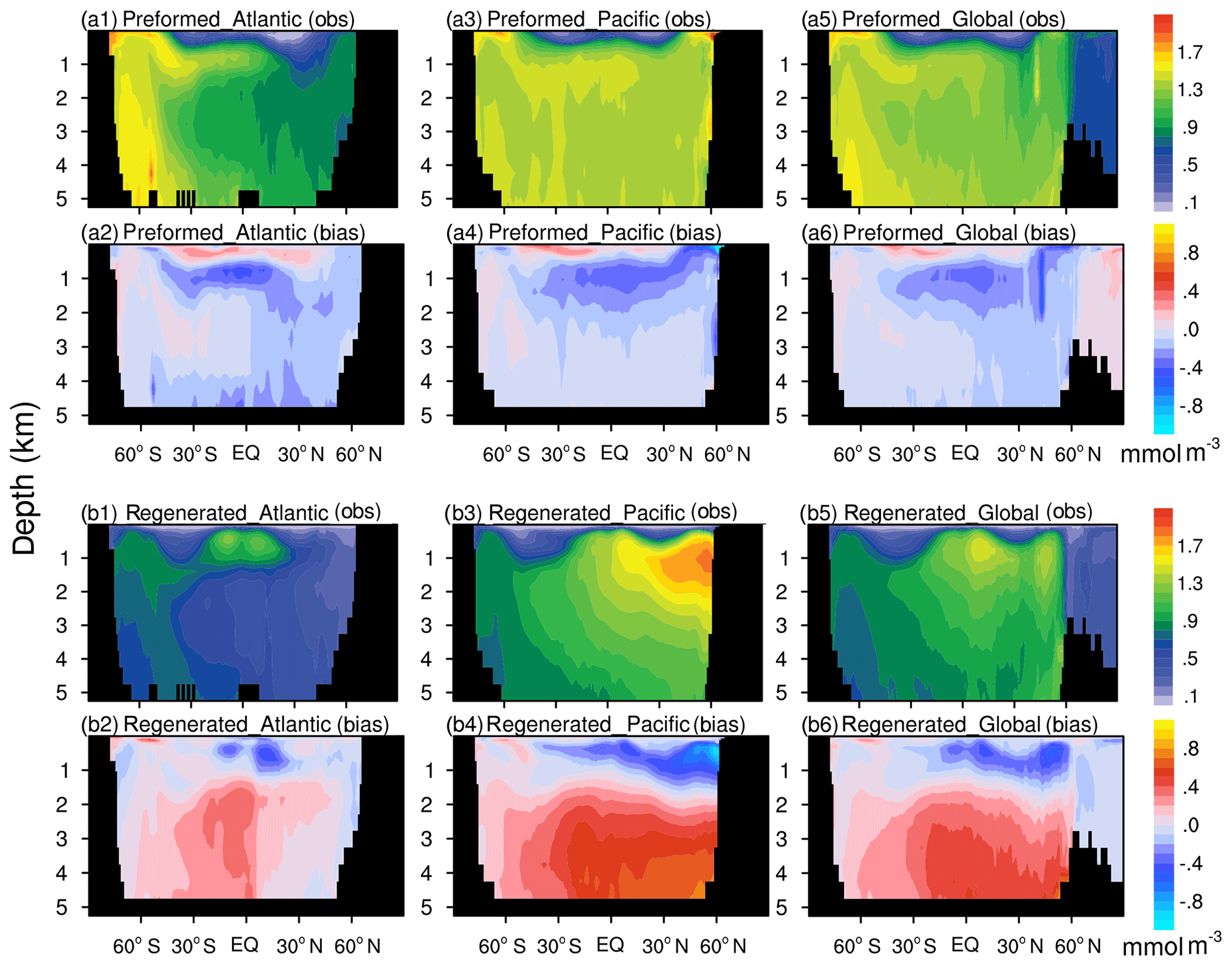
Figure 3 Latitude–depth distributions of the preformed and regenerated phosphate concentration (mmol m⁻³) in the Pacific, Atlantic, and global ocean averaged over 1985 to 2014. The results diagnosed from the WOA18 observation dataset are shown in the first and third rows (a1, a3, a5, b1, b3, b5). The differences (model minus observation) between NESM v3 simulations and observations are shown in the second and the last rows (a2, a4, a6, b2, b4, b6). The panels from (a1) to (a6) show the preformed component, and the panels from (b1) to (b6) show the regenerated component.

The most noticeable biases of regenerated phosphate are found in the deep North Pacific. In the model simulation, the regenerated phosphate in the deep North Pacific is significantly overestimated, and the biases resemble the difference found in latitudinal–depth distributions of nutrients. In the deep ocean, preformed phosphate is only affected by ocean circulation, whereas regenerated phosphate is affected by both circulation and remineralization. In the deep ocean, the NESM v3 simulates the preformed phosphate well but overestimates the regenerated phosphate, indicating that the overestimated nutrients in the North Pacific deep ocean are mainly caused by biological processes.

Next, we present the NESM v3 simulated patterns of nutrient limitation. As shown in Fig. 4, the limiting patterns of nanophytoplankton and diatoms are similar in the tropical- and temperate-latitude oceans. Iron is the most limiting nutrient for both nanophytoplankton and diatoms in the eastern Pacific and the Southern Ocean. Nitrate and phosphate are the most limiting factors in the Indian Ocean, subtropical western Pacific, and the tropical Atlantic. In high-latitude oceans, nanophytoplankton is mostly limited by the available light and temperature, whereas diatoms are mostly limited by silicate. The NESM v3 simulated limiting pattern broadly agrees with the results diagnosed from the IPSL-CM4A-LOOP (Schneider et al., 2008) and the Community Earth System Model-Biogeochemistry (CESM1-BGC; Moore et al., 2013), except that the iron limitation diagnosed from the NESM v3 is stronger in the Pacific and the Southern Ocean.

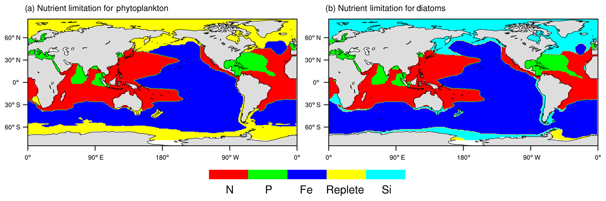
Figure 4 Diagnosed patterns of nutrient limitation from the NESM v3 simulation (FC-HistSSP). The limitation maps are shown over the annual timescale averaged over the years 1985 to 2014 for phytoplankton (a) and diatoms (b). Different colors represent different factors that most limit phytoplankton growth. Replete means nutrient concentrations are sufficient for phytoplankton growth (the growth rate is greater than 90 % of their maximal growth rate).

3.2 Biological production

Figure 5 compares the modeled spatial distributions of the annual mean surface chlorophyll concentration from 1998 to 2014 with that in SeaWiFS observational data, GlobColour merged data, and OCCCI merged data. In the NESM v3, chlorophyll in both nanophytoplankton and diatoms is parameterized based on the photo-adaptive model (Geider et al., 1997) in which chlorophyll is regulated by the chlorophyll-to-carbon ratio, growth of phytoplankton biomass, mortality, aggregation, and zooplankton grazing. The large-scale pattern of the simulated ocean chlorophyll concentration broadly agrees with observations, with high levels of chlorophyll in the subarctic Pacific Ocean and North Atlantic (>1 mg Chl m³) and intermediate levels of chlorophyll in the Southern Ocean (∼0.5 mg Chl m³). Also, the observed relatively high chlorophyll concentration in the equatorial Pacific (∼0.3 mg Chl m³) surrounded by low-chlorophyll-concentration seawater over the subtropical oceans (<0.1 mg Chl m³) is reproduced by the model. The high chlorophyll concentrations along the extratropical coastal regions are broadly captured by the NESM v3. However, the model underestimates the chlorophyll concentration in the tropical coastal regions, especially in the tropical Indian Ocean, Maritime Continent, and the tropical Atlantic. This underestimation is partly associated with the deficiencies in modeled coastal dynamics, which are usually not represented well by coarse global ocean models (Aumont et al., 2015). It is reported that the observed chlorophyll distribution in the coastal region is better reproduced when PISCES is coupled to a higher-resolution ocean circulation model (Lee et al., 2000; Hood et al., 2003; Koné et al., 2009). Also, the model underestimates the chlorophyll concentration in the northern Indian Ocean. This underestimation of chlorophyll is associated with the underestimation of nutrients over the Indian Ocean (Fig. 1) that inhibits phytoplankton growth.

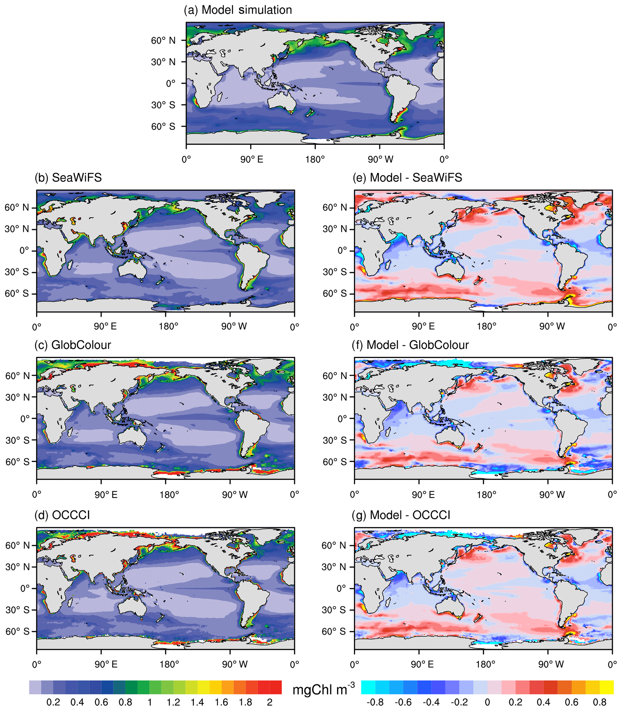
Figure 5 Annual mean surface chlorophyll concentration (mg Chl m⁻³) from the NESM v3 FC-HistSSP simulations (a; averaged over 1998 to 2014), the SeaWiFS dataset (b; averaged over 1998 to 2010), the GlobColour merged dataset (c; averaged over 1998 to 2014), and the OCCCI merged dataset (d; averaged over 1998 to 2014). The biases between the NESM v3 simulation and observations are shown in the (e), (f), and (g).

In the Southern Ocean where the seawater is typically characterized by high nutrient and low chlorophyll levels (Lin et al., 2016), noticeable discrepancies in chlorophyll concentrations are seen among different observationally based datasets, which are associated with different algorithms used for these products. For example, in the Southern Ocean, the chlorophyll concentration derived from reflectance by standard algorithms tends to be underestimated by a factor of about 2 to 2.5 (Kahru and Mitchell, 2010). Compared to the three observational data-based estimates, the NESM v3 overestimates the chlorophyll concentration in the Pacific and Indian parts of the Southern Ocean. In the Atlantic part of the Southern Ocean, the modeled chlorophyll concentration is within the range of observational estimates, higher than the SeaWiFS but lower than the GlobColour and OCCCI.

Figure 6 shows the annual mean spatial distributions of vertically integrated NPP from 2003 to 2014. Three different algorithms, including VGPM, Eppley-VGPM, and CbPM, are used to estimate the NPP based on MODIS observations. Similar to the CbPM, the NESM v3 simulates NPP as the product of phytoplankton biomass and the growth rate, while the VGPM and Eppley-VGPM describe NPP as the product of chlorophyll and photosynthetic efficiencies. However, the formulation of the growth rate in the NESM v3 is more complex than that in CbPM, which involves chlorophyll, nutrient availability, temperature, respiration, and PAR.

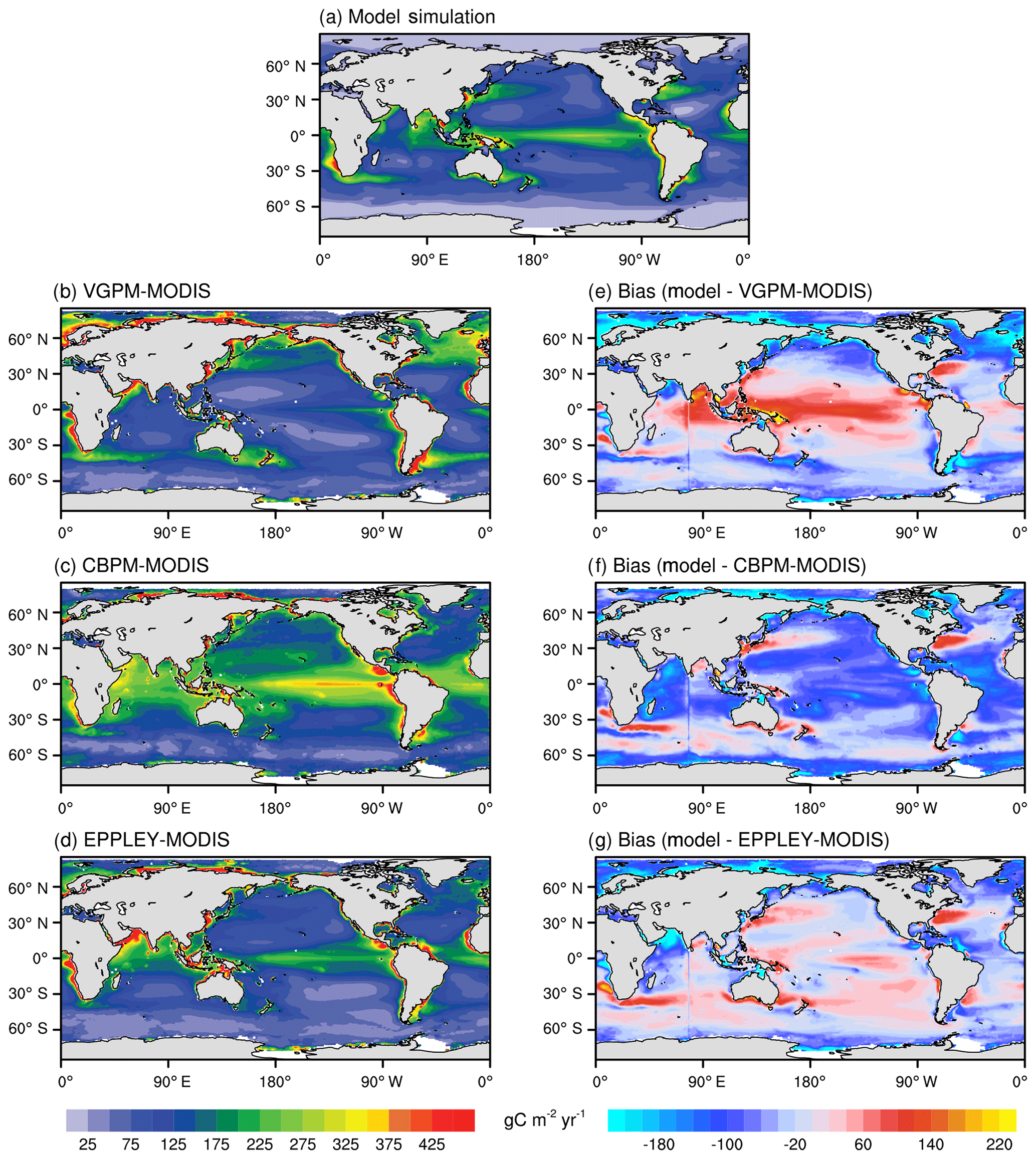
Figure 6 Annual mean distributions of vertically integrated net primary production (g C m⁻² yr⁻¹) averaged from 2003 to 2014 from the NESM v3 FC-HistSSP simulations (a) and MODIS observation-based estimates (b: VGPM-MODIS; c: CBPM-MODIS; d: Eppley-MODIS). The biases of model simulations and observations are shown in panels (e, f, g).

The formulation of the growth rate in the NESM v3 follows Eppley (1972), i.e., the growth rate is higher in high-temperature regions, while there is no temperature dependence in the VGPM. Therefore, compared to VGPM, the NESM v3 estimates more NPP in low-latitude oceans and less NPP in high-latitude oceans (Fig. 6e). The spatial distribution of the NESM v3 simulated vertically integrated NPP resembles Eppley-VGPM and CbPM estimates (Fig. 6a, c, d). The NESM v3 broadly reproduces the observed spatial pattern of NPP distribution, with high NPP in the eastern equatorial Pacific and Maritime Continent and low NPP in the subtropical Pacific and high-latitude oceans. Also, the NESM v3 broadly captures the high concentrations of NPP in low-latitude coastal regions. Although the global pattern of NPP broadly agrees with the observation-based estimates, the PCC between model simulations and Eppley-VGPM is only 0.5, indicating that some local features are not well described in the NESM v3. Compared to CbPM and Eppley-VGPM, the NESM v3 significantly underestimates NPP in the Indian Ocean. The NESM v3 also underestimates NPP in the eastern coastal areas of the United States and the Arctic coastal areas.

Averaged from 2003 to 2014, the globally integrated ocean NPP from the NESM v3 simulation is 45.1 PgC yr⁻¹ compared with data-based estimates of 38 to 65 PgC yr⁻¹ (Buitenhuis et al., 2013). The large range of data-based estimates of global NPP is a result of different satellite observations and different algorithms for the NPP estimation (Longhurst et al., 1995; Antoine et al., 1996; Behrenfeld and Falkowski, 1997b; Behrenfeld et al., 2005). Global NPP simulated by CMIP5 models also shows a wide range of values from 30.9 to 78.7 PgC yr⁻¹ (Bopp et al., 2013). The NESM v3 simulated global NPP is within the range of data-based estimates and current CMIP5 model estimates. Of the NESM v3 simulated global ocean NPP, 20 % is contributed by diatoms, and 80 % is contributed by nanophytoplankton. For comparison, from the data-based estimates, 7 % to 32 % of the total NPP is associated with diatoms (Uitz et al., 2010; Hirata et al., 2011), while ocean biogeochemical models estimate that 15 % to 30 % of global NPP is from diatoms (Aumont et al., 2003; Dutkiewicz et al., 2005; Yool et al., 2011).

3.3 Dissolved inorganic carbon and alkalinity

Figures 7 and 8 display the modeled and observed spatial distributions of alkalinity and DIC averaged over the upper ocean (0–100 m) and the zonally averaged section in the Pacific Ocean, Atlantic Ocean, and the global ocean during the period from 1985 to 2014. The model's skill in simulating upper-ocean alkalinity is moderate (PCC =0.56). The model reproduced the observed high alkalinity in the subtropical surface oceans, and the modeled global upper-ocean mean alkalinity has a minor negative bias of 0.45 %. The major discrepancies are seen in the Southern Ocean and the subarctic Pacific, with a positive bias of more than 80 mmol m⁻³. In high-latitude oceans, convective mixing of alkalinity-rich deep water is an important factor controlling upper-ocean alkalinity, and SST can be used as a proxy for convective mixing (Lee et al., 2006). An underestimation of SST of 1 ^∘C is simulated in high-latitude oceans (figures not shown), indicating a stronger convective mixing, which may explain the overestimated alkalinity in high-latitude oceans. The alkalinity has a negative bias of more than 60 mmol m⁻³ near the Maritime Continent, where the alkalinity concentration is usually related to salinity (Lee et al., 2006). Cao et al. (2018) found that the NESM v3 simulates excessive precipitation over the Maritime Continent, which results in the underestimation of salinity by 2 PSU.

Figure 7 Annual mean distributions of upper-ocean mean (0–100 m) alkalinity (mmol m⁻³) (a, b) and DIC (mmol C m⁻³) (c, d) averaged from 1985 to 2014 from the NESM v3 simulations (a, c) and GLODAP v2 (b, d). The biases of the NESM v3 simulations and observations are shown in panels (e, f).

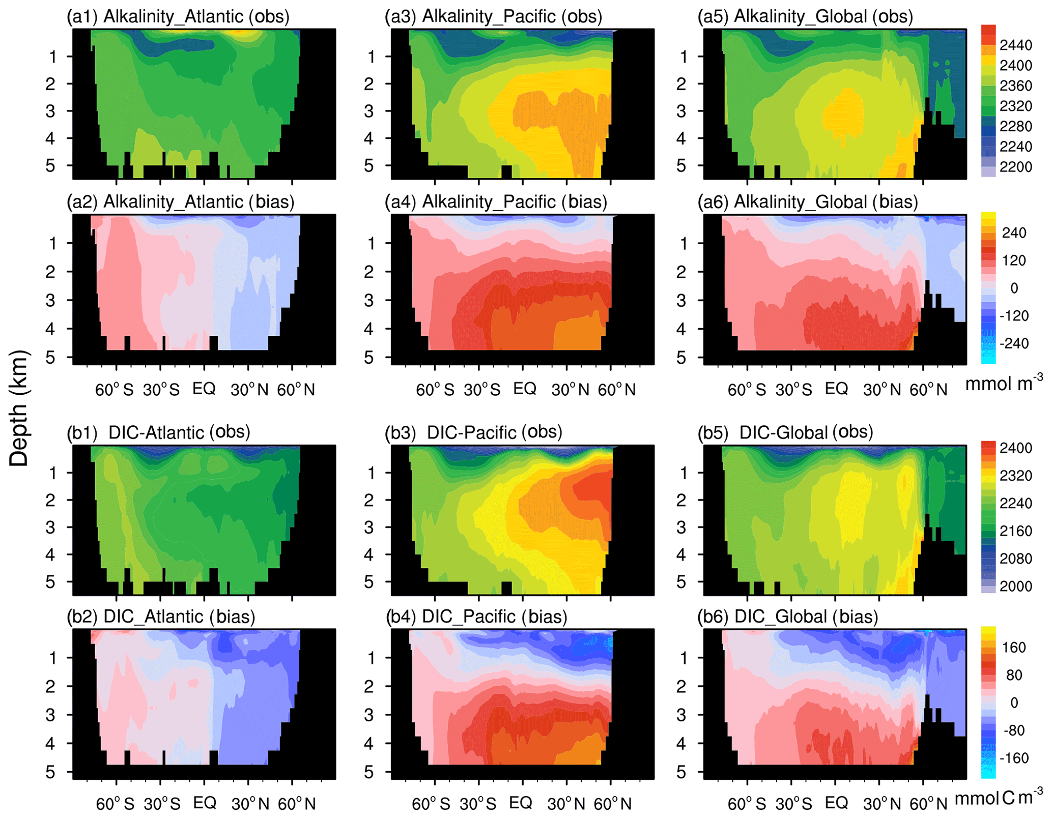
Figure 8 The latitude–depth distributions of alkalinity (a; mmol m⁻³) and DIC (b; mmol C m⁻³) averaged from 1985 to 2014 from the FC-HistSSP simulation are compared with GLODAP v2 observations. The observations are shown in the first and third rows (a1, a3, a5, b1, b3, b5), whereas the biases (model minus observation) are shown in the second and last rows (a2, a4, a6, b2, b4, b6).

NESM v3 simulates the large-scale pattern of the observed DIC well (PCC =0.78), with a high DIC concentration in the middle- to high-latitude Atlantic and a low DIC concentration in the middle- to low-latitude Pacific and the Indian Ocean. The model-simulated global mean upper-ocean DIC has a minor positive bias of 0.27 %. Although the global pattern of DIC is different from alkalinity, their model–observation bias patterns are similar (Fig. 7e, f). The largest positive DIC bias of more than 80 mmol C m⁻³ is simulated in the Southern Ocean and subarctic Pacific, while a negative bias of more than 80 mmol C m⁻³ is simulated in the Maritime Continent.

In the Atlantic, the large-scale patterns of the latitudinal–depth distributions of DIC and alkalinity simulated by the model broadly agree with observations. Both alkalinity and DIC are slightly overestimated in the South Atlantic and underestimated in the North Atlantic. Apparent biases of DIC and alkalinity are seen in the deep North Pacific. One noticeable pattern of the observed DIC and alkalinity is that their maximum concentrations are around 2000–3000 m in the North Pacific Ocean, which the model fails to reproduce. The model also overestimates DIC storage in the deep Pacific Ocean. The mismatches between the model simulation and observations, i.e., an underestimation of DIC and alkalinity concentrations in the upper 1000 m of depth and an overestimation of their concentrations in the deep ocean, resemble those of nutrients. It indicates that modeled discrepancies of alkalinity and DIC may also be attributed to excessive deep and active remineralization processes, which release a large amount of dissolved carbon in the deep ocean.

3.4 Assessment of biogeochemical fields by Taylor diagram

Figure 9 compares the spatial patterns of the NESM v3 and IPSL simulated biogeochemistry-related fields with corresponding observations using a Taylor diagram (Taylor, 2001). In summary, model-simulated statistical patterns of the nutrients in the upper ocean compare well with observations, whereas the simulated spatial patterns of chlorophyll, primary production, and alkalinity show larger discrepancies from observations. It is noted that chlorophyll and NPP are not directly observed but diagnosed from the observation-based data, and thus their estimations are subject to considerable uncertainties. Compared with biogeochemical fields in IPSL, which shares the same marine biogeochemical cycle component with NESM v3, the NESM v3 has comparable skill in reproducing the spatial distributions of nutrients and chlorophyll but less skill in reproducing DIC and alkalinity, with relatively larger NSDs.

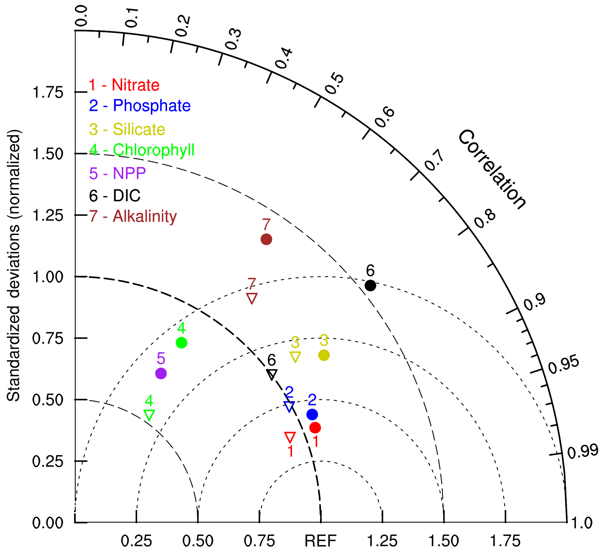
Figure 9 The Taylor diagram compares the statistical patterns of annual mean biogeochemical fields averaged over the upper 100 m ocean between the NESM v3 simulation (FC-HistSSP) and corresponding observations, including nitrate, phosphate, silicate, alkalinity, chlorophyll concentration, and vertically integrated net primary production. Nutrient concentrations are compared with WOA 18; the DIC and alkalinity concentrations are compared with GLODAP v2; NPP is compared with the CbPM; chlorophyll is compared with SeaWiFS. All fields are normalized by the standard deviation of corresponding observations. Thus, observation fields have a standard deviation of 1, which is represented by REF. The distance between the model points and the reference point indicates the root mean square (RMS) difference between the model simulation and observations. The solid cycle represents the results diagnosed from the NESM v3, and the triangle represents the results from the IPSL, which shares the same marine biogeochemical model as the NESM v3. The NPP of IPSL is not shown here.

We also examine other CMIP5 model results documented in previous studies (Moore et al., 2013; Anav et al., 2013; Tjiputra et al., 2013; Séférian et al., 2013). For different biogeochemical fields, different models show different skills. For example, PCCs between nutrients and observations in CESM1-BGC are about 0.8, which is lower than in the NESM v3, but CESM has a better representation of chlorophyll (Moore et al., 2013). Nevertheless, the NESM v3 shows comparable skill in simulating upper-ocean biogeochemical fields with other CMIP5 models.

3.5 Oceanic anthropogenic CO₂ uptake during the historical period

In this section, we compare the NESM v3 simulated anthropogenic carbon uptake (FC-HistSSP simulation) during the historical period against available observation-based estimates.

First, we compared the NESM v3 simulated sea–air CO₂ flux against available observations for the reference year of 2000 (Takahashi et al., 2009). As shown in Fig. 10, the NESM v3 realistically reproduces the large-scale pattern of the observed sea–air CO₂ flux with CO₂ outgassing in the equatorial oceans and uptake in the middle- to high-latitude oceans (PCC =0.71 and NSDs =1.04). For both observations and model results, strong CO₂ uptake is found in the northern Atlantic where sea surface temperature is low and the formation of deep water is active. Compared to the data-based estimates, the modeled sea–air CO₂ flux is overestimated in the tropical Pacific, the Southern Ocean, and the North Pacific (near 30^∘ N). Also, the model underestimates the sea–air CO₂ flux in the high-latitude oceans (Fig. 9c and d). The globally integrated ocean uptake flux from observations is 1.6±0.9 PgC yr⁻¹ for the reference year of 2000 (Takahashi et al., 2009), whereas the value is 2.8 PgC yr⁻¹ from the model simulation. The difference between the model and observations mainly originates from the model-simulated positive bias in the preindustrial steady-state oceanic CO₂. In the NESM v3, the preindustrial steady state of total oceanic CO₂ uptake is 1.0 PgC yr⁻¹ compared with the data-based value of 0.4±0.2 PgC yr⁻¹ (Takahashi et al., 2009). Taking the preindustrial steady state into consideration, the total oceanic anthropogenic CO₂ uptake flux in the year 2000 is 1.8 PgC from the model simulation compared to the value of 2.0±1.0 PgC from the observation (Takahashi et al., 2009).

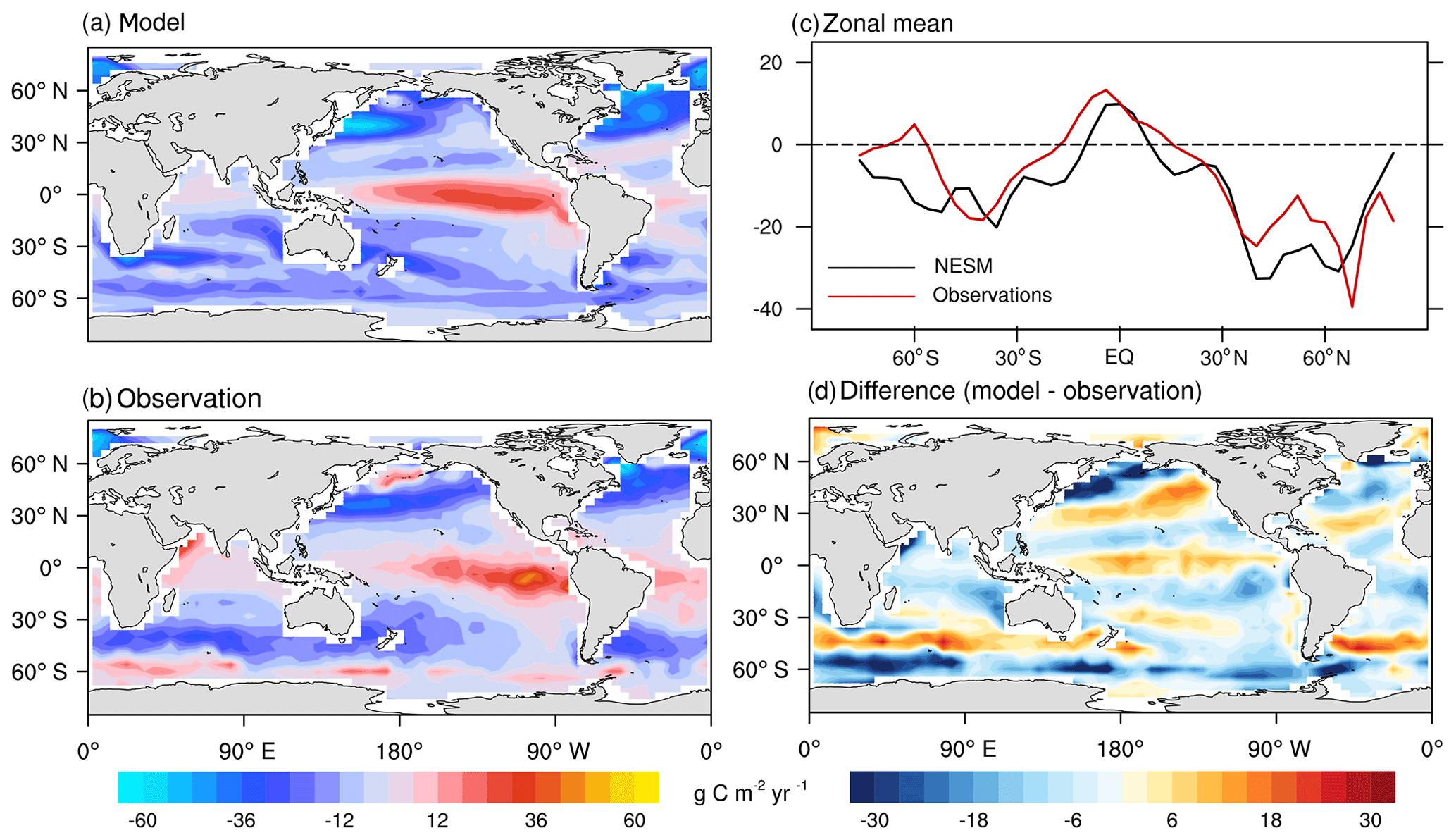
Figure 10 Model-simulated sea–air CO₂ flux (g C m⁻² yr⁻¹) in the year 2000 compared with data-based observational estimates (Takahashi et al., 2009). Spatial distributions of the model simulation (a), observation (b), zonal mean pattern of model simulation and observation (c), and the difference between the model and observation (d). Positive values represent CO₂ flux out of the ocean, and negative values represent CO₂ flux into the ocean.

Then, we compared the NESM v3 simulated anthropogenic CO₂ budget with the data-based estimates provided by the Fifth Assessment Report of the Intergovernmental Panel on Climate Change (IPCC AR5) (Table 1). The model-simulated ocean uptake of anthropogenic CO₂ is slightly lower than that from the IPCC AR5 but within the estimated uncertainty range. From the preindustrial era to the year 2011, the NESM v3 simulated cumulative oceanic CO₂ uptake is 137.2 PgC compared with IPCC data-based estimates of 155±30 PgC (Ciais et al., 2013). The decadal mean oceanic anthropogenic CO₂ uptake diagnosed from the FC-HistSSP run increased from 1.7 to 2.3 PgC yr⁻¹ from the 1980s to the 2000s, whereas the observation ranges from 2.0±0.7 to 2.4±0.7 PgC yr⁻¹. From the year 1870 to 2016, the modeled cumulative CO₂ uptake is 149 PgC compared to the recent estimate of 150±20 PgC (Le Quéré et al., 2018).

Model-simulated vertically integrated column inventories of anthropogenic DIC (FC-HistSSP relative to the CTRL simulation) from 2000 to 2004 and from 1992 to 1996 are compared with GLODAP v2 and GLODAP v1 (Fig. 11), respectively. Compared with GLODAP v2, the NESM v3 reasonably captures the large-scale distribution of observed anthropogenic DIC. The largest inventory in the 2000s of more than 100 mol C m⁻² is simulated in the northern Atlantic where SST is low and deepwater formation is active. In the model simulation from 2000 to 2004, the North Atlantic stores 20.8 % of the global oceanic anthropogenic carbon, whereas it is 17.6 % in the GLODAP v2. In other ocean basins, the large inventory is mainly found in the middle-latitude areas near 30^∘ N and 30^∘ S for both model simulations and observations. In the NESM v3 simulations, from 2000 to 2004, 58.9 % of the global oceanic anthropogenic carbon is stored in the Southern Ocean compared to the value of 62.6 % in the GLODAP v2.

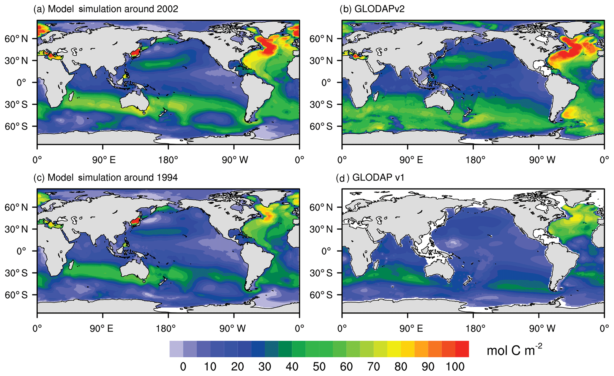
Figure 11 Vertically integrated column inventory of anthropogenic DIC (mol C m⁻²) from the simulation (a, c), GLODAP v2 (b), and GLODAP v1 (d). Model simulation results are averaged from 2000 to 2004 (a, represent the period around 2002) and from 1992 to 1996 (c, represent the period around 1994). The anthropogenic DIC from GLODAP v2 is normalized to the year 2002 (b), while that from GLODAP v1 is normalized to the year 1994 (d).

One noticeable discrepancy between the GLODAP v2 and model simulation is found south of 50^∘ S. Only 8.3 % of the global oceanic anthropogenic DIC inventory is simulated by the model in this region, whereas the value is 15.5 % in the GLODAP v2. However, the vertically integrated anthropogenic DIC concentration is also low in the Southern Ocean (south of 50^∘ S) in the GLODAP v1, accounting for only 9.9 % of the global inventory. Anthropogenic DIC in the GLODAP is diagnosed by a crude application of the transit time distribution method, and thus the results are subject to considerable uncertainties (Lauvset et al., 2016).

Figure 12 shows the latitudinal–depth distributions of the anthropogenic DIC concentration (FC-HistSSP relative to the CTRL simulation) in the Atlantic, Pacific, and the global ocean from the model simulation and GLODAP v2. The observed high concentrations (more than 51 mmol C m⁻³) in near-surface waters and low concentrations (less than 3 mmol C m⁻³) in most of the deep ocean (the Pacific and the middle- to low-latitude Atlantic) are simulated by the NESM v3. For both data-based estimates and model simulations, a substantial amount of anthropogenic CO₂ has penetrated down to the ocean interior as deep as 1000 m of depth, with two penetration tongues near 30^∘ N and 40^∘ S, and the deepest penetration of anthropogenic DIC is found in the northern Atlantic. Deep penetration of anthropogenic DIC is typically associated with convergence zones in temperate and high-latitude oceans where vertical mixing is strong (Sabine et al., 2004). Similar to the vertically integrated inventory of anthropogenic DIC (Fig. 11), the major discrepancy of anthropogenic DIC in the latitudinal–depth distribution is also found in the southern Atlantic south of 50^∘ S where the model greatly underestimates the anthropogenic DIC in the entire ocean column.

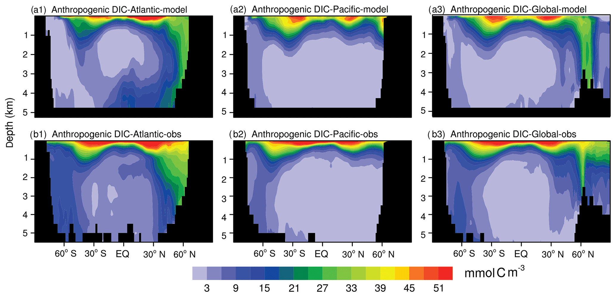
Figure 12 Zonal mean latitude–depth distributions of anthropogenic DIC (mmol C m⁻³) from the model simulation (a1: Atlantic, a2: Pacific, and a3: Global) and data-based estimates (GLODAP v2) (b1: Atlantic, b2: Pacific, and b3: Global). Model simulation results are averaged from the year 2000 to 2004 (a), while the observation is normalized to the year 2002 (b).

3.6 Sensitivity of the oceanic CO₂ uptake to increasing atmospheric CO₂ and global warming

The ocean carbon cycle is regulated by changes in atmospheric CO₂ and the physical climate (Doney et al., 2004). Increasing atmospheric CO₂ affects oceanic CO₂ uptake directly. Meanwhile, global warming also affects the ocean carbon cycle via changes in climate and biological rates (Gregory et al., 2005; Steinacher et al., 2010; Pierce et al., 2012; Olonscheck et al., 2013; Lewandowska et al., 2014). In this section, we first present the NESM v3 simulated physical climate change and oceanic CO₂ uptake under the historical and SSP5–8.5 scenarios. Then, we present the NESM v3 simulated response of the ocean carbon uptake to increasing atmospheric CO₂ and global warming in the SSP5–8.5 and 1ptCO₂ runs.

3.6.1 NESM v3 simulated physical climate change under historical and SSP5–8.5 scenarios

Figure 13 shows the NESM v3 simulated changes (relative to the control simulation) in the global annual mean surface air temperature (SAT), mixed layer depth (MLD), and intensity of the Atlantic meridional overturning circulation (AMOC) from 1850 to 2100 under the historical and SSP5–8.5 scenarios. Changes in SAT, MLD, and AMOC in the RC-HistSSP and FC-HistSSP simulations are almost the same, while those changes in the BC-HistSSP simulation are rather small. In the FC-HistSSP simulation, the annual mean SAT anomaly averaged over the years from 2080 to 2100 (relative to the period of 1986–2005) is 4.6 K, which is at the higher end of the CMIP5 model results (2.6–4.7 K) under the RCP8.5 scenario (Collins et al., 2013; Knutti and Sedláček, 2013). It is noted that the CMIP6 input forcing is used in this study, and the atmospheric CO₂ concentration at the end of the 21st century in the SSP5–8.5 is about 10 % higher than that in the RCP8.5 scenario. Also, we can see a slight increase in SAT in BC-HistSSP (Fig. 13a), which is caused by the non-CO₂ GHG change. Compared with the preindustrial era, by the end of the 21st century (averaged over the years 2091 to 2100), the SAT in the FC-HistSSP, RC-HistSSP, and BC-HistSSP simulations increased by 6.0, 6.0, and 0.8 K, respectively.

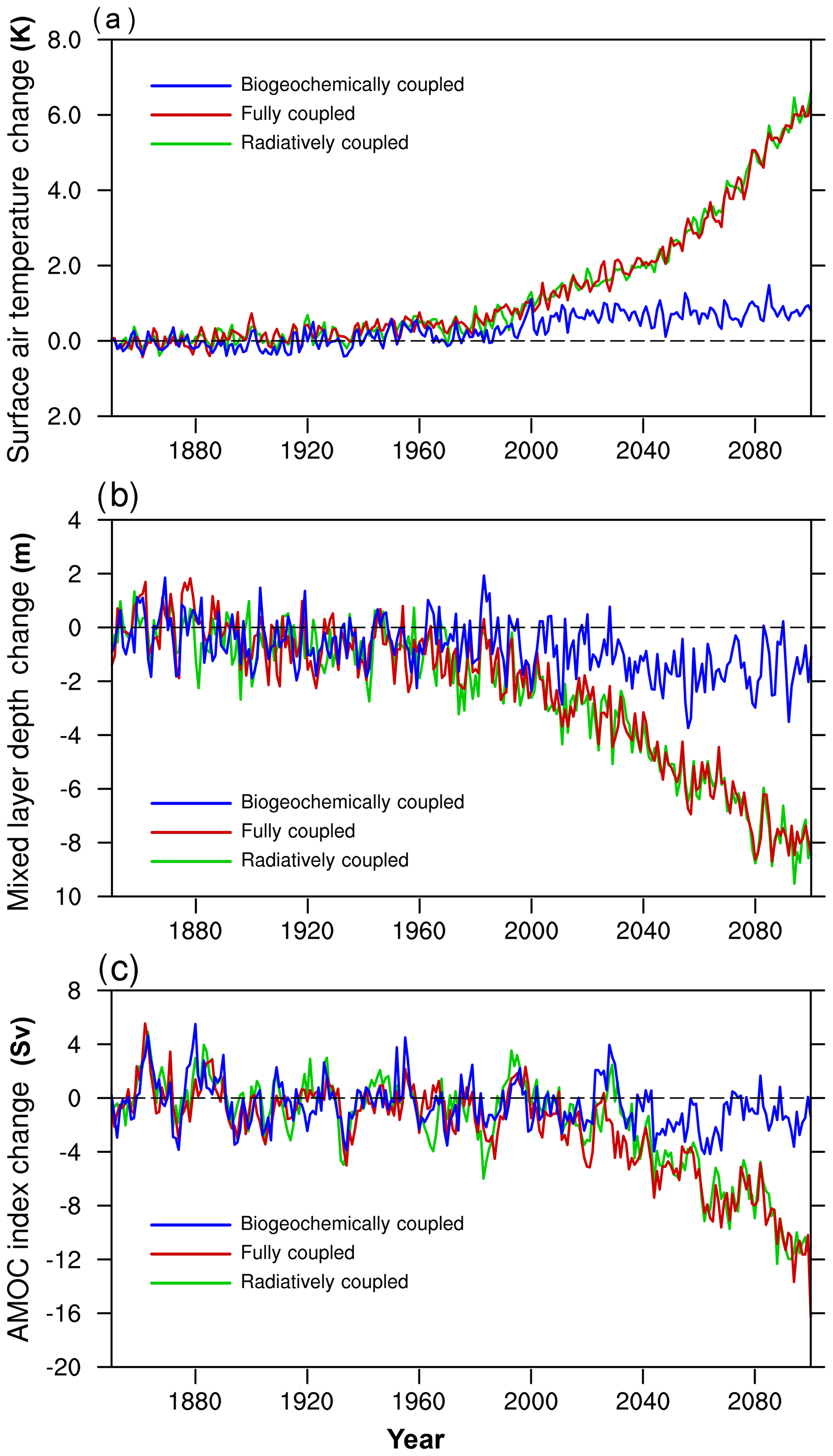
Figure 13 Time series of changes in climate fields (relative to the control simulation) from 1850 to 2100 for BC-HistSSP, FC-HistSSP, and RC-HistSSP. (a) Global and annual mean surface air temperature (K), (b) global and annual mean mixed layer depth (in meters; the mixed layer depth is defined to be the depth at which the difference in potential density is 0.01 kg m⁻³ relative to the sea surface), and (c) Atlantic meridional overturning circulation index (Sv; maximum zonal mean stream function in the Atlantic Ocean at 30^∘ N).

Modeled MLD decreases from the 1980s. Compared with the preindustrial era, by the end of the 21st century, MLD in the FC-HistSSP, RC-HistSSP, and BC-HistSSP simulation decreased by 7.9, 8.0, and 1.4 m, respectively. The reduction of the mixed layer depth indicates a more stratified upper ocean. A substantial weakening of AMOC intensity in the FC-HistSSP simulation is projected for the 21st century, which is associated with ocean surface warming and increased freshwater input into the North Atlantic (Gregory et al., 2005). In the preindustrial period, the model-simulated AMOC index at 30^∘ N is 17.5 Sv (1 Sv =10⁶ m³ s⁻¹), which is within the range of 14 to 31 Sv from CMIP5 models (Weaver et al., 2012). In the FC-HistSSP simulation, the modeled annual mean AMOC transport at 30^∘ N averaged over the years 2004 to 2011 is 17.1 Sv, whereas the observation record during the same period from RAPID/MOCHA (Rapid Climate Change–Meridional Overturning Circulation and Heatflux Array) is 17.5±3.8 Sv (Rhein et al., 2013). By the end of the 21st century, the NESM v3 simulates a 54 % reduction of the AMOC (from 17.5 Sv to 8.0 Sv) from the FC-HistSSP simulation, whereas the AMOC reduction under the RCP8.5 scenario from CMIP5 models ranges from 15 % to 60 % (Cheng et al., 2013). The higher atmospheric CO₂ concentration at the end of 2100 in SSP5–8.5 may partly explain the larger AMOC change in this study. Also, Cao et al. (2018) pointed out that the equilibrium climate sensitivity to CO₂ forcing in the NESM v3 is about 10 % higher than that of the CMIP5 ensemble.

3.6.2 NESM v3 simulated oceanic CO₂ uptakes under historical and SSP5–8.5 scenarios

Figure 14 shows the time evolution of the oceanic CO₂ uptake from BC-HistSSP, RC-HistSSP, FC-HistSSP, and the linear sum of BC-HistSSP and RC-HistSSP. In the BC-HistSSP simulation, the global ocean absorbed a total of 662 PgC of anthropogenic CO₂ from the atmosphere by the year 2100. In the RC-HistSSP simulation, the increased sea surface temperature, enhanced ocean stratification, and weakened AMOC all act to decrease CO₂ uptake (Cox et al., 2000; Zickfeld et al., 2008; Roy et al., 2011; Goris et al., 2015; Cao and Zhang, 2017). By the year 2100, the modeled cumulative CO₂ uptake is −35.9 PgC in the RC-HistSSP simulation. In the FC-HistSSP simulation, oceanic CO₂ uptake is affected by both the increase in atmospheric CO₂ and global warming. By the end of the 21st century in FC-HistSSP, simulated cumulative oceanic CO₂ uptake since the preindustrial era is 567 PgC, which is within the ranges of 420 to 600 PgC from CMIP5 model results under the RCP8.5 scenario (Jones et al., 2013). The sum of the simulated oceanic CO₂ uptake from the BC-HistSSP and RC-HistSSP simulations (626 PgC) is larger than that from the FC-HistSSP run (567 PgC), indicating that the effect of increasing atmospheric CO₂ (carbon-concentration sensitivity) and the effect of global warming (carbon-climate sensitivity) on the oceanic CO₂ uptake are not perfectly additive. This nonlinearity was also found in previous studies (Boer and Arora, 2009; Gregory et al., 2009; Schwinger et al., 2014). The NESM v3 simulated nonlinearity (i.e., BC+RC−FC) is 59 PgC by the end of the 21st century, which is larger than the absolute value of the radiative effect on oceanic carbon uptake (−35.9 PgC).

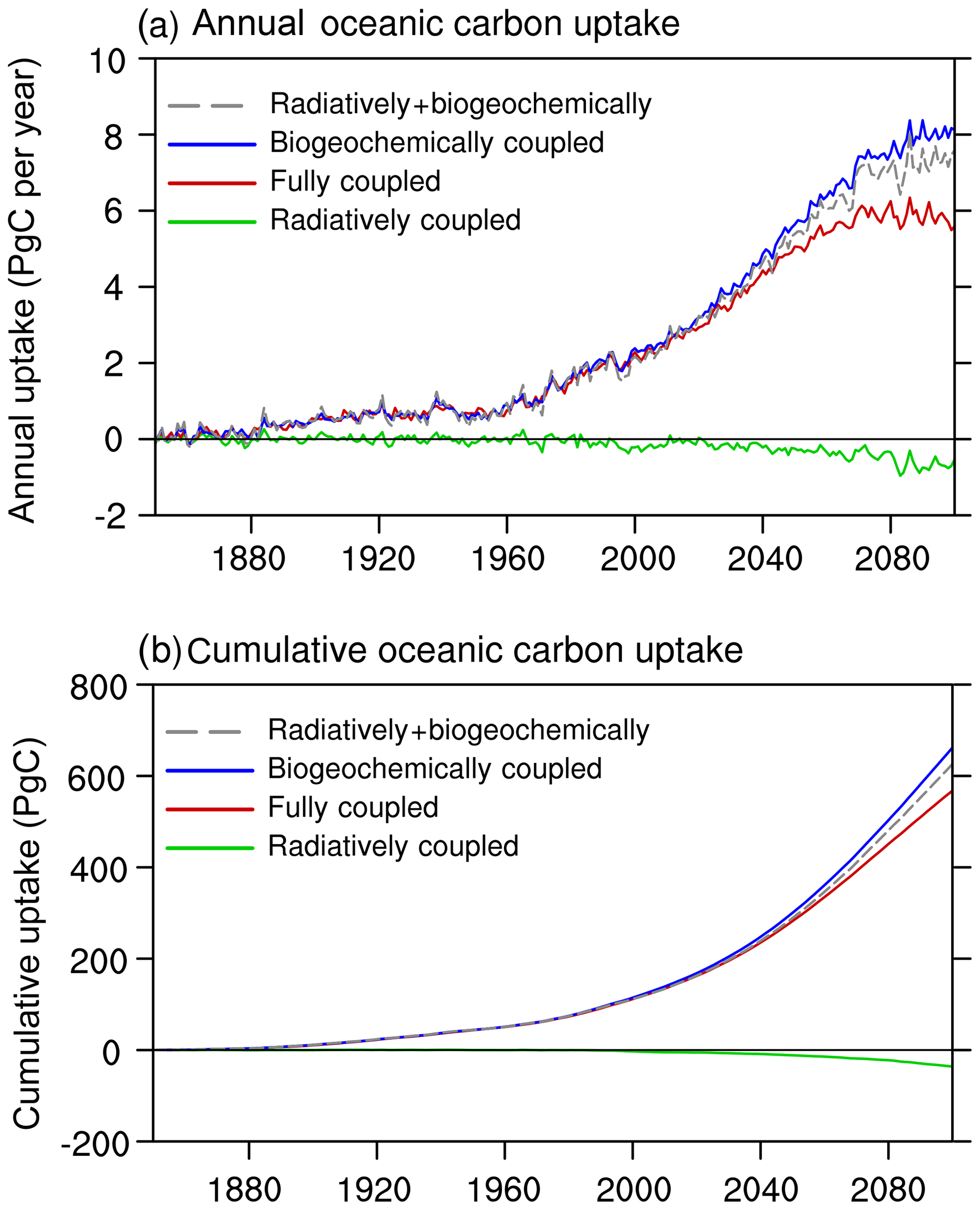
Figure 14 The NESM v3 simulated annual anthropogenic oceanic CO₂ uptake (a; PgC yr⁻¹) and cumulative oceanic CO₂ uptake (b; PgC) for the simulations RC-HistSSP, BC-HistSSP, FC-HistSSP, as well as the linear sum of BC-HistSSP and RC-HistSSP from 1850 to 2100.

To better understand oceanic CO₂ uptake in response to changing atmospheric CO₂ and global warming, Fig. 15 shows the spatial distribution of anthropogenic sea–air CO₂ flux at the end of the 21st century (averaged over the years 2091 to 2100) from the FC-HistSSP, RC-HistSSP, and BC-HistSSP simulations, as well as the difference between the FC-HistSSP simulation and the sum of the RC-HistSSP and BC-HistSSP simulations.

Figure 15 Spatial distributions of anthropogenic sea–air CO₂ flux (g C m⁻² yr⁻¹) at the end of the 21st century (mean of 2091–2100) from the BC-HistSSP (a), RC-HistSSP (b), and FC-HistSSP (c) simulations. Also shown is the difference between the FC-HistSSP simulation and the sum of the RC-HistSSP and BC-HistSSP simulations (FC-RC-BC). Positive values represent CO₂ flux out of the ocean, and negative values represent CO₂ flux into the ocean.

In the BC-HistSSP simulation, the oceanic anthropogenic CO₂ uptake is 8.0 PgC yr⁻¹ at the end of the 21st century. The ocean absorbs atmospheric CO₂ in most regions except for a few scattered grid points at the midlatitudes with slight CO₂ outgassing. The strongest CO₂ uptake of about 150 g C m⁻² yr⁻¹ is found in the North Atlantic, subarctic Pacific, and the Southern Ocean. Results from the RC-HistSSP simulation show CO₂ outgassing in large parts of the global ocean as a result of global warming. In the Arctic Ocean, warming induces a net uptake of CO₂ of 0.07 PgC yr⁻¹ because of the reduced sea ice extent under global warming that allows more open seawater to absorb atmospheric CO₂. In the North Atlantic, the capacity of the ocean to uptake CO₂ is significantly suppressed due to the reduced AMOC. The FC-HistSSP simulation shows the joint effects of increasing atmospheric CO₂ and global warming (Fig. 15c). Net oceanic CO₂ uptake is simulated in most regions, with the strongest uptake in the Southern Ocean, indicating the dominant role of the increasing atmospheric CO₂. CO₂ outgassing is seen in the subtropical Pacific, indicating that the radiative effect dominates the response of oceanic CO₂ uptake in this region.

The nonlinearity of oceanic carbon uptake sensitivity during the 2090s is shown in Fig. 15d. In the NESM v3, the oceanic carbon uptake in the FC-HistSSP simulation is lower than the sum of that in the BC-HistSSP and RC-HistSSP simulations. A relatively large nonlinearity is simulated in the Atlantic north of 45^∘ N (19.8 % of the total nonlinearity) and the Southern Ocean south of 40^∘ S (35.3 % of the total nonlinearity), which is consistent with the findings of previous studies (Zickfeld et al., 2011; Schwinger et al., 2014). The interactions between different background oceanic CO₂ content and global warming can partly explain the nonlinearity. Compared with the RC-HistSSP simulation, in the FC-HistSSP simulation, there is much more carbon in the ocean that is subject to the impact of climate change. As a consequence, in the FC-HistSSP simulation, the increased temperature would have a larger effect on CO₂ solubility and a buffer factor that reduces the ocean's capacity to absorb CO₂ (Yi et al., 2001). Also, reduced ocean circulation and increased ocean stratification would slow down the transport of anthropogenic CO₂ from the surface to the deep ocean. Thus, compared to the BC-HistSSP simulation, slowing ocean ventilation in the FC-HistSSP simulation would cause a larger reduction in oceanic CO₂ uptake.

The above results also indicate that oceanic CO₂ uptake in high-latitude oceans is more sensitive to both the increasing atmospheric CO₂ concentration and global warming than low-latitude oceans, as well as their nonlinear interactions.

3.6.3 Carbon-concentration and carbon-climate sensitivity parameters diagnosed under SSP5–8.5

In this section, we investigate oceanic CO₂ uptake under the framework of the carbon-concentration and carbon-climate sensitivity parameters. Figure 16 shows the change in ocean carbon storage against the change in the atmospheric CO₂ concentration (Fig. 16a) and the global annual mean surface temperature (Fig. 16b). The derived evolution of the carbon-concentration sensitivity parameter β as a function of atmospheric CO₂ concentration and carbon-climate sensitivity parameter γ as a function of the change in temperature is shown in Fig. 16c and d, respectively.

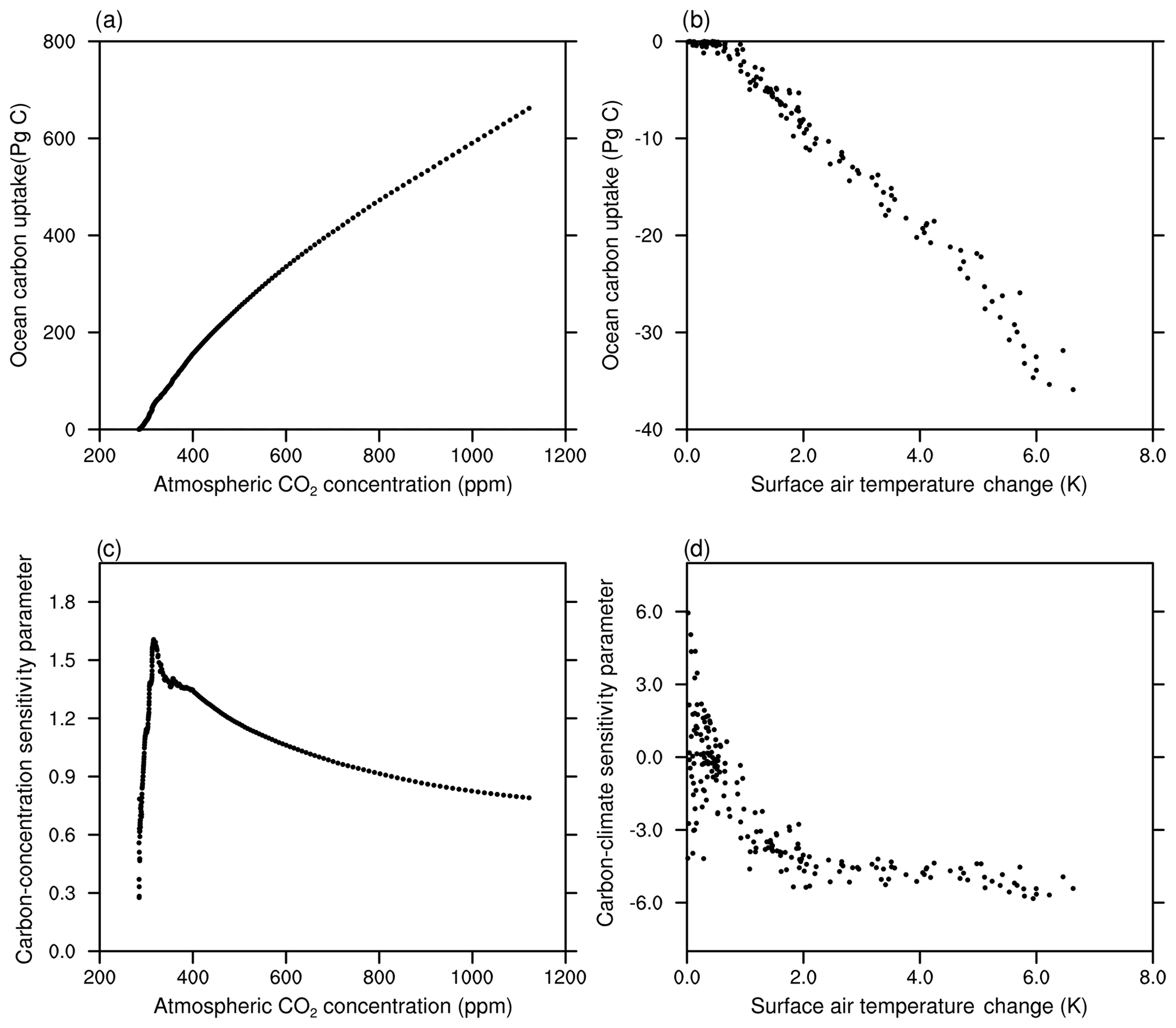
Figure 16 The cumulative oceanic CO₂ uptake against the atmospheric CO₂ in the BC-HistSSP simulation (a) and the global mean surface air temperature change in the RC-HistSSP simulation (b). Also shown is the time evolution of the diagnosed carbon-concentration sensitivity parameter as a function of atmospheric CO₂ (c) and the carbon-climate sensitivity parameter as a function of global mean surface air temperature change (d). All the parameters in this figure are diagnosed from HistSSP scenarios

As shown in Fig. 16, in the BC-HistSSP and RC-HistSSP simulations, the modeled ocean storage of anthropogenic CO₂ scales roughly linearly with atmospheric CO₂ and changes in global mean surface temperature. Increasing atmospheric CO₂ alone increases oceanic CO₂ uptake, whereas increasing temperature alone decreases CO₂ uptake. In the year 2100, the carbon-climate sensitivity parameter γ is −5.4 PgC K⁻¹, while the carbon-concentration sensitivity parameter β is 0.79 PgC ppm⁻¹. The carbon-concentration parameter initially increases with atmospheric CO₂ and then decreases (Fig. 16c). The decreasing trend of β is consistent with the slowdown of the increasing trend of the oceanic CO₂ uptake at the end of the 21st century as a result of decreased oceanic buffer ability (Fig. 16a and c). From 1850 to 2100, the carbon-climate parameter becomes more negative with increasing temperature, indicating that the increase in surface temperature would induce more CO₂ outgassing from the ocean in a warmer world (Fig. 16d). Similar changes in the carbon-climate and carbon-concentration sensitivity parameters are also found in CMIP5 model simulations (Arora et al., 2013). The increased sensitivity of CO₂ outgassing to temperature and the decreased sensitivity of CO₂ uptake to the atmospheric CO₂ concentration indicate that the ocean's ability to absorb atmospheric CO₂ would be weakened with increasing atmospheric CO₂ and global warming.

3.6.4 Carbon-concentration and carbon-climate sensitivity parameters from 1ptCO₂ runs

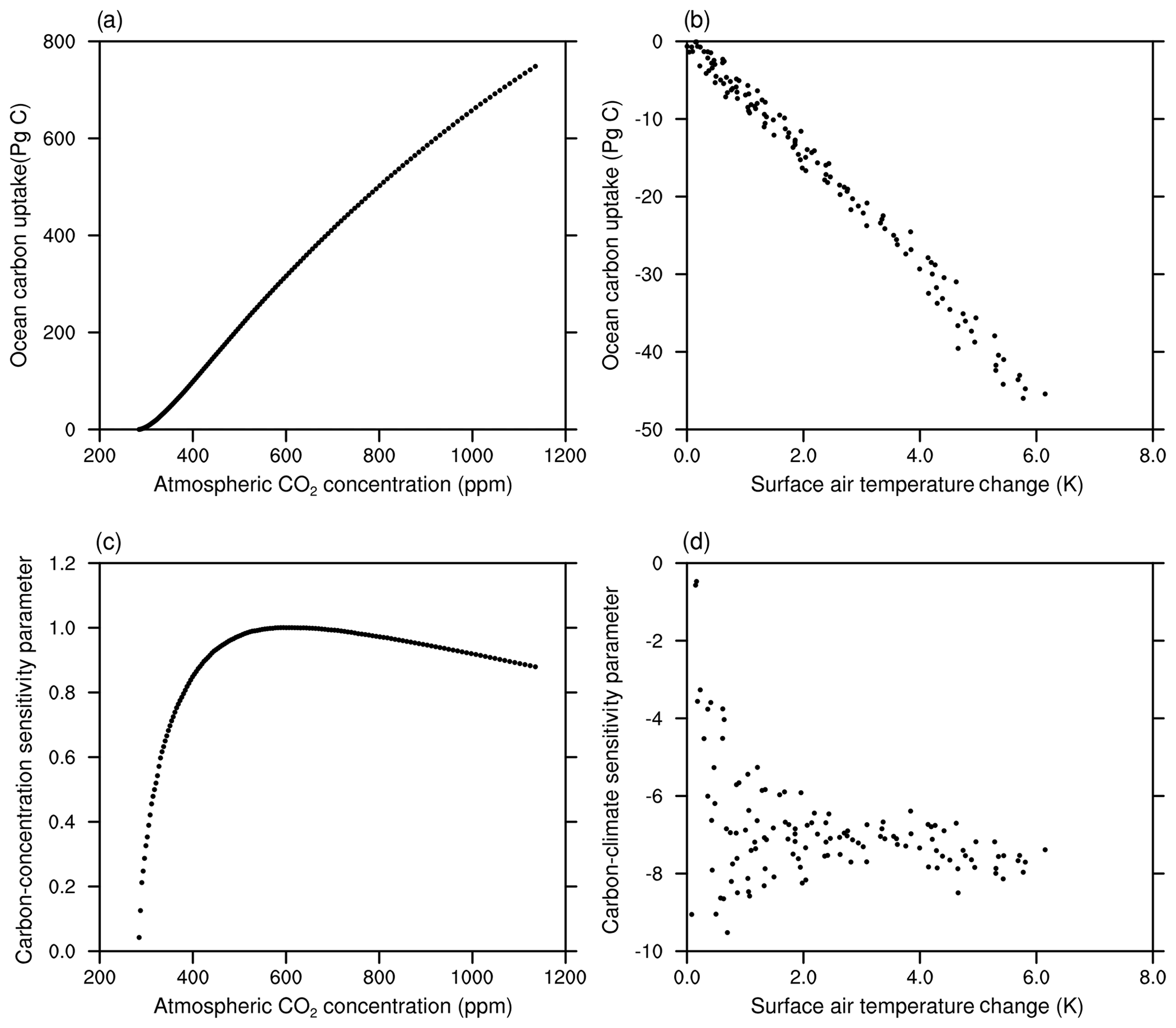
In this section, we compare the carbon sensitivity parameters diagnosed from the 1ptCO₂ experiments between the NESM v3 and CMIP5 models. The total CO₂ uptake during the 140 years in FC-1ptCO₂ is 636 PgC, while the results from CMIP5 models range from 533 to 676 PgC. The sum of the total CO₂ uptake in RC-1ptCO₂ and BC-1ptCO₂ is 702 PgC, which is larger than that in FC-1ptCO₂. The simulated nonlinearity (i.e., BC-1ptCO₂ + RC-1ptCO₂ − FC-1ptCO₂) is about 10.3 % of the total CO₂ uptake in FC-1ptCO₂, which is at the higher end of the nonlinearity estimated for CMIP5 models (3.6 %–10.6 %; Schwinger et al., 2014). Figure 17 shows the simulated β and γ in the 1ptCO₂ experiments. At the end of the 1ptCO₂ experiments, the diagnosed value of β from CMIP5 models ranges from 0.69 to 0.91 PgC ppm⁻¹, with a multi-model mean value of 0.80 PgC ppm⁻¹. For comparison, the β diagnosed from the NESM v3 simulations is 0.88 PgC ppm⁻¹. In the 1ptCO₂ experiment, the β simulated by the NESM v3 tends to decrease when the atmospheric CO₂ concentration increases to ∼550 ppm, which is consistent with that in CMIP5 models. At the end of the 1ptCO₂ experiments, the diagnosed value of γ from CMIP5 models ranges from −2.4 to −12.1 PgC K⁻¹. The larger spread of γ is associated with the spread of the model-simulated climate change and the dependency of carbon cycle processes on climate change. For comparison, the diagnosed γ parameter from the NESM v3 simulation is −7.9 PgC K⁻¹.

Figure 17 Same as Fig. 16, but for the 1ptCO₂ runs.

4 Discussion and conclusion

In this study, we evaluated the performance of NESM v3 in simulating the present-day ocean biogeochemical cycle and historical and future oceanic carbon uptake. We also investigated the response of oceanic CO₂ uptake to the individual and combined effect of increasing atmospheric CO₂ and CO₂-induced warming under the SSP5–8.5 and 1ptCO₂ scenarios. The strengths and limitations of the NESM v3 are analyzed and documented.

The NESM v3 simulates the large-scale patterns of observed upper-ocean nutrients reasonably well, with PCCs larger than 0.8 and NSDs close to 1.0 (Figs. 1 and 9). The high nutrient concentrations in the eastern Pacific, subarctic Pacific, and the Southern Ocean are reproduced in the model (Fig. 1). Also, the simulated global patterns of alkalinity, DIC, chlorophyll, and NPP broadly agree with observations and data-based estimates (PCCs: 0.5–0.8; NSDs: 0.5–1.6). For example, the high alkalinity concentration in the middle-latitude oceans, high DIC and chlorophyll concentration in the high-latitude oceans, and high NPP concentration in the low-latitude oceans are reproduced by the NESM v3 (Figs. 5, 6, 7). The model-simulated global ocean NPP averaged over the years from 2003 to 2014 is 45.1 PgC yr⁻¹, which is comparable with observation-based estimates of 38–65 PgC yr⁻¹. Compared with observation-based estimates, the NESM v3 also does a good job in simulating oceanic CO₂ uptake. The observed global pattern of sea–air CO₂ flux is reproduced by the model (Fig. 10). In the year 2000, the oceanic anthropogenic CO₂ uptake flux is 1.8 PgC in the NESM v3 simulation, whereas it is 2.0±1.0 PgC in the observation (Takahashi et al., 2009). The model-simulated cumulative oceanic anthropogenic CO₂ uptake from the year 1870 to 2016 is 149 PgC, which compares well with data-based estimates of 150±20 PgC (Le Quéré et al., 2018).

Compared with observations, the NESM v3 captures many aspects of the spatial structures of biogeochemical fields and their responses to climate change. However, some discrepancies between model simulations and observations remain. Our analysis shows that the simulated biases in biogeochemical fields in the upper ocean are primarily associated with shortcomings in the simulated ocean circulation, while the discrepancies in the deep ocean are primarily attributed to excessive remineralization.

In the upper ocean, slight overestimations of nutrients are found in the Pacific and the Southern Ocean (Fig. 1). In our simulations, the regions of overestimated nutrients (Fig.1) in general correspond to regions with strong iron limitation (Fig. 4). The strong iron limitation in these areas limits biological activities, therefore reducing the uptake of nutrients by phytoplankton. Also, the overestimated nutrients are associated with strong vertical mixing in the Pacific and the Atlantic, which is indicated by the dipole pattern of preformed phosphate bias above the depth of about 1500 m (Fig. 3). In the Indian Ocean, the underestimation of nutrients is associated with the weak upwelling (figures not shown) that suppresses nutrient entrainment to surface water. Then, the low nutrient concentration in the Indian Ocean (Fig. 1) reduces biological activities and results in underestimations of NPP and chlorophyll (Figs. 5 and 6). Also, in a relatively coarse-resolution model, the underestimation of NPP and chlorophyll in the Indian Ocean could be associated with the poor descriptions of mesoscale and submesoscale processes (McGillicuddy Jr. et al., 1998; Lévy et al., 2001b). Alkalinity is underestimated near the Maritime Continent (Fig. 7), which is related to the underestimation of surface salinity due to excessive precipitation (Cao et al., 2018). In the high-latitude ocean, the model underestimates SST by about 1 ^∘C (Cao et al., 2018), indicating strong convective mixing, which leads to the overestimation of alkalinity.

As for the vertical profiles of biogeochemical fields, the simulated latitudinal–depth distributions of nutrients broadly agree with observations, but the simulated high-concentration centers in the North Pacific are too deep (Fig. 2). Excessive remineralization is the main cause of the overestimated nutrients in the deep North Pacific, as indicated by the analysis of preformed and regenerated nutrients (Fig. 3). Similar to the vertical distributions of nutrients, the model also significantly overestimates alkalinity and DIC in the deep North Pacific (Fig. 8). Excessive remineralization in the deep ocean consumes a large amount of oxygen and releases dissolved organic carbon and nutrients. To better evaluate the NESM v3 simulated ocean dynamics and the ocean carbon cycle, simulations of natural and bomb ¹⁴C, which are often used to diagnose the behavior of ocean circulation and the carbon cycle model (Levin and Hesshaimer, 2000; Skinner et al., 2017), will be implemented in future versions of NESM.

The behavior of the NESM v3 is also comparable with CMIP5 models in terms of simulated marine biogeochemical fields and oceanic carbon uptake. As for biogeochemical fields, the skills of models are different for different variables. For example, compared with IPSL, which shares the same ocean biogeochemical model (PISCES) with the NESM v3, the NESM v3 has comparable skill in reproducing the spatial distributions of upper-ocean nutrients and chlorophyll but less skill in reproducing DIC and alkalinity (Fig. 9). The integrated global ocean NPP simulated by the NESM v3 (45.1 PgC) is within the range of CMIP5 models of 30.9 to 78.7 PgC yr⁻¹ (Bopp et al., 2013). Also, oceanic carbon uptake simulated by the NESM v3 compares well with that diagnosed from CMIP5 models. During the historical period from 1850 to 2005, the NESM v3 simulated cumulative ocean carbon uptake is 123 PgC compared to the CMIP5 model average of 124±30 PgC (Friedlingstein et al., 2014). By the end of the 21st century, cumulative oceanic CO₂ uptake simulated by the NESM v3 under the SSP5–8.5 scenario is 567 PgC. For comparison, under the RCP8.5 scenario, cumulative oceanic CO₂ uptake simulated by CMIP5 models ranges from 420 to 600 PgC (Jones et al., 2013). The sensitivity of oceanic CO₂ uptake strongly depends on CO₂ scenarios. In the 1ptCO₂ experiment, the NESM v3 simulated carbon-concentration sensitivity (β=0.88 PgC ppm⁻¹), carbon-climate sensitivity ($\mathit{\gamma }=-\mathrm{7.9}$ PgC K⁻¹), and the nonlinearity of oceanic carbon uptake sensitivities (10.3 %) compare well with those diagnosed from CMIP5 models (β: 0.69 to 0.91 PgC ppm⁻¹, γ: −2.4 to −12.1 PgC K⁻¹, and nonlinearity: 3.6 % to 10.6 %).

Overall, compared with both observations and CMIP5 models, the NESM v3 shows skill in simulating ocean biogeochemical fields and oceanic carbon uptake. With the ongoing CMIP6 project (Eyring et al., 2016), it is a reasonable next step to evaluate NESM v3 with CMIP6 models. The current version of NESM v3 can be used as a useful modeling tool to study interactive feedbacks between the ocean carbon cycle and climate change as well as the underlying mechanisms.