the Creative Commons Attribution 4.0 License.
the Creative Commons Attribution 4.0 License.
 | 29 Jan 2020
A simulator for the CLARA-A2 cloud climate data record and its application to assess EC-Earth polar cloudiness
Salomon Eliasson
Karl-Göran Karlsson
Ulrika Willén
This paper describes a new satellite simulator for the CLARA-A2 climate data record (CDR). This simulator takes into account the variable skill in cloud detection in the CLARA-A2 CDR by using a different approach to other similar satellite simulators to emulate the ability to detect clouds.
In particular, the paper describes three methods to filter out clouds from climate models undetectable by observations. The first method is comparable to the current simulators in the Cloud Feedback Model Intercomparison Project (CFMIP) Observation Simulator Package (COSP), since it relies on a single visible cloud optical depth at 550 nm (τc) threshold applied globally to delineate cloudy and cloud-free conditions. Methods two and three apply long/lat-gridded values separated by daytime and nighttime conditions. Method two uses gridded varying τc as opposed to method one, which uses just a τc threshold, and method three uses a cloud probability of detection (POD) depending on the model τc. The gridded POD values are from the CLARA-A2 validation study by Karlsson and Håkansson (2018).
Methods two and three replicate the relative ease or difficulty for cloud retrievals depending on the region and illumination. They increase the cloud sensitivity where the cloud retrievals are relatively straightforward, such as over midlatitude oceans, and they decrease the sensitivity where cloud retrievals are notoriously tricky, such as where thick clouds may be inseparable from cold snow-covered surfaces, as well as in areas with an abundance of broken and small-scale cumulus clouds such as the atmospheric subsidence regions over the ocean.
The simulator, together with the International Satellite Cloud Climatology Project (ISCCP) simulator of the COSP, is used to assess Arctic clouds in the EC-Earth climate model compared to the CLARA-A2 and ISCCP H-Series (ISCCP-H) CDRs. Compared to CLARA-A2, EC-Earth generally underestimates cloudiness in the Arctic. However, compared to ISCCP and its simulator, the opposite conclusion is reached. Based on EC-Earth, this paper shows that the simulated cloud mask of CLARA-A2, using method three, is more representative of the CDR than method one used for the ISCCP simulator.
The simulator substantially improves the simulation of the CLARA-A2-detected clouds, especially in the polar regions, by accounting for the variable cloud detection skill over the year. The approach to cloud simulation based on the POD of clouds depending on their τc, location, and illumination is the preferred one as it reduces cloudiness over a range of cloud optical depths. Climate model comparisons with satellite-derived information can be significantly improved by this approach, mainly by reducing the risk of misinterpreting problems with satellite retrievals as cloudiness features. Since previous studies found that the CLARA-A2 CDR performs well in the Arctic during the summer months, and that method three is more representative than method one, the conclusion is that EC-Earth likely underestimates clouds in the Arctic summer.
- Article
(15805 KB) - Full-text XML
- BibTeX
- EndNote


Clouds constitute one of the most significant sources of uncertainties for projecting the future climate (IPCC, 2014). Therefore, countless studies have been made testing and improving the skill of climate models in this regard over the years (e.g., Waliser et al., 2009). As more and more information on cloud climatologies from satellite sensors are available in climate data records (CDRs), climate models have been able to improve their representation of clouds continuously, and hence their description of the climate system itself.
Currently, there are only a few CDRs derived from imaging sensors that span more than 30 years. The International Satellite Cloud Climatology Project (ISCCP) CDR (Young et al., 2018) was the first such dataset and was mainly based on geostationary satellite data, complemented with data from polar-orbiting satellites at high latitudes. The three other CDRs are based on data from the polar-orbiting meteorological satellites from the National Oceanic and Atmospheric Administration (NOAA) and Meteorological Operational (MetOp) satellite series. They are the Pathfinder Atmospheres Extended (PATMOS-x) (Heidinger et al., 2014), the Cloud_cci (Stengel et al., 2017), and the Satellite Application Facility on Climate Monitoring (CMSAF) cLoud, Albedo and RAdiation (CLARA) dataset from Advanced Very High Resolution Radiometer (AVHRR) data version 2 (CLARA-A2) (Karlsson et al., 2017a) CDRs. The long lengths of these CDRs make them ideal for assessing the cloud climatologies of climate models.
However, to directly compare model clouds to cloud observations from satellites is akin to comparing “apples to oranges” as is explained in Waliser et al. (2009), Eliasson et al. (2011), and many others. Two of the primary considerations to make when comparing climate models to satellite observations is their very different horizontal and vertical scales, as well as the finite sensitivity of observations to clouds. Therefore, nowadays, in order to utilize the CDRs from satellite data, the CDRs usually need to be simulated from the model atmosphere with these attributes and limitations in mind.
In general, satellite simulators create cloud products or brightness temperatures that would have been made from satellite measurements if the model atmosphere was the real atmosphere. The simulator's objective is to emulate the inherent limitations, sensitivity, and geometry of the real retrievals. One of the main tasks for these simulators, among others, is to filter out model clouds that would not be detected by the instrument behind the cloud CDR. These simulated satellite products can then be compared directly to the observations.
Satellite simulators are primarily used to validate Earth system models (ESMs), such as climate models. Although satellite simulators bridge the gap between models and observations by significantly reducing the comparison uncertainties, they do not eliminate them, and this should be taken into account when comparing satellite product simulations to the observations (Pincus et al., 2012). This paper introduces the CLARA-A2 satellite simulator v1.0 for use in model validations compared to the CLARA-A2 CDR.
The Cloud Feedback Model Intercomparison Project (CFMIP) Observation Simulator Package (COSP) (Bodas-Salcedo et al., 2011; Swales et al., 2018) was developed to gather and provide a suite of satellite simulators. These simulators provide column-integrated cloud retrievals, just as the datasets they represent, and therefore they need the cloud averages on the coarse grid of climate models to be translated into many smaller subcolumns for each model long/lat grid box (Jakob and Klein, 1999; Pincus et al., 2006). The number of subcolumns per grid depends on the host model's resolution and typically number around 100 times the model resolution in degrees. Therefore, if a model has a resolution of 0.7∘, the simulator will generate 70 subcolumns per horizontal grid. The cloud retrieval simulations are further carried out on each of these subcolumns.
The ISCCP (Jakob and Klein, 1999), the Moderate Resolution Imaging Spectroradiometer (MODIS) (Pincus et al., 2012), and the Multi-angle Imaging SpectroRadiometer (MISR) simulators are the visible/infrared (VIS/IR) satellite dataset simulators in the COSP. The CLARA-A2 cloud products are also retrieved using an instrument that measures in this frequency range, and hence the CLARA-A2 simulator has many similarities with these. Other VIS/IR satellite simulators not included in the COSP to date are the Spinning Enhanced Visible Infrared Imager (SEVIRI) (Bugliaro et al., 2011) and the Cloud_cci (Eliasson et al., 2019) simulators.
All satellite datasets based on VIS/IR data have regionally varying skill in detecting clouds, and all retrievals suffer when clouds are too tenuous to detect or obscured. The removal of would-be undetectable clouds from the model is an essential feature of satellite simulators and to date is carried out by comparing the τc of a subcolumn to some threshold value. To date, the simulators in the COSP and the Cloud_cci simulator rely on a global static τc value to reclassify subcolumns, with an optical depth less than this threshold as cloud free. It is well established that all cloud masks based on the AVHRR channels have a variable skill, mainly depending on the underlying surface and the illumination conditions (e.g., Karlsson and Håkansson, 2018). Karlsson and Håkansson (2018) studied the performance of the CLARA-A2 cloud mask against Cloud-Aerosol LIdar with Orthogonal Polarization (CALIOP) measurements in detail. They produced global statistics for different τc thresholds, the probability of cloud detection, and the rate of falsely detected clouds (false alarm rate) on a global and regional basis. For instance, they showed that the general likelihood of detecting clouds is much higher over warm ocean surfaces than over perpetually ice-covered regions and likewise that in some regions, e.g., deserts and other dry surfaces, retrievals are relatively susceptible to producing false clouds.
It is clear that the use of a fixed τc threshold, applied globally to modeled cloud fields in order to simulate satellite-based cloud detection limitations, is a substantial simplification of the actual observation conditions. Therefore, a completely new approach is introduced in this paper describing a simulator for the CLARA-A2 CDR applying spatially and temporally varying cloud detection thresholds. Employing this novel approach to simulating observed cloud cover, should place further confidence in cloud cover comparisons between the climate models and the CLARA-A2 CDR. The CLARA-A2 simulator also incorporates a method of model temporal sampling in order to reduce errors potentially introduced by not taking the different and changing equatorial overpass times of the satellites used in the CLARA-A2 CDR into account. This approach is also used in the Cloud_cci simulator and is motivated and described in Eliasson et al. (2019).
The article structure is as follows: subsections 2.1, 2.2, and 2.3 describe the CLARA-A2 CDR, ISCCP H-Series (ISCCP-H) CDR, and the EC-Earth climate model (Hazeleger et al., 2010), respectively. Section 3 describes the CLARA-A2 simulator and the simulated variables, and Sect. 3.1 offers a description and demonstration of the simulated cloud masks. The CLARA-A2 simulator approach is demonstrated and tested over the Arctic region by investigating trends in polar summer cloudiness using simulations from the EC-Earth climate model in Sect. 4. The summary and conclusion are given in Sect. 5.
2.1 The CLARA-A2 climate data record
The CLARA-A2 CDR (Karlsson et al., 2017a) is based on a long series of measurements from the AVHRR instrument operated aboard polar-orbiting NOAA satellites as well as aboard the MetOp polar orbiters operated by the European Organisation for the Exploitation of Meteorological Satellites (EUMETSAT) since 2006. AVHRR measures in five spectral channels (two visible and three infrared channels) with an original horizontal field of view (FOV) resolution at the nadir of 1.1 km. However, the data used in CLARA-A2 are of a reduced resolution (5 km): a resampled version of these measurements called global area coverage (GAC), where three consecutive scan lines made up of 3×5 original FOVs make one GAC pixel. Saving the data on a GAC pixel resolution was a compromise to reduce the data amount drastically, a necessity due to limited bandwidth and onboard storage capacity.
The GAC measurement is the average radiance from four out of five pixels from the first scan line and none from the next two scan lines. Thus, only about 27 % of the nominal GAC FOV is used (see Fig. 1 in Karlsson and Håkansson, 2018). Only GAC data are available globally (i.e., being archived) over the full period since the introduction of the AVHRR sensor in space.
The visible radiances were intercalibrated and homogenized using MODIS data as a reference before applying the multiple parameter retrievals. The intercalibration uses the method introduced by Heidinger et al. (2010), which is now updated using MODIS Collection 6 and extended by 6 years. The calibration of infrared AVHRR channels is based on the standard NOAA calibration methodology utilizing an onboard blackbody reference (Rao et al., 1993). CLARA-A2 is an improved and extended follow-up of the first version, CLARA-A1, of the record (Karlsson et al., 2013) and is extended to cover 34 years (1982–2015).
CLARA-A2 features a range of cloud products: cloud mask (cloud amount); cloud top temperature, pressure, and height; cloud thermodynamic phase; and for liquid and ice clouds separately cloud optical thickness, particle effective radius, and cloud water path. Cloud products are available as monthly and daily averages in a 0.25∘ latitude–longitude grid and also as daily resampled global products (Level 2b) on a 0.05∘ grid for individual satellites. The CDR also includes multiparameter distributions (i.e., joint frequency histograms of cloud optical thickness, cloud top pressure, and cloud phase) for daytime conditions. Besides cloud products, CLARA-A2 also includes surface radiation budget and surface albedo products. Karlsson et al. (2017a) provide examples of CLARA-A2 products.
In this study, we focus exclusively on the AVHRR GAC cloud mask because of its central importance for the quality of all other CLARA-A2 products. Karlsson et al. (2017a) and Karlsson et al. (2017d) provide validation results for other CLARA-A2 products. The method for generating the CLARA-A2 cloud mask originates from Dybbroe et al. (2005), but significant improvements and adaptations were made since then to enable reliable processing of the historic AVHRR GAC record (Karlsson et al., 2017c).
The skill of the CLARA-A2 CDR
As mentioned earlier, Karlsson and Håkansson (2018) performed an extensive validation of the CLARA-A2 cloud mask against simultaneous nadir observations of CALIOP retrievals, and the following is a recap of their main results. The goal was to find out at which optical depth thin clouds were thick enough to have a 50 % probability of being detected. They investigated the global performance of the CLARA-A2 cloud mask on a global equal-area grid with a 300 km resolution, covering different surface types, and separately for daytime and nighttime conditions. This detection level can be considered the baseline for any cloud mask, i.e., the smallest τc threshold where the cloud mask detects more clouds than it misses. They found that the global mean minimum cloud optical thickness was τc=0.225. However, importantly, their results showed that the global mean is far from being representative of all local conditions. For instance, a τc threshold value of 0.07 is a better approximation over ice-free oceanic regions at midlatitudes, whereas a τc threshold value as high as 4.5 is suitable for some ice-capped regions such as over Greenland and Antarctica. By comparison, the reference dataset, CALIOP, can detect clouds with τc>0.01 (Winker et al., 2009) and is generally stable across any surface.
However, the probability of detection (POD) of clouds, rather than an optical depth threshold, better describes the CLARA-A2 cloud mask. Karlsson and Håkansson (2018) showed that even if all thin clouds with a τc less than 0.225 are removed from the comparison, i.e., by reclassifying such CALIOP reference clouds as cloud free, the POD varies considerably per region. Additionally, they showed that for most regions in the world, the probability of detecting clouds with a τc near the average of 0.225 is higher than 50 % (see Fig. 9 in Karlsson and Håkansson, 2018).
Through their validation studies, they calculated POD for τc intervals (or bins) based on these simultaneous nadir observation validations on an equal-area Fibonacci grid with about a 300 km radius. A Fibonacci grid is a type of grid where each grid box is nearly equal area (see Karlsson and Håkansson, 2018, and references therein for more information). Figure 1 shows the different POD for clouds that have an optical depth that falls in the optical depth interval centered around 0.225 () for daytime, nighttime, and all conditions. The figure shows that the POD of clouds in this optical depth range is dependent on whether clouds are sunlit1 or not, especially in the polar regions. The global average POD in this interval, but also all POD intervals (not shown), is somewhat skewed towards lower values due to the poor performance in the polar regions during nighttime.
Another significant result in Fig. 1 is the high POD in the Arctic and Antarctic during the summer months. CLARA-A2 has nearly comparable skill in detecting clouds in these regions during the sunlit months as it has over nonpolar land regions. Additionally, in the summer, for a somewhat higher COT interval than shown here (e.g., 0.5–0.6), the POD in polar regions increases more than over most continental surfaces. This increase is due to high skill in detecting liquid water clouds in the polar summer. The POD shown in Fig. 1 is somewhat lower here since clouds in the τc interval 0.20–0.25 mostly consist of thin ice clouds, which are still difficult to detect over ice and snow surfaces. Overall though, this result further establishes the CLARA-A2 CDR as very suitable for cloud studies in the polar summer.
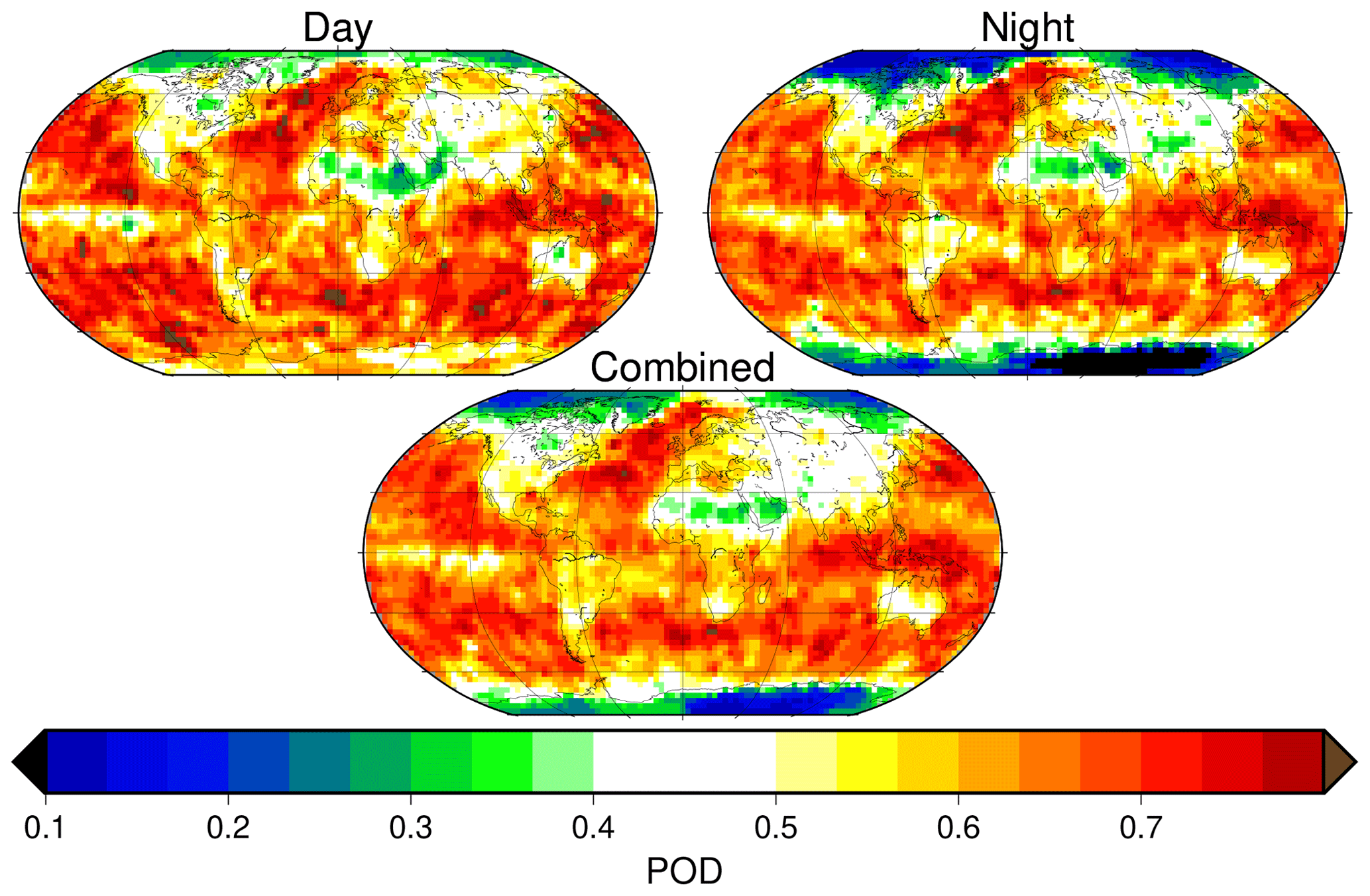
Figure 1Probability of detection of clouds having an optical depth between . The τc in the center of this interval, 0.225, is the global average of the smallest τc threshold where the CLARA-A2 cloud mask detects more clouds than it misses according to CALIOP (see text).
2.2 ISCCP-H
The ISCCP-H CDR (Young et al., 2018) is a recently released high-resolution version of the ISCCP CDR (Rossow and Schiffer, 1999) that starts in July 1983 and ends in June 2015 due to data availability at the time of this study. The ISCCP CDR comprises of geostationary and polar-orbiting satellites, where data from the geostationary satellites have precedence at low latitudes and midlatitudes (absolute latitude <55∘). The main improvement of ISCCP-H CDR is that it is on a higher-resolution spatial grid compared to its predecessor, and it covers a more extended period. Otherwise, the ISCCP-H CDR is quite similar to previous ISCCP versions. The CDR uses bispectral radiances, with one channel in the visible (0.6 µm) and one in the infrared (11 µm). Karlsson and Devasthale (2018) and Tzallas et al. (2019) describe this CDR at length.
2.3 The EC-Earth model
The EC-Earth climate model (Hazeleger et al., 2010, 2012) is an ESM with its atmospheric component based on the Integrated Forecast System (IFS) of the European Centre for Medium-Range Weather Forecasts (ECMWF). The version used for this study is 3.3, based on IFS cycle 36r4 and on a horizontal resolution of T255 with 91 vertical layers. The variant used in this study is the EC-Earth-Veg3 Atmospheric Model Intercomparison Project (AMIP) simulation with prescribed monthly sea surface temperatures and sea ice conditions to enable comparisons with atmospheric observations. The temporal range used to demonstrate the simulator covers 1982 to 2015 when compared only to the CLARA-A2 CDR and covers July 1983 to June 2015 when ISCCP-H is involved in the comparison. EC-Earth produces simulated ISCCP clouds at run time through the COSP. In terms of cloudiness, EC-Earth has no lower or upper limit to cloud optical thickness aside from numerical precision. Therefore, any satellite simulator should always produce less cloudiness than the direct model output.
Table 1The cloud variables produced by the simulator. The middle column specifies the separate categories available for each variable, and the third column indicates under which illumination conditions the variables are available.
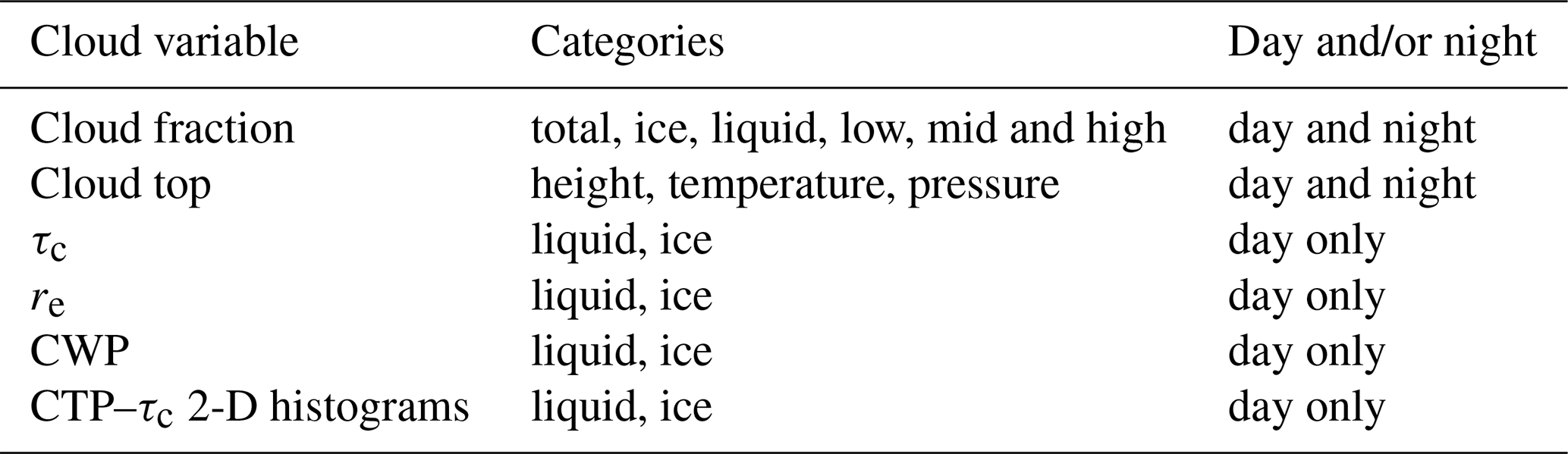
Table 1 lists the variables simulated by the CLARA simulator, and this section provides an overview of them. As briefly described in the introduction and detailed in Bodas-Salcedo et al. (2011) and Jakob and Klein (1999), the CLARA-A2 simulator relies on subcolumns within the climate model grid, as all the COSP simulators do, to simulate the observational dataset cloud variables. The subcolumns created in each model grid together produce the horizontal and vertical cloud structure that preserves the internal cloud overlap assumption of the host model. Each subcolumn has the same number of layers as the model, and each layer in a subcolumn is either completely cloudy or clear.
The next stage in the simulation is to map the average model layer in-cloud2 optical depth, water content, and effective radius, both liquid and ice phase, to the cloudy layers of each subcolumn. Every subcolumn is determined to be either cloud-free or cloudy, and the simulator performs cloud retrievals on each “cloudy” subcolumn, and these represent the column-integrated retrievals of CLARA-A2. Finally, the simulated cloud parameters are averaged to the climate model grid so that they are ready to be directly compared to observations. Table 1 provides an overview of the simulated variables included in this simulator. The CLARA-A2 satellite simulator can currently only be run in an offline mode, meaning that it relies on access to preprocessed model output files. Following is a short description of the simulated cloud retrieval simulation:
-
Cloud microphysics. The cloud microphysical retrievals τc, cloud particle effective radius (re), cloud water path (CWP), and cloud phase are simulated using the same method described in Eliasson et al. (2019), which very closely resembles the method described in Pincus et al. (2012). The dominant cloud water phase of the top optical depth of the cloud determines the simulated cloud water phase. The simulation of the effective radius, re, is calculated by comparing the top of the atmosphere reflectance, calculated by the adding–doubling technique, to lookup tables of reflectance versus cloud effective radius. The lookup tables for the effective radius simulation rely on the same microphysical model as the CLARA-A2 CDR (see details in Karlsson et al., 2017a). The simulated optical depth and cloud water path is the sum in the column. For consistency with observations, if a cloud parameter requires sunlight for its retrieval, it will only be simulated if the calculated solar zenith angle is less then 84∘. These include the cloud microphysical retrievals τc, re, CWP, and the cloud top pressure (CTP)–τc histograms.
-
Cloud top. The simulated CTP, cloud top height (CTH), and cloud top temperature are calculated by two methods depending on if the clouds are optically thick or not. If a subcolumn has a simulated cloud optical depth, τc≥5, it is considered opaque, and finding the cloud top is achieved by matching a calculated brightness temperature to the model temperature profile, i.e., precisely the same approach to simulate cloud top as used by the ISCCP simulator (Jakob and Klein, 1999).
However, acknowledging that accurately determining the cloud top of optically thin, i.e., semitransparent clouds, is more complicated than for opaque clouds (Håkansson et al., 2018), the CLARA simulator has a different method for simulating thin clouds. As a first step, the simulator finds the height that is one optical depth down from the top of the model cloud. This first step corresponds to how the MODIS simulator (Pincus et al., 2012) and Cloud_cci simulator (Eliasson et al., 2019) calculate the CTH. The CLARA-A2 simulator then offsets this height using the median error in CTH for semitransparent clouds in the CLARA-A2 CDR (Table 13 in SMHI, 2018). This approach emulates the real-world performance of the CLARA-A2 cloud top retrievals more closely for semitransparent clouds than treating all clouds as opaque. The offsets used are 257, −145, and −3336 m for low (CTP ≥ 680 hPa); middle (440 hPa ≤ CTP > 680 hPa); and high clouds (CTP < 440 hPa), respectively.
3.1 Simulating CLARA-A2 cloud masks
As mentioned in Sect. 1, the main feature of the CLARA-A2 simulator is a more sophisticated simulation of the observational dataset's cloud mask. It is possible to choose between one of the three methods of cloud mask simulation described below.
3.1.1 A globally static optical depth threshold
Method one is to simulate the cloud mask using one global minimum cloud optical depth value. Method one is also the classical approach used by the ISCCP, MODIS, MISR, and the Cloud_cci simulators. For the ISCCP, MODIS, and MISR simulators, this global limit is τc = 0.3 (Pincus et al., 2012); for the Cloud_cci simulator (Eliasson et al., 2019), it is 0.2. As mentioned earlier, the global average τc threshold for the CLARA-A2 CDR is 0.225, and thus the threshold used in method one of the CLARA-A2 simulator.
By the approach used in this method, all cloudy subcolumns with an optical thickness less than the global average τc limit are treated as being cloud free and all subcolumns above this threshold as cloudy. Since the threshold is a global average, this method does not consider the illumination conditions or the geographical location of the retrieval. The advantage of this approach is its robustness and simplicity. However, as mentioned in Sect. 2.1, this approach can lead to very misrepresentative cloud mask simulations in some geographical regions.
The cloud retrieval simulations in the COSP are only carried out during sunlit conditions. However, the next two approaches described below also simulate the cloud amount and also the cloud top retrievals during nighttime conditions. However, the variables re, τc, CWP, and the CTP–τc 2D histograms are only simulated during daytime conditions.
3.1.2 Gridded optical depth thresholds
The second method uses varying gridded optical depth thresholds. This method also relies on the robust and straightforward approach of reclassifying subcolumns with a small optical depth as cloud free, while keeping those above this threshold cloudy. However, this method takes into account that the τc threshold, or cloud detection limit, varies geographically and depends on the solar illumination. This method relies on the gridded data used in Fig. 12 in Karlsson and Håkansson (2018) that shows the smallest τc threshold where the CLARA-A2 cloud mask detects more clouds than it misses (see Sect. 2.1).
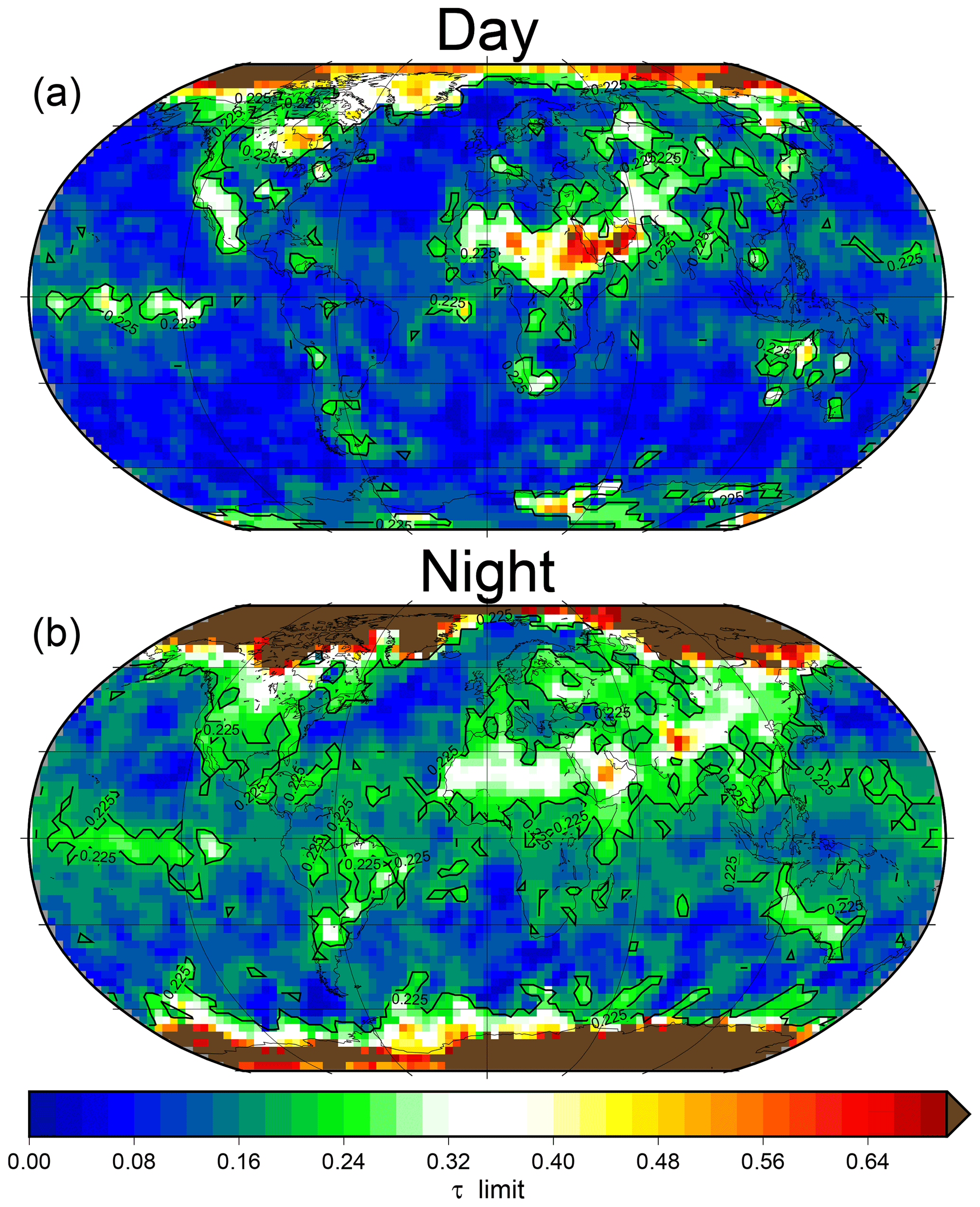
Figure 2The gridded cloud detection limit, i.e., the smallest τc threshold where the CLARA-A2 cloud mask detects more clouds than it misses according to CALIOP for sunlit (a) and nighttime (b) conditions. For reference, the global average τc threshold equal to 0.225 is shown as contour lines. These results are based on the results from the Karlsson and Håkansson (2018) study.
Figure 2 shows the detection limits used in the simulator according to this method. As shown by the figure, the τc threshold varies quite strongly regionally and also depends on if the CLARA-A2 cloud mask can make use of solar channels or not. The global average τc threshold, included for reference in the figure, clearly shows that during sunlit conditions the cloud mask is much more sensitive to thin clouds than a global average value of τc=0.225 suggests.
During sunlit conditions, the regions with the least cloud sensitivity are over the Arctic, the desert regions of the Sahara and Arabia and as a large patch in the central Pacific. During nighttime conditions, especially over the oceans, the cloud mask is generally less sensitive and is particularly degraded in the ice-covered regions. However, there is an improvement in cloud sensitivity in some regions during nighttime conditions. For instance, in the desert regions of northern Africa and the Arabian Peninsula, as well as the worst-performing areas in the central Pacific, the cloud mask is somewhat surprisingly better than when these regions are sunlit. Karlsson et al. (2017a) and Karlsson and Håkansson (2018) provide a more in-depth validation study on CLARA-A2.
Their results demonstrate that using two sets of gridded detection limits gives a more realistic cloud mask, one for sunlit and one for nighttime conditions. Method two is more realistic than the global static minimum optical depth approach of method one (Sect. 3.1.1). However, the authors of this paper advocate the further-improved simulated cloud mask, based on the use of PODs described in the next section, that also emulates some of the expected variability in cloud detection over a range of cloud optical depths.
3.1.3 Probability of cloud detection
The third method is an approach to simulate the CLARA-A2 cloud mask using the PODs, provided on a roughly 300 km grid, as a function of the cloud's optical thickness. These POD, discussed in Sect. 2.1, are treated as the likelihood that the cloud mask would detect the model cloud given its optical thickness, geographical location, and whether or not it is sunlit.
The simulator uses computer-generated random numbers for comparison to the gridded POD value found in a lookup table, where one set of optical-depth-dependent PODs is for sunlit and another is for nighttime conditions. The simulator assigns a random number between 0–1 to each subcolumn at the initiation. After simulating the τc, the column-integrated τc, latitude and longitude are used to find the POD value from the lookup table for comparison. A subcolumn is cloudy only if its assigned random number is less than the POD. Therefore, if the probability of detection of a cloud with a specific optical depth is 0.05, even though it is very transparent, there is still a 5 % chance the subcolumn will be considered cloudy. Conversely, regardless of how optically thick a cloud is in a subcolumn, there is a nonzero chance this subcolumn will not be flagged as cloudy, and hence not included in any further cloud simulations.
Table 2The probability of cloud detection for the CLARA-A2 cloud mask separated by intervals of CALIOP cloud optical thickness. This table shows the regional averages based on the POD values used in the simulator of large geographical regions. Note that the simulator makes use of gridded POD values on a 300 km equal-area grid (see Fig. 3) and not the POD regional averages provided here for reference. The polar region here refers to latitudes >75∘ (north and south). The values apply to daytime (nighttime) conditions. These results are based on the results from the Karlsson and Håkansson (2018) study.
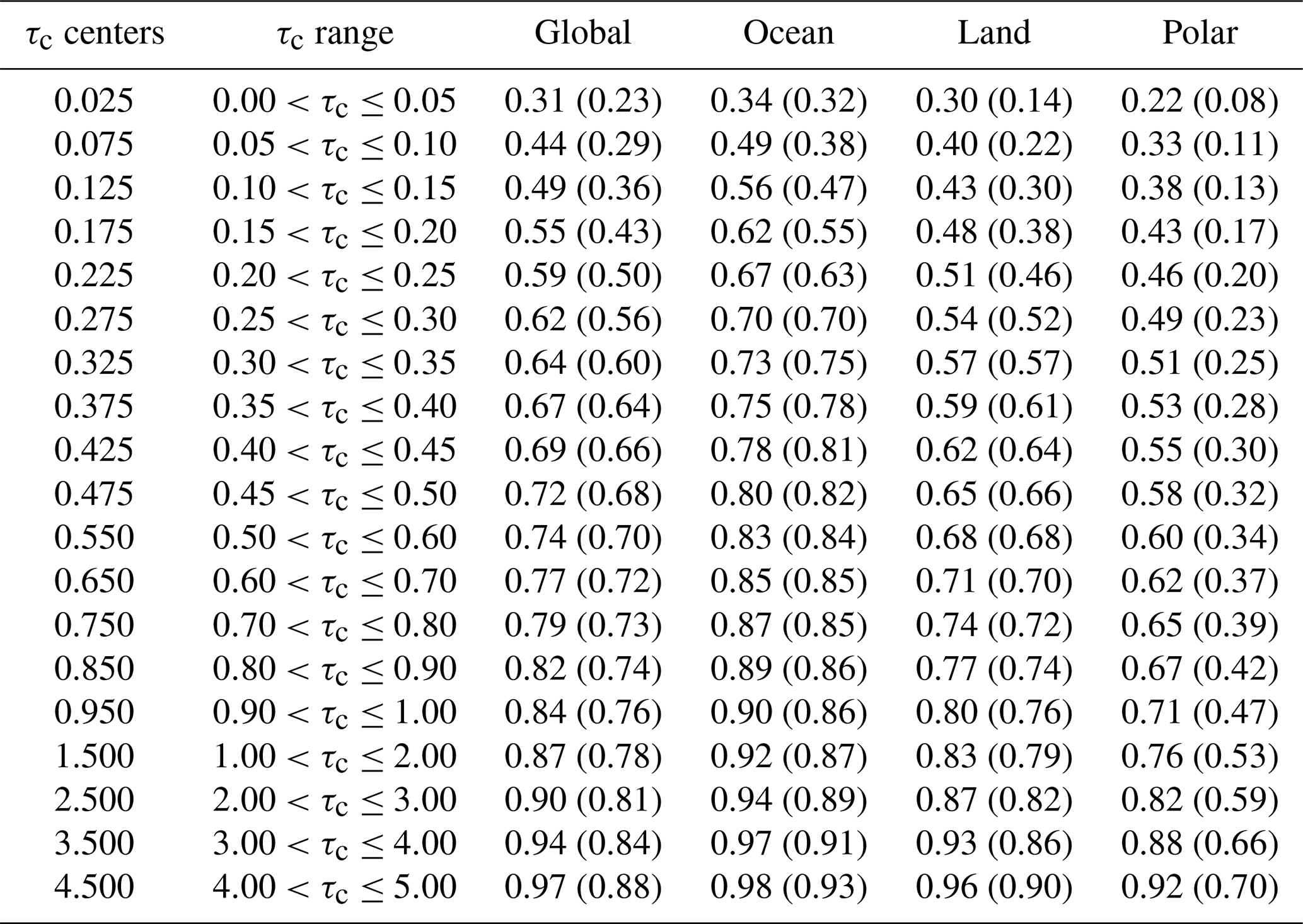
The lookup table of gridded POD used by the simulator contains separate values for each of the τc intervals listed in Table 2. The primary purpose of Table 2 is to list all of the POD intervals used to simulate the cloud mask, but it also provides a summary of average POD separated into global, ocean, land outside the polar regions, and the polar regions during sunlit conditions (nighttime in parenthesis). As is entirely intuitive, the POD increases for optically thicker clouds for all regions, and, in general, the cloud mask is more sensitive to clouds over ice-free oceans. Additionally, nowhere, and not even for the thickest clouds, does the POD reach 1. Karlsson and Håkansson (2018) discuss this apparent paradox at length, and here is a summary:
-
Thick clouds are likely undetectable if they have the same temperature as the underlying surface during nighttime conditions when solar reflectivity measurements are not available.
-
Colocation errors between CALIOP and AVHRR can cause a mismatch between the datasets. Some colocation error is unavoidable due to the maximum time difference of 3 min and because sometimes the geolocation data for AVHRR itself may not be sufficiently accurate.
-
Even if the data are ideally colocated, the FOVs of the measurements most likely differ somewhat due to how the GAC footprint is made (see Fig. 1 in Karlsson and Håkansson, 2018, and Sect. 2.1 here).
In fairness, only the first point directly has to do with the skill of the CLARA-A2 cloud mask, and thus it should be simulated. The next two points have to do with imperfections in the validation process, and therefore they should not be simulated. Unfortunately, currently, all three points reduce the POD. In the future, it could make sense to estimate and take into account the impact of all three of these considerations in the simulator.
On the other hand, results from Table 2 indicate that the impact of points two and three may not be that strong after all. Over global oceans during the daytime, i.e., the areas with the highest POD values, the detection rate for the most optically thick clouds is 98 %. Therefore, on average, the combined error from points two and three is probably less than 2 %. However, in some oceanic regions where relatively thick inhomogeneous clouds are prevalent, such as the stratocumulus-dominated regions off the west coast of South America and southern Africa, POD values are slightly below 0.9, hence the impact of points two and three may not be negligible in these regions.
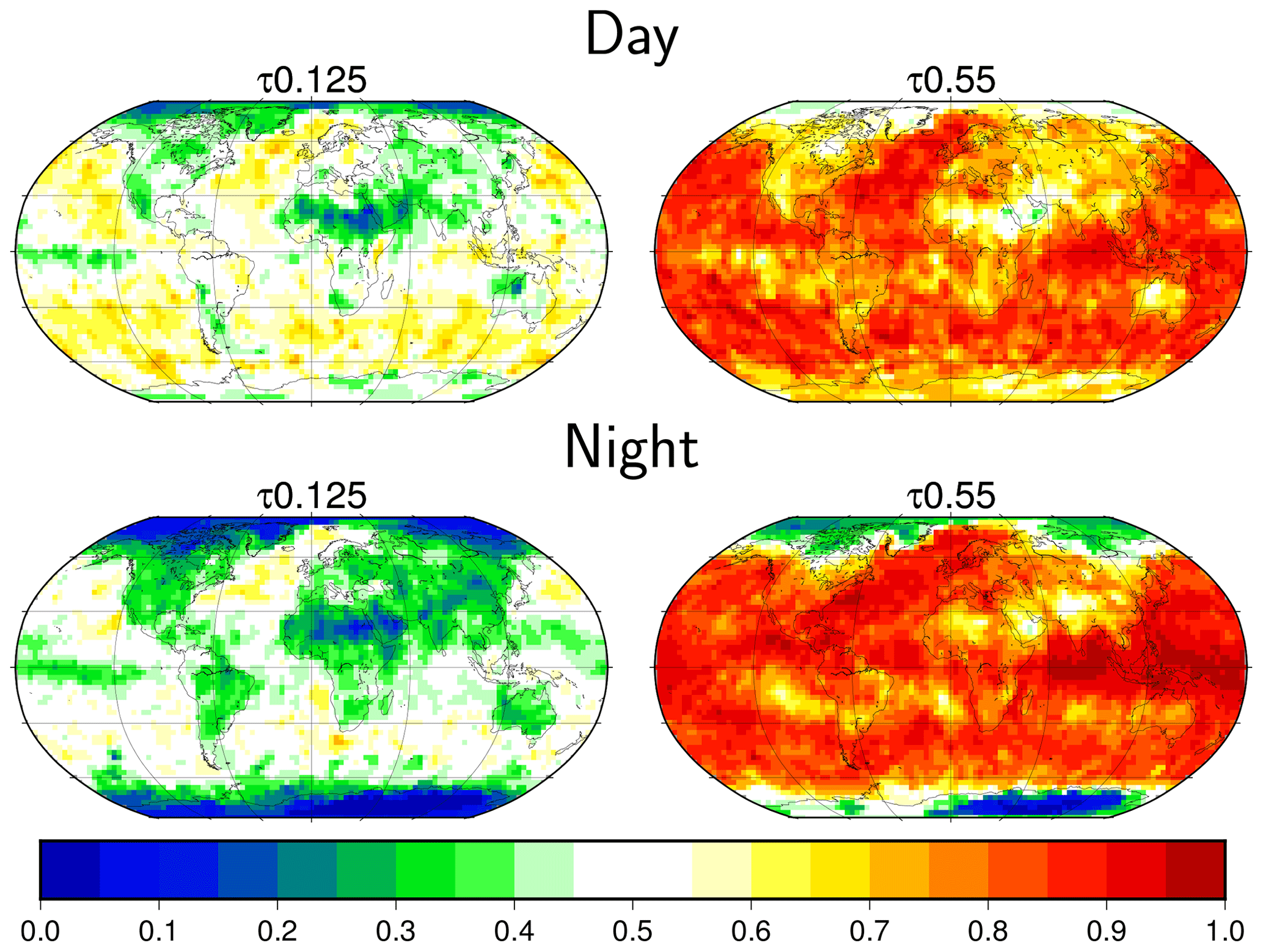
Figure 3The probability of detection at two τc intervals centered at 0.125 and 0.55 for day and night conditions. These results are based on the results from the Karlsson and Håkansson (2018) study.
To illustrate the global distribution of POD, Fig. 3 contrasts two τc intervals used by the simulator. Clouds that fall in the interval centered at τc=0.125, which are translucent clouds at only half the global average τc limit (see Sect. 3.1.1), generally have a low POD. The POD is particularly low in this interval over land and during nighttime conditions. However, take notice that, especially over ocean areas and especially during sunlit hours, there is at least a 50 % POD despite the clouds being so thin.
For clouds centered at τc=0.55, which is about twice the global average detection limit, the PODs are predictably quite high in general. However, again, this is not true globally. Even though the clouds are relatively thick, in areas such as northern Africa, the Arabian peninsula, and the polar regions, the POD is only around 50 %. Another striking feature is that for these semitransparent clouds, the POD over nearly all regions, except the poles, are higher for cloud retrievals made during nighttime conditions. This result is demonstrated further in Fig. 4. Outside the polar regions, clouds in the τc intervals from 0.2 to 0.6 have a higher POD during nighttime conditions overall (especially in the tropics), whereas for clouds thinner or thicker than this interval, the daytime cloud masks have better success.
The fact that this slightly improved detectability at night for clouds in the τc range 0.5–1.0 is a robust feature is supported by intercomparisons made between CLARA-A2 and other AVHRR-based datasets (e.g., Karlsson et al., 2017a; Karlsson and Devasthale, 2018). They found (although not explicitly reported in the papers) the same behavior for results from PATMOS-x and Cloud-cci compared to CALIOP observations. Whether to interpret this as an indeed improved nighttime detectability for AVHRR-based methods or something caused by the CALIOP observation reference (e.g., enhanced daytime problems due to lower signal-to-noise ratios) is currently unclear. However, this feature is not critical to the CLARA-A2 simulator, but it merits a more in-depth investigation in the future.

Figure 4The difference in the POD of the cloud mask during sunlit and nighttime conditions for selected cloud optical depth intervals. These results are based on the results from the Karlsson and Håkansson (2018) study.
3.2 The choice of the simulated cloud mask
In this section, we refer to Figs. 5 and 6 to illustrate how the choice of cloud mask simulation method affects the comparison of cloud cover of EC-Earth to CLARA-A2. The results are separated into seasons here since it is essential to understand the seasonal impact of choosing one method over another. Figures 5a and 6a show the cloud cover according to CLARA-A2 for 1982–2015 during Southern Hemisphere summers and the Northern Hemisphere summers, respectively. EC-Earth minus CLARA-A2 based on the first method (Sect. 3.1.1) is panel (b), based on the second method (Sect. 3.1.2) is panel (c), and based on the third method (Sect. 3.1.3) is panel (d). Panel (e) shows the difference between the simulated cloud mask based on method one, a global static τc threshold, and method three, based on POD thresholds (first method minus the third method).

Figure 5Total cloud cover during the DJF seasons of 1982–2015. This figure shows a comparison of EC-Earth to CLARA-A2 using three different methods of cloud mask simulation. The reference figure at the top (a) is the cloud fraction from CLARA-A2. Panel (b) shows the simulated observations using method one, based on a global static τc limit minus CLARA-A2. Panel (c) shows the same comparison using method two, based on gridded τc limits, and (d) shows the same using method three, based on POD. Panel (e) shows the difference between the simulated CF based on method one minus method three. See Sect. 3.2 for a wider description of the figure.
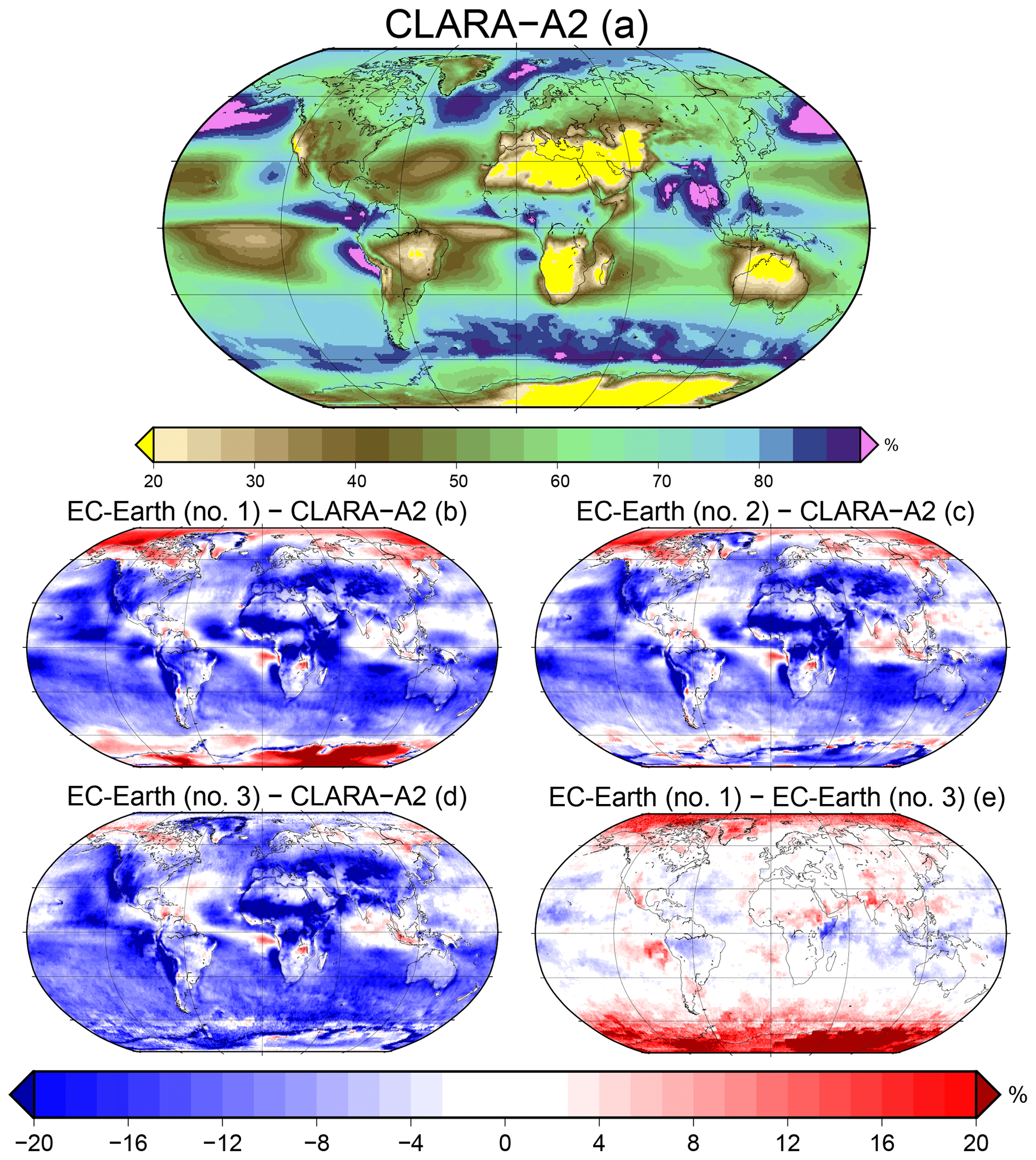
Figure 6Total cloud cover during the JJA seasons of 1982–2015. See the description in Fig. 5 for a description of the layout in this figure.
Globally, the overall impression is that EC-Earth underestimates cloud fraction. In most regions of the world, within a few percent, this is the conclusion one would reach regardless of which of the three methods was used to simulate the CLARA-A2 cloud mask. However, as described in Sect. 2.1, the CLARA-A2 CDR is systematically and substantially less skillful under certain conditions than on average.
As discussed in Sect. 2.2, CLARA-A2 is skillful at detecting clouds in the polar regions during sunlit conditions but not so during the polar winter. For this reason, the apparent overestimation of clouds in these regions by EC-Earth (Figs. 5b and 6b) is likely strongly exaggerated. Without prior knowledge of the retrieval difficulties in cold dark locations, i.e., when only passive infrared channels are available, if using method one to simulate clouds, one could erroneously conclude that EC-Earth places too many clouds in polar regions. This problem is especially salient during winter months, but it also has a considerable impact on cumulative averages over these regions. Therefore cloud mask simulations based on method one are notably unsuitable in the polar regions and, to a lesser extent, desert areas.
However, and what is the main point of this innovation, if one uses the second or third method to simulate clouds, the apparent bias in cloudiness in these regions is mostly removed in the problematic regions. The second and third methods do a much better job at reproducing the limitations of cloud datasets than the first method, and the size of the difference between method three and method one is substantial and seasonally dependent in the problematic regions (Figs. 5e and 6e).
Notice also from Figs. 5c and d and 6c and d that the second and third methods produce similar results, and hence both do well in this regard. However, there are some subtle differences. One is that during the Northern Hemisphere summer months, a model validation based on the second method leads to the conclusion that EC-Earth overestimates clouds in the Arctic, yet if the comparison were made based on the third method, one would conclude that only a slight overestimation occurs here.
The third method gives the most accurate description of the cloud detection limitations since it describes the likelihood of detecting or missing clouds over the full range of cloud optical thicknesses for day and night conditions. Also, method three can emulate the nonzero probability that even thick clouds might be undetectable under certain conditions. This approach better describes the skill of the cloud retrievals of a satellite dataset than using gridded static values of τmin in method two, and especially instead of using a single global τmin value used by method one. Overall, therefore, the recommendation is to choose method three to simulate the cloud mask.
However, the advantage of tying statistics to geographical regions may also be a weakness in some situations. If a model's cloud distribution is systematically misplaced, the model clouds may be subject to (potentially) other PODs than what they should have been in the CLARA-A2 simulator. The consequences here should not be large, except for the extreme cases when a model places clouds over ice- and snow-covered areas in the polar night (with very low PODs) instead of over adjacent ice-free ocean areas (with very high PODs). Another factor to consider is that the underlying statistics used in methods two and three derive from colocations from the period 2006–2015 (see Sect. 2.2). Therefore, in some regions, such as where there is marginal ice, the conditions for cloud detection may have changed appreciably from those during the validation period, for instance, due to a changing climate, rendering the statistics less representative than in more climatically stable regions.
4.1 Average cloudiness during summer months
Karlsson et al. (2017a) asserted, and the POD maps in Fig. 4 suggest, that the CLARA-A2 CDR is reasonably skillful at detecting clouds in the Arctic during sunlit conditions. Therefore, to demonstrate the utility of the CLARA-A2 simulator, we assessed the cloud cover in these conditions over the full length of the datasets. We added the ISCCP-H CDR (Young et al., 2018) to the comparison since it is an equivalent CDR with a well-established satellite simulator used in many previous model studies (e.g., Webb et al., 2001; Norris et al., 2016; Terai et al., 2016; Tan et al., 2018). However, Karlsson and Devasthale (2018) found the cloud cover of ISCCP-H too low in the polar summer and early autumn.
The cloudiness from ISCCP-H should be compared to the simulated cloudiness using the ISCCP simulator (Jakob and Klein, 1999), and the cloudiness, according to CLARA-A2, is compared to the CLARA-A2 simulator. Figure 7 shows the average cloudiness in Arctic summer months according to CLARA-A2 (Fig. 7a) and ISCCP-H (Fig. 7b). Figure 7c and d show assessments of the overall cloudiness during the Arctic summer by EC-Earth using the simulated CLARA-A2 and simulated ISCCP-H, respectively. As mentioned in Sect. 3.1.1, the simulated cloud mask for ISCCP-H uses a global τc threshold (τc=0.3) for the simulated cloud mask (method one, different threshold), and the CLARA-A2 simulator uses the POD-based approach for the simulated cloud mask (method three). The two satellite datasets and the climate model are limited to July 1983 to June 2015 to match the availability of the ISCCP-H period to date.
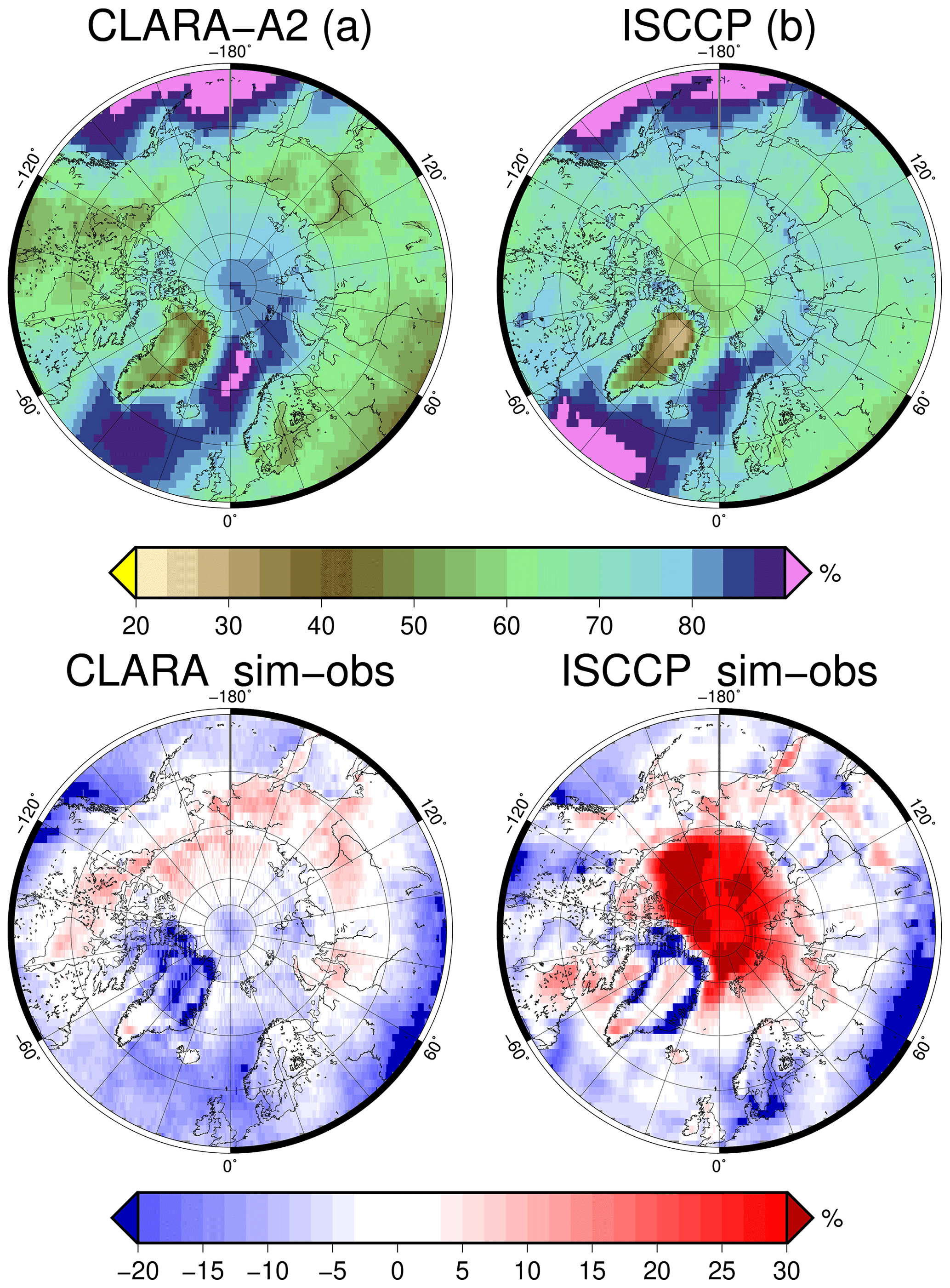
Figure 7The total cloud fraction in the Arctic summer. The top row contains the observations from two equivalent CDRs, CLARA-A2 (a) and ISCCP-H (b). The bottom row contains the difference between the simulated CDR minus the CDR for CLARA-A2 (c) and ISCCP-H (d). The period is July 1983 to June 2015.
Figure 7 demonstrates that using simulators that do not take the variable skill of the cloud mask into account, such as the ISCCP simulator, could easily lead to false conclusions about EC-Earth cloud cover in the Arctic summer. Compared to the ISCCP-H observations, the simulated ISCCP-H observations indicate that EC-Earth has a robust positive cloud bias in the Arctic of more than 30 %. However, CLARA-A2, shown to have a high skill in the polar summer (see Fig. 5b in Karlsson et al., 2017a), indicates that EC-Earth underpredicts the cloudiness in large parts of this region by more than 10 %.
The substantial differences between the simulated ISCCP-H and CLARA-A2 are mainly due to the ISCCP simulator being too sensitive to thin clouds here. As shown in Fig. 2, during daytime conditions in the Arctic, a more appropriate daytime τc limit would be around 0.5 or more, which is higher than the global average of 0.3 assumed by the ISCCP simulator. Therefore, in the Arctic summer, the ISCCP simulator retrieves clouds in between these cloud optical thicknesses that the CLARA-A2 simulator, and most likely the observations, do not. As a consequence, anyone assessing cloudiness in the Arctic will reach the opposite conclusion using the CLARA-A2 CDR and simulator compared to the ISCCP-H counterpart.
Overall, based on CLARA-A2 as the reference, EC-Earth has a smaller average cloud fraction over most of the region between 50–90∘ N during the summer months. The difference is more substantial over ocean areas than over land, with the largest underrepresentation of cloudiness at these latitudes over the North Atlantic and following the Gulf Stream north of Norway. However, globally, the most considerable negative cloud biases between the model and observations are in the tropics and subtropics (see Fig. 6).
4.2 Trends in cloudiness
The CLARA-A2 CDR is particularly suitable for cloud trend analysis in the Arctic summer due to its length and high cloud detection skills there (Karlsson and Devasthale, 2018). Here is an assessment of the cloud trends from the months that have enough sunlight, i.e., where the solar zenith angle is less than 84∘ in the Arctic, above 70∘ N for CLARA-A2 and EC-Earth. These trends are based on the linear regression of cloudiness from all data in 1982–2015 and expressed here as the absolute change in cloudiness (% per decade).

Figure 8The average trend in cloudiness over the entire record (% per decade) in the Arctic from the illuminated months of April to August according to CLARA-A2. Negative trends correspond to an average decrease in cloudiness over time. The trends are from all months in the period 1982–2015.
Figure 8 shows the distribution of cloudiness trends, according to CLARA-A2. From this figure, some distinct patterns emerge; in the spring months, there is an increase in cloudiness by more than 5 % in large parts of the Arctic and upwards of 10 % north of Novaya Zemlya, and in the summer to Autumn months the Arctic is dominated by a decrease in cloudiness. The increase in cloudiness reaffirms observations previously reported in Kapsch et al. (2013, 2019). Kapsch et al. (2013) asserted that the increase in cloudiness is likely due to an increased intrusion of water vapor into these regions during the spring months. The most substantial decrease in cloudiness seen in July and August is in the Beaufort Sea, and especially the Lincoln Sea, north of the Canadian Arctic Archipelago and Greenland. However, it is outside the scope of this study, where the primary purpose is to describe the CLARA-A2 simulator, to further assess the possible reasons for the changing cloudiness seen in these observations.

Figure 9As for Fig. 8 but for the EC-Earth climate model.
Figure 9 shows the average change in cloudiness from EC-Earth, over the same period used in Fig. 8, using method three to simulate the cloud mask. The cloud trends in the model differ from the observations. In particular, the trends are much smaller and differently distributed (except in May) than the observations indicate. However, there are some critical limiting factors to consider for this model evaluation.
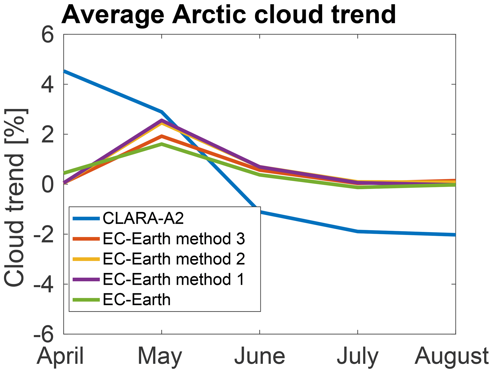
Figure 10The average decadal cloudiness trend in the Arctic from the illuminated months of April to August only over the ocean (ice-free or ice-covered). The figure shows the reference dataset, CLARA-A2, the CLARA-A2 simulator, one line for each method, and the total cloud cover from the EC-Earth model without using any simulator. The trends are from all months in the period 1982–2015.
EC-Earth is represented here by only one model run, and, although it employs prescribed sea surface temperatures and sea ice extent, the model atmosphere is free to meander. In order to assess if the model cloud trends agree with the observations, ideally several ensemble model runs are required to find a general trend to assess whether or not the natural variability produced by the model is accurate (Koenigk et al., 2019).
Figure 10 illustrates how the choice of cloud mask simulation affects the model cloud trend. Fig. 10 shows the average cloudiness trends for the same conditions, aside from excluding land areas, as in Fig. 8, for CLARA-A2, the three methods of simulated CLARA-A2 cloud mask from the EC-Earth atmosphere, and the total cloudiness directly from EC-Earth without any simulator.
Figure 10 illustrates that regardless of which method is used to simulate cloudiness, or even using no simulator at all, the simulators do not appear to alter the cloud trends in the Arctic summer. These results may indicate that the clouds in the model are not changing the average range and distribution of optical thicknesses over time, even if the actual cloud amounts may change.
In summary, no definitive conclusions on model cloud trends in the Arctic can be drawn here for the reasons listed above, and a more thorough examination of whether or not EC-Earth reproduces realistic cloud trends is also outside the scope of this study. Although the choice of method does not appear at first glance to impact the model cloudiness trends, it still makes sense, in this case, to use method three to simulate clouds, since it more closely reflects the skill of the CLARA-A2 dataset.
This article describes a satellite simulator designed to enable comparisons between climate models and the CLARA-A2 CDR. Typically, satellite simulators simulate the satellite-retrieved cloud fraction using one global cloud optical depth threshold to remove thin model clouds that are presumed undetectable by the instruments used to generate the CDR. There are more factors to consider that influence the ability to retrieve thin clouds. These include the following:
-
the optical thickness of the cloud,
-
how illuminated the clouds are,
-
the underlying surface properties, and
-
the temperature difference between the cloud and the surface.
In this paper, we show that using one optical depth threshold for all conditions to emulate cloud sensitivity, denoted here as method one, is inappropriate since the cloud detection skill of satellite retrievals may vary considerably. Method one is the method used in the COSP simulators on which many previous studies have relied. Therefore, to avoid the most substantial uncertainties, many studies are limited to between ±60∘ latitude. There is a need for a more realistic simulated cloud mask that better reflects the actual cloud detection ability of the CDR. We, therefore, propose two other methods that are both based on validations of the CLARA-A2 CDR using colocated cloud retrievals from CALIOP by Karlsson and Håkansson (2018).
Method two uses two maps of cloud detection thresholds on a 300 km grid, one for day and one for night conditions. These thresholds refer to the smallest cloud optical depth where there is a 50 % success rate in detecting clouds. Method three, the recommended approach to simulating the cloud mask, is based on the POD of clouds depending on their τc. Instead of using a τc threshold to determine whether or not a model cloud would have been detected, with this approach any model cloud could potentially be detected or missed. Maps of POD valid for separate optical depth ranges (see Table 2) are used together with a random number generated at run time for every model subcolumn to determine cloudiness. These are also provided on a 300 km grid and separated by day and night.
The main improvements for methods two and three are the following:
-
The cloud sensitivity generally increases, i.e., with lower cloud optical thresholds (method two) and higher PODs (method three), in areas where the cloud retrievals are relatively straightforward, such as over midlatitude oceans.
-
More suitable, higher optical depth thresholds (method two) and lower PODs (method three) apply in areas and conditions where cloud retrievals are notoriously tricky.
-
Method three indirectly takes into account that retrievals in some regions are more likely than others to miss thick clouds. This situation is common in cold regions where thick clouds may be inseparable from cold, snow-covered surfaces and also in regions with an abundance of broken and small-scale cumulus clouds such as the atmospheric subsidence regions over the ocean.
Compared to method one, methods two and three allow for analyses to be carried out at high latitudes and during nighttime conditions. Although the most significant improvements are at high latitudes, these new methods also account for the modestly improved cloud detection of CLARA-A2 over the global oceans compared to, in particular, desert areas. Therefore, with these methods, model studies may also be improved for regions outside the polar regions.
This paper illustrates that these new approaches to cloud mask simulation bring the model and observations much closer to each other compared to using a fixed optical depth threshold globally to filter out clouds. They allow for a more realistic model to satellite comparison, and thus reduces the likelihood that incorrect conclusions from model assessments are reached simply due to cloud simulations not correctly representing the cloud retrievals of the CDR. Although methods two and three both significantly improve cloud mask simulations, method three, using the POD approach, is better since it realistically mimics the performance of the cloud mask of the CLARA-A2 CDR over the full range of cloud optical thicknesses.
The overall cloudiness in the Arctic during summer months from 1984–2014 is used to demonstrate the usefulness of the simulator and the new approach to cloud mask simulation. The ISCCP-H CDR here complemented the comparison as a second independent satellite dataset. Therefore, EC-Earth was assessed using both the ISCCP and CLARA-A2 simulators and compared to the corresponding CDR. This comparison shows that EC-Earth seems to produce too few clouds in and around the Arctic compared to CLARA-A2.
However, despite the ISCCP-H CDR having more clouds than CLARA-A2 in the Arctic summer months, compared to ISCCP-H and using the ISCCP simulator, the assessment on EC-Earth cloudiness would lead to quite the opposite conclusion in some regions in the Arctic. The simulated ISCCP cloudiness is substantially higher than the ISCCP observations. This overrepresentation of clouds is mostly due to the ISCCP simulator using a global optical depth threshold that, in the Arctic, is too generous. This example demonstrates the advantage of using the CLARA-A2 approach to cloud mask simulation compared to the traditional approach used by the ISCCP simulator and others. Although only demonstrated in the Arctic summer in this paper, the POD approach, method 3, is also the most appropriate globally.
In terms of trends in overall cloudiness in the Arctic for all months with sunlit conditions from 1982–2015, the observations from CLARA-A2 show a sharp increase in cloudiness over the years, especially in the ocean areas north of western Russia, in the spring months of April and May. In the summer and early autumn months, there is a large area of decreasing cloudiness in the seas just north of Canada and Greenland. Although only based on one model run, and therefore clear statements about cloud trends in the model cannot be made, one can deduce that the average cloudiness trends from the model are very similar using any simulator method, or no simulator at all.
In summary, the authors advocate an approach to cloud mask simulation based on the probability of detection of clouds depending on their optical depth, location, and illumination. This study suggests that evaluations of climate model simulations of cloudiness parameters would benefit substantially from using more advanced satellite simulators, which, in a better way than today, accounts for weaknesses and strengths of satellite retrievals.
The CLARA-A2 CDR can be downloaded from https://wui.cmsaf.eu (last access: 30 July 2019, Karlsson et al., 2017d). Data from the EC-Earth global climate model can be obtained from http://catalogue.ceda.ac.uk/uuid/526ec947ec2d4467b128749e9fe46f1a (EC Earth consortium, 2017). The ISCCP-H products and other ISCCP products are available from https://data.nodc.noaa.gov/cgi-bin/iso?id=gov.noaa.ncdc:C00956 (last access: 16 January 2020, Rossow et al., 2016).
The CLARA-A2 simulator code is available at https://github.com/SatelliteSimulators/AVHRR_based_satellite_simulators (Eliasson, 2019).
SE is the principal author. KGK provided data and expertise on the CLARA-A2 CDR. UW provided expertise from the climate model perspective. All three authors were instrumental in planning the structure of and main points of the article.
The authors declare that they have no conflict of interest.
This work was partly funded by EUMETSAT in cooperation with the national meteorological institutes of Germany, Sweden, Finland, the Netherlands, Belgium, Switzerland and the United Kingdom.
This research has been supported by the Swedish National Space Agency (grant no. 121/14).
This paper was edited by Klaus Gierens and reviewed by two anonymous referees.
Bodas-Salcedo, A., Webb, M. J., Bony, S., Chepfer, H., Dufresne, J.-L., Klein, S. A., Zhang, Y., Marchand, R., Haynes, J. M., Pincus, R., and John, V. O.: COSP: satellite simulation software for model assessment, B. Am. Meteorol. Soc., 92, 1023–1043, https://doi.org/10.1175/2011BAMS2856.1, 2011. a, b
Bugliaro, L., Zinner, T., Keil, C., Mayer, B., Hollmann, R., Reuter, M., and Thomas, W.: Validation of cloud property retrievals with simulated satellite radiances: a case study for SEVIRI, Atmos. Chem. Phys., 11, 5603–5624, https://doi.org/10.5194/acp-11-5603-2011, 2011. a
Dybbroe, A., Karlsson, K.-G., and Thoss, A.: NWCSAF AVHRR cloud detection and analysis using dynamic thresholds and radiative modelling – Part I: Algorithm description, J. Appl. Meteorol., 44, 39–54, 2005. a
EC Earth consortium: WCRP CMIP5: The EC-EARTH Consortium EC-EARTH model output collection, available at: http://catalogue.ceda.ac.uk/uuid/526ec947ec2d4467b128749e9fe46f1a (last access: 16 January 2020), 2017. a
Eliasson, S.: CLARA-A2 satellite simulator, https://doi.org/10.5281/zenodo.3577506, available at: https://github.com/SatelliteSimulators/AVHRR_based_satellite_simulators (last access: 22 January 2020), 2019. a
Eliasson, S., Buehler, S. A., Milz, M., Eriksson, P., and John, V. O.: Assessing observed and modelled spatial distributions of ice water path using satellite data, Atmos. Chem. Phys., 11, 375–391, https://doi.org/10.5194/acp-11-375-2011, 2011. a
Eliasson, S., Karlsson, K. G., van Meijgaard, E., Meirink, J. F., Stengel, M., and Willén, U.: The Cloud_cci simulator v1.0 for the Cloud_cci climate data record and its application to a global and a regional climate model, Geosci. Model Dev., 12, 829–847, https://doi.org/10.5194/gmd-12-829-2019, 2019. a, b, c, d, e
Håkansson, N., Adok, C., Thoss, A., Scheirer, R., and Hörnquist, S.: Neural network cloud top pressure and height for MODIS, Atmos. Meas. Tech., 11, 3177–3196, https://doi.org/10.5194/amt-11-3177-2018, 2018. a
Hazeleger, W., Severijns, C., Semmler, T., Ştefănescu, S., Yang, S., Wang, X., Wyser, K., Dutra, E., Baldasano, J. M., Bintanja, R., Bougeault, P., Caballero, R., Ekman, A. M. L., Christensen, J. H., van den Hurk, B., Jimenez, P., Jones, C., Kållberg, P., Koenigk, T., McGrath, R., Miranda, P., van Noije, T., Palmer, T., Parodi, J. A., Schmith, T., Selten, F., Storelvmo, T., Sterl, A., Tapamo, H., Vancoppenolle, M., Viterbo, P., and Willén, U.: EC-Earth, B. Am. Meteorol. Soc., 91, 1357–1364, https://doi.org/10.1175/2010BAMS2877.1, 2010. a, b
Hazeleger, W., Wang, X., Severijns, C., Stefanescu, S., Bintanja, R., Sterl, A., Wyser, K., Semmler, T., Yang, S., van den Hurk, B., van der Linden, T. v. E.-C., and van der Wiel, K.: EC-Earth V2: description and validation of a new seamless Earth system prediction model, Clim. Dynam., 39, 2611–2629, https://doi.org/10.1007/s00382-011-1228-5, 2012. a
Heidinger, A. K., Straka, W. C., Molling, C. C., Sullivan, J. T., and Wu, X. Q.: Deriving an inter-sensor consistent calibration for the AVHRR solar reflectance data record, Int. J. Remote Sens., 31, 6493–6517, https://doi.org/10.1080/01431161.2010.496472, 2010. a
Heidinger, A. K., Foster, M. J., Walther, A., and Zhao, X.: The Pathfinder Atmospheres-Extended AVHRR Climate Dataset, B. Am. Meteorol. Soc., 95, 909–922, https://doi.org/10.1175/BAMS-D-12-00246.1, 2014. a
IPCC: Clouds and Aerosols, p. 571–658, Cambridge University Press, https://doi.org/10.1017/CBO9781107415324.016, 2014. a
Jakob, C. and Klein, S. A.: The role of vertically varying cloud fraction in the parametrization of microphysical processes in the ECMWF model, Q. J. Roy. Meteorol. Soc., 125, 941–965, https://doi.org/10.1002/qj.49712555510, 1999. a, b, c, d, e
Kapsch, M.-L., Graversen, R. G., and Tjernström, M.: Springtime atmospheric energy transport and the control of Arctic summer sea-ice extent, Nat. Clim. Change, 3, 744–748, https://doi.org/10.1038/nclimate1884, 2013. a, b
Kapsch, M.-L., Skific, N., Graversen, R. G., Tjernström, M., and Francis, J. A.: Summers with low Arctic sea ice linked to persistence of spring atmospheric circulation patterns, Clim. Dynam., 52, 2497–2512, https://doi.org/10.1007/s00382-018-4279-z, 2019. a
Karlsson, K.-G. and Devasthale, A.: Inter-Comparison and Evaluation of the Four Longest Satellite-Derived Cloud Climate Data Records: CLARA-A2, ESA Cloud CCI V3, ISCCP-HGM, and PATMOS-x, Remote Sens., 10, 1–27, https://doi.org/10.3390/rs10101567, 2018. a, b, c, d
Karlsson, K.-G. and Håkansson, N.: Characterization of AVHRR global cloud detection sensitivity based on CALIPSO-CALIOP cloud optical thickness information: demonstration of results based on the CM SAF CLARA-A2 climate data record, Atmos. Meas. Tech., 11, 633–649, https://doi.org/10.5194/amt-11-633-2018, 2018. a, b, c, d, e, f, g, h, i, j, k, l, m, n, o, p, q
Karlsson, K.-G., Riihelä, A., Müller, R., Meirink, J. F., Sedlar, J., Stengel, M., Lockhoff, M., Trentmann, J., Kaspar, F., Hollmann, R., and Wolters, E.: CLARA-A1: a cloud, albedo, and radiation dataset from 28 yr of global AVHRR data, Atmos. Chem. Phys., 13, 5351–5367, https://doi.org/10.5194/acp-13-5351-2013, 2013. a
Karlsson, K.-G., Anttila, K., Trentmann, J., Stengel, M., Fokke Meirink, J., Devasthale, A., Hanschmann, T., Kothe, S., Jääskeläinen, E., Sedlar, J., Benas, N., van Zadelhoff, G.-J., Schlundt, C., Stein, D., Finkensieper, S., Håkansson, N., and Hollmann, R.: CLARA-A2: the second edition of the CM SAF cloud and radiation data record from 34 years of global AVHRR data, Atmos. Chem. Phys., 17, 5809–5828, https://doi.org/10.5194/acp-17-5809-2017, 2017a. a, b, c, d, e, f, g, h, i
Karlsson, K.-G., Anttila, K., Trentmann, J., Stengel, M., Meirink, J. F., Devasthale, A., Hanschmann, T., Kothe, S., Jääskeläinen, E., Sedlar, J., Benas, N., van Zadelhoff, G.-J., Schlundt, C., Stein, D., Finkensieper, S., Håkansson, N., Hollmann, R., Fuchs, P., and Werscheck, M.: CLARA-A2: CM SAF Clouds, Albedo and Radiation dataset from AVHRR data Edition 2, https://doi.org/10.5676/EUM_SAF_CM/CLARA_AVHRR/V002 (last access: 16 January 2020), 2017b.
Karlsson, K.-G., Hanschmann, T., Stengel, M., and Meirink, J. F.: Algorithm Theoretical Basis Document CM SAF Cloud, Albedo, Radiation data record, AVHRR-based, Edition 2 (CLARA-A2) Cloud Products (level-1 to level-3), Tech. rep., Satellite Application Facility on Climate Monitoring, https://doi.org/10.5676/EUM_SAF_CM/CLARA_AVHRR/V002, available at: https://www.cmsaf.eu/SharedDocs/Literatur/document/2016/saf_cm_dwd_atbd_gac_cld_2_3_pdf.pdf (last access: 16 January 2020), 2017c. a
Karlsson, K.-G., Sedlar, J., Devasthale, A., Stengel, M., Hanschmann, T., Meirink, J. F., Benas, N., and van Zadelhoff, G.-J.: Validation Report – CM SAF Cloud, Albedo, Radiation data record, AVHRR-based, Edition 2 (CLARA-A2) – Cloud Products, version 2.3, Tech. rep., https://doi.org/10.5676/EUM_SAF_CM/CLARA_AVHRR/V002, available at: https://www.cmsaf.eu/SharedDocs/Literatur/document/2016/saf_cm_smhi_val_gac_cld_2_3_pdf.pdf (last access: 16 January 2020), 2017d. a, b
Koenigk, T., Gao, Y., Gastineau, G., Keenlyside, N., Nakamura, T., Ogawa, F., Orsolini, Y., Semenov, V., Suo, L., Tian, T., Wang, T., Wettstein, J. J., and Yang, S.: Impact of Arctic sea ice variations on winter temperature anomalies in northern hemispheric land areas, Clim. Dynam., 52, 3111–3137, https://doi.org/10.1007/s00382-018-4305-1, 2019. a
Norris, J. R., Allen, R. J., Evan, A. T., Zelinka, M. D., O’Dell, C. W., and Klein, S. A.: Evidence for climate change in the satellite cloud record, Nature, 536, 72–75, https://doi.org/10.1038/nature18273, 2016. a
Pincus, R., Hemler, R., and Klein, S.: Using Stochastically Generated Subcolumns to Represent Cloud Structure in a Large-Scale Model, Mon. Weather Rev., 134, 3644–3656, 2006. a
Pincus, R., Platnick, S., Ackerman, S. A., Hemler, R. S., and Hofmann, R. J. P.: Reconciling Simulated and Observed Views of Clouds: MODIS, ISCCP, and the Limits of Instrument Simulators, J. Climate, 25, 4699–4720, https://doi.org/10.1175/JCLI-D-11-00267.1, 2012. a, b, c, d, e
Rao, C. R. N., Sullivan, J. T., Walton, C. C., Brown, J. W., and Evans, R. H.: Non-linearity corrections for the thermal infrared channels of the Advanced Very High Resolution Radiometer: Assessment and corrections, Tech. rep., NOAA NESDIS 69, 1993. a
Rossow, W., Walker, A., Golea, V., Knapp, K. R., Young, A., Inamdar, A., Hankins, B., and NOAA's Climate Data Record Program: International Satellite Cloud Climatology Project Climate Data Record, HGM, available at: https://data.nodc.noaa.gov/cgi-bin/iso?id=gov.noaa.ncdc:C00956 (last access: 23 January 2020), 2016. a
Rossow, W. B. and Schiffer, R. A.: Advances in Understanding Clouds From ISCCP, B. Am. Meteorol. Soc., 80, 2261–2288, 1999. a
SMHI: Scientific and Validation Report for the Cloud Product Processors of the NWC/PPS, Tech. rep., NWCSAF, available at: http://www.nwcsaf.org/web/guest/scientificdocumentation#NWC/PPS v2014 (last access: 16 January 2020), 2018. a
Stengel, M., Stapelberg, S., Sus, O., Schlundt, C., Poulsen, C., Thomas, G., Christensen, M., Carbajal Henken, C., Preusker, R., Fischer, J., Devasthale, A., Willén, U., Karlsson, K.-G., McGarragh, G. R., Proud, S., Povey, A. C., Grainger, R. G., Meirink, J. F., Feofilov, A., Bennartz, R., Bojanowski, J. S., and Hollmann, R.: Cloud property datasets retrieved from AVHRR, MODIS, AATSR and MERIS in the framework of the Cloud_cci project, Earth Syst. Sci. Data, 9, 881–904, https://doi.org/10.5194/essd-9-881-2017, 2017. a
Swales, D. J., Pincus, R., and Bodas-Salcedo, A.: The Cloud Feedback Model Intercomparison Project Observational Simulator Package: Version 2, Geosci. Model Dev., 11, 77–81, https://doi.org/10.5194/gmd-11-77-2018, 2018. a
Tan, J., Oreopoulos, L., Jakob, C., and Jin, D.: Evaluating rainfall errors in global climate models through cloud regimes, Clim. Dynam., 50, 3301–3314, https://doi.org/10.1007/s00382-017-3806-7, 2018. a
Terai, C. R., Klein, S. A., and Zelinka, M. D.: Constraining the low-cloud optical depth feedback at middle and high latitudes using satellite observations, J. Geophys. Res., 121, 9696–9716, https://doi.org/10.1002/2016JD025233, 2016. a
Tzallas, V., Hatzianastassiou, N., Benas, N., Meirink, J. F., Matsoukas, C., Stackhouse, P., and Vardavas, I.: Evaluation of CLARA-A2 and ISCCP-H Cloud Cover Climate Data Records over Europe with ECA&D Ground-Based Measurements, Remote Sens., 11, 1–20, https://doi.org/10.3390/rs11020212, 2019. a
Waliser, D. E., Li, J.-L. F., Woods, C. P., Austin, R. T., Bacmeister, J., Chern, J., Genio, A. D., Jiang, J. H., Kuang, Z., Meng, H., Minnis, P., Platnick, S., Rossow, W. B., Stephens, G. L., Sun-Mack, S., Tao, W.-K., Tompkins, A. M., Vane, D. G., Walker, C., and Wu, D.: Cloud ice: A climate model challenge with signs and expectations of progress, J. Geophys. Res., 114, D00A21, https://doi.org/10.1029/2008JD010015, 2009. a, b
Webb, M., Senior, C., Bony, S., and Morcrette, J.-J.: Combining ERBE and ISCCP data to assess clouds in the Hadley Centre, ECMWF and LMD atmospheric climate models, Clim. Dynam., 17, 902–922, https://doi.org/10.1007/s003820100157, 2001. a
Winker, D. M., Vaughan, M. A., Omar, A., Hu, Y., Powell, K. A., Liu, Z., Hunt, W. H., and Young, S. A.: Overview of the CALIPSO Mission and CALIOP Data Processing Algorithms, J. Atmos. Ocean. Tech., 26, 2310–2323, https://doi.org/10.1175/2009JTECHA1281.1, 2009. a
Young, A. H., Knapp, K. R., Inamdar, A., Hankins, W., and Rossow, W. B.: The International Satellite Cloud Climatology Project H-Series climate data record product, Earth Syst. Sci. Data, 10, 583–593, https://doi.org/10.5194/essd-10-583-2018, 2018. a, b, c