the Creative Commons Attribution 4.0 License.
the Creative Commons Attribution 4.0 License.
 | 08 Jul 2020
Surrogate-assisted Bayesian inversion for landscape and basin evolution models
Rohitash Chandra
Danial Azam
Arpit Kapoor
R. Dietmar Müller
The complex and computationally expensive nature of landscape evolution models poses significant challenges to the inference and optimization of unknown model parameters. Bayesian inference provides a methodology for estimation and uncertainty quantification of unknown model parameters. In our previous work, we developed parallel tempering Bayeslands as a framework for parameter estimation and uncertainty quantification for the Badlands landscape evolution model. Parallel tempering Bayeslands features high-performance computing that can feature dozens of processing cores running in parallel to enhance computational efficiency. Nevertheless, the procedure remains computationally challenging since thousands of samples need to be drawn and evaluated. In large-scale landscape evolution problems, a single model evaluation can take from several minutes to hours and in some instances, even days or weeks. Surrogate-assisted optimization has been used for several computationally expensive engineering problems which motivate its use in optimization and inference of complex geoscientific models. The use of surrogate models can speed up parallel tempering Bayeslands by developing computationally inexpensive models to mimic expensive ones. In this paper, we apply surrogate-assisted parallel tempering where the surrogate mimics a landscape evolution model by estimating the likelihood function from the model. We employ a neural-network-based surrogate model that learns from the history of samples generated. The entire framework is developed in a parallel computing infrastructure to take advantage of parallelism. The results show that the proposed methodology is effective in lowering the computational cost significantly while retaining the quality of model predictions.
- Article
(4772 KB) - Full-text XML
- BibTeX
- EndNote


The Bayesian methodology provides a probabilistic approach for the estimation of unknown parameters in complex models (Sambridge, 1999; Neal, 1996; Chandra et al., 2019b). We can view a deterministic geophysical forward model as a probabilistic model via Bayesian inference, which is also known as Bayesian inversion, which has been used for landscape evolution (Chandra et al., 2019a, c), geological reef evolution models (Pall et al., 2020), and other geoscientific models (Sambridge, 1999, 2013; Scalzo et al., 2019; Olierook et al., 2020). Markov chain Monte Carlo (MCMC) sampling is typically used to implement Bayesian inference that involves the estimation and uncertainty quantification of unknown parameters (Hastings, 1970; Metropolis et al., 1953; Neal, 2012, 1996). Parallel tempering MCMC (Marinari and Parisi, 1992; Geyer and Thompson, 1995) features multiple replicas to provide a balance between exploration and exploitation, which makes them suitable for irregular and multimodal distributions (Patriksson and van der Spoel, 2008; Hukushima and Nemoto, 1996). In contrast to canonical sampling methods, we can implement parallel tempering more easily in a parallel computing architecture (Lamport, 1986).
Our previous work presented parallel tempering Bayeslands for parameter estimation and uncertainty quantification for landscape evolution models (LEMs) (Chandra et al., 2019c). Parallel tempering Bayeslands features parallel computing to enhance computational efficiency of inference for the Badlands LEM. Although we used parallel computing, the procedure was computationally challenging since thousands of samples were drawn and evaluated (Chandra et al., 2019c). In large-scale LEMs, running a single model can take several hours, to days or weeks, and usually thousands of model runs are required for inference of unknown model parameters. Hence, it is important to enhance parallel tempering Bayeslands, which can also be applicable for other complex geoscientific models. One of the ways to address this problem is through surrogate-assisted estimation.
Surrogate-assisted optimization refers to the use of statistical and machine learning models for developing approximate simulation or surrogate of the actual model (Jin, 2011). Since typically optimization methods lack a rigorous approach for uncertainty quantification, Bayesian inversion becomes as an alternative choice particularly for complex geophysical numerical models (Sambridge, 2013, 1999). The major advantage of a surrogate model is its computational efficiency when compared to the equivalent numerical physical forward model (Ong et al., 2003; Zhou et al., 2007). In the optimization literature, surrogate utilization is also known as response surface methodology (Montgomery and Vernon M. Bettencourt, 1977; Letsinger et al., 1996) and applicable for a wide range of engineering problems (Tandjiria et al., 2000; Ong et al., 2005) such as aerodynamic wing design (Ong et al., 2003). Several approaches have been used to improve the way surrogates are utilized. Zhou et al. (2007) combined global and local surrogate models to accelerate evolutionary optimization. Lim et al. (2010) presented a generalized surrogate-assisted evolutionary computation framework to unify diverse surrogate models during optimization and taking into account uncertainty in estimation. Jin (2011) reviewed a range of problems such as single, multi-objective, dynamic, constrained, and multimodal optimization problems (Díaz-Manríquez et al., 2016). In the Earth sciences, examples for surrogate-assisted approaches include modelling water resources (Razavi et al., 2012; Asher et al., 2015), atmospheric general circulation models (Scher, 2018), computational oceanography (van der Merwe et al., 2007), carbon-dioxide (CO2) storage and oil recovery (Ampomah et al., 2017), and debris flow models (Navarro et al., 2018).
Given that Bayeslands is implemented using parallel computing, the challenge is in implementing surrogates across different processing cores. Recently, we developed surrogate-assisted parallel tempering for Bayesian neural networks, which used a global–local surrogate framework to execute surrogate training in the master processing core that manages the replicas running in parallel (Chandra et al., 2020). The global surrogate refers to the main surrogate model that features training data combined from different replicas running in parallel cores. Local surrogate model refers to the surrogate model in the given replica that incorporates knowledge from the global surrogate to make a prediction given new input parameters. Note that the training only takes place in the global surrogate, and the prediction or estimation for pseudo-likelihood only takes place in the local surrogates. The method gives promising results where prediction performance is maintained while lowering computational time using surrogates.
In this paper, we present an application of surrogate-assisted parallel tempering (Chandra et al., 2020) for Bayesian inversion of LEMs using parallel computing infrastructure. We use the Badlands LEM model (Salles et al., 2018) as a case study to demonstrate the framework. Overall, the framework features the surrogate model, which mimics the Badlands model and estimates the likelihood function to evaluate the proposed parameters. We employ a neural network model as the surrogate that learns from the history of samples from the parallel tempering MCMC. We apply the method to several selected benchmark landscape evolution and sediment transport/deposition problems and show the quality of the estimation of the likelihood given by the surrogate when compared to the actual Badlands model.

Figure 1Location of (a) Continental-Margin problem shown taken from Te Waipounamu/South Island of Aotearoa/New Zealand. (b) Tasmania, Australia, with latitude and longitude information shown in degrees.
2.1 Bayesian inference
Bayesian inference is typically implemented by employing MCMC sampling methods that update the probability for a hypothesis as more information becomes available. The hypothesis is given by a prior probability distribution (also known as the prior) that expresses one's belief about a quantity (or free parameter in a model) before some data are taken into account. Therefore, MCMC methods provide a probabilistic approach for estimation of free parameters in a wide range of models (Kass et al., 1998; van Ravenzwaaij et al., 2016). The likelihood function is a way to evaluate the sampled parameters for a model with given observed data. In order to evaluate the likelihood function, one would need to run the given model, which in our case is the Badlands model. The likelihood function is used with the Metropolis criteria to either accept or reject a proposal. When accepted, the proposal becomes part of the posterior distribution, which essentially provides the estimation of the free parameter with uncertainties. The sampling process is iterative and requires that thousands of samples are drawn until convergence. In our case, convergence is defined by a predefined number of samples or until the likelihood function has reached a specific value.

Figure 2Synthetic-Mountain: initial and eroded ground-truth topography after a million years of evolution. Continental-Margin: initial and eroded ground-truth topography and sediment after 1 million years. The erosion–deposition that forms sediment deposition after 1 million years is also shown. Note that x axis represents the latitude; y axis represents the longitude, and that aligns with Fig. 1a. The elevation in metres (m) is given by the z axis, which is further shown as a colour bar. The Synthetic-Mountain problem does not align with actual landscape.
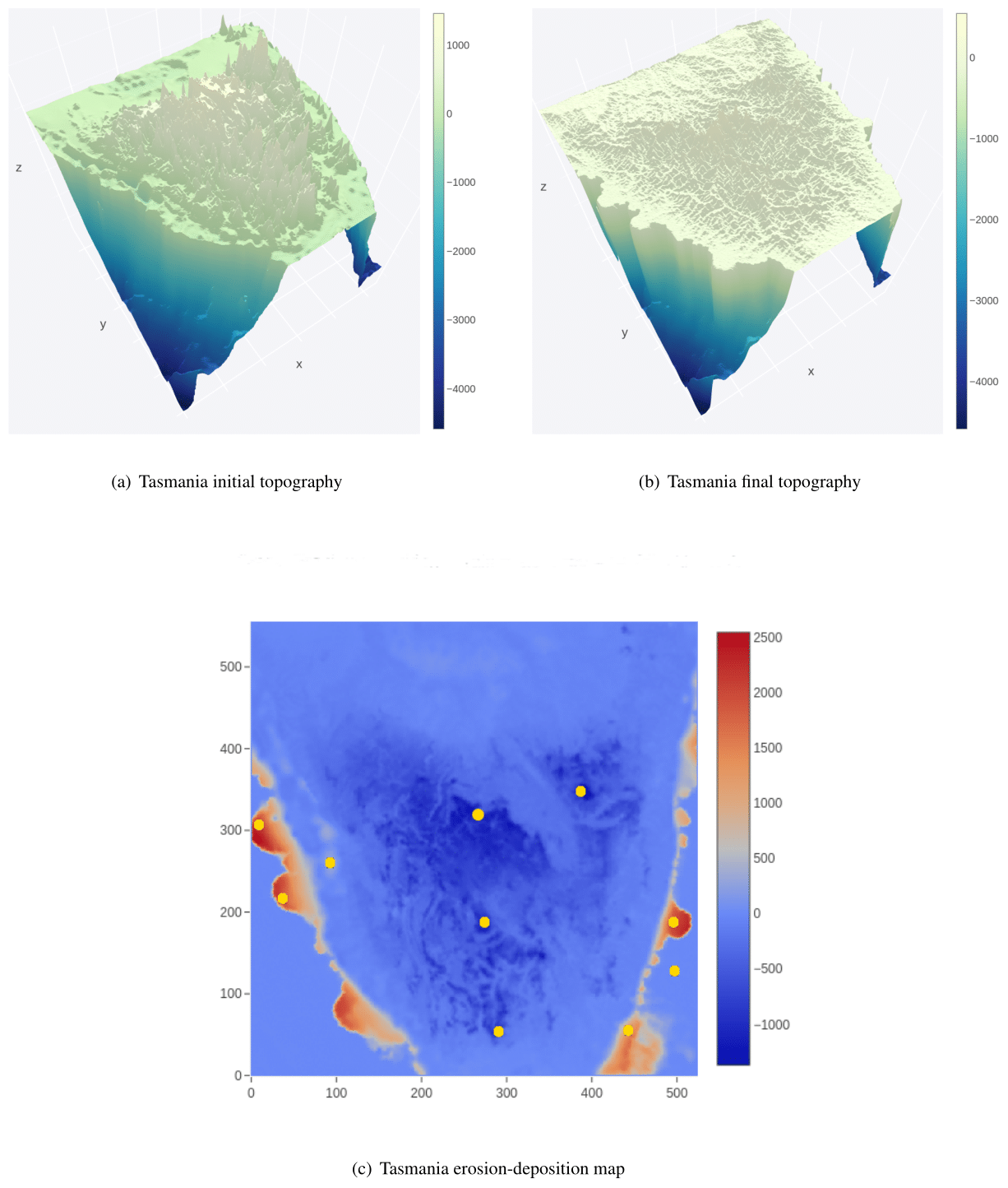
Figure 3Tasmania: initial and eroded ground-truth topography along with erosion–deposition that shows sediment deposition after 1 million years evolution. Note that x axis represents the latitude; y axis represents the longitude, and that aligns with Fig. 1b for the Tasmania problem. The elevation in metres (m) is given by the z axis, which is further shown as a colour bar.
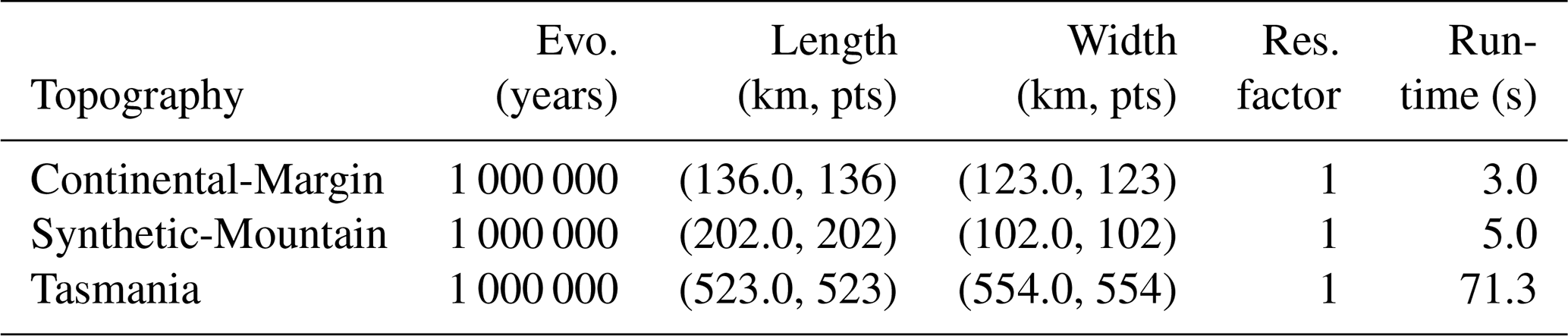
Table 1In the given landscape evolution problems, the run time represents approximately the duration for one model to run on a single CPU. The length and width are given in kilometres (km), which are represented by the specified number of points (pts) as defined by the resolution (Res.) factor.
2.2 Badlands model and Bayeslands framework
LEMs incorporate different driving forces such as tectonics or climate variability (Whipple and Tucker, 2002; Tucker and Hancock, 2010; Salles et al., 2018; Campforts et al., 2017; Adams et al., 2017) and combine empirical data and conceptual methods into a set of mathematical equations. Badlands (basin and landscape dynamics) (Salles et al., 2018; Salles and Hardiman, 2016) is an example of such a model that can be used to reconstruct landscape evolution and associated sediment fluxes (Howard et al., 1994; Hobley et al., 2011). Badlands LEM model (Salles et al., 2018) simulates landscape evolution and sediment transport/deposition with given parameters such as the precipitation rate and rock erodibility coefficient. The Badlands LEM simulates landscape dynamics, which requires an initial topography exposed to climate and geological factors over time.
Bayeslands essentially provides the estimation of unknown Badlands parameters with Bayesian inference via MCMC sampling (Chandra et al., 2019c). We use the final or present-day topography at time T and expected sediment deposits at selected intervals to evaluate the quality of proposals during sampling. In this way, we constrain the set of unknown parameters (θ) using ground-truth data (D). The prior distribution (also known as prior) refers to one's belief in the distribution of the parameter without taking into account the evidence or data. Bayeslands estimates θ so that the simulated topography by Badlands can resemble the ground-truth topography D to some degree. Bayeslands samples the posterior distribution p(θ|D) using principles of Bayes' rule
where, p(D|θ) is the likelihood of the data given the parameters, p(θ) is the prior, and p(D) is a normalizing constant and equal to . We note that the prior ratio cancels out since we use a uniform distribution for the priors.
3.1 Benchmark landscape evolution problems
We select two benchmark landscape problems from parallel tempering Bayeslands (Chandra et al., 2019c) that are adapted from earlier work (Chandra et al., 2019a). These include Continental-Margin (CM) and Synthetic-Mountain (SM), which are chosen due to the computational time taken for running a single model since they use less than 5 s to run a single model on a single central processing unit (CPU). These problems are well suited for a parameter evaluation for the proposed surrogate-assisted Bayesian inversion framework. In order to demonstrate an application which is computationally expensive, we introduce another problem, which features the landscape evolution of Tasmania in Australia for a million years that features the region shown in Fig. 1b. The Synthetic-Mountain landscape evolution is a synthetic problem, while the Continental-Margin problem is a real-world problem based on the topography of a region along the eastern margin of Te Waipounamu/South Island of Aotearoa/New Zealand as shown in Fig. 1a. We use Badlands to evolve the initial landscape with parameter settings given in Tables 1 and 2 and create the respective problems synthetic ground-truth topography.
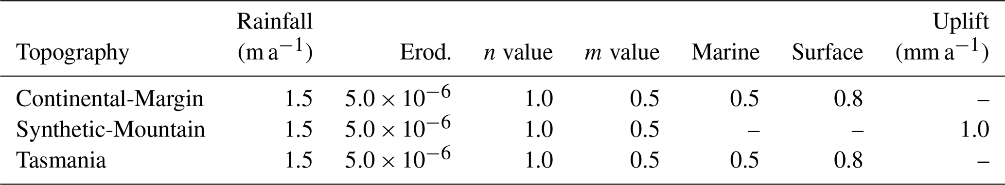
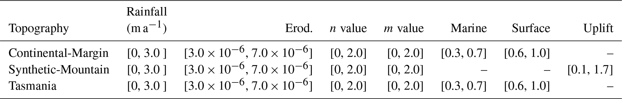
The initial and synthetic ground-truth topographies along with erosion/deposition for these problems appear in Figs. 2 and 3, respectively. Note that the figure shows that the Synthetic-Mountain is flat in the beginning, then given a constant uplift rate, along with weathering with constant precipitation rate, which creates the mountain topography. We use present-day topography as the initial topography in the Continental-Margin and Tasmania problems, whereas we use a synthetic flat region for Synthetic-Mountain initial topography. The problems involve an erosion–deposition model history that is used to generate synthetic ground-truth data for the final model state that we then attempt to recover. Hence, the likelihood function given in the following subsection takes both the landscape topography and erosion–deposition ground truth into account. The Continental-Margin and Tasmania cases feature six free parameters (Table 2), whereas the Synthetic-Mountain features five free parameters. Note that the marine diffusion coefficients are absent for the Synthetic-Mountain problem since the region does not cover or overlap with coastal and marine areas. The main reason behind choosing the two benchmark problems is due to their nature, i.e. the Synthetic-Mountain problem features uplift rate, which is not present in the Continental-Margin problem. The Continental-Margin problem features other parameters such as the marine coefficients. The Tasmania problem features a much bigger region; hence, it takes more computational time for running a single model. The common feature in all three problems is that they model both the elevation and erosion/deposition topography. Furthermore, we draw the priors from a uniform distribution with a lower and upper limit given in Table 3.
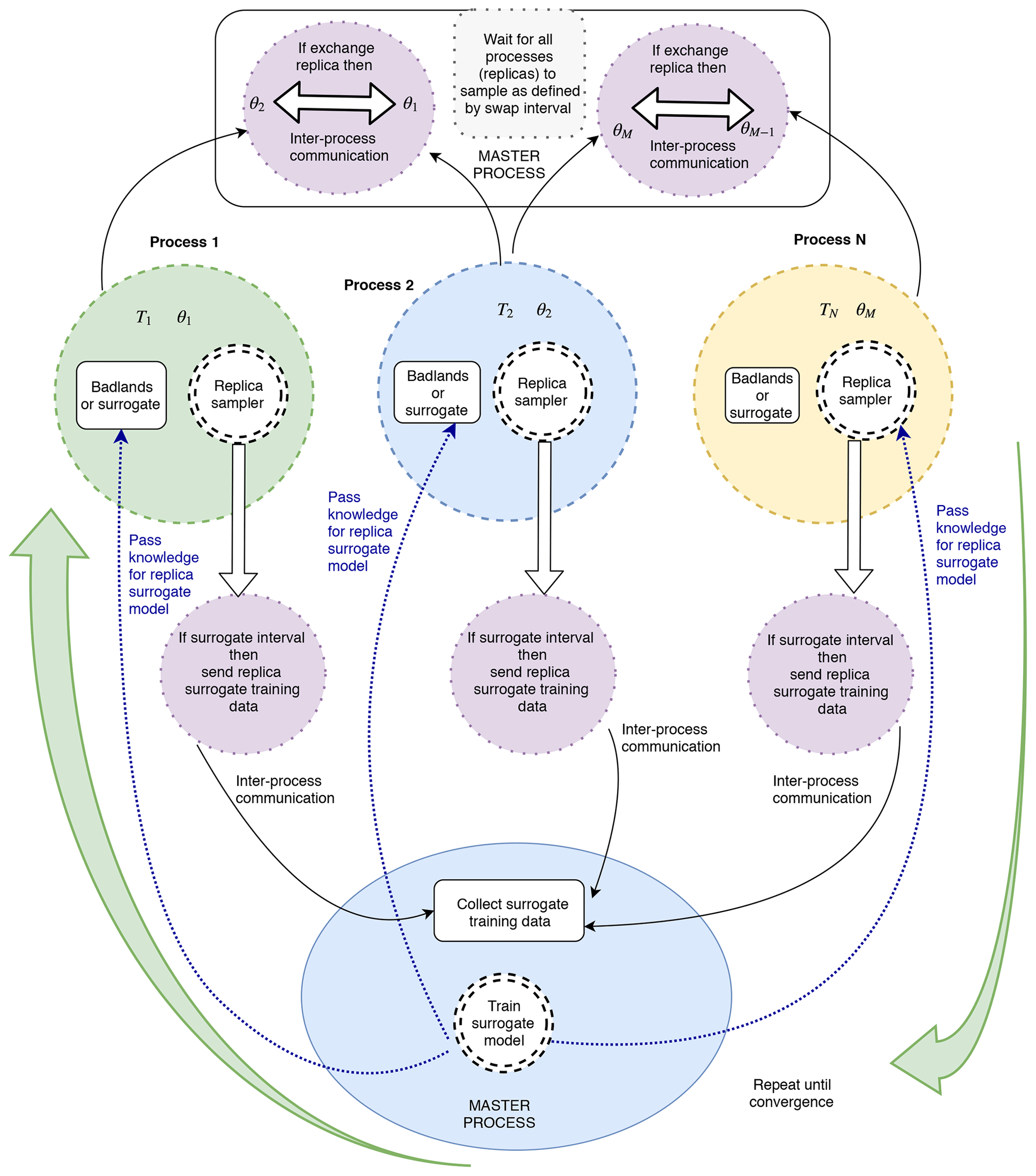
Figure 4Surrogate-assisted Bayeslands using the parallel tempering MCMC framework. We carry out the training in the master (manager) process, which features the global surrogate model. The replica processes provide the surrogate training dataset to the master process using inter-process communication. We employ a neural network model for the surrogate model. After training, we transfer the knowledge (neural network weights) to each of the replicas to enable estimation of pseudo-likelihood. Refer to Algorithm 1 for further details.
3.2 Bayeslands likelihood function
The Bayeslands likelihood function evaluates Badlands topography simulation along with the successive erosion–deposition, which denotes the sediment thickness evolution through time. More specifically, the likelihood function evaluates the effect of the proposals by taking into account the difference between the final simulated Badlands topography and the ground-truth topography. The likelihood function also considers the difference between the simulated and ground-truth sediment thickness at selected time intervals, which has been adapted from previous work (Chandra et al., 2019c) and is given as follows. The initial topography is denoted by D0 with , where si corresponds to site si, with the coordinates given by the latitude ui and longitude vi.
We assume an inverse gamma (IG) prior and integrate it so that the likelihood for the topography at time t=T is
where ν is the number of observations, and the subscript “l” in Ll(θ) denotes that it is the landscape likelihood to distinguish it from a sediment likelihood.
Although Badlands produces successive time-dependent topographies, only the final topography DT is used for the calculation of the elevation likelihood since little ground-truth information is available for the detailed evolution of surface topography. In contrast, the time-dependence of sedimentation can be used to ground-truth the time-dependent evolution of surface process models that include sediment transportation and deposition. The sediment erosion/deposition values at time (zt) are simulated (predicted) by the Badlands model given set of parameters, θ, plus some Gaussian noise as follows:
The sediment likelihood Ls(θ), after integrating out χ2, becomes
The combined likelihood takes both elevation and sediment/deposition into account
Note that although we used the log-likelihood version in our actual implementation, we refer to it as the likelihood throughout the paper.
3.3 Surrogate-assisted Bayeslands
The surrogate model learns from the relationship between the set of input parameters and the response given by the true (Badlands) model. The input is the set of proposals by the respective replica samplers in the parallel tempering MCMC sampling algorithm. We refer to the likelihood estimation by the surrogate model as the pseudo-likelihood.
We need to take into account the cost of inter-process communication in parallel computing environment to avoid computational overhead. As given in our previous implementation (Chandra et al., 2019c), the swap interval refers to the number of iterations after which each replica pauses and can undergo a replica transition. After the swap proposal is accepted or rejected, the respective replica sampling is resumed while undergoing Metropolis transition in between the swap intervals. We incorporate the surrogate-assisted estimation into the multicore parallel tempering algorithm. Our previous work (Chandra et al., 2020) used a surrogate interval that determines the frequency of training by collecting the history of past samples with their likelihood from the respective replicas. We need a swap interval of several samples when dealing with small-scale models that take a few seconds to run; however for large models, we recommend having a swap interval of 1.
Table 4Neural network architecture for the different problems.
Taking into account that the true model is represented as y=f(x), the surrogate model provides an approximation in the form ; such that , where e represents the difference or error. The task of the surrogate model is to provide an estimate for the pseudo-likelihood by training from the history of proposals, which is given by the set of input xr,s and likelihood ys, where “s” represents the sample and “r” represents the replica. Hence, we create the training dataset Φ for the surrogate by fusion of xr,s across all the replica for a given surrogate interval ψ, which can be formulated as follows:
where, xr,s represents the set of parameters proposed at sample “s”, is the likelihood, which is dependent on data and the Badlands model, and M is the total number of replicas. Θ denotes the training surrogate dataset, which features input Φ and response λ at the end of every surrogate interval denoted by s+ψ. Therefore, we give the pseudo likelihood as , where is the prediction from the surrogate model. The likelihood in training data is altered, with respect of the temperature, since it has been changed by taking Llocal∕Tr for given replica “r”. We undo this change by multiplying the likelihood by the respective replica temperature level taken from the geometric temperature ladder.
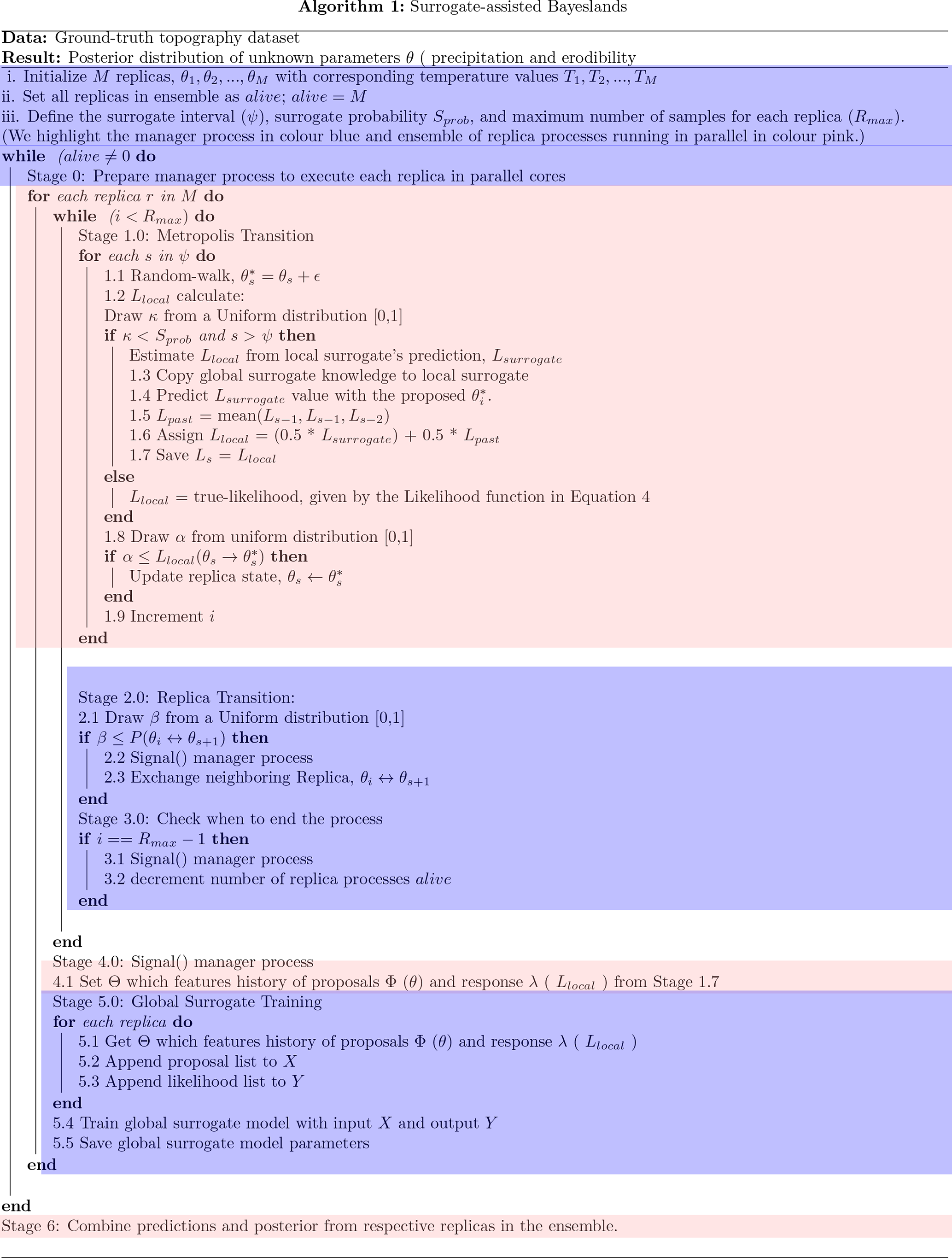
We present surrogate-assisted Bayeslands in Algorithm 1, which features parallel processing of the ensemble of replicas. The highlighted region in the colour pink of the Algorithm 1 shows different processing cores running in parallel, shown in Fig. 4 where the manager process is highlighted. Due to multiple parallel processing replicas, it is not straightforward to implement when to terminate sampling. Hence, the termination condition waits for all the replica processes to end as it monitors the number of active or alive replica processes in the manager process. We begin by setting the number of alive replicas in the ensemble (alive = M) and then the replicas that sample θn are assigned values using a uniform distribution ; where α defines the range of the respective parameters. We then assign the user-defined parameters, which include the number of replica samples Rmax, swap-interval Rswap, surrogate interval, ψ, and surrogate probability Sprob, which determines the frequency of employing the surrogate model for estimating the pseudo-likelihood.
Table 6Convergence diagnosis (PSRF score) for Continental-Margin problem.
The samples that cover the first surrogate interval makes up the initial surrogate training data Θ, which feature all the replicas. We then train the surrogate to estimate the pseudo-likelihood when required according to the surrogate probability. Figure 4 shows how the manager processing unit controls the respective replicas, which samples for the given surrogate interval. Then, the algorithm calculates the replica transition probability for the possibility of swapping the neighbouring replicas. The information flows from replica process to manager process using signal() via inter-process communication given by the replica process as shown in Stage 2.2, 3.1, and 4.0 of Algorithm 1, and further shown in Fig. 4.
To enable better estimation for the pseudo-likelihood, we retrain the surrogate model for remaining surrogate interval blocks until the maximum time (Rmax). We train the surrogate model only in the manager process and the algorithm passes the surrogate model copy with the trained parameters to the ensemble of replica processes for predicting or estimating the pseudo-likelihood. The samples associated with the true-likelihood only becomes part of the surrogate training dataset. In Stage 1.4 of Algorithm 1, the pseudo-likelihood (Lsurrogate) provides an estimation with given proposal . Stage 1.5 calculates the likelihood moving average of past three likelihood values, Lpast = mean(). In Stage 1.6, we combine the moving average likelihood with the pseudo-likelihood to give a prediction that considers the present replica proposal and taking into account the past, Llocal = (0.5×Lsurrogate) + 0.5×Lpast. The surrogate training can consume a significant portion of time, which is dependent on the size of the problem in terms of the number of parameters and also the type of surrogate model used, along with the training algorithm. We evaluate the trade-off between quality of estimation by pseudo-likelihood and overall cost of computation for the true likelihood function for different types of problems.
We validate the quality of estimation from the surrogate model by the root-mean-squared error (RMSE), which considers the difference between the true likelihood and the pseudo-likelihood. This can be seen as a regression problem with multi-input (parameters) and a single output (likelihood). Hence, we report the surrogate prediction quality by
where yi and are the true likelihood and the pseudo-likelihood values, respectively. N is the number of cases the surrogate has used during sampling.
We further note that the framework uses parallel tempering MCMC in the first stage of sampling and then transforms into the second stage where the temperature ladder is changed such that Ti=1, for all replicas, i=1, 2, ..., M. This strategy enables exploration in the first stage and exploitation in the second stage. We combine the respective replica posterior distributions once the termination condition is met and show their mean and standard deviation of the prediction in the results.
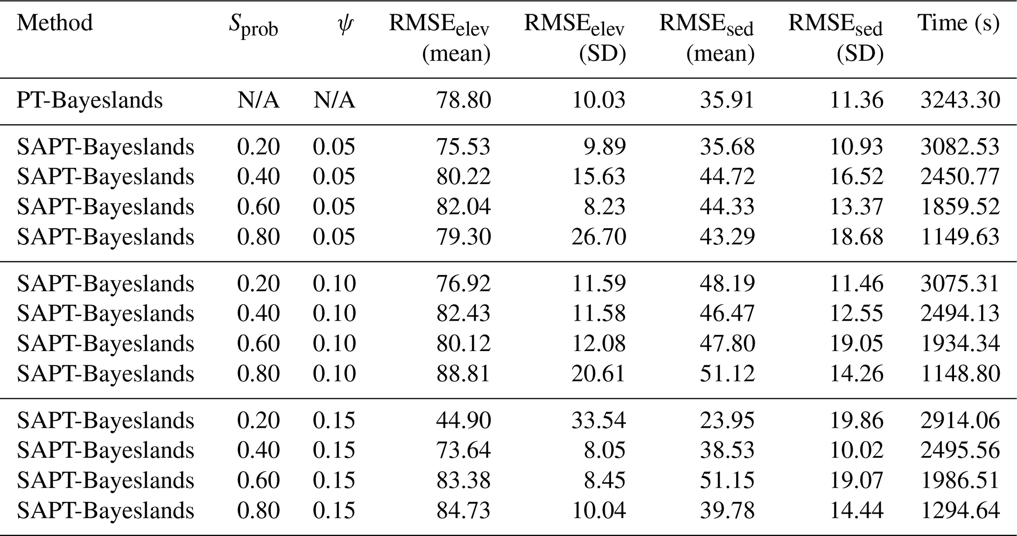
Table 8Performance comparison for respective problems and methods. N/A: not applicable.

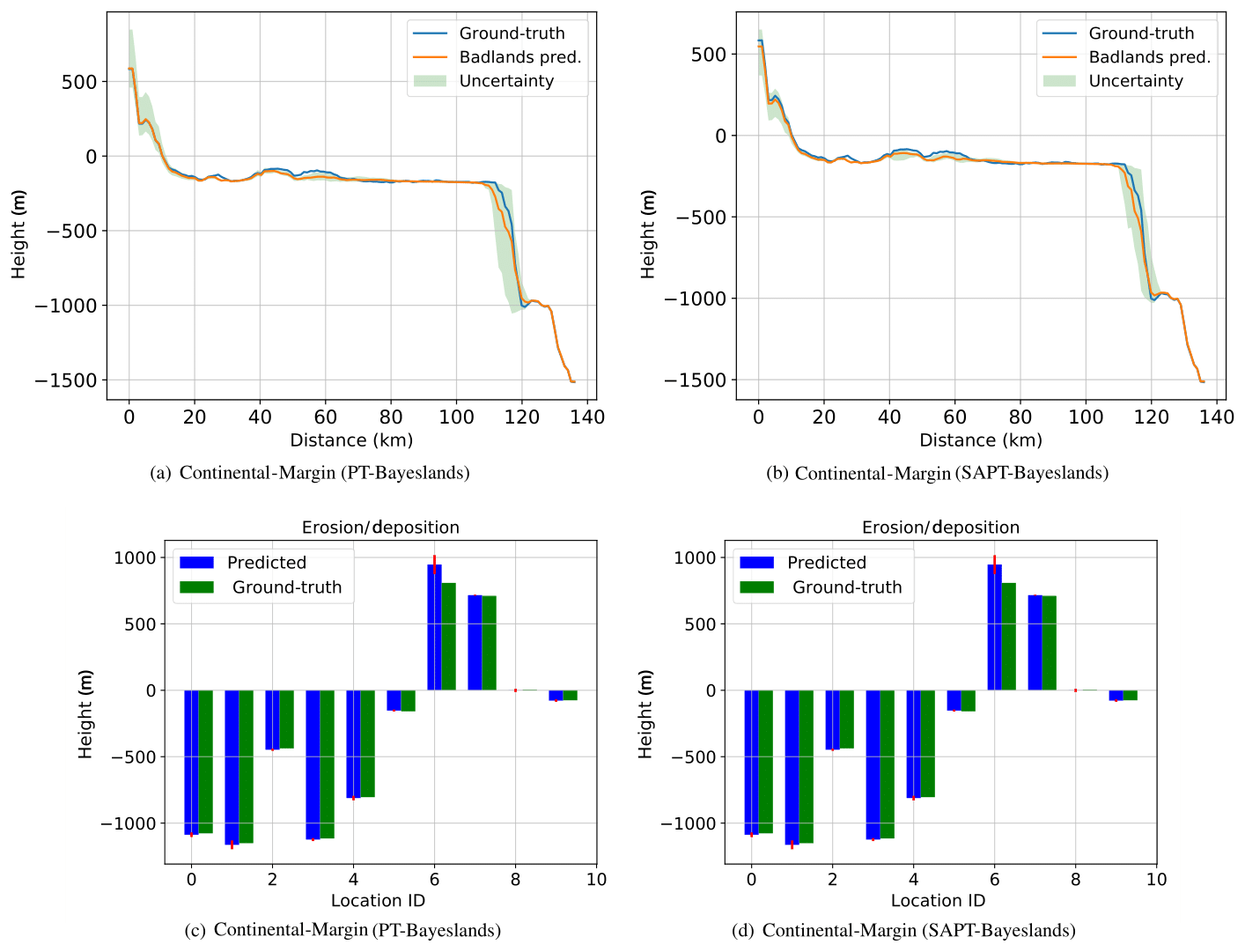
Figure 5Topography cross section and erosion–deposition prediction for 10 chosen points (selected coordinates denoted by location identifier, ID, number) for Continental-Margin problem from results summarized in Table 8.
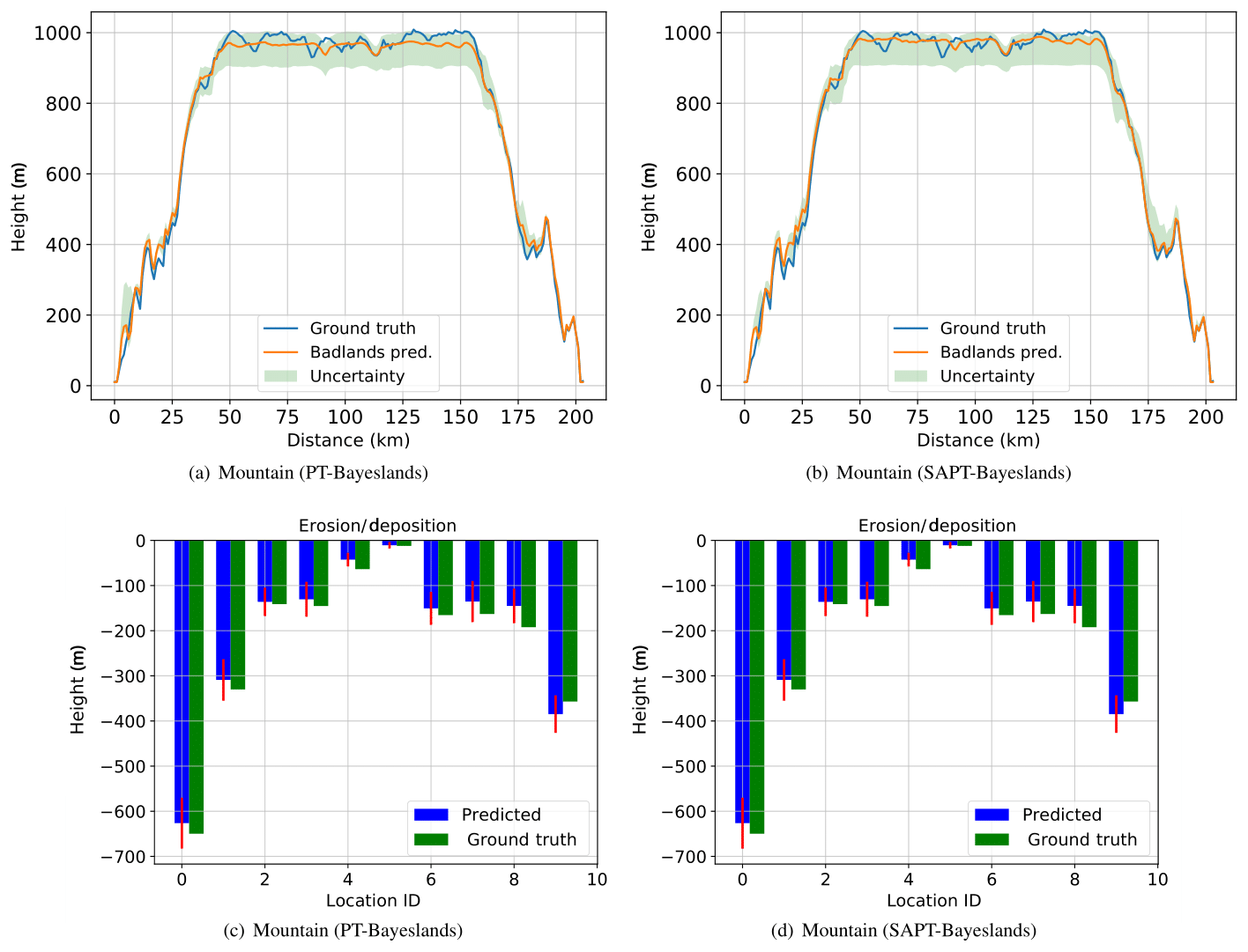
Figure 6Topography cross section and erosion–deposition prediction for 10 chosen points (selected coordinates denoted by location identifier (ID) number) for Synthetic-Mountain problem from results summarized in Table 8.
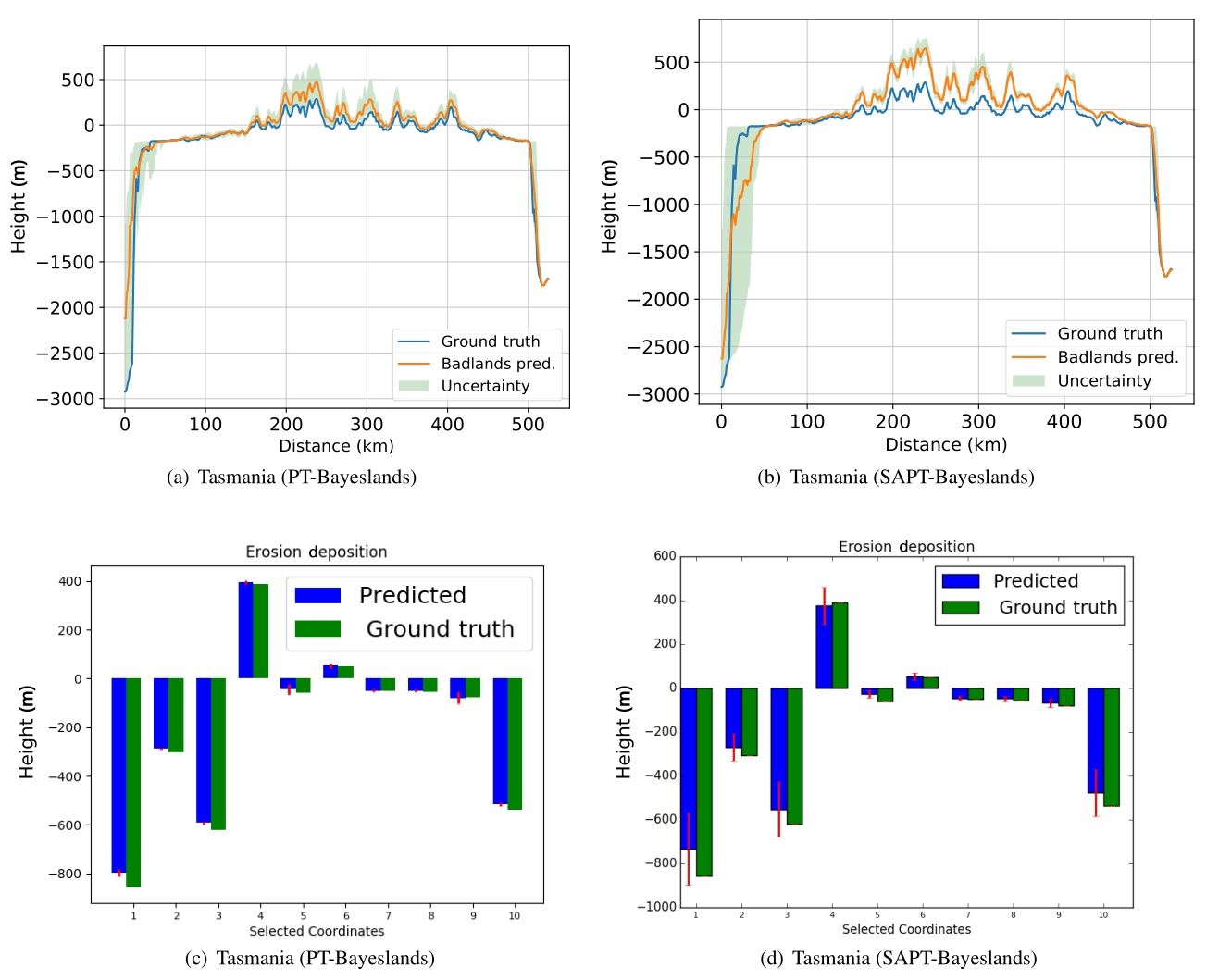
Figure 7Topography cross section and erosion–deposition prediction for 10 chosen points (selected coordinates denoted by location identifier, ID, number) for Tasmania problem from results summarized in Table 8.
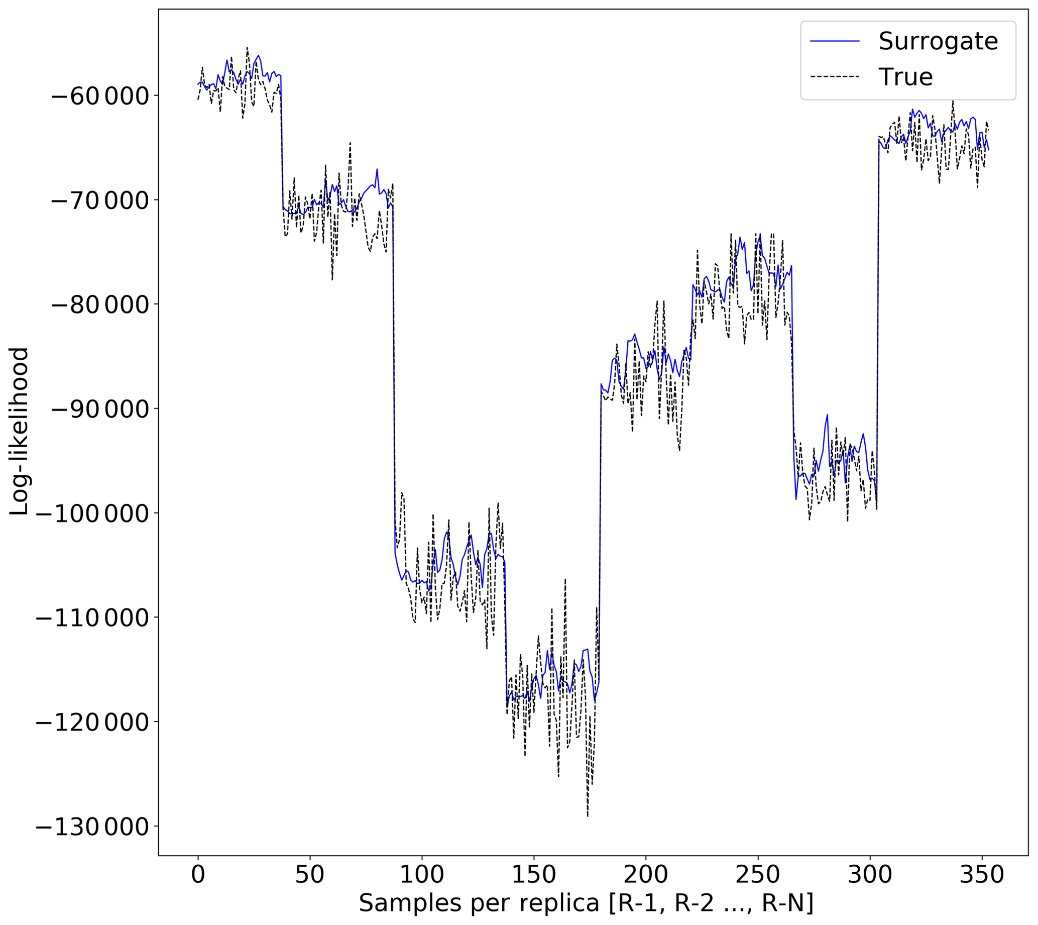
Figure 8Surrogate likelihood vs. true likelihood estimation for Continental-Margin problem (RMSEsur=3605).
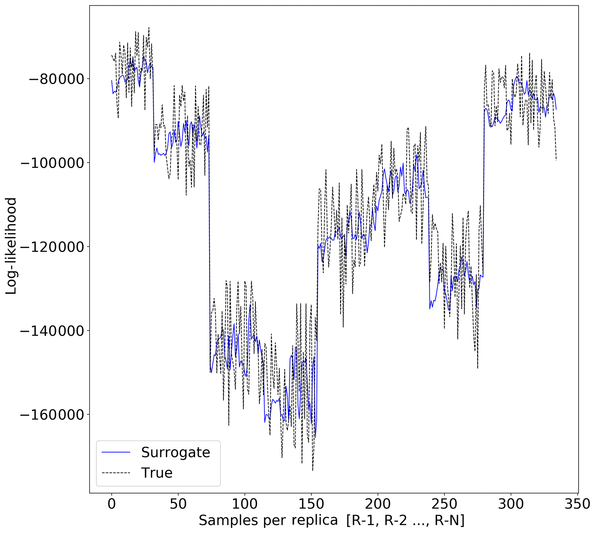
Figure 9Surrogate likelihood vs. true likelihood estimation for Synthetic-Mountain problem (RMSEsur=9917).
We evaluate the prediction performance by comparing the predicted/simulated Badlands landscape with the ground-truth data using the root-mean-squared error (RMSE). We compute the RMSE for the elevation (elev) and sediment erosion/deposition (sed) at each iteration of the sampling scheme using
where is an estimated value of θ, and θ is the true value representing the synthetic ground truth. f(.) and g(.) represent the outputs of the Badlands model, while m and n represent the size of the selected topography. v is the number of selected points from sediment erosion/deposition over the selected time frame, nt.
3.4 Surrogate model
To choose a particular surrogate model, we need to consider the computational resources for training the model during the sampling process. The literature review showed that Gaussian process models, neural networks, and radial basis functions (Broomhead and Lowe, 1988) are popular choices for surrogate models. We note that Badlands LEM features about a dozen free parameters in one of the simplest cases; this increases when taking into account spatial and temporal dependencies. For instance, the precipitation rate for a million years can be represented by a single parameter or by 10 different parameters that capture every 100 000 years for 10 different regions, which can account for 1000 parameters instead of 1. Considering hundreds or thousands of unknown Badlands model parameters, the surrogate model needs to be efficiently trained without taking lots of computational resources. The flexibility of the model to have incremental training is also needed, and hence, we rule out Gaussian process models since they have limitations in training when the size of the dataset increases to a certain level (Rasmussen, 2004). Therefore, we use neural networks as the choice of the surrogate model, and the training data and neural network model is formulated as follows.
We denote the surrogate model training data by Φ and λ, which is shown in Eq. (5), where Φ is the input, and λ is the desired output of the model. The prediction of the model is denoted by . We use a feedforward neural network as the surrogate model. Given input xt, f(xt) is computed by the feedforward neural network with one hidden layer defined by the function
where δo and δh are the bias weights for the output o and hidden h layer, respectively. vj is the weight which maps the hidden layer h to the output layer. wdh is the weight which maps xt to the hidden layer h, and g(.) is the activation function for the hidden and output layer units. We use ReLU (rectified linear unitary function) as the activation function. The learning or optimization task then is to iteratively update the weights and biases to minimize the cross-entropy loss J(W,b). This can be done using gradient update of weights using the Adam (adaptive moment estimation) learning algorithm (Kingma and Ba, 2014) and stochastic gradient descent (Bottou, 1991, 2010). We experimentally evaluate them for training the feedforward network for the surrogate model in the next section.
3.5 Proposal distribution
Bayeslands features random-walk (RW) and adaptive-random-walk (ARW) proposal distributions which will be evaluated further for surrogate-assisted Bayeslands in our experiments. In our previous work (Chandra et al., 2019a), ARW showed better convergence properties when compared to RW proposal distribution. The RW proposal distribution features Σ as the diagonal matrix, so that , where σj is the step size of the jth element of the parameter vector θ. The step size for θj is a combination of a fixed step size ϕ, which is common to all parameters, multiplied by the range of possible values for parameter θj; hence , where aj and bj represent the maximum and minimum limits of the prior for θj given in Table 2. In our experiments, the RW proposal distribution employs fixed step size, ϕ=0.05,
The ARW proposal distribution features adaptation of the diagonal matrix Σ at every K interval of within-replica sampling. It allows for the dependency between elements of θ and adapts during sampling (Haario et al., 2001). We adapt the elements of Σ for the posterior distribution using the sample covariance of the current chain history , where θ[i] is the ith iterate of θ in the chain, and λj is the minimum allowed step sizes for each parameter θj.
3.6 Design of experiments
We demonstrate effectiveness of surrogate-assisted parallel tempering (SAPT-Bayeslands) framework for selected Badlands LEMs taken from our previous study (Chandra et al., 2019c).
We first investigate the effects of different surrogate training procedures and parameter evaluation for SAPT-Bayeslands using smaller synthetic problems. Afterwards, we apply the methodology to a larger landscape evolution problem, which is Tasmania, Australia. We design the experiments as follows.
-
We generate a dataset for training and testing the surrogate for the Synthetic-Mountain and Continental-Margin landscape evolution problems. We use the neural network model for the surrogate and evaluate different training techniques.
-
We evaluate if the transfer of knowledge from previous surrogate interval is better than no transfer of knowledge for Synthetic-Mountain and Continental-Margin problems. Note this is done only with the data generated from the previous step.
-
We provide convergence diagnosis for the RW and ARW proposal distributions in PT-Bayeslands and SAPT-Bayeslands.
-
We integrate the surrogate model into Bayeslands and evaluate the effectiveness of the surrogate in terms of estimation of the likelihood and computational time. Due to the computational requirements, we only consider the Continental-Margin problem.
-
We then apply SAPT-Bayeslands to all the given problems and compare with PT-Bayeslands.
We use Keras neural networks library (Gulli and Pal, 2017) for implementation of the surrogate. We provide the open-source software package that implements Algorithm 1 along with benchmark problems and experimental results 1.
We use a geometric temperature ladder with a maximum temperature of Tmax=2 for determining the temperature level for each of the replicas. In trial experiments, the selection of these parameters depended on the performance in terms of the number of accepted samples and prediction accuracy of elevation and sediment/deposition. We use replica-exchange or swap interval value; Rswap=3 samples that determine when to check whether to swap with the neighbouring replica. In previous work (Chandra et al., 2019c), we observed that increasing the number of replicas up to a certain point does not necessarily mean that we get better performance in terms of the computational time or prediction accuracy. In this work, we limit the number of replicas to Rnum=8 for all experiments with maximum of 5000 samples.
We use a 50 % burn in, which discards the portion of samples in the parallel tempering MCMC stage as done in our previous work (Chandra et al., 2019a).
4.1 Surrogate accuracy
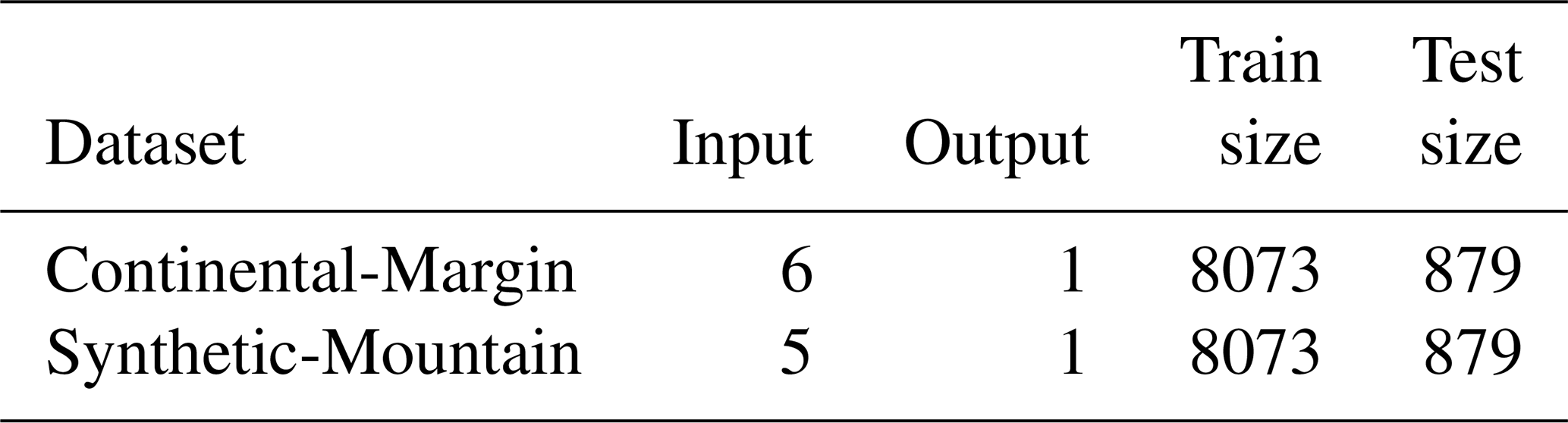
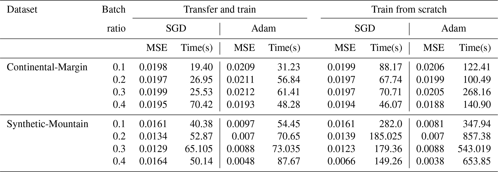
To implement the surrogate model, we need to evaluate the training algorithm, such as Adam and stochastic gradient descent (SGD). Furthermore, we also evaluate specific parameters, such as the size of the surrogate interval (batch ratio), the neural network topology for the surrogate, and the effectiveness of either training from scratch or utilizing previous knowledge for surrogate training (transfer and train). We create a training dataset from the cases where the true likelihood was used, which compromises the history of the set of parameters proposed with the corresponding likelihood. This is done for standalone evaluation of the surrogate model, which further ensures that the experiments are reproducible since different experimental runs create different datasets depending on the exploration during sampling. We then evaluate the neural network model designated for the surrogate using two major training algorithms which featured the Adam optimizer and stochastic gradient descent. The parameters that define the neural network surrogate model used for the experiments are given in Table 4. Note that the train size in Table 4 refers to the maximum size of the dataset. The training is done in batches where the batch ratio determines the training dataset size, as shown in Table 5.
Table 5 presents the results for the experiments that took account of the training data collected during sampling for two benchmark problems (Continental-Margin and Synthetic-Mountain). Note that we report the mean value of the mean-squared-error (MSE) for the given batch ratio from 10 experiments. The batch ratio is taken, in relation to the maximum number of samples across the chains (Rmax∕Rnum). We normalize the likelihood values (outcomes) in the dataset to the range [0,1]. In most cases, the accuracy of the neural network is slightly better when training from scratch with combined data; however, there is a considerable trade-off with the time required to train the network. The results show that the transfer and train methodology, in general, requires much lower computational time when compared to training from scratch with combined data. Moreover, in comparison to SGD and Adam training algorithms, we observe that SGD achieves slightly better accuracy than Adam for Continental-Margin problem. However, Adam, having an adaptive learning rate, outperforms SGD in terms of the time required to train the network. Thus, we can summarize that transfer and train method is better since it saves significant computation time with a minor trade-off with accuracy.
4.2 Convergence diagnosis
The Gelman–Rubin diagnostic (Gelman and Rubin, 1992) is one of the popular methods used for evaluating convergence by analysing the behaviour of multiple Markov chains. The assessment is done by comparing the estimated between-chain and within-chain variances for each parameter, where large differences between the variances indicate non-convergence. The diagnosis reports the potential scale reduction factor (PSRF), which gives the ratio of the current variance in the posterior variance for each parameter compared to that being sampled, and the values for the PSRF near 1 indicates convergence. We analyse five experiments for each case using different initial values for 5000 samples for each problem configuration.
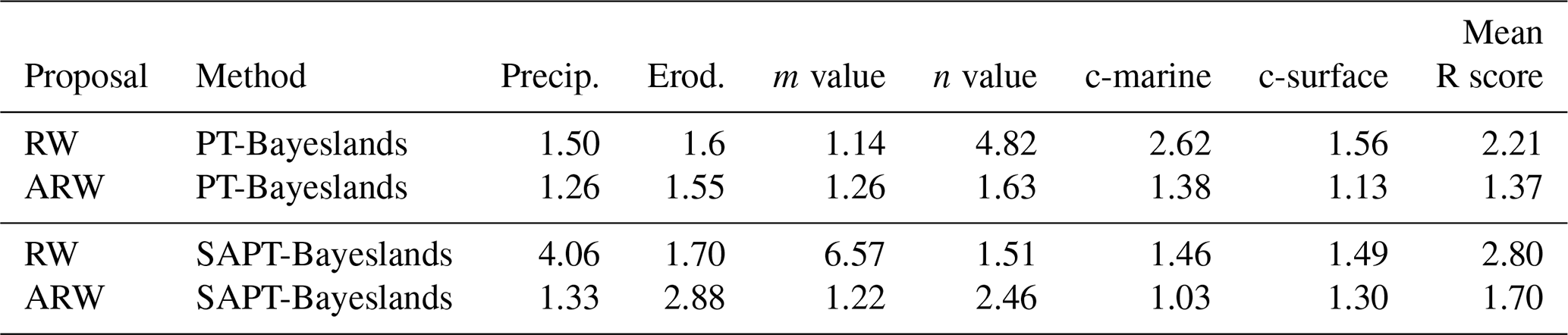
Table 6 presents the convergence diagnosis using the PSRF score for RW and ARW proposal distributions for PT-Bayeslands and SAPT-Bayeslands. We notice that ARW has a lower PSRF score (mean) when compared to the RW proposal distribution, which indicates better convergence. We also notice that the ARW SAPT-Bayeslands maintains convergence with a PSRF score close to ARW PT-Bayeslands when compared to rest of the configurations. This suggests that although we use surrogates, convergence can be maintained up to a certain level, which is better than RW PT-Bayeslands.
4.3 Surrogate-assisted Bayeslands
We investigate the effect of the surrogate probability (Sprob) and surrogate interval (ψ) on the prediction accuracy (RMSEelev and RMSEsed) and computational time. Note that we report the prediction accuracy mean and standard deviation (mean and SD) of accepted samples over the sampling time after removing the burn-out period. We report the computational time in seconds (s). Table 7 presents the performance of the respective methods (PT-Bayeslands and SAPT-Bayeslands) with respective parameter settings for the Continental-Margin problem. In SAPT-Bayeslands, we observe that there is not a major difference in the accuracy of elevation or erosion/deposition given different values of Sprob. Nevertheless, there is a significant difference in terms of the computational time where higher values of Sprob save computational time. Furthermore, we notice that there is not a significant difference in the prediction accuracy given different values of ψ, which suggests that the selected values are sufficient.
We select a suitable combination of the set of parameters evaluated in the previous experiment (Sprob=0.6 and ψ=0.05) and apply them to rest of the problems. Table 8 gives a comparison of performance for Continental-Margin and Synthetic-Mountain problems, along with the Tasmania one, which is a bigger and more computationally expensive problem. We notice that the performance of SAPT-Bayeslands is similar to PT-Bayeslands, while a significant portion of computational time is saved.
Figures 5, 6, and 7 provide a visualization of the elevation prediction accuracy when compared to actual ground truth between the given methods from results given in Table 8. We also provide the prediction accuracy of erosion/deposition for 10 chosen points taken at selected locations. Although both methods provide erosion/deposition prediction for four successive time intervals, we only show the final time interval. In both the Continental-Margin and Synthetic-Mountain problems, we notice that the prediction accuracy of PT-Bayeslands is very similar to SAPT-Bayeslands, and the Badlands prediction of the topography is close to ground truth, within the credible interval. This indicates that the use of surrogates has been beneficial where no major loss in accuracy in prediction is given. In the case of the Tasmania problem, there is a loss in Badlands prediction accuracy, which could be due to the size of the problem. Nevertheless, this loss is not that clear from results in Table 8. It could be that the topography prediction is mostly inconsistent at the cross section where it features mountainous regions.
Figures 8 and 9 show the true likelihood and prediction by the surrogate for the Continental-Margin and Synthetic-Mountain problems, respectively. We notice that at certain intervals given in Fig. 8, given by different replica, there is inconsistency in the predictions. Moreover, Fig. 9 shows that the log-likelihood is very chaotic, and hence there is difficulty in providing robust prediction at certain points in the time given by samples for the respective replica.
4.4 Discussion
We observe that the surrogate probability is directly related to the computational performance; this is obvious since computational time depends on how often we use the surrogate. Our concern is the prediction performance, especially while increasing the use of the surrogate as it could lower the accuracy, which can result in a poor estimation of the parameters. According to the results, the accuracy is well retained given a higher probability of using surrogates. In the cross section presented in the results for Continental-Margin and Synthetic-Mountain problems, we find that there is not much difference in the accuracy given in prediction by the SAPT-Bayeslands when compared to PT-Bayeslands. Moreover, in the application to a more computationally intensive problem (Tasmania), we find that a significant reduction in computational time is achieved. Although we demonstrated the method using small-scale models that run within a few seconds to minutes, the computational costs of continental-scale Badlands models are extensive. For instance, the computational time for a 5 km resolution for the Australian continent Badlands model for 149 million years is about 72 h; hence, in the case when thousands of samples are required, the use of surrogates can be beneficial. We note that improved efficiency of the surrogate-assisted Bayeslands comes at the cost of accuracy for some problems (in case of the Tasmania problem), and there is a trade-off between accuracy and computational time.
In future work, rather than a global surrogate model, we could use the local surrogate model on its own, where the training only takes place in the local surrogates by relying on the history of the likelihood and hence taking a univariate time series prediction approach using neural networks. Our primary contribution is in terms of the parallel-computing-based open-source software and the proposed underlying framework for incorporating surrogates, taking into account complex issues such as inter-process communication. This opens the road to using different types of surrogate models while using the underlying framework and open-source software. Given that the sediment erosion/deposition is temporal, other ways of formulating the likelihood could be possible; for instance, we could have a hierarchical Bayesian model with two stages for MCMC sampling (Chib and Carlin, 1999; Wikle et al., 1998).
The initial evaluation for the setup surrogate model shows that it is best to use a transfer learning approach where the knowledge from the past surrogate interval is utilized and refined with new surrogate data. This consumes much less time than accumulating data and training the surrogate from scratch at every surrogate interval. We note that in the case when we use the surrogate model for pseudo-likelihood, there is no prediction given by the surrogate model. The prediction (elevation topography and erosion–deposition) during sampling are gathered only from the true Badlands model evaluation rather than the surrogate. In this way, one could argue that the surrogate model is not mimicking the true model; however, we are guiding the sampling algorithm towards forming better proposals without evaluation of the true model. A direction forward is in incorporating other forms of surrogates, such as running a low-resolution Badlands model as the surrogate, which would be computationally faster in evaluating the proposals; however, limitations in terms of the effect of resolution setting on Badlands topography simulation may exist.
Furthermore, computationally efficient implementations of landscape evolution models that only feature landscape evolution (Braun and Willett, 2013) could be used as the surrogate, while we could use Badlands model that features both landscape evolution and erosion/deposition as the true model. We could also use computationally efficient implementations of landscape evolution models that consider parallel processing (Hassan et al., 2018) in the Bayeslands framework. In this case, the challenge would be in allocating specialized processing cores for Badlands and others for parallel tempering MCMC.
We adapted the surrogate framework developed for machine learning (Chandra et al., 2020) with a different proposal distribution instead of using gradient-based proposals. Gradient-based parameter estimation has been very popular in machine learning due to availability of gradient information. Due to the complexity in geological or geophysical numerical forward models, it is challenging to obtain gradients, which has been the case for the Badlands landscape evolution model. We used random-walk and adaptive-random-walk proposal distributions which have limitations; hence, we need to incorporate advanced meta-heuristic techniques to form non-gradient-based proposals for efficient search. Our study is limited to a relatively small set of free parameters, and a significant challenge would be to develop surrogate models with an increased set of parameters.
We presented a novel application of surrogate-assisted parallel tempering that features parallel computing for landscape evolution models using Badlands. Initially, we experimented with two different approaches for training the surrogate model, where we found that a transfer learning-based approach is beneficial and could help reduce the computational time of the surrogate. Using this approach, we presented the experiments that featured evaluating certain key parameters of the surrogate-based framework. In general, we observed that the proposed framework lowers the computational time significantly while maintaining the required quality in parameter estimation and uncertainty quantification.
In future work, we envision applying the proposed framework to more complex applications such as the evolution of continental-scale landscapes and basins over millions of years. We could use the approach for other forward models such as those that feature geological reef development or lithospheric deformation. Furthermore, the posterior distribution of our parameters requires multimodal sampling methods; hence, a combination of meta-heuristics for proposals with surrogate-assisted parallel tempering could improve exploration features and also help in lowering the computational costs.
Parallel tempering MCMC features massive parallelism with enhanced exploration capabilities. It features several replicas with slight variations in the acceptance criteria through relaxation of the likelihood with a temperature ladder that affects the replica sampling acceptance criterion. The replicas associated with higher temperature levels have more chance in accepting weaker proposals, which could help in escaping a local minimum. Given an ensemble of M replicas defined by a temperature ladder, we define the state by , where xi is the replica at temperature level Ti. We construct a Markov chain to sample proposal xi and evaluate it using the likelihood L(xi) for each replica defined by temperature level Ti. At each iteration, the Markov chain can feature two types of transitions that include the Metropolis transition and the replica transition.
In the Metropolis transition phase, we independently sample each replica to perform local Monte Carlo moves as defined by the temperature ladder for the replica by relaxing or changing the likelihood in relation to the temperature level L(xi)∕Ti. We sample configuration from a proposal distribution . The Metropolis–Hastings ratio at temperature level Ti is given by
where L represents the likelihood at the local replica. We accept the new state with probability, min. The detailed balance condition holds for each MCMC replica; therefore, it holds for the ensemble system (Calderhead, 2014).
In the replica transition phase, we consider the exchange of the current state between two neighbouring replicas based on the Metropolis–Hastings acceptance criteria. Hence, given a probability α, we exchange a pair of replica defined by two neighbouring temperature levels, Ti and Ti+1.
The exchange of neighbouring replicas provides an efficient balance between local and global exploration (Sambridge, 2013). The temperature ladder and replica exchange have been of the focus of investigation in the past (Calvo, 2005; Liu et al., 2005; Bittner et al., 2008; Patriksson and van der Spoel, 2008), and there is a consensus that they need to be tailored for different types of problems given by their likelihood landscape. In this paper, the selection of temperature spacing between the replicas is carried out using a geometric spacing methodology (Vousden et al., 2015), given as follows:
where and Tmax is maximum temperature, which is user defined and dependent on the problem.
A1 Training the neural network surrogate model
We note that stochastic gradient descent maintains a single learning rate for all weight updates, and typically the learning rate does not change during the training. Adam (adaptive moment estimation) learning algorithm (Kingma and Ba, 2014) differs from classical stochastic gradient descent, as the learning rate is maintained for each network weight and separately adapted as learning unfolds. Adam computes individual adaptive learning rates for different parameters from estimates of first and second moments of the gradients. Adam features the strengths of root mean square propagation (RMSprop) and adaptive gradient algorithm (AdaGrad) (Kingma and Ba, 2014; Duchi et al., 2011). Adam has shown better results when compared to stochastic gradient descent, RMSprop, and AdaGrad. Hence, we consider Adam as the designated algorithm for the neural-network-based surrogate model. We formulate the learning procedure through weight update for iteration number t for weights W and biases b by
where mt and vt are the, respectively, first and second moment vectors for iteration t; β1 and β2 are constants ; α is the learning rate, and ϵ is a close to zero constant.
We provide open-source code along with data and sample results to motivate further work in this area: https://github.com/intelligentEarth/surrogateBayeslands (last access: 6 July 2020, intelligentEarth, 2020); https://doi.org/10.5281/zenodo.3892277 (Chandra, 2020).
RC led the project and contributed to writing the paper and designing the experiments. DA contributed by running experiments and providing documentation of the results. AK contributed in terms of programming, running experiments, and providing documentation of the results. RDM contributed by managing the project, writing the paper, and providing analysis of the results.
The authors declare that they have no conflict of interest.
We would like to thank Konark Jain for technical support. R. Dietmar Müller and Danial Azam were supported by the Australian Research Council (grant IH130200012). We sincerely thank the reviewers for their comments that helped us in improving the paper.
This research has been supported by the University of Sydney (grant no. SREI Grant 2017-2018) and the Australian Research Council (grant no. IH130200012).
This paper was edited by Richard Neale and reviewed by two anonymous referees.
Adams, J. M., Gasparini, N. M., Hobley, D. E. J., Tucker, G. E., Hutton, E. W. H., Nudurupati, S. S., and Istanbulluoglu, E.: The Landlab v1.0 OverlandFlow component: a Python tool for computing shallow-water flow across watersheds, Geosci. Model Dev., 10, 1645–1663, https://doi.org/10.5194/gmd-10-1645-2017, 2017. a
Ampomah, W., Balch, R., Will, R., Cather, M., Gunda, D., and Dai, Z.: Co-optimization of CO2 EOR and Storage Processes under Geological Uncertainty, Energy Proc., 114, 6928–6941, 2017. a
Asher, M. J., Croke, B. F., Jakeman, A. J., and Peeters, L. J.: A review of surrogate models and their application to groundwater modeling, Water Resour. Res., 51, 5957–5973, 2015. a
Bittner, E., Nußbaumer, A., and Janke, W.: Make life simple: Unleash the full power of the parallel tempering algorithm, Phys. Rev. Lett., 101, 130603, https://doi.org/10.1103/PhysRevLett.101.130603, 2008. a
Bottou, L.: Stochastic gradient learning in neural networks, Proc. Neuro-Nımes, 91, 12, 1991. a
Bottou, L.: Large-scale machine learning with stochastic gradient descent, in: Proceedings of COMPSTAT'2010, 177–186, Springer, 2010. a
Braun, J. and Willett, S. D.: A very efficient O(n), implicit and parallel method to solve the stream power equation governing fluvial incision and landscape evolution, Geomorphology, 180–181, 170–179, 2013. a
Broomhead, D. S. and Lowe, D.: Radial basis functions, multi-variable functional interpolation and adaptive networks, Tech. rep., Royal Signals and Radar Establishment Malvern (United Kingdom), 1988. a
Calderhead, B.: A general construction for parallelizing Metropolis-Hastings algorithms, P. Natl. Acad. Sci. USA, 111, 17408–17413, 2014. a
Calvo, F.: All-exchanges parallel tempering, The J. Chem. Phys., 123, 124106, https://doi.org/10.1063/1.2036969, 2005. a
Campforts, B., Schwanghart, W., and Govers, G.: Accurate simulation of transient landscape evolution by eliminating numerical diffusion: the TTLEM 1.0 model, Earth Surf. Dynam., 5, 47–66, https://doi.org/10.5194/esurf-5-47-2017, 2017. a
Chandra, R.: Surrogate-assisted Bayesian inversion for landscape and basin evolution models (Version 1.0), Geoscientific Model Development, Zenodo, https://doi.org/10.5281/zenodo.3892277, 2020. a
Chandra, R., Azam, D., Müller, R. D., Salles, T., and Cripps, S.: BayesLands: A Bayesian inference approach for parameter uncertainty quantification in Badlands, Comput. Geosci., 131, 89–101, 2019a. a, b, c, d
Chandra, R., Jain, K., Deo, R. V., and Cripps, S.: Langevin-gradient parallel tempering for Bayesian neural learning, Neurocomputing, 359, 315–326, 2019b. a
Chandra, R., Müller, R. D., Azam, D., Deo, R., Butterworth, N., Salles, T., and Cripps, S.: Multi-core parallel tempering Bayeslands for basin and landscape evolution, Geochem. Geophys. Geosyst., 20, 5082–5104, 2019c. a, b, c, d, e, f, g, h, i
Chandra, R., Jain, K., Arpit, K., and Ashray, A.: Surrogate-assisted parallel tempering for Bayesian neural learning, Eng. Appl. Art. Intell., 94, 103700, https://doi.org/10.1016/j.engappai.2020.103700, 2020. a, b, c, d
Chib, S. and Carlin, B. P.: On MCMC sampling in hierarchical longitudinal models, Stat. Comput., 9, 17–26, 1999. a
Díaz-Manríquez, A., Toscano, G., Barron-Zambrano, J. H., and Tello-Leal, E.: A review of surrogate assisted multiobjective evolutionary algorithms, Comput. Intel. Neurosc., 2016, 9450460, https://doi.org/10.1155/2016/9420460, 2016. a
Duchi, J., Hazan, E., and Singer, Y.: Adaptive subgradient methods for online learning and stochastic optimization, J. Mach. Learn. Res., 12, 2121–2159, 2011. a
Gelman, A. and Rubin, D. B.: Inference from iterative simulation using multiple sequences, Stat. Sci., 7, 457–472, 1992. a
Geyer, C. J. and Thompson, E. A.: Annealing Markov chain Monte Carlo with applications to ancestral inference, J. Am. Stat. Assoc., 90, 909–920, 1995. a
Gulli, A. and Pal, S.: Deep Learning with Keras, Packt Publishing, ISBN 9781787129030, 2017. a
Haario, H., Saksman, E., and Tamminen, J.: An adaptive Metropolis algorithm, Bernoulli, 7, 223–242, 2001. a
Hassan, R., Gurnis, M., Williams, S. E., and Müller, R. D.: SPGM: A Scalable PaleoGeomorphology Model, SoftwareX, 7, 263–272, 2018. a
Hastings, W. K.: Monte Carlo sampling methods using Markov chains and their applications, Biometrika, 57, 97–109, 1970. a
Hobley, D. E. J., Sinclair, H. D., Mudd, S. M., and Cowie, P. A.: Field calibration of sediment flux dependent river incision, J. Geophys. Res.-Earth Surf., 116, F04017, https://doi.org/10.1029/2010JF001935, 2011. a
Howard, A. D., Dietrich, W. E., and Seidl, M. A.: Modeling fluvial erosion on regional to continental scales, J. Geophys. Res.-Solid Earth, 99, 13971–13986, 1994. a
Hukushima, K. and Nemoto, K.: Exchange Monte Carlo method and application to spin glass simulations, J. Phys. Soc. JPN, 65, 1604–1608, 1996. a
intelligentEarth: surrogateBayeslands, available at: https://github.com/intelligentEarth/surrogateBayeslands, last access: 6 July 2020. a
Jin, Y.: Surrogate-assisted evolutionary computation: Recent advances and future challenges, Lect. Notes Comput. Sc., 1, 61–70, 2011. a, b
Kass, R. E., Carlin, B. P., Gelman, A., and Neal, R. M.: Markov chain Monte Carlo in practice: a roundtable discussion, The Am. Stat., 52, 93–100, https://doi.org/10.1080/00031305.1998.10480547, 1998. a
Kingma, D. P. and Ba, J.: Adam: A method for stochastic optimization, arXiv preprint arXiv:1412.6980, 2014. a, b, c
Lamport, L.: On interprocess communication, Distrib. Comput., 1, 86–101, 1986. a
Letsinger, J. D., Myers, R. H., and Lentner, M.: Response surface methods for bi-randomization structures, J. Qual. Technol., 28, 381–397, 1996. a
Lim, D., Jin, Y., Ong, Y.-S., and Sendhoff, B.: Generalizing surrogate-assisted evolutionary computation, IEEE Trans. Evolut. Comput., 14, 329–355, 2010. a
Liu, P., Kim, B., Friesner, R. A., and Berne, B. J.: Replica exchange with solute tempering: A method for sampling biological systems in explicit water, P. Natl. Acad. Sci. USA, 102, 13749–13754, 2005. a
Marinari, E. and Parisi, G.: Simulated tempering: a new Monte Carlo scheme, EPL (Europhysics Letters), 19, 451–458, 1992. a
Metropolis, N., Rosenbluth, A. W., Rosenbluth, M. N., Teller, A. H., and Teller, E.: Equation of state calculations by fast computing machines, The J. Chem. Phys., 21, 1087–1092, 1953. a
Montgomery, D. C. and Vernon M. Bettencourt, J.: Multiple response surface methods in computer simulation, Simulation, 29, 113–121, 1977. a
Navarro, M., Le Maître, O. P., Hoteit, I., George, D. L., Mandli, K. T., and Knio, O. M.: Surrogate-based parameter inference in debris flow model, Comput. Geosci., 22, 1–17, 2018. a
Neal, R. M.: Sampling from multimodal distributions using tempered transitions, Stat. Comput., 6, 353–366, 1996. a, b
Neal, R. M.: Bayesian learning for neural networks, vol. 118, Springer Science & Business Media, 2012. a
Olierook, H. K., Scalzo, R., Kohn, D., Chandra, R., Farahbakhsh, E., Clark, C., Reddy, S. M., and Müller, R. D.: Bayesian geological and geophysical data fusion for the construction and uncertainty quantification of 3D geological models, Geosc. Front., https://doi.org/10.1016/j.gsf.2020.04.015, in press, 2020. a
Ong, Y. S., Nair, P. B., and Keane, A. J.: Evolutionary optimization of computationally expensive problems via surrogate modeling, AIAA J., 41, 687–696, 2003. a, b
Ong, Y. S., Nair, P., Keane, A., and Wong, K.: Surrogate-assisted evolutionary optimization frameworks for high-fidelity engineering design problems, in: Knowledge Incorporation in Evolutionary Computation, 307–331, Springer, 2005. a
Pall, J., Chandra, R., Azam, D., Salles, T., Webster, J. M., Scalzo, R., and Cripps, S.: Bayesreef: A Bayesian inference framework for modelling reef growth in response to environmental change and biological dynamics, Environ. Modell. Softw., 125, 104610, https://doi.org/10.1016/j.envsoft.2019.104610, 2020. a
Patriksson, A. and van der Spoel, D.: A temperature predictor for parallel tempering simulations, Phys. Chem. Chem. Phys., 10, 2073–2077, 2008. a, b
Rasmussen, C. E.: Gaussian processes in machine learning, in: Advanced lectures on machine learning, 63–71, Springer, 2004. a
Razavi, S., Tolson, B. A., and Burn, D. H.: Review of surrogate modeling in water resources, Water Resour. Res., 48, W07401, https://doi.org/10.1029/2011WR011527, 2012. a
Salles, T. and Hardiman, L.: Badlands: An open-source, flexible and parallel framework to study landscape dynamics, Comput. Geosci., 91, 77–89, 2016. a
Salles, T., Ding, X., and Brocard, G.: pyBadlands: A framework to simulate sediment transport, landscape dynamics and basin stratigraphic evolution through space and time, PloS one, 13, e0195557, https://doi.org/10.1371/journal.pone.0195557, 2018. a, b, c, d
Sambridge, M.: Geophysical inversion with a neighbourhood algorithm–II. Appraising the ensemble, Geophys. J. Int., 138, 727–746, 1999. a, b, c
Sambridge, M.: A parallel tempering algorithm for probabilistic sampling and multimodal optimization, Geophys. J. Int., 196, 357–374, 2013. a, b, c
Scalzo, R., Kohn, D., Olierook, H., Houseman, G., Chandra, R., Girolami, M., and Cripps, S.: Efficiency and robustness in Monte Carlo sampling for 3-D geophysical inversions with Obsidian v0.1.2: setting up for success, Geosci. Model Dev., 12, 2941–2960, https://doi.org/10.5194/gmd-12-2941-2019, 2019. a
Scher, S.: Toward Data-Driven Weather and Climate Forecasting: Approximating a Simple General Circulation Model With Deep Learning, Geophys. Res. Lett., 45, 1–7, https://doi.org/10.1029/2018GL080704, 2018. a
Tandjiria, V., Teh, C. I., and Low, B. K.: Reliability analysis of laterally loaded piles using response surface methods, Struct. Saf., 22, 335–355, 2000. a
Tucker, G. E. and Hancock, G. R.: Modelling landscape evolution, Earth Surf. Process. Landf., 35, 28–50, 2010. a
van der Merwe, R., Leen, T. K., Lu, Z., Frolov, S., and Baptista, A. M.: Fast neural network surrogates for very high dimensional physics-based models in computational oceanography, Neural Networks, 20, 462–478, 2007. a
van Ravenzwaaij, D., Cassey, P., and Brown, S. D.: A simple introduction to Markov Chain Monte–Carlo sampling, Psychonomic Bulletin & Review, 1–12, 2016. a
Vousden, W., Farr, W. M., and Mandel, I.: Dynamic temperature selection for parallel tempering in Markov chain Monte Carlo simulations, Mon. Not. R. Astron. Soc., 455, 1919–1937, 2015. a
Whipple, K. X. and Tucker, G. E.: Implications of sediment-flux-dependent river incision models for landscape evolution, J. Geophys. Res.-Solid Earth, 107, 1–20, 2002. a
Wikle, C. K., Berliner, L. M., and Cressie, N.: Hierarchical Bayesian space-time models, Environ. Ecol. Stat., 5, 117–154, 1998. a
Zhou, Z., Ong, Y. S., Nair, P. B., Keane, A. J., and Lum, K. Y.: Combining global and local surrogate models to accelerate evolutionary optimization, IEEE T. Syst. Man Cy. C, 37, 66–76, 2007. a, b
Surrogate-assisted Bayeslands: https://github.com/intelligentEarth/surrogateBayeslands, last access: 6 July 2020