the Creative Commons Attribution 4.0 License.
the Creative Commons Attribution 4.0 License.
 | 19 Jun 2020
Three-dimensional normal mode functions: open-access tools for their computation in isobaric coordinates (p-3DNMF.v1)
Carlos A. F. Marques
Martinho Marta-Almeida
A free software package for the computation of the three-dimensional normal modes of an hydrostatic atmosphere is presented. This software performs the computations in isobaric coordinates and was developed for two user-friendly languages: MATLAB and Python. The software can be used to expand the global atmospheric circulation onto the 3-D normal modes. This expansion allows the computation of a 3-D energetic scheme, which partitions the energy reservoirs and energy interactions between 3-D spatial scales, barotropic and baroclinic components, and balanced (rotational) and unbalanced (divergent) circulation fields. Moreover, by retaining only a subset of the expansion coefficients, the 3-D normal mode expansion can be used for spatial-scale filtering of atmospheric motion, filtering of balanced motion and mass unbalanced motions, and barotropic and baroclinic components. Fixing the meridional scale, the 3-D normal mode filtering can be used to isolate tropical components of the atmospheric circulation. All of these features are useful both in data analysis and in assessment of general circulation atmospheric models.
- Article
(2922 KB) - Full-text XML
- BibTeX
- EndNote


The use of the three-dimensional normal mode functions (3-D NMFs) of the linearised primitive equations as a basis to expand the global horizontal wind and mass fields simultaneously was presented for the first time by Kasahara and Puri (1981). The expansion of both atmospheric fields onto the 3-D NMFs allows the partition of the energy of the global motion into two kinds of motion: mass balanced rotational modes (Rossby–Haurwitz waves) and divergent modes (inertio-gravity waves).
The original work of Kasahara and Puri (1981) was developed for terrain, following sigma coordinates. Tanaka (1985) extended the methodology to isobaric coordinates 4 years later. In these coordinates, Tanaka (1985) and Tanaka and Kung (1988) were able to develop a 3-D normal mode energy scheme, including the exchanges of kinetic and available potential energy (APE) among the different three-dimensional scales and types of motions. Recently, Marques and Castanheira (2012) extended the methodology to analyse the conversion of APE into kinetic energy.
The 3-D normal mode expansion has been applied in several type of studies, such as the comparisons of reanalysis datasets (Marques and Castanheira, 2012; Yamagami and Tanaka, 2016, and references therein), or the analysis of ensemble prediction system uncertainties (Žagar et al., 2015a). The methodology was also applied in studies of low-frequency extratropical variability, like the Arctic Oscillation–North Atlantic Oscillation (AO–NAO) (Castanheira et al., 2002; Tanaka and Tokinaga, 2002; Tanaka and Seki, 2013; Castanheira and Marques, 2019), as well as in tropical variability analysis (Yamagami and Tanaka, 2014; Castanheira and Marques, 2015; Marques and Castanheira, 2018; Blaauw and Žagar, 2018; Franzke et al., 2019; Kitsios et al., 2019).
Recently, Žagar et al. (2015b) developed an open-source software package for the projection of global horizontal wind and mass fields onto 3-D NMFs. Their software was developed for sigma coordinates but does not allow for the analysis of the full energy cycle. Here we present a software package for the projections of horizontal wind and mass fields onto 3-D NMFs using isobaric coordinates. This software allows for the analysis of the full atmospheric energy cycle and was developed for two user-friendly languages: MATLAB and Python. The methodology described in this study to obtain the 3-D NMFs has been used in previous works, Marques and Castanheira (e.g. 2012); Marques et al. (e.g. 2014); Castanheira and Marques (e.g. 2015); Marques and Castanheira (e.g. 2018); Castanheira and Marques (e.g. 2019), in the form of unstructured and disperse scripts written for the specific dataset used in those studies. The software presented here consists of a structured collection of functions, intended to be used for a wider and more general datasets (such as reanalysis and outputs from climate models) and requiring the minimum amount of user interaction as we found to be possible.
2.1 The basic equations
In the traditional shallow atmosphere approximation, a set of primitive equations in isobaric coordinates may be written as follows:
where λ and θ are longitude and latitude, respectively. Variables u and v are the zonal and meridional components of horizontal wind vector V, and the vertical wind component in the isobaric system is represented by ω. The constants Ω and a denote the Earth's angular velocity and Earth's radius, respectively. Variable is the rate of diabatic heating per mass unity, cp the specific heat at constant pressure (p), and R is the dry air gas constant. Temperature and geopotential, T and ϕ, are the deviations from a hydrostatic reference state T0(p) and ϕ0(p), respectively, and the static stability parameter, S0, is given by
Multiplying Eq. (5) by R∕(pS0), then calculating the derivatives with respect to p, and finally using the hydrostatic and continuity Eqs. (3) and (4) on the resulting equation, the thermodynamic energy equation takes the form
The right-hand side of Eqs. (1), (2), and (7) contain the non-linear terms, frictional forces, and the diabatic heat sources. By setting the right-hand sides of those equations to zero, the linearised system of equations for the three dependent variables u, v and ϕ is written as
The linearised system (8)–(10) describes small oscillations of an incompressible, homogeneous, hydrostatic and inviscid fluid over a rotating sphere, around a state at rest (Tanaka and Kung, 1988; Daley, 1991). Assuming the following separation of variables (Kasahara and Puri, 1981; Daley, 1991),
and substituting into Eq. (10), one obtains
where g is the constant gravity acceleration and 1∕(gh) is the separation constant.
Following this, the separable vertical structures Ψ of the solutions of the linearised system (8)–(10) are given by the eigensolution of the following vertical structure equation (VSE)
satisfying an appropriate pair of upper and lower boundary conditions.
2.2 Vertical structure functions
The VSE (13), with appropriate boundary conditions, forms an eigenvalue problem with discrete eigensolutions Ψk(p) and eigenvalues (Cohn and Dee, 1989). The software presented here was developed for two sets of boundary conditions. One set was derived from the linearised version of the thermodynamic equation with the assumption that the vertical p velocity, ω, vanishes at the top of the atmosphere and from the assumption that the linearised geometric vertical velocity, , vanishes at a constant pressure, ps, near the surface (Tanaka, 1985). Such boundary conditions may be written as
Another set of boundary conditions assumes that the atmospheric mass is bounded by an isobaric surface ps and that the pressure vertical velocity ω must also vanish at ps. In this case, the lower boundary condition (14) becomes
The vertical structure functions (VSFs), Ψk(p), can be normalised to satisfy the following orthonormality condition
Using this orthonormality condition, one can define a vertical transform
where f(p) is an arbitrary function of pressure.
It can be shown (Cohn and Dee, 1989) that the VSFs form a complete orthonormal basis and the circulation variables may be expanded as
In this software package, the VSE is solved by using the spectral method introduced by Kasahara (1984) (see also Castanheira et al., 1999), which has the advantage over the finite-difference method that the derivatives of the vertical structure function can be calculated by analytical differentiation. The input data are the temperature profile T0, which is assumed to be defined on Nk pressure levels. Following the computational results of Castanheira et al. (1999), the number J of Legendre polynomials used to approximate Ψ is defined as . The vertical integration is performed by Gaussian quadrature interpolating T0 into Gaussian levels. The maximum number of VSFs saved in the output is equal to the number of pressure levels (Nk).
Figure 1 shows the vertical profiles of temperature T0 and the base 10 logarithm of the stability parameter S0. The profiles were computed based on the 3-D temperature field of the ERA-Interim reanalysis (Dee et al., 2011), covering the period from 1 January 1979 to 31 December 2010. The 3-D temperature field was obtained with a grid resolution for the 37 isobaric levels from 1 to 1000 hPa at time intervals of 6 h. The first 12 vertical structures associated with the 12 smallest eigenvalues of ξk, which were obtained using boundary conditions (14) and (15), are shown in Fig. 2. The first 12 vertical structures obtained using boundary conditions (16) and (15) are illustrated in Fig. 3. Both sets of 37 VSFs were derived using the temperature profile T0 and stability parameter S0 represented in Fig. 1.
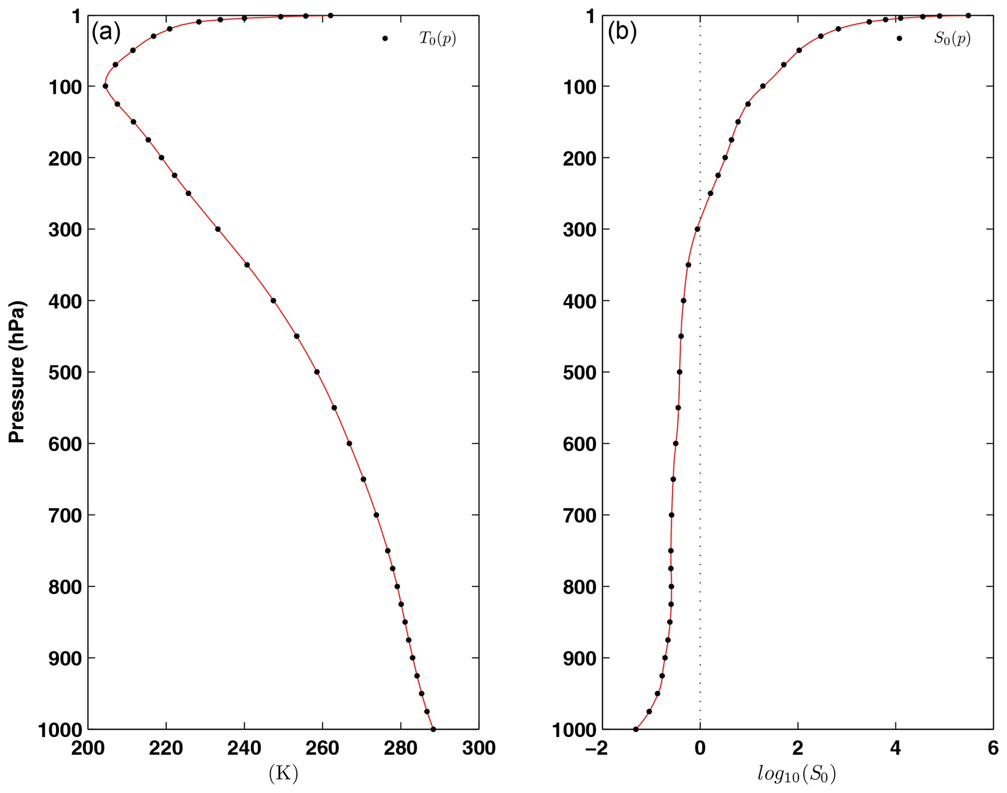
Figure 1(a) Vertical profile of temperature at the ERA-Interim pressure levels (black dots) and interpolated to GL Gaussian levels (red line). (b) Stability parameter S0 calculated from T0 at original pressure levels (black dots) and from interpolated T0 at Gaussian levels (red line). The stability parameter S0 was made dimensionless by multiplying Eq. (6) by with km. The profiles were computed from the 3-D temperature field of the ERA-Interim reanalysis, covering the period from 1 January 1979 to 31 December 2010.
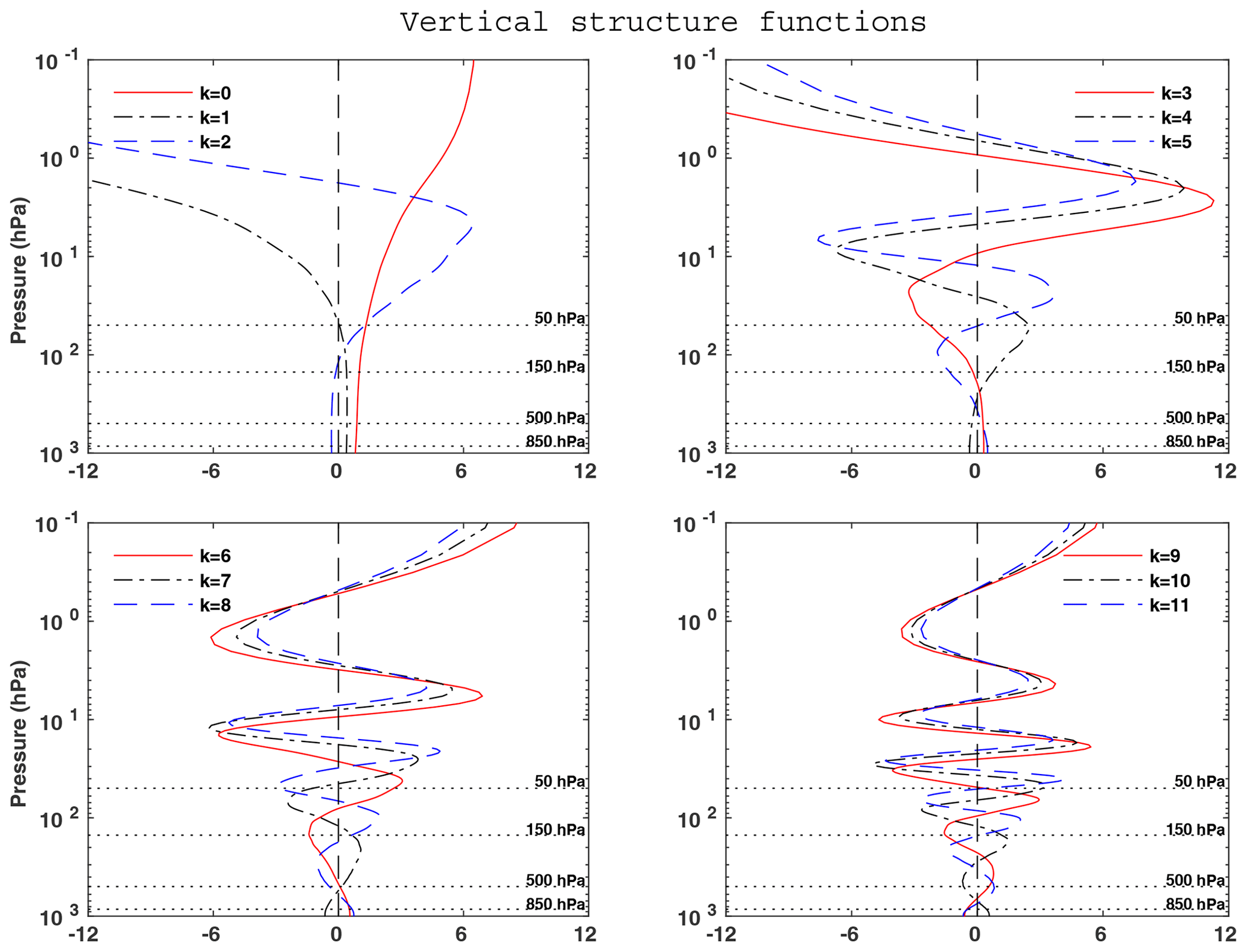
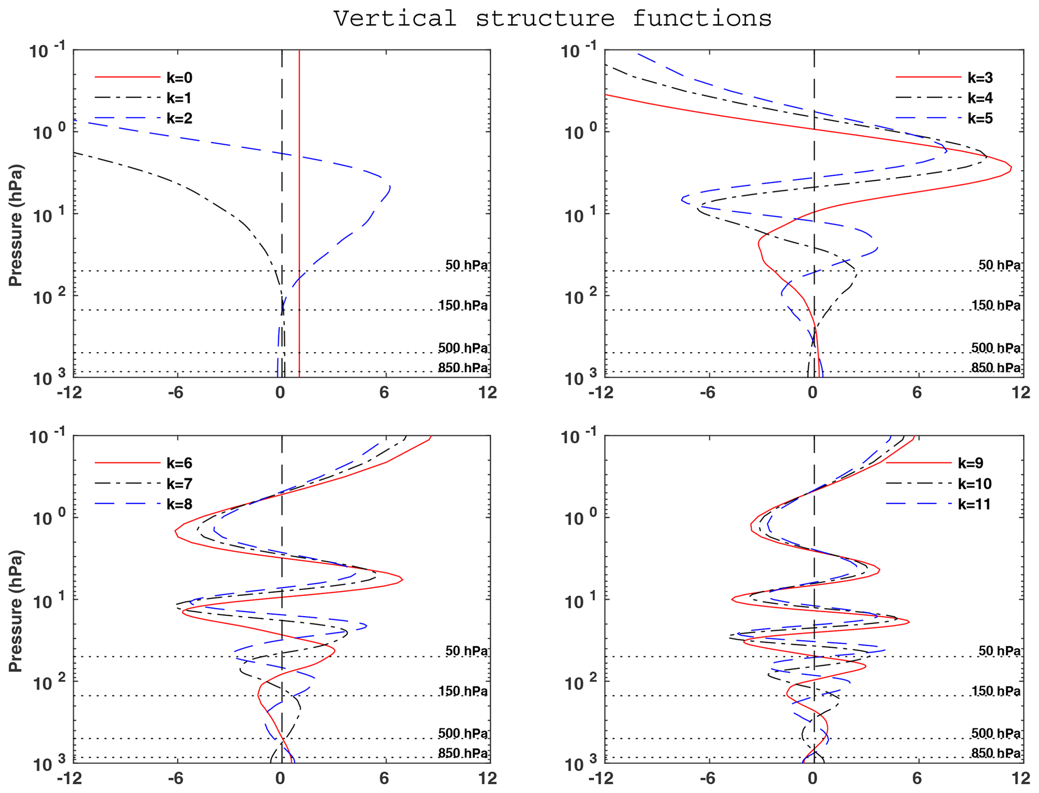
The baroclinic structures in both Figs. 2 and 3, i.e. the vertical structures with one or several nodes, are close to each other. In Fig. 3 the vertical structure function, Ψ0, is a pure barotropic vertical structure, i.e. it is a constant, and the projection of an atmospheric variable onto the barotropic mode corresponds exactly to the mass-weighted vertical mean of that variable. The vertical structure function Ψ0 in Fig. 2 is not strictly constant. Nevertheless, since Ψ0 of Fig. 2 does not change sign as its counterpart in Fig. 3 and is approximately constant in the troposphere, it is also called as barotropic mode.
2.3 Computation of the horizontal structure functions
Applying the vertical transform (18) to the system of Eqs. (8)–(10), a dimensionless equation is obtained in the following vector form (Tanaka, 1985; Marques and Castanheira, 2012):
where
The time was made dimensionless by multiplying with 2 Ω, and the vectors are made dimensionless by multiplying by the inverse of the scaling matrix Xk, which is given by
The dimensionless parameter, αk, in the linear differential matrix operator L is defined as
Equation (21) is a dimensionless form of the linearised shallow water equations.
Since Eq. (21) is a linear system with respect to λ and , the solution Wk can be expressed as zonal waves (Swarztrauber and Kasahara, 1985)
where σnlk is the dimensionless frequencies for the free waves with zonal wave number n and meridional structures Θnlk(θ). The functions are known as the horizontal structure functions, and the meridional structures Θnlk are the Hough vector functions (Longuet-Higgins, 1968; Swarztrauber and Kasahara, 1985). Substituting Eq. (27) into Eq. (21) gives
and thus the horizontal structure functions are obtained as a free eigenvalue problem. Equation (28) is referred to as the horizontal structure equation (HSE).
For n>0, there are two kinds of motion (i.e. solutions) with distinct frequencies for system (21). The first kind describes high-frequency eastward- and westward-propagating gravity inertia waves, and the second kind describes low-frequency westward-propagating rotational waves of the Rossby–Haurwitz type (Longuet-Higgins, 1968; Kasahara and Puri, 1981; Swarztrauber and Kasahara, 1985; Žagar et al., 2015b).
It can be shown that for real αk all of the frequencies σ of L are real and that any modes H corresponding to distinct frequencies are orthogonal (e.g. Swarztrauber and Kasahara, 1985; Žagar et al., 2015b). For n>0, the frequencies are distinct and thus the modes are orthogonal. However, for zonal wavenumber n=0, the rotational modes are not necessarily orthogonal because their frequencies are all zero. Nevertheless, it is possible to derive an orthogonal set of rotational modes for n=0, which are also orthogonal to the modes for n>0 (Kasahara and Puri, 1981; Shigehisa, 1983; Swarztrauber and Kasahara, 1985). Therefore, all horizontal structure functions H satisfy the orthonormal condition given by
where the superscript ∗ denotes a conjugate transpose and the right-hand side is unity if and and zero otherwise.
The Hough vector function, Θnlk(θ), has three components, zonal velocity, meridional velocity, and height, and is given by
where the factor i in front of Vnlk is introduced to account for a phase shift of π∕2 (Kasahara, 1977; Swarztrauber and Kasahara, 1985). Substituting Eq. (30) into in Eq. (29), one can see that the Hough vector functions satisfy the orthonormal condition given by
Using orthonormal condition (29), a complete set of Fourier–Hough transforms may be constructed as
In order to distinguish each wave type, i.e. the westward-propagating Rossby wave and the westward- and eastward-propagating gravity inertia waves, the meridional index l is defined as a sequence of three distinct modes, lr, lw and le, respectively (e.g. Kasahara and Puri, 1981; Marques and Castanheira, 2012).
2.4 Solutions of the horizontal structure equation
As shown in Swarztrauber and Kasahara (1985), the meridional modal functions Θnlk(θ) for the eastward and westward gravity inertia modes are symmetric (antisymmetric) with respect to the Equator for the even (odd) meridional index l. For the rotational modes, the functions Θnlk(θ) are symmetric (antisymmetric) for odd (even) l. For each vertical mode k, the frequencies σnlk and the corresponding meridional modal functions Θnlk(θ) are computed for a range of zonal wavenumbers n and meridional indices l. The computational method was developed by Swarztrauber and Kasahara (1985) and consists of expanding the eigensolutions of Eq. (28) in terms of spherical vector harmonics. The modes for n=0 are determined following the approach suggested by Shigehisa (1983), as described in Swarztrauber and Kasahara (1985).
Figure 4 shows the dimensionless frequencies σ of westward-propagating gravity inertia and rotational waves (Fig. 4a) and eastward-propagating gravity inertia waves (Fig. 4b), for the case n=1. This figure corresponds to Fig. 2 in Swarztrauber and Kasahara (1985) because we have used the same values of α as they did to compute the frequencies σ. The α used here corresponds to of Swarztrauber and Kasahara (1985). The frequencies are plotted as a function of α−1 for 10 meridional indices (), 5 symmetric (continuous lines), and 5 antisymmetric (dashed lines). The logarithm scale was used on both axes and the y axis for the westward-propagating waves has been reversed. The rotational mode lr=0 is referred to as a mixed Rossby–gravity wave because it behaves like a rotational mode for large values of α but behaves like a gravity mode for small values of α. The symmetric mode le=0 is referred to as a Kelvin wave.
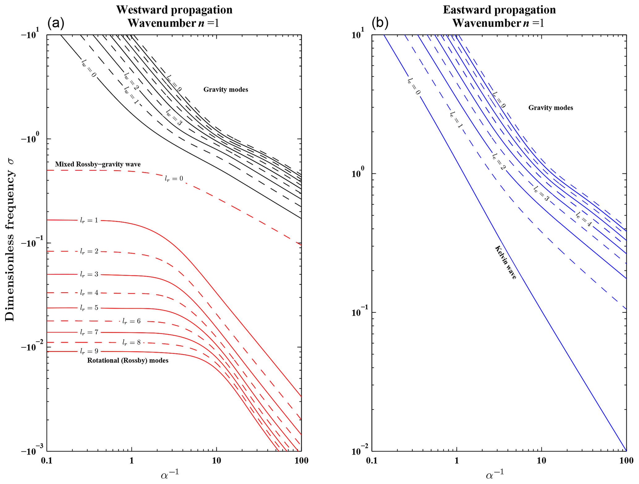
Figure 4Dimensionless frequencies σ for westward-propagating gravity waves and rotational waves (a) and for eastward-propagating gravity waves (b), plotted as a function of α−1 and for zonal wavenumber n=1.
The meaning of eastward and westward propagations is lost in the case of n=0. However, since the frequencies of gravity inertia motion appear as pairs of positive and negative values with the same magnitudes, we also use the term eastward (westward) to indicate positive (negative) frequency, as adopted by Swarztrauber and Kasahara (1985). The frequencies of the rotational motion, along with the frequencies of the gravity motion corresponding to the lowest meridional index (l=0), are zero for n=0 (Swarztrauber and Kasahara, 1985). Therefore, instead of saving zeros for all of the rotational frequencies and for the gravity frequencies corresponding to the lowest meridional index, the software computes the asymptotic rate (σa) at which those frequencies go to zero (see Eqs. 4.14 and 4.18 in Swarztrauber and Kasahara, 1985, for the definition and computational formula of σa).
Figure 5a shows the curves of asymptotic dimensionless frequencies σa in the case of n→0. The frequencies are plotted as a function of α−1 for 10 meridional indices, using a log–log scale with the y axis reversed. In this case, the lowest symmetric mode is identified as because the symmetric equations begin at index −1 (see Swarztrauber and Kasahara, 1985, for details;). The values of σa are all negative, except for the mode , which is similar to the eastward-propagating Kelvin wave in Fig. 4b. For this reason, the mode is saved as the eastward gravity mode le=0 as in Swarztrauber and Kasahara (1985). The curves for the modes behave analogously to those of rotational modes in Fig. 4a. The absolute values of dimensionless frequencies σ in the case of n=0 of the gravity waves, are illustrated in Fig. 5b for . Figure 5a and b correspond to Figs. 1 and 3 of Swarztrauber and Kasahara (1985), respectively.
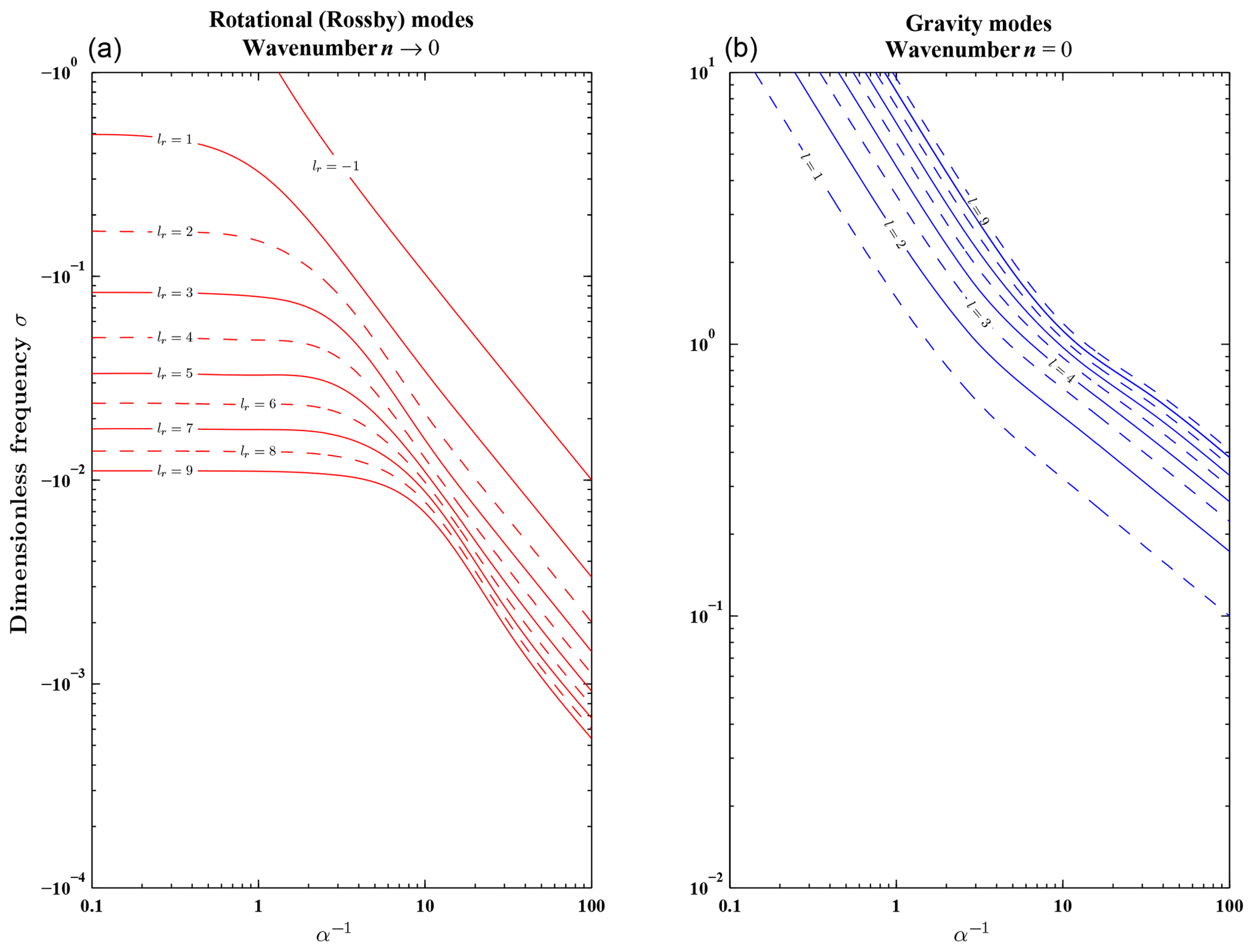
Figure 5Asymptotic dimensionless frequencies σa in the case of n→0 (a) and dimensionless frequencies for gravity waves and zonal wavenumber n=0 (b), plotted as a function of α−1.
As mentioned above, the horizontal modes include Kelvin, westward and eastward inertio-gravity (WIG and EIG, respectively), Rossby, and mixed Rossby–gravity (MRG) waves. As an illustration of the software outputs, the horizontal structure functions were calculated for each equivalent height computed in Sect. 2.2 using boundary conditions (14) and (15) (the first 12 VSFs are represented in Fig. 2), and for 43 wavenumbers () and 80 meridional modes (20 WIG, 20 EIG and 40 Rossby modes). The meridional profiles of the Hough functions corresponding to two Rossby modes lr=1 and lr=2 are shown in Fig. 6 for the barotropic mode (k=0, with h0≃9.8 km) and for two zonal wavenumbers (n=0 and n=10). Figure 7 shows the meridional profiles corresponding to the Kelvin mode (le=0) and to the Rossby mode (lr=1) for two baroclinic modes (k=1, with h1≃6.1 km and k=10, with h10≃65 m) and for two zonal wavenumbers (n=0 and n=10). By increasing the vertical index k (i.e. reducing the equivalent height hk) or the zonal wavenumber n for the same vertical index k, the horizontal structure functions become more confined around the Equator (Longuet-Higgins, 1968; Cohn and Dee, 1989; Žagar et al., 2015b).
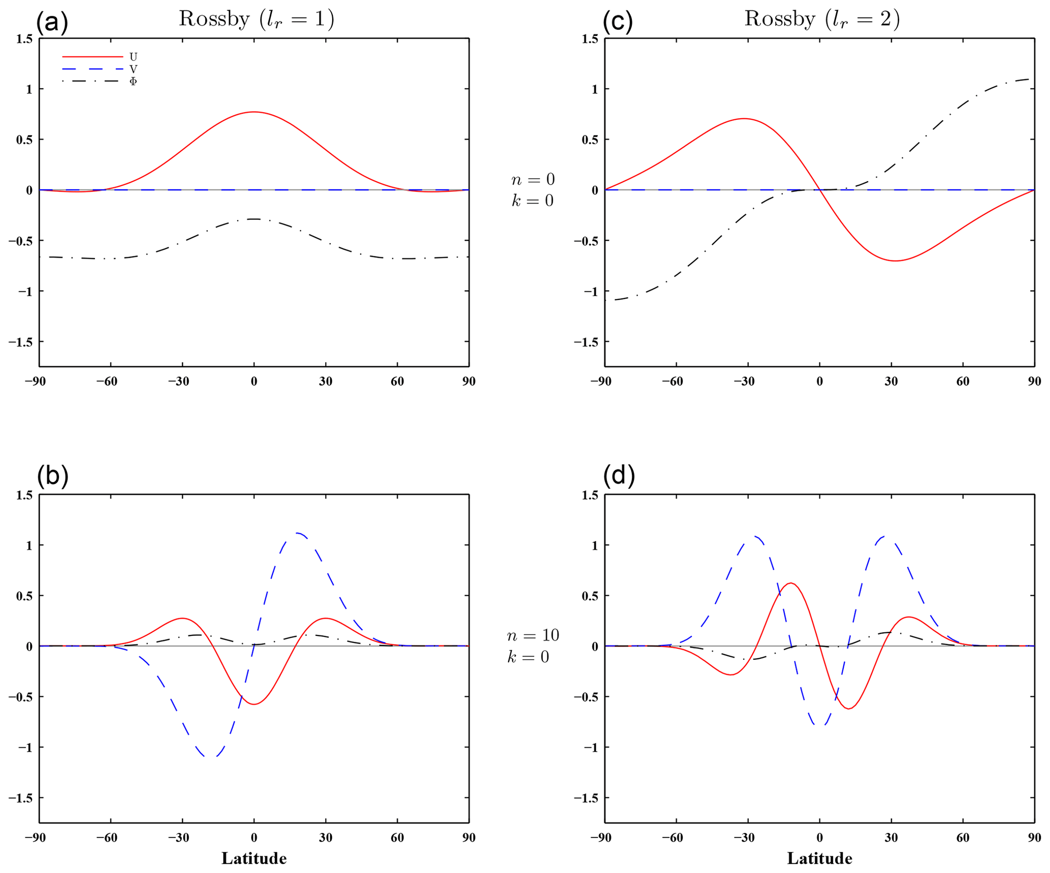
Figure 6Meridional structures of the barotropic (k=0, h0≃9.8 km) Hough harmonics for two Rossby modes, lr=1 (a, b) and lr=2 (c, d), and two zonal wavenumbers, n=0 (a, c) and n=10 (b, d). The equivalent height h0 was obtained by solving the vertical structure equation with boundary conditions (14) and (15).
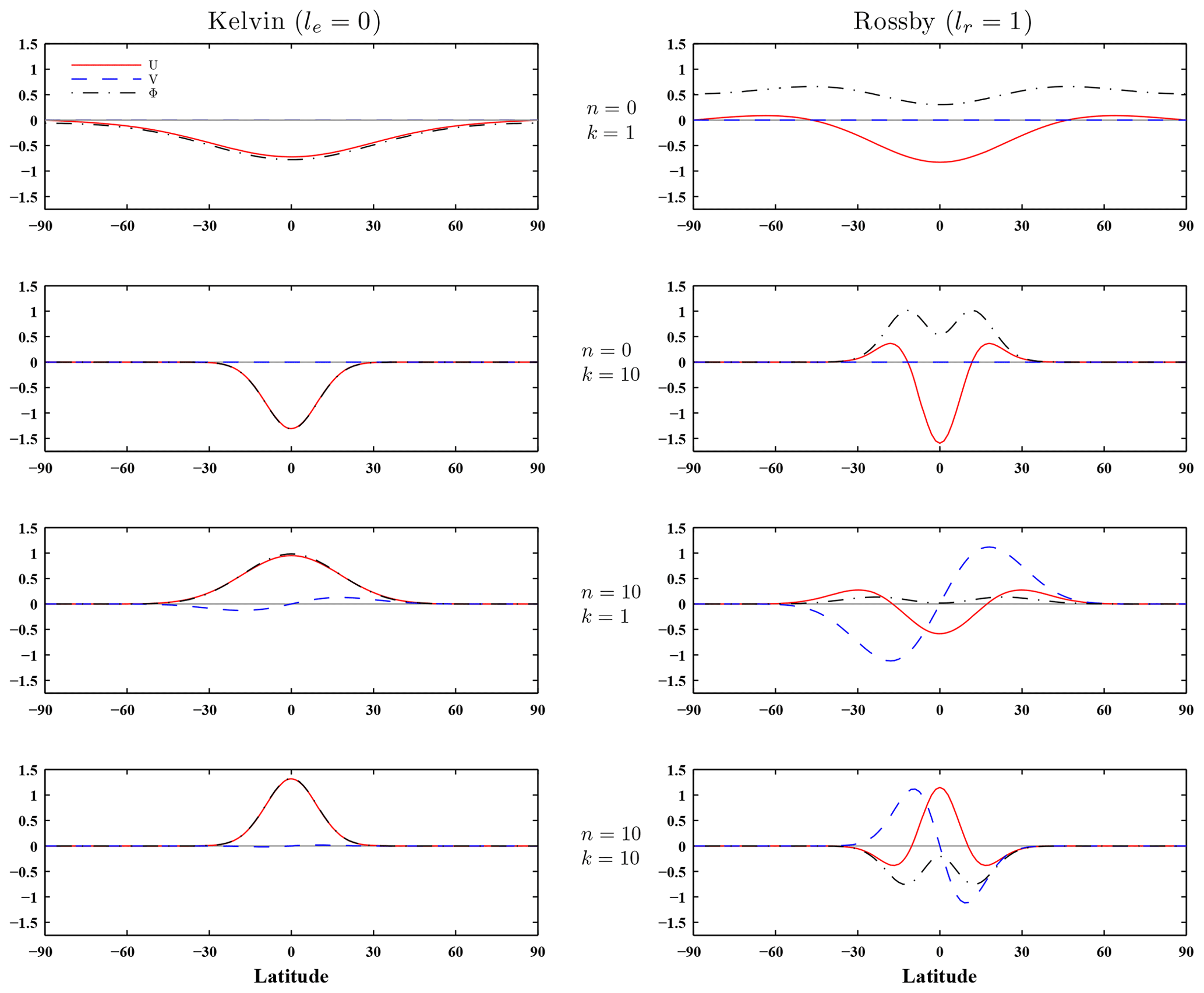
Figure 7Meridional structures of two baroclinic Hough harmonics (k=1, h1≃6.1 km and k=10, h10≃65 m) for the Kelvin mode le=0 (left column), the Rossby mode, lr=1 (right column), and for two zonal wavenumbers, n=0 and n=10. The equivalent heights hk were obtained by solving the vertical structure equation with boundary conditions (14) and (15).
2.4.1 The Haurwitz waves
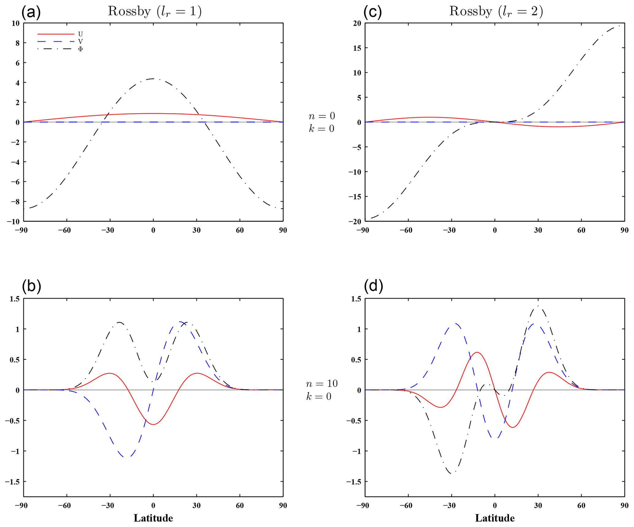
The Hough vector functions define modes in the transformed variables as given by Eq. (23). If the equivalent height hk is infinite, then transform (23) is no longer applicable. This is the case for the barotropic mode when the lower boundary condition (16) is used. However, an infinite equivalent height means that the separation constant in Eq. (12) is null, and the horizontal motion is non-divergent, and there must be no vertical dependence in the linear system (8)–(10). Consistently, the respective vertical structure is a constant. In this case, the horizontal modes are computed in the untransformed variables u,v, and ϕ as in Swarztrauber and Kasahara (1985), and are called the Rossby–Haurwitz waves. Additionally, because the linear system (8)–(10) is non-divergent, there are no WIG and EIG modes (and also no MRG mode for the zonal mean component n=0). Figure 8 shows the same meridional profiles as in Fig. 6 but for the Haurwitz modes.
2.5 3-D normal mode functions
The three-dimensional (3-D) normal mode functions (NMFs) are obtained by the product of the vertical normal modes Ψk(p) (the eigensolutions of the VSE) and the horizontal normal modes Hnlk(λ,θ) – the eigensolutions of the HSE (e.g. Kasahara, 1976; Kasahara and Puri, 1981). The 3-D NMFs, denoted by , form a complete orthogonal basis, therefore allowing us to expand the horizontal wind and the geopotential fields of the global atmosphere (Kasahara and Puri, 1981; Tanaka, 1985; Daley, 1991):
where
The expansion coefficients wnlk are obtained by means of the vertical projection onto the vertical structure functions, followed by the horizontal projection onto the horizontal structure functions:
with .
2.6 3-D normal mode energetics scheme
Using the 3-D NMFs of the linearised primitive Eqs. (8)–(10) as a basis to expand the global circulation field, Tanaka (1985) (see also Tanaka and Kung, 1988) developed a 3-D normal mode energetics (NME) scheme, which combines three one-dimensional spectral energetics in domains of the zonal wavenumber, n; meridional mode number, l; and vertical mode number, k. The 3-D NME scheme therefore complements the standard energetics in the zonal wavenumber domain of Saltzman (1957), since it can diagnose the 3-D spectral distribution of energy and energy interactions, the energetics characteristics of Rossby waves and gravity inertia waves, and the energy interaction between the barotropic and baroclinic modes (Tanaka and Kung, 1988).
Derivation of the 3-D NME may be summarised as follows.
Applying the vertical transform (18) to Eqs. (1), (2), and (7), a dimensionless equation is obtained in the following vector form:
where subscript k denotes the kth component of the vertical transform and , Wk, and L are given by Eqs. (22), (23), and (24), respectively. The dimensionless non-linear term vectors for the wind and mass fields, Ik and Jk, and the energy source or sink term due to diabatic heating and dissipation, Sk, are given by
These vectors are made dimensionless using the inverse of scaling matrix Yk, which is given by
Applying the Fourier–Hough transform (33) to (37), yields
where the complex variables wnlk, ınlk, jnlk, and snlk are the Fourier–Hough transforms of the vector variables Wk, Ik, Jk, and Sk, respectively.
The kinetic energy, K, and available potential energy, A, are defined, respectively, by
and the total energy, , is a conserved quantity of the full non-linear Eqs. (1), (2), and (7) under frictionless and adiabatic conditions (see Tanaka and Kung, 1988).
In the transformed 3-D normal mode space, the total energy Enlk associated with each mode (nlk) is
where ϵn=2 for the zonal (n=0) modes, and ϵn=1 for the eddy (n>0) modes.
Substituting Eq. (42) into the time derivatives of Eq. (45), the energy balance equations for the 3-D normal modes are finally obtained as
where
The terms Inlk,Jnlk, and Snlk that contribute to the time change of Enlk are, respectively, associated with non-linear interactions of kinetic and available potential energies and with an energy source or sink due to diabatic heating and dissipation. The spectra of these terms can therefore be analysed separately for the zonal mean and eddy components, the barotropic and baroclinic modes, and the Rossby and gravity waves (Tanaka and Kung, 1988).
As another illustration of the capabilities of the current software, in Fig. 9 the spectra for total energy E (Fig. 9a, b, c), interactions of available potential energy J (Fig. 9d, e, f), and interactions of kinetic energy I are shown (Fig. 9g, h, i). Figure 9a, d, and g contain the wavenumber spectra, whereas Fig. 9b, e, and h and Fig. 9c, f, and i show the vertical spectra for the zonal mean and eddy components, respectively. In each panel the total spectra are represented, along with the contributions of the Rossby and gravity components. These spectra were computed using 34 years of ERA-Interim reanalysis (Dee et al., 2011) data covering the period from 1 January 1979 to 31 December 2012. The horizontal wind (u,v), pressure velocity (ω), temperature, and geopotential fields were obtained with grid resolution for the 37 isobaric levels from 1000 to 1 hPa at time intervals of 6 h. The solutions of the VSE (13), with boundary conditions (16) and (15), were approximated using 57 Legendre polynomials and 37 vertical modes were retained. The zonal wavenumber has been truncated at n=42. The spectra were computed at each time step (6-hourly) and then averaged over the 30-year period.
A detailed analysis of the spectra in Fig. 9 is beyond the scope of this study, but some of its characteristics are mentioned. The wavenumber energy spectrum of Rossby modes approximately follows the −3 power law over the synoptic and mesoscale region, while that of the gravity modes has approximately a slope, which is in line with the literature (e.g. Charney, 1971; Nastrom and Gage, 1985; Tanaka, 1985; Tanaka et al., 1986; Terasaki and Tanaka, 2007). The zonal mean available potential energy is transferred into eddy available potential energy essentially due to the Rossby waves, with a small contribution by planetary-scale gravity waves, as indicated by the positive values in the wavenumber spectra of J. On the other hand, the wavenumber spectra of I indicate that the Rossby waves transfer energy out of the eddy kinetic energy reservoir, whereas the smaller quantity of energy transferred by the gravity waves is in the opposite direction. The vertical spectra for I shows that the eddy kinetic energy contained in the Rossby baroclinic modes is transferred into the Rossby barotropic modes of both zonal mean and eddy components, and also into baroclinic zonal mean kinetic energy. Again, it is seen that the transfer of kinetic energy due to the gravity waves is in the opposite direction.
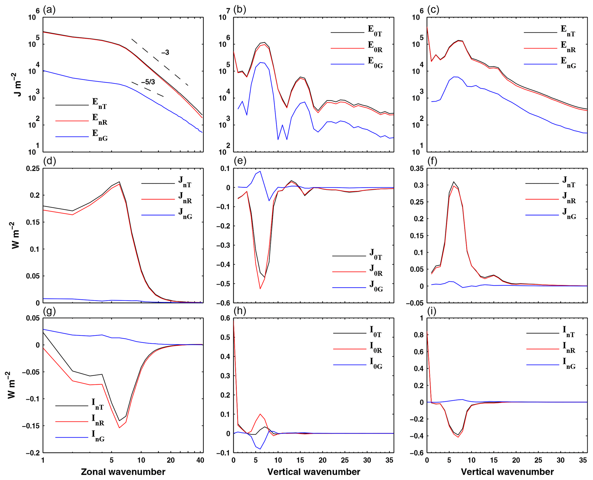
Figure 9Spectra of total energy E (a, b, c) and of non-linear interactions of available potential J (d, e, f) and kinetic I (g, h, i) energies, in the zonal wavenumber (a, d, g) and the vertical index, separately, for the zonal (b, e, h) (0) and eddy (c, f, i) (n) components. In each panel the contributions of the Rossby (R) and gravity (G) components to the total (T) spectra of energy or energy interactions are represented.
A disadvantage of the 3-D NME is that one cannot separate the available potential and kinetic energies, only the total energy (Enlk) associated with each mode can be calculated. Consequently, the conversion rate of available potential energy into kinetic energy also cannot be accessed. However, the separation of the available potential and kinetic energies can be performed if one uses only the expansions in the vertical and wavenumber domains. This reasoning led Marques and Castanheira (2012) to present a normal mode energetics formulation that performs an explicit evaluation of the available potential and kinetic energies, as well as the conversion rates between them. In addition, the generation and dissipation rates and the non-linear interactions of each energy form can be performed in both the zonal wavenumber and vertical mode domains. Using the vertical normal mode basis that results from applying lower boundary condition (14) and (15), and then performing the vertical and the zonal wavenumber (Fourier) expansions, the set of balance equations for the kinetic energy (K) and available potential energy (A) is given by (see Marques and Castanheira, 2012, for details)
where
and

Figure 10Extended energy cycle diagram describing the flow of energy among the zonal mean and eddy components and among the barotropic and baroclinic components for ERA-Interim in DJF (top values) and JJA (bottom values) climates. Units are 105 J m−2 for energy levels and W m−2 for conversion and transfer rates and generation and dissipation rates.
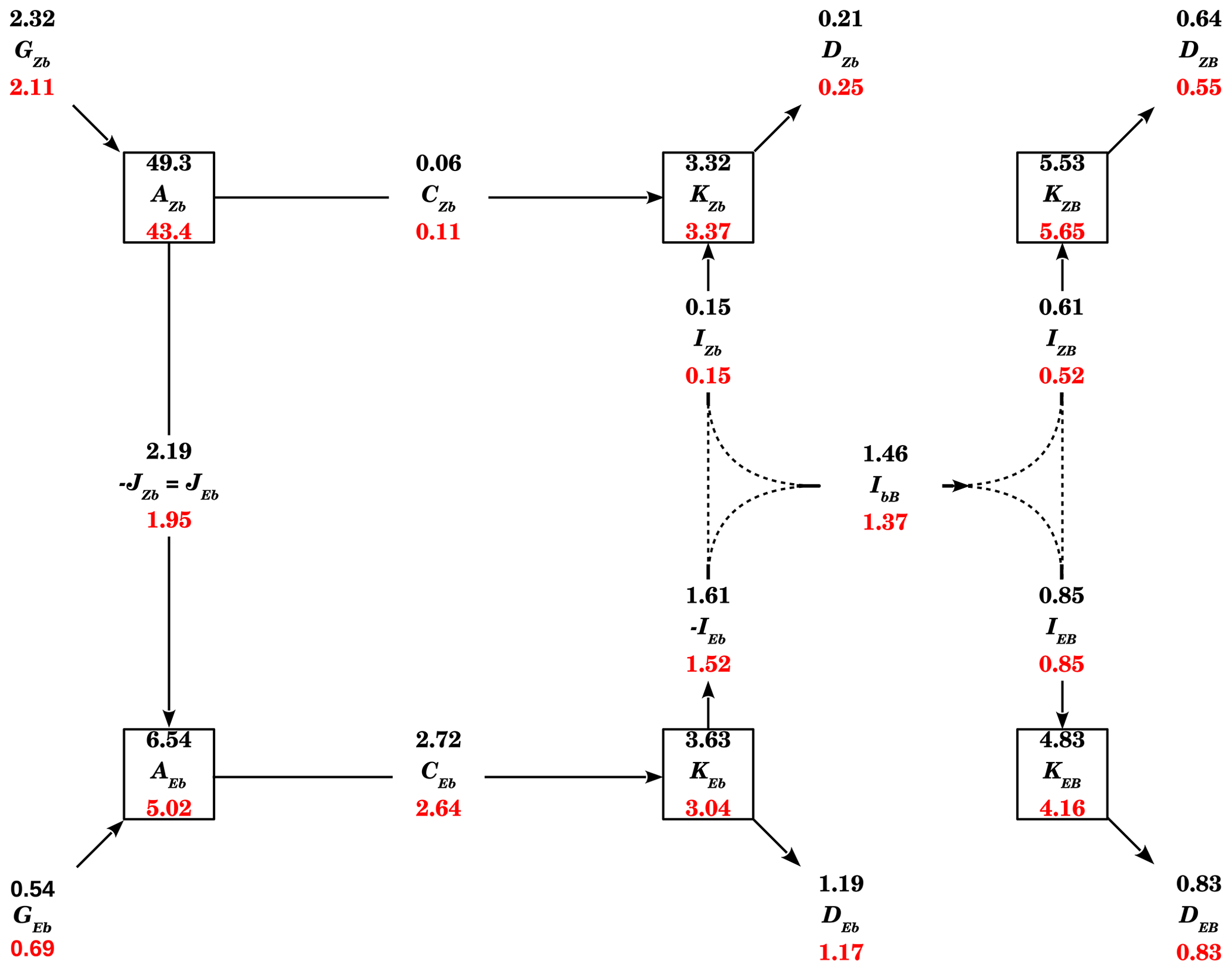
The term Cnk represents the conversion of available potential energy into kinetic energy, whereas Ink (Jnk) represents interactions or exchanges of kinetic (available potential) energy between different scales or types of motion. Finally, the dissipation of kinetic energy and the generation of available potential energy, due to diabatic processes, are represented by terms Dnk and Gnk, respectively, and may be computed as residuals from balance Eqs. (50) and (51). The calculated energetic terms may then be used to construct an extended energy cycle diagram, as in Fig. 7 of Marques and Castanheira (2012) (see also Fig. 6 in Marques et al., 2014). Such an extended energy cycle diagram is illustrated in Fig. 10, in which the boxes represent the levels of energy and the arrows the energy generation and dissipation rates and the energy conversion and transfer rates. The estimates in the diagram were based on the same 34 years of ERA-Interim reanalysis mentioned above for the 3-D spectra of E, J, and I. The solutions of the VSE (13) were obtained using boundary conditions (14) and (15). The energetic terms were computed at each time step (6-hourly) and then averaged over the 34-year period to obtain the corresponding mean values for the northern winter (DJF) and summer (JJA) seasons, which are represented as the top (black) and bottom (red) values in Fig. 10.
The energy cycle diagram of Fig. 10 describes the flow of energy among the zonal mean and eddy components, and also among the barotropic and baroclinic components. All terms in the diagram are decomposed into the zonal mean (n=0) and eddy (n≥1) components, which are denoted, respectively, by subscripts Z and E. Each one of these components is also decomposed into the barotropic (k=0) and baroclinic (k≥1) components by using the extra subscripts B and b, respectively. The two exceptions are the barotropic–baroclinic interactions of available potential energy, denoted by JBb, and the baroclinic–barotropic interactions of kinetic energy, which is represented as IbB. These values represent the balances of the flows of kinetic energy and available potential energy between the barotropic and baroclinic components and both zonal mean and eddies, implying that the energy flows represented by the dotted lines in the diagram cannot by quantified individually. These flows are associated with eddy generation by barotropic instability and the barotropic decay of baroclinic eddies (see Marques and Castanheira, 2012, and references therein, for details).
As an alternative, Marques and Castanheira (2017) and Castanheira and Marques (2019) presented a similar NME scheme, but using the vertical normal mode basis that results from applying lower boundary condition (16) in place of (14). The main difference between the NME schemes presented in Marques and Castanheira (2012) and in Marques and Castanheira (2017) is that in the latter, the first vertical structure is strictly constant, which implies that its vertical derivative is null and there is no available potential energy associated with the barotropic mode (k=0). Therefore, the terms An0, Cn0, Jn0, and Gn0 are null in this variant of the energetics scheme. All baroclinic terms (k≥1) have identical expressions in both NME schemes. The terms associated with the kinetic energy of the barotropic component are calculated formally with identical expressions in both NME schemes. However, a constant h0 cannot be derived from the eigenvalues of the VSE (13). In this case the smallest eigenvalue is null and corresponds to the separation constant in Eq. (12) being null. For such a case, it is not possible to define an equivalent height as it was in Eq. (12). In order to keep the expressions for the barotropic and baroclinic terms formally identical in both NME schemes, the software fixes h0=1m, when the boundary condition (16) is used. Calculating the terms given by Eqs. (52)–(58) in this way, (50) and (51) may also be used to construct an extended energy cycle diagram as illustrated in Fig. 11 (see also Fig. A2 in Marques and Castanheira, 2017). In this case, there is no barotropic branch in the available potential energy side, as compared to extended energy cycle diagram of Fig. 10. The estimates in this diagram were based on the same data as those of Fig. 10. The solutions of the VSE were also approximated using 57 Legendre polynomials, retaining 37 vertical modes. The same zonal wavenumbers as those for the estimates in Fig. 10 were also considered.
Although boundary condition (16) may be seen as somewhat unrealistic, it presents some useful features. First, using the boundary conditions (15) and (16), it can easily be shown that the total energy is exactly conserved by full non-linear Eqs. (1)–(5), in the case of frictionless adiabatic motions (see Tanaka and Kung, 1988). Moreover, an extra surface term, which was interpreted by Tanaka and Kung (1988) as a geopotential flux across the lower boundary, does not appear in the available potential energy as defined by Eq. (44), when the boundary condition (16) is used. Another feature of (16) is that the barotropic mode represents the mass-weighted average of the circulation field.
The use of the boundary condition (14) may seem more realistic, but in order to guarantee the conservation of energy for frictionless adiabatic motions it is necessary to impose a non-slipping condition at p=ps, though this may seem contradictory with the absence of friction.
The software presented here consists of tools or functions for specific tasks and includes a Python and a MATLAB version. The Python version requires NumPy and SciPy modules and works with both Python 2 and 3. The netCDF4 library is recommended. The input–output data format for each function may be either the native format of the chosen version, i.e. “.mat” for MATLAB and “.npz” for Python, or netCDF for both versions.
The tasks to be achieved with the functions in the software include the solution of the VSE (13), the solution of HSE (28), and the computation of complex expansion coefficients wnlk, ınlk, and jnlk, which are the vertical Fourier–Hough transforms of the dependent variable vector , of the non-linear term vector due to wind field, and of the non-linear term due to mass field, respectively. In addition, the software also permits the computation of vertical transforms of the terms in the normal mode energetics formulation presented by Marques and Castanheira (2012) or its alternative presented by Marques and Castanheira (2017) and Castanheira and Marques (2019). These terms constitute the set of balance Eqs. (50) and (51), and its expressions are given in Eqs. (52)–(64). With these vertical transforms the user may compute the global energy cycle in the wavenumber and vertical domains (as in Marques and Castanheira, 2012, 2017; Castanheira and Marques, 2019), with the dissipation and generation terms computed as residuals from Eqs. (50) and (51).
Other applications of this software include the spatial-scale filtering of atmospheric motion and filtering of balanced motion and mass unbalanced motions by retaining an appropriate subset of terms in the expansion (34) (e.g. Castanheira and Marques, 2015; Žagar et al., 2020). Furthermore, the solutions of HSE, i.e. the Hough vector functions (Θnlk(θ)), can be used as meridional basis functions onto which dynamical data may be projected. This can be an alternative tool for investigating studies on tropical convection as in Yang et al. (2003) and Gehne and Kleeman (2012), which have used parabolic cylinder functions as meridional basis functions. All of these features are useful both in data analysis and in assessment of general circulation atmospheric models (e.g. Žagar et al., 2020).
-
Vertical structure.
The vertical structure equation (VSE), (13), is solved with a function named vertical_structure that uses the spectral method introduced by Kasahara (1984). The function requires the mean vertical profile of temperature T0, defined on pressure levels, and the pressure levels as inputs, returning the vertical structure functions (Ψk(p)) and equivalent heights (hk). The VSE may be solved using either one of the two pairs of boundary conditions, as described in Sect. 2.2. These pairs of boundary conditions are controlled by the input argument ws0. When ws0=False (the default) the VSE is solved using boundary conditions (14) and (15), whereas when ws0=True the VSE is solved using boundary conditions (16) and (15). In the latter case the first vertical structure is strictly constant and the associated equivalent height is infinite.
-
Horizontal structure.
The solution of HSE (21) is obtained with a function called hough_functions. It uses the computational method developed by Swarztrauber and Kasahara (1985), which consists of expanding the eigensolutions of Eq. (28) in terms of spherical vector harmonics. The function inputs are the equivalent heights (hk) and the user-defined parameters for the maximum zonal wavenumber, the total number of Rossby modes and half the number of gravity modes used in the expansion, along with the latitude points, which may be linear (the default) or Gaussian. It returns the Hough vector functions (Θnlk(θ)) and the frequencies of the modes. In the output, the meridional modes are written in the following order: first the westward gravity modes, then the eastward gravity modes, and finally the (westward) Rossby modes. Both types of gravity modes are written following the symmetric–antisymmetric mode order, whereas the order for Rossby modes is reversed. If the VSE (13) is solved using boundary conditions (16) and (15), then the solutions for the barotropic mode returned by hough_functions are the Haurwitz waves (Swarztrauber and Kasahara, 1985). This is controlled internally by hough_functions which calls functions named hvf_baroclinic and hvf_barotropic for the Haurwitz modes.
-
Expansion coefficients.
The complex expansion coefficients wnlk, ınlk, and jnlk may be obtained with a function called expansion_coeffs. The inputs are the vertical structure functions (Ψk(p)), the equivalent heights (hk), the Hough vector functions (Θnlk(θ)), and a data structure with appropriate fields. For the expansion coefficients wnlk a data structure with fields is required (recall that field ϕ corresponds to the deviations from a hydrostatic reference state ϕ0(p)). The computation of expansion coefficients ınlk and jnlk requires data structures with fields [I1,I2] and [J3], respectively. Each one of these fields need to be pre-computed by the user and correspond to the terms between square brackets of Eqs. (59), (60) and (61), respectively (note that in Eq. 61 the vertical derivative is outside the square brackets, and that this is accounted for in the expansion_coeffs function). The returned coefficients, wnlk, ınlk and jnlk, may then be used to compute the 3-D spectrum of total energy (Enlk) and of the non-linear interactions of kinetic (Inlk) and available potential (Jnlk) energies (see Fig. 9), using Eqs. (45), (47), and (48), respectively.
-
The inverse transforms.
The zonal and meridional wind, u and v, and geopotential perturbation ϕ (from the reference geopotential), as given by Eq. (34), can be obtained with the function inv_expansion_coeffs. By choosing an appropriate subset of modes, this function can be used for spatial-scale filtering of atmospheric motion, balanced and mass unbalanced motions, and barotropic and baroclinic components. Moreover, choosing the appropriate meridional indices the filtering can be used to isolate tropical components of the atmospheric circulation. The function requires the vertical structure functions (Ψk(p)); the equivalent heights (hk); the Hough vector functions (Θnlk(θ)); the complex expansion coefficients (wnlk); the pressure levels (in hPa); the longitudes (in degrees); and the wavenumber, meridional, and vertical indices as inputs. In addition, the user can choose to compute all three fields, u,v and ϕ (the default), or only a subset of those, which is controlled by the input argument uvz.
-
Vertical and Hough transforms.
All functions described above have the same name in both versions, MATLAB and Python, differing only in the file extension (“.m” and “.py”, respectively). The software tools presented here include two more functions used to compute the vertical and the Hough transforms. In the MATLAB version there are two separate functions, vertical_transform.m and hough_transform.m, whereas for Python both are included in module transforms.py, being invoked as transforms.vertical and transforms.hough. The vertical and Hough transforms are used by the expansion_coeffs function, but they may be also executed independently by the user. For example, the vertical_transform function (or transforms.vertical) may be used to compute the vertical transforms of u, v, ϕ, I1, I2, and J3. Again, I1, I2, and J3 correspond to the terms between square brackets of Eqs. (59), (60), and (61). The computation of these six vertical transforms constitute the essential task to obtain the global energy cycle in the wavenumber and vertical domains as in Marques and Castanheira (2012) or Marques and Castanheira (2017) (see also Castanheira and Marques, 2019). Having these vertical transforms, all of the terms of the normal mode energetics formulation, represented by balance Eqs. (50) and (51), may then be easily obtained using Eqs. (52)–(56), with the remainder dissipation and generation terms computed as residuals from Eqs. (50) and (51).
The exact version of the software code used to produce the results presented in this paper is archived on Zenodo (https://doi.org/10.5281/zenodo.3631310, Marques et al., 2020). A step-by-step tutorial is included in the repository for both Python and MATLAB. Also included are the mean vertical profiles of temperature and geopotential, computed from 32 years (1979–2010) of the ERA-Interim reanalysis data as described in the text (see Sect. 2.2). These two vertical profiles, along with the horizontal wind (u, v), pressure velocity (ω), temperature, and geopotential fields that may be obtained from the ERA-Interim data server with grid resolution for all of the provided 37 isobaric levels from 1000 to 1 hPa, at time intervals of 6 h, are the only datasets needed to obtain all of the figures in the paper. The two exceptions are Figs. 4 and 5, for which we have used the same values as Swarztrauber and Kasahara (1985); see, for example, their Table 5. Note that our α corresponds to their .
CAFM conceived the idea, wrote the initial version of the software code for MATLAB, and tested the final version of the software for both MATLAB and Python. MMA wrote the software code for Python and the final version of the code for MATLAB and collaborated in the tests of the software. JMC elaborated the structure of the software and collaborated in writing the initial version of the software code for MATLAB and in the software tests. All authors contributed to writing the manuscript.
The authors declare that they have no conflict of interest.
The code is made publicly available without any warranty.
Carlos A. F. Marques was supported by the Portuguese Foundation for Science and Technology (FCT) under grant no. SFRH/BPD/76232/2011. The ERA-Interim data have been obtained from the ECMWF data server. Thanks are due to FCT/MCTES for the financial support to CESAM (UIDP/50017/2020+UIDB/50017/2020) through national funds.
This research has been supported by the Portuguese Foundation for Science and Technology (FCT) (grant no. SFRH/BPD/76232/2011) and by FCT/MCTES through national funds for the financial support to CESAM (UIDP/50017/2020+UIDB/50017/2020).
This paper was edited by David Ham and reviewed by two anonymous referees.
Blaauw, M. and Žagar, N.: Multivariate analysis of Kelvin wave seasonal variability in ECMWF L91 analyses, Atmos. Chem. Phys., 18, 8313–8330, https://doi.org/10.5194/acp-18-8313-2018, 2018. a
Castanheira, J. M. and Marques, C. A. F.: Convectively Coupled Equatorial Waves Diagnosis using 3–D Normal Modes, Q. J. Roy. Meteor. Soc., 141, 2776–2792, https://doi.org/10.1002/qj.2563, 2015. a, b, c
Castanheira, J. M. and Marques, C. A. F.: The energy cascade associated with daily variability of the North Atlantic Oscillation, Q. J. Roy. Meteor. Soc., 145, 197–210, https://doi.org/10.1002/qj.3422, 2019. a, b, c, d, e, f
Castanheira, J. M., DaCamara, C. C., and Rocha, A.: Numerical solutions of the vertical structure equation and associated energetics, Tellus, 51A, 337–348, 1999. a, b
Castanheira, J. M., Graf, H.-F., DaCamara, C. C., and Rocha, A.: Using a Physical Reference Frame to Study Global Circulation Variability, J. Atmos. Sci., 59, 1490–1501, https://doi.org/10.1175/1520-0469(2002)059<1490:UAPRFT>2.0.CO;2, 2002. a
Charney, J. G.: Geostrophic turbulence, J. Atmos. Sci., 28, 1087–1095, 1971. a
Cohn, S. E. and Dee, D. P.: An analysis of the vertical structure equation for arbitrary thermal profiles, Q. J. Roy. Meteor. Soc., 115, 143–171, 1989. a, b, c
Daley, R.: Atmospheric data analysis, Cambridge University Press, Cambridge, UK, 1991. a, b, c
Dee, D. P., Uppala, S. M., Simmons, A. J., Berrisford, P., Poli, P., Kobayashi, S., Andrae, U., Balmaseda, M. A., Balsamo, G., Bauer, P., Bechtold, P., Beljaars, A. C. M., van de Berg, L., Bidlot, J., Bormann, N., Delsol, C., Dragani, R., Fuentes, M., Geer, A. J., Haimberger, L., Healy, S. B., Hersbach, H., Hólm, E. V., Isaksen, L., Kållberg, P., Köhler, M., Matricardi, M., McNally, A. P., Monge-Sanz, B. M., Morcrette, J.-J., Park, B.-K., Peubey, C., de Rosnay, P., Tavolato, C., Thépaut, J.-N., and Vitart, F.: The ERA–Interim reanalysis: configuration and performance of the data assimilation system, Q. J. Roy. Meteor. Soc., 137, 553–597, https://doi.org/10.1002/qj.828, 2011. a, b
Franzke, C. L. E., Jelic, D., Lee, S., and Feldstein, S. B.: Systematic decomposition of the MJO and its Northern Hemispheric extratropical response into Rossby and inertio-gravity components, Q. J. Roy. Meteor. Soc., 145, 1147–1164, https://doi.org/10.1002/qj.3484, 2019. a
Gehne, M. and Kleeman, R.: Spectral Analysis of Tropical Atmospheric Dynamical Variables Using a Linear Shallow-Water Modal Decomposition, J. Atmos. Sci., 69, 2300–2316, 2012. a
Kasahara, A.: Normal modes of ultralong waves in the atmosphere, Mon. Weather Rev., 104, 669–690, 1976. a
Kasahara, A.: Numerical Integration of the Global Barotropic Primitive Equations with Hough Harmonic Expansions, J. Atmos. Sci., 34, 687–701, 1977. a
Kasahara, A.: The Linear Response of a Stratified Global Atmosphere to Tropical Thermal Forcing, J. Atmos. Sci., 41, 2217–2237, 1984. a, b
Kasahara, A. and Puri, K.: Spectral representation of three-dimensional global data by expansion in normal mode functions, Mon. Weather Rev., 109, 37–51, 1981. a, b, c, d, e, f, g, h
Kitsios, V., O'Kane, T. J., and Žagar, N.: A Reduced-Order Representation of the Madde–Julian Oscillation Based on Reanalyzed Normal Mode Coherences, J. Atmos. Sci., 76, 2463–2480, https://doi.org/10.1175/JAS-D-18-0197.1, 2019. a
Longuet-Higgins, M. S.: The eigenfunctions of Laplace's tidal equations over a sphere, Philos. T. Roy. Soc. London, A262, 511–607, 1968. a, b, c
Marques, C. A. F. and Castanheira, J. M.: A detailed normal mode energetics of the general circulation of the atmosphere, J. Atmos. Sci., 69, 2718–2732, 2012. a, b, c, d, e, f, g, h, i, j, k, l, m
Marques, C. A. F. and Castanheira, J. M.: Barotropic decelerations of the southern stratospheric polar vortex, Q. J. Roy. Meteor. Soc., 143, 744–755, https://doi.org/10.1002/qj.2961, 2017. a, b, c, d, e, f
Marques, C. A. F. and Castanheira, J. M.: Diagnosis of Free and Convectively Coupled Equatorial Waves, Math. Geosci., 50, 585–606, https://doi.org/10.1007/s11004-018-9729-y, 2018. a, b
Marques, C. A. F., Castanheira, J. M., and Rocha, A.: Changes in the normal mode energetics of the general atmospheric circulation in a warmer climate, Clim. Dynam., 42, 1887–1903, https://doi.org/10.1007/s00382-013-1750-8, 2014. a, b
Marques, C. A. F., Marta-Almeida, M., and Castanheira, J. M.: NMF3D – tridimensional normal mode functions, Zenodo, https://doi.org/10.5281/zenodo.3631310, 2020. a
Nastrom, G. D. and Gage, K. S.: A climatology of atmospheric wavenumber spectra of wind and temperature observed by commercial aircraft, J. Atmos. Sci., 42, 950–960, 1985. a
Saltzman, B.: Equations governing the energetics of the larger scales of atmospheric turbulence in the domain of wave number, J. Meteorol., 14, 513–523, 1957. a
Shigehisa, Y.: Normal modes of the shallow water equations for zonal wavenumber zero, J. Meteorol. Soc. Jpn., 61, 479–494, 1983. a, b
Swarztrauber, P. N. and Kasahara, A.: The vector harmonic analysis of Laplace's tidal equations, SIAM J. Sci. Stat. Comput., 6, 464–491, 1985. a, b, c, d, e, f, g, h, i, j, k, l, m, n, o, p, q, r, s, t, u
Tanaka, H. L.: Global energetics analysis by expansion into three-dimensional normal-mode functions during the FGGE winter, J. Meteorol. Soc. Jpn., 63, 180–200, 1985. a, b, c, d, e, f, g
Tanaka, H. L. and Kung, E. C.: Normal-mode energetics of the general circulation during the FGGE year, J. Atmos. Sci., 45, 3723–3736, 1988. a, b, c, d, e, f, g, h
Tanaka, H. L. and Seki, S.: Development of a Three-Dimensional Spectral Linear Baroclinic Model and its Application to the Baroclinic Instability Associated with Positive and Negative Arctic Oscillation Indices, J. Meteorol. Soc. Jpn. Ser. II, 91, 193–213, https://doi.org/10.2151/jmsj.2013-207, 2013. a
Tanaka, H. L. and Tokinaga, H.: Baroclinic Instability in High Latitudes Induced by Polar Vortex: A Connection to the Arctic Oscillation, J. Atmos. Sci., 59, 69–82, https://doi.org/10.1175/1520-0469(2002)059<0069:BIIHLI>2.0.CO;2, 2002. a
Tanaka, H. L., Kung, E. C., and Baker, W. E.: Energetics analysis of the observed and simulated general circulation using three-dimensional normal mode expansions, Tellus, 38A, 412–428, 1986. a
Terasaki, K. and Tanaka, H. L.: An Analysis of the 3-D Atmospheric Energy Spectra and Interactions Using Analytical Vertical Structure Functions and Two Reanalyses, J. Meteorol. Soc. Jpn., 85, 785–796, 2007. a
Yamagami, A. and Tanaka, H. L.: Analysis of Unstable Solution with an MJO Structure Using a Three-Dimensional Spectral Linear Baroclinic Model, SOLA, 10, 103–107, https://doi.org/10.2151/sola.2014-021, 2014. a
Yamagami, A. and Tanaka, H. L.: Characteristics of the JRA-55 and ERA-Interim Datasets by Using the Three-Dimensional Normal Mode Energetics, SOLA, 12, 27–31, https://doi.org/10.2151/sola.2016-006, 2016. a
Yang, G.-Y., Hoskins, B., and Slingo, J.: Convectively Coupled Equatorial Waves: A New Methodology for Identifying Wave Structures in Observational Data, J. Atmos. Sci., 60, 1637–1654, 2003. a
Žagar, N., Buizza, R., and Tribbia, J.: A Three-Dimensional Multivariate Modal Analysis of Atmospheric Predictability with Application to the ECMWF Ensemble, J. Atmos. Sci., 72, 4423–4444, https://doi.org/10.1175/JAS-D-15-0061.1, 2015a. a
Žagar, N., Kasahara, A., Terasaki, K., Tribbia, J., and Tanaka, H.: Normal-mode function representation of global 3-D data sets: open-access software for the atmospheric research community, Geosci. Model Dev., 8, 1169–1195, https://doi.org/10.5194/gmd-8-1169-2015, 2015b. a, b, c, d
Žagar, N., Kosovelj, K., Manzini, E., Martin, H., and Castanheira, J.: An assessment of scale-dependent variability and bias in global prediction models, Clim. Dynam., 54, 287–306, https://doi.org/10.1007/s00382-019-05001-x, 2020. a, b